Model AdequacyModel Adequacy
Testing Assumptions, Testing Assumptions, Checking for Outliers, and Checking for Outliers, and
MoreMore
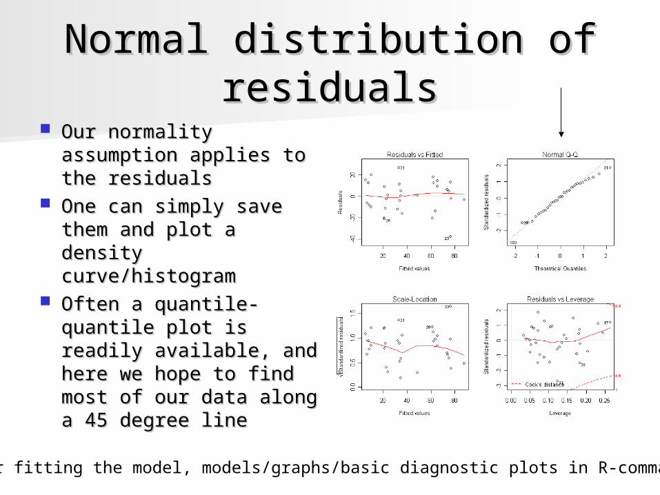
Normal distribution of Normal distribution of residualsresiduals
Our normality Our normality assumption applies to assumption applies to the residualsthe residuals
One can simply save One can simply save them and plot a density them and plot a density curve/histogramcurve/histogram
Often a quantile-Often a quantile-quantile plot is readily quantile plot is readily available, and here we available, and here we hope to find most of hope to find most of our data along a 45 our data along a 45 degree linedegree line
*After fitting the model, models/graphs/basic diagnostic plots in R-commander
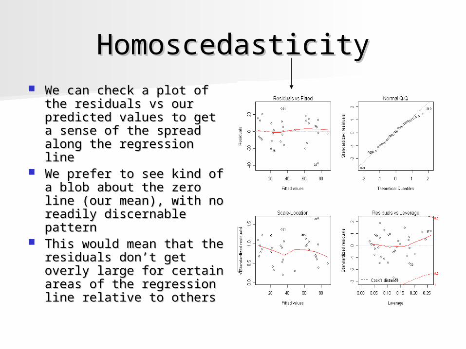
HomoscedasticityHomoscedasticity We can check a plot of the We can check a plot of the
residuals vs our predicted residuals vs our predicted values to get a sense of values to get a sense of the spread along the the spread along the regression lineregression line
We prefer to see kind of a We prefer to see kind of a blob about the zero line blob about the zero line (our mean), with no readily (our mean), with no readily discernable patterndiscernable pattern
This would mean that the This would mean that the residuals don’t get overly residuals don’t get overly large for certain areas of large for certain areas of the regression line relative the regression line relative to othersto others
CollinearityCollinearity Multiple regression is capable of analyzing data with Multiple regression is capable of analyzing data with
correlated predictor variables. correlated predictor variables. However, problems can arise from situations in which However, problems can arise from situations in which
two or more variables are highly intercorrelated. two or more variables are highly intercorrelated. Perfect collinearityPerfect collinearity
– Occurs if predictors are linear functions of each other (ex., age Occurs if predictors are linear functions of each other (ex., age and year of birth), when the researcher creates dummy and year of birth), when the researcher creates dummy variables for all values of a categorical variable rather than variables for all values of a categorical variable rather than leaving one out, and when there are fewer observations than leaving one out, and when there are fewer observations than variables variables
– No unique regression solutionNo unique regression solution Less than perfect (the usual problem)Less than perfect (the usual problem)
– Inflates standard errors and makes assessment of the relative Inflates standard errors and makes assessment of the relative importance of the predictors unreliable. importance of the predictors unreliable.
– Also means that a small number of cases potentially can affect Also means that a small number of cases potentially can affect results strongly results strongly
CollinearityCollinearity
Simple and Multi- CollinearitySimple and Multi- Collinearity– When two or more variables are highly When two or more variables are highly
correlated correlated – Can be detected by looking at the zero Can be detected by looking at the zero
order correlations. order correlations. – Better is to regress each IV on all other Better is to regress each IV on all other
variables and look for large Rvariables and look for large R22ss Although our estimates of our Although our estimates of our
coefficients are not biased, they become coefficients are not biased, they become inefficientinefficient– Jump around a lot from sample to sampleJump around a lot from sample to sample
Collinearity diagnosticsCollinearity diagnostics ToleranceTolerance
– Proportion of a predictors’ variance not accounted for by other Proportion of a predictors’ variance not accounted for by other variablesvariables
– Looking for tolerance values that are small, close to zeroLooking for tolerance values that are small, close to zero Not contributing anything new to the modelNot contributing anything new to the model
– tolerance = 1/VIF tolerance = 1/VIF VIF VIF
– Variance inflation factor Variance inflation factor – Looking for VIF values that are large Looking for VIF values that are large
E.g. individual VIF greater than 10 should be inspected E.g. individual VIF greater than 10 should be inspected – VIF=1/toleranceVIF=1/tolerance
Other Indicators of CollinearityOther Indicators of Collinearity– EigenvaluesEigenvalues
Small values, close to zero Small values, close to zero – Condition index Condition index
Large values (15+)Large values (15+)
Dealing with collinearityDealing with collinearity Collinearity not necessarily a problem if only want Collinearity not necessarily a problem if only want
to predict, not explainto predict, not explain– Inefficiency of coefficients may not pose a real Inefficiency of coefficients may not pose a real
problemproblem Larger N might help reduce standard error of our Larger N might help reduce standard error of our
coefficientscoefficients Combine variables to create a composite, Remove Combine variables to create a composite, Remove
variablevariable– Must be theoretically feasibleMust be theoretically feasible
Centering the data (subtracting the mean)Centering the data (subtracting the mean)– Interpretation of coefficients will change as Interpretation of coefficients will change as
variables are now centered on zerovariables are now centered on zero Recognize its presence and live with the Recognize its presence and live with the
consequencesconsequences
Regression DiagnosticsRegression Diagnostics Of course all of the previous information would be relatively Of course all of the previous information would be relatively
useless if we are not meeting our assumptions and/or have useless if we are not meeting our assumptions and/or have overly influential data pointsoverly influential data points– In fact, you shouldn’t be really looking at the results unless you In fact, you shouldn’t be really looking at the results unless you
test assumptions and look for outliers, even though this test assumptions and look for outliers, even though this requires running the analysis to begin withrequires running the analysis to begin with
Various tools are available for the detection of outliersVarious tools are available for the detection of outliers Classical methodsClassical methods
– Standardized Residuals (ZRESID)Standardized Residuals (ZRESID)– Studentized Residuals (SRESID)Studentized Residuals (SRESID)– Studentized Deleted Residuals (SDRESID)Studentized Deleted Residuals (SDRESID)
Ways to think about outliersWays to think about outliers– Leverage Leverage – DiscrepancyDiscrepancy– InfluenceInfluence
Thinking ‘robustly’Thinking ‘robustly’
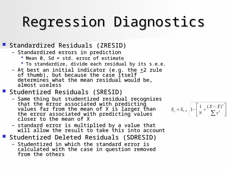
Regression DiagnosticsRegression Diagnostics Standardized Residuals (ZRESID)Standardized Residuals (ZRESID)
– Standardized errors in predictionStandardized errors in prediction Mean 0, Sd = std. error of estimateMean 0, Sd = std. error of estimate To standardize, divide each residual by its s.e.e.To standardize, divide each residual by its s.e.e.
– At best an initial indicator (e.g. the At best an initial indicator (e.g. the ++2 rule of 2 rule of thumb), but because the case itself determines thumb), but because the case itself determines what the mean residual would be, almost uselesswhat the mean residual would be, almost useless
Studentized Residuals (SRESID)Studentized Residuals (SRESID)– Same thing but studentized residual recognizes Same thing but studentized residual recognizes
that the error associated with predicting values far that the error associated with predicting values far from the mean of X is larger than the error from the mean of X is larger than the error associated with predicting values closer to the associated with predicting values closer to the mean of X mean of X
– standard error is multiplied by a value that will standard error is multiplied by a value that will allow the result to take this into accountallow the result to take this into account
Studentized Deleted Residuals (SDRESID)Studentized Deleted Residuals (SDRESID)– Studentized in which the standard error is Studentized in which the standard error is
calculated with the case in question removed from calculated with the case in question removed from the othersthe others
Regression DiagnosticsRegression Diagnostics Mahalanobis’ DistanceMahalanobis’ Distance
– Mahalanobis distance is the distance of a case from the Mahalanobis distance is the distance of a case from the centroid of the remaining points (point where the means meet centroid of the remaining points (point where the means meet in n-dimensional space)in n-dimensional space)
Cook’s DistanceCook’s Distance– Identifies an influential data point whether in terms of Identifies an influential data point whether in terms of
predictor or DVpredictor or DV– A measure of how much the residuals of all cases would A measure of how much the residuals of all cases would
change if a particular case were excluded from the calculation change if a particular case were excluded from the calculation of the regression coefficients. of the regression coefficients.
– With larger (relative) values, excluding a case would change With larger (relative) values, excluding a case would change the coefficients substantially. the coefficients substantially.
DfBetaDfBeta– Change in the regression coefficient that results from the Change in the regression coefficient that results from the
exclusion of a particular case exclusion of a particular case – Note that you get DfBetas for each coefficient associated with Note that you get DfBetas for each coefficient associated with
the predictorsthe predictors
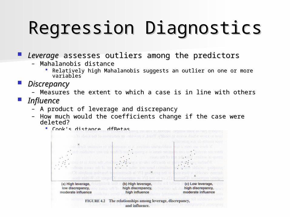
Regression DiagnosticsRegression Diagnostics LeverageLeverage assesses outliers among the predictors assesses outliers among the predictors
– Mahalanobis distance Mahalanobis distance Relatively high Mahalanobis suggests an outlier on one or more variablesRelatively high Mahalanobis suggests an outlier on one or more variables
DiscrepancyDiscrepancy– Measures the extent to which a case is in line with othersMeasures the extent to which a case is in line with others
InfluenceInfluence– A product of leverage and discrepancyA product of leverage and discrepancy– How much would the coefficients change if the case were deleted?How much would the coefficients change if the case were deleted?
Cook’s distance, dfBetasCook’s distance, dfBetas
OutliersOutliers
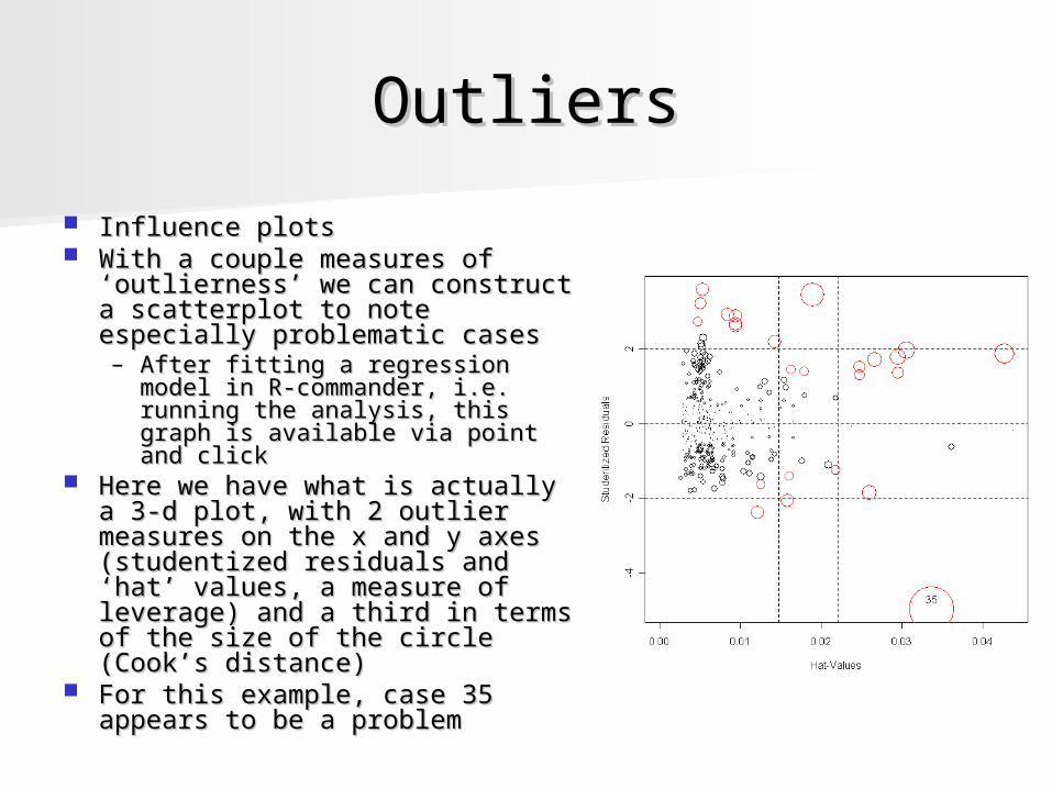
Influence plotsInfluence plots With a couple measures of With a couple measures of
‘outlierness’ we can construct a ‘outlierness’ we can construct a scatterplot to note especially scatterplot to note especially problematic cases problematic cases – After fitting a regression model After fitting a regression model
in R-commander, i.e. running in R-commander, i.e. running the analysis, this graph is the analysis, this graph is available via point and clickavailable via point and click
Here we have what is actually a Here we have what is actually a 3-d plot, with 2 outlier 3-d plot, with 2 outlier measures on the x and y axes measures on the x and y axes (studentized residuals and ‘hat’ (studentized residuals and ‘hat’ values, a measure of leverage) values, a measure of leverage) and a third in terms of the size and a third in terms of the size of the circle (Cook’s distance)of the circle (Cook’s distance)
For this example, case 35 For this example, case 35 appears to be a problemappears to be a problem
OutliersOutliers
It should be clear to interested readers It should be clear to interested readers whatever has been done to deal with whatever has been done to deal with outliersoutliers
Use appropriate software to perform Use appropriate software to perform robust regression (e.g. least trimmed robust regression (e.g. least trimmed squares) and compare and contrast the squares) and compare and contrast the results with classical approachesresults with classical approaches– Applications such as S-plus, R, and even SAS Applications such as S-plus, R, and even SAS
and Stata provide methods of robust and Stata provide methods of robust regression analysisregression analysis
Summary: OutliersSummary: Outliers No matter the analysis, some cases will be the No matter the analysis, some cases will be the
‘most extreme’. However, none may really ‘most extreme’. However, none may really qualify as being overly influential.qualify as being overly influential.
Whatever you do, always run some diagnostic Whatever you do, always run some diagnostic analysis and do not ignore influential casesanalysis and do not ignore influential cases
It should be clear to interested readers It should be clear to interested readers whatever has been done to deal with outlierswhatever has been done to deal with outliers
As noted before, the best approach to dealing As noted before, the best approach to dealing with outliers when they do occur is to run a with outliers when they do occur is to run a robust regression with capable softwarerobust regression with capable software
Suppressor variablesSuppressor variables There are a couple of ways in which suppression can occur There are a couple of ways in which suppression can occur
or be talked of, but the gist is that this masks the impact the or be talked of, but the gist is that this masks the impact the predictor would have on the dependent if the third variable predictor would have on the dependent if the third variable did not existdid not exist
In general suppression occurs when In general suppression occurs when ii falls outside the range falls outside the range of 0 of 0 rryiyi
Suppression in MR can entail some different relationships Suppression in MR can entail some different relationships among IVsamong IVs– For example one suppressor relationship would be where two For example one suppressor relationship would be where two
variables, Xvariables, X11 and X and X22, are positively related to Y, but when the , are positively related to Y, but when the equation comes out we getequation comes out we get
Y-hat = bY-hat = b11XX11 – b – b22XX22 + a + a
Three kinds to be discussedThree kinds to be discussed– ClassicalClassical– NetNet– CooperativeCooperative
SuppressionSuppression
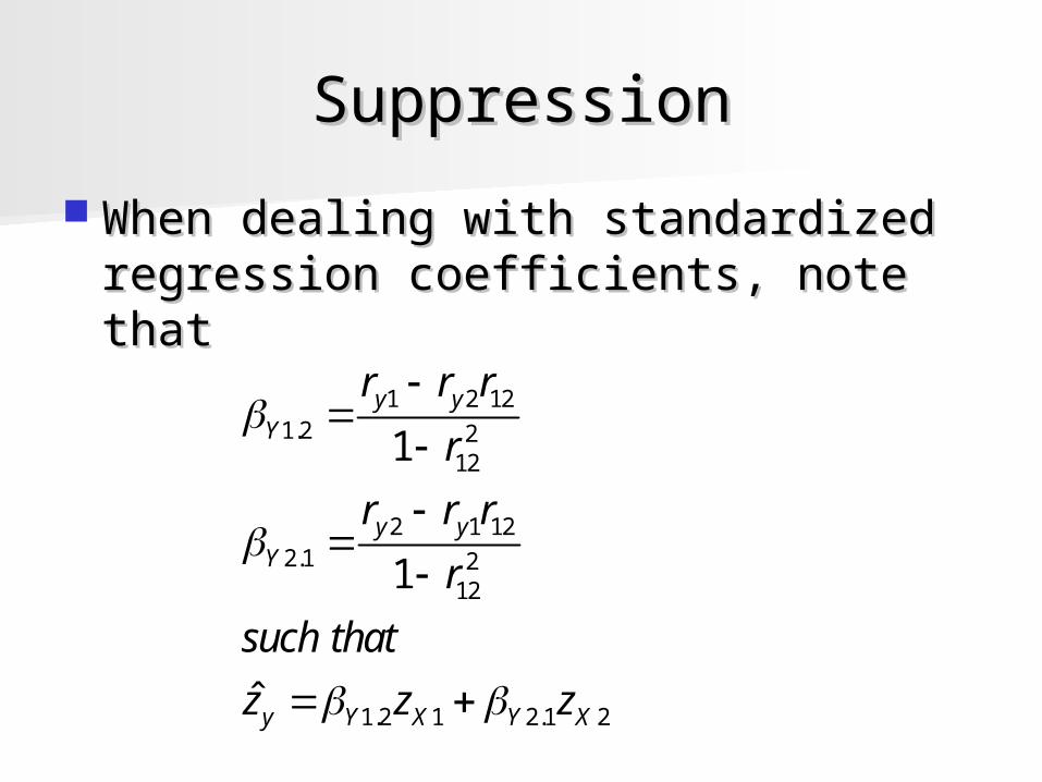
When dealing with standardized When dealing with standardized regression coefficients, note that regression coefficients, note that
1 2 121.2 2
12
2 1 122.1 2
12
1.2 1 2.1 2
1
1
ˆ
y yY
y yY
y Y X Y X
r r r
r
r r r
r
such that
z z z
SuppressionSuppression
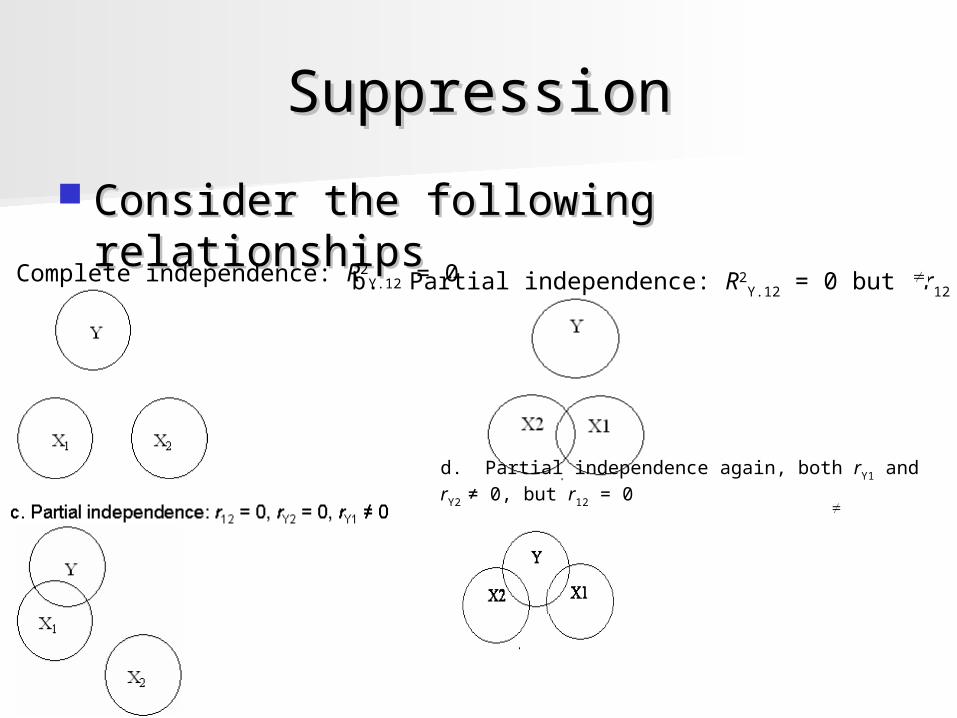
Consider the following relationshipsConsider the following relationships
a. Complete independence: R2Y.12 = 0
b. Partial independence: R2Y.12 = 0 but r12 0,
d. Partial independence again, both rY1 and rY2 ≠ 0, but r12 = 0
SuppressionSuppression
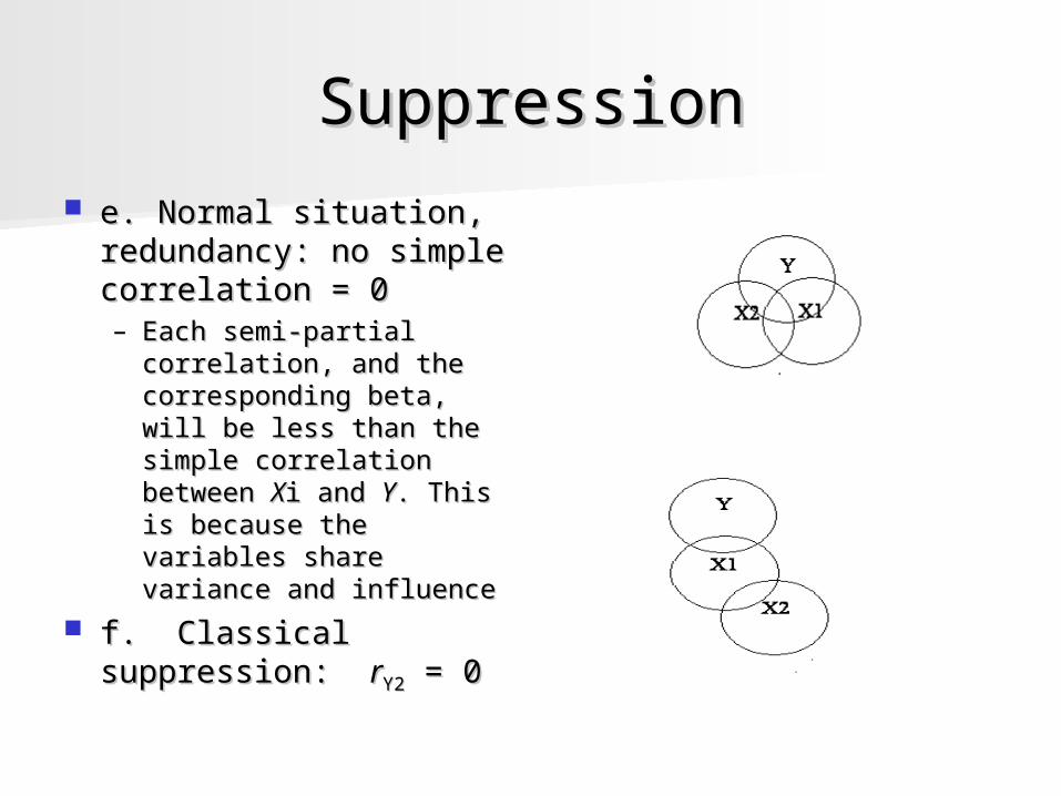
e. Normal situation, e. Normal situation, redundancy: no simple redundancy: no simple correlation = 0correlation = 0– Each semi-partial Each semi-partial
correlation, and the correlation, and the corresponding beta, will corresponding beta, will be less than the simple be less than the simple correlation between correlation between XXi i and and YY. This is because . This is because the variables share the variables share variance and influencevariance and influence
f. Classical f. Classical suppression: suppression: rrY2Y2 = 0 = 0
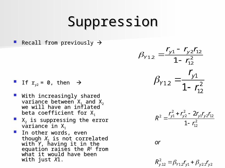
SuppressionSuppression Recall from previously Recall from previously
If rIf ry2 y2 = 0, then = 0, then
With increasingly shared With increasingly shared variance between Xvariance between X11 and X and X22 we will have an inflated beta we will have an inflated beta coefficient for Xcoefficient for X11
XX22 is suppressing the error is suppressing the error variance in Xvariance in X11
In other words, even though In other words, even though XX22 is not correlated with is not correlated with YY, , having it in the equation having it in the equation raises the raises the RR22 from what it from what it would have been with just would have been with just XX1. 1.
1 2 121.2 2
121y y
Y
r r r
r
11.2 2
121y
Y
r
r
2 21 2 1 2 122
212
2.12 1.2 1 2.1 2
2
1y y y y
y Y y y y
r r r r rR
r
or
R r r
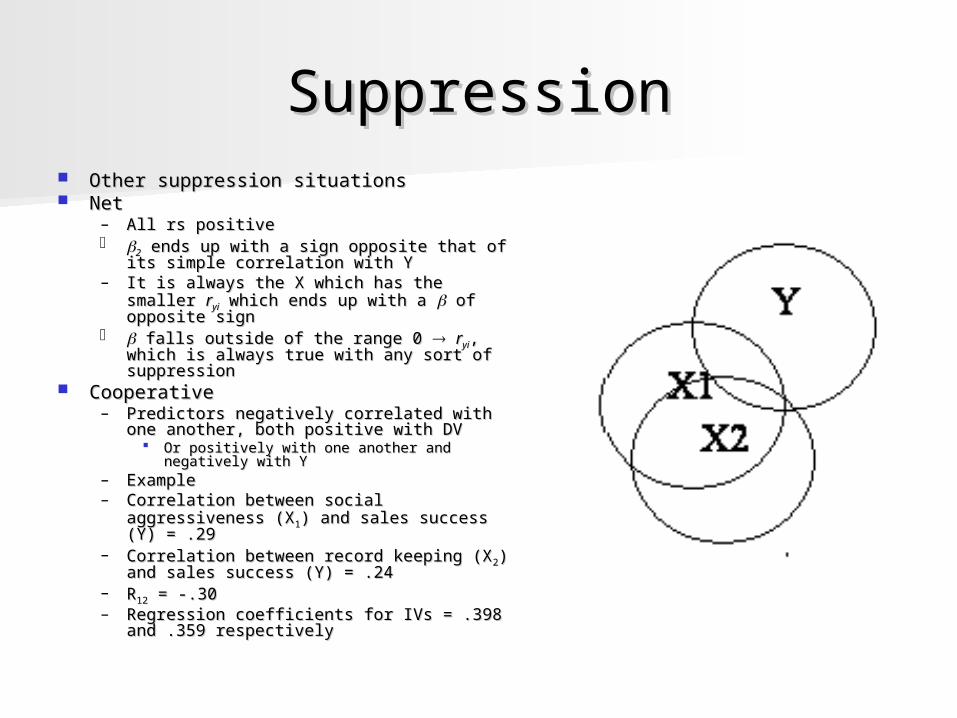
SuppressionSuppression Other suppression situationsOther suppression situations NetNet
– All rs positiveAll rs positive 22 ends up with a sign opposite that of its ends up with a sign opposite that of its
simple correlation with Y simple correlation with Y – It is always the X which has the smaller It is always the X which has the smaller rryiyi
which ends up with a which ends up with a of opposite sign of opposite sign falls outside of the range 0 falls outside of the range 0 rryiyi, which , which
is always true with any sort of is always true with any sort of suppressionsuppression
CooperativeCooperative– Predictors negatively correlated with one Predictors negatively correlated with one
another, both positive with DVanother, both positive with DV Or positively with one another and Or positively with one another and
negatively with Ynegatively with Y– ExampleExample– Correlation between social Correlation between social
aggressiveness (Xaggressiveness (X11) and sales success (Y) ) and sales success (Y) = .29= .29
– Correlation between record keeping (XCorrelation between record keeping (X22) ) and sales success (Y) = .24and sales success (Y) = .24
– RR1212 = -.30 = -.30– Regression coefficients for IVs = .398 and Regression coefficients for IVs = .398 and
.359 respectively.359 respectively
SuppressionSuppression
*For statistically significant IVs
Gist: weird stuff can happen in MR, so Gist: weird stuff can happen in MR, so take note of the relationship of the IVs take note of the relationship of the IVs and how it may affect your overall and how it may affect your overall interpretationinterpretation
Compare the simple correlations of Compare the simple correlations of each IV with the DV and compare to each IV with the DV and compare to their respective beta coefficients*their respective beta coefficients*– If coefficient noticeably larger than simple If coefficient noticeably larger than simple
correlation (absolute value) or of opposite correlation (absolute value) or of opposite sign one should suspect possible sign one should suspect possible suppressionsuppression
Model ValidationModel Validation
OverfittingOverfitting ValidationValidation BootstrappingBootstrapping
OverfittingOverfitting
External validityExternal validity In some cases, some of the variation the In some cases, some of the variation the
parameters chosen are explaining is parameters chosen are explaining is variation that is idiosyncratic to the samplevariation that is idiosyncratic to the sample– We would not see this variability in the populationWe would not see this variability in the population
So the fit of the model is good, but it doesn’t So the fit of the model is good, but it doesn’t generalize as well as one would thinkgeneralize as well as one would think
Capitalization on chanceCapitalization on chance
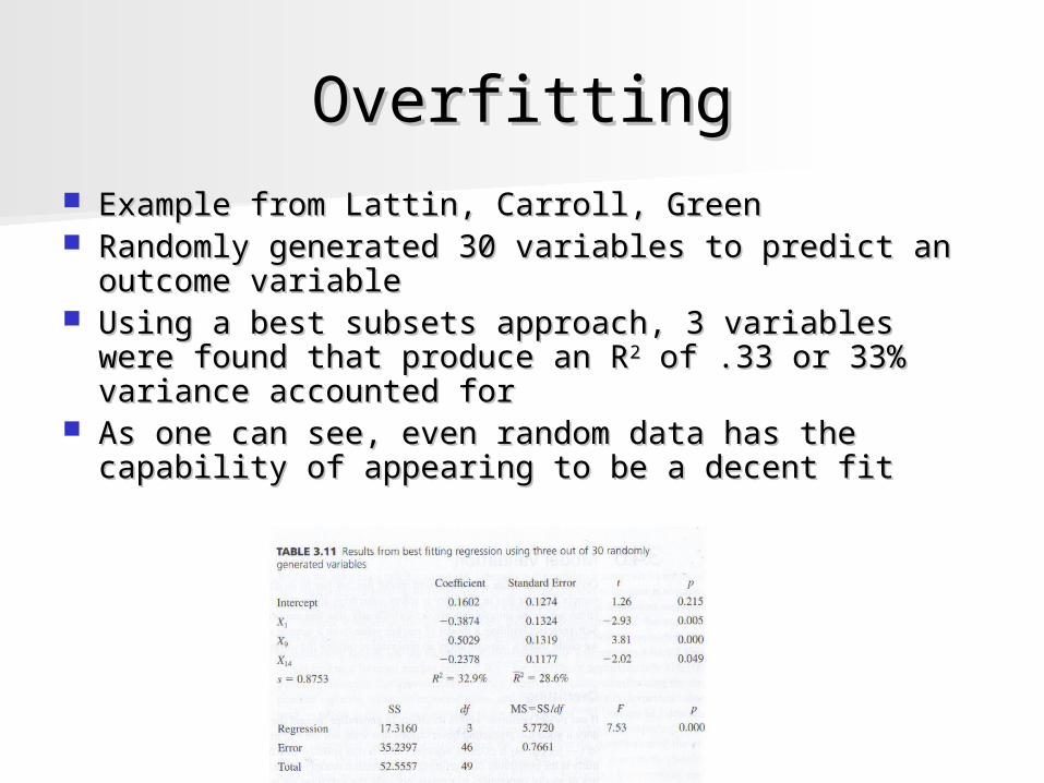
OverfittingOverfitting Example from Lattin, Carroll, GreenExample from Lattin, Carroll, Green Randomly generated 30 variables to predict an Randomly generated 30 variables to predict an
outcome variableoutcome variable Using a best subsets approach, 3 variables were Using a best subsets approach, 3 variables were
found that produce an Rfound that produce an R22 of .33 or 33% variance of .33 or 33% variance accounted foraccounted for
As one can see, even random data has the As one can see, even random data has the capability of appearing to be a decent fit capability of appearing to be a decent fit
ValidationValidation One way to deal with such a problem is with a simple One way to deal with such a problem is with a simple
random splitrandom split With large datasets one can randomly split the sample into With large datasets one can randomly split the sample into
two setstwo sets– Calibration sample: used to estimate the coefficientsCalibration sample: used to estimate the coefficients– Holdout sample: used to validate the modelHoldout sample: used to validate the model
Some suggest a 2:1 or 4:1 splitSome suggest a 2:1 or 4:1 split Using the coefficients from the calibration set one can Using the coefficients from the calibration set one can
create predicted values for the holdout setcreate predicted values for the holdout set The squared correlation between the predicted values and The squared correlation between the predicted values and
observed values can then be compared to the Robserved values can then be compared to the R2 2 of the of the calibration setcalibration set
In previous example of randomly generated data the RIn previous example of randomly generated data the R22 for for the holdout set was 0the holdout set was 0
Other approachesOther approaches Jackknife ValidationJackknife Validation
– Create estimates with a particular case removedCreate estimates with a particular case removed– Use the coefficients obtained from analysis of the n-1 Use the coefficients obtained from analysis of the n-1
remaining cases to create a predicted value for the remaining cases to create a predicted value for the case removedcase removed
– Do for all cases, and then compare the jackknifed RDo for all cases, and then compare the jackknifed R22 to the originalto the original
Subsets approachSubsets approach– Create several samples of the data of roughly equal Create several samples of the data of roughly equal
sizesize– Use the holdout approach with one sample, and Use the holdout approach with one sample, and
obtain estimates from the othersobtain estimates from the others– Do this for each sample, obtain average estimatesDo this for each sample, obtain average estimates
BootstrapBootstrap
With relatively smaller samples*, cross-With relatively smaller samples*, cross-validation may not be as feasiblevalidation may not be as feasible
One may instead resample (with One may instead resample (with replacement) from the original data to replacement) from the original data to obtain estimates for the coefficientsobtain estimates for the coefficients– Use what is available to create a Use what is available to create a
sampling distribution of for the values of sampling distribution of for the values of interestinterest
* but still large enough such that the bootstrap estimates would be viablebut still large enough such that the bootstrap estimates would be viable
SummarySummary
There is a lot to consider when There is a lot to consider when performing multiple regression performing multiple regression analysisanalysis
Actually running the analysis is just Actually running the analysis is just the first step, and if that’s all we are the first step, and if that’s all we are doing, we haven’t done muchdoing, we haven’t done much
A lot of work will be necessary to A lot of work will be necessary to make sure that the conclusions drawn make sure that the conclusions drawn will be worthwhilewill be worthwhile
And that’s ok, you can do it!And that’s ok, you can do it!
Recommended