Modeling Model Uncertainty
Alexei Onatski
Department of Economics
Columbia University
e-mail: [email protected]
Noah Williams∗
Department of Economics
Princeton University and NBER
e-mail: [email protected]
April 4, 2003
Abstract
Recently there has been a great deal of interest in studying monetary policy under
model uncertainty. We point out that different assumptions about the uncertainty may
result in drastically different “robust” policy recommendations. Therefore, we develop
new methods to analyze uncertainty about the parameters of a model, the lag specifi-
cation, the serial correlation of shocks, and the effects of real time data in one coherent
structure. We consider both parametric and nonparametric specifications of this struc-
ture and use them to estimate the uncertainty in a small model of the US economy.
We then use our estimates to compute robust Bayesian and minimax monetary policy
rules, which are designed to perform well in the face of uncertainty. Our results suggest
that the aggressiveness recently found in robust policy rules is likely to be caused by
overemphasizing uncertainty about economic dynamics at low frequencies.
JEL Classification: E52, C32, D81.
∗The original version of this paper was prepared for the 2002 ISOM in Frankfurt. We thank the participantsin the seminar, especially our discussants Glenn Rudebusch and Ulf Soderstrom for detailed and insightfuldiscussions and Chris Sims for useful comments. We are extremely grateful to Jim Stock for inviting us toparticipate and for providing helpful comments. We also thank Glenn Rudebusch and Athanasios Orphanidesfor providing us with data. Finally, we thank the editor, Roberto Perotti, and three anonymous referees forcomments and suggestions that greatly improved the substance and presentation of the paper. Alexei Onatskithanks Columbia University for providing a financial support in the form of a Council Grant for summerresearch.
1
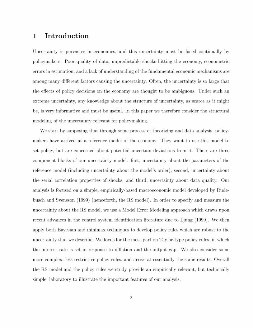
1 Introduction
Uncertainty is pervasive in economics, and this uncertainty must be faced continually by
policymakers. Poor quality of data, unpredictable shocks hitting the economy, econometric
errors in estimation, and a lack of understanding of the fundamental economic mechanisms are
among many different factors causing the uncertainty. Often, the uncertainty is so large that
the effects of policy decisions on the economy are thought to be ambiguous. Under such an
extreme uncertainty, any knowledge about the structure of uncertainty, as scarce as it might
be, is very informative and must be useful. In this paper we therefore consider the structural
modeling of the uncertainty relevant for policymaking.
We start by supposing that through some process of theorizing and data analysis, policy-
makers have arrived at a reference model of the economy. They want to use this model to
set policy, but are concerned about potential uncertain deviations from it. There are three
component blocks of our uncertainty model: first, uncertainty about the parameters of the
reference model (including uncertainty about the model’s order); second, uncertainty about
the serial correlation properties of shocks; and third, uncertainty about data quality. Our
analysis is focused on a simple, empirically-based macroeconomic model developed by Rude-
busch and Svensson (1999) (henceforth, the RS model). In order to specify and measure the
uncertainty about the RS model, we use a Model Error Modeling approach which draws upon
recent advances in the control system identification literature due to Ljung (1999). We then
apply both Bayesian and minimax techniques to develop policy rules which are robust to the
uncertainty that we describe. We focus for the most part on Taylor-type policy rules, in which
the interest rate is set in response to inflation and the output gap. We also consider some
more complex, less restrictive policy rules, and arrive at essentially the same results. Overall
the RS model and the policy rules we study provide an empirically relevant, but technically
simple, laboratory to illustrate the important features of our analysis.
2

Recently there has been a great deal of research activity on monetary policy making
under uncertainty. Unfortunately, the practical implications of this research turn out to be
very sensitive to different assumptions about uncertainty. For example, the classic analysis of
Brainard (1967) showed that uncertainty about the parameters of a model may lead to cautious
policy. More recently, Sargent (1999) showed that the introduction of extreme uncertainty
about the shocks in the Ball (1999) model implies that very aggressive policy rules may
be optimal. On the contrary, Rudebusch (2001) shows that focusing on the real time data
uncertainty in the conceptually similar RS model leads to the attenuation of the optimal
policy rule. Further, Craine (1979) and Soderstrom (2002) show that uncertainty about the
dynamics of inflation leads to aggressive policy rules. Finally, Onatski and Stock (2002) find
that uncertainty about the lag structure of the RS model requires a cautious reaction to
inflation, but an aggressive response to variation in the output gap.
The fact that the robust policy rules are so fragile with respect to different assumptions
about the structure of uncertainty is not surprising by itself. Fragility is a general feature of
optimizing models. Standard stochastic control methods are robust to realizations of shocks,
as long as they come from the assumed distributions and feed through the model in the
specified way. But the optimal rules may perform poorly when faced with a different shock
distribution, or slight variation in the model. The policy rules discussed above are designed
to be robust to a particular type of uncertainty, but may perform poorly when faced with
uncertainty of a different nature. In our view, the most important message of the fragility of
the robust rules is that to design a robust policy rule in practice, it is necessary to combine
different sources of uncertainty in a coherent structure and carefully estimate or calibrate the
size of the uncertainty. In other words, we must structurally model uncertainty.
As described above, we assume that policymakers start with a reference model of the
economy. At a general level, model uncertainty can be adequately represented by suitable
special restrictions on the reference model’s shocks. For example, if one is uncertain about
3

the parameters of the reference model or whether all relevant variables were included in the
model, one should suspect that the reference shocks might actually be correlated with the
explanatory variables in the model. That is, the reference model’s shocks would now include
“true” exogenous shocks and modeling errors. The model uncertainty can be formulated by
defining a set of potentially true models for these errors, or by “Model Error Modeling.”
One popular way to describe restrictions on the reference shocks (see for example Hansen
and Sargent (2002)) is to assume that the shocks must be of bounded size, but arbitrary
otherwise. We argue that a much more structured model of the shocks must be used to
describe uncertainty relevant to monetary policymaking. In particular, we develop an example
showing that the Hansen and Sargent (2002) approach may lead to the design of robust policy
rules that can be destabilized by small parametric perturbations. Thus while the robust rule
may resist shocks of a certain size, small variations in the underlying model can result in
disastrous policy performance.
We then turn to the task of formulating an empirical description of uncertainty by model
error modeling. In particular, we discuss and implement both parametric and nonparametric
specifications for the RS model errors. The parametric specification imposes more structure
and results in a probabilistic description of uncertainty. We estimate these parameters using
Bayesian methods, obtaining a posterior distribution which characterizes the uncertainty.
The nonparametric specification imposes fewer restrictions, and results in a deterministic
specification of the uncertainty. This allows us to calibrate the size of the uncertainty set, but
as it is a deterministic description, we cannot evaluate the likelihood of alternative models in
the set.
After we estimate or calibrate the uncertainty, we use our results to formulate robust policy
rules which are designed to work well for the measured uncertainty. From the parametric
specification, we have a distribution over possible models. Therefore for this specification
we find robust optimal rules which minimize the Bayesian risk. From the nonparametric
4

specification, we have bounds on the uncertainty set. Therefore for this specification we
find robust optimal rules which minimize the worst possible loss for the models in the set.
This minimax approach follows much of the recent literature on robust control, and provides a
tractable way of using our most general uncertainty descriptions. While there is the possibility
that minimax results may be driven by unlikely models, we focus solely on empirically plausible
model perturbations. Further, for many of our specifications the Bayesian and minimax results
are quite similar. This suggests both that the stronger restrictions in the Bayesian framework
do not greatly affect results, and that the minimax results are not driven by implausible worst
case scenarios. It is worth noting that in all of our results we assume that policy makers
commit to a rule once-and-for-all. Although this approach is common in the literature, it
is clearly an oversimplification. This should be kept in mind, particularly when considering
some of the bad outcomes we find for certain policy rules.
Without imposing much prior structure on the model perturbations, the parametric-
Bayesian analysis finds some attenuation in policy. This is keeping with the Brainard (1967)
intuition. However our nonparametric-minimax analysis finds that dynamic instability is a
possibility for any policy rule. This suggests the potential for very large losses and very poor
economic performance when policy is conducted using such interest rate rules. However when
we tighten prior beliefs so that instability is deemed unlikely, our results change rather sub-
stantially. In this case, the optimal rule from the Bayesian analysis is slightly more aggressive
than the optimal rule in the absence of model uncertainty. However our minimax optimal rule
is quite close to the no-uncertainty benchmark. But these rules remain relatively aggressive
in comparison with directly estimated policy rules.
Upon further inspection, we find that in many cases the most damaging model pertur-
bations come from very low frequency changes. Correspondingly, many of the robust policy
rules that we find are relatively aggressive, stemming from policymakers’ fears of particularly
bad long-run deviations from the RS model. In particular, we impose a vertical long-run
5
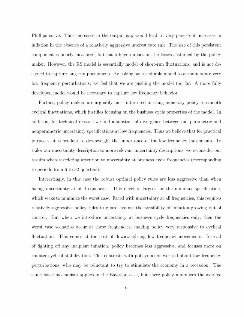
Phillips curve. Thus increases in the output gap would lead to very persistent increases in
inflation in the absence of a relatively aggressive interest rate rule. The size of this persistent
component is poorly measured, but has a huge impact on the losses sustained by the policy
maker. However, the RS model is essentially model of short-run fluctuations, and is not de-
signed to capture long-run phenomena. By asking such a simple model to accommodate very
low frequency perturbations, we feel that we are pushing the model too far. A more fully
developed model would be necessary to capture low frequency behavior.
Further, policy makers are arguably most interested in using monetary policy to smooth
cyclical fluctuations, which justifies focusing on the business cycle properties of the model. In
addition, for technical reasons we find a substantial divergence between our parametric and
nonparametric uncertainty specifications at low frequencies. Thus we believe that for practical
purposes, it is prudent to downweight the importance of the low frequency movements. To
tailor our uncertainty description to more relevant uncertainty descriptions, we reconsider our
results when restricting attention to uncertainty at business cycle frequencies (corresponding
to periods from 6 to 32 quarters).
Interestingly, in this case the robust optimal policy rules are less aggressive than when
facing uncertainty at all frequencies. This effect is largest for the minimax specification,
which seeks to minimize the worst case. Faced with uncertainty at all frequencies, this requires
relatively aggressive policy rules to guard against the possibility of inflation growing out of
control. But when we introduce uncertainty at business cycle frequencies only, then the
worst case scenarios occur at these frequencies, making policy very responsive to cyclical
fluctuation. This comes at the cost of downweighting low frequency movements. Instead
of fighting off any incipient inflation, policy becomes less aggressive, and focuses more on
counter-cyclical stabilization. This contrasts with policymakers worried about low frequency
perturbations, who may be reluctant to try to stimulate the economy in a recession. The
same basic mechanism applies in the Bayesian case, but there policy minimizes the average
6

loss across frequencies. Low frequency perturbations again imply more aggressive policy, but
these perturbations are given much less weight when choosing policy rules to minimize the
Bayesian risk. Thus the effects of removing low frequency perturbations is much smaller.
One of the main benefits of our approach is that it allows us to treat many different forms
of uncertainty in a unified framework. However it is also interesting to consider the different
sources independently. This allows us to see how the uncertainty channels affect policy rules,
and to determine which channels have the largest effects on losses. These results can provide
useful information for users of similar models, by pointing out the most important parts of the
model specification. Echoing our discussion of the fragility of robust rules above, we find that
the different channels have rather different effects. Uncertainty about the parameters and the
lag structure is likely the most important channel. It turns out that many of the empirically
plausible perturbations in this case make the model easier to control, so the resulting Bayesian
rules are attenuated and lead to smaller losses. However for all policy rules, we find that
instability is possible under our nonparametric calibration, suggesting a disastrous worst case.
We also find that real time data uncertainty may have significant effects on optimal policy
rules and their performance. When we restrict our attention to business cycle frequencies, we
again find that most of the policy rules become attenuated.
In the next section of the paper we describe the framework for our analysis at a gen-
eral level. In Section 3 we present an example highlighting the importance of the model
of uncertainty, and show that parametric and shock uncertainty must be considered sepa-
rately. Section 4 describes our application of the Model Error Modeling approach to find both
parametric and nonparametric measures of the uncertainty associated with the Rudebusch-
Svensson model. Section 5 formulates robust monetary policy rules based on our uncertainty
descriptions. Section 6 concludes.
7

2 General Framework
The general issue that we consider in this paper is decision making under model uncertainty.
In particular, we focus on the policy-relevant problem of choosing interest rate rules when the
true model of the economy is unknown and may be subject to different sources of uncertainty.
The goal of the paper is to provide characterizations of the empirically relevant sources of
uncertainty, and to design policy rules which account for that uncertainty.
The starting point of our analysis is a reference model of the economy:
xt+1 = A(L)xt + B1(L)ut + B2(L)εt (1)
yt = C(L)xt + D(L)εt, (2)
where xt is a vector of macroeconomic indicators, ut is a vector of controls such as taxes,
money, or interest rates, yt is a vector of variables observed in real time, εt is a vector of white
noise shocks, and A(L), Bi(L), C(L), and D(L) are matrix lag polynomials. Note that the
majority of purely backward-looking models of the economy can be represented in the above
form. In fact, by defining the state appropriately, this system of equations has a standard
state-space form. We consider this form of the reference model because, as will soon be clear,
it accords with our description of the uncertainty.
As mentioned in the introduction, we assume that through some unmodeled process of trial
and error policy makers have arrived at a reference model of the economy. In this paper, we
do not address an important question of how to choose a reference model. Instead, we assume
that the reference model is given, and policy makers are concerned about small deviations of
the true model from the reference one. This is also the starting point of much of the literature
on robustness in economics, as described for example in Hansen and Sargent (2002). A more
ambitious question of what policy a central bank should follow under vast disagreement about
8

the true model of the economy is addressed, for example in Levin, Wieland, and Williams
(1999).
We assume that policymakers have a time-additively separable quadratic loss function:
Lt = Et
∞∑i=0
βix′t+iΛxt+i.
They seek to minimize losses by choosing a policy rule from an admissible class:
ut = f(yt, yt−1, ..., ut−1, ut−2, ...).
The admissible class does not necessarily include the optimal control because the optimality
of a rule may be traded off with its other characteristics, such as simplicity. In some cases it
is more convenient to discuss policymakers maximizing a utility function, which is simply the
negative of the loss function.
Equations (1) and (2) can be estimated for a time period in the past for which both real-
time data yt, ut and the final data xt are available. The obtained estimates can then be used to
compute the best policy rule from the admissible class. The quality of the policy rule obtained
in this way will depend on the accuracy of the reference model. In general, this model will
not be completely accurate. The reference model is likely to be a stylized macroeconomic
model, which for tractability may leave out certain variables or focus only on the first few lags
of the relevant variables. While these simplifications may be justified for both practical and
statistical reasons, we will show that they can have a large impact on policy decisions.
We assume that a more accurate model of the economy encompasses the reference model
9

as follows:
xt+1 =(A(L) + A(L)
)xt +
(B1(L) + B1(L)
)ut +
(B2(L) + B2(L)
)εt (3)
yt =(C(L) + C(L)
)xt +
(D(L) + D(L)
)εt, (4)
where A(L), Bi(L), C(L) and D(L) are relatively unconstrained matrix lag polynomials of
potentially infinite order. Our assumption allows for a rich variety of potential defects in the
reference model. Econometric errors in the estimation of the reference parameters, misspecifi-
cations of the lag structure of the reference equations, and misinterpretations of the real-time
data are all considered as distinct possibilities.
We assume that the central bank wants to design a policy rule that works well not only
for the reference model but also for statistically plausible deviations from the reference model
having form (3,4). Formally, such a set can be defined by a number of restrictions R on the
matrix lag polynomials A(L), Bi(L), C(L) and D(L). The restrictions R may be deterministic
if sets of the admissible matrix lag polynomials are specified, or stochastic if distributions of
the polynomials’ parameters are given.
We formalize policy makers’ desire for robustness by assuming that they use Bayesian or
minimax strategy for choosing the policy, depending on whether R is stochastic or determin-
istic. That is, in the stochastic case policy makers solve the Bayes problem:
min{ut=f(·)}
ERLt (5)
where the expectation is taken with respect to distributions of the potential deviations from
the reference model specified byR. In the deterministic case, they solve the minimax problem:
min{ut=f(·)}
maxR
Lt (6)
10

where the maximum is taken over all matrix lag polynomials A(L), Bi(L), C(L) and D(L)
satisfying the deterministic restrictions R.1
It is needless to say that, at least in principle, the particular structure of the restrictions
R will strongly affect solutions to the above problems. In the next section, we illustrate
importance of this structure through a simple example.
3 Consequences of Different Uncertainty Models
It is useful to re-write (3)-(4) to represent the model uncertainty in the form:
xt+1 = A(L)xt + B1(L)ut + wt
yt = C(L)xt + st,
where we define the “model errors” as:
wt = A(L)xt + B1(L)ut +(B2(L) + B2(L)
)εt, (7)
st = C(L)xt +(D(L) + D(L)
)εt,
and A(L), Bi(L), C(L) and D(L) comply with R. This representation shows that, the uncer-
tainty may be described by restrictions (7) on the model errors wt and st.
One approach to model uncertainty, similar in spirit to that developed by Hansen and
Sargent (2002), does not impose any special structure on wt and st. Instead, the approach
1Note that in our formulation, the model uncertainty takes form of a one-time uncertain shift in theparameters or specification of the reference model. For an analysis of uncertainty interpreted as a stochasticprocess in the space of models see Rudebusch (2001).
11

considers all errors subject to the restriction:
E
∞∑t=0
βt(w′tΦ1wt + s′tΦ2st) ≤ η. (8)
The parameter η in the above inequality regulates the size of uncertainty, and it may be
calibrated so that the corresponding deviations from the reference model are statistically
plausible. While this approach seems quite general and unrestrictive, not taking into account
the particular structure of wt and st may seriously mislead decision makers. We now develop
an example illustrating this fact. The example considers a practically important situation,
although in later sections we slightly change the policy rules and the loss function we consider.
We consider a two-equation purely backward-looking model of the economy proposed and
estimated by Rudebusch and Svensson (1999). This model is the benchmark for the rest of
the paper as well, and is given by:
πt+1 = .70(.08)
πt − .10(.10)
πt−1 + .28(.10)
πt−2 + .12(.08)
πt−3 + .14(.03)
yt + επ,t+1 (9)
yt+1 = 1.16(.08)
yt − .25(.08)
yt−1 − .10(.03)
(ıt − πt) + εy,t+1
The standard errors of the parameter estimates are given in parentheses. Here the variable
y stands for the gap between output and potential output, π is inflation and i is the federal
funds rate. All the variables are quarterly, measured in percentage points at an annual rate
and demeaned prior to estimation, so there are no constants in the equations. The variables
π and i stand for four-quarter averages of inflation and the federal funds rate respectively.
The first equation is a simple version of the Phillips curve, relating the output gap and
inflation. The coefficients on the lags of inflation in the right hand side of the equation sum
to one, so that the Phillips curve is vertical in the long run. The second equation is a variant
of the IS curve, relating the real interest rate to the output gap. A policymaker can control
12

the federal funds rate and wants to do so in order to keep y and π close to their target values
(zero in this case). For the present, we ignore the real-time data issues so that our reference
model does not include equations describing real-time data generating process.
In general, the policy maker’s control policy may take the form of a contingency plan for
her future settings of the federal funds rate. Here we restrict attention to the Taylor-type
rules for the interest rate. As emphasized by McCallum (1988) and Taylor (1993), simple
rules have the advantage of being easy for policymakers to follow and easy to interpret. In
our analysis in later sections, we consider simple rules but we also analyze the performance
of feedback rules of a more general form. In this section, we assume that the policymaker
chooses among the following rules:
it = gππt−1 + gyyt−2 (10)
Here, the interest rate reacts to both inflation and the output gap with delay. The delay in the
reaction to the output gap is longer than that in the reaction to the inflation because it takes
more time to accurately estimate the gap. The timing in the above policy rule is unorthodox,
and is made here to sharpen our results. In later sections we use the more conventional timing,
in which the interest rate responds contemporaneously to inflation and the output gap, and
we also consider more general policy rules.
Following Rudebusch and Svensson (1999), we assume here that the policy maker has the
quadratic loss function:
Lt = π2t + y2
t +1
2(it − it−1)
2. (11)
The inclusion of the interest-smoothing term (it − it−1)2 in the loss function is somewhat
controversial. Our results will not depend on whether this term is included in the loss function
or not, but we keep it here to again sharpen our results. In later sections we assume, as in
13
Woodford (2002), that the loss function depends on the level of the interest rate, not the
changes in rates.
If the policy maker were sure that the model is correctly specified, she could use standard
methods to estimate the expected loss for any given policy rule (10). Then she could find the
optimal rule numerically. Instead, we assume that the policy maker has some doubts about
the model. She wants therefore to design her control so that it works well for reasonable
deviations from the original specification. One of the most straightforward ways to represent
her doubts is to assume that the model parameters may deviate from their point estimates
as, for example, is assumed in Brainard (1967). It is also likely, that the policy maker would
not rule out misspecifications of the model’s lag structure. As Blinder (1997) states, “Failure
to take proper account of lags is, I believe, one of the main sources of central bank error.”
For the sake of illustration, we assume that the policy maker contemplates the possibility
that one extra lag of the output gap in the Phillips curve and IS equations and one extra
lag of the real interest rate in the IS equation were wrongfully omitted from the original
model. She therefore re-estimates the Rudebusch-Svensson model with the additional lags.
The re-estimated model has the following form:
πt+1 = .70(.08)
πt − .10(.10)
πt−1 + .28(.10)
πt−2 + .12(.09)
πt−3 + .14(.10)
yt + .00(.10)
yt−1 + επ,t+1 (12)
yt+1 = 1.13(.08)
yt − .08(.12)
yt−1 − .14(.08)
yt−2 − .32(.14)
(ıt − πt) + .24(.14)
(ıt−1 − πt−1) + εy,t+1
Then she obtains the covariance matrix of the above point estimates and tries to design her
control so that it works best for the worst reasonable deviation of the parameters from the
point estimates. For example, she may consider all parameter values inside the 50 percent
confidence ellipsoid around the point estimates.2
2In the later sections of the paper we discuss a more systematic way of representing and estimating themodel uncertainty. We also do not restrict our attention to the minimax setting as we do in this section.
14

We will soon return to this problem, but for now let us give an alternative, less structured,
description of the uncertainty. In general, we can represent uncertainty by modeling the errors
w1t, w2t of the Phillips curve and the IS equations as any processes satisfying:
E
∞∑t=0
βt
(w2
1t
Var(επt)+
w22t
Var(εyt)
)< η.
Here we will consider the case β → 1. The special choice of the weights on errors to the
Phillips curve and the IS equations was made to accommodate the MATLAB codes that we
use in our calculations.
In the extreme case when η tends to infinity, our uncertainty will be very large, so the
corresponding robust (minimax) rule must insure the policy maker against a large variety
of deviations from the reference model. It can be shown that such an “extremely robust”
policy rule minimizes the so-called H∞ norm of the closed loop system transforming the noise
εt =(επt/
√Var(επt), εyt/
√Var(εyt)
)into the target variables zt =
(πt, yt, (it − it−1)/
√2)′
(see Hansen and Sargent (2002)). It is therefore easy to find such a rule numerically using, for
example, commercially available MATLAB codes to compute the H∞ norm. Our computations
give the following rule:
it = 3.10πt−1 + 1.41yt−2. (13)
Now let us return to our initial formulation of the problem. Recall that originally we wanted
to find a policy rule that works well for all deviations of the parameters of the re-estimated
model (12) inside a 50 percent confidence ellipsoid around the point estimates. Somewhat
surprisingly, the above “extremely robust” rule does not satisfy our original criterion for
robustness. In fact, it destabilizes the economy for deviations from the parameters’ point
estimates inside as small as a 20 percent confidence ellipsoid. More precisely, the policy rule
(13) results in infinite expected loss for the following perturbation of the Rudebusch-Svensson
15

(RS) model:
πt+1 = .68πt − .13πt−1 + .35πt−2 + .10πt−3 + .30yt − .15yt−1 + επ,t+1 (14)
yt+1 = 1.15yt − .07yt−1 − .18yt−2 − .51 (ıt − πt) + .41 (ıt−1 − πt−1) + εy,t+1.
Let us denote the independent coefficients of the above model, the re-estimated RS model
(12), and the original RS model as c, c1, and c0 respectively.3 Also, let V be the covariance
matrix of the coefficients in the re-estimated model (12). Then we have:
(c− c1)′V −1(c− c1) = 6.15
(c0 − c1)′V −1(c0 − c1) = 5.34.
Both numbers are smaller than the 20 percent critical value of the chi-squared distribu-
tion with 10 degrees of freedom. This may be interpreted as saying that both the original
Rudebusch-Svensson model and the perturbed model are statistically close to the encompass-
ing re-estimated model. In spite of this, the robust rule leads to disastrous outcomes.
Why does our “extremely robust” rule perform so poorly? It is not because other rules
do even worse. For example, we checked that (a version of) the Taylor (1993) rule it =
1.5πt−1 + 0.5yt−2 guarantees stability for at least all deviations inside a 60 percent confidence
ellipsoid. The rule (13) works so poorly simply because it was not designed to work well in such
a situation. To see this, note that our original description of the model uncertainty allowed
deviations of the slope of the IS curve from its point estimate. Therefore our ignorance about
this parameter is particularly influential under very aggressive control rules. It may even be
consistent with instability under such an aggressive rule. However no effects of this kind are
3Recall that the sum of coefficients on inflation in the Phillips curve is restricted to be equal to 1.We therefore exclude the coefficient on the first lag of inflation from the vector of independent coeffi-cients. Collecting our estimates, these are: c = (−.13, .35, .10, .30,−.15, 1.15,−.07,−.18,−.51, .41)′, c1 =(−.10, .28, .12, .14, .00, 1.13,−.08,−.14,−.32, .24)′, c0 = (−.10, .28, .12, .14, 0, 1.16,−.25, 0,−.10, 0)′.
16

allowed under the unstructured description of model uncertainty. The specific interaction
between the aggressiveness of policy rules and uncertainty about the slope of the IS curve is
not taken into account. This lack of structure in the uncertainty description turns out to be
dangerous because the resulting robust rule happens to be quite aggressive.
The example just considered should not be interpreted in favor of a particular description of
uncertainty. Instead, it illustrates that when designing robust policy rules, we must carefully
specify and thoroughly understand the model uncertainty that we are trying to deal with.
Robust policy rules may be fragile with respect to reasonable changes in the model uncertainty
specification. In the next sections, we therefore use a systematic approach based on model
error modeling to estimate the uncertainty about the Rudebusch-Svensson model introduced
above. Then we use our estimates of the model uncertainty to find interest rate rules which
perform well in the face of this uncertainty.
4 Model Error Modeling
As was shown in the previous section, model uncertainty can be reformulated in terms of
restrictions (7) on the errors of the reference model. Hence, to form an empirically relevant
description of the uncertainty, one should find a set of models having the form (7) which
are consistent with available data and prior beliefs. We now begin specifying the model
uncertainty model for our application.
4.1 Specifying the Uncertainty Models
We start by adding equations describing the real-time data to the Rudebusch and Svensson’s
reference model of the economy described in the previous section. Such an extension of
the reference model is important because the central bank’s policy must feedback on the
information available in real time. As emphasized by Orphanides (2001), there is a substantial
17

amount of uncertainty in such information. Initial estimates of GDP, and hence the deflator
and output gap, are typically revised repeatedly and the revisions may be substantial.
Our reference assumption is that the real-time data on inflation, π∗t , and the output gap,
y∗, are equal to noisy lagged actual data, and the noise has AR(1) structure. That is:
π∗t = πt−1 + ηπt , where ηπ
t = ρπηπt−1 + vπ
t
y∗t = yt−1 + ηyt , where ηy
t = ρyηyt−1 + vy
t .
The assumption of the AR(1) noise in the real-time data accords with previous studies (see
for example Orphanides (2001) and Rudebusch (2001)). The choice of timing in the above
equations is consistent with the fact that lagged final data predicts the real-time data better
than the current final data do. This is true at least for the sample of the real-time data on
the output gap and inflation for the period from 1987:1 to 1993:04 that we use, which was
kindly provided to us by Athanasios Orphanides from his 2001 paper.
Using the Rudebusch-Svensson data set kindly provided to us (some time ago) by Glenn
Rudebusch, we compute the errors of the RS Phillips curve, eπt+1, and the IS curve, ey
t+1. Using
Athanasios Orphanides’ data, we compute the errors of our reference model for the real-time
data on inflation, ed,πt , and the output gap ed,y
t .4 We then model the reference model’s errors
as follows:
eπt+1 = a(L)(πt − πt−1) + b(L)yt + επ
t+1, where επt+1 = c(L)επ
t + uπt+1
eyt+1 = d(L)yt + f(L)πt + g(L)it + εy
t+1, where εyt+1 = h(L)εy
t + uyt+1
ed,πt = k(L)πt + ηπ
t , where ηπt = m(L)ηπ
t−1 + vπt
ed,yt = n(L)yt + ηy
t , where ηyt = p(L)ηy
t−1 + vyt .
4In our terminology, the “errors” of the real-time data reference equations are simply π∗t−πt−1 and y∗t−yt−1.
18

Several structurally distinct misspecifications of the RS model are consistent with our
model of the errors. First, non-zero functions a, b, d, f, and g imply errors in the coefficients
and lag specifications in the reference Phillips curve and the IS equations. Note that the
econometric errors in the point estimates of the reference parameters are thus taken into
account. The misspecification of the reference lag structure may be interpreted literally (say,
more distant lags of the real interest rate have a direct non-trivial effect on the output gap), or
as indicating omission of important explanatory variables from the reference model. Second,
our inclusion of both inflation and the nominal interest rate in the model of the IS equation
error eyt+1 allows for the separation of the effect of real and nominal interest rates on the
output gap.5 Finally, non-zero functions c and h allow for rich serial correlation structure of
the shocks to the Phillips and IS curves.
Similarly, for the reference real-time data equations, non-zero functions m and p extend
the possible serial correlation structure of the noise η beyond the reference AR(1) assumption.
As to the functions k and n, they model the “news component” of the data revision process.6
To see this, note that the revisions π∗t −πt and y∗t −yt can be expressed in the form (k(L)−1+
L)πt + ηπt and (n(L)− 1 + L)yt + ηy
t respectively. The functions k and n are thus responsible
for the structure of the correlation between the final data and the revisions, which defines the
news component. Note that, as pointed out by Rudebusch (2001) and Swanson (2000), the
typical certainty equivalence result in linear-quadratic models does not in general apply to
real-time data uncertainty. Certainty equivalence applies when the estimates of the underlying
unobserved states are efficient, but not when there is inefficient noise in the data revision
process. Moreover, for our results below we focus on a restricted class of policy rules, either of
the simple Taylor-type or of a less restrictive class. The classic certainty equivalence results
apply to optimal rules which respond to all state variables (which in our case would include all
5We thank Glenn Rudebusch for suggesting this extension of the reference model.6See Mankiw and Shapiro (1986) for a discussion of news versus noise in the revisions of real-time data.
19

of the additional variables in the model error models). Thus even if there were no additional
noise in the data revisions, the coefficients of our policy rules may change in the presence of
this partial information.
One possible extension of our analysis would be to include additional variables in the
model errors. For example, it is not unreasonable to think that the true dynamics of inflation
and the output gap should depend on the real exchange rate. Our description of uncertainty
does allow for such a relationship, albeit an implicit one. In this paper, we deal with reduced
form models. Of course, uncertainty about the reduced form dynamics may correspond to a
deeper uncertainty about a background structural model that includes more variables than
just inflation and the output gap. However, we could potentially sharpen our estimates of
uncertainty by explicitly including “omitted” variables directly in the error model. We leave
such important extensions of our analysis for future research.
4.2 Estimating the Models
We have structured the compound model uncertainty faced by policymakers via the lag poly-
nomials a(L) through p(L) describing the dynamics of the model errors. The restrictions on
these polynomials may either be parametric or nonparametric. In this section we describe
one parametric and one nonparametric specification. We also describe a possible way of for-
mulating empirically relevant constraints for each specification. The parametric specification
imposes more structure, and allows us to determine a probability distribution over the class
of alternative models. The nonparametric specification imposes significantly less structure,
but only provides bounds on the class of feasible alternative models. Later when we use our
measures of model uncertainty for policy decisions, these differences will be crucial.
First, for the parametric case, we assume that a, b, c, d, f, g, and h (which affect the Phillips
and IS curve errors) are fourth order lag polynomials, and k,m, n, and p (which affect the
20

−0.5 −0.4 −0.3 −0.2 −0.1 0 0.1 0.2 0.3 0.4 0.5−1
−0.8
−0.6
−0.4
−0.2
0
0.2
0.4
0.6
0.8
1
b0
b 1
Figure 1: MCMC draws from the posterior distribution of b0 and b1.
real-time data errors) are second order lag polynomials. The choice of these particular orders
of the polynomials is rather ad hoc. Looking ahead, we will estimate the error model using
a relatively short sample of the real-time data errors and a longer sample of the RS errors.
Therefore, the polynomials describing the dynamics of the real-time data errors are chosen to
have smaller order than those for the RS model.
We estimate an empirically relevant “distribution of the uncertainty” using Bayesian esti-
mation methods. In particular, we sample from the posterior distributions of the coefficients
of a, b, c, . . . , p and the posterior distributions of the variances of the shocks u and v using the
algorithm of Chib and Greenberg (1994) based on Markov Chain Monte Carlo simulations.
We assume diffuse priors for all parameters and obtain six thousand draws from the posterior
distribution, dropping the first thousand draws to ensure convergence. In Figure 1 we show
the MCMC draws from the joint posterior density of the coefficients b0 and b1 on the zero’s
and the first degree of L respectively in the polynomial b(L). These parameters can roughly be
interpreted as measuring the error of the RS model’s estimates of the effect of the output gap
21

on inflation. The picture demonstrates that the RS model does a fairly good job in assessing
the size of the effect of a one time change in the output gap on inflation (as most of the points
on the graph are near the origin). However, there exist some chances that the effect is either
more spread out over the time or, vice versa, that the initial response of inflation overshoots
its long run level. Averaging the draws from the posterior, we can obtain the point estimates
a, b, c, ..., p of the parameters of our error model. We will need these estimates to calibrate the
non-parametric uncertainty restrictions that we now discuss.
Clearly, restricting the polynomials to be of this specific order may rule out some plausible
deviations from the reference model. Such an undesirable restrictiveness, together with the
absence of clear rules for determining the orders of the lag polynomials, calls for an alter-
native, non-parametric description of the uncertainty. For such a description, we allow the
polynomials a(L), ..., p(L) to be of infinite order. We interpret these polynomials as general
causal linear filters having absolutely summable coefficients, that is we assume:
a(L) =∞∑
j=0
ajLj, where
∞∑j=0
|aj| < ∞
b(L) =∞∑
j=0
bjLj, where
∞∑j=0
|bj| < ∞,
and so on.7
In general, any linear filter x(L) with absolutely summable coefficients is uniquely deter-
mined by the Fourier transform of its coefficients, called the transfer function of the filter:
Γx(ω) =∞∑
j=0
xje−iωj. (15)
7The requirement of absolute summability of the filters’ coefficients is not really necessary for our analysis.For the results in the rest of the paper to remain valid it is enough to assume that the linear filter preservethe stationarity of inputs. However, the absolute summability is a standard requirement (see, for example,Priestley (1981), Ch. 4), and we keep it here.
22

We specify the model uncertainty restrictions in terms of restrictions on the transfer functions
of the filters a(L), ..., p(L) as follows. For each frequency ω, we require that:
∣∣∣Γa(ω)− Γa(ω)∣∣∣ < Wa(ω), . . . ,
∣∣∣Γp(ω)− Γp(ω)∣∣∣ < Wp(ω) (16)
where Γi(ω) and Wi(ω) are some complex-valued and positive real-valued functions of fre-
quency, respectively. We interpret Γi(ω) as our best guess about the value of the transfer
function Γi(ω) and Wi(ω) as a frequency-dependent parameter regulating the size of our
uncertainty about Γi(ω). Geometrically, the inequalities (16) restrict possible values of the
transfer functions Γi(ω) to lie in circles in the complex plane centered at Γi(ω) and having
radius Wi(ω).
The model uncertainty described by the inequalities (16 ) takes a form of the deterministic
set of models alternative to the reference model. Such a set can be made small if the weights
Wi are chosen to be small. Indeed, the uncertainty set can be reduced to a singleton if
Wi = 0. On the contrary, if the Wi are large, then the set is big, and therefore the amount of
uncertainty about the reference model is large.
To calibrate our non-parametric description of the uncertainty to an empirically relevant
size, we use the following strategy. At each frequency point ω, a rough idea about the possible
values of the transfer functions Γa(ω), . . . , Γp(ω) can be obtained by plotting a cloud of the
MCMC draws of the parametric versions of a(z), ..., p(z) evaluated at e−iω. Therefore, we
define our best guesses about the transfer functions at that frequency as:
Γa(ω) = a(e−iω), . . . , Γp(ω) = p(e−iω)
where a, . . . , p are the point estimates of the parametric specification of the polynomials defined
earlier in this section. Next, we calibrate Wa(ω), . . . , Wp(ω) so that the circles in the complex
23

plane with centers Γa(ω), . . . , Γp(ω) and radiuses Wa(ω), . . . , Wp(ω) include 50 percent of the
MCMC draws of (the parametric versions of) a(eiω), . . . , p(eiω). The 50 percent cutoff value
is arbitrary and can be adjusted, but we choose it to focus solely on plausible values of model
uncertainty.
Note that a specific choice of transfer functions satisfying (16) may be very different
from the sampled (parametric) transfer functions. In particular, although the frequency-by-
frequency analysis has a cutoff value of 50 percent, any resulting filter pieced together across
frequencies may have a much smaller likelihood of being observed. Even more important,
in our non-parametric description of the uncertainty we discard information about possible
correlations between a(eiω), . . . , p(eiω) and consider the direct product of the 50 percent re-
gions for a, ..., p. This may ”inflate” the uncertainty dramatically. However this method does
provide a tractable, implementable way of capturing model uncertainty without imposing a
great deal of a priori structure on the dynamics of the possible models. This generality is a
benefit of the approach, and is absent from the parametric case we considered above.
To summarize, the greater generality of the above non-parametric description of the uncer-
tainty comes with two big costs. First, a probabilistic description of uncertainty is substituted
by a deterministic description. Second, the deterministic uncertainty set may include some
irrelevant models because the calibration procedure proposed above is too crude. The latter
cost can be reduced by introducing more careful calibration techniques which is an important
topic left for the future research. In the next section, we show how to the use of our measures
of uncertainty to set policy.
5 The Robustness of Policy Rules
In the previous section we constructed both parametric and nonparametric model uncertainty
sets for the RS model. We now use Bayesian and minimax techniques to analyze the robustness
24

of Taylor-type rules, and we develop policy rules which are optimal in presence of the estimated
uncertainty.
5.1 Bayesian Analysis
In this section, we numerically solve the Bayesian problem (5), using our estimates of the
parametric uncertainty. Before proceeding, we must address the issue of the loss function.
Since we do not put restrictions on our priors, the posterior distribution of the coefficients
does not have finite support. Moreover, in our estimates we typically find non-negligible
probability that the system will be dynamically unstable. Therefore if we use the typical
quadratic loss (as in RS), non-zero mass will be assigned to infinite loss and any rule will
correspond to infinite Bayesian risk. One solution to this problem is to restrict our priors to
rule out instability and infinite losses. Another solution, which we choose, is to make the loss
function bounded from above. Clearly, the standard quadratic loss functions are only justified
as a local approximation of the true, non-quadratic loss (see Woodford (2002) for example).
Thus there is danger in extrapolating too far away from the mean, and it is not clear that the
same loss functions are relevant in extremely bad times. Moreover, bounded utility functions
and losses help to avoid the so-called St. Petersburg paradox in which individuals would risk
all of their wealth on a repeated coin toss lottery (see Mas-Colell, Whinston, and Green (1995)
for a discussion).
We now also drop the interest smoothing objective from the loss function, and instead
suppose that the loss is quadratic in the level of the interest rate.8 Woodford (2002) derives
a loss function of this form, where the interest rate penalization reflects the zero lower bound
on nominal interest rates and/or increased distortions associated with higher nominal rates.
8An earlier version of the paper considered a loss function with a smoothing objective. This did notsubstantially change the results. With a preference for smoothing, the overall level of the loss was higher, butthere was no significant alteration in the relative performance of different policy rules.
25

Optimal Rule CoefficientsPrior Rule Inflation Out. Gap Lagged Rates RiskType Type gπ0 gπ1 gπ2 gπ3 gy0 gy1 gi1 gi2 gi3
Unin. Complex 0.74 0.77 0.19 0.25 0.30 0.01 0.01 -0.15 -0.05 32.0Unin. Simple 1.75 0.25 - 36.0In. Complex 1.28 0.59 0.67 0.21 1.37 -0.33 0.09 -0.09 -0.01 29.0In. Simple 2.75 1.25 - 29.7
Table 1: The coefficients of the robust optimal Bayesian rules and corresponding Bayesian risk, for both thecomplex rules (18) and Taylor-type rules (17) under informative (In.) and uninformative (Unin.) priors.
Thus, we choose the loss to be:
Lt = min (|πt|, 25)2 + min (|yt|, 25)2 + min(|it|/
√2, 25
)2
.
This states that all situations in which the absolute values of inflation or the output gap are
greater than 25 percent or the interest rate is greater than 25√
2 ≈ 35 percent are ranked
equally. This choice, which gives an upper bound on the losses of 3 × 625 = 1875, is clearly
arbitrary. However our results did not depend much on the precise values chosen.
First, we compute the Bayesian risk for simple Taylor-type policy rules:
it = gππ∗t + gyy∗t (17)
where π∗t is a four quarter average of the real-time data on inflation and y∗t is the real time
data on the output gap.9 We make our computations on a grid for gπ going from 1.25 to 4 in
increments of 0.25 and for gy running from 0.25 to 3 in increments of 0.25. By experimenting
with the grid size, we found that this region contains most of the solutions. We refer to
different policy rules by the ordered pairs (gπ, gy). We also consider a less restrictive class of
9For each MCMC draw, we check whether the corresponding deviation from the reference model is stableor not. If it is unstable, then we associate maximum loss of 1875 with such a deviation. In cases when thedeviation is stable, we compute the covariance matrix of the stationary normal distribution for (πt, yt, it/
√2)′.
Then we simulate 10,000 draws from this stationary distribution and compute the average loss over thesedraws. We take this as our estimate for the risk.
26
11.5
22.5
33.5
4
0
0.5
1
1.5
2
2.5
30
200
400
600
800
1000
1200
1400
1600
Response to InflationResponse to the Gap
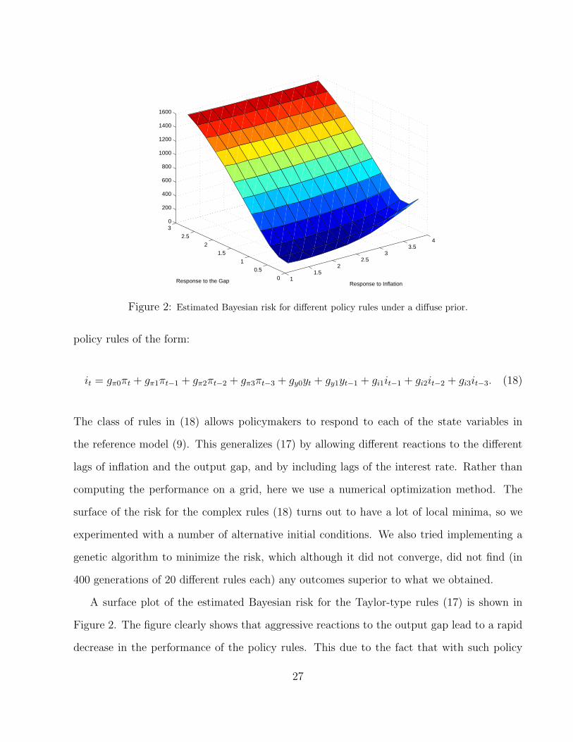
Figure 2: Estimated Bayesian risk for different policy rules under a diffuse prior.
policy rules of the form:
it = gπ0πt + gπ1πt−1 + gπ2πt−2 + gπ3πt−3 + gy0yt + gy1yt−1 + gi1it−1 + gi2it−2 + gi3it−3. (18)
The class of rules in (18) allows policymakers to respond to each of the state variables in
the reference model (9). This generalizes (17) by allowing different reactions to the different
lags of inflation and the output gap, and by including lags of the interest rate. Rather than
computing the performance on a grid, here we use a numerical optimization method. The
surface of the risk for the complex rules (18) turns out to have a lot of local minima, so we
experimented with a number of alternative initial conditions. We also tried implementing a
genetic algorithm to minimize the risk, which although it did not converge, did not find (in
400 generations of 20 different rules each) any outcomes superior to what we obtained.
A surface plot of the estimated Bayesian risk for the Taylor-type rules (17) is shown in
Figure 2. The figure clearly shows that aggressive reactions to the output gap lead to a rapid
decrease in the performance of the policy rules. This due to the fact that with such policy
27

rules, many of the deviations from the RS model turn out to be dynamically unstable, and so
are assigned the maximum risk of 1875. Very aggressive responses to inflation also result in
poor performance, but performance also deteriorates slightly at the low end of the grid.
Table 1 summarizes our results on optimal policy rules in this environment. The first
two lines report the optimal complex rules (18) and Taylor-type rules (17) and the corre-
sponding risk in the present case. The optimal simple rule is on a boundary of our grid at
(gπ, gy) = (1.75, 0.25). (We extended the grid to verify that this is indeed a global minimum.)
This finding is consistent with the Brainard (1967) intuition that the introduction of uncer-
tainty should make policy makers cautious, as the optimal simple rule under no uncertainty
is (2.1, 1.2). Thus uncertainty results in attenuation. Also notice that the performance of the
simple rules is nearly as good as that of the more complex rules. The long run reactions to
inflation and the output gap are nearly the same in the two cases, and the additional flexibility
of the complex rules does not result in much reduction in risk. Further, the optimal complex
rule turns out not to smooth interest rates, as the coefficients on the lagged interest rates
are small and negative at lags two and three. Since we do not assume an interest smoothing
motive, smoothing is not beneficial in this case. However, again the additional feedback on
lagged interest rates is relatively unimportant here in terms of economic performance, as it is
absent in the simple rules.
As we discussed above, in reality policy makers do not mechanically follow policy rules in
practice, whether simple or complex. In particular, policy makers do not commit to a rule
once-and-for-all, but instead would be likely to abandon a rule leading to bad outcomes. While
all modeling of the choice of policy rules involves some abstractions, this suggests that we may
want to re-think our analysis when very bad outcomes result. Furthermore, policymakers likely
know much more than attribute to them. For example, one may a priori believe that most of
the plausible deviations from the RS model will not result in instability if policymakers follow
a rule which closely approximates their observed historical behavior.
28

−0.5 −0.4 −0.3 −0.2 −0.1 0 0.1 0.2 0.3 0.4 0.5−1
−0.8
−0.6
−0.4
−0.2
0
0.2
0.4
0.6
0.8
1
Draws from Posterior for b0 and b
1 under Informative and Uninformative Priors
b0
b 1
Figure 3: Draws from the posterior distribution under a diffuse (orange points) and informative (blackpoints) prior.
To explore this possibility, we compute another sample of MCMC draws assuming in-
formative priors on the coefficients of the polynomials a, b, d, f, and g.10 Recall that these
polynomials correspond to the effects of the macroeconomic variables in the Phillips curve
and IS equation errors. The priors were calibrated so that about 90 percent of the draws from
these prior distributions resulted in dynamic stability under the famous Taylor (1993) rule
of (1.5, 0.5). Such a calibration of the prior distributions changes our posterior distribution
drastically. This is clearly illustrated in Figure 3 which superimposes the MCMC draws from
the posterior distribution of the coefficients b0 and b1 corresponding to the uninformative
and informative priors. The informative priors lead to enormous shrinkage in the posterior
distribution, as the draws are now in a much tighter cloud around zero.
Under the informative priors, Figure 4 shows a surface plot of the inverse of the Bayesian
10Changing the prior for the polynomials c, h, m, and p, which relate to the serial correlation of the drivingshocks, has little effect on the stability of deviations. We choose not to impose informative priors on thepolynomials k and n describing the news content of the real-time data. Doing so, however, does not changeour results much.
29

11.5
22.5
33.5
4
0
0.5
1
1.5
2
2.5
30
0.005
0.01
0.015
0.02
0.025
0.03
0.035
Response to InflationResponse to the Gap
Figure 4: Inverse of the estimated Bayesian risk for different policy rules under an informative prior.
risk for the simple Taylor-type policy rules in our grid. We report the inverted risk because a
few rules in the grid produce extremely large risk, whereas the majority of the rules correspond
to small risk. Such an unbalanced situation distorts the graph so that it is easier interpreted
when inverted. The last two lines of Table 1 above report the optimal complex and simple
rules and their associated risks in this case. For the simple rules, the minimal risk of 29.7
is attained by the rule (2.75, 1.25). Again this does not represent much of a deterioration
from the minimal risk of 29.0 attainable with the more complex rules. Further the long-run
responses to inflation and the output gap are again quite similar in the two cases. Moreover,
Figure 4 shows that the risk is nearly flat over a wide range, resulting in a large region
of rules with comparable risk. For example, the optimal simple rule under no uncertainty
here corresponds to a risk of 33.1, only a 11 percent degradation in performance from the
minimum. Our findings in this case are similar to the results in Rudebusch (2001), who
shows that robustness to many different kinds of uncertainty does not result in a substantial
attenuation of the policy response. In fact, our robust optimal rule with informative priors
30

is more aggressive than the optimal rule in the absence of uncertainty, but the difference in
losses is slight.
Comparing our results under informative and uninformative priors, we see that having
tighter prior beliefs does not greatly improve the expected performance of rules, but it does
lead to more aggressive policy responses. The optimal rules in the informative case are more
aggressive in their responses to both inflation and the output gap than with diffuse priors.
This result holds for both the simple and complex rule specifications. We discussed above
how with a diffuse prior, a number of the deviations from the reference model resulted in
instability when aggressive rules were used. By downweighting the likelihood of instability, the
informative priors rule out many of these outcomes, and so improve the relative performance
of more aggressive rules. However the corresponding minimal risk only falls by roughly 10
percent.
5.2 Minimax Analysis
The Bayesian analysis in the previous section is limited to the parametric model of uncertainty.
We now analyze the robustness of policy rules under the much less restrictive, nonparametric
description of uncertainty we discussed above. However, as we noted there, we do not have
a probability distribution over this nonparametric set. Therefore in this section we use a
minimax approach as in (6), minimizing the worst case loss. For these results, we use the
untruncated loss function:
Lt = π2t + y2
t +1
2i2t .
We estimate a bound on the worst case loss for each policy rule using the algorithm described
in Chapter 6 of Paganini (1996). Unfortunately, there are no theoretical guarantees that the
upper bound on the worst possible loss that we compute is tight. However, our experience
with relatively simple uncertainty descriptions suggests that the gap between the upper bound
31

Optimal Rule Coefficients WorstRule Inflation Out. Gap Lagged Rates CaseType gπ0 gπ1 gπ2 gπ3 gy0 gy1 gi1 gi2 gi3 Loss
Complex 1.28 -0.91 0.66 -0.93 1.57 -1.46 0.49 0.26 0.21 72.3Simple 2.00 1.00 - 79.1
Table 2: The coefficients of the robust optimal minimax rules and corresponding worst-case loss, for boththe complex rules (18) and Taylor-type rules (17).
and the actual worst possible loss is not very large. Moreover, the bound has an appealing
interpretation of the exact worst possible loss under slowly time-varying uncertainty and a
special noise structure (see Paganini (1996)).
We found that nonparametric model uncertainty calibrated using MCMC draws corre-
sponding to an uninformative prior was simply too large to produce interesting results. Since
some of the draws result in instability, the worst case loss was maximal. For such a calibration,
all the simple policy rules on our grid corresponded to dynamic instability in the worst case.
We therefore use the MCMC draws corresponding to the informative prior to calibrate the
uncertainty. Figure 5 shows the inverse of the worst possible losses for the Taylor-type rules
on our grid, and table 2 summarizes the optimal rules in this case. Qualitatively, the graph
is similar to the Bayesian case in Figure 4, with a slightly different peak location. The mini-
mal worst case loss is 79.1 and it is attained by the policy rule (2.0,1.0), which is essentially
indistinguishable on our grid from the optimal rule under no uncertainty. This shows that
the conventional optimal Taylor-type rule, formulated in the absence of model uncertainty,
possesses strong robustness properties. Even though we incorporate an informative prior, lim-
iting perturbations which result in instability, we still allow for a broad range of perturbations
from the reference model. The optimal rule under no uncertainty effectively deals with these
perturbations, and results in good performance under both the reference model (as it was
designed to do) and under the worst case model.
The optimal complex rule also has some interesting features. In contrast to the results in
32

11.5
22.5
33.5
4
0
0.5
1
1.5
2
2.5
30
0.002
0.004
0.006
0.008
0.01
0.012
0.014
Response to InflationResponse to the Gap
Figure 5: Inverse of the worst case losses for different policy rules.
the Bayesian case from Table 1, we now find that some interest rate smoothing is optimal,
as the coefficients on lagged interest rates are larger and all positive. However again, this
interest rate smoothing does not significantly affect losses, as the optimal simple rule (which
clearly lacks smoothing) only leads to a 10 percent degradation in performance relative to the
minimum. Also note that the initial responses to inflation and the output gap (gπ0 and gy0)
are nearly the same in the minimax case as in the Bayesian case with informative priors, but
the rules imply rather different dynamic behavior. In addition to the difference in smoothing,
this is further evidenced by the relatively large negative coefficients on inflation and the output
gap at higher lags in the minimax case. However, these results should be treated with some
caution. In the next section, we discuss why the nonparametric description of uncertainty we
employ here may not be capturing the uncertainty relevant for policy.
33
5.3 Uncertainty at Business Cycle Frequencies
In this section we look at a frequency decomposition of the losses of different policy rules, and
argue that it may be important to restrict attention to rules which deal with uncertainty at
business cycle frequencies. This is a natural consequence of the common view of monetary
policy as a means of smoothing cyclical fluctuations, but not as a fine tuning instrument for
high frequency variation or as an effective way of promoting long-run economic performance.
In general terms, the Rudebusch and Svensson (1999) model coupled with a policy rule for
the interest rate is a way of transferring economic shocks into outcomes of interest, such as
inflation and the output gap. Policymakers arguably should care about the performance of
these target variables at business cycle frequencies. However since the RS model is linear
and time-invariant, this necessarily implies that they must care about offsetting shocks at
business cycle frequencies. In linear time-invariant models, business cycle fluctuations are due
to shocks at business cycle frequencies.
5.3.1 Description and Motivation
We now further describe some reasons why we may want to limit our analysis of uncertainty
to business cycle frequencies. First are the theoretical explanations, reflecting the nature of
our reference model as a model of business cycle fluctuations. The others are more technical,
relating to how our parametric and nonparametric uncertainty descriptions differ in their
treatment of high and low frequency perturbations. We now address each of these in turn.
One of the benefits of minimax analysis is that it provides a simple method of diagnos-
ing possible defects in the model, which also affect the performance of the Bayesian policy
analysis. By inspecting the worst case deviations from the RS model under different policy
rules, we found that for moderately aggressive policy rules the biggest losses result from the
deviations at very low frequencies. More precisely, from (16) the biggest losses are inflicted
34
0 0.2 0.4 0.6 0.8 1 1.20
200
400
600
800
1000
1200
1400
1600
1800
Frequency
Con
trib
utio
n to
the
loss
Transfer of variance across frequencies, rule optimal under no uncertainty
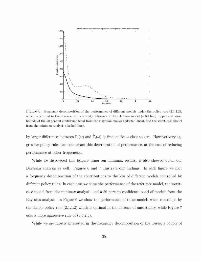
Figure 6: Frequency decomposition of the performance of different models under the policy rule (2.1,1.2),which is optimal in the absence of uncertainty. Shown are the reference model (solid line), upper and lowerbounds of the 50 percent confidence band from the Bayesian analysis (dotted lines), and the worst-case modelfrom the minimax analysis (dashed line).
by larger differences between Γi(ω) and Γi(ω) at frequencies ω close to zero. However very ag-
gressive policy rules can counteract this deterioration of performance, at the cost of reducing
performance at other frequencies.
While we discovered this feature using our minimax results, it also showed up in our
Bayesian analysis as well. Figures 6 and 7 illustrate our findings. In each figure we plot
a frequency decomposition of the contributions to the loss of different models controlled by
different policy rules. In each case we show the performance of the reference model, the worst-
case model from the minimax analysis, and a 50 percent confidence band of models from the
Bayesian analysis. In Figure 6 we show the performance of these models when controlled by
the simple policy rule (2.1,1.2) which is optimal in the absence of uncertainty, while Figure 7
uses a more aggressive rule of (3.5,2.5).
While we are mostly interested in the frequency decomposition of the losses, a couple of
35

0 0.2 0.4 0.6 0.8 1 1.20
200
400
600
800
1000
1200
1400
1600
1800
Frequency
Con
trib
utio
n to
the
loss
Transfer of variance across frequencies, relatively aggressive rule
Figure 7: Frequency decomposition of the performance of different models under a relatively aggressive policyrule (3.5,2.5). Shown are the reference model (solid line), upper and lower bounds of the 50 percent confidenceband from the Bayesian analysis (dotted lines), and the worst-case model from the minimax analysis (dashedline).
36

initial points deserve mention. First, recall that we calibrated our nonparametric description
of uncertainty based on 50 percent confidence regions for each of the different sources of
model error. However in calibrating each channel one-by-one, the resulting joint model has
probability much lower than 50 percent, as the worst-case model from the minimax analysis is
far outside the 50 percent confidence band from the Bayesian analysis. This suggests that in
our minimax analysis we have not accounted for some potentially important joint dependencies
in the model error perturbations. But even with our rough calibration, our minimax analysis
of policy rules turns out to be surprisingly close to the Bayesian analysis. A second important
feature to note is that the reference model often has higher losses than those perturbed models
in the 50 percent confidence band. It turns out, as is described further in Section 5.4 below,
that some of the model error perturbations have a beneficial effect. More precisely, by relaxing
the lag structure of the RS model (but retaining a vertical long-run Phillips curve), many of
the perturbed models are easier to effectively control.
For our purposes, it is interesting to compare the performance of the policy rules at fre-
quencies near zero and at business cycle frequencies. We take the business cycle band to
be those events with periods from 6 to 32 quarters, which corresponds to frequencies from
roughly 0.2 to 1.05. The figures show that there is a clear tradeoff in the performance of
rules at different frequencies. Figure 6 shows that under the benchmark policy rule which is
optimal in the absence of uncertainty, the losses of all models are highest at low frequencies.
As noted above, the performance degradation at low frequencies can be somewhat offset by
choosing a more aggressive policy rule, as Figure 7 illustrates. Now the losses at frequencies
near zero, although still somewhat high, are much lower than before. However this comes at
a clear cost of reducing the performance at business cycle frequencies. Now each model has
another peak in losses between frequencies 0.4 and 0.6, right in the business cycle band. Thus
for less aggressive policy rules, the most damaging perturbations represent deviations in some
of the very long-run properties of the model. This leads the optimal policy rules to become
37

−5 0 5−2
0
2
4a(e0.44i)
−1 0 1−0.5
0
0.5
1b(e0.44i)
−2 0 2−0.5
0
0.5
1d(e0.44i)
−1 0 1−0.5
0
0.5
1f(e0.44i)
−1 0 1−1
−0.5
0
0.5g(e0.44i)
−1 0 1−0.5
0
0.5n(e0.44i)
−2 0 2−2
−1
0
1k(e0.44i)
−5 0 5−3
−2
−1
0
1c(e0.44i)
−2 0 2−1
−0.5
0
0.5
1h(e0.44i)
−2 0 2−1
−0.5
0
0.5
1p(e0.44i)
−2 0 2−1
−0.5
0
0.5m(e0.44i)
Figure 8: MCMC draws (points) and our nonparametric uncertainty bound (circles) at a business cyclefrequency.
more aggressive than they otherwise would be, which worsens their cyclical performance.
However, we feel that changing the low frequency properties of the RS model is pushing the
model too far. We mentioned above that policymakers may be naturally concerned with the
target variables at business cycle frequencies, which would justify downweighting low frequency
perturbations. But in addition, the RS model is designed to explain business cycle frequency
fluctuations and not to describe long-run phenomena. The model is estimated based on de-
meaned quarterly data, and we make no effort to model the means or any possible changes
in the means over time. Additionally, just as the loss function is best viewed as a quadratic
approximation, the reference model is best viewed as a linear approximation to a nonlinear
true model. The linearization is much more appropriate for business cycle fluctuations than
for deviations which may push the model away from its mean for extended periods of time.
A more fully developed model, for example incorporating growth or explicitly modeling time
variation in the data, would be necessary to seriously consider long-run issues.
38

−10 0 10−1
−0.5
0
0.5
1a(e0.01i)
−1 0 1
0
b(e0.01i)
−2 0 2
0
d(e0.01i)
−1 0 1
0
f(e0.01i)
−2 0 2−0.5
0
0.5
g(e0.01i)
−1 0 1
0
n(e0.01i)
−2 0 2
0
k(e0.01i)
−5 0 5−0.5
0
0.5c(e0.01i)
−2 0 2−0.5
0
0.5
h(e0.01i)
−2 0 2−0.5
0
0.5p(e0.01i)
−2 0 2−0.5
0
0.5m(e0.01i)
Figure 9: MCMC draws (points) and our nonparametric uncertainty bound (circles) at a low frequency.
Furthermore, some features of our nonparametric methods increase our measurement of
uncertainty at very low and very high frequencies. Recall that (16) defines the nonparametric
bounds on the transfer functions, which can be viewed as describing a circle in the complex
plane. We calibrate the size of uncertainty by insuring that 50 percent of the MCMC draws
lie within each circle. Thus the circles provide an approximation of a level set of the empirical
distribution of the MCMC draws. This approximation is good if the empirical distribution
is nearly “circular”. However the quality of this approximation decreases substantially if the
empirical distribution of MCMC draws is not circular. For business cycle frequencies, the
approximation seems to be quite good, as Figure 8 shows. The figure plots the MCMC draws
for each Γi(ω), with i = a, . . . , p, associated with the parametric description, along with the
circle containing the possible Γi(ω) for the nonparametric description. The nonparametric
descriptions seem appropriate in this case.
However, if we look at very low frequencies the correspondence breaks down. Recall that
39

our MCMC draws are based on low (second or fourth) order lag polynomials. At very low
(and very high) frequencies the imaginary parts of the transfer functions as in (15) disappear.
For example, p(L) is a second order polynomial, so its transfer function is:
p(ω) = p0 + p1e−iω + p2e
−2iω
= p0 + p1(cos ω − i sin ω) + p2(cos 2ω − i sin 2ω).
Clearly for ω very near zero, both sin ω and sin 2ω will be very near zero, so the imaginary part
will be negligible. Only very high order polynomials have significant imaginary parts at low
frequencies. An illustration of this is shown in Figure 9, which is similar to Figure 8, except
now for a frequency near zero. This clearly shows that in this case, our approximation of the
clouds of MCMC draws by a circle in the complex plane is not accurate. Exactly the same
logic applies for very high frequencies. Thus our calibration of uncertainty is most accurate
for intermediate, business cycle frequencies.
5.3.2 Results
Based on the theoretical and technical considerations outlined above, we therefore extend our
analysis by truncating uncertainty to be zero except at the business cycle frequencies. For the
parametric analysis, we took the mean model from the posterior distribution of the MCMC
draws as the benchmark, and then only included the contributions to the loss coming from
perturbations at business cycle frequencies. For the nonparametric case, in our calibration
we simply set the weights Wa, . . . ,Wp from (16) to be equal to zero for any frequency outside
the range[
2π32
, 2π6
]. We then computed the robust optimal simple rules (17) in the face of
uncertainty at business cycle frequencies.11 For the minimax case, we again looked at rules
11We also computed the optimal complex rules (18) in the minimax case, which gave essentially the sameresults as the simple rules we report here.
40
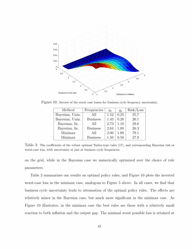
1
1.5
2
2.5
3
3.5
4
0
0.5
1
1.5
2
2.5
3
0
0.01
0.02
0.03
0.04
Response to InflationResponse to the Gap
Figure 10: Inverse of the worst case losses for business cycle frequency uncertainty.
Method Frequencies gπ gy Risk/LossBayesian, Unin. All 1.52 0.25 35.7Bayesian, Unin. Business 1.43 0.26 26.1Bayesian, In. All 2.73 1.18 29.6Bayesian, In. Business 2.64 1.08 26.3
Minimax All 2.00 1.00 79.1Minimax Business 1.50 0.50 27.9
Table 3: The coefficients of the robust optimal Taylor-type rules (17), and corresponding Bayesian risk orworst-case loss, with uncertainty at just at business cycle frequencies.
on the grid, while in the Bayesian case we numerically optimized over the choice of rule
parameters.
Table 3 summarizes our results on optimal policy rules, and Figure 10 plots the inverted
worst-case loss in the minimax case, analogous to Figure 5 above. In all cases, we find that
business cycle uncertainty leads to attenuation of the optimal policy rules. The effects are
relatively minor in the Bayesian case, but much more significant in the minimax case. As
Figure 10 illustrates, in the minimax case the best rules are those with a relatively small
reaction to both inflation and the output gap. The minimal worst possible loss is attained at
41

(1.5,0.5) and equal to 27.9, which is substantially less than the value of 79.1 for uncertainty
at all frequencies. This result is intriguing because the optimal minimax rule coincides with
the Taylor (1993) rule. In the Bayesian case, with both diffuse and informative priors, we find
slight attenuation of the policy response.
The direction and difference in the magnitudes of these effects can be understood by
reference to Figures 6 and 7. In the minimax case, we look for rules that minimize the peak
of the loss function across frequencies. For uncertainty at all frequencies, this requires a rule
more aggressive than the benchmark in Figure 6, which has a huge peak at low frequencies,
but less aggressive than the rule in Figure 7, which lowers the low frequency peak but induces
another one at higher frequencies. But for uncertainty at business cycle frequencies, the figures
suggest that more passive rules have a lower peak over the relevant frequency band. This is
just what we find. The basic idea is the same in the Bayesian case, but instead of minimizing
the peak of the loss function, we now minimize the average loss across frequencies. Thus the
weight put on low frequency perturbations is lower to begin with, so the effect of focusing on
business cycle frequencies is much smaller.
Overall, our results suggest that the aggressiveness of robust policy rules is due to the effects
of fighting off possible movements in inflation and the output gap at very low frequencies.
However if policymakers are more concerned with the performance of policy over the business
cycle horizon, they should instead focus on uncertainty at business cycle frequencies. In this
case, concerns about long-run issues become less important than counter-cyclical stabilization.
This leads policymakers to choose attenuated policy rules.
5.4 Analysis of Distinct Uncertainty Channels
One of the purposes of this paper was to bring together different studies on robustness which
focus on special forms of uncertainty. Therefore, in previous sections, we combined many
42

different sources of uncertainty into one encompassing structure. In this section, we analyze
some of the different components of our uncertainty description taken separately. A goal of
this analysis is to find out which components of the uncertainty have the largest effects on
policy and on losses. This can be useful for researchers working with similar Phillips-curve-
IS-type models, by showing which parts of the specification require the most attention. Our
results here echo the general message we drew from the literature: rules which are robust to
one type of uncertainty may perform poorly when faced with another type.
We now decompose the model uncertainty into its main component parts. These consist
of: (1) uncertainty about the parameters of the reference model and the number of lags
(polynomials a, b, d, f, and g in the error model), (2) uncertainty about the serial correlation
of shocks (c and h), and (3) real-time data uncertainty (k, m, n, and p). We look at the effects
of each of these channels separately. To do this, we simulate different MCMC samples, each
6000 draws long, corresponding to a zero prior on all uncertainty except the chosen uncertainty
channel. Thus, for example, the MCMC sample corresponding to uncertainty about the
parameters and the number of lags is taken under a zero prior on all the parameters of our error
model except the coefficients of a, b, d, f, and g. The prior on the chosen uncertainty channel
is taken to be diffuse. After simulating the MCMC samples, we calibrate the nonparametric
description of uncertainty as outlined in Section 4, and then perform both Bayesian and
minimax analysis of the robustness of Taylor-type policy rules. Instead of analyzing rules on
a grid, we now numerically optimize to compute optimal rules. We also repeat this exercise
to focus on the effects of business cycle uncertainty in the minimax case.
Our results are summarized in Table 4, which provides the coefficients of the optimal
Taylor-type rules for the different uncertainty channels under the different optimization meth-
ods. We also report the corresponding risks or worst-case losses, and for comparison we list
the optimal rule in the absence of uncertainty. The effects of the uncertainty on policy rules
and losses differ significantly in the Bayesian and minimax analysis and across the differ-
43

Bayesian Minimax MinimaxUncertainty All Frequencies All Frequencies Bus. Frequencies
Channel gπ gy Risk gπ gy Loss gπ gy LossNone 2.10 1.20 27.4 2.10 1.20 27.4 2.10 1.20 27.4
Parameters & Lags 1.44 0.55 25.9 - - ∞ - - ∞Noise Correlation 2.14 1.36 32.4 2.09 1.35 45.2 1.98 1.18 34.7Real-Time Data 3.12 1.26 38.7 2.32 1.02 41.5 2.14 0.76 29.8
Table 4: The coefficients of the robust optimal Bayesian and minimax Taylor-type rules and correspondingBayesian risk and worst-case losses. Diffuse priors on specific uncertainty channels, with zero prior on remainingchannels.
ent channels. For uncertainty about the parameters of the model and the lag structure, the
optimal Bayesian response leads to a considerably attenuated policy rule. Interestingly, the
Bayesian risk in this case is also slightly less than the benchmark loss. This happens because
most of the perturbations of the reference model associated with this uncertainty turn out
to be favorable to policymakers, meaning that the perturbed model can be more efficiently
controlled than the reference model. Interest rates need to respond very little to variation
in inflation or the output gap in order to ensure good economic performance. However, even
though most of the perturbations in the parametric case are favorable to policy makers, under
our nonparametric calibration we find that for any policy rule there is a chance of instability.
Thus the maximum loss is infinite, and no minimax policy exists. This is similar to our results
above, and suggests that an informative prior is necessary to rule out instability when dealing
with this uncertainty channel.12
For uncertainty about the serial correlation properties of the shocks, the policy rules are
relatively unaffected in both the Bayesian and minimax cases. Considering uncertainty at all
frequencies, there is a slight increase in the aggressiveness of policy, which again is reduced by
focusing on business cycle frequencies. Overall, the effects of this channel on policy are minor,
with the only significant effect that the worst-case loss at all frequencies increases by about
12We repeated the minimax analysis for this channel with an informative prior, finding the resulting optimalrule (1.69,1.20) with associated worst-case loss of 35.9 at all frequencies. At business cycle frequencies, theoptimal rule is (1.38,0.71) with worst-case loss 22.2.
44
65 percent, but by much less at business cycle frequencies. The perturbations to the serial
correlation of shocks do not really alter the dynamic properties of the transmission of changes
in the interest rate to the other variables. Thus these perturbations have little effect on policy
choice, although they may affect losses through increased volatility. Finally, for real-time data
uncertainty the Bayesian and minimax approaches give somewhat different answers. The
Bayesian analysis finds a relatively aggressive policy rule, especially with respect to inflation,
and this channel has the largest effect on the Bayesian risk. However, the minimax analysis
suggests a smaller increase in the inflation response, and an attenuation of the response to
the output gap. Thus real time data is another important source of uncertainty, although the
policy recommendations depend on whether average or worst case outcomes are optimized.
6 Conclusion
In this paper we analyzed the effects of uncertainty on monetary policy decisions. We con-
sidered three different types of uncertainty: uncertainty about the specification of a reference
model, uncertainty about the serial correlation of noise, and uncertainty about data quality.
We argued that different specifications of uncertainty may have significantly different impli-
cations for monetary policy. Further, uncertainty which enters at different frequencies may
have substantially different effects. It is therefore necessary to model the uncertainty itself
and try to carefully estimate or calibrate the uncertainty model.
We introduced a systematic approach to the formulation of uncertainty relevant for policy
making based on the Model Error Modeling literature. As the name suggests, this approach de-
scribes the uncertainty about an estimated reference model by building models of the model’s
errors. Throughout the paper we focused on a small macroeconometric model of the US econ-
omy proposed and estimated by Rudebusch and Svensson (1999). We formulated models for
the errors of the RS model, focusing on the aspects of uncertainty that are relevant for that
45

model. We then implemented both parametric and nonparametric descriptions of uncertainty
for the model, and used them to design robust monetary policy rules.
Our parametric description of uncertainty assumed that the model errors could be fit
by simple low-order lag polynomials. We estimated these models using Bayesian methods,
obtaining a distribution over the potential alternative models. For use in policy, this led
naturally to Bayesian optimization methods to determine policy rules. The robust rule was
thus the policy rule that minimized Bayesian risk over the distribution of potentially true
models. For the nonparametric description of uncertainty, we did not restrict the order of the
error models, but instead calibrated the size of the uncertainty set in the frequency domain. In
particular, we used our parametric estimates so that at each frequency half of the draws from
the posterior distribution were in our chosen sets. Without having a distribution over this
large (but empirically plausible) class of alternative models, for policy purposes we focused
on minimax optimization methods. In this case, the robust rule was the one that minimized
losses under the worst-case scenario consistent with the uncertainty description.
Without imposing much prior knowledge, we found that the Bayesian optimal policy rules
were attenuated relative to the benchmark case of no uncertainty. However the amount of
uncertainty in our nonparametric specification was too large to produce sensible recommenda-
tions. With uninformative prior beliefs, dynamic instability is a potential outcome for many
policy rules, which suggests a disastrous worst-case scenario. However this result may not be
empirically plausible, particularly for policy which does not strongly deviate from the past.
Therefore we then imposed stronger prior beliefs to downweight the likelihood of instability.
We found that the resulting Bayesian optimal policy rule was more aggressive than in the
absence of uncertainty, while the minimax rule was quite close to this no-uncertainty bench-
mark. However all of these rules are still relatively aggressive, especially in comparison to
directly estimated policy rules.
Our analysis also showed that very low frequency perturbations often have the most impact
46

on policy. There is a clear relationship between the aggressiveness of policy rules and the
performance of rules at different frequencies. More aggressive rules perform better at low
frequencies, at the cost of deteriorating performance at business cycle frequencies. Since our
baseline model is essentially a model of short-run fluctuations, we felt that it was extreme
to ask it to accommodate very low frequency perturbations. Therefore we recalculated our
results by restricting attention to business cycle frequencies. In these cases we found that
instead of reacting aggressively, our policy rules were more attenuated than in the absence of
uncertainty. Under some specifications, our results were quite close to the policy rules that
have been directly estimated. We also analyzed separately the effects uncertainty of each of
the different channels. We found that uncertainty about the parameters and lag structure of
the model is probably the most important channel, but that real-time data uncertainty can
also be important for optimal policy rules.
Many important issues are left for future research. For example, in this paper we left open
the question of how to choose a reference model. Additionally, the baseline model that we
used was intentionally simple, and completely backward looking. Much more could be done to
extend both the baseline model that we analyze and therefore the methods we use, for example
to consider forward-looking behavior or unrestricted optimal policy rules. This paper is only
a first step in the analysis, but even by focusing on a simple case we find some interesting
results. More work remains to be done to accurately measure the uncertainty relevant for
policy. This requires even more careful modeling of model uncertainty.
References
Ball, Laurence (1999). “Policy Rules for Open Economies.” In Monetary Policy Rules, edited
by J. Taylor. Chicago: University of Chicago Press for the NBER.
Blinder, Alan (1997). “Distinguished Lecture on Economics in Government: What Central
47

Bankers Could Learn from Academics - and Vice Versa.” Journal of Economic Perspectives ,
11, pp. 3–19.
Brainard, William (1967). “Uncertainty and the Effectiveness of Policy.” American Eco-
nomic Review , 57, pp. 411–425.
Chib, Siddhartha and Edward Greenberg (1994). “Bayes Inference in Regression Models
with ARMA(p,q) Errors.” Journal of Econometrics , 64, pp. 183–206.
Craine, Roger (1979). “Optimal Monetary Policy with Uncertainty.” Journal of Economic
Dynamics and Control , 1, pp. 59–83.
Hansen, Lars Peter and Thomas J. Sargent (2002). Robust Control and Model Uncertainty
in Macroeconomics. Mimeo. University of Chicago.
Levin, Andrew, Volker Wieland, and John C. Williams (1999). “Robustness of Simple
Monetary Policy Rules under Model Uncertainty.” In Monetary Policy Rules, edited by
J. Taylor. Chicago: University of Chicago Press for the NBER.
Ljung, Lennart (1999). “Model Validation and Model Error Modeling.”. Control and Com-
muncations Group Technical Report LiTH-ISY-R-2125, Linkoping University.
Mankiw, N. Gregory and Matthew D. Shapiro (1986). “News or Noise: An Analysis of GNP
Revisions.” Survey of Current Business , 66, pp. 20–25.
Mas-Colell, Andreu, Michael D. Whinston, and Jerry R. Green (1995). Microeconomic
Theory. Oxford University Press.
McCallum, Bennett T. (1988). “Robustness Properties of a Rule for Monetary Policy.”
Carnegie-Rochester Conference Series on Public Policy , 29, pp. 175–203.
Onatski, Alexei and James H. Stock (2002). “Robust Monetary Policy under Model Uncer-
tainty in a Small Model of the US Economy.” Macroeconomic Dynamics , 6, pp. 85–110.
48

Orphanides, Athanasios (2001). “Monetary Policy Rules Based on Real-Time Data.” Amer-
ican Economic Review , 91, pp. 964–985.
Paganini, Fernando (1996). Sets and Constraints in the Analysis of Uncertain Systems.
Unpublished Ph.D. dissertation, California Institute of Technology.
Priestley, Maurice B. (1981). Spectral Analysis and Time Series. Academic Press.
Rudebusch, Glenn D. (2001). “Is the Fed Too Timid? Monetary Policy in an Uncertain
World.” Review of Economics and Statistics , 83, pp. 203–217.
Rudebusch, Glenn D. and Lars E. O. Svensson (1999). “Policy Rules for Inflation Target-
ing.” In Monetary Policy Rules, edited by J. Taylor. Chicago: University of Chicago Press
for the NBER.
Sargent, Thomas J. (1999). “Discussion of ‘Policy Rules for Open Economies,’ by L. Ball.”
In Monetary Policy Rules, edited by J. Taylor. Chicago: University of Chicago Press for
the NBER.
Soderstrom, Ulf (2002). “Monetary Policy with Uncertain Parameters.” Scandinavian Jour-
nal of Economics , 104, pp. 125–145.
Swanson, Eric T. (2000). “On Signal Extraction and Non-Certainty-Equivalence in Optimal
Monetary Policy Rules.”. Mimeo, Federal Reserve Board.
Taylor, John B. (1993). “Discretion versus Policy Rules in Practice.” Carnegie-Rochester
Conference Series on Public Policy , 39, pp. 195–214.
Woodford, Michael D. (2002). Interest and Prices: Foundations of a Theory of Monetary
Policy. Princeton: Princeton University Press. Forthcoming.
49
Recommended