
Modular FormsSpring 2011 Notes (and beyond)
Kimball Martin
June 26, 2019

Preface
The first part of these notes are based on a graduate course on modular forms I gave inSpring 2011 at the University of Oklahoma. The second part of these notes, still in progress,consists of additional topics I did not cover in the course, but which I might imagine coveringin a second semester.
Preface to first part
In the first part, I have tried to give an introduction to modular forms with a view towardsclassical applications, such as quadratic forms and functions on Riemann surfaces, as opposedto “modern applications” (in the sense of requiring a more modern perspective) such asFermat’s last theorem and the congruent number problem.
At the same time, I have tried to give a suitable introduction to lead into a one-semestercourse on automorphic forms and representations (in Fall 2011), which meant a slightlydifferent balance of material than in a course wholly focusing on classical modular forms.
I also tried to keep the prerequisites as minimal as possible while attempting to meetboth of these goals.
For those considering using these notes: you can get an idea of the contents by lookingat the table of contents and skimming through, so I won’t elaborate on them here, but justsay the following points, which distinguish the presentation from some other treatments:
(1) My general philosophy is to find a balance between simplicity and completeness,focusing on what I think is important to understanding the ideas and being able to seeapplications, rather than favoring either generalities or minutia—of course my preferredbalance may be different than yours. (2) I try to give geometric motivation to the definitionof modular forms. (3) I primarily focus on modular forms on Γ0(N) and do not evenintroduce modular forms with character (nebentypus). (4) I try to be fairly explicit witharithmetic (e.g., working out Fourier expansions of Eisenstein series with level and explicitformulas for representation numbers of quadratic forms), though I don’t go overboard (oreven as far along the board as I wanted). (5) I finish the first part with a brief treatment ofL-functions, which I will hopefully expand on later, possibly in the second part.
A warning and an apology are in order.The warning: several of the sections were written in a rush, and may have some (hopefully
not serious) errors. Please email me if you find any mistakes, so I can correct them.The apology: due to weather and travel, we missed many lectures, and as a result there
are many things missing that I would have liked to include, such as Siegel modular forms
1

2
and the structure of modular functions. Further, there are many details that I would like tohave included which I had not the time for. In addition, I realize now I could have done abetter job filling in some prerequisite material. Upon teaching this course again, or possiblyearlier if I am inspired, I plan to revise these notes. (I have made minor revisions to thefirst part, but no serious ones since.) If you have any comments or suggestions, I would behappy to hear them.
I would like to thank my students, for asking many questions and pointing out manymistakes in early versions of these notes, in particular: Kumar Balasubramanian, Jeff Breed-ing, James Broda, Shayna Grove, Catherine Hall, Daniel McLaury and Salam Turki. I amalso grateful to Victor Manuel Aricheta and Roberto Miatello for pointing out additionalerrors.
Preface to second part
Recently (2014–2015) I started thinking again to write up notes on some additional topics Idid not cover in the one-semester modular forms course, e.g.: newforms, half-integral weightforms (though I didn’t even do odd weight in the first part!), quaternionic modular forms,Eichler–Shimura theory, modularity of elliptic curves, Hilbert modular forms, Siegel modularforms. (Though, perhaps surprising to some, I still have no desire to cover modular formswith character—there’s no accounting for taste, you know). I was contemplating teaching asecond semester course in modular forms in Spring 2016, but there was no modular formscourse in Fall 2015, and I instead decided to teach a course on (Quaternion) Algebras inNumber Theory. The notes for that course should eventually discuss quaternionic modularforms and the Jacquet–Langlands correspondence, at least in simple situations.
Still, I made some progress in 2015–2016 by adding an unpolished chapter on newformsto begin the second part, which is a slow work in progress (currently in progress: a chapteron Hilbert modular forms). While I don’t plan on doing a comprehensive treatment of thetopics in the second part, or necessarily give complete proofs, I hope to give a more-or-lessworking introduction to these topics.

Contents
Preface 1
I The basic course 5
1 Introduction 6
2 Elliptic functions 112.1 Complex analysis review: Holomorphy . . . . . . . . . . . . . . . . . . . . . . 112.2 Complex analysis review II: Zeroes and poles . . . . . . . . . . . . . . . . . . 142.3 Periodic functions . . . . . . . . . . . . . . . . . . . . . . . . . . . . . . . . . . 162.4 Doubly periodic functions . . . . . . . . . . . . . . . . . . . . . . . . . . . . . 202.5 Elliptic functions to elliptic curves . . . . . . . . . . . . . . . . . . . . . . . . 23
3 The Poincaré upper half-plane 263.1 The hyperbolic plane . . . . . . . . . . . . . . . . . . . . . . . . . . . . . . . . 263.2 Fractional linear transformations . . . . . . . . . . . . . . . . . . . . . . . . . 283.3 The modular group . . . . . . . . . . . . . . . . . . . . . . . . . . . . . . . . . 313.4 Congruence subgroups . . . . . . . . . . . . . . . . . . . . . . . . . . . . . . . 353.5 Cusps and elliptic points . . . . . . . . . . . . . . . . . . . . . . . . . . . . . . 39
4 Modular Forms 444.1 Modular curves and functions . . . . . . . . . . . . . . . . . . . . . . . . . . . 444.2 Eisenstein series . . . . . . . . . . . . . . . . . . . . . . . . . . . . . . . . . . . 494.3 Modular forms . . . . . . . . . . . . . . . . . . . . . . . . . . . . . . . . . . . 614.4 Theta series . . . . . . . . . . . . . . . . . . . . . . . . . . . . . . . . . . . . . 664.5 η and ∆ . . . . . . . . . . . . . . . . . . . . . . . . . . . . . . . . . . . . . . . 72
5 Dimensions of spaces of modular forms 785.1 Dimensions for full level . . . . . . . . . . . . . . . . . . . . . . . . . . . . . . 785.2 Finite dimensionality for congruence subgroups . . . . . . . . . . . . . . . . . 87Appendix: Dimension Tables . . . . . . . . . . . . . . . . . . . . . . . . . . . . . . 92
6 Hecke operators 956.1 Hecke operators for Γ0(N) . . . . . . . . . . . . . . . . . . . . . . . . . . . . . 966.2 Petersson inner product . . . . . . . . . . . . . . . . . . . . . . . . . . . . . . 106
3

CONTENTS 4
7 L-functions 1137.1 Degree 1 L-functions . . . . . . . . . . . . . . . . . . . . . . . . . . . . . . . . 113
7.1.1 The Riemann zeta function . . . . . . . . . . . . . . . . . . . . . . . . 1137.1.2 Dirichlet L-functions . . . . . . . . . . . . . . . . . . . . . . . . . . . . 115
7.2 The philosophy of L-functions . . . . . . . . . . . . . . . . . . . . . . . . . . . 1177.3 L-functions for modular forms . . . . . . . . . . . . . . . . . . . . . . . . . . . 119
II Selected topics 124
8 Newforms and oldforms 1268.1 Hecke operators via double cosets . . . . . . . . . . . . . . . . . . . . . . . . . 1278.2 Hecke operators on Eisenstein series . . . . . . . . . . . . . . . . . . . . . . . 1308.3 Atkin–Lehner operators . . . . . . . . . . . . . . . . . . . . . . . . . . . . . . 1348.4 New and old forms . . . . . . . . . . . . . . . . . . . . . . . . . . . . . . . . . 135
9 Hilbert modular forms 1429.1 Basic definitions and results . . . . . . . . . . . . . . . . . . . . . . . . . . . . 143
References 146
Index 149
Part I
The basic course
5

Chapter 1
Introduction
There are many starting points for the theory of modular forms. They are a fundamentaltopic lying at the intersection of number theory, harmonic analysis and Riemann surfacetheory. Even from a number theory point of view, there are several ways to motivate thetheory of modular forms. One is via the connection with elliptic curves, made famousthrough Wiles’ solution to Fermat’s Last Theorem. This connection has many amazingimplications in number theory, but we will emphasize the role of modular forms in thetheory of quadratic forms.
Let Q be a quadratic form of rank k over Z. This means Q is a homogeneous polynomialof degree 2 over Z in k variables with a certain nondegeneracy condition. For example, Qmight be a diagonal form
Q(x1, . . . , xk) = a1x21 + a2x
22 + · · ·+ akx
2k (1.0.1)
where each ai 6= 0; or it may be something like Q(x, y) = x2 + 2xy + 3y2. Regardless, thefundamental question about Q is
Question 1.1. What numbers does Q represent? In other words, for which n does
Q(x1, . . . , xk) = n
have a solution in Z?
There is a more quantitative version of this question as follows.
Question 1.2. Let rQ(n) denote the number of solutions (in Z) to
Q(x1, . . . , xk) = n.
Determine rQ(n).
Note that an answer to Question 1.2 provides an answer to Question 1.1, since Question1.1 is simply asking, when is rQ(n) > 0? (Sometimes rQ(n) is infinite, and instead onecounts solutions up to some equivalence, but we will not go into this here.)
Let us consider the specific examples of forms
Qk(x1, . . . , xk) = x21 + x2
2 + · · ·+ x2k,
6

CHAPTER 1. INTRODUCTION 7
and write rQk(n) simply as rk(n). So Question 1.1 is simply the classical question, whatnumbers are sums of k squares? Lagrange proved that every positive integer can be writtenas a sum of four squares (and therefore ≥ 4 squares by just taking xi = 0 for i > 4). Thecases of sums of two squares and sums of three squares were answered by Fermat and Gauss.So a complete answer to Question 1.1 for the forms Qk has been known since the time ofGauss (who did fundamental work on quadratic forms), but the answer for k > 4 is not sointeresting, as it is trivially encoded in the answer for k = 4.
Hence at least for these forms, we see the question of determining rk(n) is much more in-teresting. Furthermore, Question 1.1 is typically much more difficult for arbitrary quadraticforms Q than it is for Qk, and a general method for answering Question 1.2 will provide usa way to answer Question 1.1.
Now let us briefly explain how one might try to find a formula for rk(n). Jacobi consideredthe theta function
ϑ(z) =∞∑
n=−∞qn
2, q = e2πiz. (1.0.2)
This function is well defined for z ∈ H = x+ iy : x, y ∈ R, y > 0. Then
ϑ2(z) =
( ∞∑`=−∞
q`2
)( ∞∑m=−∞
qm2
)=∑`,m
q`2+m2
=∑n≥0
r2(n)qn.
Similarly,ϑk(z) =
∑n≥0
rk(n)qn. (1.0.3)
(More generally, if Q is the diagonal form in (1.0.1), then we formally have∏ki=1 ϑ(aiz) =∑
rQ(n)qn.) It is not too difficult to see that ϑk satisfies the identities
ϑk(z + 1) = ϑk(z), ϑk(−1
4z
)=
(2z
i
) k2
ϑk(z). (1.0.4)
Indeed, the first identity is obvious because q is invariant under z 7→ z + 1.The space of (holomorphic) functions on H satisfying the transformation properties is
(1.0.4) is defined to be the space of modular forms Mk/2(4) of weight k/2 and level 4. Thetheory of modular forms will tell us that Mk/2(4) is a finite-dimensional vector space.
For example, when k = 4, M2(4) is a 2-dimensional vector space, and one can find abasis in terms of Eisenstein series. Specifically, consider the Eisenstein series
G(z) = − 1
24+∞∑n=1
σ(n)qn,
where σ(n) is the divisor function σ(n) =∑
d|n d. Then a basis of M2(4) is
f(z) = G(z)− 2G(2z), g(z) = G(2z)− 2G(4z).
Hence ϑ4(z) is a linear combination of f(z) and g(z). How do we determine what combina-tion? Simply compare the first two coefficients of qn in af(z) + bg(z) with ϑ4(z), and onesees that
ϑ4(z) = 8f(z) + 16g(z).

CHAPTER 1. INTRODUCTION 8
Expanding this out, one sees that
ϑ4(z) =∑n≥0
r4(n)qn = 1 + 8∑n≥1
σ(n)qn − 32∑n≥1
σ(n)q4n. (1.0.5)
Consequently
r4(n) =
8σ(n) 4 - n8σ(n)− 32σ(n/4) 4|n.
If one wishes, one can write this as a single formula
r4(n) = 8 (2 + (−1)n)∑d|n,2-d
d. (1.0.6)
In particular, it is obvious that r4(n) > 0 for all n, in other words, we have Lagrange’stheorem that every positive integer is a sum of four (not necessarily nonzero) integer squares.Furthermore, we have a simple formula for the number of representations of n as a sum offour squares, in terms of the divisors of n.
In this course, we will develop the theory of modular forms, and use this to derive variousformulas of the above type. Along the way, we will give some other applications of modularforms. We will also introduce the theory of L-functions, which are an important tool inthe theory of modular forms, and are fundamental in the connection with elliptic curves.Time permitting, we will introduce generalizations of modular forms, such as Siegel modularforms and automorphic forms.
As much as possible, we will try to keep the prerequisites to a minimum. Certainly,working knowledge of linear algebra is expected, as well as some familiarity with groups andrings. Familiarity with elementary number theory is helpful but not necessary (modulararithmetic will be used, as well as some standard notation from elementary number theory).We may at times discuss some aspects of basic algebraic number theory, but these discussionsshould be sufficiently limited to not greatly affect the flow of the text if ignored.
Particularly in the beginning, we will be discussing geometric ideas, as this providesmotivation for studying modular forms (why study functions on the upper-half plane Hsatisfying seeming strange transformation laws as in (1.0.4)?). Here, familiarity with suchthings as Riemann surfaces, isometry groups and universal covers will be helpful, but wewill develop the needed tools as we go. Some basic notions of point-set topology (open sets,continuity, etc.) will be assumed.
Perhaps most helpful will be a solid course on complex analysis (fractional linear trans-formations, holomorphy, meromorphy, Cauchy’s integral formula, etc.) and familiarity ofFourier analysis. For those lacking (or forgetting) this analysis background, I will recall thenecessary facts as we go, but the reader should refer to texts on complex analysis or Fourieranalysis for further details and proofs.
There are a variety (but not a plethora) of exercises intertwined with the text. Most ofthem are not too difficult, and I encourage you to think about all of them, whether or notyou decide it’s worth your while to work out the details. I have starred certain exerciseswhich I consider particularly important. You may find a larger selection of exercises fromthe references listed below.
CHAPTER 1. INTRODUCTION 9
There are many good references for the basic theory of modular forms. Unfortunately,none of them do exactly what we want, which is why I am writing my own notes. Alsounfortunately, the terminology and notation among the various texts is not standarized. Onthe other hand, they are better at what they do than my notes (and likely with fewer errors),so you are encouraged to refer to them throughout the course.
• [Ser73] Serre, J.P. A course in arithmetic. A classic streamlined introduction to mod-ular forms of level 1. Many of the details you need to work out for yourself.
• [Kob93] Koblitz, Neal. Introduction to elliptic curves and modular forms. A solid intro-duction to modular forms of both integral and half-integral weight (or arbitrary level),if slightly dense. The goal is to present them in connection with elliptic curves andshow how they are used in Tunnell’s solution, assuming the weak Birch–Swinnerton-Dyer conjecture, of the ancient congruent number problem.
• [Kil08] Kilford, L.J.P. Modular forms: a classical and computational introduction. Anew book, and it seems like a good introduction to modular forms. Has errata online.The one thing lacking for our course is that it does not cover L-functions.
• [Zag08] Zagier, Don. Elliptic modular forms and their applications, in “The 1-2-3 ofmodular forms.” A beautiful overview of modular forms (primarly level 1) and theirapplications. Available online.
• [Lan95] Lang, Serge. Introduction to modular forms. It’s Serge Lang. Covers someadvanced topics.
• [Apo90] Apostol, Tom. Modular functions and Dirichlet series in number theory. Anice classical analytic approach to modular forms.
• [Mil] Milne, J.S. Modular functions and modular forms. Online course notes. Thistreatment, somewhat like [DS05] or [CSS97], has a more geometric focus (e.g., modularcurves).
• [DS05] Diamond, Fred and Shurman, Jerry. A first course in modular forms. An ex-cellent book, perhaps requiring more geometric background than others, focusing onthe connections of modular forms, elliptic curves, modular curves and Galois repre-sentations. Available online.
• [Iwa97] Iwaniec, Henryk. Topics in classical automorphic forms. An excellent andfairly elementary analytic approach using classical automorphic forms. Many interest-ing applications are presented.
• [Miy06] Miyake, Toshitsune. Modular forms. A fairly advanced presentation of thetheory of modular forms, starting with automorphic forms on adeles. Contains usefulmaterial not easily found in many texts. Available online.
• [Bum97] Bump, Daniel. Automorphic forms and representations. A thorough (at leastas much as possible in 550 pp.) text on automorphic forms and representations onGL(n). The first quarter of the book treats classical modular forms.
CHAPTER 1. INTRODUCTION 10
• [Ste07] Stein, William. Modular forms: a computational approach. Perhaps a usefulreference for those wanting to do computations with modular forms.
• [CSS97] Cornell, Silverman and Stevens (ed.s). Modular forms and Fermat’s last the-orem. A nice collection of articles giving an overview of the theory of elliptic curves,modular curves, modular forms and Galois representations, and how they are used toprove Fermat’s last theorem.
Chapter 2
Elliptic functions
Before we introduce modular forms, which, as explained in the introduction, are functionson the upper half-plane, or the hyperbolic plane, satisfying certain transformation laws, itmay be helpful to get a basic understanding of elliptic functions, which are functions on Csatisfying certain simpler transformation laws. That is our goal for this chapter.
Elliptic functions are a classical topic in complex analysis, and their theory can be foundin several books on the subject, such as [Ahl78], [Lan99], [FB09] (available online) or [Sta09](available online), as well as many texts on elliptic curves and modular forms (e.g., [Kob93],[Iwa97]). In fact, the complex analysis books [FB09] and [Sta09] discuss modular forms.Since elliptic functions are not a focus for this course, but rather a tool for motivation ofthe theory of modular forms, we will not strive for rigorous proofs, but merely conceptualunderstanding. Put another way, this chapter is a sort of summary of the pre-history ofmodular forms.
We will explain later how the theory of elliptic functions is essentially a “Euclideanversion” of the theory of modular forms, and in fact modular forms first arose from thestudy of elliptic functions.
2.1 Complex analysis review: Holomorphy
First let us review some basic facts from the theory of functions of one complex variable.Let C denote the complex plane. Throughout these notes, z will denote a complex
number, and unless stated otherwise, x and y will denote the real and imaginary parts,x = Re(z) and y = Im(z), of z. I.e., z = x+ iy where x, y ∈ R.
Let f : C → C. As vector spaces, we clearly have C ' R2 via the linear isomorphismz 7→ (x, y), hence we may also view f as a function from R2 to R2. In fact, C and R2
are isomorphic as topological spaces, so the notion of continuity is the same whether weregard f as a function on C or R2. The conceptual difference between functions on C andR2 arises when we study the notion of differentiablilty, and the difference arises because onecan multiply complex numbers, but not (naturally) elements of R2.
Specifically, look at the condition
f ′(z) = limh→0
f(z + h)− f(z)
h. (2.1.1)
11

CHAPTER 2. ELLIPTIC FUNCTIONS 12
If we want to think of f as truly a function of C, this means we should be taking h ∈ Cin the above limit. In other words, unlike in the real case where h can only approach 0from the left or right, here h can approach 0 along any line or path to the origin in C. Inparticular, (2.1.1) should be true for h ∈ R and h = ik ∈ iR. Note, restricting to h ∈ Rin the limit above amounts to differentiating with respect to x, and restricting to h ∈ iRamounts to differentiating with respect to y.
We can write f(z) uniquely as f(z) = u(z) + iv(z) where u : C→ R and v : C→ R, i.e.,u = Re(f) and v = Im(f). We also write u(z) = u(x, y) and v(z) = v(x, y). Then condition(2.1.1) taking h ∈ R means
f ′(z) = limh→0
f(x+ h+ iy)− f(x+ iy)
h
= limh→0
u(x+ h, y) + iv(x+ h, y)− u(x, y)− iv(x, y)
h
= limh→0
u(x+ h, y)− u(x, y)
h+ i lim
h→0
v(x+ h, y)− v(x, y)
h
=∂u
∂x+ i
∂v
∂x.
Similarly, taking h = ik ∈ iR in (2.1.1) means
f ′(z) = limk→0
f(x+ i(y + k))− f(x+ iy)
ik
= limk→0
u(x, y + k) + iv(x, y + k)− u(x, y)− iv(x, y)
ik
= limk→0
u(x, y + k)− u(x, y)
ik+ i lim
k→0
v(x+ k, y)− v(x, y)
ik
=1
i
(∂u
∂y+ i
∂v
∂y
)=∂v
∂y− i∂u
∂y.
Comparing the real and imaginary parts of these 2 expressions for f ′(z) gives the Cauchy–Riemann equations
∂u
∂x=∂v
∂y,
∂v
∂x= −∂u
∂y. (2.1.2)
Definition 2.1.1. Let U ⊆ C be an open set. We say f : U → C is (complex) differ-entiable, or holomorphic, at z if the limit limh→0
f(z+h)−f(z)h exists (for h ∈ C). In this
case, the derivative f ′(z) is defined to be the value of this limit.We say f is holomorphic on U if f is holomorphic at each z ∈ U . If f is holomorphic
on all of C, we say f is entire.
As we saw above, being holomorphic on an open set U means that the Cauchy–Riemannequations will hold (and the partial derivatives will be continuous). (This is in fact if and onlyif.) Contrast this to differentiable functions on R2: if one knows the partial derivatives existand are continuous on an open set in R2, the function is (real) differentiable there. TheCauchy–Riemann equations give a much stronger condition for a function to be complexdifferentiable.
CHAPTER 2. ELLIPTIC FUNCTIONS 13
The biggest consequence of the Cauchy–Riemann equations is that if f is holomorphic onU , so is f ′. Hence being differentiable once means being infinitely differentiable. This featuremakes complex analysis much nicer than real analysis. In particular, any differentiablefunction on U has a Taylor series expansion around any z0 ∈ U :
f(z) = f(z0) + f(z − z0) +f ′′(z0)
2!(z − z0)2 +
f ′′′(z0)
3!(z − z0)3 + · · · .
Recall that any power series∑
n≥0 an(z − z0)n has a radius of convergence R ∈ [0,∞]such that the series converges absolutely for |z − z0| < R and diverges for |z − z0| > R.
Definition 2.1.2. Let U be an open set in C and f : U → C. We say f is analytic atz0 ∈ U if, for some R > 0, we can write
f(z) =∑n≥0
an(z − z0)n, |z − z0| < R.
We say f is analytic on U if f is analytic at each z0 ∈ U .
Note if we can write f(z) as a power series∑
n≥0 an(z − z0)n about z0, and this serieshas radius of convergence R, then f is analytic on the open disc |z − z0| < R.
One of the main theorems of complex analysis is
Theorem 2.1.3. Let U be an open set of C and f : U → C. The following are equivalent.(i) f is holomorphic on U ;(ii) f is infinitely differentiable on U ;(iii) f if analytic on U ; and(iv) If u = Re(f) and v = Im(f), then the partial derivatives of u and v with respect to
x, y exist, are continuous, and satisfy the Cauchy–Riemann equations.
From the definition, it is clear differentiation over C satisfies the usual differentiationrules of calculus (sum, product, quotient and chain rules; as well as the power rule andderivative formulas for trigonometric and exponential functions).
For n ∈ Z, the power functions f(z) = zn are well defined and entire for n ≥ 0, andholomorphic on the punctured plane C− 0 for n < 0.
Exercise 2.1.4. Consider f(z) = 1z . Show f satisfies the Cauchy–Riemann equations.
Deduce that it is analytic on its domain, but there is no single power series expansion validfor all z ∈ C− 0.
One can define ez, sin(z) and cos(z) by the usual Maclaurin series expansions
ez =∞∑n=0
zn
n!,
sin(z) =
∞∑n=0
(−1)nz2n+1
(2n+ 1)!,

CHAPTER 2. ELLIPTIC FUNCTIONS 14
and
cos(z) =∞∑n=0
(−1)nz2n
(2n)!.
These series have radius of convergence ∞, and hence define entire functions.On the other hand, the logarithm cannot be extended to an entire function. The best
one can do is make it well defined on the complex plane minus a ray from the origin. Thisinvolves choosing a “branch cut.” Unless otherwise specified, we will chose our branch cutsso that the complex logarithm is holomorphic function on C− R≤0
Power functions for non-integral exponents can be defined in terms of the logarithm.Specifically, one can formally define za = ea log z. This will be holomorphic when the loga-rithm is, which will typically be C− R≤0 for us.
Some basic facts about analytic functions are recorded in the following.
Theorem 2.1.5. Let z0 ∈ C and f be defined on a neighborhood of z0. Suppose f is analyticat z0. Then f is analytic in a neighborhood U of z0. Furthermore, we have the following.
(a) If f ′ is nonzero on U , then f is conformal, i.e., f preserves angles.(b) If f ′(z0) 6= 0, then f is locally invertible at z0, i.e., there exist a function g which is
analytic near f(z0) such that g f = id near z0.(c) Let S be a subset of U containing an accumulation point. If g : U → C is analytic
and f(z) = g(z) for z ∈ S, then f(z) = g(z) for all z ∈ U .
The first part of the theorem follows from the fact we already remarked after Definition2.1.2. Part (a) says that analytic function preserve a lot of geometry. Even though theydo not in general preserve distance, this property of preserving angles forces certain rigidbehavior of analytic functions. For instance, conformality implies that there is no analyticfunction mapping an open disc to an open square. Another example of this rigid behaviouris Liouville’s function, which we will state later, but geometrically says that no analyticfunction can map the complex plane to any bounded region. Part (c) also describes arigidity feature: an analytic function is determined by its values on merely a countable setof points (which contains an accumulation point).
2.2 Complex analysis review II: Zeroes and poles
The most basic analytic information about an analytic function is the location of its zeroesand poles. Let’s start off discussing zeroes, although there’s not much to say at the moment.
Definition 2.2.1. Let f be analytic at z0 such that f(z0) = 0. We say f has a zero oforder m at z0 if limz→z0
f(z)(z−z0)m exists and is nonzero, or, equivalently, if the power series
expansion of f at z0 has the form
f(z) =
∞∑n=m
an(z − z0)n
with am 6= 0.
CHAPTER 2. ELLIPTIC FUNCTIONS 15
Note that zeroes of a nonconstant analytic function must be isolated, i.e., they form adiscrete set. To see this, suppose f is analytic on U , and let S be the set of zeroes of f . Iff is nonconstant and S has an accumulation point, then Theorem 2.1.5(c) implies f ≡ 0 onU . In particular, in any bounded region, an nonzero analytic function has a finite numberof zeroes.
Definition 2.2.2. Let U be a neighborhood of z0 and f be a nonconstant analytic functionon U − z0. We say f has a pole of order m at z0 if 1
f(z) has a zero of order m atz0, or, equivalently, limz→z0(z − z0)mf(z) exists and is nonzero. In this case, we writef(z) = limz→z0 f(z) =∞.
If one wants to be a little more formal about assigning a value of ∞ to f , consider theRiemann sphere C = P1(C) = C ∪ ∞. (Here the open sets of C are generated by theopen sets of C together with the balls about infinity, z : |z| > ε∪∞, for ε ∈ R≥0. HenceC is topologically a sphere.) Even though there are infinitely many “real directions” to gooff to infinity in C (meaning picturing C as R2), we think of them all leading to the samepoint, ∞, on C.
In fact, one can push this idea further. If f : C → C, one can define a value for f(∞)and think of f : C→ C, and one can talk about analytic maps from the Riemann sphere toitself.
We need a term for analytic functions with poles (since functions are not called analytic,or holomorphic, at their poles).
Definition 2.2.3. Let U ⊆ C be an open set and f : U → C. Let S = f−1(∞) ⊆ U be theset of poles of f in U . If S is discrete and f is analytic on U−S, we say f is meromorphicon U .
In particular, if f and g are holomorphic functions on U and g 6≡ 0, then f/g is meromor-phic on U . This follows from the fact that f/g is differentiable outside of the set of zeroesof S, which we remarked above is discrete. Hence all rational functions are meromorphicon C. Specifically, if f and g are nonzero polynomials, then the number of zeroes (countingmultiplicity, i.e., summing up the orders of zeroes) of f/g is deg(f) and the number of poles(again counting with multiplicity) is deg(g).
Just like a holomorphic function has a power series expansion about any point in itsdomain, a meromorphic function has a Laurent series expansion around any point in itsdomain.
Suppose f : U → C is meromorphic, and let z0 ∈ C. If f(z0) 6= ∞, then we just havea usual power series expansion f(z) =
∑∞n=0 an(z − z0)n valid near z0. Suppose instead f
has a pole of order m at z0. Then (z− z0)mf(z) is holomorphic near z0, so we have a powerseries expansion
(z − z0)mf(z) =
∞∑n=0
an(z − z0)n.
This implies, in a neighborhood of z0, we have the following Laurent series expansion
f(z) =
∞∑n=−m
an+m(z − z0)n =
∞∑n=−m
bn(z − z0)n,
CHAPTER 2. ELLIPTIC FUNCTIONS 16
where we put bn = an+m for n ≥ −m. (A Laurent series is simply a series of the above form,i.e., a power series where the exponents are allowed to start at a finite negative number.)
Exercise 2.2.4. Write down a Laurent series for z+2z2(z+1)
about z0 = 0.
Proposition 2.2.5. Let z0 ∈ C and U be a neighborhood of C. Suppose f : U−z0 → C isanalytic and limz→z0 |z− z0|m|f(z)| = 0 for some m ∈ N. By defining f(z0) = limz→z0 f(z),the extension f : U → C is meromorphic on U .
There are two cases in the proof. Either limz→z0 f(z) exists as a finite complex numberor not. In fact if f(z) is bounded as z → z0, one can use Cauchy’s integral formula (whichwe will recall later) to show the limit exists and the extension of f to U is analytic at z0.In this case we say f has a removable singularity.
Otherwise, g(z) = (z − z0)mf(z) has a removable singularity, so by the above g(z) canbe extended to be analytic on U . If g ≡ 0, then f ≡ 0, which cannot happen since we haveassumed limz→z0 f(z) is not finite. Hence g(z) has a zero of some finite order 0 < k < m atz0. Then 1
f(z) = (z−z0)m
g(z) has a zero of order m− k at z0, i.e., f(z) has a pole of order m− kat z0, and is by definition meromorphic.
We remark that if the condition limz→z0 |z− z0|m|f(z)| = 0 does not hold for some m inthe above proposition, then f(z) has what is called an essential singularity. One exampleis e1/z at z = 0. While we do not need this, the behavior at essential singularities is soremarkable, we would be remiss not to point it out. For the next two results we assume Uis an open neighborhood of z0 and f : U − z0 → C is analytic.
Theorem 2.2.6. (Weierstrass) Suppose f has an essential singularity at z0. Then on anyneighborhood V ⊆ U of z0, the values of f come arbitrarily close to any complex number,i.e., f(z) : z ∈ V − z0 is dense in C.
This is a rather surprising result, though it is not too difficult to prove. However, oneof the most amazing theorems in complex analysis (or even all of mathematics) is thatsomething much stronger is true.
Theorem 2.2.7. (Big Picard). Suppose f has an essential singularity at z0. Then on anyneighborhood V ⊆ U of z0, the values of f range over all complex number with at most onepossible exception, i.e., |C− f(V )| = 0 or 1.
For example, since we know e1/z is never 0 for z ∈ C, Big Picard tells us that in everyneighborhood of 0, e1/z attains every nonzero complex value!
(Note the above theorem is called “Big Picard” because Picard has another beautiful the-orem in complex analysis named after him, now called Little Picard, which is a consequenceof Big Picard. We will recall Little Picard later.)
2.3 Periodic functions
Let ω ∈ C−0 and Ω a region in C, i.e., Ω is a nonempty connected open subset of C. Weassume the map T (z) = Tω(z) = z+ω is an isometry of Ω. Since T preserves distance in C,this simply means T (Ω) = Ω. For instance, if ω = 1 (or any nonzero real number), we could

CHAPTER 2. ELLIPTIC FUNCTIONS 17
take Ω to be a horizontal strip a < Im(z) < b for some fixed a, b. This is clearly invariantunder T .
a
b
Ωz T (z)
(A slightly stranger looking region for Ω could be the region between the curves y = sin(x)and y = 1 + sin(x).)
We say f : Ω → C has period ω if f(z + ω) = f(z) for all z ∈ Ω. Note that if Ω isnot preserved by the translation T , then there are no functions with period ω on Ω becausef(z) and g(z) := f(z + ω) would have different domains.
Let Λ be the cyclic group of isometries of Ω generated by T , i.e.,
Λ =. . . , T−2, T−1, I = T 0, T, T 2, . . .
= Tkω : k ∈ Z ,
i.e., Λ is the group of all translations on Ω by an integer multiple of ω.Any time we have a group of isometries acting on a metric space, we can consider the
quotient, in this case X = Ω/Λ. What this means is the following. Define two points of Ωto be Λ-equivalent if they differ by some element τ ∈ Λ, i.e., z ∼Λ z′ if τ(z) = z′ for someτ ∈ Λ. Since Λ is a group, ∼Λ is an equivalence relation, and we can let [z] denote theΛ-equivalence class of z.
Then the quotient space X = Ω/Λ, as a set, is defined to be the set of Λ-equivalenceclasses [z] : z ∈ Ω of point of Ω. This naturally inherits a topology from Ω, the quotienttopology. Specifically, the open sets of X are of the form [z] : z ∈ U, where U is an openset of Ω.
Graphically, in the above example where ω = 1 and Ω = a < Im(z) < b, we can pictureX = Ω/Λ as below.
a
b
X
ω

CHAPTER 2. ELLIPTIC FUNCTIONS 18
Here we identify the left and right borders of X. Topologically this is homeomorphic toS1 × (a, b). Precisely, we have a “flat” open cylinder of diameter 1 and height b − a. Theadjective “flat” here refers to the fact that, while X is topologically a cylinder, its geometryis Euclidean, i.e., it has no curvature.
While X is technically not a subset of Ω, let alone a specific subset of Ω as above, it isoften convenient identify X with a subset of Ω (at least as a set—geometrically, we haveto identify the left and right borders of the shaded region above to get X). This is donethrough the notion of a fundamental domain.
Definition 2.3.1. Let Ω ⊂ C be a region and Λ a group of isometries of Ω. We say a closedsubset F of Ω with connected interior is a fundamental domain for Λ (or Ω/Λ) if
(i) any z ∈ Ω is Λ-equivalent to some point in F ;(ii) no two interior points of F are Λ-equivalent; and(iii) the boundary of F is a finite union of smooth curves in Ω.
(Note: different authors impose different conditions on fundamental domains. For some,the fundamental domain would be the interior of what we called the fundamental domain.Others may have different conditions on the shape of the boundary, or require convexity.)
So, in our above example, we can take a fundamental domain F to be the shaded regionin the previous picture, including the boundary, i.e.,
F = z ∈ C : a < Im(z) < b, 0 ≤ Re(z) ≤ 1 = [0, 1]× (a, b).
(While this is not closed in C, it is closed in Ω.) One could of course construct a differentfundamental domain by translating F to the left or right. A slightly different fundamentaldomain F ′ is pictured below.
a
b
F ′
ω
Now we can view a function f : Ω → C with period ω as a function of X since thevalue of f(z) only depends upon the Λ-equivalence class of z. In particular, in our aboveexample, we can identify continuous functions on Ω with period ω with continuous functionson X, i.e., continuous functions on the fundamental domain F = [0, 1] × (a, b) such thatf(iy) = f(1 + iy) for y ∈ (a, b).
Moving back to the case of a general region Ω invariant under T = Tω, there are twobasic approaches to constructing periodic functions on Ω:
CHAPTER 2. ELLIPTIC FUNCTIONS 19
(1) Clearly the function e2πiz/ω has period ω. Hence we can use this to construct otherfunctions with period ω.
(2) We can start with a function f(z), which decreases sufficiently fast, such as f(z) = 1z2,
and average f over all elements of Λ, e.g.,
f(z) =∑n∈Z
f(z + nω).
The condition on the rate of decay of f will guarantee that∑f(z + nω) converges, and it
is clear that f(z + ω) = f(z).
For now, let’s focus on (1). It turns out that we can write all (analytic) periodic functionsin terms of e2πiz/ω, but approach (2) will be useful in more complicated situations.
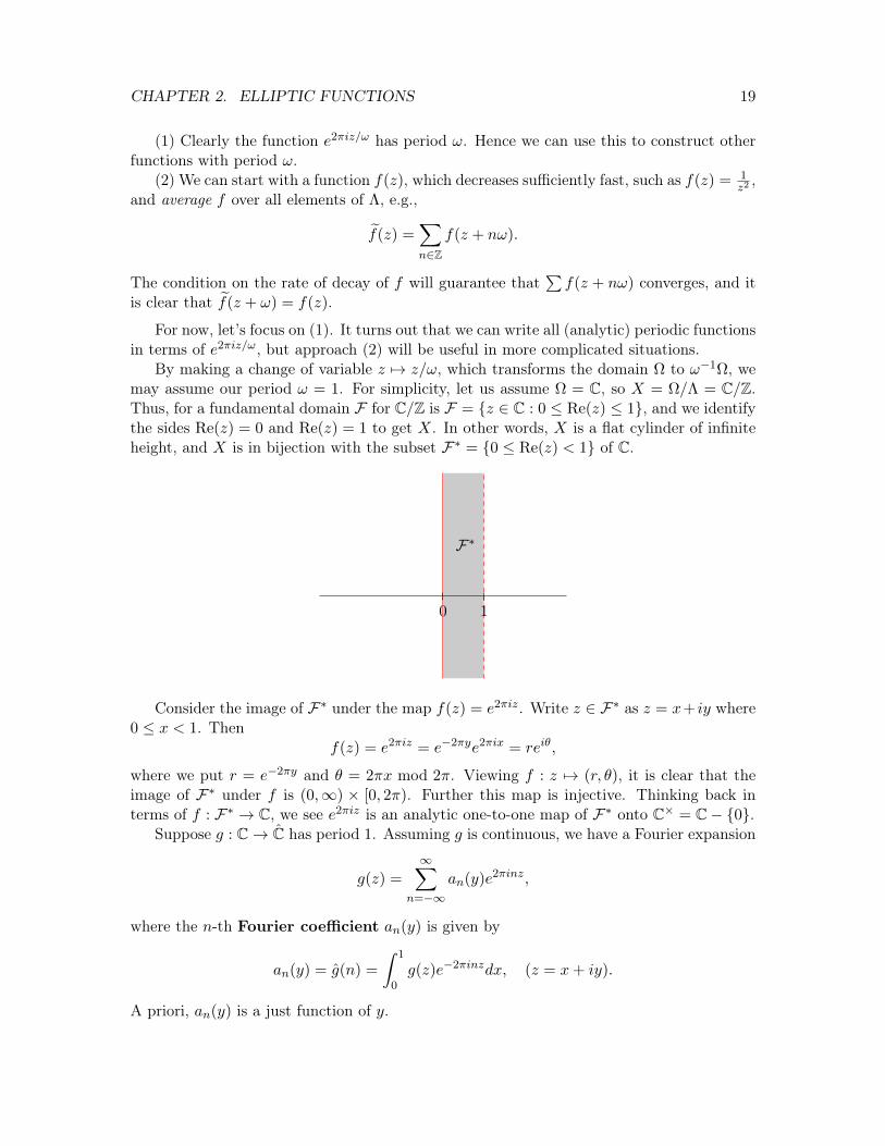
By making a change of variable z 7→ z/ω, which transforms the domain Ω to ω−1Ω, wemay assume our period ω = 1. For simplicity, let us assume Ω = C, so X = Ω/Λ = C/Z.Thus, for a fundamental domain F for C/Z is F = z ∈ C : 0 ≤ Re(z) ≤ 1, and we identifythe sides Re(z) = 0 and Re(z) = 1 to get X. In other words, X is a flat cylinder of infiniteheight, and X is in bijection with the subset F∗ = 0 ≤ Re(z) < 1 of C.
F∗
10
Consider the image of F∗ under the map f(z) = e2πiz. Write z ∈ F∗ as z = x+ iy where0 ≤ x < 1. Then
f(z) = e2πiz = e−2πye2πix = reiθ,
where we put r = e−2πy and θ = 2πx mod 2π. Viewing f : z 7→ (r, θ), it is clear that theimage of F∗ under f is (0,∞) × [0, 2π). Further this map is injective. Thinking back interms of f : F∗ → C, we see e2πiz is an analytic one-to-one map of F∗ onto C× = C− 0.
Suppose g : C→ C has period 1. Assuming g is continuous, we have a Fourier expansion
g(z) =
∞∑n=−∞
an(y)e2πinz,
where the n-th Fourier coefficient an(y) is given by
an(y) = g(n) =
∫ 1
0g(z)e−2πinzdx, (z = x+ iy).
A priori, an(y) is a just function of y.

CHAPTER 2. ELLIPTIC FUNCTIONS 20
However if g is meromorphic, then we have a stronger result. Put ζ = f(z). Thenthere is a unique meromorphic G : C× → C such that g(z) = G(ζ). It is natural to askwhen G extends to a meromorphic function of C. By Theorem 2.2.5, this is if and onlyif limζ→0G(ζ)|ζ|m = 0 for some m. Note that ζ = e2πiz → 0 for z ∈ F∗ if and only ifIm(z)→∞. Hence we may restate the above condition on G(ζ) being meromorphic at 0 aslimIm(z)→∞ g(z)|e2πimz| → 0 for some m, i.e.,
for Im(z) large, there exists m such that |g(z)| < e2πmy. (2.3.1)
Since ζ → 0 corresponds to Im(z) → ∞, we say g is meromorphic at i∞ if (2.3.1) issatisfied.
Assume now that g is also meromorphic at i∞. Then G(ζ) has a Laurent series expansionabout 0,
g(z) = G(ζ) =
∞∑n=−m
cnζn =
∞∑n=−m
cne2πinz,
where m is the order of the pole of G at 0. (We can take m = 0 if G does not have a poleat 0.) This must agree with the Fourier expansion above, so we have an(y) = cn for alln ≥ −m and an(y) ≡ 0 for n < −m. Hence for meromorphic periodic functions, the Fouriercoefficients are constant (independent of y) and all but finitely many of the negative Fouriercoefficients vanish.
These facts about the Fourier expansion will be crucial in our study of modular forms.
2.4 Doubly periodic functions
Let ω1, ω2 be two complex periods, i.e., two nonzero complex numbers linearly independentover R. Then they generate a lattice Λ = 〈ω1, ω2〉 = aω1 + bω2 : a, b ∈ Z ⊂ C. We mightpicture Λ as “parallelogram grid” follows.
ω1
ω2
ω1 + ω2
0
While technically the lattice Λ is only the set of vertices of the above parallelogram grid,it is convenient to draw it as above.

CHAPTER 2. ELLIPTIC FUNCTIONS 21
Definition 2.4.1. A meromorphic function f : C → C is elliptic (or doubly periodic)with respect to Λ if
f(z + ω) = f(z) for all z ∈ C, ω ∈ Λ.
The space of all such functions is denoted E(Λ).
Note f ∈ E(Λ) if and only if f(z + ω1) = f(z + ω2) = f(z). As with singly periodicfunctions, we can identify doubly periodic functions with functions on a quotient spaceC/Λ. Note this quotient space is a (flat) torus. We can take for a fundamental domain Fthe (closed) parallelogram whose vertices are drawn above.
ω1
ω2
ω1 + ω2
0
F
Then C/Λ is identified with the torus obtained by gluing together both opposite pairsof edges of the fundamental parallelogram F .
We remark that elliptic functions were originally studied because they contain, as aspecial case, the inverse functions of the classical elliptic integrals (integrals involving thesquare root of a cubic or quartic polynomial, which arise in the problem of finding the arclength of certain elliptical shapes, such as spirals and cycloids). This is also, as you mayguess, the root of the modern terminology.
We would like to be able to describe the space of meromorphic functions on C/Λ. Earlier,we suggested two methods for constructing periodic functions: (1) write functions in termsof a simple periodic function you know; and (2) average functions over Λ. Since there areno obvious nonconstant doubly periodic functions, here we’ll start with approach (2).
In order to get something that converges, we need to average a function that decayssufficiently fast. A first idea might be to try averaging 1
z2over the lattice Λ = 〈1, i〉. This
would be ∑ω∈Λ
1
(z + ω)2=∑a,b∈Z
1
(z + (a+ bi)2). (2.4.1)
If this converges, it would have a pole of order 2 at each lattice point, and nowhere else.However, it does not converge (absolutely). To see this, take z = 0, and sum up the absolutevalues of all terms excluding the 1
z2term to get∑
(a,b)∈Z2−(0,0)
1
|a+ bi|2=∑a,b
1
a2 + b2≈ 4
∫ ∞1
∫ ∞1
dx dy
x2 + y2≈∫ 2π
0
∫ ∞1
r dr dθ
r2=∞.
CHAPTER 2. ELLIPTIC FUNCTIONS 22
(Here of course the approximations are certainly good enough to formally check divergenceof the right most integral implies divergence of the sum on the left.)
Since (2.4.1) does not converge absolutely, the next simplest idea would be to consider
g(z) =∑ω∈Λ
1
(z + ω)3.
Indeed this sum converges absolutely, except of course when z ∈ Λ, in which case we geta pole of order 3. However, it turns out that one can modify the sum in (2.4.1) to getan elliptic function with only poles of order 2 at each lattice point. Precisely, we defineWeierstrass pe function (with respect to Λ) to be
℘(z) =1
z2+
∑ω∈Λ−0
(1
(z + ω)2− 1
ω2
).
This can be shown to converge and although not as obvious as (2.4.1), to be doubly periodic(see exercises below). Given this, it is clear this has a pole of order 2 at each z ∈ Λ and nopoles elsewhere, so ℘ is an elliptic function of order 2. (The order of an elliptic function isthe sum of the orders of its poles in C/Λ.)
Since ℘ is analytic on C− Λ, it is differentiable, and on checks that its derivative is
℘′(z) = −2g(z) = −2∑ω∈Λ
1
(z + ω)3, (2.4.2)
which has order 3.
Exercise 2.4.2. Show ℘(z) converges absolutely for z 6∈ Λ and uniformly on compact setsin C− Λ.
Exercise 2.4.3. Verify Equation (2.4.2).
Exercise 2.4.4. Use the previous exercise together with the fact that ℘ is even to show ℘is elliptic with respect to Λ.
Now one might ask: are there any (nonconstant) elliptic functions of order 0 or 1? Abasic result of complex analysis is the following.
Theorem 2.4.5. (Liouville) Any bounded entire function is constant.
If f ∈ E(Λ) has no poles, then it must be holomorphic on C, i.e., entire. Further the onlyvalues attained by f are the ones attained by restricting f to the fundamental parallelogramF , so f is also bounded. This shows there are no nonconstant elliptic functions of order 0(⇐⇒ holomorphic).
Furthermore, one can show there are no elliptic functions of order 1. For those of youwho remember your complex analysis, the argument goes as follows. The double periodicitycondition, together with Cauchy’s theorem, implies that the integral around any fundamentalparallelogram with no poles on the border must be 0. (We may assume by shifting ourfundamental domains that there are no poles on these parallelograms.) Hence by the residue

CHAPTER 2. ELLIPTIC FUNCTIONS 23
theorem, the sum of the residues in any parallelogram must be 0. In particular, we cannothave only one simple pole inside such a parallelogram.
The point is that ℘ is the simplest (nonconstant) elliptic function. Furthermore, it is nottoo difficult to show that the space of elliptic functions E(Λ) is a field, and it is generatedby ℘ and ℘′, i.e.,
E(Λ) = C(℘, ℘′),
i.e., any elliptic function can be expressed as a rational function in ℘ and ℘′.
2.5 Elliptic functions to elliptic curves
The theory of elliptic functions gave rise to the modern theory of elliptic curves and tomodular forms. This is very beautiful and important mathematics, so despite the fact thatit will not be so relevant to our treatment of modular forms, I feel obliged to at leastsummarize these connections.
In this section, x and y do not denote the real and imaginary parts of a complex numberz.
Definition 2.5.1. Let F be a field. An elliptic curve over F is a nonsingular (smooth)cubic curve in F 2.
We won’t give a precise definition of nonsingular, but by cubic curve we mean a curvedefined by a cubic polynomial (in this case, in two variables).
Theorem 2.5.2. Let F be a field of characteristic zero and E/F be an elliptic curve. Then,up to a change of variables, we may express E in Weierstrass form as
y2 = x3 + ax+ b, (a, b ∈ F ).
Furthermore, an equation of the above type defines an elliptic curve if and only if the dis-criminant ∆ = ∆(E) = −16(4a3 + 27b2) 6= 0.
The nonzero discriminant condition is what forces the equation to be nonsingular. E.g.,the equation y2 = x3 has a cusp at the origin (graph it over R).
Actually, one typically wants to consider projective elliptic curves rather than just theaffine curves. Suffice it to say that, for a curve in Weierstrass form, the projective ellipticcurve can be thought of as the affine curve given above together with a point at infinity. Itis well known that the points of an elliptic curve form an abelian group, with the point atinfinity being the identity element. However to prove it directly from the above definitionis not so easy.
Let Λ = 〈ω1, ω2〉 be a period lattice in C, and ℘ be the associated Weierstrass pe function.Then for all z ∈ C− Λ,
℘′(z)2 = 4℘(z)3 − 60G4℘(z)− 140G6,
where Gk =∑
ω∈Λ−0 ω−k. In other words, the map z 7→ (℘(z), ℘′(z)) maps C onto (the
affine points) of the elliptic curve EΛ : y2 = 4x3 − 60G4x− 140G6 defined over C, assuming

CHAPTER 2. ELLIPTIC FUNCTIONS 24
Λ is chosen so that the discriminant of Eλ is nonzero. (Replacing y with 2y puts this inWeierstrass form, if one wishes to do that.) By the periodicity of ℘ and ℘′, this factorsthrough (C − Λ)/Λ. We extend this map to C/Λ by sending Λ to the point at infinity onEΛ.
This map gives an analytic isomorphism
C/Λ ' EΛ
from the torus C/Λ to the elliptic curve EΛ. Furthermore, all elliptic curves over C (andconsequently all elliptic curves over any subfield of C) arise from some such lattice Λ. Con-sequently all (projective) elliptic curves over C are topologically tori. Now it is clear thatthe points on the (projective) elliptic curve EΛ naturally form an additive group becauseC/Λ is (with respect to addition on C, taken modulo Λ), and the identity of EΛ is the pointat infinity, which corresponds to the identity Λ of (C/Λ,+) by construction.
Hence elliptic functions (particularly ℘ and ℘′) provide a link between lattices in C andcomplex elliptic curves. We will now sketch how elliptic functions and elliptic curves leadto the theory modular forms.
We say two lattices Λ and Λ′ in C are equivalent if Λ′ = λΛ for some λ ∈ C×.
Exercise 2.5.3. Show that if Λ and Λ′ are equivalent, the elliptic functions on Λ′ are simplythe elliptic functions on Λ composed with a simple change of variables.
Furthermore, Λ and Λ′ being equivalent is the same as the elliptic curves EΛ and EΛ′
being group isomorphic by an analytic map.Write Λ = 〈ω1, ω2〉. Clearly Λ is equivalent to the lattice 〈1, τ〉 where τ = ω2/ω1. Since
〈1, τ〉 = 〈1,−τ〉 and τ 6∈ R, we may assume Im(τ) > 0, i.e., τ lies in the upper half-planeH = z ∈ C : Im(z) > 0.
For τ, τ ′ ∈ H, the lattices 〈1, τ〉 and 〈1, τ ′〉 are equal if and only if τ ′ ∈ 〈1, τ〉 andτ ∈ 〈1, τ ′〉, i.e., if and only if τ ′ = aτ + b and τ = cτ ′ + d for some a, b, c, d ∈ Z. It is easyto see this means τ ′ = τ + b for some b ∈ Z.
Hence we may assume τ ∈ H/Z, or more precisely, −12 ≤ Re(τ) < 1
2 . This means that±1,±τ will be the four nonzero lattice points of 〈1, τ〉 closest to the origin. Hence theonly way two lattices 〈1, τ〉 and 〈1, τ ′〉 can be equivalent is if λ ±1,±τ = ±1,±τ ′. It isnot hard to see this means either τ ′ = τ or τ ′ = − 1
τ .
Exercise 2.5.4. Let τ, τ ′ ∈ H. Fill in the details in the above argument to show that 〈1, τ〉and 〈1, τ ′〉 are equivalent if and only if τ ′ = τ + b or τ ′ = − 1
τ + b, for some b ∈ Z.
What the above shows is that equivalence classes of lattices are parametrized by the setof τ ∈ H subject to the conditions either −1
2 ≤ Re(τ) < 12 and |τ | > 1 or −1
2 ≤ Re(τ) ≤ 0and |τ | = 1.

CHAPTER 2. ELLIPTIC FUNCTIONS 25
−12
12
We will see in the next section that the (closure of the) above region is a fundamentaldomain for Γ\H, where Γ ' PSL(2,Z) is the group of (hyperbolic) isometries of H generatedby the transformations τ 7→ τ + 1 and τ 7→ − 1
τ .What does all this have to do with modular forms? Well, if you are studying elliptic
curves (or even just lattices), one thing you want to look is invariants. For example, givenτ ∈ H, consider the map
∆ : τ 7→ Λ = 〈1, τ〉 7→ EΛ 7→ ∆(Eλ),
sending a point in H to the discriminant of the associated elliptic curve. Equivalent (an-alytically group isomorphic) elliptic curves have essentially the same discriminant, so ∆ isa (holomorphic) function on H satisfying certain transformation properties under Γ. Theseproperties will make ∆ what is called a modular form of weight 12 and level 1.

Chapter 3
The Poincaré upper half-plane
There are two basic kinds of non-Euclidean geometry: spherical and hyperbolic. Sphericalgeometry is easy enough to imagine. Consider the sphere S2 =
(x, y, z) ∈ R3 : x2 + y2 + z2 = 1
.
Then the geodesics (paths which locally minimize distance) are simply the great circles. Inother words, for two points P and Q on S2, a shortest path in S2 between them is anarc lying on a great circle connecting P and Q (this great circle will be unique providedP 6= −Q), and the distance between P and Q in S2 is the (Euclidean) length of this arc.
Hyperbolic geometry is a bit harder to picture. Perhaps the easiest way to initiallyvisualize the hyperbolic plane is one sheet of the two-sheeted hyperboloid x2 + y2 − z2 = 1,however this is not the easiest model to work with for many purposes. Just like with theEuclidean plane, the hyperbolic plane has translations, rotations and reflections. The twomost common models to use, both named after Poincaré, are the Poincaré disc model (dueto Beltrami) and the Poincaré upper half-plane model (due to Riemann). The disc modelhas the advantage of making rotations easy to visualize, and the upper half-plane model hasthe advantage of making translations easy to visualize. When working with modular forms,one always uses the upper half-plane model.
3.1 The hyperbolic plane
Unless stated otherwise, in this chapter z, w ∈ H and x, y ∈ R>0.
Definition 3.1.1. The Poincaré upper half-plane, or hyperbolic plane, is the set
H = z ∈ C : Im(z) > 0
together with the metric given by the distance function
d(z, w) = cosh−1
(1 +
|z − w|2
2 Im(z) Im(w)
).
Angles in the hyperbolic plane H are just taken to be the usual Euclidean angles.We will often write
d(z, w) = cosh−1
(1 +
u(z, w)
2
),
26
CHAPTER 3. THE POINCARÉ UPPER HALF-PLANE 27
where
u(z, w) =|z − w|2
Im(z) Im(w).
While modular forms will be functions on H satisfying certain transformation laws underisometry groups, we do not actually need to know too much about the geometry of H forour study of modular forms. Thus some basic facts about the geometry of H which we donot need, but may help conceptually to be aware of, I will just state without proof. Insteadone may refer to basic references on hyperbolic geometry, such as [And05] or [Kat92].
The first such fact is the following.
Lemma 3.1.2. d(z, w) is a metric on H.
To see why this is plausible, first notice the argument of cosh−1 always lies in [1,∞).Recall cosh(x) = ex+e−x
2 so cosh(0) = 1 and cosh is increasing and concave up on [0,∞). Socosh−1(1) = 0 and cosh−1 is increasing and concave down on [1,∞) (it grows logarithmicallyof course).
In particular, (i) d(z, w) : H × H → [0,∞) with d(z, w) = 0 if and only if the argumentof cosh−1 is 1, i.e., if and only if u(z, w) = 0, i.e., if and only if z = w. It is also clearthat (ii) d(z, w) = d(w, z) for z, w ∈ H since u(z, w) = u(w, z). Thus to show d(z, w) isa metric, it remains to show (iii) the triangle inequality, d(z, w) ≤ d(z, v) + d(v, w), holdsfor all z, w, v ∈ H. This is somewhat technical (and more easily proven using a differentformulation of the hyperbolic distance), so I’ll leave it to you to either work out or look up.
Another fact one should know, though not formally used in our development of modularforms is the following.
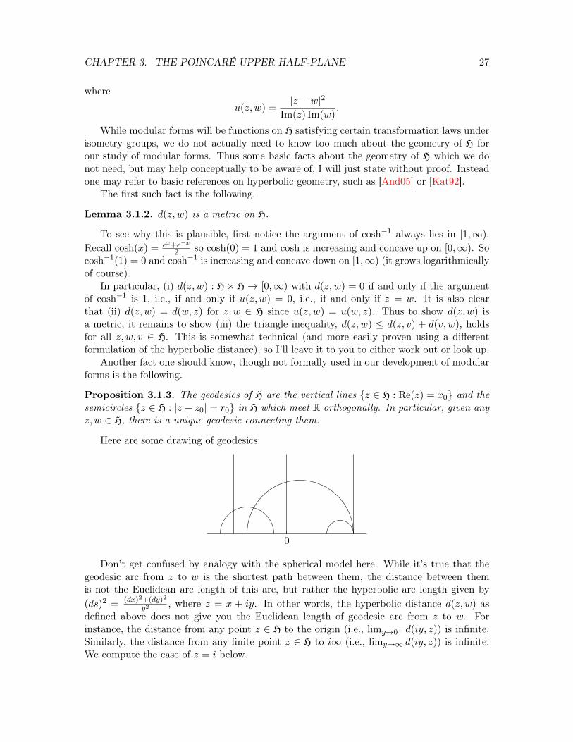
Proposition 3.1.3. The geodesics of H are the vertical lines z ∈ H : Re(z) = x0 and thesemicircles z ∈ H : |z − z0| = r0 in H which meet R orthogonally. In particular, given anyz, w ∈ H, there is a unique geodesic connecting them.
Here are some drawing of geodesics:
0
Don’t get confused by analogy with the spherical model here. While it’s true that thegeodesic arc from z to w is the shortest path between them, the distance between themis not the Euclidean arc length of this arc, but rather the hyperbolic arc length given by(ds)2 = (dx)2+(dy)2
y2, where z = x + iy. In other words, the hyperbolic distance d(z, w) as
defined above does not give you the Euclidean length of geodesic arc from z to w. Forinstance, the distance from any point z ∈ H to the origin (i.e., limy→0+ d(iy, z)) is infinite.Similarly, the distance from any finite point z ∈ H to i∞ (i.e., limy→∞ d(iy, z)) is infinite.We compute the case of z = i below.
CHAPTER 3. THE POINCARÉ UPPER HALF-PLANE 28
Example 3.1.4. Let y ∈ R>0. Then
d(i, iy) = cosh−1
(1 +
(y − 1)2
2y
)In fact, since cosh−1(x) = ln(x+
√x+ 1
√x− 1), we can write
d(i, iy) = ln
(y2 + 1
2y+|y2 − 1|
2y
)= | ln y|.
In particular, we see iy and i/y are equidistant from i, and indeed d(i, 0) := limy→0+ d(i, iy) =∞ = limy→∞ d(i, iy) =: d(i, i∞). Applying the triangle inequality shows in fact d(z, 0) =d(z, i∞) =∞ for any z ∈ H.
Exercise 3.1.5. For x, y > 0, compute the hyperbolic distance d(ix, iy).
Exercise 3.1.6. For z = eiθ ∈ H, compute the hyperbolic distance d(i, z).
3.2 Fractional linear transformations
In this section, z will denote an element of H, x = Re(z) and y = Im(z) > 0.One nice thing about the upper half-plane model is that there is a nice way to de-
scribe the isometries of H in terms of fractional linear transformations (also called Möbiustransformations), which you may have encountered in complex analysis.
Recall for a ring R, we may define the 2× 2 special linear group
SL2(R) :=
(a bc d
): a, b, c, d ∈ R, ad− bc = 1
,
as well as the corresponding projective special linear group
PSL2(R) := SL2(R)/Z,
where Z denotes the (central) subgroup of scalar matrices of SL2(R), i.e.,
Z =
(a
a
)∈ SL2(R)
=
(a
a
): a ∈ R, a2 = 1
.
(If you’re not familiar with these, check that these are groups.) The most important casesfor us in this course are R = R and R = Z; in both of these cases Z = ±I.
Definition 3.2.1. A fractional linear transformation of H is a map H→ C of the form(a bc d
)z =
az + b
cz + d, z ∈ H
where(a bc d
)∈ SL2(R).

CHAPTER 3. THE POINCARÉ UPPER HALF-PLANE 29
(More generally, one can consider fractional linear transformations(a bc d
)∈ GL2(C),
but we will always mean elements of SL2(R) by the term fractional linear transformation.)First note that, for c, d ∈ R not both 0, z → az+b
cz+d is a rational function of C with at mostone pole (of order 1) at −d/c ∈ R if c 6= 0, fractional linear transformations are holomorphicmaps from H to C.
Exercise 3.2.2. Show that the image of H under a linear fractional transformation is con-tained in H.
This allows us to compose fractional linear transformations on H.
Lemma 3.2.3. For σ, τ ∈ SL2(R), the fractional linear transformation σ τ : H→ H givenby their composition is equal to the fractional linear transformation στ given by their matrixproduct.
The proof is just a simple computation, which we relegate to
Exercise 3.2.4. Prove Lemma 3.2.3.
Lemma 3.2.5. Let τ ∈ SL2(R). The fractional linear transformation τ : H→ C in fact ananalytic automorphism τ : H → H, i.e., τ : H → H an analytic bijection whose inverse isalso analytic. Further, τ acts trivially on H if and only if τ = ±I.
Proof. Write τ =
(a bc d
). Then
τ(z) =ax+ aiy + b
cx+ ciy + d· cx+ d− ciycx+ d− ciy
=(ad+ bc)x+ bd+ acy2 + iy(ad− bc)
(cx+ d)2 + (cy)2
Since ad− bc = 1, we have(a bc d
)z =
(ad+ bc)x+ bd+ acy2 + iy
(cx+ d)2 + (cy)2=
(ad+ bc)x+ bd+ acy2 + iy
|cz + d|2, (3.2.1)
which clearly has positive imaginary part, so τ(H) ⊆ H.To see this is one-to-one, suppose τ(z) = τ(w) for z, w ∈ H. Then cross-multiplying
denominators and expanding out
az + b
cz + d=aw + b
cw + d
givesadz + bcw = adw + bcz,
which says(ad− bc)z = (ad− bc)w,
i.e., z = w.Note the identity of SL2(R) acts trivially on H. By the previous lemma, this means
τ−1 τ acts trivially on H. In particular, τ maps onto H. Hence τ : H → H is an analyticautomorphism.

CHAPTER 3. THE POINCARÉ UPPER HALF-PLANE 30
In order for τ to be the identity on H, looking at the imaginary part of τ(z) shows(cx + d)2 + (cy)2 = 1 for all x ∈ R and y > 0. This implies c = 0 and d = ±1. Then thereal part of τ(z) is simply adx+ bd. For this to always equal x, we need b = 0 and ad = 1.Hence τ = ±I are the only elements of SL2(R) which act trivially on H.
So from now on, we will view fractional linear transformations as analytic automorphismson H (i.e., holomorphic bijections from H to H whose inverses are also holomorphic).
Because composition respects group multiplication, and the only fractional linear trans-formations acting trivially are ±I, two elements σ, τ ∈ SL2(R) define the same map if andonly if σ = ±τ . This means we can identify the group of fractional linear transformationson H with PSL2(R). Despite the fact that elements of PSL2(R) are technically not 2 × 2matrices, we will still write elements of PSL2(R) as elements of SL2(R) with the conventionthat −τ is identified with τ .
Now let’s look at a few specific examples of fractional linear transformations. Let
τn =
(1 n
1
),
δm2 =
(m
m−1
), and
ι =
(1
−1
).
Then
τn(z) =
(1 n
1
)z = z + n
simply translates H to the right by n,
δm2(z) =
(m
m−1
)z = m2z
dilates, or scales, H outward radially from the origin by m2, and
ι(z) =
(1
−1
)z = −1
z
inverts H about the semicircle z ∈ H : |z| = 1. (Writing z = reiθ may make these lattertwo transformations easier to visualize. The second then becomes obvious, and we seeι(reiθ) = 1
rei(π−θ).) Note all these transformations map geodesics to geodesics. Furthermore,
because they are holomorphic maps, they are conformal, i.e., they preserve angles.
Lemma 3.2.6. The group of fractional linear transformations PSL2(R) acts transitively onH, i.e., for any z, w ∈ H, there exists τ ∈ H such that τ(w) = z.
Proof. It suffices to show that for any z ∈ H, there exists τ ∈ PSL2(R) such that τ(i) = z.For then there also exists σ ∈ PSL2(R) such that σ(i) = w, so (τσ−1)(w) = z by theprevious lemma.
Write z = x+ iy with x, y ∈ R and let τ = τxδy. Then τ(i) = τx(iy) = x+ iy = z.
CHAPTER 3. THE POINCARÉ UPPER HALF-PLANE 31
A basic fact, though we will not need it, is the following.
Proposition 3.2.7. The group PSL2(R) of fractional linear transformations on H is pre-cisely the group of orientation-preserving isometries of H.
(To obtain the orientation-reversing isometries, one considers 2× 2-matrices of determi-nant −1.)
We note that since angles in H are simply Euclidean angles, the fact that holomorphicmaps are conformal implies fractional linear transformations preserve hyperbolic angles.
While we omit the proof, we remark that it is straightforward (though somewhat tedious)to check that all fractional linear transformations are isometries, i.e., they preserve distance,i.e., d(z, w) = d(τ(z), τ(w)) for z, w ∈ H and τ ∈ PSL2(R). However the computations aresimpler in the following case.
Exercise 3.2.8. Let τ ∈ PSL2(R) and z ∈ H. Show d(z, i) = d(τ(z), τ(i)). (Note it sufficesto show u(z, i) = u(τ(z), τ(i)).)
From now on, we will often write τ(z) simply as τz for τ ∈ PSL2(R).
3.3 The modular group
In this course, we will not work with the group of all fractional linear transformationsPSL2(R), but rather certain nice discrete subgroups Γ. First we will study the most basicdiscrete subgroup, the (full) modular group, PSL2(Z).
(Some authors call SL2(Z) the full modular group because they prefer to work in termsof matrices, but we prefer to think in terms of fractional linear transformations of H, soPSL2(Z) is more natural to work with. However, there is no difference between speciallinear groups and projective linear groups in terms of fractional linear transformations, sothis should not cause any confusion.)
Proposition 3.3.1. PSL2(Z) = 〈S, T 〉 where S =
(1
−1
)and T =
(1 1
1
).
Note that S and T are simply the inversion ι and translation τ1 defined in the previoussections, however the notation of S and T is standard for these specific matrices.
Proof. Let Γ = 〈S, T 〉. It is clear Γ ⊆ PSL2(Z). Note also that T ∈ Γ implies
N =
(1 x
1
): x ∈ Z
⊆ Γ.
Similarly
N =
(1y 1
): y ∈ Z
⊆ Γ,
since N is generated by T = S−1TS =
(1−1 1
)∈ Γ.

CHAPTER 3. THE POINCARÉ UPPER HALF-PLANE 32
Now let(a bc d
)∈ PSL2(Z). We want to show
(a bc d
)∈ Γ. First note that
S−1
(a bc d
)S =
(d −c−b a
),
we may assume |a| ≤ |d|. Next observe(a bc d
)(1 x
1
)=
(a ax+ bc cx+ d
).
Hence by multiplying(a bc d
)on the right by some element ofN , we may assume 0 ≤ b < |a|.
Similarly, since (1y 1
)(a bc d
)=
(a b
ay + c by + d
),
we may also assume 0 ≤ c < |a|. Hence ad and bc are integers such that ad − bc = 1,|ad| ≥ a2 and |bc| < a2. So we must have ad = 1 and bc = 0. In particular, a = d = ±1,and 0 ≤ b < |a| and 0 ≤ c < |a| then means b = c = 0, i.e.,(
a bc d
)= ±
(1 0
1
)∈ Γ.
Remark. One can show in fact 〈S, T |S2 = (ST )3 = 1〉 is a presentation for PSL2(Z).
We have already defined the notion of a fundamental domain for Ω/Λ, where Ω ⊂ Cand Λ is a group of (Euclidean) isometries of Ω. We define fundamental domains in thehyperbolic plane the same way. For formality’s sake, we write out the definition now.
Definition 3.3.2. Let F ⊂ H be a closed set with connected interior, and Γ a subgroup ofPSL2(Z). We say F is a fundamental domain for Γ (or Γ\H) if
(i) any z ∈ H is Γ-equivalent to some point in F ;(ii) no two interior points of F are Γ-equivalent; and(iii) the boundary ∂F of F is a finite union of smooth curves in H ∩ F .
To clarify for future use, by (ii) we mean that if z, z′ lie in the interior F0 of F such thatγz = z′ for γ ∈ Γ, then z = z′. We do not mean that γz = z′ implies γ = I. However, wewill see later (Lemma 3.5.1) that our interpretation of (ii) implies γ = I.
LetF =
z ∈ H : |Re(z)| ≤ 1
2, |z| ≥ 1
.

CHAPTER 3. THE POINCARÉ UPPER HALF-PLANE 33
0 12−1
21−1
F
i
ζ3 ζ6
(Here ζk = e2πi/k.)
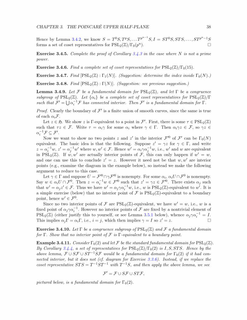
Proposition 3.3.3. F is a fundamental domain for PSL2(Z).
Proof. Condition (iii) of Defintion 3.3.2 (∂F is a finite union of smooth curves) is obviouslysatisfied, so we just need to show the first two conditions.
First we show (i) any point z ∈ H is PSL2(Z)-equivalent to some point in F , i.e., for any
z ∈ H, there is some γ =
(a bc d
)∈ PSL2(Z) such that γz ∈ F . Observe that by (3.2.1), we
have Im(γz) = Im(z)|cz+d|2 . Since c, d ∈ Z and they are not both 0, |cz + d|2 attains a minimum
as γ ranges over PSL2(Z). Consequently, we may choose γ such that Im(γz) is maximal.Replacing γ by Tnγ for some n ∈ Z shows that we may further assume |Re(γz)| ≤ 1
2 .It remains to show |γz| ≥ 1. Suppose not. Let w = γz and write w = u+ iv. Then
Sw =−u+ iv
u2 + v2.
In particular, if |w| < 1, then Im(Sw) > Im(w), i.e., Im(Sγz) > Im(γz), contradicting themaximality of Im(γz). This proves (i).
Now we need to show (ii) no two interior points of F are PSL2(Z)-equivalent. Suppose
z and w lie in the interior of F , and γz = w for some γ =
(a bc d
)∈ PSL2(Z). We may
assume Im(w) ≥ Im(z), or else we could switch z and w and replace γ by γ−1. SinceIm(w) = Im(z)
|cz+d|2 , this means |cz + d| ≤ 1. In particular |Im(cz + d)| = |c|Im(z) < 1, but
z ∈ F implies Im(z) >√
32 so |c| < 2.
First suppose c = 0. Then ad− bc = ad = 1. Multiplying γ by ±1 if necessary (recall weare working in PSL2(Z), so this does not change γ), we may assume a = d = 1 so γ = Tn
for some n ∈ Z. In this case it is clear we cannot have γz ∈ F .

CHAPTER 3. THE POINCARÉ UPPER HALF-PLANE 34
Now suppose c = ±1. Multiplying γ by ±1 if necessary, we may assume c = 1. Note
1 > |cz + d|2 = Re(z + d)2 + Im(z)2 > Re(z + d)2 +3
4.
Hence |Re(z + d)| < 12 , which implies d = 0 since |Re(z)| < 1
2 . Then the determinantcondition implies b = −1. So
γ =
(a −11 0
),
i.e., γz = a− 1z , which cannot lie in F . This proves (ii).
Recall when we defined the notion of a fundamental domain, we said some authorsrequire fundamental domains to be convex. Note that F is convex in H (with respectto the hyperbolic metric), i.e., given any two points in F , one can connect them with aunique geodesic segment, and that segment—either a vertical line segment or a segment ofa semicircle centered on the real line—lies entirely in F .
Exercise 3.3.4. Show two boundary points z, z′ of F are PSL2(Z)-equivalent if and only ifIm(z) = Im(z′) and Re(z) = −Re(z′).
The above exercise shows the quotient space PSL2(Z)\H parametrizes equivalence classesof lattices as described Section 2.5 (cf. figure at end of Section 2.5). (Note, in contrast toChapter 2, it is standard to write the quotient by the action of PSL2(Z) on the left herebecause we think of matrices as acting on H from the left.)
Since the fundamental domain F we have given above is universally used, it is calledthe standard fundamental domain for PSL2(Z). There is a trivial way to cook upother fundamental domains—namely γF is also a fundamental domain for PSL2(Z) for anyγ ∈ PSL2(Z). This statement is slightly generalized in the following simple exercise.
Exercise 3.3.5. Let Γ ⊆ PSL2(R) be discrete and suppose F ′ is a fundamental domain forΓ. Suppose γ ∈ PSL2(R) such that γ−1Γγ = Γ. Show γF ′ is also a fundamental domain forΓ.
*Exercise 3.3.6. (i) Show that the set of γF with γ ∈ PSL2(Z) tile H, i.e., their unioncovers H and their interiors are pairwise disjoint.
(ii) Show the picture below of the partial tiling of H given by γF is correct, where welabelled the region γF simply by γ. (Hint: begin by showing S takes the vertical line x+iR>0
to the upper semicircle passing through 0 and − 1x .)

CHAPTER 3. THE POINCARÉ UPPER HALF-PLANE 35
0 12−1
21−1 2−2 1
323
IT−1 T
ST−1S TS
ST−1STSTS TST
In the above diagram, note STS = T−1ST−1 and TST = ST−1S.
3.4 Congruence subgroups
From our point of view so far, the simplest kinds of (meromorphic) modular forms (modularfunctions of level one) will be meromorphic functions f : H→ C satisfying
f(γz) = f(z) for γ ∈ PSL2(Z). (3.4.1)
Note this is a hyperbolic analogue of the definition of elliptic functions. Specifically, fixa lattice Λ ⊂ C and let ΓΛ be the group of isometries of C given by γω(z) = z + ω where ωranges over Λ. Then elliptic functions w.r.t. Λ were simply defined to be the (meromorphic)functions on C satisfying f(γz) = f(z) for γ ∈ ΓΛ.
So instead of being functions on C (with Euclidean geometry) invariant under an isometrygroup ΓΛ corresponding to a lattice Λ, modular functions will be functions on H (withhyperbolic geometry) invariant under a hyperbolic isometry group Γ, with the simplest casebeing Γ = PSL2(Z).
If one wants to think of a hyperbolic analogue of the lattice Λ, there is no issue here.Note one can recover the lattice Λ ⊂ C from the group ΓΛ simply by looking at the ΓΛ-translates of the origin in C. In this way, we see any isometry group of C isomorphic toZ× Z gives a lattice. Similarly, for any (noncyclic) “discrete” isometry group Γ ⊂ PSL2(R)of H, one can think of the corresponding “hyperbolic lattice” as simply the Γ-translates ofi. (Note discrete here precisely means the Γ-translates of i form a discrete subset of H, andone excludes the case of cyclic groups Γ as they will correspond to “1-dimensional” latticesin H.)
Now the modular functions satisfying (3.4.1), while certainly very interesting, are notsufficient for most number theoretic purposes. There are two ways of generalizing (3.4.1)that will include many import functions arising naturally in number theory. One way is toloosen the invariance by only requiring f(γz) = α(γ, z)f(z) for some “weight” α(γ, z) (thenone calls the resulting functions modular forms). The second way is to not require (3.4.1)

CHAPTER 3. THE POINCARÉ UPPER HALF-PLANE 36
hold for all γ ∈ PSL2(Z), but merely all γ ∈ Γ, where Γ is a suitable subgroup of PSL2(Z).In fact, as alluded to earlier, one could just require that Γ be a noncyclic discrete subgroupof PSL2(R). However the most interesting cases of study for number theory is when Γ is acongruence subgroup of PSL2(Z).
Definition 3.4.1. Let N ∈ N. The modular group of level N is
Γ0(N) =
(a bc d
)∈ PSL2(Z) : c ≡ 0 mod N
.
Note when N = 1, we have Γ0(1) = PSL2(Z), and we sometimes call this the fullmodular group. It is also clear that
Γ0(N) ⊆ Γ0(M) if M |N.
One also has the more refined congruence subgroups
Γ1(N) =
(a bc d
)∈ PSL2(Z) :
(a bc d
)≡(
1 b0 1
)mod N
and the principal congruence subgroups
Γ(N) =
(a bc d
)∈ PSL2(Z) :
(a bc d
)≡(
1 00 1
)mod N
.
All of these subgroups are finite index inside PSL2(Z) and have been studied classicallyin the context of modular forms. Note that
Γ(N) ⊆ Γ1(N) ⊆ Γ0(N).
In general, a congruence subgroup of PSL2(Z) is a subgroup containing some Γ(N).However, the most important congruence subgroups are the modular groups Γ0(N), and wewill restrict our focus in this course to them.
Unless explicitly stated otherwise, from now on, Γ will always denote a congruence sub-group of PSL2(Z).
In order to understand the coset space PSL2(Z)/Γ0(N), it will be helpful to use the“projective line over Z/NZ.” For (a, c), (a′, c′) ∈ Z/NZ× Z/NZ, we write (a, c) ∼ (a′, c′) if(a′, c′) = (λa, λc) for some λ ∈ (Z/NZ)×. It is clear that ∼ is an equivalence relation. Wedenote the equivalence class of (a, c) by (a : c), and define the projective line
P1(Z/NZ) = (a : c)|a, c ∈ Z/NZ, gcd(a, c) = 1 .
Here by gcd(a, c) = 1, we mean that there exist a, c ∈ Z in the congruence classes a mod Nand c mod N such that gcd(a, c) = 1); or, alternatively, there exist r, s ∈ Z/NZ such thatar + cs ≡ 1 mod N .
Lemma 3.4.2. The coset space PSL2(Z)/Γ0(N) is finite, in bijection with P1(Z/NZ), and
a set of coset representatives is given by matrices of the form(a bc d
), where (a, c) ∈ Z× Z
such that (i) (a : c) ranges over P1(Z/NZ) and (ii) b, d are chosen such that ad− bc = 1.

CHAPTER 3. THE POINCARÉ UPPER HALF-PLANE 37
Proof. First observe that(a bc d
)∈(a′ b′
c′ d′
)Γ0(N) ⇐⇒
(d′ −b′−c′ a′
)(a bc d
)∈ Γ0(N).
By definition, this holds if and only if the lower left hand coefficient of the product on theright, a′c− c′a, is divisible by N . In other words, we have(
a bc d
)∈(a′ b′
c′ d′
)Γ0(N) ⇐⇒ a′c ≡ ac′ mod N.
Note that a pair of integers (a, c) can occur as a column of a matrix in PSL2(Z) if and onlyif ad− bc = 1 is solvable, i.e., if and only if gcd(a, c) = 1.
Hence the space of cosets PSL2(Z)/Γ0(N) is in bijection with the set of pairs (a, c) ∈Z/NZ×Z/NZ such that gcd(a, c) = 1 under the equivalence that (a, c) ≡ (a′, c′) ⇐⇒ a′c ≡ac′ mod N . It suffices to show that a′c ≡ ac′ mod N is equivalent to (a′, c′) = (λa, λc) forsome λ ∈ (Z/NZ×).
Clearly if (a′, c′) = (λa, λc), then a′c ≡ ac′ mod N . On the other hand, suppose(a, c), (a′, c′) ∈ Z × Z such that gcd(a, c) = gcd(a′, c′) = 1 and a′c ≡ ac′ mod N . WriteN = pn1
1 · · · pnkk . By the Chinese Remainder Theorem, Z/NZ ' Z/pn1
1 Z × · · · × Z/pnkk Z.Under this isomorphism, write a = (a1, . . . , ak) where ai ∈ Z/pnii Z, and do similarly for c,a′, and c′.
Then a′c ≡ ac′ mod N means a′ici ≡ aic′i mod pnii for each i. By the condition gcd(a, c) =1, we know pi cannot divide both ai and ci. Assume pi - ai, and say gcd(ci, p
nii ) = peii .
Then a′ici ≡ aic′i mod pnii means gcd(c′i, p
nii ) = peii so pi - a′i. Put λi = a′ia
−1i . Then
a′i = λiai and c′i = λici. Consequently λ = (λ1, . . . , λk) ∈ (Z/NZ)× such that (a′, c′) ≡(λa, λc) mod N .
Corollary 3.4.3. [PSL2(Z) : Γ0(N)] = N∏p|N
(1 + 1
p
), where p runs through the distinct
prime divisors of N .
Proof. First suppose N = pn. For any equivalence class (a : c), either a is divisible by p ornot. If not, we may rewrite this class as (λa : λc) = (1 : λc) where λ ≡ a−1 mod N . Thereare N choices for λc mod N , and all inequivalent. If p|a then p - c, so by the same argumentwe may rewrite (a : c) = (λa : 1). Since λa must be a multiple of p, there are N/p choicesfor λa, and they all give inequivalent classes. Thus the proposition holds when N = pn.
The proof for arbitraryN follows from the prime power case using the Chinese RemainderTheorem (see exercise below).
Corollary 3.4.4. Let p be a prime, and n ∈ N. Then a complete set of coset representativesof PSL2(Z)/Γ0(pn) is given by
T ipS =
(ip −11 0
): 0 ≤ i < pn−1
∪ST jS =
(1 0−j 1
): 0 ≤ j < pn
.
Proof. First check T iS and ST jS are given by the expressions above. Then observe theproof of Corollary 3.4.3 actually tells us that
P1(Z/pnZ) =
(ip : 1) : 0 ≤ i < pn−1∪ (1 : j) : 0 ≤ j < pn .
CHAPTER 3. THE POINCARÉ UPPER HALF-PLANE 38
Hence by Lemma 3.4.2, we know S = T 0S, T pS, . . . T pn−1
S, I = ST 0S, STS, . . . , ST pn−1S
forms a set of coset representatives for PSL2(Z)/Γ0(pn).
Exercise 3.4.5. Complete the proof of Corollary 3.4.3 in the case where N is not a primepower.
Exercise 3.4.6. Find a complete set of coset representatives for PSL2(Z)/Γ0(15).
Exercise 3.4.7. Find [PSL2(Z) : Γ1(N)]. (Suggestion: determine the index inside Γ0(N).)
Exercise 3.4.8. Find [PSL2(Z) : Γ(N)]. (Suggestion: see previous suggestion.)
Lemma 3.4.9. Let F be a fundamental domain for PSL2(Z), and let Γ be a congruencesubgroup of PSL2(Z). Let αi be a complete set of coset representatives for PSL2(Z)/Γsuch that F ′ =
⋃α−1i F has connected interior. Then F ′ is a fundamental domain for Γ.
Proof. Clearly the boundary of F ′ is a finite union of smooth curves, since the same is trueof each αiF .
Let z ∈ H. We show z is Γ-equivalent to a point in F ′. First, there is some τ ∈ PSL2(Z)such that τz ∈ F . Write τ = αiγ for some αi where γ ∈ Γ. Then αiγz ∈ F , so γz ∈α−1i F ⊆ F ′.Now we want to show no two points z and z′ in the interior F ′0 of F ′ can be Γ0(N)
equivalent. The basic idea is that the following. Suppose z′ = γz for γ ∈ Γ, and writez = α−1
i w, z′ = α−1j w′ where w,w′ ∈ F . Hence w′ = αiγα
−1j w, i.e., w′ and w are equivalent
in PSL2(Z). If w,w′ are actually interior points of F , this can only happen if w′ = w,and one can use this to conclude z′ = z. However it need not be that w,w′ are interiorpoints (e.g., examine the diagram in the example below), so instead we make the followingargument to reduce to this case.
Let γ ∈ Γ and suppose U = F ′0∩γF ′0 is nonempty. For some αi, αiU ∩F0 is nonempty.Say w ∈ αiU ∩ F0. Then z = α−1
i w ∈ F ′0 such that z′ = γz ∈ F ′0. There exists αj suchthat w′ = αjz
′ ∈ F . Thus we have w′ = αjγα−1i w, i.e., w is PSL2(Z)-equivalent to w′. It is
a simple exercise (below) that no interior point of F is PSL2(Z)-equivalent to a boundarypoint, hence w′ ∈ F0.
Since no two interior points of F are PSL2(Z)-equivalent, we have w′ = w, i.e., w is afixed point of αjγα−1
i . However no interior points of F are fixed by a nontrivial element ofPSL2(Z) (either justify this to yourself, or see Lemma 3.5.1 below), whence αjγα−1
i = I.This implies αjΓ = αiΓ, i.e., i = j, which then implies γ = I so z′ = z.
Exercise 3.4.10. Let Γ be a congruence subgroup of PSL2(Z) and F a fundamental domainfor Γ. Show that no interior point of F is Γ-equivalent to a boundary point.
Example 3.4.11. Consider Γ0(2) and let F be the standard fundamental domain for PSL2(Z).By Corollary 3.4.4, a set of representatives for PSL2(Z)/Γ0(2) is I, S, STS. Hence by theabove lemma, F ∪ SF ∪ ST−1SF would be a fundamental domain for Γ0(2) if it had con-nected interior, but it does not (cf. diagram for Exercise 3.3.6). Instead, if we replace thecoset representative STS = T−1ST−1 with T−1S, and then apply the above lemma, we see
F ′ = F ∪ SF ∪ STF ,
pictured below, is a fundamental domain for Γ0(2).

CHAPTER 3. THE POINCARÉ UPPER HALF-PLANE 39
0 12−1
2
F
SFSTF
Note that F ′ is convex in H.
*Exercise 3.4.12. Find a fundamental domain for Γ0(4) which contains the above funda-mental domain for Γ0(2).
3.5 Cusps and elliptic points
As we said in the previous section, in some sense the simplest kinds of modular forms(modular functions) will be (meromorphic) functions on the upper half-plane H which areinvariant under transformations in PSL2(Z) or some congruence subgroup Γ. This means wecan think of them as functions on the quotient space X = Γ\H, or in other words, functionson a fundamental domain F for Γ which satisfy certain conditions on the boundary. (Thespace X is simply F with certain boundary points identified.)
There are 2 special kinds of points for X. First, let us discuss elliptic points. We sayz ∈ F (or X) is an elliptic point if there exists γ ∈ Γ − I such that γz = z. In otherwords, the elliptic points for F are the points fixed by some (non-identity) transformationin Γ. We have already seen these play a role in finding a fundamental domain (in the proofof Lemma 3.4.9). The γ ∈ Γ−I which fix some point of X (or equivalently F) are calledthe elliptic elements of Γ.
For example if Γ = PSL2(Z) and F is the standard fundamental domain, then i isfixed by the transformation S. We will proceed to determine all elliptic points and ellipticelements for PSL2(Z). First we observe the following general result.
Lemma 3.5.1. Suppose F is a fundamental domain for Γ and z is an elliptic point of F .Then z lies on the boundary ∂F of F .

CHAPTER 3. THE POINCARÉ UPPER HALF-PLANE 40
Proof. Suppose z lies in the interior F0 of F and γ ∈ Γ such that γz = z. Then there existsa neighborhood U of z in F0 such that γU ⊆ F0. Consequently, any w ∈ U is Γ-equivalentwith γw. However, by the definition of fundamental domain, this means γw = w for allw ∈ U , i.e., γ must act trivially on U . Since two holomorphic functions agreeing on an openset agree everywhere, this gives γ = I, i.e., z is not elliptic.
Lemma 3.5.2. The only elliptic points for the standard fundamental domain of PSL2(Z) arei, ζ3 and ζ6. The elliptic subgroup fixing i is I, S. The subgroup fixing ζ3 is
I, ST, T−1S
.
The subgroup fixing ζ6 isI, ST−1, TS
.
Observe by the diagram in Exercise 3.3.6, we can visually see the only possible ellipticelements of PSL2(Z) are S, ST , ST−1, STS, TST , T−1S, TS, T−1 and T . Further T andT−1 clearly fix no points of H.
*Exercise 3.5.3. Prove the previous lemma (either using Exer 3.3.6 or not).
Lemma 3.5.4. Let Γ be a finite index subgroup of PSL2(Z) and F a fundamental domain.Then any elliptic point of F must be of the form γz ∈ ∂F where γ ∈ PSL2(Z) and z ∈i, ζ3, ζ6. i.e., it is a PSL2(Z)-translate of i, ζ3 and ζ6 lying on the boundary of F .
Further, such a γz will be elliptic if and only if γCγ−1 ⊂ Γ where C is the stabilizer ofz in PSL2(Z). In this case, γCγ−1 is the stabilizer subgroup of γz in Γ.
In particular, there are only finitely many elliptic points and elliptic elements for Γ.
Proof. Suppose w ∈ ∂F has nontrivial stabilizer C in Γ. Let F0 be the standard fundamentaldomain for PSL2(Z). There is some τ ∈ PSL2(Z) such that z = τw ∈ F0. Consequently,τCτ−1 is a subgroup of PSL2(Z) stabilizing z, i.e., z is an elliptic point in PSL2(Z)
On the other hand, let z ∈ i, ζ3, ζ6 and C be the subgroup (of order 2 or 3) whichstabilizes z in PSL2(Z). If γz ∈ ∂F for some γ ∈ PSL2(Z), then the stabilizer of γz inPSL2(Z) is γCγ−1. Hence γz is elliptic for Γ if and only if γCγ−1 ⊂ Γ.
If z is an elliptic point for Γ, we say it is elliptic of order n if the stabilizing subgroupof z in Γ has order n. From the above lemma, we see that any elliptic point must have order2 or 3 in Γ ⊆ PSL2(Z)
Exercise 3.5.5. Determine the elliptic points for Γ0(2) and Γ0(4) (Use the fundamentaldomains from 3.4.11 and Exercise 3.4.12.
Exercise 3.5.6. Let p be a prime.(i) Show that the number of elliptic points of order 2 for Γ0(p) is
ε2(p) = 1 +
(−1
p
)=
1 p = 2
2 p ≡ 1 mod 4
0 p ≡ 3 mod 4.
(ii) Show that the number of elliptic points of order 3 for Γ0(p) is
ε3(p) = 1 +
(−3
p
)=
1 p = 3
2 p ≡ 1 mod 3
0 p ≡ 2 mod 3.

CHAPTER 3. THE POINCARÉ UPPER HALF-PLANE 41
(iii) Write a table which determines the total number of elliptic points for Γ0(p) dependingonly on the values of p mod 12.
More generally (e.g., [DS05, Corollary 3.7.2]), the number of elliptic points of order 2(resp. 3) for Γ0(N) is
∏p|N ε2(p) (resp.
∏p|N ε2(p)).
We remark that elliptic points in F will be precisely the non-smooth points of theRiemann surface X = Γ\H. To get some idea of the geometry that goes on, consider thecase of F being the standard fundamental domain for PSL2(Z). Around a non-elliptic point,one needs to go around 2π to make a closed loop. On the other hand, to make a closed looparound i, one only needs to go π radians. Similarly, to make closed loops around ζ3 andζ6, one needs to go around 2π/3 radians. In fact, the subgroup fixing any elliptic point z iscyclic of order m, and this subgroup is generated by an elliptic element which can be viewedas a hyperbolic rotation around z by 2π/m.
While elliptic points do play a role in the theory of modular forms, more important forus will be the notion of the cusps of Γ. In fact, we need to know what cusps are to even givea definition of modular forms.
Thinking of the Riemann surface, X = Γ\H goes off to infinity in certain places. For ex-ample, think of Γ = PSL2(Z) and the standard fundamental domain F . If we look at the defi-nition of distance in H, it is clear the width of the fundamental domain d
(−1
2 + iy, 12 + iy
)→
0 as y → ∞. (Alternatively, think about the fundamental domain SF .) Hence if wethink about some truncated fundamental domain, say F100 = z ∈ F : Im(z) > 100, itlooks like an half-infinite cylinder whose diameter is shrinking to an infinitesimal amountas Im(z) → ∞. This behavior at infinity is called a cusp. If we look at the fundamentaldomain for Γ0(2) in Example 3.4.11, it appears to have two cusps, one at i∞ and one at 0.(Remember, distance to the real line is infinite in H.)
We will not be overly concerned with the geometry of X at its cusps (geometrically, theyall look the same), but mainly in determining what they in terms of fundamental domains.
One way to think about what the cusps for X should be is to think about how tocompactify it. Let us think about the case of Γ = PSL2(Z) with standard fundamentaldomain F . By our remarks about the geometry of F with large imaginary part, it makessense to look at the one-point compactification F = F ∪ i∞ of F . In other words, welook at X = PSL2(Z)\H ∪ i∞.
It would be nice to think of X itself as a quotient space, i.e., X = PSL2(Z)\H whereH is obtained from H by adding possible cusps. Precisely, we define the extended upperhalf-plane H = H ∪ i∞ ∪Q.
Now we extend the action of PSL2(Z) to H as follows:(a bc d
)i∞ = lim
y→∞
aiy + b
ciy + d=
ac c 6= 0
i∞ c = 0,
and (a bc d
)p
q= lim
y→0+
a(pq + iy
)+ b
c(pq + iy
)+ d
=
ap+bqcp+dq cp+ dq 6= 0
i∞ cp+ dq = 0,
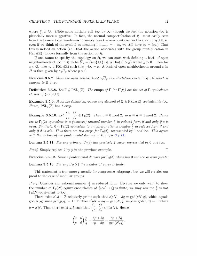
CHAPTER 3. THE POINCARÉ UPPER HALF-PLANE 42
where pq ∈ Q. (Note some authors call i∞ by ∞, though we feel the notation i∞ is
pictorially more suggestive. In fact, the natural compactifcation of H—most easily seenfrom the Poincaré disc model—is to simply take the one-point compactification of H∪R, soeven if we think of the symbol ∞ meaning limx→∞ = +∞, we still have ∞ = i∞.) Thatthis is indeed an action (i.e., that the action associates with the group multiplication inPSL2(Z)) follows formally from the action on H.
If one wants to specify the topology on H, we can start with defining a basis of openneighborhoods of i∞ in H to be Uy = i∞ ∪ z ∈ H : Im(z) > y where y > 0. Then forx ∈ Q, take γx ∈ PSL2(Z) such that γi∞ = x. A basis of open neighborhoods around x inH is then given by γxUy where y > 0.
Exercise 3.5.7. Show the open neighborhood γxUy is a Euclidean circle in H ∪ R which istangent to R at x.
Definition 3.5.8. Let Γ ⊆ PSL2(Z). The cusps of Γ (or Γ\H) are the set of Γ-equivalenceclasses of i∞ ∪Q.
Example 3.5.9. From the definition, we see any element of Q is PSL2(Z)-equivalent to i∞.Hence, PSL2(Z) has 1 cusp.
Example 3.5.10. Let(a bc d
)∈ Γ0(2). Then c ≡ 0 mod 2, so a ≡ d ≡ 1 mod 2. Hence
i∞ is Γ0(2) equivalent to a (nonzero) rational number ac in reduced form if and only if c is
even. Similarly, 0 is Γ0(2) equivalent to a nonzero rational number bd in reduced form if and
only if d is odd. Thus there are two cusps for Γ0(2), represented by 0 and i∞. This agreeswith the picture of the fundamental domain in Example 3.4.11.
Lemma 3.5.11. For any prime p, Γ0(p) has precisely 2 cusps, represented by 0 and i∞.
Proof. Simply replace 2 by p in the previous example.
Exercise 3.5.12. Draw a fundamental domain for Γ0(3) which has 0 and i∞ as limit points.
Lemma 3.5.13. For any Γ0(N) the number of cusps is finite.
This statement is true more generally for congruence subgroups, but we will restrict ourproof to the case of modular groups.
Proof. Consider any rational number pq in reduced form. Because we only want to show
the number of Γ0(N)-equivalence classes of i∞ ∪ Q is finite, we may assume pq is not
Γ0(N)-equivalent to i∞.There exist c′, d ∈ Z relatively prime such that c′pN + dq = gcd(pN, q), which equals
gcd(N, q) since gcd(p, q) = 1. Further c′pN + dq = gcd(N, q) implies gcd(c, d) = 1 where
c = c′N . Thus there exist a, b such that(a bc d
)∈ Γ0(N). Hence
(a bc d
)p
q=ap+ bq
cp+ dq=
ap+ bq
gcd(N, q).

CHAPTER 3. THE POINCARÉ UPPER HALF-PLANE 43
Therefore replacing pq by something Γ0(N)-equivalent, we may assume q|N .
Further, since T ∈ Γ0(N), we see
T bp
q=
(1 b0 1
)p
q=p+ bq
q
is also Γ0(N)-equivalent to pq . Hence we can also assume 0 ≤ p < q. This gives only a finite
number of possible non-equivalent pq .
One can refine the argument above to precisely count the number of cusps for Γ0(N).
Exercise 3.5.14. Show that the number of cusps for Γ0(N) is given by∑d|N
φ(gcd(d,N/d))
where φ is the Euler phi function.
*Exercise 3.5.15. Compute the cusps for Γ0(4).

Chapter 4
Modular Forms
4.1 Modular curves and functions
Definition 4.1.1. The modular curves of level N , Y0(N) and X0(N), are defined to be
Y0(N) = Γ0(N)\H
andX0(N) = Γ0(N)\H.
In particular, Y0(1) = PSL2(Z)\H and X0(1) = PSL2(Z)\H.Note X0(N) is the compactification of Y0(N) obtained by adding the cusps for Γ0(N),
as described in the last chapter.
Exercise 4.1.2. Show X0(N), with the quotient topology, is compact, using the topology onH described Section 3.5.
Before we go further, let us explain the terminology a bit. In Section 2.5, we saw thatY0(1) parameterized lattices in C, equivalently, isomorphism classes of (generalized) ellipticcurves. (Some lattices would give a curve with discriminant 0, and these degenerate curvesare called generalized elliptic curves). One can also define a generalized elliptic curve forthe cusp in X0(1), and thus view X0(1) as parametrizing the space of (generalized) ellipticcurves over C, up to analytic isomorphism. Similarly, X0(N) parametrizes isomorphismclasses of pairs (E,C) where E is a (generalized) elliptic curve over C and C is a cyclicsubgroup of order N .
In algebraic geometry, a moduli space is a geometric object (curve, surface, manifold,etc.) whose points parametrize a class of other geometric objects, in this case elliptic curveswith a distinguished cyclic subgroup. The Riemann surface X0(N) can also be viewed as analgebraic curve over C, hence the term modular curve. Realizing X0(N) as a moduli spaceis fundamental in the theory of elliptic curves, though we will not focus on this aspect inthis course.
For those familiar with Riemann surfaces, or complex manifolds, we can state the defi-nition of a modular function very simply.
44

CHAPTER 4. MODULAR FORMS 45
Definition 4.1.3. (Riemann surface version) A modular function of level N is a mero-morphic function f : X0(N)→ C.
For both readers familiar with Riemann surfaces and those not, let us translate this intoa statement about functions on H.
First, think about f restricted to Y0(N) = Γ0(N)\H. Being a meromorphic function onY0(N) means we can lift f to a function f : H→ C such that
(i) f(γz) = f(z) for all γ ∈ Γ0(N), and(ii) f is meromorphic on H.
Now we need to explain what it means for f to be meromorphic at the cusps of X0(N).We first consider the notion of meromorphy at the cusp i∞. It may be helpful at this pointto recall the discussion at the end of Section 2.3 (though our notation here is different—fand F instead of g and G, and q instead of ζ).
Since T =
(1 10 1
)∈ Γ0(N), we know f(Tz) = f(z + 1) = f(z), i.e., f is periodic of
period 1. Consequently, this means f(z) has a Fourier expansion
f(z) =∑n∈Z
ane2πinz
where the n-th Fourier coefficient an is given by
an =
∫ 1
0f(z)e−2πinzdx, (z = x+ iy)
valid for all z ∈ H. (Our argument at the end of Section 2.3 will justify that an does notdepend upon y.) Put q = e2πiz. Thus the Fourier expansion becomes
f(z) =∑n∈Z
anqn. (4.1.1)
This is also called the q-expansion for f . Note that the map z = x+ iy 7→ q = e−2πye2πix isan analytic bijection from the vertical strip
z ∈ H : −1
2 ≤ Im(z) < 12
in H to the punctured
discD× = z ∈ C : 0 < |z| < 1. Therefore we may think of f(z), a priori a periodic functionon H, instead as a function F (q) on D×.
If z = iy, then q = e−2πy, so as z → i∞, q → 0. Hence f(z) being meromorphic at thecusp z = i∞ precisely means that F (q) is meromorphic at q = 0. If F (q) is meromorphicat q = 0, then it has a Laurent expansion, which must equal the Fourier expansion (4.1.1).In other words F (q) is meromorphic at q = 0 if and only if the Fourier coefficients an of fare independent of y and
(iii-a) the Fourier coefficients an for all but finitely many n < 0.
By (2.3.1), this is equivalent to the condition that |f(z)| grows at most exponentially asy →∞, i.e.,
(iii-a’) for y 0, there exists m such that |f(z)| < emy.
CHAPTER 4. MODULAR FORMS 46
Now that we know what it means for f(z) to be meromorphic at the cusp i∞, we canuse this to say what it means to be meromorphic at any cusp. Namely consider a cusp forΓ0(N) represented by z0 ∈ Q, and let τ ∈ PSL2(Z) be an element which maps i∞ to z0.Consider the function
f |τ (z) = f(τz).
Since τ is an isometry of H, f |τ is also meromorphic on H. Thus we can view |τ as anoperator on meromorphic functions of H, called the slash operator .
Lemma 4.1.4. Suppose f(γz) = f(z) for γ ∈ Γ0(N). Let τ ∈ PSL2(Z). Then f |τ (z+N) =f |τ (z) for all z ∈ H.
Proof. First note that f |τ is left-invariant under τ−1Γ0(N)τ : for γ ∈ Γ0(N), we have
f |τ (τ−1γτz) = f(γτz) = f(τz) = f |τ (z).
On the other hand, note that the principal congruence subgroup
Γ(N) = γ ∈ PSL2(Z) : γ ≡ I mod N ⊆ Γ0(N)
is a normal subgroup of PSL2(Z). In particular Γ(N) ⊆ τ−1Γ0(N)τ , so f |τ is invariantunder TN ∈ Γ(N). This proves the claim.
This lemma means that f |τ is also periodic with period N . (It may actually have smallerperiod if a smaller power of T lies in τ−1Γ0(N)τ .) Consequently, f |τ has a Fourier expansionof the form
f |τ (z) =∑n∈Z
aτ,nqnN , (4.1.2)
whereqN = e2πiz/N .
(If, for instance, f |τ actually has period 1, we can write f |τ (z) =∑cnq
n, i.e., the aτ,n = 0unless N |n.) What f(z) to be meromorphic at the cusp z0 means is precisely that f |τ ismeromorphic at i∞. Now our discussion about what it meant for f(z) to be meromorphicat i∞ goes through for functions with period N just as well, and we see f(z) is meromorphicat the cusp z0 if and only if
(iii-b) the Fourier coefficients aτ,n = 0 for all but finitely many n < 0;
or equivalently,
(iii-b’) for y 0, there exists m such that |f |τ (z)| < emy.
Observe that (4.1.2) can be used to give another series expansion for f . Namely, sincef(z) = f |τ (τ−1z), we can write
f(z) =∑n∈Z
aτ,nqnτ , qτ = e2πiτ−1z/N . (4.1.3)
This expansion, again valid for all z ∈ H, is called a Fourier (or q−) expansion at z0
(with respect to τ) for f(z). Consequently, we sometimes refer to the usual Fourier expansion(4.1.1) as the Fourier expansion at i∞.

CHAPTER 4. MODULAR FORMS 47
A priori, the Fourier expansion (4.1.3) at z0, and consequently the conditions (iii-b) and(iii-b’), depend upon the choice of τ ∈ PSL2(Z) we used to send i∞ to z0. We would like tosay all of these are independent of the choice of τ—and in fact the choice of z0 representingthe given cusp—and this is essentially what the following lemma tells us.
Lemma 4.1.5. Suppose a meromorphic f : H→ C satisfies f(γz) = f(z) for all γ ∈ Γ0(N).Let z0, z
′0 ∈ i∞∪Q represent the same cusp for Γ0(N), i.e., z′0 = γz0 for some γ ∈ Γ0(N).
Now suppose τ, τ ′ ∈ PSL2(Z) such that τ ·i∞ = z0 and τ ′ ·i∞ = z′0. Then f |τ (z) = f |τ ′(z+j)for some j ∈ Z.
Consequently, the Fourier coefficients with respect to τ and τ ′ are related by
aτ ′,n = aτ,ne2πij/N
for all n; in particular |aτ ′,n| = |aτ,n| for all n.
Proof. First observe that γτ is an element of PSL2(Z) which sends i∞ to z′0. Therefore
(τ ′)−1γτ =
(a bc d
)∈ PSL2(Z)
which preserves i∞. By the definition of our action of PSL2(Z) on i∞ ∪ Q, this meansc = 0, whence a = c = ±1 so (τ ′)−1γτ = T j for some j ∈ Z, i.e., τ ′ = γτT−j . Consequently
f |τ ′(z) = f(τ ′z) = f(γτT−jz) = f(τT−jz) = f |τ (T−jz) = f |τ (z − j).
This gives the first part of the lemma.Since we may also the last equation as f |τ ′ = f |τT−j , the Fourier expansion at z′0 (w.r.t.
τ ′) for f(γz) is
f(z) = f(γz) =∑n∈Z
aτ ′,ne2πiT jτ−1γ−1γz/N =
∑n∈Z
aτ ′,ne2πiT jτ−1z/N =
∑n∈Z
aτ ′,ne2πij/Ne2πiτ−1z/N .
Comparing this with the Fourier expansion at z0 (w.r.t. τ) for f(z) gives the second assertion.
In other words, f(z) may technically have more than one Fourier expansion at a givencusp, but any Fourier expansion is obtained from a given one by replacing the parameterqτ = e2πiz/N with a parameter of the form qγτT−j = e2πi(τγ−1z+j) for j ∈ Z and γ ∈ Γ0(N)
and multiplying all the Fourier coefficients aτ,n by a fixed root of unity e2πij/N .
Now we can recast Definition 4.1.3 in the language it is typically presented in mostmodular forms texts.
Definition 4.1.6. (Upper half-plane version) We say a function f : H→ C is a modularfunction of level N if
(i) f(γz) = f(z) for all γ ∈ Γ0(N);(ii) f is meromorphic on H; and(iii) f is meromorphic at each cusp of Γ0(N); i.e., for each τ ∈ PSL2(Z), the Fourier
coefficients aτ,n as defined in (4.1.3) satisfy aτ,n = 0 for all but finitely many n < 0.
CHAPTER 4. MODULAR FORMS 48
In practice one only needs to check the condition on negative Fourier coefficients aτ,n asτ ranges over a finite set of elements of PSL2(Z) such that τ ∈ i∞ runs over all cusps ofΓ0(N). Further, our discussion above of course implies that (iii) is equivalent to
(iii’) for each τ ∈ PSL2(Z), the function f |τ is of moderate growth in y = Im(z), i.e.,for y large, there exists m such that |f |τ (z)| < emy.
Exercise 4.1.7. Suppose f is a modular function of level 1 with Fourier expansion f(z) =∑∞−m anq
n. Show that for any τ ∈ PSL2(Z), the Fourier coefficients with respect to τ arethe usual Fourier coefficients, i.e., aτ,n = an for all n.
Note that our above discussion goes through if we replace Γ0(N) by an arbitrary con-gruence subgroup Γ, as Γ ⊇ Γ(N) for some N . Thus for any congruence subgroup Γ ofPSL2(Z), we can say f : H → C is a modular function for Γ by simply replacing Γ0(N)by Γ in the definition above.
Exercise 4.1.8. Suppose f is a modular function for a congruence subgroup Γ(N).(i) For τ ∈ PSL2(Z), show f |τ is a modular function for τ−1Γ(N)τ .(ii) Deduce that |τ : f 7→ f |τ operates on the space of modular functions for Γ(N).(iiii) Show f |τ = f |τ ′ if τ ′ ∈ Γτ . Hence at most |Γ(N)\PSL2(Z)| of the operators |τ can
be distinct.(iv) Show (f |τ )|τ ′ = |ττ ′ , hence these operators give a right action of the quotient group
Γ(N)\PSL2(Z) on the space of modular functions for Γ(N).
There are a couple obvious things we can say now about modular functions.
Example 4.1.9. Any constant function on H is a modular function for any congruencesubgroup Γ.
Example 4.1.10. Suppose Γ, Γ′ are two congruence subgroups such that Γ′ ⊆ Γ. If f is amodular function for Γ, then f is a modular function for Γ′. In particular, if f is a modularfunction of level N and N |M , then f is also a modular function of level M .
Now of course we would like to know if some interesting (non-constant) modular functionsexist. It turns out they are not trivial to construct. For example, let us try to naivelyconstruct a modular function for PSL2(Z), i.e., a modular function of level 1. Let g(z) = 1
zn
for n ∈ Z. Then we can try to average over the PSL2(Z)-translates
f(z) =∑
γ∈PSL2(Z)
g(γz) =1
(γz)n.
We can see this diverges just by considering γ of the form ST j . Such γ contribute∑j∈Z
1
(ST jz)n=∑ 1
(S(z + j))n=∑ 1
(−1/(z + j))n=∑j
(−1)n(z + j)
to the average, but this already diverges.An alternative approach might be the following. Since PSL2(Z) is generated by S (z 7→
−1/z) and T (z 7→ z+ 1), we just need to find a function invariant under both of them. We
CHAPTER 4. MODULAR FORMS 49
know e2πiz is invariant under T , so we could average this over the group 〈S〉 = I, S. Thiswould give us
e2πiz + e2πiSz = e2πiz + e−2πi/z.
Unfortunately, because of the second term, this is no longer invariant under T . (And if onetries to average over enough of PSL2(Z) to make the sum formally PSL2(Z)-invariant, thenit will diverge as in the first attempt.)
The easiest way to construct nontrivial modular functions will be to use modular forms.We will discuss this in the next section. First, we will present one result about nontrivialmodular functions—they cannot be holomorphic!
Recall the following result of complex analysis.
Theorem 4.1.11. (Open Mapping Theorem) Let U ⊆ C be an open set, and f : U → Cbe holomorphic and nonconstant. Then f is an open map, i.e., f maps open sets to opensets.
Corollary 4.1.12. Let X be a compact Riemann surface, and f : X → C holomorphic.Then f is constant.
Proof. What f : X → C holomorphic means is the following. Around any point p ∈ X,there is an open set U such that there is an analytic isomorphism ιU → D with the openunit disc D ⊆ C. For each such p, the map f ι−1 : D → C is holomorphic at p.
Consequently, the Open Mapping Theorem says if f is not constant, f(X) is an opensubset of C. However, since f is continuous and X is compact, f(X) is also compact. Butthere are no open compact subsets of C.
Since X0(N) is compact (as is Γ\H for any congruence subgroup Γ), there are no non-constant holomorphic modular functions of level N (or for any congruence subgroup Γ).In fact, since the torus C/Λ is also a compact Riemann surface for a lattice Λ, the abovecorollary also tells us there are no nonconstant holomorphic elliptic functions with respectto Λ.
4.2 Eisenstein series
Even though we couldn’t construct modular functions by an averaging process like we couldfor elliptic functions, the theory of elliptic functions does provide a subtle hint for construct-ing modular functions. Recall that for a lattice Λ ⊂ C, the field of elliptic functions withrespect to Λ was generate by the associate ℘-function and its derivative ℘′. We constructed℘′ by an simple averaging technique, but the construction of ℘ was more complicated.
Consequently, one might ask if the derivatives of modular functions are simpler to con-struct than modular functions themselves. Suppose f is a modular function for Γ. Let γ ∈ Γ
and write γ =
(a bc d
). Then
d
dzf(z) =
d
dzf(γz) = f ′(γz) · d
dz(γz) = f ′(γz) · d
dz
az + b
cz + d=
1
(cz + d)2f ′(γz).
CHAPTER 4. MODULAR FORMS 50
In other words, f ′ is no longer exactly invariant by Γ, but satisfies the transformation law
f ′(γz) = (cz + d)2f ′(z).
Similarly if g(z) = f (k)(z), we have
g(γz) = (cz + d)2kg(z).
As I have suggested, it is easier to construct functions with these transformation propertiesthan those which are strictly invariant under some Γ.
Definition 4.2.1. Let f : H→ C be meromorphic and Γ a congruence subgroup of PSL2(Z).Let k ∈ 2N ∪ 0. If
f(γz) = (cz + d)kf(z), γ =
(a bc d
)∈ Γ, z ∈ H,
then f is weakly modular (or a weak modular form) of weight k for Γ. If Γ = Γ0(N)we say f is weakly modular of weight k and level N .
Note the factor cz + d is not quite determined uniquely by a(a bc d
)∈ PSL2(Z), but
only up to ±1. However since k is assumed to be even, this creates no ambiguity in thedefinition above.
The adjective “weak” here refers to the fact that there is no condition at the cusps, likewe had for modular functions.
(One can define weak modular forms, and modular forms, of odd weight k, just byreplacing PSL2(Z) with SL2(Z). However for the same reason, they will not exist unlessΓ ⊆ SL2(Z) is a sufficiently small congruence subgroup such that γ ∈ Γ =⇒ −γ 6∈ Γ, orequivalently −I 6∈ Γ. This rules out the case of modular groups Γ0(N) viewed as subgroupsof SL2(Z), but not Γ1(N) or Γ(N). Since our main focus in this course is modular forms forΓ0(N), we will not have much reason to consider these forms of odd weight.)
Lemma 4.2.2. Suppose f (resp. g) is weakly modular of weight k (resp. l) for Γ.(i) If k = l and c ∈ C, then cf +g is weakly modular of weight k = l for Γ. Hence weakly
modular functions of weight k form a complex vector space.(ii) f · g is weakly modular of weight k + l for Γ.(iii) f
g is weakly modular of weight k − l for Γ provided g 6≡ 0.
The proof is immediate.
Consequently, if we can construct two different weak modular forms of weight k for somek, then their quotient will be a nontrivial weak modular form of weight 0, which is a modularfunction provided the condition of meromorphic at the cusps is satisfied. We will come backto the condition at the cusps later, and use this to define meromorphic and holomorphicmodular forms. For now, we will show how to construct weak modular forms of even weightk > 2.
CHAPTER 4. MODULAR FORMS 51
The idea is basically to take a weighted average of some function g(z) : H → C overa congruence subgroup Γ. To explain this, for γ ∈ PSL2(Z), we define the automorphyfactor j(γ, z) : PSL2(Z)× H→ C to be
j(γ, z) = cz + d, γ =
(a bc d
). (4.2.1)
(As we remarked after Definition 4.2.1, j(γ, z) is only defined up to ±1, but as we will raisethis to an even power, this causes no ambiguity.) For k even, consider the average
f(z) =∑γ∈Γ
1
(cz + d)kg(γz) =
∑γ∈Γ
j(γ, z)−kg(γz).
Then we formally havef(γ0z) =
∑γ∈Γ
j(γ, γ0z)−kg(γγ0z).
Now we will need the following property of the automorphy factor.
Lemma 4.2.3. For γ, γ′ ∈ PSL2(Z), we have
j(γγ′, z) = ±j(γ′, z)j(γ, γ′z).
Proof. Observe that (3.2.1) implies
Im(γz) =Im(z)
|j(γ, z)|2.
HenceIm(z)
|j(γγ′, z)|2= Im(γγ′z) =
Im(γ′z)
|j(γ, γ′z)|2=
Im(z)
|j(γ, γ′z)j(γ′, z)|2.
This shows the lemma is true up to taking absolute values.Thus the lemma follows from the following claim: Suppose f and g are meromorphic
functions with |f(z)|2 = |g(z)|2. Then f(z) = ζg(z) where |ζ| = 1. We may assume g 6≡ 0.The hypothesis just says ff = gg, i.e., f/g = g/f . Hence the image of the meromorphicfunction f/g is contained in the set of z ∈ C such that z = 1/z, i.e., |z|2 = 1. By the OpenMapping Theorem (restrict to an open set where f/g is holomorphic), this is impossibleunless f/g is constant. Then the absolute value condition implies f(z) = ζg(z) where|ζ| = 1.
This meansj(γγ′, z) = ζj(γ′, z)j(γ, γ′z)
with |ζ = 1|. Then the fact that j(γ, z) is of the form cz + d where c, d ∈ Z (so e.g.,j(γ, z) ∈ Z for z ∈ Z) implies that ζ = ±1.
By this lemma, we have
f(γ0z) = j(γ0, z)k∑γ∈Γ
j(γγ0, z)−kg(γγ0z) = j(γ0, z)
k∑γ∈Γ
j(γ, z)−kg(γz) = j(γ0, z)kf(z),
CHAPTER 4. MODULAR FORMS 52
where we replaced γ by γγ−10 in the middle step. In other words, provided f(z) converges
and is meromorphic, f(z) is weakly modular of weight k.However, as alluded to in the last section, averaging over all of Γ will be too much for
f(z) to converge. We also briefly toyed with a second idea—start with a periodic functionand average over just what we need to yield the weak modularity condition for Γ. Let’srestrict to the case Γ = Γ0(N) so T ∈ Γ. (Arbitrary Γ ⊇ Γ(N) can be treated similarlysince TN ∈ Γ(N).) Let P be the subgroup of PSL2(Z) generated by T , i.e.,
P = 〈T 〉 =
(1 n0 1
): n ∈ Z
⊆ Γ0(N).
Note for γ ∈ P , j(γ, z) = 1, so any periodic function g(z) with period 1 satisfies the weakmodularity condition for T . Thus averaging over P\Γ0(N) should, at least formally, yieldsomething which is weakly modular.
First let’s describe this coset space.
Lemma 4.2.4. A complete set of representatives for P\Γ0(N) is parametrized by the set(c, d) ∈ Z2 : c ≡ 0 mod N, gcd(c, d) = 1
/± 1,
where a coset representative with parameter (c, d) can be taken uniquely in the form(a bc d
)∈
Γ0(N) with 0 ≤ b < |d|, or(a bc d
)= S if (c, d) = ±(1, 0) and N = 1.
Proof. Let γ =
(a bc d
)∈ Γ0(N), so ad− bc = 1 and c ≡ 0 mod N . We can replace γ with
the element (1 n0 1
)(a bc d
)=
(a+ cn b+ dnc d
)which lies in the same right P -coset of Γ0(N) as γ. First suppose d = 0. Then −bc = 1so we may assume b = −c = 1, which can only happen if N = 1. Choosing n = −a shows
γ ∈ P(
0 1−1 0
).
Now suppose d 6= 0. Then we may (uniquely) choose n such that 0 ≤ b + dn < |d|.Consequently we may assume 0 ≤ b < |d|. On the other hand, the determinant conditionsays a = 1+bc
d ∈ Z, i.e., bc ≡ −1 mod d. This determines b, and consequently a, uniquely.
So one idea might be to average the function e2πiz over this coset space, but again thereare some issues with convergence. However, there’s a simpler periodic function we coulduse—a constant function! In the k = 0 case, this obviously diverges, but if k ≥ 4, it willconverge.
Definition 4.2.5. Let k ≥ 4 be even. The (normalized) Eisenstein series of weight kand level N is defined to be
Ek,N (z) =∑
γ∈P\Γ0(N)
j(γ, z)−k =1
2
∑(c,d)∈Z2
gcd(c,d)=1c≡0 mod N
1
(cz + d)k. (4.2.2)

CHAPTER 4. MODULAR FORMS 53
If N = 1 we often write Ek for Ek,N .
Note the second expression for Ek,N in the definition follows (formally) from the abovelemma, and the factor of 1
2 comes from the fact that we include both (c, d) and (−c,−d) inthe sum.
Proposition 4.2.6. The Eisenstein series Ek,N converges absolutely and uniformly on com-pact subsets of H. Therefore, Ek,N is a weak modular form of weight k and level N which isholomorphic on H.
Proof. The discussion above shows that Ek,N transforms formally under Γ0(N) as it should.Specifically, for γ0 ∈ Γ0(N), we have
Ek,N (γ0z) =∑
γ∈P\Γ0(N)
j(γ, γ0z)−k = j(γ0, z)
k∑
γ∈P\Γ0(N)
j(γγ0, z)−k.
Since right multiplying P\Γ0(N) by γ−10 simply permutes the cosets P\Γ0(N), we may
replace γ by γγ−10 in the sum to see
Ek,N (γ0z) = j(γ0, z)kEk,N (z). (4.2.3)
Now let’s deal with convergence. Since the series Ek,N for N > 1 is a sum over a strictlysmaller set of terms than the series for Ek = Ek,1, it suffices to prove absolute convergencefor Ek(z).
First suppose z lies in the standard fundamental domain F for PSL2(Z). Then
|cz + d|2 = (cz + d)(cz + d) = c2|z|2 + 2cdRe(z) + d2.
Since z ∈ F , |z| ≥ 1 and Re(z) ≤ 12 so
|cz + d|2 ≥ c2 − |cd|+ d2 =
|cζ3 + d|2 cd > 0
|cζ3 − d|2 cd < 0.
Hence for z ∈ F ,
|Ek(z)| ≤∑c,d≥0
gcd(c,d)=1
1
|cζ3 + d|k+
∑c≥0, d≤0
gcd(c,d)=1
1
|cζ3 − d|k= 2
∑c,d≥0
gcd(c,d)=1
1
|cζ3 + d|k.
Note that cζ3 + d : c, d ∈ Z form the lattice in C generated by 1 and ζ3. Now we wantto solve the lattice point problem of estimating how many (c, d) ∈ Z2 there are such thatcζ3 +d lies inside the open disc Dr of radius r centered at the origin, i.e., bound the numberof (c, d) such that
|cζ3 + d| < r.
Observe that if |c| ≥ 2r, then |Im(cζ3 + d)| = |Im(cζ3)| = |c|√
32 > r, i.e., cζ3 + d 6∈ Dr.
Similarly, looking at real parts show if |c| < 2r then we must have |d| < 2r if cζ3 + d ∈ Dr.

CHAPTER 4. MODULAR FORMS 54
I.e., the number of (c, d) such that |cζ3 + d| ∈ Dr is at most 4r2. In particular, the numberof (c, d) such that |cζ3 + d| ∈ Dr+1 −Dr is at most 4(r + 1)2, and we can bound
|Ek(z)| ≤∑
(c,d)∈Z2
(c,d)6=(0,0)
1
|cζ3 + d|k≤
∑(c,d)∈Z2
r≤|cζ3+d|<r+1
1
rk≤∞∑r=1
4(r + 1)2
rk,
which converges for k > 3. This establishes absolute convergence on F .Then the formal identity (4.2.3) implies we have absolute convergence at any point in H.
Namely we can write any point of H as γz for some γ ∈ PSL2(Z) and z ∈ F . Thus (4.2.3)says |Ek(γz)| = |j(γ, z)kEk(z)|.
Since the bound above in F is independent of z, i.e., Ek(z) is a bounded function onF , it also implies uniform convergence of Ek(z) and Ek,N (z) on F . For Ek(z) this impliesuniform convergence on compact sets of H by the transformation property of Ek(z) sincefor a fixed γ, j(γ, z) is uniformly bounded on compact sets. Because the tail of a seriesfor Ek,N (z) can be bounded by the tail of a series for Ek(z), this also implies Ek,N (z) isuniformly bounded on compact subsets.
The theory of normal families or normal convergence in complex analysis says that ifa series of analytic functions converges absolutely and uniformly on compact subsets, thelimit function is also analytic. This finishes the proposition.
For the future, let us record one more thing we got out of the above proof.
Corollary 4.2.7. Ek,N (z) is bounded on the standard fundamental domain for PSL2(Z).In particular, Ek,N (z) is bounded as z → i∞.
Proof. The first statement comes directly from the proof. On the other hand, if Imz > 1,then T jz ∈ F for some j. Therefore Ek,N (z) = j(T j , z)−kEk,N (T jz) = Ek,N (T jz) is alsobounded.
This says Ek(z) (as well as Ek,N (z)) should be “holomorphic at i∞.” Once we defineholomorphy at the cusps in the next section, we will see these Eisenstein series are holomor-phic at all cusps, making them holomorphic modular forms.
One interesting and elementary aspect of Eisenstein series is their Fourier expansion.Since Ek,N (z + 1) = Ek,N (z), it has a Fourier expansion
Ek,N (z) =∞∑n=0
anqn, q = e2πiz.
Here the sum starts from n = 0 since Ek,N (z) is holomorphic at i∞. The idea is to use thefollowing.
Lemma 4.2.8. (Lipschitz’ formula) Let k ≥ 2 and z ∈ H. Then∑n∈Z
1
(z + n)k= Ck
∞∑n=1
nk−1qn
where
Ck =(−2πi)k
(k − 1)!.

CHAPTER 4. MODULAR FORMS 55
Proof. Recall the product formula for sine:
sinπz = πz
∞∏n=1
(1− z2
n2
).
Taking the logarithmic derivative of this gives
π cotπz =1
z+∞∑n=1
(1
z + n+
1
z − n
). (4.2.4)
(Writing the cotangent formula this way as opposed to∑
n∈Z1
z+n gives a series whichis absolutely convergent.) On the other hand, since sin(πz) = Im(πz) = eπiz−e−πiz
2i andcos(πz) = Re(πz) = eπiz+e−πiz
2 , we have
π cotπz = πieπiz + e−πiz
eπiz − e−πiz= πi
e2πiz + 1
e2πiz − 1= πi
q + 1
q − 1= πi− 2πi
1− q= πi− 2πi
∞∑n=0
qn.
Taking the (k−1)-st derivative of each of these expressions for π cotπz gives the lemma.
Comparing
Ek,N (z) =1
2
∑(c,d)∈Z2
gcd(c,d)=1c≡0 mod N
1
(cz + d)k
with Lipschitz’ formula, it would appear easier to compute the Fourier expansion for Ek,N (z)without the condition that gcd(c, d) = 1 in the above sum.
For simplicity, let’s first consider the case of full level, i.e., N = 1. Define
Gk(z) =∑
(0,0)6=(c,d)∈Z2
1
(cz + d)k(4.2.5)
=∞∑n=1
∑(c,d)∈Z2
gcd(c,d)=n
1
(cz + d)k
=
∞∑n=1
1
nk
∑(c,d)∈Z2
gcd(c,d)=1
1
(cz + d)k= 2ζ(k)Ek(z),
where ζ(s) =∑ 1
ns for Re(s) > 1 is the Riemann zeta function. Since Gk(z) is just a scalarmultiple of Ek(z), we also call Gk(z) an (unnormalized) Eisenstein series. (In fact, in mostclassical treatments, one defines Gk(z) before Ek(z).)

CHAPTER 4. MODULAR FORMS 56
Now applying the Lipschitz formula, we have
Gk(z) =∑
(0,0) 6=(c,d)∈Z2
1
(cz + d)k
=∑d 6=0
1
dk+ 2
∞∑c=1
∑d∈Z
1
(cz + d)k
= 2ζ(k) + 2Ck
∞∑c=1
∞∑n=1
nk−1e2πiczn
= 2ζ(k) + 2Ck
∞∑c=1
∞∑n=1
nk−1qcn.
Then what is the coefficient of a given qm? There is a contribution from nk−1qcn whenevercn = m, hence it is 2Ckσk−1(m) where σk(m) is the classical divisor function
σk(m) =∑d|m
dk.
This establishes the following Fourier expansion.
Proposition 4.2.9. Let k ≥ 4 be even. Then we have the following Fourier expansion forthe Eisenstein series of weight k.
Gk(z) = 2ζ(k) + 2Ck
∞∑n=1
σk−1(n)qn.
In terms of the normalized Eisenstein series, we can write this as
Ek(z) = 1− 2k
Bk
∞∑n=1
σk−1(n)qn,
where Bk is the k-th Bernoulli number.
We recall the Bernoulli numbers can be defined as the coefficients in the expansion
x
ex − 1=∞∑k=0
Bkxk
k!.
Alternatively we can define them recursively by B0 = 1 and
Bk = −k−1∑j=0
(kj
)Bj
k − j + 1.
Exercise 4.2.10. Check these two definitions of Bk are equivalent.
CHAPTER 4. MODULAR FORMS 57
Proof. We already derived the expansion for Gk(z). Dividing by 2ζ(k) and using Euler’sformula
ζ(k) = −CkBk2k
gives the expansion for Ek(z).
The fact that the Fourier coefficients of Eisenstein series are divisor functions—objectsof study in elementary number theory—is our first real evidence that modular forms andfunctions are important in number theory. Later, we can use the theory of modular forms toprove results about these divisor functions, as well as relate them to problems in quadraticforms, as we discussed in the introduction.
At this point we can say why the Ek are called normalized Eisenstein series—they arenormalized so that their leading Fourier coefficient is 1.1 Since z = i∞ corresponds to q = 0,the 0-th Fourier coefficient gives us the “value” of a periodic function at i∞, i.e., Ek(i∞) = 1.
Example 4.2.11.
E4(z) = 1 + 240
∞∑n=1
σ3(n)qn.
E6(z) = 1− 504∞∑n=1
σ5(n)qn.
E8(z) = 1 + 480∞∑n=1
σ7(n)qn.
Exercise 4.2.12. From the first few examples, it looks like the Fourier coefficients for Ekmight always be integers. This is not true (though they are clearly rational from Proposition4.2.9). Find the first even k such that 2k
Bk6∈ Z.
To come back to the original question we asked as motivation—are derivatives of mod-ular functions easier to construct directly than modular functions themselves?—we’ve onlyconstructed holomorphic things which behave like derivatives of modular functions. Sincenon-constant modular functions are non-holomorphic, their derivatives are non-holomorphicand cannot be things like these Eisenstein series. However, we can still use these Eisensteinseries (or more generally holomorphic modular forms, which we define below) to constructmodular forms by taking quotients! (Of course, all this was just motivation for the funnytransformation law in the definition of weak modular forms—we’re really interested in mod-ular forms in this course, not modular functions.) Here is an example that is important inthe theory of elliptic curves.
*Exercise 4.2.13. We define the j-invariant to be
j(z) = 1728E4(z)3
E4(z)3 − E6(z)2.
Use the Fourier expansions for Ek to show j is a nonconstant modular function for PSL2(Z).1One can instead normalize so that a1 = 1. This will have the benefit that the n-th Fourier coefficient is
just σk−1(n), so the an’s with n ≥ 1 are multiplicative. We will consider this other normalization in (6.0.1)and again in Chapter 8.
CHAPTER 4. MODULAR FORMS 58
Since isomorphism classes of (generalized) elliptic curves are parametrized by X0(1) =PSL2(Z)\H, this gives a (nontrivial) invariant for elliptic curves which varies smoothly inthe parameters defining the curve.
Remark. While it is obvious that Ek cannot converge if k = 0, it is natural to ask whathappens if k = 2. The sum does not converge absolutely, but if we specify the order ofsummation, we can get a convergent function.
Exercise 4.2.14. Define
E2(z) =1
2ζ(2)
∞∑c=−∞
( ∞∑′
d=−∞
1
(cz + d)2
),
where the prime on the inner sum means we omit the term d = 0 when c = 0.(a) Using Lipshitz’ formula on the inner sum first, show the resulting expression for
E2(z) converges absolutely.(b) Show
E2(z) = 1− 24∞∑n=1
σ1(n)qn.
However E2(z) is not quite modular. It can be shown (e.g., [Kob93, p. 113]) that
E2(−1/z) = z2E2(z) +12
2πiz.
Now let us consider the case of higher level. The naive generalization to level N wouldbe to consider
Gk,N (z) =∑
(0,0)6=(c,d)∈Z2
c≡0 mod N
1
(cz + d)k=∞∑n=1
∑(c,d)∈Z2
c≡0 mod Ngcd(c,d)=n
1
(cz + d)k, (4.2.6)
but we can’t write this in terms of Ek,N (z) as simply as we did when N = 1. The reasonis that if we rewrite the inner sum on the right as gcd(c, d) = 1 and factor out a n−k, webreak the condition c ≡ 0 mod N if gcd(n,N) 6= 1.
Let’s see what happens when N = p is prime. Then
Gk,p(z) =∑
(0,0)6=(c,d)∈Z2
c≡0 mod p
1
(cz + d)k
=∑
(c,d)∈Z2
c≡0 mod pgcd(d,p)=1
1
(cz + d)k+
∑(0,0) 6=(c,d)∈Z2
c≡d≡0 mod p
1
(cz + d)k
= G∗k,p(z) +1
pkGk(z),
CHAPTER 4. MODULAR FORMS 59
where
G∗k,p(z) =∑
(c,d)∈Z2
c≡0 mod pgcd(d,p)=1
1
(cz + d)k
=∑n>0
gcd(n,p)=1
∑(c,d)∈Z2
c≡0 mod pgcd(c,d)=n
1
(cz + d)k
=∑n>0
gcd(n,p)=1
1
nk
∑(c,d)∈Z2
c≡0 mod pgcd(c,d)=1
1
(cz + d)k
= 2L(k, 1p)Ek,p(z)
and L(s, 1p) is the Dirichlet series associated to the trivial character mod p, i.e., for Re(s) >1,
L(s, 1p) =∑n>0
gcd(n,p)=1
1
ns=
∞∑n=1
1
ns−∞∑n=1
1
(pn)s=
(1− 1
ps
)ζ(s).
In summary, we have
Ek,p(z) =
(1− 1
pk
)−1 1
2ζ(k)G∗k,p(z)
andG∗k,p(z) = Gk,p(z)−
1
pkGk(z).
Since we already know the Fourier expansion for Gk(z), it suffices to determine the Fourierexpansion for Gk,p(z). This is similar to the expansion for Gk(z):
Gk,p(z) =∑
(0,0) 6=(c,d)∈Z2
c≡0 mod p
1
(cz + d)k
=∑d 6=0
1
dk+ 2
∞∑c=1
∑d∈Z
1
(cpz + d)k
= 2ζ(k) + 2Ck
∞∑c=1
∞∑n=1
nk−1e2πicpzn
= 2ζ(k) + 2Ck
∞∑c=1
∞∑n=1
nk−1qcpn
= 2ζ(k) + 2Ck
∞∑n=1
σk−1(n)qpn = Gk(pz),
Here the last equality follows from Proposition 4.2.9 together with the observation that iff(z) has Fourier expansion
∑anq
n, then f(pz) has Fourier expansion anqpn.

CHAPTER 4. MODULAR FORMS 60
Hence the above relations between Ek,p, G∗k,p, Gk,p, Gk and Ek allow us to write Ek,p interms of Ek:
Ek,p(z)
(1− 1
pk
)−1(Ek(pz)−
1
pkEk(z)
). (4.2.7)
The above calculations also give the following Fourier expansions:
Proposition 4.2.15. Let N = p be prime, and k ≥ 4 even. Then
G∗k,p(z) = 2
(1− 1
pk
)ζ(k) + 2Ck
∞∑n=1
(σk−1(n/p)− σk−1(n)
pk
)qn
and
Ek,p(z) = 1− 2k
Bk
(1− 1
pk
)−1 ∞∑n=1
(σk−1(n/p)− σk−1(n)
pk
)qn.
(Here σk−1(n/p) = 0 if n/p 6∈ Z.)
*Exercise 4.2.16. Work out the Fourier expansion for Ek,N (z) when N = 4 and k ≥ 4even. Specifically, show
Gk,4(z) = G∗k,4(z) +1
2kGk,2(z)
whereG∗k,4(z) =
∑c≡0 mod 4d odd
1
(cz + d)k= 2
(1− 1
2k
)ζ(k)Ek,4(z).
Deduce that
Ek,4(z) = 1− 2k
Bk
(1− 1
2k
)−1 ∞∑n=1
(σk−1(n/4)− 1
2kσk−1(n/2)
)qn. (4.2.8)
Comparing Fourier expansions, conclude
Ek,4(z) = Ek,2(2z).
To treat Eisenstein series of arbitrary level N , we need to break up the inner sum inthe right of (4.2.6) into various pieces depending upon gcd(n,N). The trick is to use theMöbius function µ(n), i.e., µ(n) = −1 (resp. 1) if n is squarefree and has an odd (resp.even) number of prime factors, and µ(n) = 0 if it is not squarefree. This is an importanttool in the study of multiplicative functions2 because of Möbius inversion: if f and g aremultiplicative functions,
g(n) =∑d|n
f(d)
impliesf(n) =
∑d|n
µ(d)g(n/d).
2Recall f : N→ C is multiplicative if f(mn) = f(m)f(n) whenever gcd(m,n) = 1.

CHAPTER 4. MODULAR FORMS 61
(This is like an arithmetic Fourier transform.)For the sake of time and simplicity, we will not work out the Fourier expansions for
arbitrary N , but simply state them and refer to [Sch74] (see also [Boy01], [DS05], [Kob93])for details. For k ≥ 3, let
σk,N (n) =∑d|n
µ(N/ gcd(d,N))
φ(N/ gcd(d,N))dk.
Then
Ek,N (z) = 1− 2kφ(N)
NkBk
∏p|N
(1− 1
pk
)−1 ∞∑n=1
σk−1,N (n)qn. (4.2.9)
Exercise 4.2.17. Check (4.2.9) agrees with Proposition 4.2.15 when N is prime.
Exercise 4.2.18. Using the identity E2(−1/z) = z2E2(z)+ 122πiz mentioned in Exercise 4.2.14,
show that for N > 1 prime, E2,N (z) := E2(z)−NE2(Nz) is a weak modular form of weight2 and level N . Determine the Fourier expansion of E2,N (z). (It is not necessary that N beprime here, but we will define E2,N differently when N is not prime in Chapter 8.)
We remark that for level N > 1 (or general Γ), one can construct a different Eisensteinseries for each cusp of Γ0(N) (all holomorphic if k ≥ 4). We’ll discuss this some in thenext chapter, but here is what it means in prime level. Recall from Lemma 3.5.11 thatΓ0(p) has two cusps. This means means there should be a 2-dimensional space of Eisensteinseries associated to Γ0(p). This space is generated by Ek and Ek,p (or by (4.2.7), Ek(z) andEk(pz))—cf. Example 4.3.10 below.
4.3 Modular forms
It is finally time for us to get to the full definition of modular forms. What we need to do isrefine the notion of weak modularity to include a condition of meromorphy or holomorphyat the cusps.
First let’s think about the Eisenstein series Ek (k ≥ 4 even) of full level defined in theprevious section, which we said should be modular forms. In this case, the relevant group oftransformations is Γ0(1) = PSL2(Z) and there is only one cusp for X0(1). In Corollary 4.2.7,we saw that Ek is bounded as z → i∞, which means that Ek should be “holomorphic ati∞.” Or, thinking in terms of Fourier expansions, we saw Ek(z) = 1− 2k
Bk
∑∞n=1 σk−1(n)qn,
so Ek can be thought of as having the value 1 at z = i∞ (↔ q = 0).On the other hand, any rational number also represents the cusp for X0(1). What
happens to Ek(z) as z tends to an element of Q? The weak modularity condition actuallyforces Ek(z) to be unbounded as z ∈ H approaches a rational number z0. To see this, say
γ · i∞ = z0 and write γ =
(a bc d
). Then
limz→z0
Ek(z) = limz→i∞
Ek(γz) = limz→i∞
(cz + d)kEk(z) = (c · i∞+ d)k · 1 =∞,
CHAPTER 4. MODULAR FORMS 62
since one cannot have c 6= 0 if z0 ∈ Q. In other words, while Ek is “holomorphic” at i∞, theweak modularity property (when k 6= 0) forces it to have a “pole” (which should be of orderk) at all z0 ∈ Q.
While it perhaps makes sense to say that Ek(z) is meromorphic at the cusp for PSL2(Z)(it has at most a pole of finite order at each element of i∞ ∪ Q), it is not clear whetherwe should think of it as being holomorphic at the cusp. In fact, from what I said above,one might be inclined not to. However, Ek(z) does have a Fourier expansion with nonegative terms, and it is as close as possible to being holomorphic at the cusp given theweak modularity transformation property.
Bearing this in mind, one defines holomorphy at a cusp as follows. Similar to the |γoperator we defined in Section 4.1, we can deal with the automorphy factor by consideringthe weight k slash operator |γ,k, defined for γ ∈ PSL2(Z) and k ∈ 2Z≥0, which sends anyf : H→ C to
f |γ,k(z) = j(γ, z)−kf(γz) = (cz + d)−kf(γz), (4.3.1)
where γ =
(a bc d
). Note |γ,0 is precisely the operator |γ from Section 4.1. Observe that
the weight k weak modular transformation property, f(γz) = j(γ, z)f(z) = (cz + d)kf(z)for γ ∈ Γ, is equivalent to the statement
f |γ,k(z) = f(z), γ ∈ Γ. (4.3.2)
In other words, a meromorphic f : H → C is a weak modular form of weight k if and onlyif (4.3.2) holds.
Consequently, while Ek(z) is not holomorphic at any z0 ∈ Q, it is true that Ek|γ,k(z) isholomorphic at i∞ for each γ ∈ PSL2(Z). We will call this being holomorphic at the cusp.Or, more generally, we make the following definition.
Recall if f is a meromorphic, periodic function on H with a period N ∈ R, f has aFourier expansion f(z) =
∑n∈Z anq
nN where qN = e2πiz/N . In Section 4.1, we said such
an f is meromorphic at at i∞ if an = 0 for all but finitely many n < 0, or alternatively,there exists m such that |f(z)| < emy for y = Im(z) 0. Similarly, we say such an f isholomorphic at i∞ if an = 0 for all n < 0, or equivalently, if f(z) is bounded for y 0.
Definition 4.3.1. Let f : H→ C be a weak modular form of weight k for Γ ⊆ PSL2(Z). Wesay f is meromorphic (resp. holomorphic) at the cusps if f |τ,k is meromorphic (resp.holomorphic) at i∞ for each τ ∈ PSL2(Z).
To see this definition makes sense, we need to know that f |τ,k is also periodic with realperiod.
Exercise 4.3.2. Let Γ ⊇ Γ(N) be a congruence subgroup of PSL2(Z) and suppose f isweakly modular of weight k for Γ. Show that f |τ,k(z +N) = f |τ,k(z) for all τ ∈ PSL2(Z).
We would also like to know that to check meromorphy/holomorphy at the cusps, itsuffices to check it for a single representative of each cusp. This follows from the followinggeneralization of Lemma 4.1.5.

CHAPTER 4. MODULAR FORMS 63
For τ ∈ PSL2(Z) and f a weak modular form of weight k for Γ ⊇ Γ(N), write the Fourierexpansion (at i∞) of f |τ,k as
f |τ,k(z) =∑n∈Z
aτ,nqnN , qN = e2πiz/N .
We call the aτ,n’s the Fourier coefficients for f with respect to τ . This is perhaps aslight misuse of notation, as, unlike in the case of modular functions, this does not actuallygive us a series expansion for f(z) in qτ = e2πiτ−1z/N , but rather just an expansion forf |τ,k(z), or if one wishes, j(τ, z)−kf(z). Indeed, f(τz) will not generally have a real period,so there will not typically be a series expansion for f in terms of powers of qτ .
Exercise 4.3.3. Suppose a meromorphic f : H → C is weakly modular of weight k for acongruence subgroup Γ ⊇ Γ(N). Let z0, z
′0 ∈ i∞ ∪ Q represent the same cusp for Γ, i.e.,
z′0 = γz0 for some γ ∈ Γ. Now suppose τ, τ ′ ∈ PSL2(Z) such that τz0 = τ ′z0 = i∞.(i) Show f |τ,k(z) = f |τ ′,k(z + j) for some j ∈ Z.(ii) Deduce the Fourier coefficients with respect to τ and τ ′ are related by
aτ ′,n = aτ,ne2πij/N
for all n; in particular |aτ ′,n| = |aτ,n| for all n.
Both of these exercises are really no more than verifying the proofs of Lemma 4.1.4 andLemma 4.1.5 go through in the setting k > 0.
Definition 4.3.4. Let f : H→ C be meromorphic, k even, and Γ a congruence subgroup ofPSL2(Z). We say f is a meromorphic modular form of weight k for Γ if
(i) f is weakly modular of weight k for Γ, i.e., f |τ,k(z) = f(z) for all τ ∈ Γ; and(ii) f is meromorphic at the cusps.
Definition 4.3.5. Let f : H→ C be meromorphic, k even, and Γ a congruence subgroup ofPSL2(Z). We say f is a (holomorphic) modular form of weight k for Γ if
(i) f is weakly modular of weight k for Γ, i.e., f |τ,k(z) = f(z) for all τ ∈ Γ; and(ii) f is holomorphic at the cusps.
The space of modular forms of weight k for Γ is denoted Mk(Γ).
In other words, if we just say “modular form” we mean holomorphic modular form. Thisis (fairly) standard terminology (an older term you may sometimes see is “entire modularform”), though terminology for meromorphic modular forms varies and is less standardized.For example, they are called modular functions (even though they are not functions on Γ\H!)by [Kob93] and automorphic forms (even though this does not agree with the standard usageof the term!) by [DS05].
As we have mentioned earlier, the modular forms we will be most interested in aremodular forms for the modular groups Γ0(N). Unless otherwise specified, we will assumethe weight k ≥ 2 is even, so that nonzero modular forms exist on Γ0(N), and even non-constant ones provided N > 1 if k = 2 (see below).
Definition 4.3.6. If f is a modular form of weight k for Γ0(N), we say f is a modularform of weight k and level N . The space of such forms is denoted Mk(N).

CHAPTER 4. MODULAR FORMS 64
In other words, the notation Mk(N) just means Mk(Γ0(N)).
Example 4.3.7. For Γ a congruence subgroup, any constant function lies in M0(Γ).
Note the level of a modular form is not unique—the above example says a constantfunction is level N for any N . More generally, if M |N , then Γ0(M) ⊃ Γ0(N) so it is clearfrom the definition that Mk(M) ⊂ Mk(N). (In fact, we will see later that there are otherembeddings besides the obvious one.) Yet more generally, if Γ ⊂ Γ′, then Mk(Γ
′) ⊂Mk(Γ).
Proposition 4.3.8. For k ≥ 4 even, the Eisenstein series Ek,N is a modular form of weightk and level N .
We remark this is also true for k = 2 and N > 1.
Proof. By Proposition 4.2.6, we know Ek,N is weakly modular of weight k and level N , andholomorphic on H. Hence we just need to show Ek,N is holomorphic at the cusps. (In fact,we already know from Section 4.2 that it is holomorphic at the cusp given by i∞, and thatEk(i∞) = Ek,p(i∞) = 1.)
Let τ =
(r st u
)∈ PSL2(Z) and consider
Ek,N |τ,k(z) =1
2
1
(tz + u)k
∑(c,d)∈Z2
gcd(c,d)=1c≡0 mod N
1(c rz+stz+u + d
)k=
1
2
∑(c,d)∈Z2
gcd(c,d)=1c≡0 mod N
1
(c(rz + s) + d(tz + u))k
=1
2
∑(c,d)∈Z2
gcd(c,d)=1c≡0 mod N
1
((cr + dt)z + (cs+ du))k
=1
2
∑(c,d)∈Z2
gcd(c,d)=1c≡0 mod N
1
(c′z + d′)k,
where in the last sum we have put c′ = cr + dt and d′ = cs + du. Note we can viewT τ =
(r ts u
)as an element of GL2(Z) acting on Z × Z, and T τ
(cd
)=
(c′
d′
). Hence the
final sum runs over a certain subset of pairs (c′, d′) ∈ Z× Z− (0, 0). Thus
|Ek,N |τ,k(z)| ≤1
2
∑(c′,d′)∈Z2−(0,0)
1
|c′z + d′|k.
However, we already showed this sum on the right is bounded in the proof of Proposition4.2.6.
CHAPTER 4. MODULAR FORMS 65
Proposition 4.3.9. For Γ a congruence subgroup and k ≥ 0 even, Mk(Γ) is a complexvector space.
Proof. We show Mk(Γ) is a subspace of the space of holomorphic functions on H.Suppose f ∈ Mk(Γ) and c ∈ C. Then it is clear that cf ∈ Mk(Γ). Similarly, if
f, g ∈ Mk(Γ), then f + g clearly satisfies the weak modularity condition (cf. Lemma 4.2.2,and f |τ,k, g|τ,k being bounded at i∞ for each τ ∈ PSL2(Z) implies (f + g)|τ,k = f |τ,k + g|τ,kis also bounded at i∞, i.e., f + g is also holomorphic at the cusps.
Example 4.3.10. From Proposition 4.3.8 and the observation that Mk(1) ⊂ Mk(p), wehave Ek(z), Ek,p(z) ∈Mk(p). Hence by (4.2.7) we also have Ek(pz) ∈Mk(p). The subspaceof Mk(p) generated by two of these Eisenstein series is called the Eisenstein subspace ofMk(p). We will see later that for k small the Eisenstein subspace makes up all of Mk(p) butfor k large there will be other forms in Mk(p) due to the existence of cusp forms.
There are two main reasons we work with holomorphic forms, rather than meromorphicforms. The first is that restricting to holomorphic forms, the spaces Mk(Γ) are finite-dimensional vector spaces. (This is also why one needs the condition of being holomorphicat the cusps.) One of the main applications of modular forms, say to the theory of quadraticforms as presented in the introduction, is to construct a modular form in two different waysand show that the constructions are equal. Knowing thatMk(Γ) is finite dimensional meansthat one can check two modular forms are identical by checking that a finite number of theirFourier coefficients agree. We will explore these ideas some in the rest of this chapter, andexplain this precisely in the next chapter.
One simple but important way to construct modular forms is the following.
Lemma 4.3.11. Let Γ be a congruence subgroup, and f ∈ Mk(Γ), g ∈ Ml(Γ). Thenfg ∈Mk+l(Γ).
Proof. We already observed that f + g is weakly modular of weight k + l in Lemma 4.2.2.Then, as in the previous proof, if f |τ, k and g|τ,l are bounded at i∞, we see (fg)|τ,k+l =(f |τ,k) (g|τ,l) is also bounded at i∞, i.e., fg is also holomorphic at the cusps.
The second reason to restrict our study to holomorphic modular forms is that meromor-phic modular forms can be simply constructed as quotients of holomorphic modular forms(cf. exercise below), and, at least on the full modular group (cf. [FB09, Exercise VI.3.5]), allmeromorphic modular forms arise this way. (If you find a reference which discusses this forother congruence subgroups, or has the complete proof for PSL2(Z), please let me know.)If one restricts to meromorphic modular forms of weight 0 for Γ, i.e., modular functions onΓ\H, then basic function theory for compact Riemann surfaces implies any modular functionis a quotient of two elements of Mk(Γ) for some k. We will prove something more precise inthe case of Γ = PSL2(Z) later.
Exercise 4.3.12. Let Γ be a congruence subgroup, f ∈Mk(Γ) and g ∈Ml(Γ). Show fg is a
meromorphic modular form of weight k − l provided g 6≡ 0.
Now let’s look at an example of the above lemma.
CHAPTER 4. MODULAR FORMS 66
Example 4.3.13. Consider the Eisenstein series
E4(z) = 1 + 240∞∑n=1
σ3(n)qn ∈M4(1).
Then
E24(z) = 1 + 480
∞∑m=1
σ3(m)qm + (240)2∞∑
m,n=1
σ3(m)σ3(n)qm+n
= 1 + 480
∞∑n=1
(σ3(n) + 120
n−1∑m=1
σ3(m)σ3(n−m)
)qn ∈M8(1).
On the other hand,
E8(z) = 1 + 480
∞∑n=1
σ7(n)qn ∈M8(1).
Computing the first few Fourier coefficients of E24 ,
E4(z)2 = 1 + 480(q + 129q2 + 2188q3 + · · ·
),
we see the first several Fourier coefficients of E24 match with those of E8. This suggests
E24 = E8,
which implies the sum-of-divisors identity
σ7(n) = σ3(n) + 120
n−1∑m=1
σ3(m)σ3(n−m).
In particular, this would mean
σ7(n) ≡ σ3(n) mod 120.
In the next chapter, we will see thatM8(1) is 1 dimensional, so just knowing the 0-th Fouriercoefficients (the “constant terms”) match is enough to deduce E2
4 = E8. While one can provethis and similar sum-of-divisors identities with just elementary number theory, it is not atall simple.
4.4 Theta series
The motivation we presented in the introduction for studying modular forms is the applica-tion to the theory of quadratic forms, though we have also seen that they arise in connectionwith the function theory of the modular curves X0(N). (The reader may want to reread theintroduction at this point.) The passage from quadratic forms to modular forms comes viatheta series.
Jacobi seems to have begun the study theta functions in connection with elliptic func-tions. Specifically, in 1829, he obtained an expression for the Weierstrass ℘-functions in

CHAPTER 4. MODULAR FORMS 67
terms of theta functions. This has become important in mathematical physics. However,our interest in theta functions will be in relation to modular and quadratic forms.
Recall from the introduction, Jacobi’s theta function
ϑ(z) =∞∑
n=−∞qn
2, (4.4.1)
where, as usual, q = e2πiz. Thinking of this as a power series in the parameter q, it isclear this series converges absolutely and uniformly on compact sets in H, hence it is ameromorphic function on H with period 1 (w.r.t. z). Then
ϑk(z) =k∏i=1
( ∞∑ni=−∞
qn2i
)=
∑n1,...,nk∈Z
qn21+n2
2+···+n2k =
∑n≥0
rk(n)qn, (4.4.2)
where rk(n) is the number of ways to write n as a sum of k squares, i.e.,
rk(n) = #
(x1, . . . , xk) ∈ Zk : x21 + x2
2 + · · ·+ x2k = n
.
In other words, the Fourier coefficients of ϑk tell us the number of ways n can be written asa sum of k squares. We would like to say this is a modular form.
Proposition 4.4.1. Jacobi’s theta function satisfies the transformation laws
ϑ(z + 1) = ϑ(z), ϑ
(−1
4z
)=
√2z
iϑ(z). (4.4.3)
Proof. The first equation is obvious from the definition as q is invariant under z 7→ z + 1.The idea to prove the second equation is to use Poisson summation, which says for any
Schwartz function (i.e., rapidly decreasing function) f : R→ R, we have∑n∈Z
f(n) =∑n∈Z
f(n),
wheref(t) =
∫ ∞−∞
e2πistf(s)ds
is the Fourier transform of f . (See any introduction to Fourier analysis for a proof of Poissonsummation, which is a simple consequence of Fourier inversion.)
Note that we can write (for fixed z ∈ H)
ϑ(z) =∑n∈Z
f(n)
wheref(t) = e2πizt2 .
Now we will assume z = iy with y > 0, so that f(t) = e−2πyt2 is Schwartz.

CHAPTER 4. MODULAR FORMS 68
We compute
f(t) =
∫ ∞−∞
e2πi(st+s2z)ds.
Completing the square, we see
s2z + st = z
(s+
t
2z
)2
− t2
4z
Let u = (s+ t/2z). Then
f(t) = e−πit2/2z
∫ ∞−∞
e2πizu2du = eπt2/2y
∫ ∞−∞
e−2πyu2du =
√1
2yeπt
2/2y.
Here the last equality follows from the substitution v =√
2yu, which reduces the problemto the well known Gaussian integral ∫ ∞
−∞e−πv
2dv = 1.
Now applying Poisson summation proves ϑ(−1
4z
)=√
2zi ϑ(z) when z = iy. However,
since both sides are holomorphic functions, knowing they agree on a set with an accumulationpoint implies they agree everywhere.
Lemma 4.4.2. Γ0(4) is generated by T and T =
(1 04 1
).
Proof. Suppose γ =
(a bc d
)∈ Γ0(4). Note
γT k =
(a b+ kac d+ kc
).
Since gcd(a, c) = 1 but c ≡ 0 mod 4, we know a is odd. In particular a 6= 0, so by replacingγ by some γT k, we may assume |b| ≤ |a|2 . Further, a odd means |b| 6= |a|
2 , i.e., |b| < |a|2 .
On the other hand,
γT k =
(a+ 4kb bc+ 4kd d
).
If |b| 6= 0, note |a + 4kb| < 2|b| for some k ∈ Z, so we upon replacing γ by γT k, we mayassume |a| < 2b.
Continuing in this manner of replacing γ by elements of the form γT k and γT k alter-nately, we eventually reduce to the situation b = 0 by Fermat descent. (Observe in theabove replacements, when we reduce |b| we do not change a, and when we reduce |a| we donot change b, so this process terminates in a finite number of steps.)
But if b = 0, by the determinant condition and the definition of Γ0(4), we know that (upto ±1) γ must be of the form (
1 04k 1
)= T k.

CHAPTER 4. MODULAR FORMS 69
The following exercise is a simple consequence of Lemma 4.2.3.
Exercise 4.4.3. Suppose Γ = 〈γ1, . . . , γr〉 and let f : H→ C be meromorphic. Show that if
f(γiz) = j(γi, z)kf(z)
for i = 1, . . . , r, then f is weakly modular of weight k for Γ.
Proposition 4.4.4. Let k ∈ N such that k ≡ 0 mod 4. Then ϑk ∈Mk/2(4).
Proof. We know ϑk is holomorphic on H because ϑ is. By the above lemma and exercise, toshow ϑk is weakly modular of weight k
2 for Γ0(4), it suffices to show
ϑk(z + 1) = ϑk(Tz) = j(T, z)k/2ϑk(z) = ϑk(z)
andϑk(
z
4z + 1
)= ϑk(T z) = j(T , z)k/2ϑk(z) = (4z + 1)k/2ϑk(z).
The former is clear, since ϑ(z + 1) = ϑ(z). To see the second, put w = z4z+1 and observe
the second part of (4.4.3) implies
ϑk(
z
4z + 1
)= ϑk(w) =
(i
2w
)k/2ϑk(−1
4w
)=
(i
2w
)k/2ϑk(−1− 1
4z
)=
(i
2w
)k/2ϑk(−1
4z
)=
(i
2w
)k/2(2z
i
)k/2ϑk(z)
= (4z + 1)k/2ϑk(z).
Thus it remains to show ϑk is holomorphic at the cusps. By Corollary 3.4.4, we can takefor a set of representatives of PSL2(Z)/Γ0(4) the elements
I, S, STS =
(1 0−1 1
), T 2S =
(2 −11 0
).
We know ϑ is holomorphic at i∞ by its Fourier expansion, so we need to show f |γ,k/2 isholomorphic at i∞ for γ = S, STS and TS. Note by (4.4.3) we have
ϑk|S,k/2(z) =
(1
z
)k/2ϑk(−1
z
)=
(1
z
)k/2 ( z2i
)k/2ϑk(z
4
)=
(1
2i
)k/2ϑk(z
4
),
which is holomorphic at i∞ since ϑk(z) is. We leave the cases of γ = STS and γ = TS asan exercise.
CHAPTER 4. MODULAR FORMS 70
Exercise 4.4.5. Complete the proof of the above proposition by showing that ϑk|γ,k/2 isholomorphic at i∞ for γ = STS and γ = T 2S. (Here k ∈ N with k ≡ 0 mod 4.)
One might like to say that ϑk is a modular form of odd weight when k ≡ 2 mod 4, and amodular form of half-integral weight when k is odd. These notions can be made precise, butthe transformation group can no longer be Γ0(4) (see parenthetical remarks after Definition4.2.1). We will not treat the theory of modular forms of odd or half-integral weights in thiscourse (see, e.g., [Kob93]), but leave the case of ϑk when k ≡ 2 mod 4 as an exercise.
Exercise 4.4.6. Let Γ be a finite index subgroup of SL2(Z). Then for γ ∈ Γ, j(γ, z) is welldefined (not just defined up to ±1).
Let k ∈ Z. We say a holomorphic function f : H → C is a modular form of weight kfor Γ, if f |γ,k(z) = f(z) for all γ ∈ Γ and z ∈ H, and f |τ,k(z) is holomorphic at i∞ for allτ ∈ SL2(Z).
(a) Suppose −I ∈ Γ. Show there are no nonzero modular forms of odd weight for Γ.(b) Consider
Γ =
(a bc d
)≡(
1 b0 1
)mod 4
⊂ SL2(Z),
i.e., Γ = Γ1(4) viewed as a subgroup of SL2(Z) (not PSL2(Z)). For any k ≥ 2 even, showϑk is a modular form of weight k/2 for Γ.
Example 4.4.7. From the above proposition, we know
ϑ8(z) = 1 + 16q + 112q2 + 448q3 + · · · ∈M4(Γ0(4)).
(There is 1 way to write 0 as a sum of 4 squares, 16 ways to write 1 = (±1)2+02+02+· · ·+02
as a sum of 8 squares counting symmetries, and so on.)From Exercise 4.2.16, we know
E4,4(z) = 1 + 16
∞∑n=1
(16σ3(n/4)− σ3(n/2)) qn = 1− 16q2 + 112q4 − · · · ∈M4(4).
We also have
E4,2(z) = 1+16∞∑n=1
(16σ3(n/2)− σ3(n)) qn = 1−16q+112q2−448q3 + · · · ∈M4(2) ⊆M4(4)
and
E4(z) = 1 + 240
∞∑n=1
σ3(n)qn = 1 + 240(q + 9q2 + 28q3 + · · ·
)∈M4(1) ⊆M4(4).
Assuming these three Eisenstein series give a basis for M4(4) (they do, as we will see in thenext chapter), so a little linear algebra on the first three coefficients of the Fourier expansionsshows
ϑ8(z) =1
16E4(z)− 1
16E4,2(z) + E4,4(z).
Comparing Fourier expansions shows
r8(n) = 16 (σ3(n)− 2σ3(n/2) + 16σ3(n/4)) .

CHAPTER 4. MODULAR FORMS 71
Besides completing a proof of the above result in the next chapter, we will study r2k(n)for other values of k later in the course.
Another classical example of a theta series comes from asking about representing numbersas sums of triangular numbers. Recall the n-th triangular number is n(n+1)
2 , which is thenumber of entries in the first n rows of Pascal’s triangle. Let δk(n) be the number of waysn is a sum of k triangular numbers, i.e.,
δk(n) = #
(x1, · · · , xk) ∈ Zk≥0 :
x1(x1 + 1)
2+x2(x2 + 1)
2+ · · ·+ xk(xk + 1)
2= n.
Let
ψ(z) = q1/8∞∑n=0
qn(n+1)
2 .
Then
ψk(z) = qk/8∞∑n=0
δk(n)qn.
Proposition 4.4.8. Suppose k ≡ 0 mod 8. Then ψk(z) ∈Mk/2(4).
In the interest of time, we will not prove this now, but may give a proof at a later time.However, the point for now is it allows one to do the following exercise.
*Exercise 4.4.9. (i) Compute δ8(n) for n = 0, 1, 2, 3.(ii) Assuming E4, E4,2 and E4,4 is a basis for M4(4), determine a, b, c ∈ Q such that
ψ8(z) = aE4 + bE4,2 + cE4,4.
(iii) Using (ii), show δ8(n) = σ]3(n+ 1) where
σ]m(n) =∑d|n
n/d odd
dm.
We remark that for a general positive definite quadratic form Q in r variables over Z,one can associate the theta series
ΘQ(z) =∞∑n=0
rQ(n)qn,
where rQ(n) denotes the number of solutions to Q(x1, . . . , xr) = n in Zr. One can write
Q(x1, . . . , xr) =1
2
(x1 x2 · · · xr
)A
x1
x2...xr
,
where A ∈ Mr×r(Z) is symmetric with detA > 0, and the diagonal entries of A are even.Let N ∈ N be minimal such that NA−1 ∈ Mr×r(Z) with even diagonal entries. Then onecan show ΘQ(z) ∈Mk/2(Γ1(N)).

CHAPTER 4. MODULAR FORMS 72
4.5 η and ∆
About half a century after Jacobi’s began the theory of theta functions, Dedekind introduceda similar kind of function, which has played an important role in the theory of modular forms.
Definition 4.5.1. The Dedekind eta function η : H→ C is given by
η(z) = q1/24∞∏n=1
(1− qn) .
The factor q1/24 may seem curious at first, as with the factor q1/8 in the definition of ψin the previous section, but it is needed to get the desired transformation laws. Namely, wehave
Proposition 4.5.2. The function η is a holomorphic function on H satisfying the transfor-mation properties
η(z + 1) = η(z), η
(−1
z
)=
√z
iη(z).
Proof. To see that it is holomorphic, it suffices to show the product converges absolutelyand uniformly on compacts sets in H, which is equivalent to doing the same for
log η(z) = log q1/24 +
∞∑n=1
log(1− qn) =πiz
12+
∞∑n=1
log(1− qn).
Recall z ∈ H corresponds to q = e2πixe−2πy in the region 0 < |q| < 1. Using the Taylorexpansion for log(1− x) = −
∑∞j=1
xj
j , we see if x = |q| then∣∣∣∣∣∞∑n=1
log(1− qn)
∣∣∣∣∣ ≤∞∑n=1
∞∑j=1
xnjj =∞∑n=1
σ−1(n)xn
where σ−1(n) is the sum of the reciprocals of divisors of n. In particular, this is less than∑∞n=1 nx
n, which we know converges (say by the ratio test) absolutely with a uniform boundfor x lying in a compact subset of (0, 1). This establishes holomorphy.
The transformation η(z + 1) = η(z) is evident since q is invariant under z 7→ z + 1.There are many ways to obtain the second identity, and we follow [Els06], which gives a
proof suggested by Petersson. Since both sides are analytic, it suffices to prove logarithmicderivative of both sides of the desired identity are equal, i.e.,
1
z2
η′(−1/z)
η(−1/z)=
d
dzlog η
(−1
z
)=
d
dzlog
√z
iη(z) =
√zi η′(z)− i
2
√izη(z)√
zi η(z)
=η′(z)
η(z)+
1
2z.
Let τ ∈ H and consider the lattice Λ = 〈1, τ〉. One defines the associated Weierstrasszeta function
ζ(s; Λ) =1
s+
∑(m,n)∈Z2
(m,n)6=(0,0)
(1
s+mτ + n− 1
mτ + n+
s
(mτ + n)2
)

CHAPTER 4. MODULAR FORMS 73
Using Euler’s expression (4.2.4) for cotangent, and a similar one for csc2, we have
ζ(s; Λ) =π2
3s+ π cotπs+
∑m 6=0
(π cotπ(mτ + s)− π cotπmτ + π2s csc2 πmτ
).
Consequently, we have
φ1(τ) := ζ
(1
2; Λ
)=
(π2
6+ π2
∞∑m=1
csc2 πmτ
)
andφ2(τ) := ζ
(τ2
; Λ)
= τφ1(τ) +1
2.
On the other hand, the definition of ζ(z; Λ) implies
φ2(τ) =1
τφ1
(−1
τ
).
Comparing the previous two equations yields
1
τφ1
(−1
τ
)= τφ1(τ) +
1
2.
Note our expression for φ1 combined with the Fourier expansion csc2 πz = −4∑∞
n=1 nqn
gives
φ1(z) = −2πiη′(z)
η(z)
(cf. Exercise below). But now the previous transformation property for φ1 gives us preciselythe desired identity for η′(z)
η(z) .
Exercise 4.5.3. (a) Determine the q-expansion for η′(z)η(z) .
(b) Check φ1(z) = −2πiη′(z)η(z) as asserted in the proof above.
We remark that had we proved the functional equation for the (pseudo-)Eisenstein se-ries E2 stated in Exercise 4.2.14, one can derive the transformation law for η in a morestraightforward manner from that. See, e.g., [Kob93] or [DS05].
Just like ϑ and ψ, one can relate η to quadratic forms. Specifically, one can ask aboutrepresenting an integer n as a sum of k pentagonal numbers. Here the n-th pentagonalnumber is 3n2−n
2 for n ≥ 0, and this has a geometric interpretation just like square andtriangular numbers do (draw a few). Then Euler’s pentagonal number theorem (Euler hadpreviously considered the formal product
∏∞n=1(1− xn), not actually η as a function of H)
states
η(z) = q1/24∞∑
n=−∞(−1)nq
3n2−n2 .
Note this is not exactly the analogue of ψ for pentagonal numbers, due to both the factorof (−1)n and the appearance of the “negative pentagonal numbers” 3n2−n
2 for n < 0.

CHAPTER 4. MODULAR FORMS 74
However, what is more interesting, and Euler’s motivation for the pentagonal numbertheorem, is that
1
η(z)= q−1/24
∞∑n=0
p(n)qn, (4.5.1)
where p(n) denotes the partition function. Recall a partition of n is a way of writing n asa sum of positive integers (order does not matter), e.g., the partitions of 3 are 3 = 2 + 1 =1 + 1 + 1. Then p(n) is the number of partitions of n, so, e.g., p(3) = 3 (we count 3 itself asthe trivial partition of 3). Here is a table of some partition numbers
n 1 2 3 4 5 6 7 8 9 10 11 12 13 14 15 16 · · · 100p(n) 1 2 3 5 7 11 15 22 30 42 56 77 101 135 176 231 · · · 190569292
The relation (4.5.1) follows immediately from the product expansion (our definition) forη, and the following exercise.
Exercise 4.5.4. Show the formal identity∞∏n=1
1
1− xn=∞∑n=0
p(n)xn,
where p(0) = 1.
A classical problem in number theory and combinatorics was to find a simple expressionfor p(n). (Partition numbers come up often in combinatorial problems.) There is no (known)simple (finite rational) closed form expression for p(n). As you can see from the table, thenumbers p(n) start off growing quite slowly, but then appear to have exponential growth (anasymptotic was given by Hardy and Ramanujan). However, by Euler’s relation (4.5.1), onecan use η and the theory of modular forms to get many results about the partition function.In fact, just in January 2011, Brunier and Ono gave a finite algebraic expression for p(n) interms of η, E2 and certain binary quadratic forms of discriminant 1− 24n.
So what precisely is the relation with modular forms? Just like with ϑ and ψ, you mightexpect certain powers of η to be modular forms. From the q1/24 factor appearing, it seemsclear that such an exponent would need to be a multiple of 24. (This is the same reason weneeded to consider ψk where k ≡ 0 mod 8.)
Proposition 4.5.5. Let k ≡ 0 mod 24. Then ηk ∈Mk/2(1).
In fact, since these forms are of level 1, the proof is easier than that for ϑ.
*Exercise 4.5.6. Prove Proposition 4.5.5.
There are a couple of things to remark here on apparent differences with powers of ϑand ψ.
First, we are getting modular forms on the full modular group, as opposed to Γ0(4) inthe case of powers of ϑ and ψ. What this means is that η has slightly more refined symmetrythan ϑ and ψ. In fact one can write ϑ and ψ in terms of η:
ϑ(z) =η(2z)5
η(z)2η(4z)2, ψ(z) =
η2(2z)
η(z)
CHAPTER 4. MODULAR FORMS 75
One reason why η is quite special, is that all modular forms of “small level” can be generatedby “eta quotients.” This is useful in giving product expansions for modular forms.
Second, one can try to write η24 a linear combination of Eisenstein series on M12(1).However there is only one Eisenstein series here, namely E12 and just looking at the constantterm (i.e., the value when z = i∞ or q = 0) shows η24 is not a constant multiple of E12.(When we worked on M4(4) we could use Eisenstein series from lower levels in addition toE4,4, but there is no lower level to work with now.) In other words, the Fourier coefficientsfor η24 do not satisfy such a simple expression in terms of divisor functions as those for ϑ8
or ψ8. However, this issue not so much from any inherent difference between η versus ϑ andψ, but rather from the difference in the exponents of the functions, or put another way, theweights of the modular forms.
Except in the case of low weights k, the space Mk(Γ) will not be generated (as a vectorspace) by only Eisenstein series, but also require cusp forms. The Fourier coefficients of thesecusp forms, are on one hand more mysterious than the Fourier coefficients of Eisenstein series(not easily expressible in terms of elementary functions like σk(n)), but on the other hand aremuch better behaved (asymptotically they satisfy better bounds and are in a sense “evenlydistributed”.)
Definition 4.5.7. Let f ∈ Mk(Γ). We say f is a cusp form (of weight k for Γ) if fvanishes at the cusps, i.e., if, for each τ ∈ PSL2(Z), f |τ,k(z)→ 0 as Im(z)→∞. The spaceof cusp forms of weight k for Γ is denoted by Sk(Γ), or simply Sk(N) if Γ = Γ0(N).
Note the S in Sk(Γ) stands for Spitzenform, which is German for cusp form. The Frenchdo not like this notation. (Cusp form is forme parabolique in French, but no one uses Pk(Γ).)
Lemma 4.5.8. Let f ∈ Mk(Γ). Then f vanishes at the cusps if and only if f(z) → 0 asz → z0 for any z0 ∈ Q ∪ i∞.
Contrast this with the case of Eisenstein series, where holomorphic at the cusps does notmean that Ek,N (z) is bounded as z tends to a rational number.
Proof. First suppose f vanishes at the cusps. Let z0 ∈ Q∪i∞, and τ =
(a bc d
)∈ PSL2(Z)
such that τi∞ = z0. Since f |τ,k(z+N) = f |τ,k(z) for some N , we have a Fourier expansion
f |τ,k(z) =∑n≥0
aτ,nqnN , qN = e2πiz/N .
The fact that this tends to 0 as z → i∞ implies aτ,0 = 0. Consequently f |τ,k(z) = qNh(z)where h(z) =
∑n≥0 aτ,n+1q
nN is a holomorphic function. On the other hand
f(τz) = (cz + d)kf |τ,k(z) = (cz + d)kqNh(z)→ 0
as z → i∞ because qN = e2πix/Ne−2πy/N → 0 faster than (cz + d)k → ∞. This impliesf(z)→ 0 as z → τi∞ = z0.
Conversely, suppose f(z)→ 0 as z → z0 for all z0 ∈ Q∪i∞. Take τ ∈ PSL2(Z). Then
f |τ,k(z) = (cz + d)−kf(τz)→ 0 as z → i∞
since both (cz + d)−k → 0 and f(τz)→ 0 as z → i∞.

CHAPTER 4. MODULAR FORMS 76
As with holomorphy at the cusps, to check the condition of vanishing at the cusps givenabove, it suffices to check the vanishing condition at each cusp, rather than each element ofQ ∪ i∞.
Lemma 4.5.9. Let f ∈ Mk(Γ). Let z1, . . . zr ∈ Q ∪ i∞ be a set of representatives forthe cusps for Γ. If f(z)→ 0 as z → zi for 1 ≤ i ≤ r, then f vanishes at the cusps.
Proof. Let z0 ∈ Q ∪ i∞ and write zi = γz0 for some 1 ≤ i ≤ r and γ =
(a bc d
)∈ Γ.
Since f(z)→ 0 as z → zi, we have f(γz)→ 0 as z → z0. Therefore, we also have
f(z) = f |γ,k(z) = (cz + d)−kf(γz)→ 0
as z → z0 since here (cz + d)−k → 0.
Definition 4.5.10. We define the discriminant modular form ∆ := η24 ∈M12(1). TheRamanujan τ-function defined by the Fourier expansion of ∆ so that
∆(z) =∞∑n=1
τ(n)qn.
It is clear from the definition of η that η24 has no constant (n = 0) term in the Fourierexpansion, so ∆ is holomorphic at i∞, which is the only cusp for PSL2(Z). Thus ∆ is acusp form, i.e., ∆ ∈ S12(1).
The reason for the terminology of ∆ is that is gives the discriminant for elliptic curves.Namely if E is the elliptic curve corresponding to the lattice 〈1, z〉, and ∆(E) is the appro-priately normalized discriminant, then ∆(E) = ∆(z).
In 1916, Ramanujan computed the first 30 values of τ(n) and noticed various arithmeticalcuriosities. Here are the first several values
n 1 2 3 4 5 6 7 8 9 10 11 12τ(n) 1 -24 252 -1472 4830 -6048 -16744 84480 -113643 -115920 534612 -370944
The most important property Ramaujan numerically observed is that τ is multiplicative,i.e., τ(mn) = τ(m)τ(n) whenever gcd(m,n) = 1. This alone means that τ must havesome interesting arithmetical content. He also observed (again numerically) that τ(p2) =τ(p)2−p11. Both these statements were proved by Mordell in 1917, and this was generalizedby Hecke. We will prove these results later using the theory of Hecke operators.
Ramanujan also conjectured that |τ(p)| ≤ 2p5√p. Compare this with the p-th Fouriercoefficient for E12 which is, up to a constant, σ11(p) = 1 + p11. In other words, the Fouriercoefficients for the cusp form ∆ of weight 12 should grow at most like the square root ofthe growth of the Eisenstein series of weight 12. This was proved by Deligne in 1974 as aconsequence of his Fields-medal–winning proof of the Weil conjectures. While we obviouslycan’t prove this in our course, there is a weaker bound due to Hecke which is easy to provethat we will treat later. Hecke’s bound states |τ(p)| = O(p6), i.e., |τ(p)| ≤ Cp6 for someconstant C. In fact, the proof so simple this bound is often called the trivial bound, andany improvement in the exponent was considered substantial progress.
Ramanujan also noticed some remarkable congruences, such as the following.

CHAPTER 4. MODULAR FORMS 77
Example 4.5.11. We will see in the next chapter that dimM12(1) = 2. Observe that
E12(z) = 1 +65520
691
∞∑n=1
σ11(n)qn = 1 +65520
691q + · · ·
and
E4(z)3 =
(1 + 240
∞∑n=1
σ3(n)qn
)3
= 1 + 720q + · · · .
The fact that dimM12(1) = 2 implies any cusp form (any form with zero constant term)must be a multiple of ∆, so comparing coefficients of q, we see
691E12(z)− 691E4(z)3 = −432000q + · · · = −432000∆.
Since the coefficients of E4(z)3 are integers, taking this mod 691 gives
566∞∑n=1
σ11(n)qn ≡ 691E12(z) ≡ 566∆ ≡∞∑n=1
τ(n)qn mod 691,
i.e.,τ(n) ≡ σ11(n) mod 691.
Note, while we have expressed ∆ as an algebraic (polynomial) combination of Eisensteinseries, our comments before the definition of cusp form were stating that not all modularforms will be linear combinations of Eisenstein series. Roughly, it is the cusp forms whichwill not be. In fact, once we have the notion of an inner product on Mk(Γ), we will see thatthe space of cusp forms is orthogonal to the space generated (linearly) by Eisenstein series.
While we could, from the previous example, write τ(n) as a polynomial expression inσ3 and σ11 akin to Example 4.3.13 (in fact, we will see later that one can write τ(n)—andmore generally the Fourier coefficients of any modular form of full level—as a polynomialexpression in σ3 and σ5), this is qualitatively different than being able to write the r8(n) andδ8(n) as linear expressions in σ3 as in Example 4.4.7 and Exercise 4.4.9. This is reflected inthe very different behavior of Fourier coefficients for forms which are linear combinations ofEisenstein series and cusp forms.

Chapter 5
Dimensions of spaces of modularforms
As indicated in the introduction and the last chapter, we would like to know that a givenspace of modular forms Mk(Γ) is finite dimensional. Then, for example, we may be able tofind a basis for the space in terms of Eisenstein series, and use this to study questions aboutquadratic forms, as Example 4.4.7 and Exercise 4.4.9. In order to do this, we will need toknow the dimension of the relevant space Mk(Γ).
In this chapter, we will first handle the case of full level, proving finite dimensionalityand giving a simple formula for the dimension of Mk(1). Then, as in [Kil08], we will proveSturm’s bound, which will allow us to deduce finite dimensionality for Mk(Γ). One canprove dimension formulas for Mk(N) (and more generally Mk(Γ)), but in the interest oftime we will not prove them in general, but merely state them for reference. However, it willbe a consequence of Sturm’s bound that one can, for instance, rigorously verify the resultsof Example 4.4.7 and Exercise 4.4.9 without actually checking the dimension of M4(4).
5.1 Dimensions for full level
To study the dimension of Mk(1), we will need the residue theorem from complex analysis,which we now recall. If f is meromorphic with a pole at s, then the residue of f at s isResz=sf(z) = a−1 where f(z) =
∑an(z − s)n, i.e., the residue is the coefficient of the 1
z−sterm in the Laurent expansion of f at s.
Theorem 5.1.1. (Cauchy’s Residue Theorem) Let U be an open set in C whose bound-ary is a simple closed curve C. Let f : U → C be meromorphic and let sj denote the setof singularities of f . If f extends to a holomorphic function at each z ∈ C, then∫
Cf(z)dz = 2πi
∑j
Resz=sjf(z)
By convention, the integral around a closed curve will be in the counterclockwise direc-tion. The condition that f must be holomorphic on C essentially means that there shouldbe no poles along our path of integration.
78
CHAPTER 5. DIMENSIONS OF SPACES OF MODULAR FORMS 79
Example 5.1.2. Suppose f is holomorphic on a region U . In this case there are no residuesbecause there are no poles, so
∫C f(z)dz = 0 for any simple closed curve C ⊂ U .
Example 5.1.3. Consider f(z) = 1zk, and let C be any simple closed curve containing the
origin. Here there is just one pole, at z = 0, and Resz=0f(z) = 1 if k = 1 and 0 otherwise.Thus ∫
C
1
zkdz =
2πi k = 1
0 else.
Meromorphic functions are controlled by their zeroes and poles. For a meromorphicfunction f on U , we define for any point p ∈ U , the order of f of f at p to be vp(f) = mwhere the Laurent (or Taylor) expansion of f at p is f(z) =
∑∞n=m an(z− p)n with am 6= 0,
i.e., the order tells you where the Laurent/Taylor series expansion at p starts. In otherwords, if vp(f) = m > 0 means f has zero of order m at p, vp(f) = 0 means f(p) 6= 0, andvp(f) = m < 0 means f has a pole of order −m at p.
Aside: in algebraic geometry, one associates to f a divisor div(f) defined to be a formalsum
div(f) =∑p∈U
vp(f)p.
This tells you where the zeroes and the poles are and what their order is, and if f is a rationalfunction, then this sum is finite. For example, if we consider the meromorphic function
f(z) = 12086(z − 1)3(z − 4)
z2(z + 2i)
on C = C ∪ ∞, then
div(f) = 3 · 1 + 1 · 4− 2 · 0− 1 · (−2i)− 1 · ∞.
In other words f has zeroes of order 3 and 1 at z = 1 and z = 4, poles of order 2, 1 and 1at z = 0, 2i and ∞. I.e., v1(f) = 3, v4(f) = 1, v0(f) = −2, v−2i(f) = −1 and v∞(f) = −1(and vp(f) = 0 for any other p ∈ C. Note replacing f with a nonzero constant multiple doesnot change the divisor, and it is not hard to see that div(f) determines f up to a constant.
Observe that for any rational function f ,∑p∈C
vp(f) = 0. (5.1.1)
(If f = qr where q and r are polynomials, div(f) = div(q) − div(r). Now the number of
zeroes of q is simply the degree, and q has no poles in C, but a pole of order deg(q) at∞. Therefore the sum
∑vp(q) of coefficients of div(q) is 0, and the same is true for r, and
therefore f .) Our proof of dimension formulas for Mk(1) will rely on an analogue of thisformula for modular forms.
We remark that (5.1.1) is analogous to the formula∏v
|x|v = 1

CHAPTER 5. DIMENSIONS OF SPACES OF MODULAR FORMS 80
from algebraic number theory, where x ∈ Q and v runs over the places of Q. (And bothof these formulas are trivial consequences of the definition of the order of a function at apoint and the p-adic valuation of a rational number. The analogy between algebraic numbertheory and algebraic geometry runs much deeper than this of course.)
Theorem 5.1.4. Let f be a nonzero meromorphic modular form of weight k for PSL2(Z).For p ∈ H, let Cp be the elliptic subgroup of PSL2(Z) stabilizing p (cf. Section 3.5), and let
F∗ =
z ∈ H : −1
2≤ Re(z) <
1
2, |z| ≥ 1, and |z| > 1 if Re(z) ≥ 0
− ζ3 ,
so F∗ ∪ i, ζ3 is in bijection with PSL2(Z)\H. Then∑p∈PSL2(Z)\H
1
|Cp|vp(f) = vi∞(f) +
1
2vi(f) +
1
3vζ3(f) +
∑p∈F∗
vp(f) =k
12. (5.1.2)
F∗
iζ3
−12
12
We wrote the expression∑ 1|Cp|vp(f) on the left of (5.1.2) both to give a more uniform
presentation of the sum and make more clear the analogy with (5.1.1). However it is clearthis expression equals vi∞(f) + 1
2vi(f) + 13vζ3(f) +
∑p∈F∗ vp(f) from Section 3.5, and this
latter expression is what we will use in the proof.
Proof. Note that we can relate the orders of zeroes and poles of f to residues of the loga-rithmic derivative f ′
f . Namely if f(z) =∑
n=m an(z − p)n with am 6= 0, then
f ′(z)
f(z)=mam(z − p)m−1 + (z − p)m ((m+ 1)am + · · ·)
am(z − p)m (1 + · · ·)=
m
z − p+ c0 + z(c1 + c2z
2 + · · · ),
soResz=p
f ′
f= vp(f).

CHAPTER 5. DIMENSIONS OF SPACES OF MODULAR FORMS 81
Consequently, if f is holomorphic on U and C ⊂ U is a simple closed curve which misses allzeroes and poles of f (i.e., misses all poles of f
′
f ), then the residue theorem says∫C
f ′
fdz = 2πi
∑vp(f), (5.1.3)
where the sum is over all points in the region enclosed by C.First we assume that f has no zeroes or poles on the boundary ∂F∗ of F∗. Note
∂F∗ = ∂F where F is the standard fundamental domain for PSL2(Z)); here, we mean theboundary inside H, so a zero or pole at i∞ is not ruled out. In this case we will considerour simple closed curve C to be of the following type.
The curve C is mostly easily described in the diagram below, but here is how I woulddescribe it in words also. The curve C, oriented counterclockwise, will begin at some pointa high up on the left boundary Re(z) = −1
2 of F∗, travel down the vertical line Re(z) = −12 ,
stopping at a point b just short of ζ(3), then arcing inside F∗ to travel along the bottomboundary |z| = 1, making a small arc inside F∗ to avoid i, then continuing along thebottom boundary, again making a small arc to avoid ζ6, then climbing up the right boundaryRe(z) = 1
2 to a point e such that Im(e) = Im(a), then traveling along the horizontal lineIm(z) = Im(a) to end back at a.
F∗
−12
12
a
b
b′d′
dc c′
e
C
Note that this curve C is made in such a way that no zeroes of poles of f inside F −i, ζ3, ζ6 lie outside of C. This is possible since there are only finitely many zeroes and polesinside F . To see this, recall the open balls Br(i∞) = i∞ ∪ z ∈ H : Im(z) > r form a
CHAPTER 5. DIMENSIONS OF SPACES OF MODULAR FORMS 82
basis of neighborhoods of i∞. So f being meromorphic at i∞ means we can choose a ballBr(i∞) such that f has no zeroes or poles in Br(i∞) except possibly at i∞. Consequentlyall zeroes and poles of f inside F must lie inside a truncated fundamental domain Fr =z ∈ F : Im(z) ≤ r. But the number of zeroes and poles inside Fr must be finite becauseFr is compact.
We also assume C is symmetric under reflection about iR+.By (5.1.3), we know ∫
C
f ′
fdz = 2πi
∑p∈F∗
vp(f), (5.1.4)
On the other hand, we can compute the integral along C piecewise. Since f(z+1) = f(z)we have ∫ b
a
f ′
fdz +
∫ e
d′
f ′
fdz = 0.
Thus ∫C
f ′
fdz =
∫ b′
b
f ′
fdz +
∫ c
b′
f ′
fdz +
∫ c′
c
f ′
fdz +
∫ d
c′
f ′
fdz +
∫ d′
d
f ′
fdz +
∫ a
e
f ′
fdz.
First note the change of variables z 7→ q transforms the integral from e to a to a circlearound q = 0 with negative orientation. Then Cauchy’s Residue Theorem gives∫ a
e
f ′
fdz = −2πivi∞(f).
Next, if we integrate f ′
f around the circle αr of radius r containing the arc from b to b′, weget 2πivζ3(f). (By making the arc of small enough radius, we may assume f has no zerosor poles inside this circle except possibly at ζ3.) If we take the radius r going to 0, its angletends to π
3 , so you might guess ∫ b′
b
f ′
fdz → −πi
3vζ3(f).
This is true, and it follows from applying the following lemma to g(z) = f ′(z−ζ3)f(z−ζ3) , which has
at most a simple pole at 0 whose residue is vζ3(f).
Lemma 5.1.5. Suppose g is meromorphic with at most a simple pole at the origin. LetSr be the circle of radius r around the origin, 0 ≤ θ1 ≤ θ2 ≤ 2π, and consider the pointsar = reiθ1 and br = reiθ2 on Sr. Then
limr→0
∫ br
ar
g(z)dz = (θ2 − θ1)iResz=0 g(z),
where the integral is taken along the arc in Sr from ar to br. In particular, in the limit asr → 0, the integral only depends upon the length of the arc.

CHAPTER 5. DIMENSIONS OF SPACES OF MODULAR FORMS 83
Proof. First write g(z) = a−1z−1+h(z) where h(z) is holomorphic at 0 and a−1 = Resz=0 g(z).
It is clear that limr→0
∫ brarh(z)dz = 0, so it suffices to consider
limr→0
∫ br
ar
a−1
zdz.
Write z = reiθ so dz = ireiθdθ. Then
limr→0
∫ br
ar
a−1
zdz = lim
r→0
∫ θ2
θ1
a−1
reiθireiθdθ = (θ2 − θ1)ia−1.
Similarly, we have ∫ c′
c
f ′
fdz → −πivi(f)
and ∫ d′
d
f ′
fdz → −πi
3vζ6(f) = −πi
3vζ3(f).
Putting all this together gives
2πi
vi∞(f) +1
2vi(f) +
1
3vζ3(f) +
∑p∈F∗
vp(f)
= limC→∂F
∫ c
b′
f ′
fdz +
∫ d
c′
f ′
fdz.
By our symmetry assumption on C, S =
(0 1−1 0
)takes the arc from b′ to c to the arc from
d to c′ (reverses orientation). Recall Sz = −1z , so differentiating f(Sz) = zkf(z) gives
f ′(Sz)d
dzSz = f ′(Sz)
d
dz
−1
z=
1
z2f ′(Sz) = kzk−1f(z) + zkf ′(z).
Therefore,f ′(Sz)
f(Sz)=kzk+1f(z) + zk+2f ′(z)
zkf(z)= kz + z2 f
′(z)
f(z).
so if z = Sw, then dz = 1w2dw and∫ c
b′
f ′(z)
f(z)dz =
∫ c′
d
f ′(Sw)
f(Sw)
dw
w2=
∫ c′
d
(k
w+f ′(w)
f(w)
)dw
Since the path from d to c′ is taken along |w| = 1,∫ c
b′
f ′
fdz +
∫ d
c′
f ′
fdz = k
∫ c′
d
dw
w→ k
∫ π/2
π/3dθ = k
πi
6,
as C → ∂F .This proves the theorem with our assumptions about the zeroes and poles along the
boundary of ∂F . Now suppose there are m points p1, . . . , pm, along ∂F −i, ζ3, ζ6 at which

CHAPTER 5. DIMENSIONS OF SPACES OF MODULAR FORMS 84
f is zero or infinite. (There are at most finitely many by meromorphy.) Then we can use theabove argument, by suitably modifying the type of our curve C so as to just avoid p1, . . . , pm.Note that if pi is such a point along the left boundary Rez = −1
2 (resp. bottom left boundaryRez < 0, |z| = 1), then Tpi (resp. Spi) is also such a point along the right (resp. bottomright) boundary. For example if there are only two such points, say p1 on the left boundary,and p2 = Tp1 along the right boundary, we can take our curve of the following type.
F∗
−12
12
a
b
b′d′
dc c′
e
p1 p2
C
Here our previous argument goes through unchanged, since the integrals from a to b andd′ to e still cancel each other out. This obviously works for any (finite) number of zeroesand poles along the side boundary. It is also easy to see one can treat zeroes and poles onthe lower boundary similarly (cf. exercise below).
Exercise 5.1.6. With notation as in the previous theorem, suppose f has a zero or poleat some point p1 lying on the lower left boundary
z ∈ H : |z| = 1,−1
2 < Re(z) < 0of ∂F .
Assume f has no zeroes or poles on ∂F −i, ζ3, ζ6 except at p1 and p2 = Sp1. Check (5.1.2)still holds.
Now we can use this to start computing dimensions of spaces of modular forms.
Example 5.1.7. While we have been assuming k ≥ 0 even up to now, one can considerthe same definitions for k < 0 even, and (5.1.2) still holds. If k < 0, then (5.1.2) saysf must have a pole. Consequently, there are no (nonzero) holomorphic modular forms ofnegative weight, justifying our “omission” of negative weights. (Meromorphic modular forms

CHAPTER 5. DIMENSIONS OF SPACES OF MODULAR FORMS 85
of negative weights do of course exist—just take 1f for any nonzero holomorphic modular
form f of positive weight.)
Proposition 5.1.8. We have
Mk(1) =
C k = 0
0 k = 2
CEk k = 4, 6, 8, 10, 14.
This will complete the proof of the relation between σ7 and σ3 in 4.3.13.
Proof. We already know M0(1) = C from Corollary 4.1.12.Next note any nonzero term on the left of (5.1.2) is at least 1
3 , so (5.1.2) has no solutionsof k = 2.
If k = 4, there is precisely one solution to (5.1.2), namely vζ3(f) = 1 and all othervp(f) = 0. Similarly, one easily sees (5.1.2) has only one solution for k = 6, 8, 10 or 14.However, we already know Ek is one nonzero modular form in Mk(1). Consequently iff ∈ Mk(1) for k = 4, 6, 8, 10 or 14, then (5.1.2) having only one solution means the zeroesof f must agree with the zeroes of Ek. Consequently, f/Ek is a meromorphic modular formof weight 0 with no zeroes or poles, i.e., a constant since M0(1) = C.
Note if k = 12, then there are infinitely many solutions to (5.1.2), and we need to useanother argument to determine M12(1) (and similarly for Mk(1) for k > 14). We alreadyknow two forms in this space, the Eisenstein series E12, and the cusp form ∆.
Lemma 5.1.9. Let k ≥ 4 even. Then Mk(1) = Sk(1)⊕ CEk.
Proof. Let f ∈Mk(1). We know Ek ∈Mk(1) is 1 at i∞. Thus g(z) = f(z)− f(i∞)Ek(z) ∈Mk(1) and vanishes at i∞, i.e., g ∈ Sk(1).
In other words, every modular form in Mk(1) is the sum of a cusp form and a multipleof the Eisenstein series Ek. In particular, to determine dimMk(1) it suffices to determinedimSk(1) = dimMk(1) − 1. Note that by the previous proposition, there no nonzero cuspforms of level 1 for weights 0 through 10 or 14, so ∆ is the first (smallest weight) instanceof a cusp form.
Proposition 5.1.10. The space S12(1) = C∆, i.e., M12(1) = C∆⊕ CE12.
This will complete the proof that τ(n) ≡ σ11(n) mod 691 in Example 4.5.11.
Proof. Note that with k = 12, (5.1.2) only has one solution with vi∞(f) > 0, namelyvi∞(f) = 1 and vp(f) = 0 for any p 6= i∞. This applies to any nonzero f ∈ S12(1), sincesuch an f must vanish at i∞. I.e., any nonzero f ∈ S12(1) has a simple (order 1) zero ati∞ and no zeroes in H. In particular this is true for ∆. Then, as above, for any f ∈ S12(1),we have f/∆ ∈M0(1), i.e., f is a scalar multiple of ∆.

CHAPTER 5. DIMENSIONS OF SPACES OF MODULAR FORMS 86
For k = 16, 18, 20, 22, 26, again one can observe there is only one solution to (5.1.2) withvi∞(f) > 0 to see dimSk(1) = 1 and dimMk(1) = 2. However, we would prefer to be ableto explicitly construct the cusp forms.
How can we construct cusp forms? One way would be to construct a form in Mk(1)which isn’t a multiple of Ek and subtract off an appropriate multiple of Ek, as in the proofof Lemma 5.1.9. More suitable for our present purposes is just to multiply a cusp form(namely ∆) with another form.
Exercise 5.1.11. For any congruence subgroup Γ, let f ∈ Mk(Γ) and g ∈ S`(Γ). Thenfg ∈ Sk+`(Γ).
Now we show that any cusp form can be constructed as a multiple of ∆ and a modularform of smaller weight.
Lemma 5.1.12. Let k ≥ 16. Then Sk(1) = ∆ ·Mk−12(1). In particular, dimMk(1) =1 + dimMk−12(1).
Proof. Let f ∈ Sk(1). Then vi∞(f) ≥ 1. On the other hand, ∆ has a simple zero at i∞ andis nonzero on H, therefore f/∆ is a holomorphic modular form of weight k − 12.
We can put all this information together in the following theorem.
Theorem 5.1.13 (Dimension formula in level 1). Let k ≥ 0 even. Then
dimMk(1) =
b k12c+ 1 k 6≡ 2 mod 12
b k12c k ≡ 2 mod 12.
By Lemma 5.1.9, this also tells us the dimensions of Sk(1). Note the reason for thedifference in the case k ≡ 2 mod 12 is because E2 6∈M2(1).
In fact, we know more than the dimensions. What we did above, allows us to a basis forany Mk in terms of Eisenstein series and ∆.
Example 5.1.14. Consider M40(1). We can write
S40(1) = ∆ ·M28(1) = ∆ · (CE28 ⊕ S28(1)) = ∆ · (CE28 ⊕∆ (CE16 ⊕∆E4)) .
Consequently, a basis for M40(1) isE40,∆E28,∆
2E16,∆3E4
.
Exercise 5.1.15. Write a basis for M36(1) in terms of Eisenstein series and ∆.
Since we can write any modular form of level 1 in terms of Eisenstein series and ∆, wecan write any modular form of level 1 simply in terms of Eisenstein series by the relation(now justified)
∆ =691
432000
(E3
4 − E12
)that we obtained in Example 4.5.11. In fact we can write ∆ in terms of strictly lower weightEisenstein series, which is in many places how ∆ is defined.
Exercise 5.1.16. Show that
∆ =E3
4 − E26
1728.
CHAPTER 5. DIMENSIONS OF SPACES OF MODULAR FORMS 87
Note the above relation shows the j-invariant defined in Exercise 4.2.13 is simply
j(z) =E4(z)3
∆(z).
In other words, the j-invariant of an elliptic curve (which is actually an invariant of analyticisomorphism classes) is closely related to the discriminant ∆ of the elliptic curve (which isnot an invariant for isomorphism classes).
In fact all modular forms for PSL2(Z) can be written in terms of E4 and E6.
Proposition 5.1.17. Let f ∈Mk(1). Then f is polynomial in E4 and E6.
Proof. Since the above procedure shows any f is a polynomial in ∆ =E3
4−E26
1728 andE4, E6, . . . , Ek,it suffices to show each Ej is a polynomial in E4 and E6. We use induction. Suppose it istrue for Ej with j ≤ k − 2, and consider Ek.
We may assume k ≥ 8 even. Then there exist r, s ∈ Z≥0 such that k = 4r + 6s. HenceE = Er4E
s6 ∈ Mk(1). Since neither E4 nor E6 vanish at infinity, E this is not a cusp form.
Further, because Mk(1) = CEk ⊕ Sk(1), there exists g ∈ Sk(1) such that E − g = cEk forsome c 6= 0. (Note the Fourier expansions of E − g and Ek both start with 1, so in factc = 1). On the other hand, since g = ∆g′ for some g′ ∈ Mk−12(1), by induction g is apolynomial in E4 and E6. Therefore Ek also is.
Exercise 5.1.18. (i) Write E10 and E14 as polynomials in E4 and E6.(ii) Using a relation between E14, E10 and E4, show
σ13(n) ≡ 11σ9(n)− 10σ3(n) mod 2640.
5.2 Finite dimensionality for congruence subgroups
As you can see from the proof of Theorem 5.1.13, trying to carry out the same approachfor an arbitrary congruence subgroup does not seem so appealing. Of course, for a givencongruence subgroup, one can fix a fundamental domain and mimic the proof of Theorem5.1.4 and use this to compute dimension formulas.
However, there is an general approach using some Riemann surface theory and algebraicgeometry, namely the Riemann–Roch theorem. We will not cover this here (see, e.g., [DS05]),but simply remark that one can prove an analogue of Theorem 5.1.4, which states if f is ameromorphic modular form of weight k on Γ, then∑
p∈Γ\H
1
|Cp|vp(f) =
k
2
(1
2ε2 +
2
3ε3 + ε∞ + 2g − 2
), (5.2.1)
where Cp is the stabilizer of p in Γ, ε2 (resp. ε3) is the number of elliptic points of order 2for Γ, ε∞ is the number of cusps for Γ, and g is the genus of Γ\H. Note for Γ = PSL2(Z),one has ε2 = 1, ε3 = 1, ε∞ = 1 and g = 0 so this agrees with Theorem 5.1.4.
Consequently, one can show if k ≥ 0 even, then
dimMk(Γ) =
(k − 1)(g − 1) + bk4cε2 + bk3cε3 + k
2 ε∞ k ≥ 2
1 k = 0,(5.2.2)

CHAPTER 5. DIMENSIONS OF SPACES OF MODULAR FORMS 88
and
dimSk(Γ) =
(k − 1)(g − 1) + bk4cε2 + bk3cε3 +
(k2 − 1
)ε∞ k ≥ 4
g k = 2
0 k = 0.
(5.2.3)
For Γ = Γ0(N), explicit formulas for g, ε2, ε3 and ε∞ in terms of N are given in [DS05](cf. Exercise 3.5.6 and Exercise 3.5.14), making the formulas for dimMk(N) and dimSk(N)quite explicit. For instance, we remark
dimS2(p) =1
12(p+ 1)− 1
4
(1 +
(−1
p
))− 1
3
(1 +
(−3
p
))(5.2.4)
and
dimS2(p2) =
112(p+ 1)(p− 6) + 1− 1
4
(1 +
(−1p
))− 1
3
(1 +
(−3p
))p ≥ 5
0 p = 2, 3 (or 5).(5.2.5)
We tabulate some explicit dimensions at the end of this chapter.
Instead, we will take a simpler, and in some sense more practical, approach (as in [Kil08])using Sturm’s bound, which will allow us to conclude finite dimensionality with a bound fordimensions, which in some cases will be sharp.
Theorem 5.2.1. (Sturm’s bound) Let Γ be a congruence subgroup and f ∈ Mk(Γ). Letρ1, . . . , ρt be the cusps of Γ. If ∑
ρj
vρj (f) >k[PSL2(Z) : Γ]
12,
then f = 0.
Proof. First suppose Γ = PSL2(Z) and f ∈ Mk(1) with r := vi∞(f) > k12 . Since ∆ has
only a simple zero at i∞ and is nonzero on H, f∆r is a holomorphic modular form of weight
k − 12r < 0. Since there are no nonzero holomorphic modular forms of negative weight(Example 5.1.7), this means f = 0.
Now suppose Γ 6= PSL2(Z) and put M = [PSL2(Z) : Γ] and f ∈ Mk(Γ) with vi∞(f) >kM12 . We will use f to construct a modular form for PSL2(Z).
Let τi1≤i≤M be a set of coset representatives for Γ\PSL2(Z) with τ1 ∈ Γ. Recall
f |τ,k(z) = j(τ, z)−kf(τz) = (cz + d)−kf(τz),
where τ =
(a bc d
), so f |τ1,k = f . Let
F (z) =
M∏i=1
f |τi,k(z) = f(z)
M∏i=2
f |τi,k(z).

CHAPTER 5. DIMENSIONS OF SPACES OF MODULAR FORMS 89
Notef |γτi,k = (f |γ,k) |τi,k = f |τi,k
for any γ ∈ Γ, i.e., f |τi,k does not depend upon the choice of coset representative.Consider any τ ∈ PSL2(Z). Note τ ′i := ττi is just another set of coset representatives
for Γ\PSL2(Z), hence
F |τ,kM =
(M∏i=1
f |τi,k
)|τ,k =
M∏i=1
(f |τi,k) |τ,k =M∏i=1
f |ττi,k = F,
i.e., F ∈ MkM (1). Since vi∞(F ) =∑M
i=1 vτ−1i ·i∞
(f) > kM12 , by the PSL2(Z) case we know
F = 0, which implies f = 0.
Remark 5.2.2. In the course of the proof we have shown how to construct a modular formof full level at the expense of increasing the weight. The same argument evidently shows thefollowing.
Let Γ′ ⊆ Γ ⊆ PSL2(Z) be congruence subgroups, f ∈ Mk(Γ′) and M = [Γ : Γ′]. Let
τi1≤i≤M be a set of coset representatives for Γ′\Γ′. Then
F (z) =M∏i=1
f |τi,k ∈MkM (Γ).
What Sturm’s bound really means is the following.For a congruence subgroup Γ, we put q = e2πiz as usual if T ∈ Γ. If not, then TN ∈ Γ
for some N , and we set q = e2πiz/N for the minimal such N ∈ N. Then f ∈ Mk(Γ) hasperiod N so we can write the Fourier expansion as f(z) =
∑anq
n.
Corollary 5.2.3. Let f(z) =∑anq
n, g(z) =∑bnq
n ∈ Mk(Γ). If an = bn for n ≤k[PSL2(Z):Γ]
12 , then f = g.
Proof. Apply Sturm’s bound to f − g.
Corollary 5.2.4. For a congruence subgroup Γ,
dimMk(Γ) ≤ k
12[PSL2(Z) : Γ] + 1.
In particular,
dimMk(N) ≤ k
12N∏p|N
(1 +
1
p
)+ 1.
Proof. Sturm’s bound says the linear map given by
f(z) =∑n≥0
anqn 7→ (a0, a1, . . . , ar)
where r = k12 [PSL2(Z) : Γ] is an injective map from Mk(Γ) to Cr+1.
The second statement follows from Corollary 3.4.3.
CHAPTER 5. DIMENSIONS OF SPACES OF MODULAR FORMS 90
We remark that the bound for dimMk(N) is asymptotically of the right order (for fixedk and N large)—the “main term” in the general dimension formulas for both dimMk(N)
and dimSk(N) is k−112 N
∏p|N
(1 + 1
p
).
Example 5.2.5. Let k = 0, then we see for any Γ, dimM0(Γ) ≤ 1. On the other hand anyconstant function lies in M0(Γ), so M0(Γ) = C. This provides another proof that there areno nonconstant holomorphic modular functions (cf. Corollary 4.1.12).
Example 5.2.6. Let N = 4. Then we see
dimMk(4) ≤ k
124 · 3
2+ 1 =
k
2+ 1.
In particular
dimM4(4) ≤ 4
2+ 1 = 3.
On the other hand, we have constructed 3 linearly independent elements of M4(4) (none ofwhich are cusp forms), namely E4,4, E4,2 and E4 (cf. Example 4.4.7). Hence
dimM4(4) = 3.
This justifies the formulas for the number of representations of n as a sum of 8 squares(resp. triangular numbers) in Example 4.4.7 (resp. Exercise 4.4.9).
Exercise 5.2.7. Show dimMk(Γ0(2)) = 2 for k = 4, 6.
Observe that even in small weights, dimMk(N) > 1 for higher levels, in contrast to thelevel 1 case, where the dimension did not jump to 2 until the occurrence of the cusp form ∆in weight 12. The reason for this difference is that there is an Eisenstein series Ek,d ∈Mk(N)for each d|N , and these are all different. In general Γ will have multiple cusps, and one canconstruct an “Eisenstein series for each cusp” (which turn out to be the same as the Ek,d ford|N when Γ = Γ0(N) and N is a product of distinct primes or N = 4).
While we haven’t shown this yet, E4 − E4,4 (or anything in M4(4)) is not a cusp form,even though it vanishes at i∞. We point this out to emphasize that in higher level, onereally needs to check a form vanishes at all cusps in order to verify it is a cusp form.
However, one sometimes has 1-dimensional spaces in higher level (besides in the trivialweight k = 0).
Exercise 5.2.8. (a) Consider the Eisenstein series E2,2(z) = E2(z)−2E2(2z) from Exercise4.2.18. Show E2,2(z) ∈M2(2) and E2,2(2z) ∈M2(4).
(b) Deduce dimM2(2) = 1 and dimM2(4) = 2.
(c) Show r4(n) =
8σ1(n) n odd24σ1(n0) n = 2rn0, n0 odd.
One can show the first cusp form for Γ0(4) occurs at weight 6.
Exercise 5.2.9. (a) Show Fη(z) = η12(2z) ∈ S6(4).(b) Using Sturm’s bound, show dimS6(4) = 1.(c) For k ≥ 6 even, show Sk(4) = Fη ·Mk−6(4).(d) Show for k ≥ 0,
dimMk(4) =k
2+ 1.

CHAPTER 5. DIMENSIONS OF SPACES OF MODULAR FORMS 91
Example 5.2.10. Let us now consider the number r12(n) of representations of n as a sumof 12 squares. By Proposition 4.4.4, we know
ϑ12(z) =
∞∑n=0
r12(n)qn = 1 + 2 · 12q + 4 · 66q2 + 8 · 220q3 + · · · ∈M6(4).
From the previous exercise, we know M6(4) = 〈E6, E6,2, E6,4, Fη〉. Note
E6(z) = 1− 504∞∑n=1
σ5(n)qn = 1− 504(q + 33q2 + 244q3 + · · ·
)
E6,2(z) = 1− 504
31
∞∑n=1
(32σ5(n/2)− σ5(n)) qn = 1 +504
31
(q + q2 + 244q3 + · · ·
)E6,4(z) = E6,2(2z) = 1− 504
31
∞∑n=1
(32σ5(n/4)− σ5(n/2)) qn = 1 +504
31q2 + · · ·
Fη(z) = η12(2z) = q
∞∏n=1
(1− q2n)12 =∑n>0
anqn = q − 12q3 + · · · .
One can verify that
ϑ12 = − 5
336E6 +
31
1008E6,2 +
62
63E6,4 + 16Fη.
Consequently, one gets a formula for r12(n) in terms of σ5 and the Fourier coefficients anof the cusp form Fη:
r12(n) = 8σ5(n)− 512σ5(n/4) + 16an.
Because of the appearance of cusp forms of level 4 starting at weight 6, for 2k ≥ 12 withk even, one no longer gets as elementary an expression for r2k(n) as the Fourier coefficientsof cusp forms are in some sense more mysterious. (While we’ve avoided modular forms ofodd weight, there is also a cusp form of weight 5 for Γ1(4), so the formula for r10(n) alsoinvolves a cusp form.) However, as mentioned before, Hecke’s bound will show the Fouriercoefficients for cusp forms grow at a much slower rate, so one is at least able to get a niceasymptotic for r2k(n) just in terms of the Fourier coefficients of Eisenstein series. We willsay a little more about this once we get to Hecke’s bound.
We remark that in specific cases, it is still possible to get elementary formulas for r2k(n)with more work. For instance, Glaisher in fact derived an explicit elementary formula forr12(n) as
r12(n) = (−1)n−18∑d|n
(−1)d+n/dd5 + 4∑
N(α)=n
α4,
where α runs over all Hurwitz integers with norm n.

CHAPTER 5. DIMENSIONS OF SPACES OF MODULAR FORMS 92
Appendix: Dimension Tables
Explicit dimensions for small k,N are given in Table 5.1 and Table 5.2. Note that, for a fixedN and k ≥ 4, dimMk(N)−dimSk(N) is constant. One may see this from comparing (5.2.2)and (5.2.3), and one sees dimMk(N) − dimSk(N) = ε∞ for k ≥ 4. This corresponds tothe fact that the various cusps give rise to linearly independent Eisenstein series on Mk(N),which are all holomorphic if k ≥ 4, and these Eisenstein series together with the cusp formslinearly generate Mk(N).
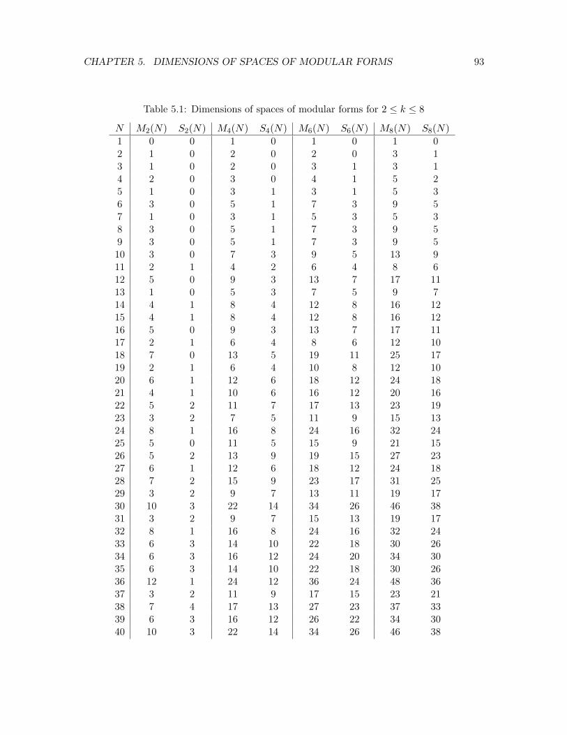
CHAPTER 5. DIMENSIONS OF SPACES OF MODULAR FORMS 93
Table 5.1: Dimensions of spaces of modular forms for 2 ≤ k ≤ 8
N M2(N) S2(N) M4(N) S4(N) M6(N) S6(N) M8(N) S8(N)
1 0 0 1 0 1 0 1 02 1 0 2 0 2 0 3 13 1 0 2 0 3 1 3 14 2 0 3 0 4 1 5 25 1 0 3 1 3 1 5 36 3 0 5 1 7 3 9 57 1 0 3 1 5 3 5 38 3 0 5 1 7 3 9 59 3 0 5 1 7 3 9 510 3 0 7 3 9 5 13 911 2 1 4 2 6 4 8 612 5 0 9 3 13 7 17 1113 1 0 5 3 7 5 9 714 4 1 8 4 12 8 16 1215 4 1 8 4 12 8 16 1216 5 0 9 3 13 7 17 1117 2 1 6 4 8 6 12 1018 7 0 13 5 19 11 25 1719 2 1 6 4 10 8 12 1020 6 1 12 6 18 12 24 1821 4 1 10 6 16 12 20 1622 5 2 11 7 17 13 23 1923 3 2 7 5 11 9 15 1324 8 1 16 8 24 16 32 2425 5 0 11 5 15 9 21 1526 5 2 13 9 19 15 27 2327 6 1 12 6 18 12 24 1828 7 2 15 9 23 17 31 2529 3 2 9 7 13 11 19 1730 10 3 22 14 34 26 46 3831 3 2 9 7 15 13 19 1732 8 1 16 8 24 16 32 2433 6 3 14 10 22 18 30 2634 6 3 16 12 24 20 34 3035 6 3 14 10 22 18 30 2636 12 1 24 12 36 24 48 3637 3 2 11 9 17 15 23 2138 7 4 17 13 27 23 37 3339 6 3 16 12 26 22 34 3040 10 3 22 14 34 26 46 38

CHAPTER 5. DIMENSIONS OF SPACES OF MODULAR FORMS 94
Table 5.2: Dimensions of spaces of modular forms for 10 ≤ k ≤ 16
N M10(N) S10(N) M12(N) S12(N) M14(N) S14(N) M16(N) S16(N)
1 1 0 2 1 1 0 2 12 3 1 4 2 4 2 5 33 4 2 5 3 5 3 6 44 6 3 7 4 8 5 9 65 5 3 7 5 7 5 9 76 11 7 13 9 15 11 17 137 7 5 9 7 9 7 11 98 11 7 13 9 15 11 17 139 11 7 13 9 15 11 17 1310 15 11 19 15 21 17 25 2111 10 8 12 10 14 12 16 1412 21 15 25 19 29 23 33 2713 11 9 15 13 15 13 19 1714 20 16 24 20 28 24 32 2815 20 16 24 20 28 24 32 2816 21 15 25 19 29 23 33 2717 14 12 18 16 20 18 24 2218 31 23 37 29 43 35 49 4119 16 14 20 18 22 20 26 2420 30 24 36 30 42 36 48 4221 26 22 32 28 36 32 42 3822 29 25 35 31 41 37 47 4323 19 17 23 21 27 25 31 2924 40 32 48 40 56 48 64 5625 25 19 31 25 35 29 41 3526 33 29 41 37 47 43 55 5127 30 24 36 30 42 36 48 4228 39 33 47 41 55 49 63 5729 23 21 29 27 33 31 39 3730 58 50 70 62 82 74 94 8631 25 23 31 29 35 33 41 3932 40 32 48 40 56 48 64 5633 38 34 46 42 54 50 62 5834 42 38 52 48 60 56 70 6635 38 34 46 42 54 50 62 5836 60 48 72 60 84 72 96 8437 29 27 37 35 41 39 49 4738 47 43 57 53 67 63 77 7339 44 40 54 50 62 58 72 6840 58 50 70 62 82 74 94 86
Chapter 6
Hecke operators
Recall the conjecture of Ramanujan that τ(mn) = τ(m)τ(n) form,n relatively prime. Whilethis specific result was shown by Mordell, it was Hecke who developed a general theory todetermine which modular forms have multiplicative Fourier coefficients (i.e., amn = amanwhenever gcd(m,n) = 1—note this imposes no condition on a0). Note that if the Fouriercoefficients an of some modular form are multiplicative, then they are determined by a0 andthe prime power Fourier coefficients apr .
The following elementary exercise shows the Eisenstein series series Ek essentially havemultiplicative Fourier coefficients.
Exercise 6.0.1. If gcd(m,n) = 1, show σk(m)σk(n) = σk(mn).
Namely, if we write
Ek(z) = 1− 2k
Bk
∑n≥1
σk−1(n)qn =∑
anqn,
the above exercise shows
aman =
(2k
Bk
)2
σk−1(m)σk−1(n) =
(2k
Bk
)2
σk−1(mn) = − 2k
Bkamn = a1amn.
Or, if we simply consider the renormalized Eisenstein series,
E∗k(z) = −Bk2k
(z)Ek(z) = −Bk2k
+∑n≥1
σk−1(n)qn, (6.0.1)
we see E∗k has multiplicative Fourier coefficients. Now we can say that by “essentially mul-tiplicative” Fourier coefficients, we mean some nonzero multiple of our modular form hasmultiplicative Fourier coefficients.
Hecke’s idea for determining if a modular form has (essentially) multiplicative Fouriercoefficients, very roughly, is the following. Consider an operator
Up
(∑anq
n)
=∑
apnqn. (6.0.2)
95

CHAPTER 6. HECKE OPERATORS 96
If this operator preserves S12(1), then
Up∆ = λp∆
for some λp ∈ C, since S12(1) = 〈∆〉. On the other hand,
Up∆ = Up(q − 24q2 + 252q3 − · · · ) = τ(p)q − 24τ(p)q2 + · · ·
so λp = τ(p) and therefore we would have τ(pn) = τ(p)τ(n) for all n.However, τ is not totally multiplicative, i.e., τ(p2) 6= τ(p)2, so Up does not preserve
∆. Instead, since Ramanujan predicted τ(p2) = τ(p)2 − p11, one would expect τ(pn) =τ(p)τ(n) − p11τ(n/p) for p|n. Thus one can guess the correct operator (for weight 12)should be
Tp
(∑anq
n)
=∑p-n
apnqn +
∑p|n
(apn + p11an/p
)qn. (6.0.3)
Then one just needs to show Tp preserves S12(1).
6.1 Hecke operators for Γ0(N)
While we could define the Hecke operators directly by their action on Fourier expansionsalong the lines of (6.0.3), it will be helpful (and more motivated) to think of them as actingon lattices.
First let’s consider the case of PSL2(Z). Recall PSL2(Z)\H parameterizes the space oflattices up to homothety (equivalence by C×). Hence a weak modular form of weight 0 issimply a meromorphic function on equivalence classes of lattices.
What about weight k? Given f ∈ Mk(1), consider the lattice Λ = 〈1, τ〉 with τ ∈ H.Put F (Λ) = f(τ). Since 〈ω1, ω2〉 = 〈ω′1, ω′2〉 if and only if(
a bc d
)(ω1
ω2
)=
(ω′1ω′2
)one easily sees that 〈1, τ〉 = 〈1, τ ′〉 (with τ ′ ∈ H also) if and only if τ ′ = τ + d for somed ∈ Z. Thus f having period 1 implies F (Λ) is well-defined on lattices of the form 〈1, τ〉.
Now consider an arbitrary lattice Λ = 〈ω1, ω2〉. We can write Λ = ω1〈1, ω2/ω1〉 = λ〈1, τ〉where λ = ω1 and τ = ω2/ω1. Thus, to see how to extend F to a function on all lattices itsuffices to determine how F should behave under multiplying a lattice Λ = 〈1, τ〉 by a scalarλ. It’s reasonable to ask that a scalar λ should just transform F by some factor, i.e.,
F (λΛ) = c(λ)F (Λ).
The only condition we have is that this should be compatible with our definition of F (〈1, τ〉) =f(τ). In other words, if λ〈1, τ ′〉 = 〈1, τ〉, we need to ensure F (λ〈1, τ ′〉) = F (〈1, τ〉).
This boils down to the case where λ = τ and τ ′ = − 1τ . Here we require
c(τ)f
(−1
τ
)= F (τ〈1, 1
τ〉) = F (〈1, τ〉) = f(τ).
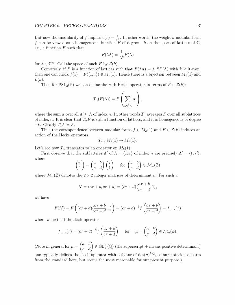
CHAPTER 6. HECKE OPERATORS 97
But now the modularity of f implies c(τ) = 1τk. In other words, the weight k modular form
f can be viewed as a homogeneous function F of degree −k on the space of lattices of C,i.e., a function F such that
F (λΛ) =1
λkF (Λ)
for λ ∈ C×. Call the space of such F by L(k).Conversely, if F is a function of lattices such that F (λΛ) = λ−kF (Λ) with k ≥ 0 even,
then one can check f(z) = F (〈1, z〉) ∈Mk(1). Hence there is a bijection betweenMk(1) andL(k).
Then for PSL2(Z) we can define the n-th Hecke operator in terms of F ∈ L(k):
Tn(F (Λ)) = F
∑Λ′n⊂Λ
Λ′
,
where the sum is over all Λ′ ⊆ Λ of index n. In other words Tn averages F over all sublatticesof index n. It is clear that TnF is still a function of lattices, and it is homogeneous of degree−k. Clearly T1F = F .
Thus the correspondence between modular forms f ∈ Mk(1) and F ∈ L(k) induces anaction of the Hecke operators
Tn : Mk(1)→Mk(1).
Let’s see how Tn translates to an operator on Mk(1).First observe that the sublattices Λ′ of Λ = 〈1, τ〉 of index n are precisely Λ′ = 〈1, τ ′〉,
where (τ ′
1
)=
(a bc d
)(τ1
)for
(a bc d
)∈Mn(Z)
whereMn(Z) denotes the 2× 2 integer matrices of determinant n. For such a
Λ′ = 〈aτ + b, cτ + d〉 = (cτ + d)〈aτ + b
cτ + d, 1〉,
we have
F (Λ′) = F
((cτ + d)〈aτ + b
cτ + d, 1〉)
= (cτ + d)−kf
(aτ + b
cτ + d
)= f |µ,k(τ)
where we extend the slash operator
f |µ,k(τ) = (cτ + d)−kf
(aτ + b
cτ + d
)for µ =
(a bc d
)∈Mn(Z).
(Note in general for µ =
(a bc d
)∈ GL+
2 (Q) (the superscript + means positive determinant)
one typically defines the slash operator with a factor of det(µ)k/2, so our notation departsfrom the standard here, but seems the most reasonable for our present purpose.)
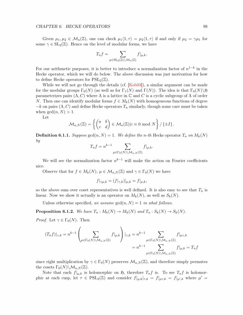
CHAPTER 6. HECKE OPERATORS 98
Given µ1, µ2 ∈ Mn(Z), one can check µ1〈1, τ〉 = µ2〈1, τ〉 if and only if µ2 = γµ1 forsome γ ∈ SL2(Z). Hence on the level of modular forms, we have
Tnf =∑
µ∈SL2(Z)\Mn(Z)
f |µ,k.
For our arithmetic purposes, it is better to introduce a normalization factor of n1−k in theHecke operator, which we will do below. The above discussion was just motivation for howto define Hecke operators for PSL2(Z).
While we will not go through the details (cf. [Kob93]), a similar argument can be madefor the modular groups Γ0(N) (as well as for Γ1(N) and Γ(N)). The idea is that Γ0(N)\Hparameterizes pairs (Λ, C) where Λ is a lattice in C and C is a cyclic subgroup of Λ of orderN . Then one can identify modular forms f ∈Mk(N) with homogeneous functions of degree−k on pairs (Λ, C) and define Hecke operators Tn similarly, though some care must be takenwhen gcd(n,N) > 1.
Let
Mn,N (Z) =
(a bc d
)∈Mn(Z)|c ≡ 0 mod N
/ ±I .
Definition 6.1.1. Suppose gcd(n,N) = 1. We define the n-th Hecke operator Tn onMk(N)by
Tnf = nk−1∑
µ∈Γ0(N)\Mn,N (Z)
f |µ,k.
We will see the normalization factor nk−1 will make the action on Fourier coefficientsnice.
Observe that for f ∈Mk(N), µ ∈Mn,N (Z) and γ ∈ Γ0(N) we have
f |γµ,k = (f |γ,k)|µ,k = f |µ,k,
so the above sum over coset representatives is well defined. It is also easy to see that Tn islinear. Now we show it actually is an operator on Mk(N), as well as Sk(N).
Unless otherwise specified, we assume gcd(n,N) = 1 in what follows.
Proposition 6.1.2. We have Tn : Mk(N)→Mk(N) and Tn : Sk(N)→ Sk(N).
Proof. Let γ ∈ Γ0(N). Then
(Tnf)|γ,k = nk−1
∑µ∈Γ0(N)\Mn,N (Z)
f |µ,k
|γ,k = nk−1∑
µ∈Γ0(N)\Mn,N (Z)
f |µγ,k
= nk−1∑
µ∈Γ0(N)\Mn,N (Z)
f |µ,k = Tnf
since right multiplication by γ ∈ Γ0(N) preservesMn,N (Z), and therefore simply permutesthe cosets Γ0(N)\Mn,N (Z).
Note that each f |µ,k is holomorphic on H, therefore Tnf is. To see Tnf is holomor-phic at each cusp, let τ ∈ PSL2(Z) and consider f |µ,k|τ,k = f |µτ,k = f |µ′,k where µ′ =

CHAPTER 6. HECKE OPERATORS 99
µτ =
(a bc d
)∈ Mn(Z) (but not necessarily Mn,N (Z)). As Im(z) → ∞, f |µ′,k(z) →
limIm(z)→∞1
(cz)kf(ac
)which has a finite limit because f is holomorphic at the cusp a
c . Thuseach f |µ′ is holomorphic at i∞, and Tnf is holomorphic at the cusps.
The same argument we used for holomorphy at the cusps shows that, if f vanishes atthe cusps, so does Tnf .
Lemma 6.1.3. A set of coset representatives for Γ0(N)\Mn,N (Z) is(a b0 d
): a, d > 0, ad = n, 0 ≤ b < d
.
Proof. Take(a bcN d
)∈ Mn,N (Z) representing some coset in Γ0(N)\Mn,N (Z). Since
gcd(n,N) = 1, we know gcd(a, cN) = 1. Then there exist x, y ∈ Z such that(x ycN −a
)∈
Γ0(N). Now observe(x ycN −a
)(a bcN d
)=
(ax+ cyN bx+ dy
0 bcN − ad
),
which means we may assume c = 0 for our coset representative.
Further, given(a b0 d
)∈Mn,N (Z), we may replace it by the coset representative
(1 x0 1
)(a b0 d
)=
(a b+ dx0 d
)where we choose x so that 0 ≤ b + dx < d, i.e., we may just assume 0 ≤ b < d. Sincen = ad > 0, a and d have the same sign, we may multiply by −I if necessary to assumea, d > 0. This shows any coset has a representative of the desired form.
Now consider(a b0 d
)and
(a′ b′
0 d′
)such that ad = a′d′ = n, 0 ≤ b < d and 0 ≤ b′ < d′.
Assume they represent the same coset, i.e.,(a′ b′
0 d′
)=
(r stN u
)(a b0 d
)=
(ra rb+ sdtNa tNb+ ud
)
for some(r stN u
)∈ Γ0(N). First we see this means t = 0, which means r = u = 1 (up to
±1). This means a′ = a d′ = d, and b′ = b + sd. However 0 ≤ b′ < d′ = d implies we need
s = 1, i.e.,(r stN u
)= I, and therefore any two distinct matrices of the prescribed form
represent distinct cosets.
Theorem 6.1.4. Let f(z) =∑anq
n ∈Mk(N) and suppose gcd(m,N) = 1. Then
(Tmf)(z) =∑
bnqn

CHAPTER 6. HECKE OPERATORS 100
wherebn =
∑d| gcd(m,n)
dk−1amn/d2 .
In particular, if m = p is prime, then
bn =
apn p - napn + pk−1an/p p|n
so(Tpf)(z) =
∑n6≡0 mod p
apnqn +
∑n≡0 mod p
(apn + pk−1an/p
)qn.
Proof. By the previous lemma, we have
(Tmf)(z) = mk−1∑
f |a b0 d
,kwhere the sum runs over a, b, d ∈ Z≥0 such that ad = m and 0 ≤ b < d. Note
f |a b0 d
,k(z) =1
dkf
(az + b
d
)=
1
dk
∞∑n=0
ane2πia
dzne2πi b
dn =
1
dk
∞∑n=0
ζbnd anqadn.
For fixed a, d we will be considering the sum
∑0≤b<d
1
dkf
(az + b
d
)=
1
dk
∞∑n=0
∑0≤b<d
ζbnd
anqadn.
Note that the inner sum∑
0≤b<d ζbnd will just be a sum over all d-th roots of unity, and
therefore vanish, unless d|n, in which case it is just d. Thus
∑0≤b<d
1
dkf
(az + b
d
)=
1
dk−1
∞∑n=0
adnqan.
Hence
(Tmf)(z) = mk−1∑ad=m
∑0≤b<d
1
dkf
(az + b
d
)= mk−1
∑ad=m
(1
dk−1
∞∑n=0
adnqan
)
=∞∑n=0
∑a|m
(ak−1amn/aq
an)
=∞∑n=0
∑d|m
dk−1amn/d2qn.
Corollary 6.1.5. The Ramanujan tau function satisfies τ(mn) = τ(m)τ(n) whenevergcd(m,n) = 1 and τ(pr) = τ(p)τ(pr−1)− p11τ(pr−2).
CHAPTER 6. HECKE OPERATORS 101
Proof. Consider
(Tp∆)(z) =∑p-n
τ(pn)qn +∑p|n
(τ(pn) + p11τ(n/p)
)qn.
On the other hand, Tp acts on S12(1) = C∆ so
(Tp∆)(z) = λ∆(z)
for some λ ∈ C×. The 1st Fourier coefficients of ∆ and Tp∆ are just 1 and τ(p), so λ = τ(p).Comparing the n-th Fourier coefficients, we see
τ(pn) = λτ(n) = τ(p)τ(n) p - nτ(pn) + p11τ(n/p) = λτ(n) = τ(p)τ(n) p|n.
The former equation proves the multiplicativity when m = p and the latter equation provesthe recursion relation for τ(pr).
To obtain the general multiplicativity law τ(mn) = τ(m,n) for gcd(m,n) = 1, we simplyuse the same argument as above with Tm instead of Tp.
The above argument applies in a more general setting.
Exercise 6.1.6. Suppose f(z) =∑anq
n ∈ Sk(N) (resp. Mk(N)) and dimSk(N) = 1 (resp.dimMk(N) = 1). Show
(i) If gcd(m,N) = gcd(n,N) = gcd(m,n) = 1, then a1amn = aman. In particular,if f(z) 6= 0 we must have a1 6= 0, and if we normalize f such that a1 = 1, the Fouriercoefficients are multiplicative.
(ii) If a1 = 1 and p - N , then apn = apapn−1 − pk−1apn−2 for n ≥ 2.
What this means is we can use Hecke operators to compute values of Fourier coefficientsfrom just knowing what the Tp’s are.
Exercise 6.1.7. Using the fact that dimS16(1) = 1, use the previous exercise to help com-pute the first 10 Fourier coefficients of E4∆.
Now you might ask, for what modular forms f are the Fourier coefficients multiplicativein the sense a1amn = aman for gcd(m,n) = 1? By Exercise 6.0.1, we know this is true forthe Eisenstein series Ek, and now we have seen it is true for ∆, and by Exercise 6.1.6, anyEk∆ where k = 4, 6, 8, 10, 14.
In general, if you have two power series (or Fourier expansions) f and g with multiplica-tive coefficients, the formal product fg will not have multiplicative Fourier coefficients, sothere is no reason to expect all modular forms—or even products of modular forms withmultiplicative Fourier coefficients—to have multiplicative coefficients. For instance, startingin weight 24 for the full modular group, we have a space of cusp forms of dimension greaterthan 1, namely S24(1) = 〈∆2, E12∆〉. Since
∆(z) = q − 24q2 + 252q3 − 1472q4 + 4830q4 − 6048q6 + · · ·

CHAPTER 6. HECKE OPERATORS 102
we compute∆2(z) = q2 − 48q3 + 1080q4 − 2944q5 + 143820q6 + · · · .
Right away, we see two things: 1) the Fourier coefficients of q2 and q3 do not multiply togive the Fourier coefficient of q6, and 2) a1 = 0 so the multiplicative property a1an = amanfor gcd(m,n) = 1 would mean an = 0 whenever n is divisible by two different primes, whichis obviously not the case. (In fact something stronger is true, see Corollary 6.1.11 below.)
One can also check that
E12 = 1 +65520
691
(q + 2049q2 + 177148q3 + 4196353q4 + 48828126q5 + · · ·
)so
E12∆ = q +65520
691
(2039
2730q2 +
527191
260q3 +
525013709
4095q4 + · · · − 666536766
65q6 + · · ·
)While the first Fourier coefficient is 1 here, again one sees the products of the q2 and q3
coefficients does not give the q6 coefficient (it’s not even the right sign!). So one cannothope that the Fourier coefficients of Ek∆ are multiplicative in general.
You might now ask, are there any elements of S24(1) with multiplicative Fourier coeffi-cients or does this property of having multiplicative Fourier coefficients only occur in smallweight? We will see there always are cusp forms with multiplicative Fourier coefficients.First, let’s make an observation in the weight 12 case: while 691
65520E12 and ∆ have multi-plicative Fourier coefficients, one can’t expect this for any modular form in M12(1). Namelyif f and g have multiplicative Fourier coefficients, f + g will generally not. So while mostforms in M12(1) do not have multiplicative Fourier coefficients, M12(1) is generated by two“nice” forms, 691
65520E12 and ∆, which do.Using the theory of Hecke operators, we will show that there exists such a “nice” basis
for Mk(N) and Sk(N). The basic idea is to show that the Hecke operators Tm and Tncommute for gcd(m,n) = 1 (and m,n prime to N). Then one defines an inner product〈·, ·〉, called the Petersson inner product, on Mk(N) and shows each Tn is Hermitian withrespect to 〈·, ·〉, i.e., 〈Tnf, g〉 = 〈f, Tng〉. Then a well known theorem in linear algebra saysthat a commuting family of operators which are Hermitian with respect to 〈·, ·〉 can besimultaneously diagonalized by some orthonormal basis with respect f1, . . . , fr to 〈·, ·〉 Inother words, each fi is an eigenform for Tn, i.e., Tnfi = λfi for some λ ∈ C.
Definition 6.1.8. Let f ∈ Mk(N) be nonzero. We say f is a (Hecke) eigenform if,for each n relatively prime to N , there exists a (Hecke) eigenvalue λn ∈ C such thatTnf = λnf .
We say f is a normalized eigenform if the first nonzero Fourier coefficient is 1.
The arguments from Corollary 6.1.5 and Exercise 6.1.6 apply to show any Hecke eigen-form has multiplicative Fourier coefficients. Precisely, work out
*Exercise 6.1.9. Let f =∑anq
n ∈ Mk(N) be a Hecke eigenform. Suppose gcd(m,n) =gcd(m,N) = gcd(n,N) = 1. Then a1amn = aman.

CHAPTER 6. HECKE OPERATORS 103
In other words, the basis f1, . . . , fr which diagonalizes the Tn’s asserted above is a basisof Hecke eigenforms, and therefore a basis of Mk(N) with multiplicative Fourier coefficientsin the sense of the previous exercise.
We remark that there is a technicality here we have ignored, namely that the Peterssoninner product 〈f, g〉 is only well defined when at least f or g is a cusp form. So the aboveargument will only technically show that Sk(N) has a basis of eigenforms but, at least whenN = 1, we will see how this implies one can extend the basis of eigenforms of Sk(N) to abasis of eigenforms for Mk(N).
We remark that for a eigencusp form (a Hecke eigenform which is a cusp form) the firstnonzero Fourier coefficient should be a1 in order for the Hecke operators to not force everyFourier coefficient to be zero.
Lemma 6.1.10. Let f =∑anq
n ∈Mk(1) be a Hecke eigenform and k > 0. Then a1 6= 0.
Proof. Write Tmf = λmf =∑bnq
n. Then b1 = am. Consequently
am = λma1.
In other words, if a1 = 0, then am = 0 for all n ≥ 0. Consequently f(z) = a0 ∈M0(1).
Corollary 6.1.11. Let f ∈Mk(1). Then ∆2f is not a Hecke eigenform.
In particular, this shows ∆2 is not an eigenform.
Now let’s get to the first step in showing the existence of Hecke eigenforms, which isshowing the Hecke operators are commutative.
Lemma 6.1.12. Suppose gcd(m,N) = gcd(n,N) = 1 and gcd(m,n) = 1. Then the Heckeoperators on Mk(N) satisfy TmTn = Tmn.
Proof. Take f(z) =∑arq
r ∈ Mk(N). Write Tnf(z) =∑brq
r and Tm(Tnf)(z) =∑crq
r.Then
br =∑
d| gcd(n,r)
dk−1anr/d2
socr =
∑e| gcd(m,r)
ek−1bmr/e2 =∑
e| gcd(m,r)
ek−1∑
d| gcd(n,mr/e2)
dk−1amnr/d2e2 .
Since gcd(m,n) = 1, d runs over the divisors of gcd(n, r/e), and therefore d′ = de runs overthe divisors of mn and
cr =∑
d′| gcd(mn,r)
(d′)k−1amnr/(d′)2
so TmTn = Tmn.
Lemma 6.1.13. Suppose p - N . The Hecke operators on Mk(N) satisfy
TprTps =∑
d| gcd(pr,ps)
dk−1Tpr+s/d2 . (6.1.1)

CHAPTER 6. HECKE OPERATORS 104
Proof. The proof here is modeled on the one in [Apo90, Theorem 6.13], but there appear tome to be errors in the r = 1 case of loc. cit. I believe I have corrected them.
We may as well assume r ≤ s.First let’s show the r = 1 case, which just says
TpTps = Tps+1 + pk−1Tps−1 .
For f ∈Mk(n),
Tpsf(z) = ps(k−1)∑
0≤i≤s
∑0≤b<pi
f |ps−i b0 pi
,k= ps(k−1)
∑0≤i≤s
p−ik∑
0≤b<pif
(ps−iz + b
pi
). (6.1.2)
In particular
Tpg(z) = p(k−1)g(pz) + p−1∑
0≤b′<pg
(z + b′
p
)so
TpTpsf(z) = p(s+1)(k−1)∑
0≤i≤sp−ik
∑0≤b<pi
f
(ps+1−iz + b
pi
)(6.1.3)
+ p−1ps(k−1)∑
0≤b′<p
∑0≤i≤s
p−ik∑
0≤b<pif
(ps−i(z + b′) + pb
pi+1
). (6.1.4)
Note the i = s term from (6.1.4) is
p−1−s∑
0≤b′<p
∑0≤b<ps
f
(z + b′ + pb
ps+1
)= p−1−s
∑0≤b<ps+1
f
(z + b
ps+1
).
Thus adding the i = s term from (6.1.4) to (6.1.3) gives (6.1.2) with s replaced by s + 1,i.e., they sum to Tps+1f(z).
Now the remaining terms, i.e., the i < s terms from (6.1.4), sum to
p−1ps(k−1)∑
0≤b′<p
∑0≤i≤s−1
p−ik∑
0≤b<pif
(ps−1−iz + b+ ps−1−ib′
pi
)
If i ≤ s−12 , then ps−1−ib′
pi∈ Z, so by periodicity of f there is no dependence on b′ and the
contribution for such a fixed i is
ps(k−1)p−ik∑
0≤b<pif
(ps−1−iz + b
pi
). (6.1.5)
In fact, for any i, b + ps−1−ib′ mod pi runs over the set of residue classes mod pi exactly ptimes, so the contribution for any i is given again by (6.1.5). This proves the r = 1 case.

CHAPTER 6. HECKE OPERATORS 105
Now we suppose (6.1.1) is true up to some fixed r. By the r = 1 case we have
Tpr+1Tps = (TpTpr)Tps − pk−1Tpr−1Tps .
By the inductive assumption that (6.1.1) is true for r, we also have
Tp (TprTps) =∑
0≤i≤rpi(k−1)TpTpr+s−2i .
Comparing these, and making another use of the r = 1 case, gives
Tpr+1Tps =∑
0≤i≤rpi(k−1)TpTpr+s−2i − pk−1Tpr−1Tps
=∑
0≤i≤r
(pi(k−1)Tpr+s+1−2i + p(i+1)(k−1)Tpr+s−1−2i
)− pk−1Tpr−1Tps .
Expanding out the last term using the r − 1 case of (6.1.1) gives
Tpr+1Tps =∑
0≤i≤r+1
pi(k−1)Tpr+s+1−2i .
The previous two lemmas combine to give the following.
Corollary 6.1.14. The Hecke operators Tngcd(n,N)=1 on Mk(N) commute.
The former lemma also shows knowing what the prime power Hecke operators do tellsyou what all Hecke operators do, and the latter lemma shows that the prime power Heckeoperators are determined by the prime Hecke operators. In particular, we see
Corollary 6.1.15. If f ∈ Mk(N) is an eigenform for each Tp with p - N prime, i.e.,Tpf = λpf for some λp ∈ C, then f is a Hecke eigenform.
Proof. The r = 1 case of (6.1.1) says, for j = s− 1 ≥ 2,
Tpj = TpTpj−1 − pk−1Tpj−2 .
If Tpif = λpif for some λpi whenever i < j, then we see
Tpjf = Tp(λpj−1f)− pk−1λpj−2f = λpjf
whereλpj =
(λpλpj−1 − pk−1λpj−2
). (6.1.6)
Hence by induction, we see if Tpf = λpf then Tpjf = λpjf for some λpj—precisely, with λjpsatisfying the recursion in (6.1.6).
Now let n be relatively prime to N , and write n = pe11 . . . perr . By Lemma 6.1.12, we have
Tnf =
(r∏i=1
Tpeii
)f =
r∏i=1
λpeiif.
CHAPTER 6. HECKE OPERATORS 106
6.2 Petersson inner product
We know thatMk(Γ) is a finite dimensional complex vector space, and therefore can be madeinto a Hilbert space, i.e., an inner product space. The standard way to make a functionspace into a Hilbert space is with the L2 inner product. Namely, if f, g ∈ L2(X) for somespace X, then the inner product is given by
〈f, g〉 =
∫Xf(x)g(x) dx.
While modular forms are not L2 on H, they are essentially L2 on relevant Riemannsurface X = Γ\H. We say essentially here, because they are of course not actually functionson Γ\H due to the automorphy transformation factor except in the uninteresting (constant)case of k = 0.
Let’s see what happens when we naively try to make f ∈ Mk(Γ) into a function onX = Γ\H. For simplicity, consider Γ = PSL2(Z) = 〈S, T 〉. We already have f(Tz) =f(z + 1) = f(z) so f descends to a function on the infinite cylinder 〈T 〉\H. We would liketo modify f to a function F = Ff which still satisfies F (z + 1) = F (z) but also satisfiesF (Sz) = F (−1/z) = F (z).
Since the invariance under T is a transformation rule in x = Re(z) which we don’t wantto mess up, we might just try to impose invariance under S by modifying y = Im(z). Sincef(S · iy) = f(−1/iy) = f(i/y) = (iy)kf(iy), it makes sense to consider the function (whichwill be called a Maass form)
F (z) := yk/2f(z) = Im(z)k/2f(z). (6.2.1)
Then we still have F (z + 1) = F (z) for all z and now
F (−1/iy) = F (i/y) = y−k/2f(i/y) = ±ikyk/2f(iy) = (−1)k/2F (iy),
so at least F (−1/iy) = F (iy) when k ≡ 0 mod 4. (One could let F (z) = (iy)k/2f(z) sothat we actually have F (−1/iy) = F (iy), but one typically considers F as defined in (6.2.1),since the sign (−1)k/2 will not matter in the end.) It doesn’t quite satisfy F (−1/z) = F (z)for all z but it will be close, and we can say how close.
In general, for any f ∈ Mk(Γ), we can associate to f the Maass form F defined by(6.2.1). Noting that
|j(γ, z)|2 =Im(z)
Im(γz), γ ∈ SL2(R) (6.2.2)
(cf. (3.2.1)), we see
F (γz) = Im(γz)k/2f(γz) = Im(γz)k/2j(γ, z)kf(z) = j0(γ, z)kIm(z)k/2f(z) = j0(γ, z)kF (z)
for γ ∈ Γ, where
j0(γ, z) =j(γ, z)
|j(γ, z)|.

CHAPTER 6. HECKE OPERATORS 107
In other words, the Maass form F (not holomorphic) is not quite invariant under Γ, but it isup to a factor j0(γ, z) of absolute value 1. This is good enough for our purposes.1 Namely, ifalso g ∈Mk(Γ) and G(z) = Im(z)k/2g(z) is the associated Maass form, it means the product
F (γz)G(γz) = j0(γ, z)kj0(γ, z)kF (z)G(z) = F (z)G(z)
is invariant under Γ.Consequently, we can define the inner product
〈f, g〉 =
∫Γ\H
F (z)G(z) dω,
where dω is an area measure on the Riemann surface X = Γ\H. Now in practice, you wantto express this as an integral on a fundamental domain for Γ inside H, so we need to knowwhat the hyperbolic measure should be.
Lemma 6.2.1. The measure dx dyy2
= dz dzIm(z)2
is an invariant measure on the hyperbolic planeH, i.e., for γ ∈ PSL2(R) we have∫
Hf(γz)
dx dy
y2=
∫Hf(z)
dx dy
y2,
for any integrable (w.r.t. to this measure) function f on H.
Proof. Write γ =
(a bc d
), and let
w = γz =(ad+ bc)x+ bd+ acy2 + iy
c2x2 + c2y2 + d2= u+ iv.
Notedw
dz=
1
|cz + d|2=∂u
∂x+ i
∂v
∂x=∂v
∂y− i∂u
∂y.
Then the Jacobian determiant∣∣∣∣∂x∂u ∂y∂u
∂x∂v
∂y∂v
∣∣∣∣ =
∣∣∣∣∣∂u∂x ∂u∂y
∂v∂x
∂v∂y
∣∣∣∣∣−1
=
∣∣∣∣|cz + d|−2 00 |cz + d|−2
∣∣∣∣−1
= |j(γ, z)|4.
Since |j(γ, z)|2 = Im(z)Im(γz) = y
v , we have∫Hf(γz)
dx dy
y2=
∫Hf(w)|j(γ, z)|4 du dv
y2=
∫Hf(w)
du dv
v2.
1We remark that one can make f invariant under Γ at the expense of working on a larger space thanH. Namely, one has the surjective map PSL2(R) → H given by γ 7→ γ · i. Since SO(2) stabilizes i, onecan view PSL2(R)/SO(2) ' H. Thus one can lift f to a function on PSL2(R) by f(γ) = f(γ · i) and definethe automorphic form φf (γ) = j(γ, i)k/2f(γ). This makes φf invariant under Γ so it is a function onΓ\PSL2(R). Hence, viewed as functions on PSL2(R), the passage from modular forms to automorphic formstrades right SO(2) invariance for left Γ invariance.

CHAPTER 6. HECKE OPERATORS 108
Definition 6.2.2. Let f, g ∈Mk(Γ). The Petersson inner product of f with g is definedto be
〈f, g〉 :=1
[PSL2(Z) : Γ]
∫Γ\H
ykf(z)g(z)dx dy
y2(6.2.3)
whenever the integral converges.
The above discussion shows that the integrand is invariant under Γ, so the definingintegral makes sense, provided it converges. Consequently, we can also write this integral as
〈f, g〉 :=1
[PSL2(Z) : Γ]
∫Fykf(z)g(z)
dx dy
y2(6.2.4)
where F is any fundamental domain for Γ.The normalization factor [PSL2(Z) : Γ]−1 roughly cancels out the volume of Γ\H, defined
to bevol(Γ\H) =
∫Γ\H
dx dy
y2.
Lemma 6.2.3. Let Γ be a congruence subgroup in PSL2(Z). Then vol(Γ\H) is finite.
Proof. Let F ′ be a fundamental domain for Γ. By Lemma 3.4.9,
F ′ =[PSL2(Z):Γ]⋃
i=1
αiF ,
where F is the standard fundamental domain for PSL2(Z) and αi ∈ PSL2(Z). Since thearea measure is invariant under the action of PSL2(R),
vol(F ′) =∑
vol(αiF) = [PSL2(Z) : Γ]vol(F),
so it suffices to show F has finite volume. Note
vol(F) =
∫ 1/2
−1/2
∫ ∞√
1−x2
dx dy
y2≤∫ 1/2
−1/2
∫ ∞1/2
dx dy
y2= 2
∫ 1/2
−1/2dx = 2.
The proof is of course valid not just for congruence subgroups, but any finite indexsubgroup of PSL2(Z), and consequently any subgroup of PSL2(R) commensurable withPSL2(Z).
Exercise 6.2.4. Compute vol(X0(1)) = vol(PSL2(Z)\H).
Note the above lemma implies the Petersson inner product converges for (the admittedlynot very interesting case of) f, g ∈ M0(Γ) = C. However for general weight k we do notalways have convergence. For instance, in the standard fundamental domain of PSL2(Z),the yk can grow too fast for the Petersson inner product to converge unless f(z)g(z)→ 0 asy → ∞. Similarly, if we tend to a cusp in Q, f(z)g(z) may grow too fast (cf. Section 4.3)for the inner product to converge. This suggests that when k > 0 we need f or g to be acusp form for 〈f, g〉 to converge.

CHAPTER 6. HECKE OPERATORS 109
Proposition 6.2.5. Let f, g ∈ Mk(Γ). The Petersson inner product 〈f, g〉 converges ifeither f ∈ Sk(Γ) or g ∈ Sk(Γ).
Proof. We assume f ∈ Sk(Γ). The case g ∈ Sk(Γ) is similar.Let F be a fundamental domain for Γ\H and F be its closure in H. Write F = K∪
⋃Ui,
where this is a finite union of subsets with K compact in H and each Ui ⊂ H containingexactly one cusp, say zi. Since yk−2f(z)g(z) is bounded on K it suffices to show this isbounded on each Ui.
As in the proof of Lemma 4.5.8, we know f(z)→ 0 exponentially fast as z → zi, whereasyk−2g(z) has at most a finite order pole at zi. Thus yk−2f(z)g(z) is bounded on each Ui,and because vol(F) = vol(F) <∞, the Petersson inner product converges.
What this means is that the Petersson inner product defines an inner product (it is clearlysesquilinear, i.e., linear in the first vector and anti, or conjugate, linear in the second) onthe space of cusp forms Sk(N). This inner product almost extends to an inner product onMk(N), but 〈f, g〉 need not converge when both f and g are not cusp forms.
While we have failed to make Mk(N) a Hilbert space, we have at least made Sk(N) one.Most importantly, the inner product behaves symmetrically with respect to the action ofthe Hecke operators.
Lemma 6.2.6. There exists a complete set of representatives µi for Γ0(N)\Mn,N (Z) suchthat
nµ−1
i
is also a complete set of representatives for Γ0(N)\Mn,N (Z).
Proof. First we note that both Γ0(N)\Mn,N (Z) andMn,N (Z)/Γ0(N) (which equals σ1(n) =∑d|n d by Lemma 6.1.3). This follows because the map µ 7→ nµ−1, which mapsMn,N (Z) to
itself, induces a bijection of the right cosets Γ0(N)\Mn,N (Z) with the left cosetsMn,N (Z)/Γ0(N).Then we can write
Mn,N (Z) =
r⊔i=1
Γ0(N)αi =
r⊔i=1
βiΓ0(N),
for some collections, αi and βj inMn,N (Z). It is easy to see there must be a permutationπ : 1, . . . , r → 1, . . . , r such that Γ0(N)αi ∩ βπ(i)Γ0(N) 6= ∅ for all i (otherwise there isa proper subset of indices i such that Γ0(N)αi =Mn,N (Z)).
Take µi ∈ Γ0(N)αi ∩βπ(i)Γ0(N) for i = 1, . . . , r. Then µi forms a complete set of rep-resentatives both for Γ0(N)\Mn,N (Z) and forMn,N (Z)/Γ0(N). The latter fact composedwith the map µ 7→ nµ−1 shows that
nµ−1
i
is also a complete set of representatives for
Γ0(N)\Mn,N (Z).
Note: even for n = p, the representatives given in Lemma 6.1.3, do not satisfy theconditions given in the above lemma. At least some places in the literature are sloppyabout this, and as a consequence have a gap or error in the proof of the following theorembelow (this includes an earlier version of these notes, as I originally copied this mistake fromelsewhere, and I thank Roberto Miatello for pointing this out to me—the approach of usingthe above lemma can be found in [Miy06]).

CHAPTER 6. HECKE OPERATORS 110
Theorem 6.2.7. The Hecke operators Tn on Sk(N) are hermitian with respect to thePetersson inner product, i.e.,
〈Tnf, g〉 = 〈f, Tng〉
for f, g ∈ Sk(N).
Proof. Fix a fundamental domain F for Γ0(N). For simplicity of notation, we extend 〈f, g〉by (6.2.4) to any functions on H for which the integral converges.
First we claim that for any τ =
(a bc d
)∈ PSL2(R), we have
〈f |τ,k , g〉 = det(τ)−k〈f, g|τ−1,k〉,
where we extend |τ,k to τ ∈ GL2(R)+ = α ∈ GL2(R) : det(α) > 0 by (4.3.1). (The con-dition of positive determinant ensures τ maps H to H. We remark that if we had followedstandard notation and included a factor of det(τ)k/2 in our definition of the slash operator,the determinant factor would not appear in the above identity.)
This follows since
ykf |τ,k(z) g(z) =Im(z)k
(cz + d)kf(τz)g(z) = det(τ)−kIm(w)k(cz + d)
kf(w)g(τ−1w).
where we put w = τz and used the identity
|j(τ, z)|2 = det(τ)Im(z)
Im(τz), τ ∈ GL2(R)+,
which is a simple generalization of (6.2.2). Then observing (cz+d)k = j(τ, z)k = j(τ−1, w)−k
shows this equalsdet(τ)−kIm(w)kf(w)g|τ−1,k(w),
which implies our claim.Recall
Tnf = nk−1∑
µ∈Γ0(N)\Mn,N (Z)
f |µ,k = nk−1r∑i=1
f |µi,k,
where µ1, . . . , µr is a set of representatives for Γ0(N)\Mn,N (Z), which we take to be as inLemma 6.2.6. Now
〈Tnf, g〉 = nk−1∑〈f |µi,k, g〉 = n−1
∑〈f, g|µ−1
i ,k〉
Since g|nτ,k = n−kg|τ,k, this implies
〈Tnf, g〉 = nk−1∑〈f, g|nµ−1
i ,k〉 = 〈f, Tng〉,
by our choice of µi.
Corollary 6.2.8. The space Sk(N) has a basis consisting of Hecke eigenforms.

CHAPTER 6. HECKE OPERATORS 111
Proof. Since Tn is a family of commuting operators which are hermitian with respect to〈·, ·〉, a well known theorem in linear algebra tells us that an orthonormal basis with respectto 〈·, ·〉 is a basis of eigenvectors for all Tn.
By Exercise 6.1.9, we know the normalized (a1 = 1) Hecke eigenforms in Sk(N) haveFourier coefficients an which are multiplicative for n relatively prime to the level N . Hencethe cusp forms are generated by forms whose Fourier coefficients are some kind of arithmeticsequences.
There are some more questions we can ask at this point to push our theory further.
• Does the whole space of modular forms Mk(N) actually have a basis of Hecke eigen-forms?
• Can we define the Hecke operators Tn on Mk(N) when gcd(n,N) > 1?
• Can we actually find a basis for Sk(N) (or Mk(N)) whose Fourier coefficients an aremultiplicative for all n?
Here we will just briefly discuss these questions.First, observe that Theorem 6.2.7 is actually valid for f, g ∈ Mk(N) when 〈Tnf, g〉
converges. One can use this to deduce that Mk(N) does have a basis of eigenforms, and infact we already know it at least one case.
Example 6.2.9. The space Mk(1) has a basis of Hecke eigenforms. To see this, recallMk(1) = CEk ⊕ Sk(1). By Exercise 6.0.1, we know Ek is an eigenform, hence the basis ofeigenforms for Sk(1) can be extended to a basis of eigenforms for Mk(1).
In fact, the Eisenstein series (for Mk(N), or more generally for Mk(Γ)) are orthogonalto the space of cusp forms in the sense that 〈E, f〉 = 0 whenever E is an Eisenstein seriesand f is a cusp form. Often one uses this relation to define Eisenstein series: the space ofEisenstein series for Mk(Γ) will be the elements E ∈ Mk(Γ) such that 〈E, f〉 = 0 for allf ∈ Sk(Γ).
Next, one can define Hecke operators Tn on Mk(N) when gcd(n,N) > 1, however adefinition in terms ofMn,N (Z) is somewhat trickier as the analogue Lemma 6.1.3 is not asnice. For simplicity, let’s just talk about Tp where p|N , since all the Tn’s can be constructedout of just the Tp’s. One can define
Tpf =∑
0≤j<pf |1 j
0 p
,k,
and if f(z) =∑anq
n, one obtains
Tpf(z) =∑
apnqn.
The definition of Hecke operators can be made more uniform (including for arbitrary con-gruence subgroups Γ) by working in terms of double cosets (see, e.g., [DS05] or [Kob93]).
While the Hecke operators Tp for p|N can be defined without much trouble, one does notin general have a basis of eigenforms for Sk(N) for all Tn. Roughly the issue is the following.

CHAPTER 6. HECKE OPERATORS 112
Say N = pq with p, q distinct primes and f ∈ Sk(q) is a Hecke eigenform. In particular, f isan eigenform for Tp (on Sk(q)) Then automatically f ∈ Sk(N). However Tp on Sk(N) actsdifferently, so f is no longer an eigenform for Tp.
More generally, if d|N and f(z) ∈ Sk(N/d), then f(z), f(dz) ∈ Sk(N) and we thesubspace generated by all such elements the space Sold
k (N) of oldforms. Define the spaceof newforms Snew
k (N) to be its orthogonal complement in Sk(N) (w.r.t. the Petersson innerproduct). Then it is true that Snew
k (N) has a basis of eigenforms for all Tp, as opposedto just for p - N . However, it can happen that oldforms are also eigenform for all Tp,or that oldforms have multiplicative Fourier coefficients but are not eigenforms for all Tp.(Conversely, if f is an eigenform for all Tp, the Fourier coefficients may not be multiplicative,but they essentially are—they are if a1 = 1.)
The notion of newforms versus oldforms leads to another interesting question:
• Given some form f ∈ Sk(N), how can we determine if it comes from a form of smallerlevel or if it is a newform?
We will study all of these issues in Chapter 8.Finally we remark that the theory of Hecke operators for an arbitrary congruence sub-
group Γ is similar. See [Ste07] for how to computationally find a basis of Hecke eigenformsfor a given space Mk(Γ).

Chapter 7
L-functions
One of the main themes in modern number theory, is to associate to various objects (num-ber fields, Dirichlet characters, Galois representations, elliptic curves, modular forms) ananalytic gadget called an L-function. The idea comes from the theory of the Riemann zetafunction, so before we introduce L-functions for modular forms, we recall some basic factsabout the zeta function and Dirichlet L-functions.
NOTE: This chapter is readable, but not as complete as I would like. Specifically, I didn’thave enough time in my mind to say why you should care about L-functions of modularforms, e.g., the relation with elliptic curves and Fermat’s last theorem. I hope to somedayflesh out this chapter more.
7.1 Degree 1 L-functions
Let’s begin by reviewing the zeta function. Then we will review some facts about DirichletL-functions. Both of these are considered “degree 1” L-functions, which will be explainedlater.
7.1.1 The Riemann zeta function
First recall the Riemann zeta function is defined by
ζ(s) =∑ 1
ns(7.1.1)
for s ∈ C with Re(s) > 1. Then ζ(s) can be (uniquely) meromorphically continued to afunction of the whole complex plane with only a simple pole at s = 1. Euler (who consideredζ(s) for s real) observed
ζ(s) =∑ 1
ns=∏p
1
1− p−s. (7.1.2)
Since each factor on the right converges at s = 1, the fact that ζ(s) has a pole at s = 1implies there are infinitely many prime numbers. This is the first hint that the analyticbehaviour of ζ(s) can encodes deep arithmetic information.
113

CHAPTER 7. L-FUNCTIONS 114
One important feature of ζ(s) is its functional equation relating the values at s to thevalues at 1− s. Namely, recall the gamma function is defined by
Γ(s) =
∫ ∞0
ts−1e−sdt (7.1.3)
for Re(s) > 0. Then Γ(s) has meromorphic continuation to C with simple poles at s =0,−1,−2, . . .. Further Γ satisfies the functional equation
Γ(s+ 1) = sΓ(s)
and one easily computes from the definition that Γ(1) = 1. Hence, by induction, thefunctional equation implies Γ(n+ 1) = n! for n ∈ N.
Then the functional equation for ζ(s) can be written
ζ(s) = 2sπs−1 sin(πs
2
)Γ(1− s)ζ(1− s).
One can rewrite this functional equation more simply in terms of the completed zetafunction
Z(s) =s(s− 1)
2πs/2Γ(s
2
)ζ(s)
asZ(s) = Z(1− s).
Either way, the functional equation means one can obtain the values for ζ(s) from the valuesof ζ(1 − s). In particular, if Re(s) < 0, then Re(1 − s) > 1 so one can also use (7.1.1) toevaluate ζ(s) on the left half-plane Re(s) < 0. The in-between region, 0 ≤ Re(s) ≤ 1 iscalled the critical strip and line of symmetry Re(s) = 1
2 is called the critical line.As is now famous, the zeros of the Riemann zeta function are intimately connected with
prime numbers. Specifically, letψ(x) =
∑pk≤x
log p
be the Chebyshev function, which counts the number of prime powers up to x. Then onecan show the astounding explicit formula
ψ(x) = x−∑ρ
xρ
ρ− log 2π, (7.1.4)
where ρ runs over the zeroes of ζ(s) (including the “trivial zeroes” to the left of the thecritical strip). Consequently, if we knew where all the zeroes of ζ(s) lay, we would knowexactly where all the prime powers are. Regardless, one can already use (7.1.4) to prove theprime number theorem
π(x) := # p : p ≤ x ∼ ψ(x)
log x∼ x
log x.
The very deep Riemann hypothesis asserts that all nontrivial zeroes (all zeroes inside thecritical strip) actually lie on the critical line, and this would give an optimal bound on theerror term in the prime number theorem.

CHAPTER 7. L-FUNCTIONS 115
In another direction, special values of ζ(s) tell us interesting arithmetic information. Forinstance, Euler showed that for n ∈ N,
ζ(2n) = (−1)n+1B2n · (2π)2n
2(2n)!. (7.1.5)
One can interpret 1/ζ(2n) as the probability that 2n integers chosen at random are relativelyprime (this is a simple consequence of (7.1.2)). Based on this expression, one might ask,when n is odd, if ζ(n) = cπn for some c ∈ Q? While this is not known (even for ζ(3)), it isexpected the answer is no.
One heuristic reason why values at the even and odd integers should be different comesby looking the functional equation. Namely, the expression (7.1.5) simplifies to
ζ(1− 2n) = −B2n
2n.
Thus it appears the arithmetic of the special values of ζ(2n) is made more clear by lookingat ζ(1 − 2n). On the other hand by the function equation and that Γ(s) has poles atnegative integers, in order for ζ(s) to be holomorphic we need ζ(−2n) = 0. (These are thetrivial zeroes—note the functional equation does not produce zeroes at negative odd integersbecause then the vanishing of sin
(πs2
)cancels the pole from Γ(1 − s).) Since ζ(2n + 1)
corresponds to ζ(−2n) = 0, there is no indication that ζ(s) at positive odd integers shouldfollow the same sort of arithmetic behaviour as at positive even integers. (In light of theprobabilistic interpretation of 1/ζ(n), this is perhaps analogous to the difference betweenrk(n), i.e., ϑk(z), for k odd and even.)
7.1.2 Dirichlet L-functions
Definition 7.1.1. We say χ : Z→ C is a Dirichlet character mod N if(i) χ(n) = χ(n+N) for all n ∈ Z;(ii) χ(n) = 0 ⇐⇒ gcd(n,N) > 1;(iii) χ(1) = 1; and(iv) χ(mn) = χ(m)χ(n) for all m,n ∈ Z.
The standard way to construct a Dirichlet character is to take a character χ of (Z/NZ)×,extend it to Z/NZ by setting it to 0 on all the noninvertible residue classes, then lifting itto a function of Z. It is easy to see this satisfies the above definition, and conversely anyDirichlet character arises in such a way.
Then one defines the Dirichlet L-function for a Dirichlet character χ to be
L(s, χ) =∞∑n=1
χ(n)
ns, (7.1.6)
for Re(s) > 1. (Condition (i) in the definition implies χ is bounded, so the series convergesabsolutely for Re(s) > 1.) Since χ is multiplicative, again one an Euler product expansion
L(s, χ) =∞∑n=1
χ(n)
ns=∏p
1
1− χ(p)p−s. (7.1.7)
CHAPTER 7. L-FUNCTIONS 116
As with ζ(s), one can show L(s, χ) has meromorphic continuation to C, but this time it willin fact be entire whenver χ is a nontrivial character (i.e., does not come from the trivialcharacter of (Z/NZ)×).
Because the Dirichlet characters mod N allow one to distinguish among the differentresidue classes mod N , these Dirichlet L-functions provide a way to study primes lying inarithmetic progressions. Specifically, Dirichlet showed that L(1, χ) 6= 0 for each nontrivialχ, and used this to prove that for any b relatively prime to N , there are infinitely manyprimes of the form aN + b, a, b ∈ N.
Again in analogy with the Riemann zeta function, Dirichlet L-functions have functionalequations. If χ is a “primitive” Dirichlet character mod N , the completed Dirichlet L-function is
Λ(s, χ) =
(N
π
) s+ε2
Γ
(s+ ε
2
)L(s, χ) (7.1.8)
where ε ∈ 0, 1 is the order of χ(−1), i.e., ε = 0 if χ(−1) = 1 and ε = 1 if χ(−1) = −1.Then the functional equation reads
Λ(s, χ) = (−i)ε√N
(n∑n=1
χ(n)e2πin/N
)Λ(1− s, χ). (7.1.9)
Note here the functional equation does not relate L(s, χ) with L(1 − s, χ) in general, butrather with L(1 − s, χ), where χ is the complex conjugate of χ (also a Dirichlet charactermod N). However if χ is real valued, which is equivalent to χ2 is trivial, then χ = χ andthis functional equation relates L(s, χ) with L(1− s, χ).
In any case, one can still recover the values of L(s, χ) for Re(s) < 0 using the functionequation (7.1.9) together with the series for L(1−s, χ). The generalized Riemann hypothesis(GRH) asserts that any zeroes of L(s, χ) inside the critical strip 0 ≤ Re(s) ≤ 1 in fact lie onthe critical line Re(s) = 1
2 . As one might expect from analogy with the Riemann hypothesis,GRH would tell us, up to a very precise error, how many primes ≤ x lie in a given arithmeticprogression. (An asymptotic is already known by the Chebotarev density theorem.) What isperhaps more surprising, is that GRH also implies the weak Goldbach conjecture that everyodd number > 7 is a sum of 3 odd primes.1
Again, just like with ζ(s), there are formulas for special values of L(s, χ). Let d besquarefree, and consider the quadratic extension K = Q(
√d) of Q of discriminant ∆ (here
∆ = 4d if d ≡ 2, 3 mod 4 and ∆ = d if d ≡ 1 mod 4). and the Dirichlet character mod ∆given by
χ∆(n) =
(∆
n
),
where(
∆n
)is the Kronecker symbol. In particular, if p is an odd prime not dividing ∆,
χ∆(p) = 1 if ∆ is a square mod p and χ∆(p) = −1 otherwise.If d < 0, i.e., K is imaginary quadratic, the Dirichlet class number formula says
L(1, χ∆) =2πhK
w√|∆|
,
1Since writing these notes, the weak Goldbach conjecture was proved by my buddy Harald Helfgott!Thanks, Harald!

CHAPTER 7. L-FUNCTIONS 117
where hK is the class number of K and w is the number of roots of unity in K, i.e., w = 6if d = −3, w = 4 if d = −1 and w = 2 otherwise. If d > 0, i.e., K is a real quadratic field,then Dirichlet’s class number formula says
L(1, χ∆) =2 log ηhK√
∆,
where η > 1 is the fundamental unit in the ring of integers of K. Since the class numberis a fundamental, yet mysterious, invariant of a number field, we see that special values (inthis case at s = 1) of L-functions encode interesting arithmetic information.
7.2 The philosophy of L-functions
In general, what is an L-function? There is no widely accepted answer yet as to whatprecisely constitutes an L-function, or what objects give rise to L-functions. However basedon examples, there are certain properties L-functions should satisfy, similar to ζ(s) and theDirichlet L-functions.
Suppose one has an object X described by some data a1, a2, a3, . . ., one can study thesequence (an) forming the (formal) L-series (or Dirichlet series) for X
L(s,X) =∞∑n=1
anns.
Exercise 7.2.1. Suppose |an| = O(nm) for some m, i.e. there exists a constant C such that|an| ≤ Cnm for all n. Show L(s,X) converges absolutely for Re(s) > 1 +m.
No matter what the original object X was, the L-series only depends on the sequence(an), so for the present purposes we could just assume the object X is the sequence (an),and so we will sometimes write X = (an) below.
An L-series is just a series of the form∑ an
ns , but just requiring convergence on a righthalf plane does not give all the properties one would like to have an L-function. Based onthe theory of Dirichlet L-functions and ζ(s), in order for L(s,X) to be called an L-function,one might also ask that
• L(s,X) has meromorphic continuation to C;
• L(s,X) has a functional equation L(s,X) = σ(s,X)L(k − s, X) for some “simple”function σ(s,X), some k ∈ R and some related object X;
• L(s,X) should have an Euler product L(s,X) =∏p Lp(s,X), for some “simple” local
factors Lp(s,X).2
Example 7.2.2. Let X = K be a number field, i.e., a finite extension of Q. Let OK be itsring of integers, and an be the number of integral ideals of norm n. In particular, if K = Q,then an = 1 for all n so L(s,Q) = ζ(s). More generally, L(s,K) = ζK(s) is the Dedekindzeta function for K. The Dedekind zeta function also satisfies all properties listed above.
2One may not be able to make L(s,X) have an Euler product for all X in the space of interest—e.g.,modular forms—but only certain “nice” X—e.g., Hecke eigenforms.

CHAPTER 7. L-FUNCTIONS 118
Example 7.2.3. Let χ be a Dirichlet character and an = χ(n). Then L(s, χ) is the DirichletL-function we defined earlier.
Let’s elaborate on the Euler product condition a little more. How did we get the Eulerproduct for Dirichlet L-functions? It came from the fact that χ(n) is multiplicative—in facttotally multiplicative. Recall a sequence (an) is multiplicative (resp. totally multiplica-tive) if amn = aman for gcd(m,n) = 1 (resp. for all m,n).
Exercise 7.2.4. Let X = (an) be a multiplicative sequence such that |an| = O(nm), anddefine the local L-factor
Lp(s,X) = 1 +apps
+ap2
p2s+ap3
p3s+ · · ·
Show Lp(s,X) converges absolutely for Re(s) > 1 +m, and that on this half-plane, we havethe product formula
L(s,X) =∞∑n=1
anns
=∏p
Lp(s,X).
A priori, there is no reason for Lp(s,X) to have a simple expression. In the case ofDirichlet L-functions, the local L-factor Lp(s, χ) = 1
1−χ(p)p−s simply because χ(pj) = χ(p)j .More generally, we need, for each p, a relation among the apj ’s in order for Lp(s,X) tosimplify. Suppose, for a fixed p, the terms apj satisfy a degree d linear recurrence relation:
apj+d = c0apj + c1apj+1 + · · ·+ cd−1apj+d−1 .
Then one can show the local L-factor is of the form
Lp(s,X) =1
F (p−s)
where F is a polynomial (depending on c0, . . . , cd−1, which depend upon p) of degree ≤ d.For instance, for a Dirichlet character χ and a prime p, then the polynomial F (t) = 1−χ(p)t.For Lp(s,X) of this form, call the degree of F the degree of Lp(s,X).
If X = f is a Hecke eigenform and the an’s are its Fourier coefficients, then the theory ofHecke operators tells us the Fourier coefficients apj satisfy a degree 2 linear recursion, so thelocal L-factors should be reciprocals of (typically) quadratic polynomials in p−s. (For a finitenumber “bad” primes, the L-factor may be trivial or (a reciprocal of a) linear (polynomial).)
Typically, the “degree” of almost all (all but finitely many) local L-factors, Lp(s,X),will be the same, and we will call this the number the degree of the L-function L(s,X).This explains why the Riemann zeta function and Dirichlet L-functions are called degree 1L-functions, and the L-functions of modular forms are called degree 2 L-functions.
The properties above are some properties we want L-functions to satisfy, but are probablynot strong enough to say any function with these properties should be the L-function of someobject. In the next section, we will describe some conditions that are sufficient to ensure anL-series is the L-function of a modular form.
Just as with Dirichlet L-functions, when one can construct an L-function L(s,X) forsome object X, one should expect the following.

CHAPTER 7. L-FUNCTIONS 119
• The analytic properties—namely the location of the zeroes and poles—of L(s,X)should reveal deep information about X.
• For certain special points s = s0, there should be a meaningful formula for specialvalue L(s0, X).
7.3 L-functions for modular forms
As was suggested in the previous section, if f(z) =∑∞
n=0 anqn is a modular form, we will
define its L-series by L(s, f) =∑∞
n=1anns . Obviously replacing f with a multiple cf replaces
L(s, f) with cL(s, f), so one often assumes f is normalized so its first nonzero Fouriercoefficient is 1.
For convergence of L(s, f), we need the following simple estimate on Fourier coefficientsof cusp forms, due to Hardy and Hecke.
Proposition 7.3.1. (The Hecke, or trivial, bound) Let f(z) =∑anq
n ∈ Sk(N). Then,|an| = O(nk/2), i.e., for some constant C, we have
|an| ≤ Cnk/2. (7.3.1)
Proof. From our discussion at the beginning of Section 6.2, we know f(z)f(z)yk = |f(z)yk/2|2is Γ0(N) invariant. If F is a fundamental domain for Γ0(N), f being a cusp form meansf(z) → 0 as z ∈ F tends to a boundary point in Q ∪ i∞. Consequently, as in the proofof Proposition 6.2.5, we see |f(z)yk/2| is bounded on F , and by invariance, bounded on H.Say |f(z)yk/2| ≤ C1 for all z ∈ H.
Then for fixed y > 0,
ane−2πny =
∣∣∣∣∫ 1
0f(x+ iy)e−2πinze−2πnydx
∣∣∣∣ =
∣∣∣∣∫ 1
0f(x+ iy)e−2πinxdx
∣∣∣∣ ≤ C1y−k/2.
Setting y = 1n gives the desired bound.
The Ramanujan conjecture (proved by Deligne) is that one actually has |an| ≤ Cn(k−1)/2,for some C (depending on f but not n). This is very deep and it is the best general boundpossible. (In analytic number theory, knowing the exponents in such bounds is crucialfor applications, and even a small improvement in the exponent is often considered majorprogress.) We note there is also a more explicit version of Deligne’s bound which says|ap| ≤ 2p(k−1)/2 and therefore |an| ≤ d(n)n(k−1)/2, where d(n) is the number of divisors ofn, for suitable cusp forms f (namely f should be a normalized eigennewform, as defined inthe next chapter—for now just think an eigenform with a1 = 1, which is all that is actuallymeant in the case of full level N = 1.).
Compare these bounds with those for Eisenstein series, which are simple to obtain. Weexplained this earlier, but it may be good to go over it on your own now.
Exercise 7.3.2. Write Ek(z) =∑anq
n. Show |an| = O(nk−1) and that this exponent issharp, i.e., |an| 6= O(nk−1−ε) for any ε > 0.

CHAPTER 7. L-FUNCTIONS 120
Example 7.3.3. Recall from Example 5.2.10, we have
r12(n) = 8σ5(n)− 512σ5(n/4) + 16an,
where the an’s are the Fourier coefficients of the cusp form Fη. Hence Hecke’s bound tellsus
r12(n) = 8σ5(n)− 512σ5(n/4) +O(n3),
or more simply for n 6≡ 0 mod 4,
r12(n) = 8σ5(n) +O(n3).
As in the above exercise, we see that σ5(n) roughly grows at the rate of n5.The Ramanujan conjecture says in fact the bound on the error is O(n5/2).
Definition 7.3.4. Let f(z) =∑anq
n ∈ Mk(N). The (Hecke) L-function associated tof is given by
L(s, f) =
∞∑n=1
anns,
where this sum converges. The completed L-function associated to f is given by
Λ(s, f) =
(√N
2π
)sΓ(s)L(s, f).
By Exercises 7.2.1 and 7.3.2, we see if f = Ek ∈ Mk(1) then L(s, f) converges forRe(s) > k. In fact this is true for any f ∈Mk(N). If f ∈ Sk(N), then by Hecke’s bound wesee L(s, f) converges for Re(s) > 1 +k/2. In fact, for cusp forms the Ramanujan conjecturetells us L(s, f) converges in the slightly larger right half-plane Re(s) > 1 + (k − 1)/2.
We remark that unless f is an eigenform, L(s, f) will not have an Euler product in gen-eral, but we will still call these L-functions as they at least have meromorphic continuationand functional equation.
Lemma 7.3.5. Let f ∈Mk(N) and consider the Fricke involution
f(z) :=1
Nk/2zkf
(−1
Nz
).
Then f ∈Mk(N). Moreover, if f ∈ Sk(N), then so is f .
Proof. We can write
f(z) =(detω)k/2
j(ω, z)kf(ωz) = (detω)k/2f |ω(z),
where
ω =
(0 −1N 0
).

CHAPTER 7. L-FUNCTIONS 121
One sees
ω
(a bc d
)ω−1 =
(d −c/N−bN a
)so ω normalizes Γ0(N). Then if γ ∈ Γ0(N), we compute
f |γ = (detω)k/2f |ωγ = (detω)k/2f |γ′ω = (detω)k/2f |ω = f ,
where γ′ = ωγω−1 ∈ Γ0(N). Hence f satisfies the correct modular transformation law.Holomorphy and holomorphy at the cusps follow automatically. Similarly if f is zero at
the cusps it is easy to see f is also.
Note if N = 1, then f = f .
Theorem 7.3.6. Let f(z) =∑anq
n ∈ Mk(N). The completed L-function Λ(s, f) can becontinued to a meromorphic function in s satisfying
Λ(s, f) = (−1)k/2Λ(k − s, f),
with at most simple poles at s = 0 and s = k. Furthermore, if f ∈ Sk(N), then Λ(s, f) isentire and bounded in vertical strips, i.e., Λ(s, f) is bounded when Re(s) is.
Proof. (Sketch) The key to the proof comes from using an integral representation for Λ(s, f).Namely, we look at the Mellin transform of f for Re(s) > k,∫ ∞
0f(iy)ys−1dy =
∫ ∞0
∑ane−2πnyys−1dy =
Γ(s)
(2π)sL(s, f) = N−s/2Λ(s, f).
Write f(z) =∑bnq
n. Then one can show
Λ(s, f) +a0
s+ (−1)k/2
b0k − s
=
∫ ∞1
f(iy/√N)−a0)ys−1dy+
∫ ∞1
(f(iy/√N)− b0)yk−s−1dy.
Since f(iy/√N)−a0 and (f(iy/
√N)−b0 are of rapid decay when y →∞, the integrals on
the right converge absolutely, analytically continue to entire functions of s, and are boundedon vertical strips. A similar expression for Λ(s, f) gives the functional equation.
Theorem 7.3.7. Suppose f(z) =∑anq
n ∈ Sk(1) be a Hecke eigenform. Then
L(s, f) =∏p
1
1− a−sp + pk−1p−2s.
Theorem 7.3.8. (Hecke’s converse theorem) Let (an) be a sequence such that |an| =O(nm) for some m, and k ∈ 2N. Suppose
Λ(s) =Γ(s)
(2π)s
∞∑n=1
anns
has meromorphic continuation to C,
Λ(s) = (−1)k/2Λ(k − s)
CHAPTER 7. L-FUNCTIONS 122
andΛ(s) +
a0
s+ (−1)k/2
a0
k − sis entire and bounded in vertical strips. Then
f(z) =∞∑n=0
anqn ∈Mk(1).
This provides an analytic way to show something is a modular form! Roughly it says,given a sequence (an) of polynomial growth, the Dirichlet series L(s) =
∑ anns is the L-
function of a modular form L(s) = L(s, f) if it satisfies certain nice properties (stated abovein terms of Λ(s)). In other words, if the Dirichlet series is nice, then the sequence (an) isactually the Fourier coefficients for a modular form!
There is also a converse theorem for Mk(N), due to Weil, but it requires more than justthe niceness of a single function L(s). It roughly says, given a sequence (an) of polynomialgrowth, the Dirichlet series L(s) =
∑ anns is the L-function of a modular form in Mk(N) if
the set of twisted L-seriesLχ(s) =
∑ anχ(n)
ns
satisfy certain nice properties for all Hecke characters χ. (Hecke characters are a general-ization of Dirichlet chacters.)
To put this in context, we will summarize the primary methods of constructing modularforms:
• Use an averaging procedure (e.g., as with our Eisenstein series and Hecke operators).
• Construct a suitable η-quotient.
• Use theta series.
• Use the converse theorem.
• Use the trace formula (which we will not describe).
Both the method of the converse theorem and the trace formula are not truly construc-tive, but they provide a way of showing something you suspect should be a modular formactually is a modular form.
The simplest instance of this is the following. Since the L-function L(s, f) of a modular(eigen)form is a degree 2 Euler product, one might ask if you can construct some such f byasking that L(s, f) is a product of 2 known degree 1 L-functions.
Example 7.3.9. PutL(s) = ζ(s)ζ(s− k + 1)
for k ≥ 4 even. One can see by Hecke’s converse theorem, that L(s) is the L-function of amodular form of weight k. In fact
L(s) = L(s, Ek).

CHAPTER 7. L-FUNCTIONS 123
More generally, if χ1 and χ2 are primitive Dirichlet characters mod N1 and N2, then
L(s, χ1)L(s− k + 1, χ2) = L(s, f)
for somef ∈Mk(Γ1(N1N2)).
If χ1(−1) = χ2(−1), then in fact f ∈Mk(N1N2) = Mk(Γ0(N1N2)). Explicitly,
f =∑n≥1
anqn, an =
∑ad=n
χ1(a)χ2(d)dk−1.
From the Euler product for L(s, f), one can deduce that f is a Hecke eigenform. However,this construction will not yield a cusp form (even though a0 = 0, f does not vanish at allcusps). In fact, one can construct all Eisenstein series on Γ1(N) in this way by includingdegenerate cases (when χ1 and χ2 are trivial, so non-primitive if N1, N2 > 1, then f = Ek).Thus the space of Eisenstein series, and therefore Mk(Γ1(N)), and by restriction Mk(N),also has a basis consisting of eigenforms.

Part II
Selected topics
124
125
This part is still in progress, and currently only has a mostly finished chapter on new-forms, and the beginning of a chapter on Hilbert modular forms, and is also likely to containerrors. After finishing the chapter on Hilbert modular forms, I will probably work on achapter on half-integral weight forms.
In any event, as remarked in the preface, it is not intended to contain complete proofs.

Chapter 8
Newforms and oldforms
Recall the main points of Chapter 6 were: (i)Mk(N) has a basis of eigenforms for the Heckeoperators Tp, p - N (or equivalently, Tn, gcd(n,N) = 1); and (ii) if f is an eigenform, thenits Fourier coefficients an are multiplicative for n relatively prime to N .
In this chapter we will try to resolve some of the issues brought up at the end of Chapter 6,principally:
• Can we find modular forms in Mk(N) whose Fourier coefficients are multiplicative forall n?
• To what extent do such forms make up the space Mk(N)?
• Given a modular form f ∈Mk(N), how can we tell if it comes from a form of smallerlevel?
One application of the first question is that if f ∈ Mk(N) has multiplicative Fouriercoefficients, then the L-series L(s, f) will have an Euler product.
To put the third question in context, recall that Mk(d) ⊂ Mk(N) if d|N , i.e., anymodular form of level N is also of level Nm for any m ∈ N. Thus given a modular form f ,it’s natural to ask what its true level? (This is often called the exact level of f .) Forms thatcan be constructed (as linear combinations) of forms of smaller level are called oldforms,and the forms orthogonal to all of these are called newforms. Then the third question canbe essentially be restated as: how can we distinguish newforms from oldforms?1
Because of the connection of multiplicativity of Fourier coefficients and being eigenformsof Hecke operators, it makes sense to try to answer at least the first two questions byextending our theory of Hecke operators Tn to all n. It will turn out that the space ofnewforms is spanned by forms which are simultaneous eigenforms for all Tn. This is not truefor the oldforms, though some oldforms may still be eigenforms for all of the Tn. However,following Atkin and Lehner [AL70], we can pick out the new eigenforms by introducing someadditional operators Wp (for p|N) which also commute with all of the Tn’s (and therefore
1More precisely, these questions are equivalent when restricted to eigenforms, but not quite equivalentin general. For instance, say f has exact level 3 and g has exact level 5, so f + g has level 15. It is not anewform because it is just a linear combination of forms of smaller level, though f + g itself does not comefrom level 3 or level 5.
126

CHAPTER 8. NEWFORMS AND OLDFORMS 127
the space spanned by simultaneous eigenforms for all of these operators will be precisely thespace of newforms).
Another important application of these Atkin–Lehner operators is that they will allowus to distinguish eigenforms. It’s possible for two eigenforms (which are not scalar multiplesof each other) to have the same Hecke eigenvalues for all Tn. Often when proving theoremsabout modular forms, you want to use Hecke operators to isolate individual eigenforms. Thisis possible sometimes, e.g., for S2(p) with p prime (all forms will be newforms in this case),but in general one has to use something like these Atkin–Lehner operators in conjunctionwith the Hecke operators.
Our first goal will be to define Hecke operators Tn on Mk(N) for all n. As we remarkedin Chapter 6, our earlier approach of using lattices to define Hecke operators leads to compli-cations when gcd(n,N) > 1, so we begin by explaining the double coset approach to Heckeoperators.
8.1 Hecke operators via double cosets
Going back to our definition of Eisenstein series, we saw one of the basic ideas for makingmodular forms on a congruence subgroup Γ is to take the weighted average of a functionover Γ. For instance, (4.2.2) told us that
Ek,N (z) =∑
γ∈P\Γ0(N)
j(γ, z)−k =∑
γ∈P\Γ0(N)
1|γ,k(z),
where P = 〈T 〉 is the unipotent subgroup of PSL2(Z) and 1 denotes the constant function.Now let’s suppose we have two congruence subgroups Γ1,Γ2, and f ∈ Mk(Γ1). If we
want to make a modular form for Γ2 out of f , we can try to do it by averaging, i.e., a sumof the form
∑f |γ,k(z). Of course if we let γ run over all of Γ2, this will not converge—for
instance f is already invariant by |γ,k for γ ∈ Γ1 ∩ Γ2, which is infinite. This is why wealready had to mod out by P in the definition of Ek,N . In the present case, it makes senseto sum over γ ∈ (Γ1 ∩ Γ2)\Γ2. Alternatively, we can sum over γ ∈ Γ1\Γ1Γ2. This latterform generalizes to the double coset operators.
For α ∈ GL2(Q)+, we define the associated weight k double coset operator
[Γ1αΓ2]kf(z) =∑
γ∈Γ1\Γ1αΓ2
det γk−1f |γ,k(z)
Lemma 8.1.1. For f ∈Mk(Γ1), [Γ1αΓ2]kf(z) ∈Mk(Γ2).
Proof. See [DS05, Sec 5.1].
Depending on your terminology, this may or may not technically be an operator whenΓ1 6= Γ2 (it’s not a map from a space to itself), but our interest is in the case whereΓ1 = Γ2 = Γ0(N).
For any prime p, define the p-th Hecke operator on Mk(N) to be
Tpf = [Γ0(N)
(1
p
)Γ0(N)]k.
CHAPTER 8. NEWFORMS AND OLDFORMS 128
When we compute our Hecke operators below, we will see that this agrees with the previousdefinition of Tp when p - N .
One can similarly define more general Hecke operators Tn in terms of double cosets,however the Tp’s are the crucial part, and for simplicity, we will avoid this and just definethe Tn’s using the Tp’s and the Hecke operator relations we already found in Chapter 6.2
We inductively define
Tpr+1 =
TpTpr − pk−1Tpr−1 p - NTpTpr p|N,
and then extend by multiplicativity: set
Tmn = TmTn
when gcd(m,n) = 1. The only part that’s unmotivated is the case of Tpr+1 when p|N (sowe simply have Tpr = (Tp)
r for p|N). Basically the difference arises from the difference inthe double coset decompositions:
Lemma 8.1.2. For p - N ,
Γ0(N)
(1
p
)Γ0(N) =
p−1⊔b=0
Γ0(N)
(1 b0 p
)⊔Γ0(N)
(p 00 1
).
For p|N ,
Γ0(N)
(1
p
)Γ0(N) =
p−1⊔b=0
Γ0(N)
(1 b0 p
).
Proof. It is simple to derive this from Lemma 6.1.3. We remark [DS05, Sec 3.8] also provesan analogue for Γ1(N) in (3.16).
We have the following generalization of Theorem 6.1.4.
Theorem 8.1.3. Let f(z) =∑anq
n ∈Mk(N). If p - N , then
(Tpf)(z) =∑
n6≡0 mod p
apnqn +
∑n≡0 mod p
(apn + pk−1an/p
)qn.
If p|N , then
(Tpf)(z) =∞∑n=0
apnqn.
Proof. The proof is just a calculation similar to the proof of Theorem 6.1.4 using the doublecoset decomposition in the last lemma. See also [DS05, Prop 5.2.2(a)].
2For instance when p|N , Tpr is given by the double coset operator for Γ0(N)
(1
pr
)Γ0(N). See, e.g.,
[KL06, Sec 3.6] for the general definition of Tn in terms of double cosets.

CHAPTER 8. NEWFORMS AND OLDFORMS 129
In fact, one can generalize the operation of Tp when p|N to get the Up transformation(not assuming p|N)
Up : Mk(N)→Mk(pN)
(Upf)(z) =
∞∑n=0
apnqn.
(You may recall Up from (6.0.2).) Namely, if f ∈ Mk(N), then f ∈ Mk(pN) by inclusionand Upf = Tpf (as an element of Mk(pN)). The fact that Tp operates on Mk(pN) provesthe image of Up lands in Mk(pN). We remark that some authors use Up to denote the Tpoperators in the case p|N , and reserve the notation Tp for the case p - N . (E.g., Atkin andLehner [AL70], who also use p only for primes prime to N , and q for primes dividing N , soyou may hear people refer to Tp’s and Uq’s.)
Corollary 8.1.4. If f ∈ Mk(N) is an eigenform for every Tp, then f is an eigenform forevery Tn.
Proof. For p|N , since Tpr = (Tp)r it is evident that if if f is an eigenform for Tp it is also an
f is an eigenform for Tpr . Now apply multiplicativity of the Tn’s and Corollary 6.1.15.
As for terminology, for f ∈Mk(N), if we just say f is an eigenform, then to be consistentwith previous terminology this means f is an eigenform for all Tp with p - N , i.e., for all Tnwith gcd(n,N) = 1. We will sometimes say f is a complete eigenform to mean f is aneigenform for all Tp, i.e., for all Tn. (This terminology is probably not standard.)
What it arithmetically means to be an eigenform for Tp with p|N (or Up) is easier todescribe than for Tp with p - N .
Corollary 8.1.5. Suppose f(z) =∑anq
n ∈Mk(N) and p|N .(i) Suppose f is an eigenform for Tp with eigenvalue λp. Then apr = λrpa1. If a1 6= 0,
then λp =apa1. If a0 6= 0, then λp = 1.
(ii) Suppose the an’s are multiplicative and f 6= 0 so a1 = 1. If a0 6= 0, then f is aneigenform for Tp if and only if apr = 1 for all r ≥ 0. If a0 = 0, then f is an eigenform forTp if and only if apr = (ap)
r for all r ≥ 0.
Proof. The theorem says that f is an eigenform for Tp if and only if there exists λ such thatapn = λan for all n.
(i) The first two assertions follow from apr = λpapr−1 for r ≥ 1. The latter from the factthat ap·0 = a0 = λa0.
(ii) If f is an eigenform, the conditions on apr follow from (i). Conversely, suppose apr =(ap)
r. Then for n = prm with p - m, we have apn = apr+1m = apr+1am = apapram = apan,i.e., f is an eigenform for Tp with eigenvalue ap.
Compare this with Exercise 6.1.6 and the following exercise.
Exercise 8.1.6. Suppose f(z) =∑anq
n ∈Mk(N) and p - N .(i) Show that if a0 6= 0 and Tpf = λpf , then λp = 1 + pk.(ii) If the an’s are multiplicative, determine a necessary and sufficient condition on the
apr ’s for f to be an eigenform of Tp.
CHAPTER 8. NEWFORMS AND OLDFORMS 130
Recall that if an is a multiplicative sequence, it is determined by just the apr ’s. If theFourier coefficients an of f ∈ Mk(N) are multiplicative, being an eigenform for any Tp isequivalent to the apr ’s satisfying a certain recurrence relation, which depends on whetherp|N and on k for p - N , and therefore that the an’s are determined by just the ap’s.
The following result tells us conversely that being an eigenform for all Tn’s (or equiva-lently by the first corollary, for all Tp’s) implies the an’s are multiplicative.
Proposition 8.1.7. Let f(z) =∑anq
n ∈Mk(N) be an eigenform for all Tn with eigenvalueλn. Then an = λna1. Hence, if f is a normalized (so a1 = 1) eigenform for all Tn, then,the an’s are multiplicative.
This is why we defined the Hecke operators so that Tpr = (Tp)r for p|N . From the above
calculation of Tp, this is the right definition to make this proposition true.
Exercise 8.1.8. Prove the above proposition.
The following exercise explains the relation between “raising the level” of f at p and theHecke operator Tp.
Exercise 8.1.9. Suppose f(z) =∑anq
n ∈Mk(N). The form g(z) = f(pz) lies in Mk(pN)and satisfies Tpg = f . Moreover, if f is an eigenform for Tn with p - n, then so is g (onMk(pN)) with the same eigenvalue.
In particular, if p|N , then the map f(z) 7→ f(pz) gives a modular form g(z) =∑bnq
n =∑anq
pn obtained by “spreading out” the Fourier coefficients from N ∪ 0 to pN ∪ 0 andraising the level by p. The Tp operator reverses this process. Since Tp takes the linearlyindependent forms f and g to the 1-dimensional space generated by f (for f 6= 0), we seethat the kernel of Tp : Mk(pN) → Mk(pN) is nontrivial, i.e., Tp is not an invertible lineartransformation on Mk(pN). Furthermore, if f is a complete eigenform on Mk(N), p|N andTpf = λpf , then f and f − λpg are complete eigenforms on Mk(N) where f − λpg will haveTp-eigenvalue 0.
8.2 Hecke operators on Eisenstein series
Here we investigate some details of Hecke operators on Eisenstein series. This will providesome concrete examples as well as motivation for the theory of newforms.
First we give an example where Fourier coefficients are multiplicative, but the form maynot be an eigenform for all Tp.
Example 8.2.1. For k ≥ 4 be even, recall the renormalized Eisenstein series E∗k(z) =∑anq
n ∈Mk(1) from (6.0.1). It has multiplicative Fourier coefficients an = σk−1(n) for n ≥1, and is an eigenform of all Tp on Mk(1). However, we can also regard E∗k ∈ Mk(N). OnMk(N), E∗k is not an eigenform for Tp with p|N as ap = σk−1(p) 6= 1 (Corollary 8.1.5(ii)).
Now let’s see what happens for our Hecke operators for Eisenstein series with level. Forsimplicity, we will focus on the case k = 2.

CHAPTER 8. NEWFORMS AND OLDFORMS 131
For N = p prime, we can consider
E2,p(z) = E2(z)− pE2(pz) (8.2.1)
as in Exercise 4.2.18. This is holomorphic and E2,p ∈ M2(p). From Exercise 4.2.18, youshould have gotten the Fourier expansion
E2,p(z) = 1− p− 24
∞∑n=1
σ1,p(n)qn (8.2.2)
where σ1,p(n) = σ1(n)− pσ1(n/p) and we interpret σ1(n/p) to be 0 if p - n.
Exercise 8.2.2. Check that σ1,p(pr) = 1, σ1,p(pn) = σ1,p(n) if p - n and σ1,p is multiplica-
tive. Conclude σ1,p(pn) = σ1,p(n) for any n.
This exercise tells us that, on M2(p), we have
TpE2,p(z) = 1− p− 24∞∑n=1
σ1,p(pn)qn = E2,p(z)
and for ` 6= p prime
T`E2,p(z) = (1 + `)(1− p)− 24
∞∑n=1
(σ1,p(`n) + `σ1,p(n/`)) qn
= (1 + `)E2,p(z).
For the last equality, you can write n = `rm with ` - m and use the simple calculationσ1,p(`
r+1) + `σ1,p(`r−1) = (1 + `)σ1,p(`
r). Thus for all primes `, T`E2,p = σ1,p(`)E2,p, andthen by the above proposition, for all n,
TnE2,p = σ1,p(n)E2,p.
Hence E2,p is an eigenform for all Hecke operators on M2(p).If we renormalize our Eisenstein series as
E∗2,p =−1
24E2,p(z) =
p− 1
24+∞∑n=1
σ1,p(n)qn,
then we see E∗2,p has multiplicative Fourier coefficients.
Example 8.2.3. Recall from Exercise 5.2.8 that M2(4) is 2-dimensional and generated bythe Eisenstein series
f(z) = E2,2(z) = 1 + 24∞∑n=1
σ1,2(n)qn = 1 + 24(q + q2 + 4q3 + q4 + 6q5 + · · ·
)and
g(z) = E2,2(2z) = 1 + 24∞∑n=1
σ1,2(n)q2n = 1 + 24(q2 + q4 + 4q6 + q8 + 6q10 + · · ·
).

CHAPTER 8. NEWFORMS AND OLDFORMS 132
Since f is a complete eigenform onM2(2), Exercise 8.1.9 tells us that f and g are eigenformson M2(4), but g is not a complete eigenform. (Moreover, since f and g have the sameeigenvalues for Tn with 2 - n, any form in M2(4) is a (not necessarily complete) eigenform.)Moreover T2g = f so T2(f − g) = T2f − f = f − f = 0. Indeed, the Fourier expansion off − g,
(f − g)(z) = 24(q + 4q3 + 6q5 + 8q7 + · · ·
)contains no even powers of q. (We remark that even though the constant term of f − g is 0,it is not a cusp form because it does not vanish at all other cusps.)
Hence f and f − g give a basis of M2(4) of complete eigenforms. Moreover, we cannormalize them to see 1
24f and 124(f − g) yield a basis of M2(4) consisting of forms with
multiplicative Fourier coefficients.
To get a weight 2 Eisenstein series of a general level N > 1, you might consider E2(z)−NE2(Nz). This is indeed in M2(N) and one can work out the Fourier expansion. However,it is not as nice as E2,p because it is not an eigenform for all Tp’s (though it will be forp - N), as the following exercise shows.
Exercise 8.2.4. Suppose N = p1p2, where p1 and p2 are two not necessarily distinct primes,and let E(z) = E2(z) − NE2(Nz) =
∑anq
n. Compute ap1, ap2 and ap1p2. Show E is notan eigenform for Tp1 or Tp2 but is an eigenform for Tp with p - N .
Let us first define a weight 2 Eisenstein series for squarefree N = p1 · · · pr. Set
E∗2,N (z) =(−1)r+1
24
∑d|N
µ(N
d)dE2(dz),
where µ is the Möbius function defined in Section 4.2 and r is the number of distinct primedivisors of N . One can check E∗2,N (z) ∈ M0(N). Observe that if N = p is prime, we haveE∗2,N (z) = − 1
24(−E2(z) + pE2(pz)) = E∗2,p, which coincides with our previous definition.To compute the Fourier coefficients, it will be convenient to use some facts about Dirichlet
convolution. Given two functions f, g : N→ C, we define their Dirichlet convolution (orDirichlet product) by f ∗ g(n) =
∑d|n f(n)g(nd ).
Exercise 8.2.5. (i) Show that if f and g are multiplicative, then f ∗ g is multiplicative.(ii) Show that id ∗ µ = φ, where id : N → N is the identity map and φ is the Euler phi
function.
We won’t need this, but in case you’re interested, you can check that Dirichlet convolutionmakes the space of functions f : N→ C into a commutative ring.
Lemma 8.2.6. For N > 1 squarefree, we have the Fourier expansion
E∗2,N (z) = (−1)r+1φ(N)
24+
∞∑n=1
σ1,N (n)qn,
where σ1,N is the multiplicative function given by σ1,N (n) =∑
d| gcd(n,N) µ(d)dσ1(nd ).

CHAPTER 8. NEWFORMS AND OLDFORMS 133
Proof. The constant term of E∗2,N is (−1)r
24 (id ∗ µ)(N) = (−1)r
24 φ(N). For n ≥ 1, the qn
coefficient of E∗2,N is
(−1)r∑d|N
µ(N
d)dσ1(
n
d) = (−1)r
∑d| gcd(n,N)
µ(N
d)dσ1(
n
d)
= (−1)rµ(N)∑
d| gcd(n,N)
µ(d)dσ1(n
d)
=∑
d| gcd(n,N)
µ(d)dσ1(n
d) = σ1,N (n).
It remains to show σ1,N (n) is multiplicative. Write n = nNm where gcd(nN , N) =gcd(n,N) and gcd(m,N) = 1. Since σ1 is multiplicative, we have σ1,N (n) = σ1(m)σ1,N (nN ).It remains to show σ1,N is multiplicative for powers of primes dividing N . Note
σ1,N (nN ) =∑d|nN
µ(d)dσ1(n
d) = ((µ · id) ∗ σ1)(nN )
since µ is 0 on any pe with e > 1. Since µ · id and σ1 are multiplicative, so is their Dirichletconvolution by the exercise above, and we are done.
Since σ1,N behaves like σ1 for primes not dividing N , this means E∗2,N is an eigenfunctionof each Tp with p - N on M2(N). (Alternatively, one can write E2,N as in terms of E2,p’sfor p|N and apply Exercise 8.1.9.) And, for p|N , we see
σ1,N (pe) =∑d|pe
µ(d)dσ1(pe
d) = σ1(pe)− pσ1(pe−1) = 1.
From the previous section, this means E∗2,N is a complete eigenfunction on M2(N).What about when N > 1 is not squarefee? We can inductively define E∗2,N for cube-free
N > 1 as follows. If p|N but p2 - N , set
E∗2,pN (z) = E∗2,N (z)− E∗2,N (pz)
Then by Exercise 8.1.9, we inductively see that E∗2,pN is an eigenfunction for all Tn withp - n and
TpE∗2,pN (z) = TpE
∗2,N (z)− TpE∗2,N (pz) = E∗2,N (z)− E∗2,N (z) = 0.
Thus we have shown
Proposition 8.2.7. For any cube-free N > 1, E∗2,N is a eigenform on M2(N), and acomplete eigenform. Moreover, if N = p2M is cube-free, then E∗2,pM and E∗2,N are bothcomplete eigenforms on M2(N), with E∗2,pM having Tp-eigenvalue 1 and E∗2,N having Tp-eigenvalue 0. These complete eigenforms are normalized so they have multiplicative Fouriercoefficients.

CHAPTER 8. NEWFORMS AND OLDFORMS 134
The issue with p3|N is as follows. For simplicity, assume N = p3. Then we have
TpE∗2,p(z) = E∗2,p(z)
TpE∗2,p(pz) = E∗2,p(z)
TpE∗2,p(p
2z) = E∗2,p(pz).
Thus, taking these forms as a basis of this 3-dimensional subspace of M2(p3), Tp acts as thematrix
Tp =
1 1 00 0 10 0 0
.
This matrix has eigenvalue 1 with multiplicity 1 and eigenvalue 0 with multiplicity 2. Butthe eigenspace corresponding to eigenvalue 0 is 1-dimensional. Hence there is no basisof eigenforms for Tp for this 3-dimensional subspace of M2(p3). This by itself does notautomatically imply that M2(p3) has no basis of complete eigenforms for general p, but weat least see it in the following example.
Example 8.2.8. The space M2(8) is 3-dimensional, generated by E∗2,2(z), E∗2,2(2z) andE∗2,2(4z). By the above argument, it does not have a basis of complete eigenforms.
One can similarly work out the action of the Hecke operators on Eisenstein series Ek,Nfrom Section 4.2 of higher weight. See, e.g., [DS05, Prop 5.2.3], which includes Eisensteinseries coming from other cusps and gives criteria for these Eisenstein series to be completeeigenforms.
8.3 Atkin–Lehner operators
Let p|N , and say pr is the highest power of p dividingN . The p-thAtkin–Lehner operatorWp on Mk(N) is given by
Wpf = pkr/2f |apr bcN dpr
,
where a, b, c, d ∈ Z and the above matrix has determinant adp2r − bcN = pr.
Exercise 8.3.1. Show Wp is independent of the choice of a, b, c, d. (This is [AL70, Lem10].)
Denote by WN the Fricke involution
WNf = f = Nk/2f | 0 −1N 0
introduced in Lemma 7.3.5. Note if N = p, then WN = Wp.
Theorem 8.3.2. The operators WN and Wp on Mk(N) for p|N commute with Tm forgcd(m,N) = 1.
Proof. For Wp, see [AL70, Lem 11].

CHAPTER 8. NEWFORMS AND OLDFORMS 135
8.4 New and old forms
The problem with finding a basis of Mk(N) which are eigenforms for all Tn is that someforms really come from smaller level, and the Tn’s depend upon not just n but N .
To be precise, if d|N , then we get forms of level N from forms of level d just by inclusionMk(d) ⊂ Mk(N), simply because Γ0(d) ⊃ Γ0(N). Let f(z) =
∑anq
n be a form in Mk(N)which is also in Mk(d), and suppose p is a prime dividing N but not d. To distinguish theHecke action in level d and level N , write T dp (resp. TNp ) for the p-the Hecke operator onMk(d) (resp. Mk(N)). Then, by Theorem 8.1.3, we have
(T dp f)(z)− (TNp f)(z) = pk−1∑
n≡0 mod p
an/pqn = pk−1
∞∑n=0
anqpn = pk−1f(pz).
Supposing f is a normalized eigenform on Mk(d), we see
(Upf)(z) = (TNp f)(z) = (T dp f)(z)− pk−1f(pz) = apf(z)− pk−1f(pz).
(Note the similarity to (8.2.1).) Hence f is also an eigenform for TNp only if there exists λsuch that f(pz) = λf(z) for all z, i.e., only if f is constant. Therefore, when we raise thelevel at p (via simple inclusion Mk(d) ⊂Mk(N)), eigenforms for Tp do not generally remaineigenforms at p.
So, if we want to try to find an basis of eigenforms of level N for all Tn, it looks likewe should try to get rid of all forms that come from smaller level.3 Now you might ask ifthere are any other ways to construct modular forms of level N from those of smaller levelsbesides simple inclusion. We’ve already seen one related to the Up transformations. Notethat with d,N , and p as above, we have that for f ∈Mk(d),
(Upf)(z) = (TNp f)(z) = (T dp f)(z)− pk−1f(pz).
Since T dp f ∈Mk(d) ⊂Mk(N), we see Upf = TNp f ∈Mk(N) implies the function z 7→ f(pz)also lies in Mk(N).
We can generalize this construction to replace p by an arbitrary integer:
Proposition 8.4.1. Suppose f(z) =∑anq
n ∈Mk(N). Then
g(z) = f(mz) =∑
anqmn ∈Mk(mN).
Further, if f ∈ Sk(N), show g ∈ Sk(mN).
Exercise 8.4.2. Prove the above proposition.
The next exercise tells us more about the eigenspaces of Up = TNp in our earlier setup.
3We haven’t shown this is strictly necessary, except in M2(8) with Eisenstein series earlier. In factExercise 8.4.3 and Remark 8.4.4, together with the Atkin–Lehner decomposition below, indicate that forf ∈ Sk(d) a eigenform, f not being an eigenform for TNp in Sk(N) should not be an honest obstruction tofinding a basis of complete eigenforms for Sk(N) at least when p2 - N .

CHAPTER 8. NEWFORMS AND OLDFORMS 136
Exercise 8.4.3. Let p, d|N with p - d. Suppose f(z) =∑anq
n is a normalized eigenform,let g(z) = f(pz), and Vf be the 2-dimensional subspace of Mk(N) generated by f =
∑anq
n
and g.(i) Show TNp g = f .(ii) Prove that Vf has a basis of eigenforms for TNp if and only if |ap| 6= 2
√pk−1.
In this exercise you should observe that Up restricted to the image of Mk(d) in Mk(N)under inclusion is simply the inverse of this inclusion map.
Remark 8.4.4. You may recall we earlier mentioned Deligne’s bound for cusp forms whichsays |ap| ≤ 2
√pk−1 in the above setting. The Sato–Tate conjecture (now a theorem) says
that the ap’s are, in a suitable sense, uniformly distributed in this range (for p fixed and fvarying). Thus we very rarely expect equality, and in fact it is conjectured that Deligne’sinequality is really a strict inequality. This means that, in our earlier discussion, while aneigenform f ∈ Sk(d) is no longer an eigenform for Tp in Sk(pd), it can conjecturally beexpressed as a linear combination of two eigenforms for Tp in Sk(pd).
Now we come to the definition of newforms and oldforms.
Definition 8.4.5. We define the space of oldforms of Sk(N) by
Soldk (N) = Span f(mz) : f ∈ Sk(d), dm|N, d < N .
Definition 8.4.6. We define the space of newforms of Sk(N) to be the orthogonal com-plement of Sold
k (N) in Sk(N), i.e.,
Sk(N) = Soldk (N)⊕ Snew
k (N).
Let us say a newform f ∈ Sk(N)new is an eigennewform4 if it is an eigenform of allthe Tp’s (and thus all the Tn’s), of all Wp’s for p|N , and of WN .
Theorem 8.4.7 (Atkin–Lehner). Let f(z) =∑anq
n ∈ Snewk (N) be an eigennewform. Then
1. the eigenvalues λp’s and λN for f under the action of the Wp’s (p|N) and WN are ±1;
2.∏p|N λp = λN ;
3. if p|N but p2 - N , then ap = −λppk2−1;
4. if p2|N , then ap = 0.
Theorem 8.4.8 (Atkin–Lehner). The space Snewk (N) has a basis consisting of eigennew-
forms.4In the literature, the term newform usually means a normalized eigennewform, so in this terminology
the set of newforms are a basis for Snewk (N) rather than the whole space. For instance, in [AL70], the term
newform means what we call eigennewform. You should probably stick to standard terminology and just pitymy deep-seated need to call all the elements of Sk(N)new newforms coming from psychological inadequaciesformed in childhood. I blame a clown poster in my bedroom.
CHAPTER 8. NEWFORMS AND OLDFORMS 137
Both of these theorems are contained in [AL70, Thm 3] (together with the observationthat
∏p|N Wp = WN for 2 ).
We remark the following consequence of the above theorems (along with multiplicativityof Fourier coefficients of eigennewforms), which gives an (only if) test for whether f lies inthe space newforms of non-squarefree level, i.e., an easy way to detect oldforms in certaincases.
Corollary 8.4.9. Let f =∑anq
n ∈ Sk(N) and suppose p2|N for some prime p. Thenf ∈ Snew
k (N) only if an = 0 for all n ≡ 0 mod p.
Note there is no analogous test when N is squarefree. For instance, if k = 2 and p|Nbut p2 - N , then there are typically eigennewforms f, g ∈ Snew
2 (N) where ap(f) = +1 andap(g) = −1, so we can make the p-th Fourier coefficient of some linear combination of fand g arbitrary. Of course if one restricts to complete normalized eigenforms, we can useTheorem 8.4.7 directly.
Atkin and Lehner also describe the full space of cusp forms in terms of newforms ofsmaller levels. For d|N and m|Nd , we have a map ιm : Sk(d) → Sk(N) via f(z) 7→ f(mz).When m = p, this is just the map given by the Up operator.
Proposition 8.4.10. We have
Sk(N) =⊕d|N
⊕m|N
d
ιm(Snewk (d)). (8.4.1)
Example 8.4.11. For prime and prime squared levels, the above decomposition explicitlyreads
Sk(p) = Sk(1)⊕ ιp(Sk(1))⊕ Snewk (p)
and
Sk(p2) = Sk(1)⊕ ιp(Sk(1))⊕ ιp2(Sk(1))⊕ Snew
k (p)⊕ ιp(Snewk (p))⊕ Snew
k (p2).
Note that in the case of Sk(p), this means the old space can be decomposed as a directsum Sold
k (p) =⊕Vf , where Vf = Cf + Cιpf and f runs over a basis of eigennewforms for
Sk(1). Then by Exercise 8.4.3 and Remark 8.4.4, this means the full cuspidal space Sk(p)conjecturally has a basis of complete eigenforms.
Each Snewk (d) has a basis consisting of eigennewforms (of level d), and their Fourier
coefficients are multiplicative for all n, so this gives a basis of Sk(N) consisting of formswhich have this multiplicativity property. Note there is a difference between the Fouriercoefficients of f being multiplicative for all n and being an eigenform for all Tn.
We can use the dimension formulas given in Section 5.2 to compute dimSk(N)new. Thegeneral case is treated in [Mar05]. We just illustrate a couple of special cases:
Corollary 8.4.12. For k ≥ 2 even, we have
dimSnewk (p) = dimSk(p)− 2 dimSk(1)
anddimSnew
k (p2) = dimSk(p2)− 2 dimSk(p) + dimSk(1).

CHAPTER 8. NEWFORMS AND OLDFORMS 138
In particular, for k = 2, we have
dimSnew2 (p) = dimS2(p) =
p+ 1
12− 1
4
(1 +
(−1
p
))− 1
3
(1 +
(−3
p
)),
and
dimSnew2 (p2) =
112(p+ 1)(p− 8) + 1 + 1
4
(1 +
(−1p
))+ 1
3
(1 +
(−3p
))p ≥ 7,
0 p ≤ 5.
Proof. The first two dimension formulas follow immediately from the explicit decompositionsin the previous example. When k = 2, note that S2(1) = 0, so Snew
2 (p) = S2(p), and thatdimension formula was given in (5.2.4). The explicit k = 2 for level p2 then follows from(5.2.5).
We remark that while we can’t find a basis of Sk(N) consisting of complete eigenformsin general, Atkin and Lehner showed one can find a basis of eigenforms which are alsoeigenfunctions of the Wq’s.
Proposition 8.4.13 ([AL70], Lem 27). There exists a basis of Sk(N) consisting of functionswhich are eigenforms for all Tp with p - N and Wq with q|N .
Note that the decomposition (8.4.1) also induces a canonical basis of eigenforms of Sk(N).Namely for each d|N , one takes the set of normalized eigennewforms f of Sk(d). Then theunion of the sets
f(mz) : m|Nd
for all such d, f gives a uniquely defined basis for Sk(N).
However, the oldforms in this basis are not eigenfunctions of the Wq’s. See [AL70, Sec 5] fora precise description of a basis as in Proposition 8.4.13 in terms of eigennewforms of Sk(d),d|N , including a description of the eigenvalues of Wq on the oldforms.
Now we say describe a refinement of the decomposition in (8.4.1), related to such bases.For d|N and f an eigennewform of Sk(d), we consider the subspace of Sk(N) generated byf =
∑anq
n:〈f〉Nd :=
⊕m|N
d
ιm(Cf) =⊕m|N
d
Cf(mz).
Exercise 8.1.9 tells us that for p - m, f(mz) is an eigenform for Tp with eigenvalue ap, i.e., ιmpreserves Hecke eigenvalues prime to m. Consequently Tp acts on 〈f〉Nd by scaling by ap forp - N , and thus Tn acts on this space by an when gcd(n,N) = 1. Thus the decomposition(8.4.1) can be refined to
Sk(N) =⊕d|N
⊕f
〈f〉Nd , (8.4.2)
where f runs over eigennewforms of Sk(d). Moreover this latter decomposition decom-position is a decomposition into the collection of common eigenspaces for the Tn’s withgcd(n,N) = 1:
Theorem 8.4.14 (Atkin–Lehner). Suppose g ∈ Sk(N) is an eigenfunction of all Tp’s forp - N . Then there exists a eigennewform f ∈ Sk(d) for some d|N such that g ∈ 〈f〉Nd .Furthermore, if g 6= 0, there is a unique such f .
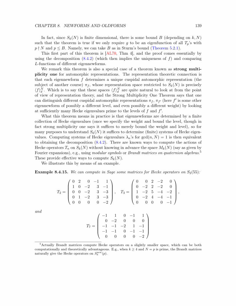
CHAPTER 8. NEWFORMS AND OLDFORMS 139
In fact, since Sk(N) is finite dimensional, there is some bound B (depending on k,N)such that the theorem is true if we only require g to be an eigenfunction of all Tp’s withp - N and p ≤ B. Namely, we can take B as in Sturm’s bound (Theorem 5.2.1).
This first part of this theorem is [AL70, Thm 4], and the proof comes essentially byusing the decomposition (8.4.2) (which then implies the uniqueness of f) and comparingL-functions of different eigennewforms.
We remark this theorem is also a special case of a theorem known as strong multi-plicity one for automorphic representations. The representation theoretic connection isthat each eigennewform f determines a unique cuspidal automorphic representation (thesubject of another course) πf , whose representation space restricted to Sk(N) is precisely〈f〉Nd . Which is to say that these spaces 〈f〉Nd are quite natural to look at from the pointof view of representation theory, and the Strong Multiplicity One Theorem says that onecan distinguish different cuspidal automorphic representations πf , πf ′ (here f ′ is some othereigennewform of possibly a different level, and even possibly a different weight) by lookingat sufficiently many Hecke eigenvalues prime to the levels of f and f ′.
What this theorem means in practice is that eigennewforms are determined by a finitecollection of Hecke eigenvalues (once we specify the weight and bound the level, though infact strong multiplicity one says it suffices to merely bound the weight and level), so formany purposes to understand Sk(N) it suffices to determine (finite) systems of Hecke eigen-values. Computing systems of Hecke eigenvalues λn’s for gcd(n,N) = 1 is then equivalentto obtaining the decomposition (8.4.2). There are known ways to compute the actions ofHecke operators Tn on Sk(N) without knowing in advance the spaceMk(N) (say as given byFourier expansions), e.g., using modular symbols or Brandt matrices on quaternion algebras.5
These provide effective ways to compute Sk(N).We illustrate this by means of an example.
Example 8.4.15. We can compute in Sage some matrices for Hecke operators on S2(55):
T2 =
0 2 0 −1 11 0 −2 3 −10 0 −2 3 −30 1 −2 3 −30 0 0 0 −2
, T3 =
0 0 2 −2 00 −2 2 −2 01 −2 5 −4 −20 −2 4 −4 −10 0 0 0 −1
,
and
T7 =
−1 1 0 −1 1
0 −2 0 0 0−1 −1 −2 1 −1−1 −1 0 −1 −1
0 0 0 0 −2
5Actually Brandt matrices compute Hecke operators on a slightly smaller space, which can be both
computationally and theoretically advantageous. E.g., when k ≥ 4 and N = p is prime, the Brandt matricesnaturally give the Hecke operators on Snew
k (p).
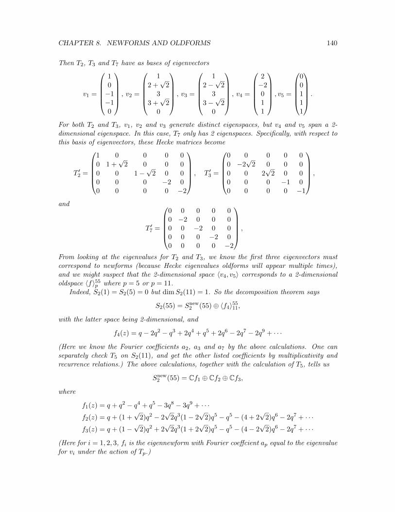
CHAPTER 8. NEWFORMS AND OLDFORMS 140
Then T2, T3 and T7 have as bases of eigenvectors
v1 =
10−1−10
, v2 =
1
2 +√
23
3 +√
20
, v3 =
1
2−√
23
3−√
20
, v4 =
2−2011
, v5 =
00111
.
For both T2 and T3, v1, v2 and v3 generate distinct eigenspaces, but v4 and v5 span a 2-dimensional eigenspace. In this case, T7 only has 2 eigenspaces. Specifically, with respect tothis basis of eigenvectors, these Hecke matrices become
T ′2 =
1 0 0 0 0
0 1 +√
2 0 0 0
0 0 1−√
2 0 00 0 0 −2 00 0 0 0 −2
, T ′3 =
0 0 0 0 0
0 −2√
2 0 0 0
0 0 2√
2 0 00 0 0 −1 00 0 0 0 −1
,
and
T ′7 =
0 0 0 0 00 −2 0 0 00 0 −2 0 00 0 0 −2 00 0 0 0 −2
,
From looking at the eigenvalues for T2 and T3, we know the first three eigenvectors mustcorrespond to newforms (because Hecke eigenvalues oldforms will appear multiple times),and we might suspect that the 2-dimensional space 〈v4, v5〉 corresponds to a 2-dimensionaloldspace 〈f〉55
p where p = 5 or p = 11.Indeed, S2(1) = S2(5) = 0 but dimS2(11) = 1. So the decomposition theorem says
S2(55) = Snew2 (55)⊕ 〈f4〉55
11,
with the latter space being 2-dimensional, and
f4(z) = q − 2q2 − q3 + 2q4 + q5 + 2q6 − 2q7 − 2q9 + · · ·
(Here we know the Fourier coefficients a2, a3 and a7 by the above calculations. One canseparately check T5 on S2(11), and get the other listed coefficients by multiplicativity andrecurrence relations.) The above calculations, together with the calculation of T5, tells us
Snew2 (55) = Cf1 ⊕ Cf2 ⊕ Cf3,
where
f1(z) = q + q2 − q4 + q5 − 3q8 − 3q9 + · · ·f2(z) = q + (1 +
√2)q2 − 2
√2q3(1− 2
√2)q5 − q5 − (4 + 2
√2)q6 − 2q7 + · · ·
f3(z) = q + (1−√
2)q2 + 2√
2q3(1 + 2√
2)q5 − q5 − (4− 2√
2)q6 − 2q7 + · · ·
(Here for i = 1, 2, 3, fi is the eigennewform with Fourier coeffcient ap equal to the eigenvaluefor vi under the action of Tp.)

CHAPTER 8. NEWFORMS AND OLDFORMS 141
Let us end with some remarks on the original question about whetherMk(N) has a basisconsisting of forms whose Fourier coefficients are multiplicative for all n (i.e., amn = amanwhenever gcd(m,n) = 1).
By (8.4.2), for the space of cusp forms Sk(N), this boils down to determining whether,for every newform f ∈ Snew
k (d), the subspace Vf,m := 〈ιm(f) : m|Nd 〉 has a basis consistingof forms with multiplicative coefficients. As in Example 8.4.11, we expect this to be true forSk(p) because conjecturally there is a basis of complete eigenforms.
On the other hand, the Atkin–Lehner decomposition easily gives a positive answer to amore generalized notion of multiplicative coefficients:
Proposition 8.4.16. The space Sk(N) has a basis of forms f(z) =∑anq
n whose Fouriercoefficients are essentially multiplicative in the following sense: for each such f , there existsm ∈ N (in fact m|N) such that an = 0 if m - n and amnn′ = amnamn′ for all n, n′ ∈ N suchthat gcd(n, n′) = 1.
Note that the essential multiplicativity condition is simply multiplicativity when m = 1.
Proof. Note ιm(f) satisfies this property for a newform f ∈ Sk(d), and apply the decompo-sition (8.4.2).
If one wants to extend this to Mk(N), one needs a newform theory for Eisenstein series.This was not done by Atkin and Lehner, but worked out in the thesis of Weisinger (Harvard,1977). We won’t explain this, but just mention it is possible. The obstruction to definingnewforms in Mk(N) in the same way as for Sk(N) is that the Petersson inner product is notdefined on all of Mk(N).

Chapter 9
Hilbert modular forms
The modular forms we have been studying up until now are often called elliptic modularforms, due to the connection with classical elliptic functions (and elliptic curves). In thischapter, we give a brief exposition of the theory of Hilbert modular forms, which is one kindof generalization of our usual elliptic modular forms. We will assume some familiarity withbasic algebraic number theory in this chapter.
We motivated the theory of modular forms in the introduction via quadratic formsand theta series. Namely, the number of ways rk(n) is a sum of k-squares is just the n-th coefficient in the q-expansion of ϑk(z). Observing that ϑ satisfies some transformationproperties, we consider the space of functions with similar properties, and are led to the thedefinition of a modular form of weight k/2.
One can similarly motivate the theory of Hilbert modular forms by considering quadraticforms over more general number fields. For simplicity, suppose F = Q(
√d) is with d > 0
the discriminant and having class number one. This has ring of integers OF = Z[√d] if
d ≡ 0 mod 4 and OF = Z[1+√d
2 ] if d ≡ 1 mod 4. Here the right analogue of Jacobi’s thetafunction from (4.4.1) is
ϑOF (z1, z2) =∑
a+b√d∈OF
e2πi(z1(a+b√d)2+z2(a−b
√d)2) =
∑α∈OF
qα2
1 qα2
2 ,
where qi = e2πizi . The reason one considers a theta function of 2 variables is to account forthe two embeddings of F into R. Note this contains the more naive generalization∑
α∈OF
qα2
= ϑOF (z, 0)
of Jacobi’s theta function, where, as usual q = e2πiz. However, one gets a nicer theory byaccounting for the different embedding of F into R (just as one does in algebraic numbertheory). Using ϑOF , one can study the number of representations of n in OF as a sum of ksquares. Again, one can proceed from the transformation properties of ϑOF to define Hilbertmodular forms over F . Notice that our “Fourier expansion” is also more complicated in thiscase—it runs not over Z but over OF .
While quadratic forms provided our main motivating problem to study modular forms,we built up the definition more geometrically, by considering the surfaces Y0(N) = Γ0(N)\H
142
CHAPTER 9. HILBERT MODULAR FORMS 143
(or rather their compactifications X0(N)) and studying functions on them. Recall thatwhile there are no nonconstant holomorphic functions on X0(N), the derivatives of modu-lar functions (weak modular forms) have different transformation properties and for mosteven weights (just exclude k = 2 when N = 1), there are non-constant holomorphic forms.Consequently one can construct modular functions by constructing holomorphic modularforms and taking appropriate products and ratios to get something of weight 0 (a mod-ular function). This gives a construction of the famous j-invariant modular function inExercise 4.2.13, which is important in the theory of elliptic curves.1
In our real quadratic case F = Q(√d), the analogue will be to look at functions on a
quotient Γ\(H× H), where Γ is a group of isometries of H× H. Note that since PSL2(R) isthe isometry group of H, PSL2(R)×PSL2(R) acts by isometries on H×H. The embeddingα 7→ (α, α) of F into R × R that one usually considers in algebraic number theory inducesan embedding of PSL2(F ) into PSL2(R)×PSL2(R). The analogue of looking at congruencesubgroups of PSL2(Z) in the case of modular forms is to look at congruence subgroups
Γ ⊂ PSL2(OF ) ⊂ PSL2(R)× PSL2(R).
In fact one often replaces PSL2(OF ) by slightly more general arithmetic groups.Either of these approaches lead one to define Hilbert modular forms over a totally real
number field F (i.e., all embeddings of F into C lie in R, so Q( 3√
2) is real, but not totallyreal).
Hilbert’s motivation for studying modular forms over number fields was as follows. TheKronecker–Weber theorem says that any abelian extension of Q can be generated by rootsof unity, i.e., special values of the function f(x) = eix. The theory of complex multiplicationdoes something analogous for imaginary quadratic extensions K/Q, realizing Kronecker’sJugendtraum (“dream of youth”). Specifically, one can generate any abelian extension of Kusing special values of the j-invariant special values of the Weierstrass ℘ function. Hilbert’stwelfth problem asks more generally for a determination of the the abelian extensions ofa general number field K. Consequently, one wants analogues of special functions likeexponential functions, the modular function j(τ) and the ℘ function. Hilbert’s idea was toconsider modular forms over number fields to find analogues of these special functions.
Some references are [Fre90] for full level, [Bru08] or [vdG88] for F real quadratic, or[Gar90] or [Shi78] in full generality.
9.1 Basic definitions and results
Let F be a totally real number field of degree r, i.e., [F : Q] = r and there are r embeddings,ι1, . . . , ιr, of F into R. Denote the ring of integers of F by OF . We consider all of theseembeddings at once via
ι : F → Rr, ι(x) = (ι1(x), . . . , ιr(x)).
1In retrospect, I suppose this was a bit incoherent—our motivation for modular forms was to studyquadratic forms, and we use modular functions as motivation for the definition, but then we essentially dropthe problem of constructing modular functions once we have the definition of modular forms apart from thatone exercise, and just study modular forms with applications to quadratic forms. If I ever add a chapter onelliptic curves, I will hopefully say more about the j-invariant so that there is some payoff of spending allthat time on modular functions.

CHAPTER 9. HILBERT MODULAR FORMS 144
The advantage of doing this is that then ι(OF ) is a lattice (discrete Z-module) in Rr, which isanalogous to Z being a discrete subgroup of R. (Note if we just consider a single embedding,e.g., Z[
√5] ⊂ R, we do not get a discrete subset of R when r > 1.)
Elliptic modular forms arose from looking at the modular curves Γ\H, where Γ is afinite-index subgroup of PSL2(Z), which acts discretely on H (i.e., the orbits under thisaction are discrete subsets of H). The analogue should be to look at finite-index subgroupsof PSL2(OF ). But since PSL2(OF ) ⊂ PSL2(R) does not act discretely on H. Just as OF canbe viewed as a lattice in Rr, we can view PSL2(OF ) acting discretely on the r-fold productof upper-half planes Hr.
For g = (g1, . . . , gr) ∈ PSL2(R)r, we let g act on Hr via
g · z = (g1z1, . . . , grzr), z = (z1, . . . , zr).
Then we extend
ι : GL2(F )→ GL2(R)r, ι(γ) = (ι1(γ), . . . , ιr(γ)),
whereιi(γ) : GL2(F )→ GL2(R) is just given by coordinate-wise application of ιi. Restrictingto SL2(F ) and quotienting out by ±I gives gives an embedding ι : PSL2(F )→ PSL2(R)r. So
we let PSL2(F ) act on Hr via composition with ι. Notationally, if γ =
(a bc d
)∈ PSL2(F )
and z = (z1, . . . , zr), we will denote this action by(a bc d
)z =
az + b
cz + d:=
(ι1(a)z1 + ι1(b)
ι1(c)z1 + ι1(d), . . . ,
ιr(a)z1 + ιr(b)
ιr(c)z1 + ιr(d)
).
Proposition 9.1.1. PSL2(OF ) acts discretely on Hr.
We call PSL2(OF ) the (full) Hilbert modular group. The analogue of the congruencesubgroups Γ0(N) inside PSL2(Z) are
Γ0(N) =
(a bc d
)∈ SL2(OF ) : c ∈ N
/ ±I ,
where N is a nonzero integral ideal of OF . We call these congruence subgroups ofPSL2(OF ). (As when r = 1, there are more congruence subgroups than just the Γ0(N)’s,but these are all we will consirer.) Note when F = Q, Γ0(NZ) = Γ0(N) for N ∈ N. Ingeneral, one can check that Γ0(N) has finite index in PSL2(OF ).
As in the case of r = 1, one adjoins cusps to Hr. Namely, we define the extended r-foldproduct of upper half-planes Hr to be the union of Hr together with the boundary pointsι(F ) ⊂ Rr and the point at infinity i∞ = (i∞, . . . , i∞). Then Hr ⊂ H ∪ R ∪ i∞r. Theelements of Hr − Hr are the cusps of Hr. There is a natural way to put a topology on Hr
as well as extend the action of PSL2(F ) to Hr. Thus for a subgroup Γ of PSL2(OF ), we cantalk about the cusps of the quotient Γ\Hr, which are the Γ-orbits of the cusps of Hr.
Unlike the case of F = Q, there may be many cusps for PSL2(OF )\Hr, but one can showthere are finitely many:
Theorem 9.1.2. The number of cusps of PSL2(OF )\Hr is the class number hF of F .
CHAPTER 9. HILBERT MODULAR FORMS 145
For c, d ∈ F , k ∈ Zr and z = (z1, . . . , zr) ∈ Hr, we denote by
(cz + d)k = (ι1(c)z1 + ι1(d))k1 · · · (ιr(c)z1 + ιr(d))kr .
Definition 9.1.3. Let k = (k1, . . . , kr) ∈ Zr and Γ be a finite index subgroup of PSL2(OF ).A (holomorphic) Hilbert modular form of weight k on Γ\Hr is holomorphic* functionf : Hr → C satisfying
f(γz) = (cz + d)kf(z), γ =
(a bc d
)∈ Γ0(N). (9.1.1)
If also f vanishes at the cusps, we say f is a cusp form. Denote the space of weight kHilbert modular forms and cusp forms on Γ\Hr respectively by Mk(Γ) and Sk(Γ).
If Γ = Γ0(N), then we write Mk(N) = Mk(Γ) and Sk(N) = Sk(Γ). A form in Mk(N)is said to have level N.
For F = Q, we have Mk(NZ) = Mk(N) and Sk(NZ) = Sk(N). When F 6= Q, by aholomorphic function of Hr we mean a function f : Hr → C which is holomorphic in each ofthe r complex variables z1, . . . , zr. It should also extend to be “holomorphic at the cusps,”which is a notion one can define precisely, and once one defines it one can show it’s notactually needed! (That is, it’s not needed for the definition of holomorphic Hilbert modularforms, but it is used in the theory.)
Theorem 9.1.4. (Koecher’s principle) Suppose [F : Q] > 1. If f : Hr → C is holomor-phic and satisfies (9.1.1), then f is holomorphic at the cusps.
The proof of Koecher’s principle uses Fourier expansions, which we describe next (thatis, we describe Fourier expansions, but not the proof of Koecher’s principle).
The inverse different of F is the fractional ideal
O⊥F =x ∈ F : trF/Q(xOF ) ⊂ OF
.
Here the trace from F to Q is defined as the sum of the conjugates, i.e., trF/Q(x) =∑ιi(x).
So if we define tr : Cr → C via tr(z1, . . . , zr) =∑zi, then tr(ι(x)) = trF/Q(x), which we
also denote simply as tr(x).
Proposition 9.1.5. Given f ∈Mk(N), we have the Fourier expansion (at ∞)
f(z) =∑ξ∈O⊥F
cξe2πitr(ξz) =
∑ξ∈O⊥F
cξe2πi(ι1(ξ)z1+···+ιr(ξ)zr),
for some (uniquely determined) collection of Fourier coefficients cξ ∈ C.
As when F = Q, there are also Fourier expansions around other cusps.To specify f , we sometimes denote the Fourier coefficient cξ by cξ(f). The idea of the
proof is to use that fact that f is invariant under action by(
1 x0 1
)for all x ∈ OF .
We call x ∈ F totally positive if ιi(x) > 0 for all x. Koecher’s principle in fact tells us:

CHAPTER 9. HILBERT MODULAR FORMS 146
Theorem 9.1.6. (Koecher’s principle, 2nd version) For f ∈Mk(N), cξ(f) = 0 unlessξ = 0 or ξ is totally positive.
As in the case of F = Q, a necessary condition for f to be a cusp form is c0(f) = 0.
Corollary 9.1.7. Let f ∈Mk(N), where k = (k1, . . . , kr). If some ki 6= kj, then f ∈ Sk(N).
We call the weight of the form k = (k, . . . , k) parallel weight k. Thus the corollarytells us that we can only have non-cuspidal holomorphic Hilbert modular forms (e.g., theEisenstein series discussed below) in parallel weights. Another nice thing about parallelweights is restriction to the diagonal yields elliptic modular forms:
Exercise 9.1.8. Let f ∈ Mk(NOF ) where N ∈ N and k = (k, . . . , k). Show g : H → Cgiven by g(z) = f(z, . . . , z) is an elliptic modular form in Mk(N).
Theorem 9.1.9. dimMk(N) <∞.

Bibliography
[Ahl78] Lars V. Ahlfors, Complex analysis, third ed., McGraw-Hill Book Co., New York,1978, An introduction to the theory of analytic functions of one complex variable,International Series in Pure and Applied Mathematics. MR 510197 (80c:30001)
[AL70] A. O. L. Atkin and J. Lehner, Hecke operators on Γ0(m), Math. Ann. 185 (1970),134–160. MR 0268123 (42 #3022)
[And05] James W. Anderson, Hyperbolic geometry, second ed., Springer UndergraduateMathematics Series, Springer-Verlag London Ltd., London, 2005. MR 2161463(2006b:51001)
[Apo90] Tom M. Apostol, Modular functions and Dirichlet series in number theory, seconded., Graduate Texts in Mathematics, vol. 41, Springer-Verlag, New York, 1990.MR 1027834 (90j:11001)
[Boy01] Matthew Boylan, Swinnerton-Dyer type congruences for certain Eisenstein series,q-series with applications to combinatorics, number theory, and physics (Urbana,IL, 2000), Contemp. Math., vol. 291, Amer. Math. Soc., Providence, RI, 2001,pp. 93–108. MR 1874523 (2002k:11063)
[Bru08] Jan Hendrik Bruinier, Hilbert modular forms and their applications, The 1-2-3 ofmodular forms, Universitext, Springer, Berlin, 2008, pp. 105–179. MR 2447162
[Bum97] Daniel Bump, Automorphic forms and representations, Cambridge Studies in Ad-vanced Mathematics, vol. 55, Cambridge University Press, Cambridge, 1997. MR1431508 (97k:11080)
[CSS97] Gary Cornell, Joseph H. Silverman, and Glenn Stevens (eds.), Modular formsand Fermat’s last theorem, Springer-Verlag, New York, 1997, Papers from theInstructional Conference on Number Theory and Arithmetic Geometry held atBoston University, Boston, MA, August 9–18, 1995. MR 1638473 (99k:11004)
[DS05] Fred Diamond and Jerry Shurman, A first course in modular forms, GraduateTexts in Mathematics, vol. 228, Springer-Verlag, New York, 2005. MR 2112196(2006f:11045)
[Els06] Jürgen Elstrodt, A very simple proof of the eta transformation formula,Manuscripta Math. 121 (2006), no. 4, 457–459. MR 2283473 (2007g:11051)
147

BIBLIOGRAPHY 148
[FB09] Eberhard Freitag and Rolf Busam, Complex analysis, second ed., Universitext,Springer-Verlag, Berlin, 2009. MR 2513384
[Fre90] Eberhard Freitag, Hilbert modular forms, Springer-Verlag, Berlin, 1990. MR1050763
[Gar90] Paul B. Garrett, Holomorphic Hilbert modular forms, The Wadsworth &Brooks/Cole Mathematics Series, Wadsworth & Brooks/Cole Advanced Books &Software, Pacific Grove, CA, 1990. MR 1008244
[Iwa97] Henryk Iwaniec, Topics in classical automorphic forms, Graduate Studies in Math-ematics, vol. 17, American Mathematical Society, Providence, RI, 1997. MR1474964 (98e:11051)
[Kat92] Svetlana Katok, Fuchsian groups, Chicago Lectures in Mathematics, University ofChicago Press, Chicago, IL, 1992. MR 1177168 (93d:20088)
[Kil08] L. J. P. Kilford, Modular forms, Imperial College Press, London, 2008, A classicaland computational introduction. MR 2441106 (2009m:11001)
[KL06] Andrew Knightly and Charles Li, Traces of Hecke operators, Mathematical Surveysand Monographs, vol. 133, American Mathematical Society, Providence, RI, 2006.MR 2273356
[Kob93] Neal Koblitz, Introduction to elliptic curves and modular forms, second ed., Grad-uate Texts in Mathematics, vol. 97, Springer-Verlag, New York, 1993. MR 1216136(94a:11078)
[Lan95] Serge Lang, Introduction to modular forms, Grundlehren der Mathematischen Wis-senschaften [Fundamental Principles of Mathematical Sciences], vol. 222, Springer-Verlag, Berlin, 1995, With appendixes by D. Zagier and Walter Feit, Correctedreprint of the 1976 original. MR 1363488 (96g:11037)
[Lan99] , Complex analysis, fourth ed., Graduate Texts in Mathematics, vol. 103,Springer-Verlag, New York, 1999. MR 1659317 (99i:30001)
[Mar05] Greg Martin, Dimensions of the spaces of cusp forms and newforms on Γ0(N) andΓ1(N), J. Number Theory 112 (2005), no. 2, 298–331. MR 2141534
[Mil] J.S. Milne, Modular functions and modular forms, Online course notes.http://www.jmilne.org/math/CourseNotes/mf.html.
[Miy06] Toshitsune Miyake, Modular forms, english ed., Springer Monographs in Mathe-matics, Springer-Verlag, Berlin, 2006, Translated from the 1976 Japanese originalby Yoshitaka Maeda. MR 2194815 (2006g:11084)
[Sch74] Bruno Schoeneberg, Elliptic modular functions: an introduction, Springer-Verlag,New York, 1974, Translated from the German by J. R. Smart and E. A. Schwandt,Die Grundlehren der mathematischen Wissenschaften, Band 203. MR 0412107 (54#236)

BIBLIOGRAPHY 149
[Ser73] J.-P. Serre, A course in arithmetic, Springer-Verlag, New York, 1973, Translatedfrom the French, Graduate Texts in Mathematics, No. 7. MR 0344216 (49 #8956)
[Shi78] Goro Shimura, The special values of the zeta functions associated with Hilbertmodular forms, Duke Math. J. 45 (1978), no. 3, 637–679. MR 507462
[Sta09] John Stalker, Complex analysis, Modern Birkhäuser Classics, Birkhäuser BostonInc., Boston, MA, 2009, Fundamentals of the classical theory of functions, Reprintof the 1998 edition. MR 2547082 (2010i:30001)
[Ste07] William Stein, Modular forms, a computational approach, Graduate Studies inMathematics, vol. 79, American Mathematical Society, Providence, RI, 2007, Withan appendix by Paul E. Gunnells. MR 2289048 (2008d:11037)
[vdG88] Gerard van der Geer, Hilbert modular surfaces, Ergebnisse der Mathematik undihrer Grenzgebiete (3) [Results in Mathematics and Related Areas (3)], vol. 16,Springer-Verlag, Berlin, 1988. MR 930101
[Zag08] Don Zagier, Elliptic modular forms and their applications, The 1-2-3 of modularforms, Universitext, Springer, Berlin, 2008, pp. 1–103. MR 2409678 (2010b:11047)

Index
Bk, 56E(Λ), 21Ek, 53Ek,N , 53Gk, 55Gk,N , 58L(s, χ), 115L(s, f), 120Mk(N), 145Mk(N), 63Mk(Γ), 63S, 31Sk(N), 145Sk(N), 75Sk(Γ), 75T , 31Tn, 98, 128Up, 129Wp, 134Y0(N), 44Z(s), 114〈f, g〉, 108∆(z), 76Γ(N), 36Γ0(N), 36Γ1(N), 36H, 24, 26Λ(s, f), 120PSL2(R), 28SL2(R), 28H, 41f , 120δk(n), 71η(z), 72C, 15P1(Z/NZ), 36σk(m), 56
τ(n), 76ϑ(z), 67℘, 22ζ(s), 113cξ(f), 145j-invariant, 57j(γ, z), 51p(n), 74q-expansion, 45, 46qN , 46qτ , 46vp(f), 79
analytic, 13Atkin–Lehner operator, 134automorphy factor, 51
Bernoulli number, 56
Cauchy’s residue theorem, 78Cauchy–Riemann equations, 12completed L-function, 120completed zeta function, 114congruence subgroup, 36, 144critical line, 114critical strip, 114cusp, 144cusp form, 75cusps, 41
Dedekind eta function, 72Dedekind zeta function, 117degree, 118dimension formula, 86Dirichlet L-function, 115Dirichlet character, 115Dirichlet convolution, 132discriminant, 23
150

INDEX 151
discriminant modular form, 76
eigenform, 102, 129eigennewform, 136Eisenstein series, 52elliptic curve, 23elliptic element, 39elliptic function, 21elliptic modular form, 142elliptic point, 39entire, 12equivalent (lattices), 24Euler product, 115explicit formula, 114extended upper half-plane, 41
Fourier coefficient, 19, 145Fourier coefficients, 63Fourier expansion, 46, 145fractional linear transformation, 28Fricke involution, 120, 134functional equation, 114fundamental domain, 18, 32
gamma function, 114
Hecke L-function, 120Hecke converse theorem, 121Hecke operator, 98, 127Hilbert cusp form, 145Hilbert modular form, 145Hilbert modular group, 144holomorphic, 12holomorphic at i∞, 62holomorphic at cusps, 62hyperbolic plane, 26
inverse different, 145
Jacobi theta function, 67
Koecher’s principle, 145, 146
Laurent series, 15level, 50, 63, 145Lipschitz’ formula, 54local L-factor, 118
Möbius inversion, 60Maass form, 106Mellin transform, 121meromorphic, 15meromorphic at ∞, 20meromorphic at cusps, 62meromorphic modular form, 63moderate growth, 48modular curve, 44modular form, 63modular function, 45, 47modular group, 31, 36multiplicative, 118
newform, 136
oldform, 136open mapping theorem, 49order, 79order (of elliptic point), 40order (of pole), 15order (of zero), 14
parallel weight, 146pentagonal number, 73Petersson inner product, 108principal congruence subgroup, 36projective line, 36projective special linear group, 28
Ramanujan tau function, 76residue, 78Riemann sphere, 15Riemann zeta function, 113
slash operator, 46, 62, 97special linear group, 28standard fundamental domain, 34Sturm’s bound, 88
totally multiplicative, 118totally positive, 145trace, 145triangular number, 71
upper half-plane, 24, 26
weak modular form, 50
INDEX 152
Weierstrass form, 23Weierstrass pe, 22weight, 50, 145
Recommended

![Computing power series expansions of modular forms · Computing power series expansions of modular forms 3 modular forms. Mori [29, 30] and Datskovsky and Guerzhoy [14] have also](https://img.pdfslide.net/doc/110x75/5ec388a12d0af455e7148f76/computing-power-series-expansions-of-modular-forms-computing-power-series-expansions.jpg)


![[Tutorial] Modular Forms - PARI/GP · Modular forms attached toHecke characterson imaginary and real quadratic fields. Modular forms associated toelliptic curvesby Wiles’s modularity](https://img.pdfslide.net/doc/110x75/5f5af59a26f27b13500199d4/tutorial-modular-forms-parigp-modular-forms-attached-tohecke-characterson-imaginary.jpg)
![SPECTRAL HALO FOR HILBERT MODULAR FORMS · The theory of p-adic analytic families of modular forms grew out of the study of congru-ences of modular forms. In [22], Serre gave the](https://img.pdfslide.net/doc/110x75/5f16a4b8d7c9c12d882bf82f/spectral-halo-for-hilbert-modular-forms-the-theory-of-p-adic-analytic-families-of.jpg)


![Modular Forms and Modular Congruences of the Partition ...abel.harvard.edu/theses/senior/narayanan/narayanan.pdf · [11]. Modular forms have also proven useful in understanding sphere](https://img.pdfslide.net/doc/110x75/5f0ccd9c7e708231d4373551/modular-forms-and-modular-congruences-of-the-partition-abel-11-modular-forms.jpg)