1
Monopolistic Competition and Macroeconomic Dynamics
Pasquale Commendatore, Università di Napoli ‘Federico II’
Ingrid Kubin, Vienna University of Economics and Business Administration
Abstract
Modern macroeconomic models with a Keynesian flavor usually involve nominal rigidities
in wages and commodity prices. A typical model is static and combines wage bargaining in
the labor markets and monopolistic competition in the commodity markets. As central
policy implication follows that deregulating labor and/or commodity markets increases
equilibrium employment.
We reassess the consequences of deregulation in a dynamic model. It still increases
employment at the fixed point, which corresponds to the static equilibrium solution.
However, the fixed point loses stability through a Flip-bifurcation with stronger
deregulation; numerical simulations illustrate that deregulation may even reduce average
employment.
JEL: E1
Corresponding author:
Ingrid Kubin
University of Economics and
Business Administration – VWL7 e-mail: [email protected]
Augasse 2-6 Tel.: +43 31336 4456
A-1090 Vienna, Austria Fax: +43 31336 9209
2
1. Introduction1
Modern macroeconomic models with a Keynesian flavor usually involve nominal rigidities
in wages and/or commodity prices (see Gordon, 1990). A typical microfoundation for the
latter recurs to the Dixit-Stiglitz model of monopolistic competition (Dixit and Stiglitz,
1977). Keynesian features studied in such models are the possibility of unemployment (e.g.
d’Aspremont et al., 1990) and multiple equilibria (e.g. d’Aspremont et al., 1995,
Linnemann, 2001) and that fiscal policy has income multiplier effects (Heijdra and
Ligthart, 1997; Heijdra et al., 1998; see also Solow, 1998). Blanchard and Kiyotaki (1987)
proposed a prototype macro-model combining monopolistic competition in the commodity
markets with labor market imperfections that has now become a standard framework for
analyzing unemployment problems. The widely used approach of specifying a wage setting
and a price setting equation (see e.g. Nickel, 1990; Layard et al., 1991; or Blanchard, 2003;
and for empirical applications various analyses by the European Commission, e.g.
McMorrow and Roeger, 2000; Bains et al., 2002) ultimately rests upon such micro
foundations. Blanchard and Giavazzi (2001) recently presented a structural model along
these lines combing monopolistic competition with wage bargaining (similar also Jerger,
2001, in an open economy context). A characteristic result in those analyses is that
deregulating the labor markets (i.e. reducing the bargaining power of workers and/or
reducing the unemployment benefits) and/or deregulating the commodity markets (i.e.
1 An earlier version of the paper was presented at Workshops in Naples, Aix, Vienna and
Helsinki. We would like to thank Ulrich Berger, Peter Flaschel, Leo Kaas, Carlo Panico,
Florian Wagener and participants of the Workshops for helpful comments. The usual caveat
applies.
3
reducing the market power of commodity suppliers) increases equilibrium employment (see
also Gersbach, 1999 and 2000).
However, those models are typically static models, which do not specify explicitly the
economic process in time. In the following paper, we develop a dynamic macroeconomic
model in which commodity markets are characterized by monopolistic competition and
labor markets by wage bargaining.
In our analysis, the usual equilibrium solution is a fixed point of the dynamic model, which
exhibits the usual comparative static properties (deregulating the labor and/or the
commodity market increases employment). However, depending upon the parameters the
fixed point may lose stability through a Flip-bifurcation giving rise to cyclical solutions and
endogenous fluctuations. We show analytically that commodity and labor market
deregulation may lead to instability; in numerical simulations, we even found cases in
which deregulation leads to lower average employment. Both results, valid in a dynamic
framework, contrast with the usual comparative static properties.
The paper is organized as follows: In the second section, we present our model; its basic
structure closely follows Blanchard and Giavazzi (2001). Monopolistically competitive
firms bargain with unions over employment and nominal wage rates on the basis of firms’
anticipated demand functions and workers’ nominal reservation wages. In the third section,
we explicitly add two dynamic components. First, central to monopolistic competition is
that firms neglect the reactions of other firms. They therefore base their decisions on a too
high anticipated price elasticity; outside equilibrium, they are necessarily surprised by the
market results. As a consequence, they will adjust their anticipated demand function over
4
time2. Second, the nominal reservation wage also adjusts through time on the basis of the
realized employment and the realized nominal wage rate. Whereas for the second process
several plausible specifications do exist, the specification of the first one is directly implied
by the external effect at the core of the monopolistic competition model itself. We show
that the first process leads to diverging time paths: while it still holds that deregulation
increases stationary employment, it leads to fundamental instability. In the fourth section,
we study two different specifications for the reservation wage adjustment, each of which
mirrors a different institutional set up. We show analytically that this second process may
dampen the sharp instability result: deregulation may still destabilize the economy;
however, the time path does not diverge but is attracted to a period-two cycle or eventually
to a complex time path. Some simulations complete the dynamic explorations. The last
section is left for concluding remarks.
2. The economic frame work
The analysis, being framed in a dynamic setting, requires dealing explicitly with time. We
assume that during the time unit, which for expository purposes we call ‘Week t’, all events
occur according to a well-defined sequence. On Monday of Week t, firm i and the
associated union bargain over employment and the nominal wage rate on the basis of firms’
anticipated demand and workers’ nominal reservation wage. Production occurs during the
2 See Currie and Kubin (2002) for an exploration of the monopolistic competition
dynamics. D’Aspremont et al. (1995) analyze endogenous fluctuations in what they call a
Cournotian monopolistic competition model. In contrast to our approach, the dynamics in
their model is driven by an overlapping generations structure and variable mark-ups are
central for the occurrence of endogenous fluctuations.
5
Week from Tuesday to Friday. On Friday, commodities are delivered to the market. Market
equilibrium determines the realized price. Finally, on Saturday firms and unions update the
information relevant for decisions in the following period concerning the employment, the
nominal wage rate and the realized price.
2.1 Firms and Households
The economy comprises a fixed number m of firms, each firm producing one differentiated
good in a regime of monopolistic competition; and L households, which own the existing
firms, each household supplying one unit of labor. Each firm faces a union composed of
i
LM
m= members.
All firms share the same production technology, which involves only one input, labor, used
in a fixed proportion. Assuming that during Week t firm i employs tiN workers, the
production of good i is:
( )t t ti i ix f N N= = (1)
for i = 1 … m.
Following Blanchard and Giavazzi (2001), household j’s preferences towards good i (for
i = 1 … m and j = 1 … L) are represented by a CES utility function:
( )1 1 1
1
mt tj i
i
U m c
σσ σ
σ σ− −−
=
=
∑ (2)
where 1 < σ < ∞ is the elasticity of substitution between goods and tic is the consumption
level of good i for the period. Note that the inclusion of the factor 1σ
−m into the utility
function implies that the utility level depends only upon the overall consumption quantity
and not on the number of different consumption goods. This specification, therefore, does
6
not represent a preference for commodity variety and σ is a parameter related only to the
market power of a single commodity supplier (see Blanchard and Kiyotaki, 1987; and also
the discussion in Benassy, 1996). In Blanchard and Giavazzi (2001), it is the central
parameter for studying the effects of commodity market deregulation.
Household j’s demand for good i is given by
t
jt ij
t t
Y pd
mP P
σ−
=
where Yj is the household j’s nominal income and where
( )1
11
1
1 mt
t ii
P pm
σσ −−
=
=
∑ (3)
is a price index corresponding to the price of one unit of utility. Summing through j, we
obtain the demand for commodity i during Week t
ti
tt t
pYd
mP P
σ−
=
(4)
where Y is the overall nominal income of the economy. We neglect the Price Index Effect
and the Ford Effect (see Yang and Heijdra, 1993; Dixit and Stiglitz, 1993; and
d’Aspremont et al., 1990, 1996); the elasticity of demand with respect to the own price
therefore reduces to σ− .3
3 Linnemeier (2001) showed that both effects are at the root of a possible multiplicity of
equilibria. We prefer to demonstrate our results in the simplest possible framework with a
unique equilibrium.
7
If the price of each good is the same, ti tp p= , the price index becomes t tP p= and the
demand for an individual good simplifies to
tt
Yd
mp= (5)
In that case, the elasticity of demand with respect to the price is equal to 1− .
Moving on to the description of the events occurring during ‘Week t’, most of our
discussion will be devoted to the crucial ones, that is, the bargaining process and the
determination of the market equilibrium.
2.2 Bargaining
We employ the efficient bargaining model (McDonald and Solow, 1983; Layard and
Nickell, 1990): During the Monday of Week t the parties (firm i and the associated union)
bargain over employment and the nominal wage rate for the current period on the basis of a
known set of data relating to workers’ reservation wage and firm i’s anticipated demand
function. The solution maximizes the following Nash product
( ) ( )1t t t ti i i iZ Z
β βΠ Π
−− −
) ) (6)
where 0 < β < 1 represents the relative bargaining power of the unions, tiZ denotes the
value of the union’s objective function if an agreement is reached and tiΠ the
corresponding value for the firm. tiZ
) and t
iΠ)
are the respective va lues, if no contract is
concluded. We assume a utilitarian trade union. Observing that the CES indirect utility
function is given by the nominal income deflated by an expected price index tP% , the value
of the unions objective function is given by
( )t t t t
i i i i Rti
t
N W M N WZ
P
+ −= % (7)
8
where tiN denotes employment, t
iW the nominal wage rate and tRW the nominal reservation
wage, which indicates the income opportunities expected to prevail outside the firm under
consideration. With t
t i Ri
t
M WZ
P=
)% , the union’s contribution to the Nash bargain is
( )t
t t t tii i i R
t
NZ Z W W
P− = −
)% (8)
Turning now to the firm’s contribution, we note that all profits are distributed to the
owners’ households. Therefore, the firms’s objective is also defined in terms of the CES
indirect utility function. With 0Π =)
and using equation (1), it is thus given by
( )t t i t t
t t t ii i t i ii i i t
t t
p x W N Np W
P PΠ Π
−− = = −
) % %% % (9)
where tip% denotes the anticipated price for commodity i. The framework of the Dixit-
Stiglitz model of monopolistic competition suggests that the anticipated price is determined
along the following lines. Typically, each firm assumes that other firms will not react to its
own price decisions and that – when neglecting the Price Index effect and the Ford effect –
the price elasticity of their demand function is constant and equal to σ− . Therefore, a firm
that knows it sold in the previous period a quantity 1ˆ
−td at a price 1ˆ −tp will anticipate its
demand function for the current period to be given by:
( )
( ) ( )1 1
ˆ ˆ tt t i
tt ti i
d p Kd
p p
σ
σ σ− −= =%
% % (10)

9
where tiK is the position of the anticipated demand function. 4
Using equations (1) and (10) we obtain the anticipated price tip% as
1
t ti t
i
Kp
N
σ =
% (11)
We assume that this is common knowledge to both bargaining parties.
Efficient (Nash) bargaining between firm’s i and the associated union corresponds to
choosing tiN and t
iW so as to maximize the following expression subject to (11):
( ) ( ) ( ) ( )1 1 tt t t t t t t t ii i i i i R i i
t
NZ Z W W p W
P
β β β βΠ Π
− −− − = − −
) ) % % (12)
Observing that – consonant with the monopolistic competition set-up – the parties assume
the expected price index tP% to be independent of their decisions, the bargaining results in:
1
1t t
i RW Wσ β
σ− + = −
(13)
² 1 t ti RMR p W
σσ−
= =% (14)
1
t ti t RN K W
σσ
σ
− = −
(15)
Note the familiar result from the efficient bargaining problem, namely that a position is
chosen off the profit maximum. In equation (14), the marginal revenue is equated to the
4 In other words: Firms assume that they can sell the same quantity at the same price as in
the previous period and they assume that their quantity will react to a price change
according to an elasticity of σ− .
10
nominal reservation wage and not to the marginal cost (corresponding to the nominal wage
rate). It follows that the price is set as a mark-up over the reservation wage, ( )1t ti Rp Wµ= +% ,
where ( )1 1µ σ≡ − .
Following Blanchard and Giavazzi (2001), we interpret a decrease in the mark-up µ (i.e. an
increase in σ) as commodity market deregulation. It reduces the size of firm i’s anticipated
surplus per unit of output, ( )t t ti R Rp W Wµ− =% . Labor market deregulation is reflected in
Blanchard and Giavazzi (2001) by a decrease in the relative bargaining power of the union,
β . As equation (13) shows, β determines the distribution of the anticipated surplus between
wages and profits. Decreasing β reduces the workers’ share in the surplus, tRWβµ . In
addition, our model, as developed in the following sections, allows for labor market
deregulation in the form of changing the unemployment insurance scheme. This form of
labor market deregulation may also impinge on the bargaining outcome (and on the size of
the surplus) through its effects on the nominal reservation wage.
Note finally that equations (14) and (15) are not independent results, equation (15) can be
obtained from equation (14) by taking constraint (11) into account.
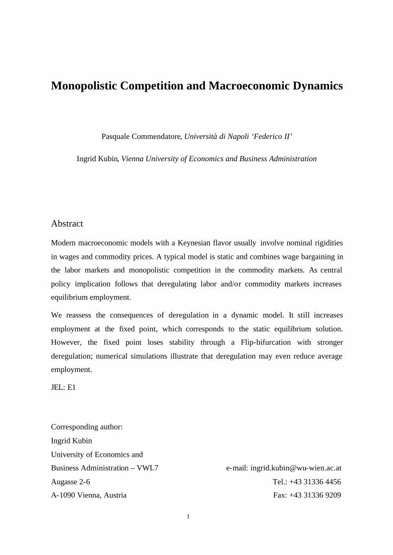
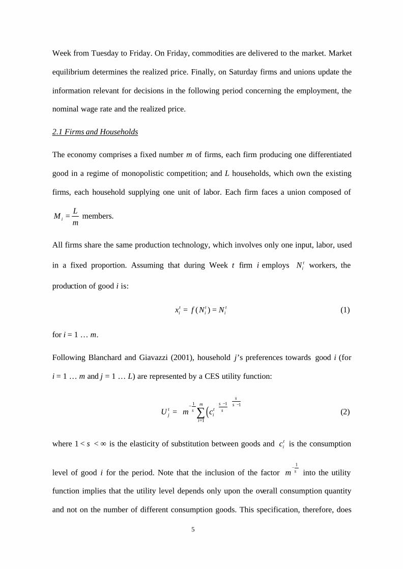
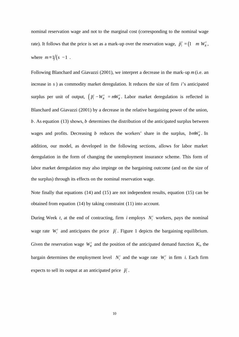
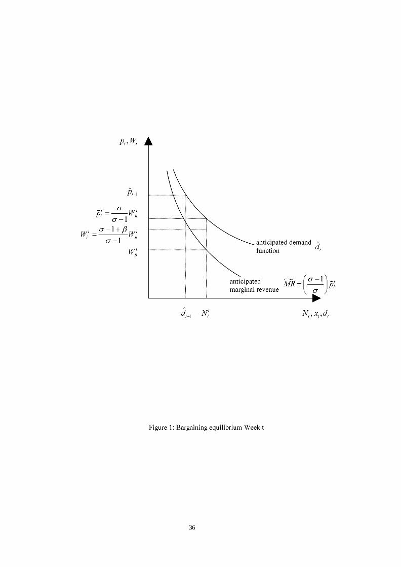
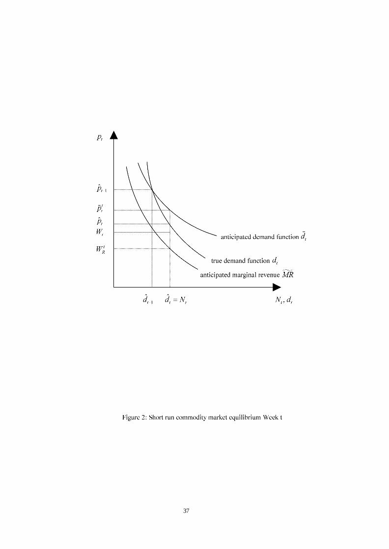
During Week t, at the end of contracting, firm i employs tiN workers, pays the nominal
wage rate tiW and anticipates the price t
ip% . Figure 1 depicts the bargaining equilibrium.
Given the reservation wage tRW and the position of the anticipated demand function Kt, the
bargain determines the employment level tiN and the wage rate t
iW in firm i. Each firm
expects to sell its output at an anticipated price % tip .

11
2.3 Short term commodity markets equilibrium
The characteristics of the commodity markets equilibrium follow from the assumption that
all firms behave identically – what Blanchard and Giavazzi (2001) call the symmetry
assumption. Each firm pays the same wage ti tW W= , hires the same number of workers,
ti tN N= , and produce the same quantity t
i tx x= , which is equal to their respective supplies
ti t ts s x= = . They envisage to sell these quantities at an identical anticipated price t t
ip p=% % .
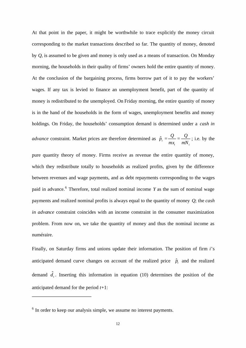
At the end of the production period, on Friday, each firm supplies st to the (identical) true
demand function dt (see Eq. (5)). In contrast to the anticipated demand functions, the true
demand functions take into account the reactions of all other firms; each of them has an
elasticity of 1− (instead of σ− ). Therefore, producers cannot realize their price and
quantity anticipations. In the following we assume that firms sell the entire quantity
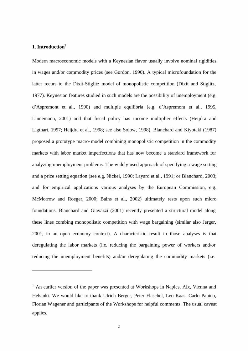
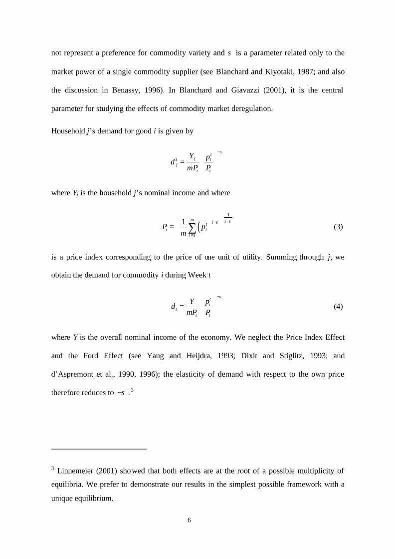
produced at the market-clearing price ˆtp (different from the anticipated price)5. Using (5),
the realized price is determined as:
t̂ t t td s x N= = = ˆtt t
Y Yp
mx mN= = (16)
Figure 2 depicts the short run commodity markets equilibrium.
5 In principle, producers as monopolists can also decide to sell a smaller quantity than the
produced one when entering the market. However, they do not have an incentive to do so:
On the basis of an elasticity of demand greater (anticipated demand) or equal to 1 (true
demand) in absolute terms, revenues do not increase with a quantity restriction. In addition,
at that moment, production costs are already sunk and maximizing revenues also
maximizes profits. Therefore, quantity restrictions cannot increase profits. Currie and
Kubin (2002) also explore an alternative quantity rationing scheme.
12
At that point in the paper, it might be worthwhile to trace explicitly the money circuit
corresponding to the market transactions described so far. The quantity of money, denoted
by Q, is assumed to be given and money is only used as a means of transaction. On Monday
morning, the households in their quality of firms’ owners hold the entire quantity of money.
At the conclusion of the bargaining process, firms borrow part of it to pay the workers’
wages. If any tax is levied to finance an unemployment benefit, part of the quantity of
money is redistributed to the unemployed. On Friday morning, the entire quantity of money
is in the hand of the households in the form of wages, unemployment benefits and money
holdings. On Friday, the households’ consumption demand is determined under a cash in
advance constraint. Market prices are therefore determined as ˆtt t
Q Qp
mx mN= = ; i.e. by the
pure quantity theory of money. Firms receive as revenue the entire quantity of money,
which they redistribute totally to households as realized profits, given by the difference
between revenues and wage payments, and as debt repayments corresponding to the wages
paid in advance.6 Therefore, total realized nominal income Y as the sum of nominal wage
payments and realized nominal profits is always equal to the quantity of money Q; the cash
in advance constraint coincides with an income constraint in the consumer maximization
problem. From now on, we take the quantity of money and thus the nominal income as
numéraire.
Finally, on Saturday firms and unions update their information. The position of firm i’s
anticipated demand curve changes on account of the realized price ˆtp and the realized
demand t̂d . Inserting this information in equation (10) determines the position of the
anticipated demand for the period t+1:
6 In order to keep our analysis simple, we assume no interest payments.
13
1ˆ ˆt t tK d pσ
+ = (17)
Similarly, workers’ reservation wage adjusts in the light of the realized nominal wage tW
and of the realized employment tN .
3. The dynamic system
3.1. Outline
The dynamic behavior of the model, therefore, involves two processes. First, since
producers do not know the true elasticity of the demand function, the position of the
anticipated demand function (and thus of the anticipated marginal revenue) shifts over time.
For a given nominal reservation wage and marginal revenue curve, the efficient bargaining
outcome, ² tRMR W= , determines employment. Since all firms are identical, equation (15)
can be written as:
1
tt t R
me K W
L
σσ
σ
− = −
(18)
where tt
mNe
L= denotes the employment rate. Taking into account equations (16) and (17),
it can also be written as
( )11 1
tt t R
Ye e W
L
σ σσσ σ
σ
−−−
− = −
(19)
Second, the nominal reservation wage, tRW , is also adjusted over time.
For expository purposes, in what follows we begin our study with the dynamics of the first
process in isolation by assuming a nominal reservation wage invariant over time. After that
14
we specify the adjustment of the reservation wage explicitly and explore the dynamic
properties of the full system.
3.2. Commodity market dynamics in isolation
If we assume a reservation wage fixed at an arbitrarily chosen level, tR RW W= , the implied
dynamic process is
( )11 1t t R
Ye e W
L
σ σσσ σ
σ
−−−
− = −
(20)
Equation (20) is a one-dimensional first-return map with the following fixed point and first
derivative
( )1
1
1 R
Ye W
Lσ
σ
−− = −
(21)
( ) ( ) 11
1 11
σ σσ σσ
σ σσ
−− −
−−
∂ = − = − ∂ −
FPt
R tt
e YW e
e L (22)
As long as σ > 1, the fixed point, given by equation (21), increases with σ,
0( 1)σ σ σ
∂= >
∂ −e e
, but loses stability at σ = 2. Eq. (22) shows that the derivative of the
first return map is negative for all values of the employment rate; therefore, the time path
diverges for σ > 2. Deregulating the commodity market increases the stationary
employment but may eventually lead to instability.
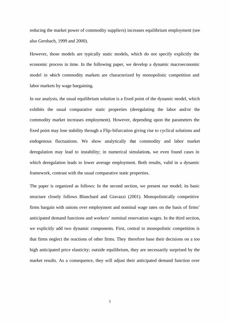
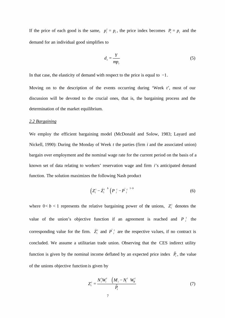
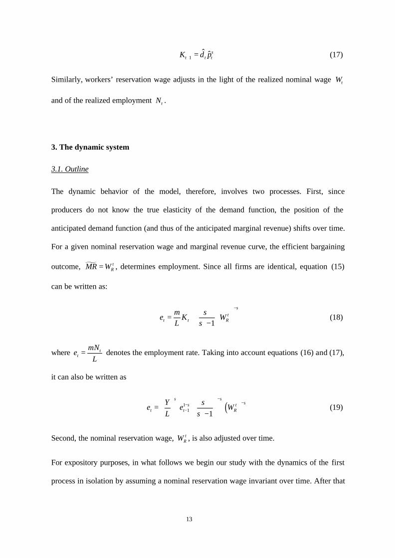
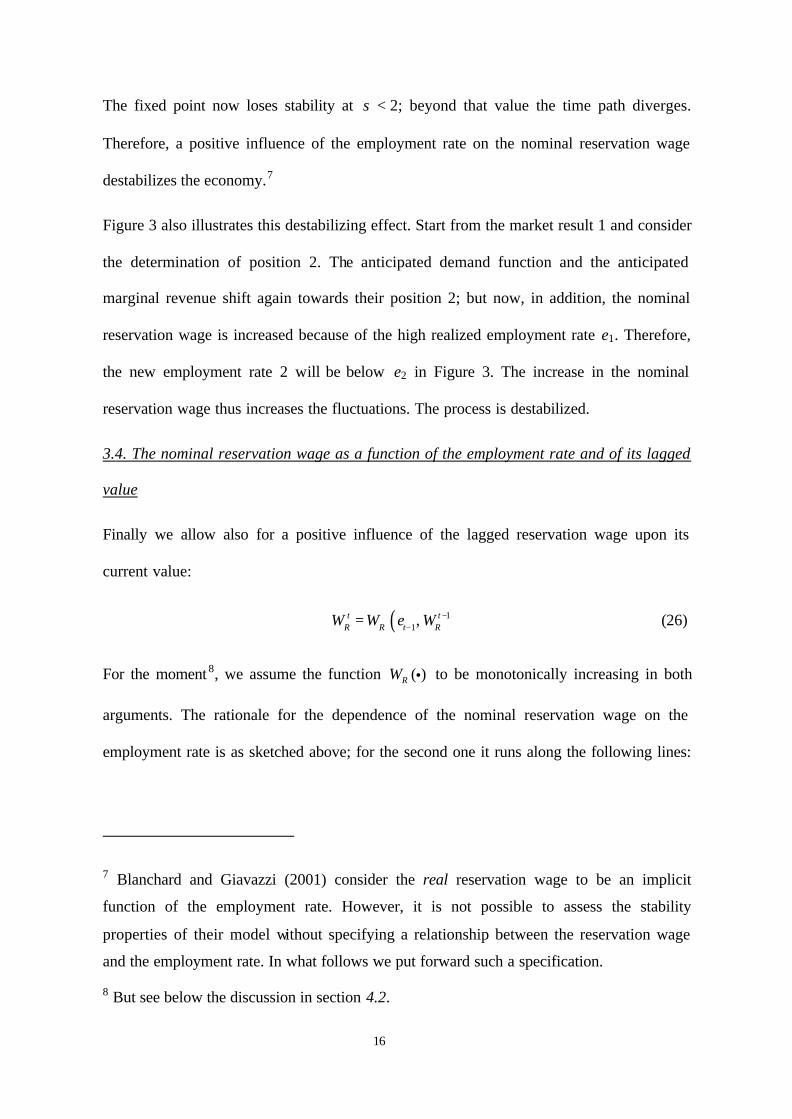
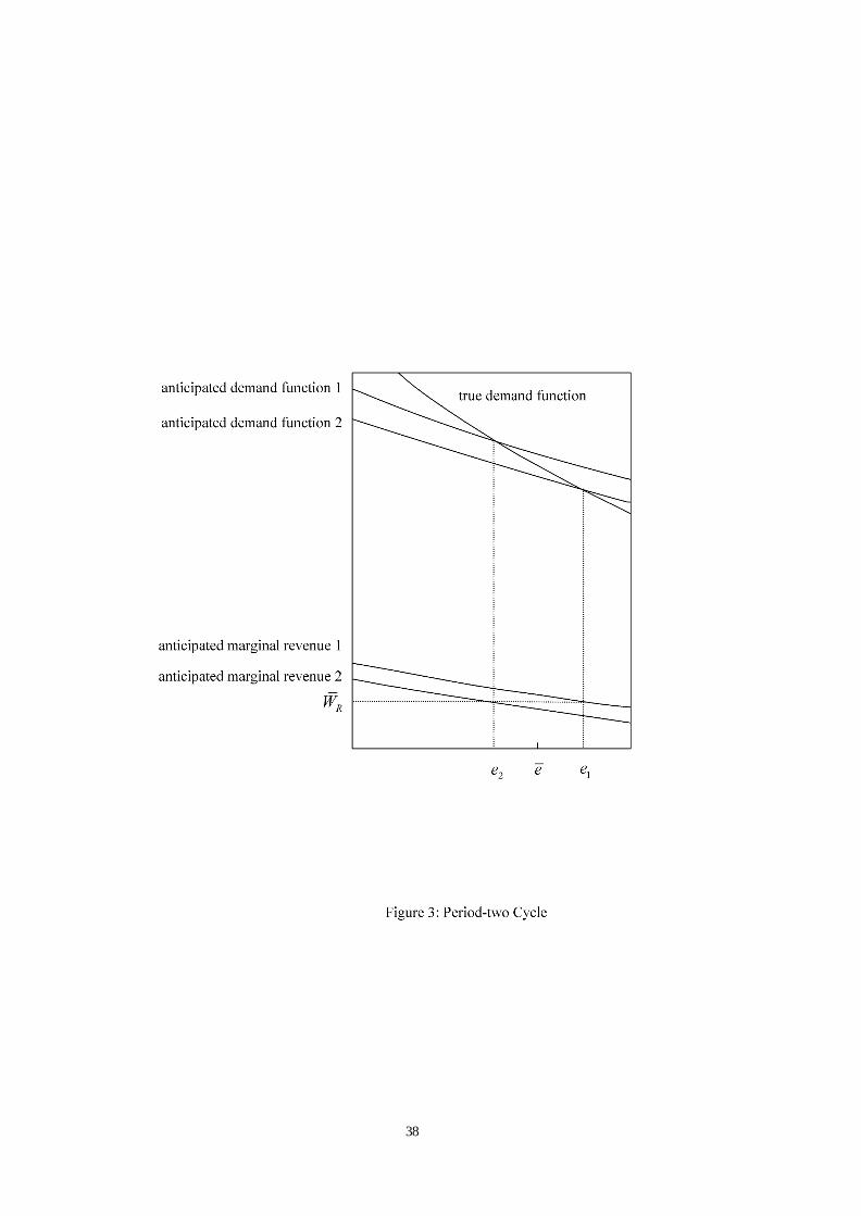
Figure 3 illustrates the period 2 cycle occurring precisely at σ = 2. The employment rate
alternates between e1 and e2; the anticipated demand and anticipated marginal revenue
functions shift accordingly. Starting with the anticipated demand function 1 and the
corresponding anticipated marginal revenue function 1 the bargaining process results in the
higher employment rate e1. The realized market price is below the anticipated one. The
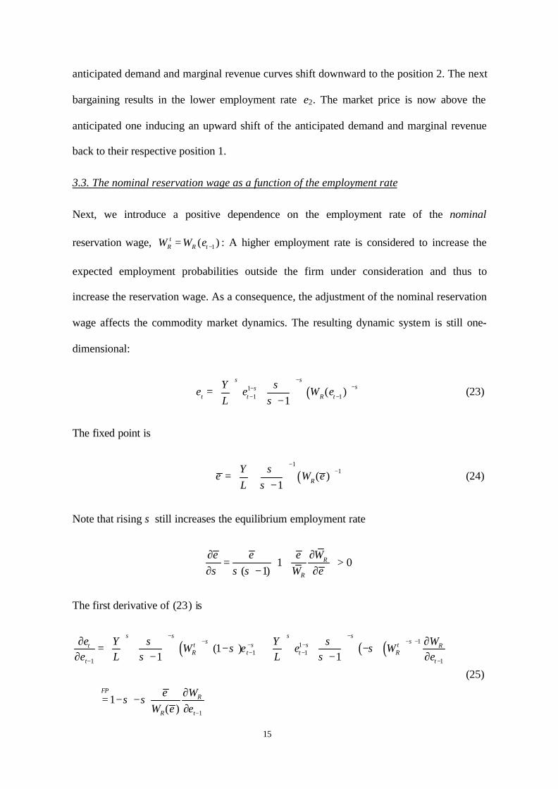
15
anticipated demand and marginal revenue curves shift downward to the position 2. The next
bargaining results in the lower employment rate e2. The market price is now above the
anticipated one inducing an upward shift of the anticipated demand and marginal revenue
back to their respective position 1.
3.3. The nominal reservation wage as a function of the employment rate
Next, we introduce a positive dependence on the employment rate of the nominal
reservation wage, 1( )−=tR R tW W e : A higher employment rate is considered to increase the
expected employment probabilities outside the firm under consideration and thus to
increase the reservation wage. As a consequence, the adjustment of the nominal reservation
wage affects the commodity market dynamics. The resulting dynamic system is still one-
dimensional:
( )11 1( )
1
σ σσσ σ
σ
−−−
− − = −
t t R t
Ye e W e
L (23)
The fixed point is
( )1
1( )1 R
Ye W e
Lσ
σ
−− = −
(24)
Note that rising σ still increases the equilibrium employment rate
1 0( 1)σ σ σ
∂∂= + > ∂ − ∂
R
R
We e eW e
The first derivative of (23) is
( ) ( ) ( ) 111 1
1 1
1
(1 )1 1
1( )
t tt RR t t R
t t
FPR
R t
e WY YW e e W
e L L e
WeW e e
σ σ σ σσ σσ σσ σ
σ σσ σ
σ σ
− −− − −− −
− −− −
−
∂ ∂ = − + − ∂ − − ∂
∂= − −
∂
(25)
16
The fixed point now loses stability at σ < 2; beyond that value the time path diverges.
Therefore, a positive influence of the employment rate on the nominal reservation wage
destabilizes the economy.7
Figure 3 also illustrates this destabilizing effect. Start from the market result 1 and consider
the determination of position 2. The anticipated demand function and the anticipated
marginal revenue shift again towards their position 2; but now, in addition, the nominal
reservation wage is increased because of the high realized employment rate e1. Therefore,
the new employment rate 2 will be below e2 in Figure 3. The increase in the nominal
reservation wage thus increases the fluctuations. The process is destabilized.
3.4. The nominal reservation wage as a function of the employment rate and of its lagged
value
Finally we allow also for a positive influence of the lagged reservation wage upon its
current value:
( )11,
−−=t t
R R t RW W e W (26)
For the moment 8, we assume the function ( )iRW to be monotonically increasing in both
arguments. The rationale for the dependence of the nominal reservation wage on the
employment rate is as sketched above; for the second one it runs along the following lines:
7 Blanchard and Giavazzi (2001) consider the real reservation wage to be an implicit
function of the employment rate. However, it is not possible to assess the stability
properties of their model without specifying a relationship between the reservation wage
and the employment rate. In what follows we put forward such a specification.
8 But see below the discussion in section 4.2.
17
a high reservation wage in t-1 will result in a high bargained nominal wage rate in t-1,
which in turn is expected to raise the nominal reservation wage in t.
The central dynamic system is now two-dimensional and given by equations (19) and (26).
In the fixed point the following holds
( )1
1
1 R
Ye W
Lσ
σ
−− = −
(27)
( ),R RW e Wθ= (28)
The Jacobian evaluated at the fixed point is given by
1
1
11
1t t
R Rt
R t R RE t t
R Rt
t R
e W e WW e W W
JW We W
σ σ σ −−
−−
∂ ∂− − − ∂ ∂ = ∂ ∂
∂ ∂
(29)
The trace and the determinant are
11
tr 1t t
R RE t
R t R
e W WJ
W e Wσ σ −
−
∂ ∂= − − +
∂ ∂ (30)
1det (1 )t
RE t
R
WJ
Wσ −
∂= −
∂ (31)
Figure 3 can be used to illustrate that the additional effect introduced by equation (26) is
potentially stabilizing. Start again with the market position realized in period 1 and consider
the determination of the position 2. The anticipated demand function and the anticipated
marginal revenue shift to their respective position 2. Two factors change the nominal
reservation wage. As in the previous case, the high employment rate e1 tends to increase it.
At the same time, the high employment rate e1 implies that the bargained nominal wage in

18
period 1 was comparatively low. This would reduce the nominal reservation wage, thus
introducing a stabilizing element.
Without specifying explicitly the dynamic adjustment process for the nominal reservation
wage, it is difficult to assess the stability properties. We provide such a specification in the
following section and explore the dynamics of the full model.
4. Fully specified dynamics and numerical simulations
4.1 . The dynamic adjustment process for the nominal reservation wage
The reservation wage in the bargaining process represents the income expected by the trade
union for members who do not find employment in the firm under consideration (see
Layard and Nickel, 1990). It therefore depends on the expected probability of finding
employment in other firms, on the wage rate expected to be paid by other firms and on the
unemployment benefit Bt.9 Consonant with the monopolistic competition set up, we assume
9 We did not incorporate explicitly the financing of the unemployment benefit. However,
we studied the case of financing it out of a general labor income tax that applies both to
workers and unemployed (similar to Calmfors and Johansson, 2001): Equ. (12) would be
modified to
( ) ( ) ( )( ) ( )1 11
tt t t t t t t t ii i i i t i R i i
t
NZ Z W W p W
P
ββ β βΠ Π τ
− − − − = − − −
) ) % % % .
where τ%t denotes the anticipated tax rate, with 1τ τ −=%t t , and where tiZ and t
iZ)
are now net
of taxation. On Tuesday, the tax rate is adjusted to match the benefit payments required by
the realized unemployment: ( ) ( )1 1t tt i i t t t t t t
i
W N W e L B e Lτ τ τ= = − −∑ and money holdings
are redistributed accordingly. The bargaining results and the following analysis are not
changed by this extension.
19
that the trade unions do not take into consideration reactions of other firms and the impact
of their own decisions on the aggregate variables. The expected probability of finding
employment in other firms and the expected wage rate outside the firm under consideration
is therefore given by the respective values realized in the previous period.
1 1 1(1 )tR t t t tW e W e B− − −= + − (32)
or using equation (13)
( )11 1
11
1t t
R t R t tW e W e Bσ β
σ−
− −+ − = + − −
(33)
For the unemployment benefit we consider two different specifications (see e.g. Layard et
al., 1991, and Pissarides, 1998) mirroring two possible institutional set-ups. The first is
close to a social assistance scheme according to which the compensation for the
unemployed is fixed in real terms (corresponding to a certain CES utility level ω ) and the
nominal payment is adjusted each period to the realized price, 1ˆt tB pω −= . In the second, the
compensation for the unemployed worker corresponds to a fraction of the nominal wage
rate she was receiving in the previous period, Bt = φWt–1, where 0 < φ < 1 is the replacement
ratio. The unemployment benefit systems in the OECD countries are found in between
those two extreme cases (see Goerke, 2000).
Such specifications will allow us to clarify the role of changes in parameters, which relate
to the unemployment benefit, as measures of (de)regulation in the labor market.
4.2 Unemployment benefit fixed in real terms
We consider first the institutiona l set up for the unemployment benefit close to a social
assistance system. The real unemployment benefit corresponds to a CES utility level of ω,
its nominal counterpart is given by 1ˆω −=t tB p . The dynamic system is
20
11 1
tt t R
Ye e W
L
σσσ σ
σ
−−−
= − (34)
( )11 1
1
11
1t t
R t R tt
YW e W e
Leσ β
ωσ
−− −
−
− + = + − − (35)
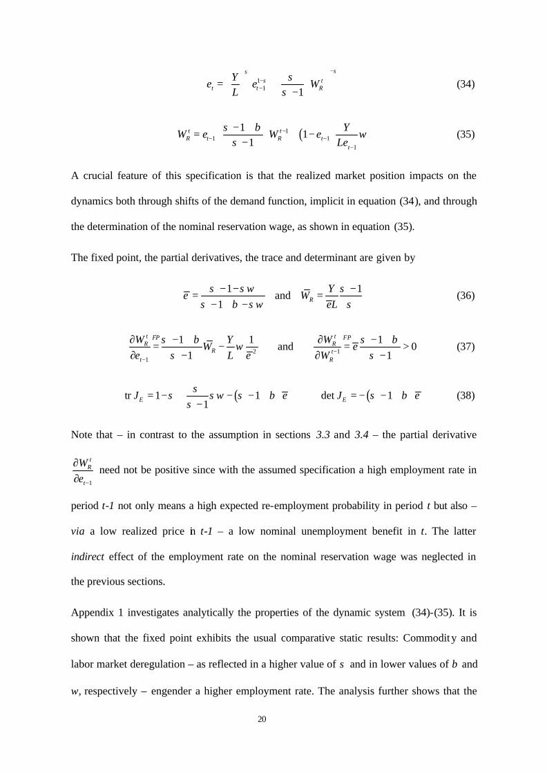
A crucial feature of this specification is that the realized market position impacts on the
dynamics both through shifts of the demand function, implicit in equation (34), and through
the determination of the nominal reservation wage, as shown in equation (35).
The fixed point, the partial derivatives, the trace and determinant are given by
1 1
and1 R
Ye W
eLσ σω σ
σ β σω σ− − −
= =− + −
(36)
2 11
1 1 1and 0
1 1
t tFP FPR R
R tt R
W Y WW e
e L e Wσ β σ β
ωσ σ−
−
∂ − + ∂ − += − = >
∂ − ∂ − (37)
( ) ( )tr 1 1 det 11E EJ e J e
σσ σω σ β σ β
σ= − + − − + = − − +
− (38)
Note that – in contrast to the assumption in sections 3.3 and 3.4 – the partial derivative
1−
∂∂
tR
t
We
need not be positive since with the assumed specification a high employment rate in
period t-1 not only means a high expected re-employment probability in period t but also –
via a low realized price in t-1 – a low nominal unemployment benefit in t. The latter
indirect effect of the employment rate on the nominal reservation wage was neglected in
the previous sections.
Appendix 1 investigates analytically the properties of the dynamic system (34)-(35). It is
shown that the fixed point exhibits the usual comparative static results: Commodity and
labor market deregulation – as reflected in a higher value of σ and in lower values of β and
ω, respectively – engender a higher employment rate. The analysis further shows that the
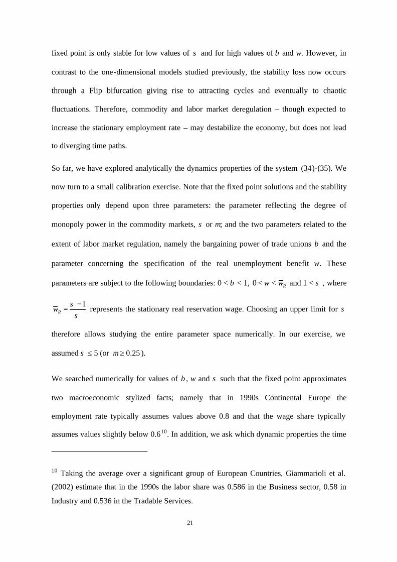
21
fixed point is only stable for low values of σ and for high values of β and ω. However, in
contrast to the one-dimensional models studied previously, the stability loss now occurs
through a Flip bifurcation giving rise to attracting cycles and eventually to chaotic
fluctuations. Therefore, commodity and labor market deregulation – though expected to
increase the stationary employment rate – may destabilize the economy, but does not lead
to diverging time paths.
So far, we have explored analytically the dynamics properties of the system (34)-(35). We
now turn to a small calibration exercise. Note that the fixed point solutions and the stability
properties only depend upon three parameters: the parameter reflecting the degree of
monopoly power in the commodity markets, σ or µ; and the two parameters related to the
extent of labor market regulation, namely the bargaining power of trade unions β and the
parameter concerning the specification of the real unemployment benefit ω. These
parameters are subject to the following boundaries: 0 < β < 1, 0 Rwω< < and 1 < σ , where
1Rw
σσ−
= represents the stationary real reservation wage. Choosing an upper limit for σ
therefore allows studying the entire parameter space numerically. In our exercise, we
assumed σ ≤ 5 (or 0.25µ ≥ ).
We searched numerically for values of β , ω and σ such that the fixed point approximates
two macroeconomic stylized facts; namely that in 1990s Continental Europe the
employment rate typically assumes values above 0.8 and that the wage share typically
assumes values slightly below 0.610. In addition, we ask which dynamic properties the time
10 Taking the average over a significant group of European Countries, Giammarioli et al.
(2002) estimate that in the 1990s the labor share was 0.586 in the Business sector, 0.58 in
Industry and 0.536 in the Tradable Services.
22
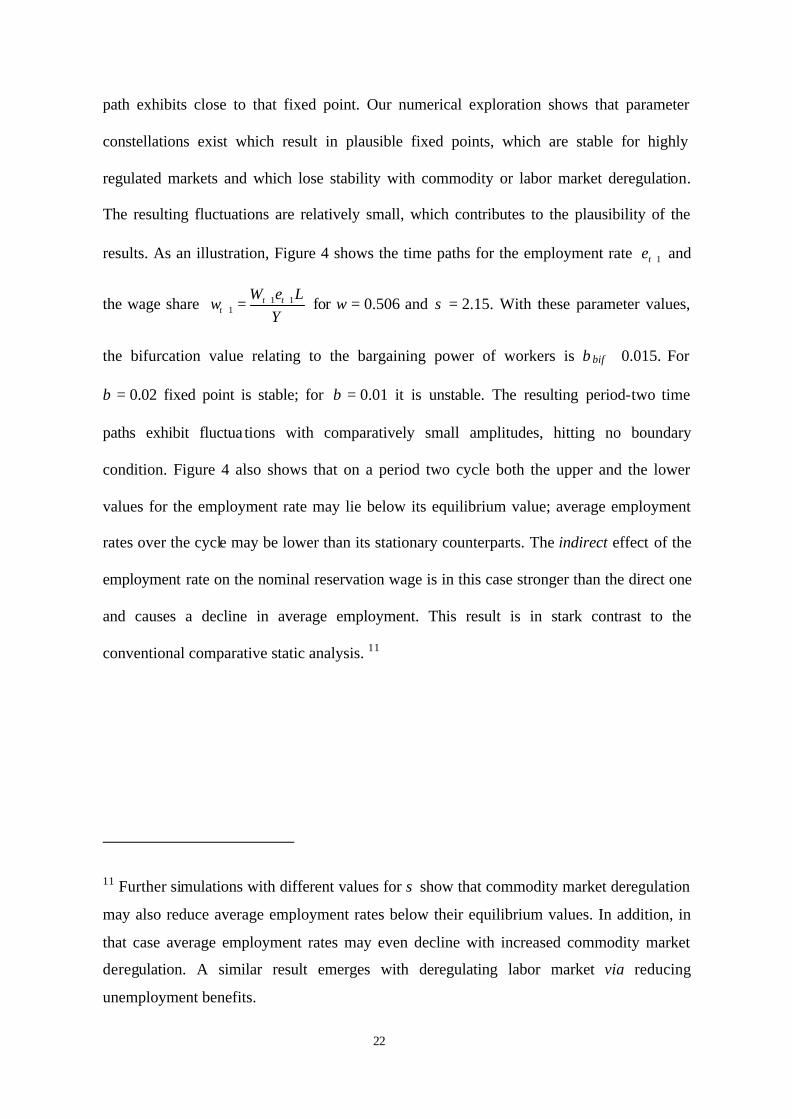
path exhibits close to that fixed point. Our numerical exploration shows that parameter
constellations exist which result in plausible fixed points, which are stable for highly
regulated markets and which lose stability with commodity or labor market deregulation.
The resulting fluctuations are relatively small, which contributes to the plausibility of the
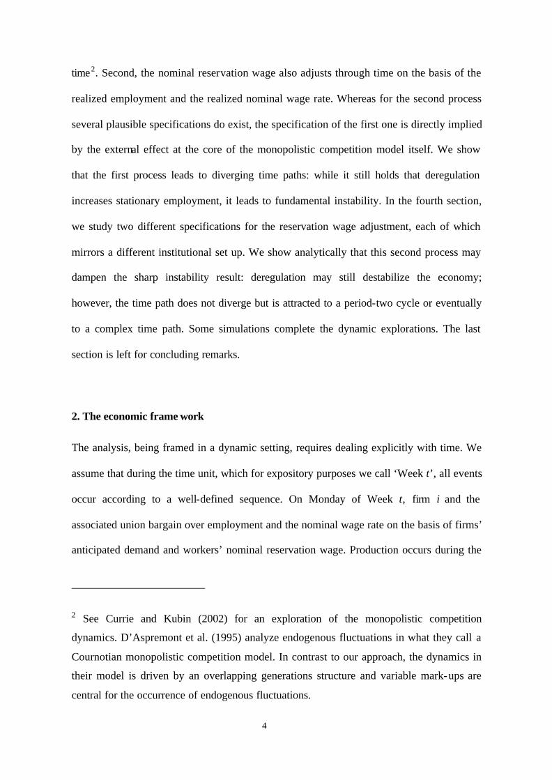
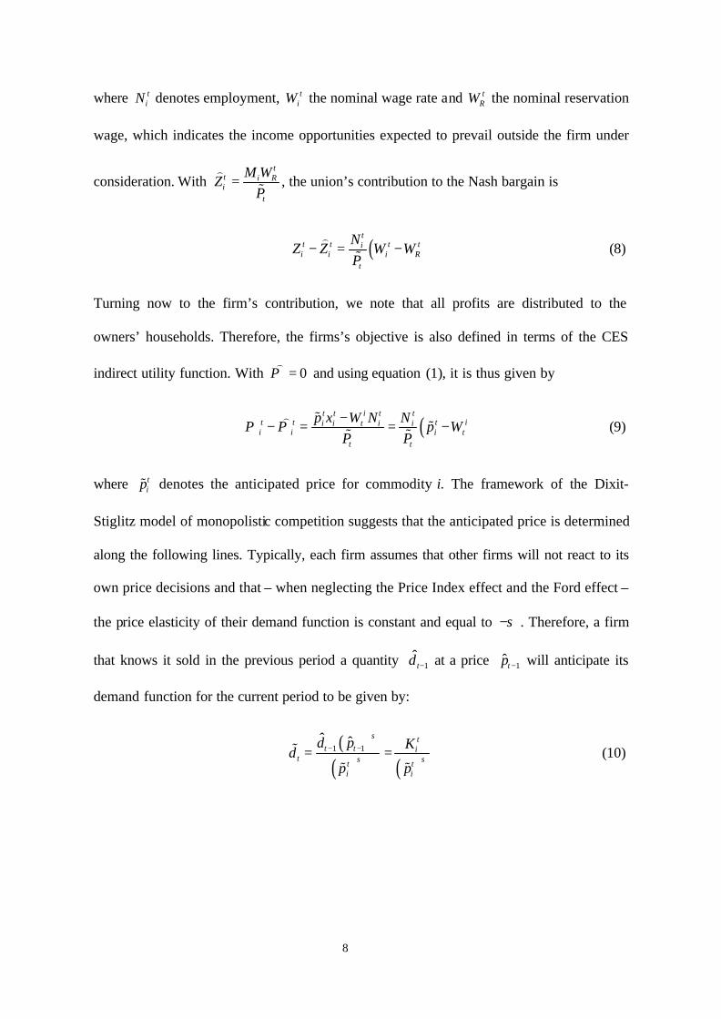
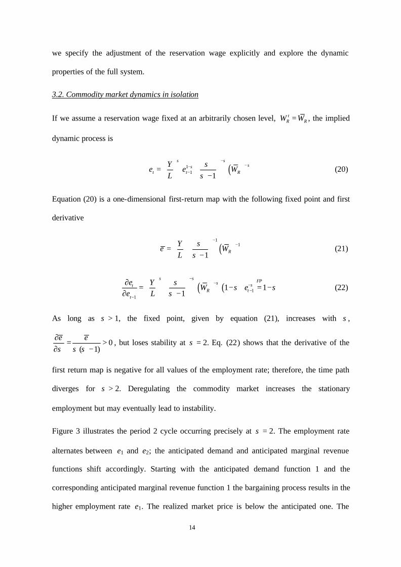
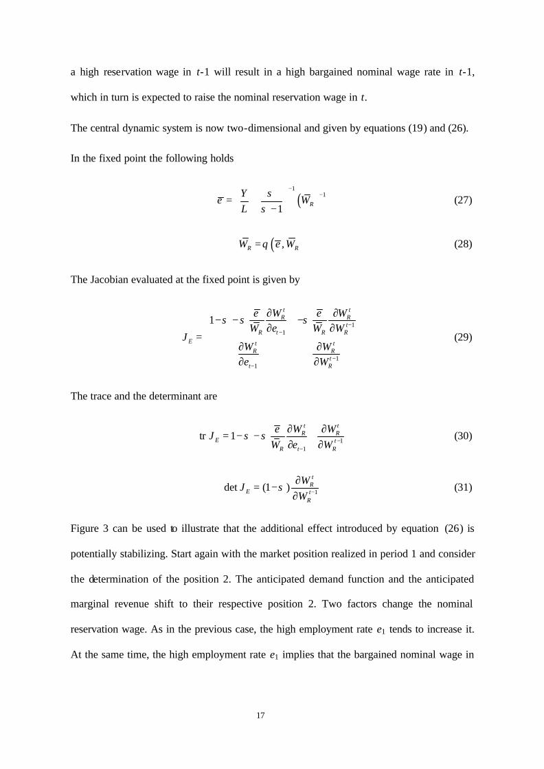
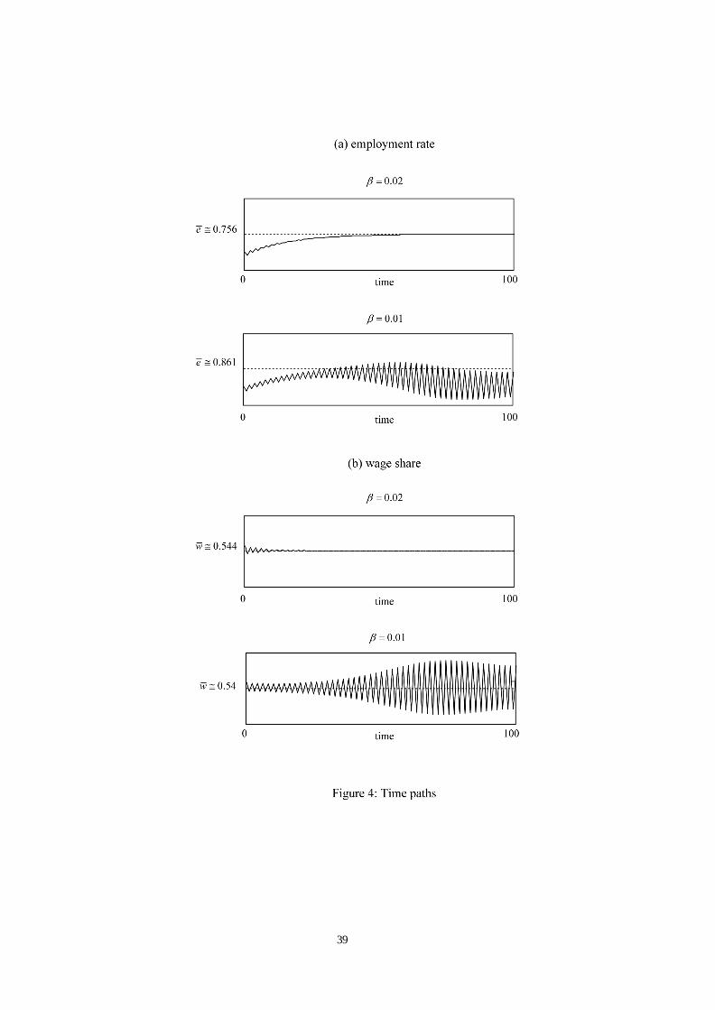
results. As an illustration, Figure 4 shows the time paths for the employment rate 1te + and
the wage share 1 11
t tt
W e Lw
Y+ +
+ = for ω = 0.506 and σ = 2.15. With these parameter values,
the bifurcation value relating to the bargaining power of workers is βbif ≅ 0.015. For
β = 0.02 fixed point is stable; for β = 0.01 it is unstable. The resulting period-two time
paths exhibit fluctua tions with comparatively small amplitudes, hitting no boundary
condition. Figure 4 also shows that on a period two cycle both the upper and the lower
values for the employment rate may lie below its equilibrium value; average employment
rates over the cycle may be lower than its stationary counterparts. The indirect effect of the
employment rate on the nominal reservation wage is in this case stronger than the direct one
and causes a decline in average employment. This result is in stark contrast to the
conventional comparative static analysis. 11
11 Further simulations with different values for σ show that commodity market deregulation
may also reduce average employment rates below their equilibrium values. In addition, in
that case average employment rates may even decline with increased commodity market
deregulation. A similar result emerges with deregulating labor market via reducing
unemployment benefits.
23
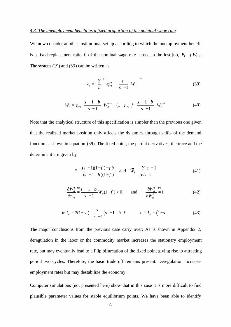
4.3. The unemployment benefit as a fixed proportion of the nominal wage rate
We now consider another institutional set up according to which the unemployment benefit
is a fixed replacement ratio φ of the nominal wage rate earned in the lost job, Bt = φWt–1.
The system (19) and (33) can be written as
11 1
tt t R
Ye e W
L
σσσ σ
σ
−−−
= − (39)
( )1 11 1
1 11
1 1t t t
R t R t RW e W e Wσ β σ β
φσ σ
− −− −
− + − + = + − − − (40)
Note that the analytical structure of this specification is simpler than the previous one given
that the realized market position only affects the dynamics through shifts of the demand
function as shown in equation (39). The fixed point, the partial derivatives, the trace and the
determinant are given by
( 1)(1 ) 1
and( 1 )(1 ) R
Ye W
eLσ φ φβ σσ β φ σ
− − − −= =
− + − (41)
11
1(1 ) 0 and 1
1
t tFP FPR R
R tt R
W WW
e Wσ β
φσ −
−
∂ − + ∂= − > =
∂ − ∂ (42)
( ) ( )tr 2(1 ) 1 det 11E EJ J
σσ σ β φ σ
σ= − + − + = −
− (43)
The major conclusions from the previous case carry over: As is shown in Appendix 2,
deregulation in the labor or the commodity market increases the stationary employment
rate, but may eventually lead to a Flip bifurcation of the fixed point giving rise to attracting
period two cycles. Therefore, the basic trade off remains present: Deregulation increases
employment rates but may destabilize the economy.
Computer simulations (not presented here) show that in this case it is more difficult to find
plausible parameter values for stable equilibrium points. We have been able to identify
24
stable two-cycles. The amplitude of the cyclical time path, however, is much higher than in
the previous case, and the employment rate hits quite often its upper boundary of one.12 In
the unstable region, further deregulation usually increases average employment rates even
above their corresponding equilibrium values.
5. Conclusion
In the previous paper, we have analyzed the dynamics of a model following closely the
prototype specification put forward by Blanchard and Giavazzi (2001) which combines
monopolistic competition in the commodity market and efficient bargaining in the labor
market. The dynamics results from two sources: First, inherent to monopolistic competition
is that each single supplier overestimates the price-elasticity of his demand function; each
single supplier is therefore necessarily surprised by the market outcome and will adapt his
anticipated demand function accordingly. Second, efficient bargaining processes are based
on a reservation wage indicating the expected income outside the firm under consideration.
This anticipation is also adjusted in the light of realized market results.
While the second process may be specified in various forms, the first one is directly implied
by the external effect at the core of the monopolistic competition model itself. It is difficult
to imagine fundamentally different specifications without leaving the assumed market
structure. We showed in the paper, that the first process destabilizes the economy:
Deregulation does increase the stationary employment rate, but engenders diverging time
paths. Introducing various plausible specifications for the adjustment process of the
12 We found in computer simulations the instability problem to be less severe with adaptive
expectations, which dampen the fluctuations of the anticipated demand function.
25
reservation wage dampens this sharp result: The stability loss occurs through a Flip
bifurcation giving rise not to diverging time paths but to attracting period-two cycles and
eventually to complex time paths. However, the basic trade-off remains: Deregulation
increases the stationary employment but may lead to instability with time paths exhibiting
in some cases even lower average employment rates.
References:
Bains, M. and A. Dierx, K. Pichlmann, W. Roeger, 2002, Structural reforms in labour and
product markets and macroeconomic performance in the EU, The EU Economy: 2002
Review, Chapter 2.
Benassy, J.-P., 1996, Taste for variety and optimum production patterns in monopolistic
competition, Economic Letters 52, 41-47.
Blanchard, O. and F. Giavazzi, 2001, Macroeconomic effects of regulation and
deregulation in goods and labor market, NBER-Working Paper 8120.
Blanchard, O. and N. Kiyotaki, 1987, Monopolistic Competition and the Effects of
Aggregate Demand, The American Economic Review 77, 647-666.
Blanchard, O., 2003, Macroeconomics (Prentice Hall).
Calmfors, L. and A. Johansson, 2001, Unemployment benefits contract length and nominal
wage flexibility, CESIfo Working Paper 514.
Currie, M. and I. Kubin, 2002, Complex Dynamics and Monopolistic Competition,
Beiträge zur Wirtschaftsforschung 02-01, Johannes Gutenberg-Universität Mainz,
Fachbereich Rechts- und Wirtschaftswissenschaften.
D’Aspremont, C. and R. Ferreira dos Santos, L. Gérard-Varet, 1990, On monopolistic
competition and involuntary unemployment, Quarterly Journal of Economics 105, 895-919.
D’Aspremont, C. and R. Ferreira dos Santos, L. Gérard-Varet, 1995, Market power,
coordination failures and endogenous fluctuations, in: H. Dixon and N. Rankin, The new
26
macroeconomics: imperfect markets and policy effectiveness (Cambridge University Press,
Cambridge) 94-138.
D’Aspremont, C. and R. Ferreira dos Santos, L. Gérard-Varet, 1996, On the Dixit-Stiglitz
Model of Monopolistic Competition, The American Economic Review 86, 623-629.
Dixit, A. and J. Stiglitz, 1977, Monopolistic Competition and Optimum Product Diversity,
The American Economic Review 67, 297-308.
Dixit, A. and J. Stiglitz, 1993, Monopolistic Competition and Optimum Product Diversity:
Reply, The American Economic Review 83, 302-304.
Gersbach, H., 1999, Product Market Competition, Unemployment and Income Disparities,
Weltwirtschaftliches Archiv 135, 221-240.
Gersbach, H., 2000, Promoting Product Market Competition to Reduce Unemployment in
Europe: An Alternative Approach?, Kyklos 53, 117-134.
Giammarioli, N. and J. Messina, T. Steinberger, C. Strozzi, 2002, European Labor Share
Dynamics: An Institutional Perspective, European University Institute, Working Paper Eco
2002-13.
Goerke, L., 2000, The Wedge, The Manchester School 68, 608-623.
Gordon, R., 1990, What is New-Keynesian Economics?, Journal of Economic Literature
28, 1115-1171.
Heijdra, B. and J. Ligthart, 1997, Keynesian Multipliers, Direct Crowding Out, and the
Optimal Provision of Public Goods, Journal of Macroeconomics 19, 803-826.
Heijdra, B. and J. Ligthart, F. van der Ploeg, 1998, Fiscal policy, distortionary taxation, and
direct crowding out under monopolistic competition, Oxford Economic Papers 50, 79-88.
Jerger, J., 2001, Globalization, Wage Setting and the Welfare State, Journal of Policy
Modelling 23.
Layard, R. and S. Nickell, 1990, Is unemployment lower if unions bargain over
employment?, The Quarterly Journal of Economics 105, 773-787.
Layard, R. and S. Nickell, R. Jackman, 1991, Unemployment (Oxford University Press,
Oxford).
27
Linnemann, L., 2001, The Price Index Effect, Entry, and Endogenous Markups in a
Macroeconomic Model of Monopolistic Competition, Journal of Macroeconomics 23, 441-
458.
McDonald, I. and R. Solow, 1983, Wage Bargaining and Employment, American
Economic Review LXXIII, 896-908.
McMorrow, K. and W. Roeger, 2000, Time - Varying Nairu / Nairu Estimates for the EU’s
Member States, ECFIN - Economic Papers 145.
Nickel, S., 1990, Unemployment: A Survey, The Economic Journal 100, 391-439.
Pissarides, C., 1998, The impact of employment tax cuts on unemployment and wages; The
role of unemployment benefits and tax structure, European Economic Review 42, 155-183.
Solow, R., 1999, Monopolistic Competition and Macroeconomic Theory (Cambridge
University Press, Cambridge).
Yang, X. and B. Heijdra, 1993, Monopolistic Competition and Optimum Product Diversity:
Comment, The American Economic Review 83, 295-301.
28
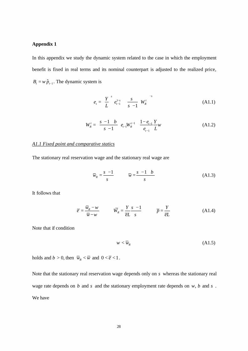
Appendix 1
In this appendix we study the dynamic system related to the case in which the employment
benefit is fixed in real terms and its nominal counterpart is adjusted to the realized price,
1ˆt tB pω −= . The dynamic system is
11 1
tt t R
Ye e W
L
σσσ σ
σ
−−−
= − (A1.1)
1 11
1
111
t t tR t R
t
e YW e W
e Lσ β
ωσ
− −−
−
−− + = + − (A1.2)
A1.1 Fixed point and comparative statics
The stationary real reservation wage and the stationary real wage are
1 1σ σ β
σ σ− − +
= =Rw w (A1.3)
It follows that
1R
R
w Y Ye W p
w eL eLω σ
ω σ− −
= = =−
(A1.4)
Note that if condition
Rwω < (A1.5)
holds and β > 0, then Rw w< and 0 1e< < .
Note that the stationary real reservation wage depends only on σ whereas the stationary real
wage rate depends on β and σ and the stationary employment rate depends on ω, β and σ .
We have

29
( )
( ) 2
1 ( )0
we
w w
ω β σ ωβσ σ σ ω
− + − ∂ = >∂ −
(A1.6)
( )
( )2 2 2
1 11 0 0
βσ σ
σ σ σ σ σ σσ
∂ ∂∂ ∂ − = − − = > = > ∂ ∂ ∂ ∂ R RW wY e w
eL e
(A1.7)
with ( 0) ( )( 1)
RW e efor
σ σ σ σ∂ ∂
≥ < ≤ >∂ ∂ −
The impact of changes in β is given by
2
0( )
ωβ σ ω
−∂= − <
∂ −Rwew
(A1.8)
2
1 10RW Y e w
Leσ
β σ β β σ∂ − ∂ ∂ = − = > ∂ ∂ ∂
(A1.9)
The impact of changes in ω is given by
2
10
( )e
wβ
ω σ ω∂
= − <∂ −
(A1.10)
2
10RW Y e
Leσ
ω σ ω∂ − ∂ = − > ∂ ∂
(A1.11)
A1.2 Bifurcation analysis
The Jacobian evaluated at the fixed point is
2
2
1 11
1 1
1 11 1
R RE
R
Y ee
LeW WJ
YW e
Le
σ β σ σ βσ σ ω
σ σ
σ β σ βω
σ σ
+ − + − − − − − − − = + − + − − − −
Determinant and Trace are:
( )det 1EJ eσ β= − + − (A1.12)
30
tr 1 ( 1)ω
σ β σ −
= − + − +
RE
R
wJ e
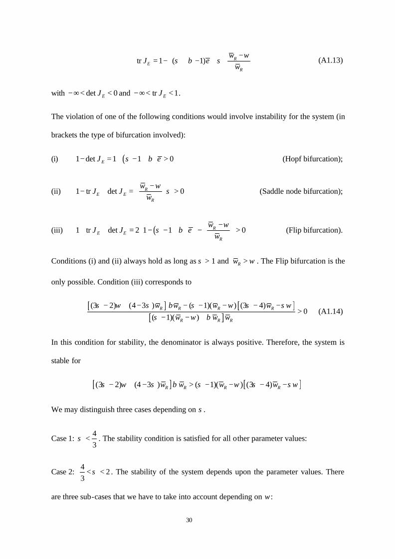
w (A1.13)
with det 0EJ−∞< < and tr 1EJ−∞< < .
The violation of one of the following conditions would involve instability for the system (in
brackets the type of bifurcation involved):
(i) ( )1 det 1 1 0EJ eσ β− = + − + > (Hopf bifurcation);
(ii) 1 tr det 0ω
σ −
− + = >
RE E
R
wJ J
w (Saddle node bifurcation);
(iii) ( )1 tr det 2 1 1 0ω
σ β −
+ + = − − + − >
RE E
R
wJ J e
w (Flip bifurcation).
Conditions (i) and (ii) always hold as long as σ > 1 and ω>Rw . The Flip bifurcation is the
only possible. Condition (iii) corresponds to
[ ] [ ]
[ ](3 2) (4 3 ) ( 1)( ) (3 4)
0( 1)( )
σ ω σ β σ ω σ σωσ ω β
− + − − − − − −>
− − +R R R R
R R R
w w w ww w w
(A1.14)
In this condition for stability, the denominator is always positive. Therefore, the system is
stable for
[ ] [ ](3 2) (4 3 ) ( 1)( ) (3 4)σ ω σ β σ ω σ σω− + − > − − − −R R R Rw w w w
We may distinguish three cases depending on σ.
Case 1: 43
σ < . The stability condition is satisfied for all other parameter values:
Case 2: 4
23
σ< < . The stability of the system depends upon the parameter values. There
are three sub-cases that we have to take into account depending on ω:

31
Case 2a: 3 43 2σ
ωσ
−<
− Rw . It follows ( ) ( )3 4 3 2 2σ σ ω σω− > − >Rw . In this case, the
stability condition is never satisfied.
Case 2b: 3 4 3 43 2σ σ
ωσ σ
− −< <
− R Rw w . The system is stable for
( 1)( )[(3 4) ]
0[(3 2) (4 3 ) ]
σ ω σ σωβ β
σ ω σ− − − −
> = >− + −
bif R R
R R
w ww w
(A1.15)
If β falls below this value, the system loses stability through a Flip bifurcation.
Case 2c: 3 4 3 43 2σ σ
ωσ σ
− −< < <
− R R Rw w w . The system is stable for
( 1)( )[(3 4) ]
0[(3 2) (4 3 ) ]
σ ω σ σωβ β
σ ω σ− − − −
> > =− + −
bif R R
R R
w ww w
That is, the system is always stable.
Case 3: 2 σ< . As for Case 2, the stability of the system depends upon the parameter
values. Depending on ω we may identify two sub-cases:
Case 3a: 3 43 2σ
ωσ
−<
− Rw . As in Case 2a, the stability cond ition is never satisfied.
Case 3b: 3 4 3 43 2σ σ
ωσ σ
− −< < <
− R R Rw w w . As in Case 2b, the system is stable for
( 1)( )[(3 4) ]
0[(3 2) (4 3 ) ]
σ ω σ σωβ β
σ ω σ− − − −
> = >− + −
bif R R
R R
w ww w
(A1.16)
If β falls below this value, the system loses stability through a Flip-bifurcation.

32
Appendix 2
In this appendix we examine some of the properties of the dynamic system related to the
case in which the employment benefit is a proportion of the nominal wage rate earned in
the lost job, Bt = φWt–1. The dynamic system is
11 1
tt t R
Ye e W
L
σσσ σ
σ
−−−
= − (A2.1)
[ ] 11
11 (1 )(1 )
1t t
R t RW e Wσ β
φσ
−−
− + = − − − − (A2.2)
A2.1 Fixed point and comparative statics
From (40) and (39), we solve for the stationary employment rate and reservation wage
( 1)(1 )( 1 )(1 )
eσ φ φβσ β φ
− − −=
− + − (A2.3)
1
R
YW
eLσ
σ−
= (A2.4)
Note that if condition
( 1)(1 ) 0σ φ φβ− − − > (A2.5)
holds and β > 0, then 0 1e< < .
The stationary price is Y
peL
= and the stationary nominal wage is 1
1 RW Wσ β
σ− +
=−
. It
follows that the stationary real wage and the stationary real reservation wage are identical
to the previous case:
1 1σ β σσ σ
− + −= =Rw w (A2.6)

33
From (A2.3), the stationary employment rate depends on φ, β and σ. The comparative
statics of the stationary state involves:
2
0( 1 ) (1 )
e βσ σ β φ
∂= >
∂ − + − (A2.7)
( )
( )2 2 2
1 1 11 0 0
βσ σ
σ σ σ σ σ σσ
∂ ∂∂ ∂ − = − − = > = > ∂ ∂ ∂ ∂ R RW wY e w
eLe
(A2.8)
with ( )0 ( )( 1)
RW e efor
σ σ σ σ∂ ∂
≥ < ≤ >∂ ∂ −
The impact of changes of β is given by
2
10
( 1 ) (1 )e σβ σ β φ
∂ −= − <
∂ − + − (A2.9)
2
1 10 0RW Y e w
Leσ
β σ β β σ∂ − ∂ ∂ = − > = > ∂ ∂ ∂
(A2.10)
The impact of changes of φ is given by
2
0( 1 )(1 )
e βφ σ β φ
∂= − <
∂ − + − (A2.11)
2
10RW Y e
Leσ
φ σ φ∂ − ∂ = − > ∂ ∂
(A2.12)
A2.2 Bifurcation analysis
The Jacobian evaluated at the fixed point is
( )
11 (1 )
11
1 11
RE
R
ee
WJ
W
σ βσ σ φ σ
σσ β
φσ
− + − − − − − = − +
− −

34
Determinant and Trace are:
det 1EJ σ= − (A2.13)
( )tr 2(1 ) 11EJ
σσ σ β φ
σ= − + − +
− (A2.14)
with det 0EJ−∞< < .
The violation of one of the following conditions would involve instability for the system (in
brackets the type of bifurcation involved):
(i) 1 det 0EJ σ− = > (Hopf bifurcation);
(ii) [ ]1 tr det ( 1)(1 ) 01E EJ J
σσ φ φβ
σ− + = − − − >
− (Saddle node bifurcation);
(iii) ( )1 tr det 1 3(1 ) 1 01E EJ J
σσ σ β φ
σ+ + = + − + − + >
− (Flip bifurcation).
Conditions (i) and (ii) always hold as long as condition (A2.5) holds. The Flip bifurcation is
the only possible. Condition (iii) corresponds to
[ ]2(3 ) 7 (1 ) 4 0φ σ β φ σ− − − − + < (A2.15)
If condition (A2.15) is not satisfied, the system loses stability through a Flip-bifurcation.
Define that value of σ corresponding to the highest root that satisfies condition (A2.15)
with an equality sign as
2 27 (1 ) 1 (1 ) 2(1 7 )
( , )2(3 )
zβ φ β φ β φ
φ βφ
− − + + − + +=
− (A2.16)
The system is stable for
3 4 1
1bif
σ σφ φ
σ β σ− − > ≡ − +
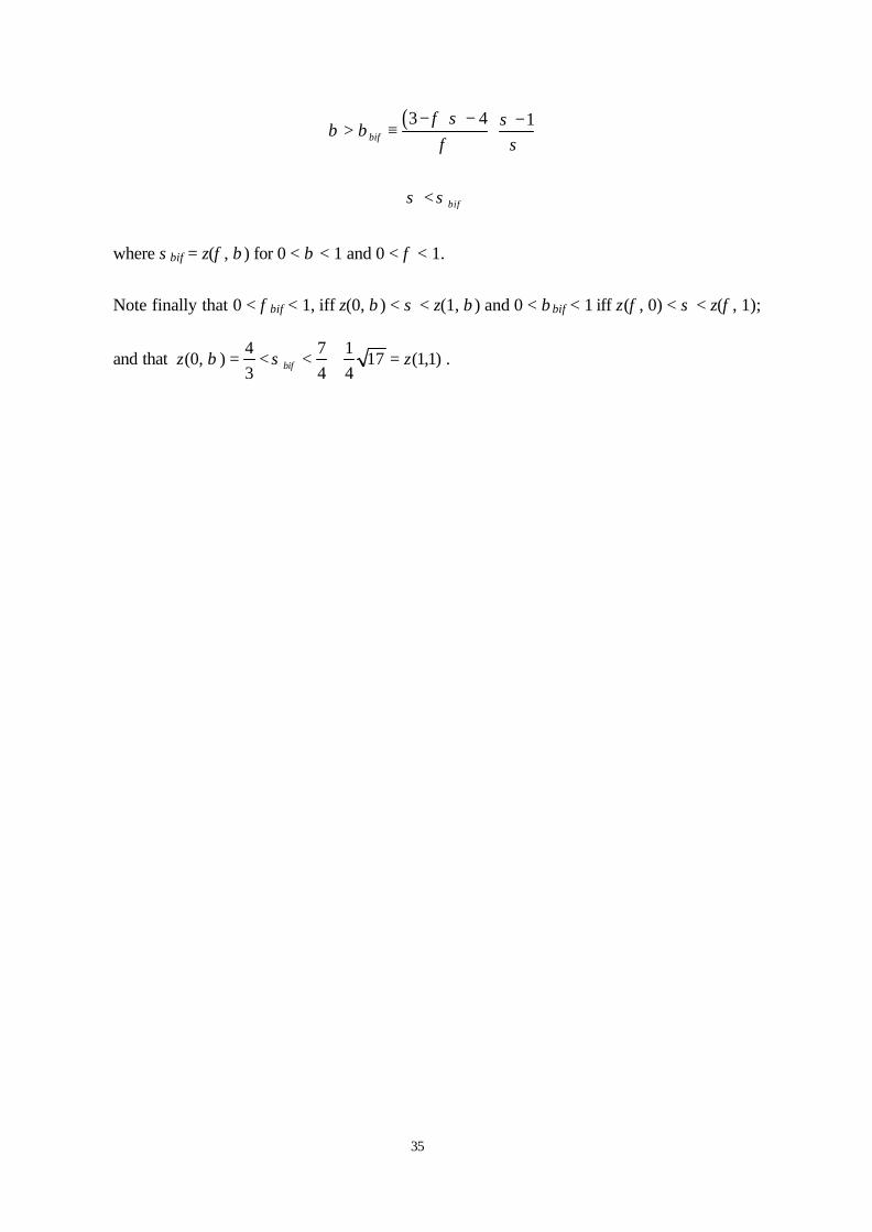
35
( )3 4 1
bif
φ σ σβ β
φ σ− − − > ≡
bifσ σ<
where σbif = z(φ, β) for 0 < β < 1 and 0 < φ < 1.
Note finally that 0 < φbif < 1, iff z(0, β) < σ < z(1, β) and 0 < βbif < 1 iff z(φ, 0) < σ < z(φ, 1);
and that 4 7 1
(0, ) 17 (1,1)3 4 4bifz zβ σ= < < + = .
36
37
38
39
Recommended