

iii

iv
DEDICATED TO
LATE FAJJI & LATE AMMI

v
ACKNOWLEDGMENT
All praise is to Allah (Subhanahu Wa Ta’aala) with whose mercy and blessings I have
achieved what I have achieved today. Peace and blessings of Allah be upon the final
prophet.
I take this opportunity to thank my advisor Dr. Hussain Nasir Al-Duwaish. for his
guidance and motivation which he has extended to me throughout my thesis and during
my stay at this university. I am grateful to him for his unlimited favors and help which he
extended to me during my rough time in my life and for his help in the administrative
affairs of mine related to the university. I extend my gratitude to my Co-Advisor, Dr.
Muhammad A. Al-Arfaj, for his help and guidance in making my dream come true. I am
grateful to him for his time which he has given to me without bounds for the completion
of my thesis and for his faith and trust which he had in me during my work with him.
I gratefully acknowledge Dr. Al-Baiyat Samir A. for his advice and guidance through my
research and Dr. Bakhashwain Jamil M. for his profound support and Dr Mantawy
Abdel-Aal H. for his help in my work.
I further extend my thanks to Moshood who has been more than a help ever since I
started my work in this area and has always been there to help me anytime I need him. I

vi
thank my department and especially my chairman for providing me with abundant
facilities of PC-Labs for simulation and helping me in my issues.
It would be ungrateful if I forget my family at this time, I am grateful to my father,
mother and my sisters for their constant prayers their patience and faith in me, a pillar of
support ever since I was born. I also extend my thanks to Liaqat bhaiya, Mahamid
Bhaiya, Ismail Bhai, Ashraf Bhaiya.
Last but not the least my armada of friends who always kept me on the edge of my seat
and provided me with every thing I needed to realize this dream. To mention a few:
AmerBhai, Faisal, Ayub, Abbas, Baber, Riyaz, Abdul Hameed, FasiBhai, AneesBhai,
Abdul Hafeez(Shaukat), Baba, Aleem, Ilyas, Wajid, Mansoor, Kareem, Rahman, Asif,
Asim, Kazim, Rahim, Tanveer, Mubashir, Guddu, Aslam, Faizan, Allauddin. And seniors
SohelBhai, RazaBhai, BasharBhai, TayyabBhai and Nasir Bhai(AmeerSaab).
Special thanks to Sheikh Saleh Al-Munajjid, Moulana Abdul Quavi Sahab, Dr. Hafiz
Afzal Sahab, Dr. Zafarullah Khan Sahab, Dr. Abdul Aziz Sahab and My masters who
taught me to read Holy Qur’aan.
Thank you one and all.
vii
TABLE OF CONTENT
ACKNOWLEDGMENT ..............................................................................................v
TABLE OF CONTENT................................................................................................vii
LIST OF TABLES ........................................................................................................x
LIST OF FIGURES ......................................................................................................xi
THESIS ABSTRACT ...................................................................................................xii
THESIS ABSTRACT (ARABIC)................................................................................xiii
CHAPTER 1..................................................................................................................1
INTRODUCTION.........................................................................................................1
1.1 Introduction and Motivation..............................................................................1
1.2 Literature Review................................................................................................3 1.2.1 Particle Swarm Optimization ........................................................................3 1.2.2 Reactive Distillation Column ........................................................................6
1.3 Objectives .............................................................................................................8
1.4 Research Methodology........................................................................................10
1.5 Significance ..........................................................................................................12
1.6 Contribution.........................................................................................................13
CHAPTER 2..................................................................................................................14
PARTICAL SWAM OPTMIZATION .......................................................................14
2.1 The Basic Particle Swarm...................................................................................14
2.1.1 The Algorithm ...............................................................................................17
2.2 Extensions to the Particle Swarm ......................................................................21 2.2.1 Controlling the Convergence.........................................................................21 2.2.2 Avoiding Premature Convergence ................................................................23
viii
2.2.3 Speeding up Convergence .............................................................................24
2.3 Parameter Selection.............................................................................................25
2.3.1 The Control Parameters 1φ and 2φ ................................................................27 2.3.2 The Inertia Weight ω ....................................................................................29 2.3.3 The Constriction Factor χ ............................................................................30 2.3.4 The Maximum Velocity vmax .........................................................................32 2.3.5 The Neighborhood Topology ........................................................................33
2.4 Constrained Problems.........................................................................................34
CHAPTER 3..................................................................................................................37
HYBRID INTERGER PSO .........................................................................................37
3.1 Background..........................................................................................................37 3.1.1 Hybrid PSO ...................................................................................................37 3.1.2 Integer PSO ...................................................................................................43
3.2 Hybrid-Integer PSO ............................................................................................48
3.3 Test Functions......................................................................................................52
CHAPTER 4..................................................................................................................56
OPTIMIZATION PROBLEM FORMULATION.....................................................56
4.1 Reactive Distillation Column..............................................................................57 4.1.1 Process Modeling ..........................................................................................61 4.1.2 State space Model..........................................................................................66 4.1.3 Optimum Steady State Design ......................................................................68
4.2 Cost Function Formulation ................................................................................70
CHAPTER 5..................................................................................................................74
SIMULATION AND SETUP.......................................................................................74
5.1 PC Setup...............................................................................................................74
5.2 Optimization Setup..............................................................................................75 5.2.1 HI-PSO ..........................................................................................................75
ix
5.2.2 Reactive Distillation Column ........................................................................76 5.2.2.1 Initial Values...........................................................................................76 5.2.2.2 Range of Variables..................................................................................78 5.2.2.3 Process Run Time ...................................................................................79
5.3 Objective Function ..............................................................................................83
5.4 Algorithm .............................................................................................................84
5.5 Results and Discussions.......................................................................................86 5.5.1 Optimization of Trays ...................................................................................86 5.5.2 Optimization of Trays and Column Pressure ................................................91 5.5.3 Optimization of Trays, Column Pressure and Feed Locations......................96
CHAPTER 6..................................................................................................................103
CONCLUSIONS AND RECOMMENDATIONS......................................................103
6.1 Conclusions ..........................................................................................................103
6.2 Recommendations for Future Work..................................................................104
REFERENCES..............................................................................................................106
VITAE .......................................................................................................................111
x
LIST OF TABLES
Table 3.1 Laskari et al. PSO parameters.........................................................................53
Table 3.2 Performance of Hybrid Integer PSO...............................................................54
Table 4.1. Physical Properties.........................................................................................69
Table 4.2. Optimum Design for single-column process .................................................70
Table 5.1 Brute force Tray Optimization........................................................................90
Table 5.2 Bruteforce - Tray and Pressure Optimization .................................................93
Table 5.3 Tray + Pressure + Feed Worst Cases..............................................................101
Table 5.4 Tray + Pressure + Feed Best Cases.................................................................102
xi
LIST OF FIGURES
Figure 1.1 Research Methodology..................................................................................11
Figure 2.1: a) fully connected b) k-best with k = 2, and c) twheel topology ..................34
Figure 3.1 Basic PSO vs Hybrid PSO for Rastrigins Function.......................................42
Figure 3.2 Integer PSO Example ....................................................................................47
Figure : 3.3 Comparison of PSO with Hybrid PSO........................................................49
Figure : 3.4 Algorithm of Hybrid Integer PSO...............................................................51
Figure 3.5 Hybrid Integer PSO vs basic PSO and Integer PSO......................................52
Figure 4.1 Reactive Distillation Column ........................................................................59
Figure 5.1 Selected Composition Profile for 6th -8th Hr of RDC operation...................81
Figure 5.2 Selected Composition Profile for 14th to 16th Hr of RDC Operation ............81
Figure 5.3 Selected Composition Profile for 30th -32nd Hr of RDC operation ...............82
Figure 5.4: Hybrid Integer - PSO Algorithm..................................................................85
Figure 5.5 Composition Profile [7 6 7] Base Case .........................................................86
Figure 5.6 Optimization of Vs, Objective 1-Trays .........................................................87
Figure 5.7 Composition Bottom and Distillate, Objective 1-Trays ................................89
Figure 5.8 Composition Profile [13 8 12] Objective 1-Trays Optimization...................90
Figure 5.9 Optimization of Vs Objective 2–Trays and Column Pressure ......................92
Figure 5.10 Products Purity Percentage Composition Objective 2–Trays and Column
Pressure Optimization...................................................................................95
Figure 5.11 Composition Profile Objective 2 - Trays and Column Pressure Optimization
.......................................................................................................................96
Figure 5.12 Optimization of Vs Objective 3 – Trays, Column Pressure and Feed
Locations.......................................................................................................97
Figure 5.13 Products Purity Percentage Composition Objective 3 - Trays, Column
Pressure and Feed Locations.........................................................................99
Figure 5.14 Composition Profile Objective 3 - Trays, Column Pressure and Feed
Locations.......................................................................................................100
xii
THESIS ABSTRACT
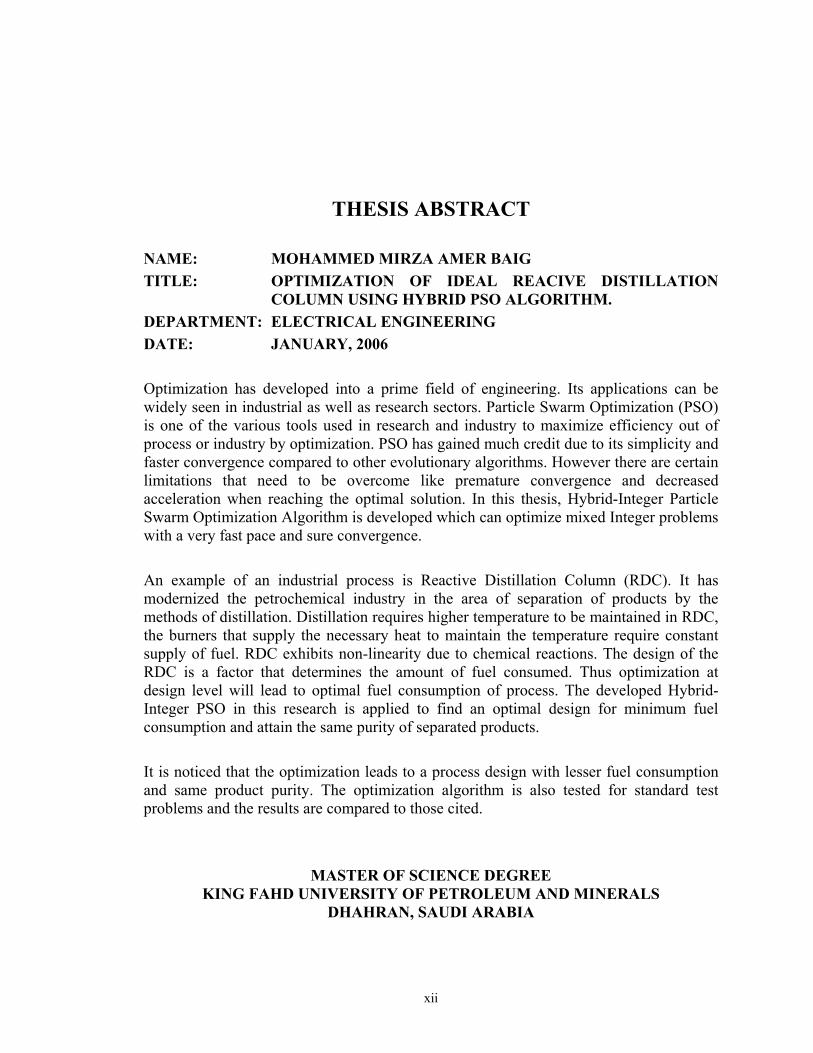
NAME: MOHAMMED MIRZA AMER BAIG TITLE: OPTIMIZATION OF IDEAL REACIVE DISTILLATION
COLUMN USING HYBRID PSO ALGORITHM. DEPARTMENT: ELECTRICAL ENGINEERING DATE: JANUARY, 2006 Optimization has developed into a prime field of engineering. Its applications can be widely seen in industrial as well as research sectors. Particle Swarm Optimization (PSO) is one of the various tools used in research and industry to maximize efficiency out of process or industry by optimization. PSO has gained much credit due to its simplicity and faster convergence compared to other evolutionary algorithms. However there are certain limitations that need to be overcome like premature convergence and decreased acceleration when reaching the optimal solution. In this thesis, Hybrid-Integer Particle Swarm Optimization Algorithm is developed which can optimize mixed Integer problems with a very fast pace and sure convergence. An example of an industrial process is Reactive Distillation Column (RDC). It has modernized the petrochemical industry in the area of separation of products by the methods of distillation. Distillation requires higher temperature to be maintained in RDC, the burners that supply the necessary heat to maintain the temperature require constant supply of fuel. RDC exhibits non-linearity due to chemical reactions. The design of the RDC is a factor that determines the amount of fuel consumed. Thus optimization at design level will lead to optimal fuel consumption of process. The developed Hybrid-Integer PSO in this research is applied to find an optimal design for minimum fuel consumption and attain the same purity of separated products. It is noticed that the optimization leads to a process design with lesser fuel consumption and same product purity. The optimization algorithm is also tested for standard test problems and the results are compared to those cited.
MASTER OF SCIENCE DEGREE
KING FAHD UNIVERSITY OF PETROLEUM AND MINERALS DHAHRAN, SAUDI ARABIA
xiii
THESIS ABSTRACT (ARABIC)
ملخص الرسالة
محمد ميرزا أمير باج: االسم Hybrid PSO Algorithmsالتصميم األمثل لعملية صناعية باستخدام : عنوان الرسالة
الهندسة الكهربية: التخصص 2006يناير : تاريخ التخرج
الصناعة والنطاق أصبح الوصول للتصميم األمثل أحد المجاالت الرئيسية في الهندسة التي لها تطبيقات واسعة في
أحد األدوات المستخدمة في المجال الصناعي والبحثي للحصول على اآبر آفاءة ممكنة لعملية أو صناعة ما . البحثياآتسبت هذه الطريقة أهمية آبيرة بسبب بساطتها وسرعة . Particle Swam Optimization (PSO)هو
في هذه الرسالة تم . ه الطريقة بعض القيود التي يجب أن تعالجالوصول للنتائج مقارنة بالطرق القديمة لكن توجد لهذ لمعالجة المشاآل الصحيحة Hybrid-Integer Particle Swarm Optimization Algorithmتطوير
. المختلطة بخطوة سريعة جدا وتقارب أآيدReactive Distillation Column (RDC) تي طورت الصناعات هو أحد األمثلة على العمليات الصناعية ال
يتطلب التقطير توفير درجة حرارة عالية والتي بدورها . البتروآيماوية في مجال فصل المنتجات بطريقة التقطيرتتميز بأنها معقدة وغير خطية بدرجة آبيرة وباعتماد آمية الوقود (RDC)عملية ال. تتطلب آمية وقود مناسبةفي . مثل في مرحلة التصميم بالتالي يؤدي إلى االستهالك المثالي للوقودالوصول للحل األ. المستهلكة على التصميم
للوصول للتصميم األمثل الستهالك أقل آمية من الوقود Hybrid-Inteeger PSOهذا البحث تم استخدام طريقة ال ول للتصميم األمثل تم اختبار هذه الطريقة أيضا في الوص. والحفاظ على نفس درجة نقاوة المنتجات التي يتم فصلها
. لبعض المشاآل القياسية والنتائج آانت مقاربة للنتائج المنشورة
ردرجة ماجستي جامعة الملك فهد البترول و المعدن
31261 -الظهران المملكة العربية السعودية
1
CHAPTER 1
INTRODUCTION
1.1 Introduction and Motivation
Optimization is one of the major quantitative tools in the machinery of decision-making.
A wide variety of problems in the design, construction, operation and analysis of
industrial process can be resolved by optimization [ 1]. A typical engineering problem can
be posed as follows: given a process that can be represented by mathematical equations
and a performance criterion such as minimizing annual cost of maintenance. The goal of
optimization is to find the values of the variables in the process that yield the best value
of the performance criterion. Together the process and the performance criterion
represent the optimization problem [ 1]. One such tool of optimization which has gained
high recognition recently is Particle Swarm Optimization which is generally referred to as
PSO.
The industrial sector has always sought after reducing the capital investment and
maximizing the profits based on the investments. An important and ever growing sector
in the industry is the “Reactive Distillation” in the chemical industry. Reactive
Distillation is used to separate chemical reactants after the reaction into different
2
products. Its importance and benefits are being realized everywhere in the world due to
its single column reaction and separation ability. This compact nature of Reactive
Distillation has led to its important role and has obliged the industry to switch from
classical methods of separate reaction and distillation to a compact one “Reactive
Distillation Column” where both the process of reaction and separation take place [2]. A
commending effort has been done by Al-Arfaj and Luyben in designing an ideal
hypothetical reactive distillation column. Where all the complexities are stripped aside
and component control of the process is given importance [20]. One of the major
requirements of the “Reactive Distillation Column” is that it requires a constant supply of
heat so as to maintain the temperature of reaction in the entire section. This requires a
heat source which generally is a burner and is called reboiler.
Little has been done in the research area to develop a model which can provide an
optimal design which consumes least amount of fuel required by the burner. With the rise
in the cost of oil and its ever increasing demand, it is of great significance to have a
model that consumes least amount of fuel but delivers the exact concentration of
products.
This research is a step towards the development of optimal reactive distillation column so
as to reduce the capital incurred on the fuel consumption. A floating model is step wise
developed out of an existing model [20] thereafter a hybridized version of PSO is applied
3
to find the optimal design parameters like Trays, Pressure and the Feed locations in the
reactive distillation column so as to produce the same products concentration with
minimal of fuel consumption.
1.2 Literature Review
1.2.1 Particle Swarm Optimization
Particle Swarm Optimization (PSO) is a stochastic optimization algorithm that belongs to
the category of swarm intelligence methods [11]. PSO has attained increasing popularity
due to its ability to solve efficiently and effectively a plethora of problems in diverse
scientific fields [21]. Most of these problems involve the minimization of a static
objective function, i.e., the main goal is the computation of a global minimizer that does
not change.
The research has grown extensively in the field of optimization and particularly in the
field of PSO due to its ever increasing popularity. All this started when the concept of
function-optimization by means of a particle swarm was introduced by James Kennedy,
Russel and Eberhart [12]. Later they developed the algorithm and laid principles to what
is today called as Swarm Intelligence [11], In which they defined the five basic principles
on which the Swarm Intelligence was introduced.
4
Angeline [13] and Kennedy [14] discussed the drawback of simple PSO as was
formulated first in comparison with the Evolutionary Algorithms. And it was not until the
Vmax operator was introduced by Kennedy [11] that made PSO worth to be recognized as
a competitor to the evolutionary algorithms and Angeline [13] verified this with his
comparisons. Later versions of Eberhart and Shi [18] introduced the concept of inertia
weights where the velocities are multiplied by the inertia factor before updating and
Maurice introduced constriction factor [15] which constricts the velocity to their present
velocity by multiplying with the constriction factor before updating.
PSO converges very rapidly for uni-modal problems, but for multi-modal problems there
is a great risk of the algorithm getting struck in the local optima, i.e. premature
convergence, in order to avoid this one would have to look into all possible local optima
before deciding on the global optimal value. This by itself is cumbersome the algorithm
will take a large amount of time to cruise through all the local solutions before
converging on the global optima. One such method to avoid this premature convergence
was addressed by Lovberg [16] wherein they renewed the swarm by breeding some of the
particles and called this algorithm the Hybrid-PSO a merger of Evolutionary algorithms
with the basic PSO.
In order to improve the convergence speed of the PSO for multi-modal problems,
Kennedy [11] proposed that if the an approximate clusters of particles which are assumed
5
to be near the global optima should replace the present global and local trajectories so
that they can converge faster to the global optima.
Kennedy in [14] came up with the idea of neighborhood where in information between
the particles could be shared so as to enhance the search space and achieve better
convergence, e.g. In here the particles share the information with the two adjacent
particles. He further discussed types of neighborhood techniques in his work which can
influence the convergence.
The important criteria once the PSO algorithm is ready is to have a proper tuning of the
parameters so that the global optimal solution can be achieved very fast and with out
getting into the premature convergence pit. Several papers have mentioned the parameter
selection criteria prominent among them are Shi and Eberhart[18][19] , Carlisle and
Dozier [17], Clerc and Kennedy [15]and Angeline [13] a few out of vast researchers.
A wide variety of problems can be represented as discrete optimization models. Integer
programming has many applications one among them is the training of neural networks
with integer weights, where the activation function and weight values are confined in a
narrow band of integers. Laskari et al. [36] developed Particle Swarm Optimization to
handle integer problems and have compared their work with the classical Branch and
Bound technique and concluded that PSO out performs Branch and Bound.
6
1.2.2 Reactive Distillation Column
Reactive distillation is the coupling of both physical separation and chemical reaction in
one unit operation. It has been employed in industry for many decades, and its area of
application has grown significantly. A reactive distillation column is usually split into
three sections: reactive section, stripping section and rectifying section. In the reactive
section, the reactants are converted into products, and where, by means of distillation, the
products are separated out of reactive zone. The tasks of the rectifying and stripping
sections depend on the boiling points of the reactant and product.
Several researchers have worked extensively on the conceptual design and process
optimization of reactive distillation [1, 2]. Al-Arfaj and Luyben [3] have discussed the
Effect of number of trays of fractionation on the performance of Reactive Distillation
column and concluded that increasing or decreasing the fractionation trays does not
degrade the performance maintaining the same concentration of the products.
Al-Arfaj and Luyben [20] studied the control of reactive distillation column that
produced two products from a single reactive column by feeding exactly stoichiometric
amount of the two fresh feed streams. They explored control structures, all of which
included the measurement of composition of one of the reactants inside the reactive
7
section of the column. This composition is then used to adjust the appropriate fresh feed
stream.
Olanrewaju [41] in his thesis developed linear online estimators to facilitate the
measurement of samples under erroneous conditions and later developed estimator based
control on reactive distillation column.
However, only a few papers have appeared that discuss the closed-loop optimization of
reactive distillation column. Sane et al. [38] have shown that the introduction of a
different tray holdup in the stripper and rectifier section of a continuous kinetically
controlled reactive distillation column facilitates the design procedure. Their design
allows minimizing investment related costs such as the column height and the amount of
catalyst.
Cardoso et al. proposed an optimization model for the MINLP(Mixed integer Non-linear
Programming) formulation of the reactive distillation columns using simulated annealing
which gives optimal number of trays, optimal number of feed tray locations and
composition profiles. Although the work is very interesting and looks concurrent to what
we are about to propose it falls short of designing based upon the minimization of fuel
consumption. Instead the material energy balance is used as a criterion to develop the
design of reactive distillation model so as to obtain the desired concentration.
8
1.3 Objectives
Optimization has developed into a strong field of engineering. Its applications can be
widely seen in Industrial as well as research sector. PSO is one of the many tools the
research and industry are using so as to find out how best they can maximize the
efficiency of their process or industry by conducting simulations in very short time. PSO
has gained much of its credit due to its simplicity and faster convergence criteria
compared to other evolutionary Algorithms. An example of a complex Non-Linear
problem is Reactive distillation Column (RDC) where the hardware design of the process
is a factor in the daily expenditure incurred.
Designing a Reactive Distillation Column by Mathematical tools is an option too. But the
amount of time and working hours it takes has really turned the researchers to use
optional methods, like the optimization methods, that have nothing to do with the actual
design procedure but only need a cost function to minimize.
The present work develops a Hybrid Integer PSO and uses it for the application of such a
problem where the design (of RDC) mainly affects the post installation expenditure. The
number of trays which constitute the height, the operating pressure and the location of
input feed are among the factors that affect amount of fuel intake which is a factor of

9
vapor boilup, necessary to maintain the temperature so as to perform the required
reactions in the column. The specific objectives of this research in broad sense are
First: To find
• The Optimal Number of Stages in the Stripping(Bottom) Section
• The Optimal Number of Trays in the Reactive(Middle) Section
• The Optimal Number of Stages in the Rectifying(Bottom) Section
Such that the Cost of Energy (Vapor Boilup) is minimized and Concentrations of
Products is 95%
Second: To find
• The Optimal Number of Stages in the Stripping(Bottom) Section
• The Optimal Number of Trays in the Reactive(Middle) Section
• The Optimal Number of Stages in the Rectifying(Bottom) Section
• Optimal Pressure in the Reaction Column
Such that the Cost of Energy (Vapor Boilup) is minimized and Concentrations of
Products is 95%
10
Third: To find
• The Optimal Number of Stages in the Stripping(Bottom) Section
• The Optimal Number of Trays in the Reactive(Middle) Section
• The Optimal Number of Stages in the Rectifying(Bottom) Section
• The Optimal Pressure in the Reaction Column
• The Optimal Feed Location of First Feed
• The Optimal Feed Location of Second Feed
Such that the Cost of Energy (Vapor Boilup) is minimized and Concentrations of
Products is 95%
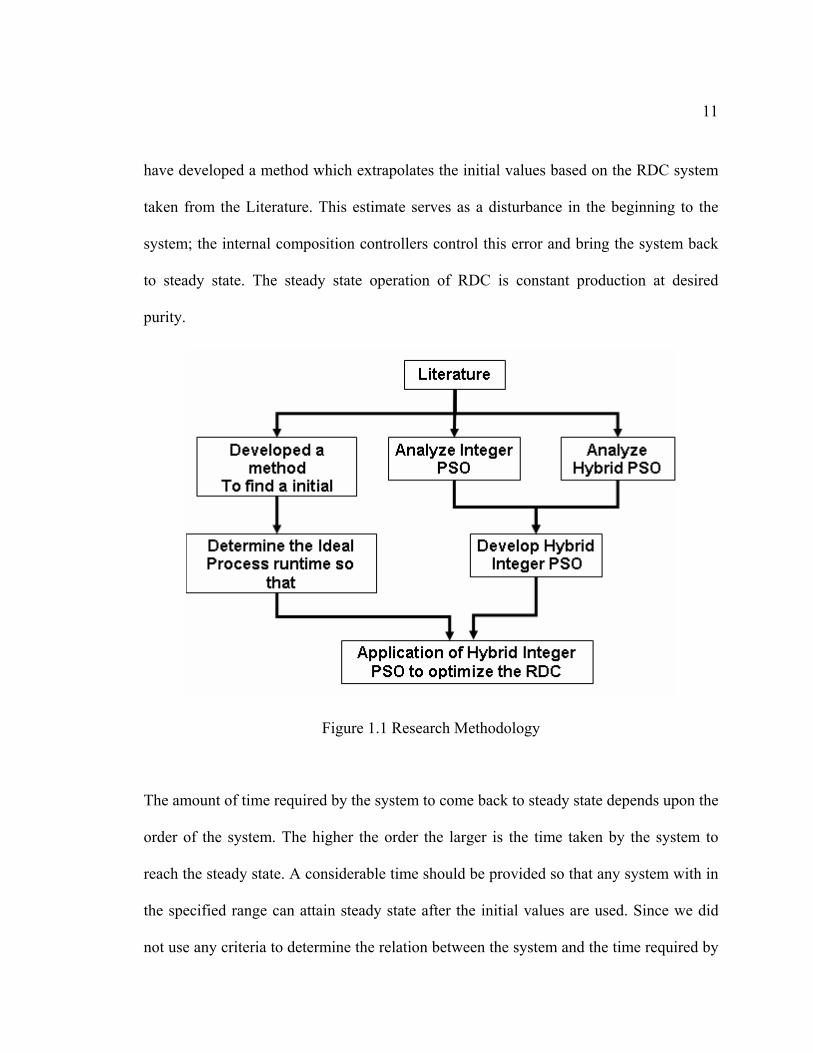
1.4 Research Methodology
Briefly the research methodology can be illustrated as follows:
The Literature was reviewed in search of solution to integer problems then an Integer
PSO model was developed. In order to avoid stagnation and enhance convergence
towards the end of simulations Hybrid version of PSO was selected. The two models
were used for developing a Hybrid-Integer PSO model with some changes. The RDC
Model obtained from the literature is fixed. Any change in optimization Variables would
cause change in the order of the system and the Non-Linear equations describing it. In
order to use such a model an initial estimate of the composition profile is necessary. We
11
have developed a method which extrapolates the initial values based on the RDC system
taken from the Literature. This estimate serves as a disturbance in the beginning to the
system; the internal composition controllers control this error and bring the system back
to steady state. The steady state operation of RDC is constant production at desired
purity.
Figure 1.1 Research Methodology
The amount of time required by the system to come back to steady state depends upon the
order of the system. The higher the order the larger is the time taken by the system to
reach the steady state. A considerable time should be provided so that any system with in
the specified range can attain steady state after the initial values are used. Since we did
not use any criteria to determine the relation between the system and the time required by
12
it to reach steady state, the system was operated for a fixed time long enough so that any
design based on order of the system can attain steady state.
Although there is no guarantee that the system will not blow up it was noticed that
process operation time as large as 16 hours should be sufficient for any system which can
give us desired results to accommodate steady state. There after the Hybrid-Integer PSO
model developed is used as an optimization tool upon the process so as to find the
optimal design based on our requirements.
1.5 Significance
Many chemical industries and petroleum refineries use reactive distillation columns for
separation methods. A huge amount of installation cost is required to setup such a facility
and maintaining it is no exception especially when one of the inputs fed is fuel (oil), mere
mention of the word oil is sufficient to realize how beneficial it is to save even 1% on
fuel expenditures when the consumption is in barrels per day. The rise in cost of fuel day
by day and the ever increasing demand in the production sector of petro-chemicals
necessitate proper efficiency of fuel; one of the requirements in getting the maximum
efficiency out of fuel is the proper design and least consumption to get the maximum
output. This work is another step towards optimizing a process so as to conserve the fuel
intake and thereby save capital.
13
1.6 Contribution
• In this work Hybrid Integer Particle Swarm Optimization (HI-PSO) algorithm
is developed to solve Integer Problems which guarantees faster convergence
and avoids Local Minima Stagnation.
• Implementation of HI-PSO which minimizes fuel consumption in Ideal
Reactive Distillation Column to obtain an optimal design
14
CHAPTER 2
PARTICAL SWAM OPTMIZATION
2.1 The Basic Particle Swarm
The concept of function-optimization by means of a particle swarm was introduced by
James Kennedy, Russel and Eberhart in an IEEE neural network conference paper from
1995 [12]. The method was discovered through simulation of a simplified social model.
In this model, each particle position can be thought of as a state of mind as a particular
setting of the abstract variables that describe our beliefs and attitudes. Movement of
particles in this model then corresponds to the concept of change of mind. Humans adjust
their beliefs to each other; we evaluate stimuli from the environment, compare it to
ourselves, and finally imitate the stimuli. These three important properties of human
social behavior - evaluation, comparison, and imitation - is the main inspiration for the
particle swarm, and the particle swarm utilizes these concepts in adapting to
environmental changes and solving complex and hard problems [11].
Besides being a model of the human social behavior, the particle swarm (as noted by
Kennedy [12] and discussed in chapter 4) is closely related to swarm intelligence. In the
particle swarm, there is no central control no one gives orders. Each particle is a simple
15
agent acting upon local information. Yet, the swarm as a whole is able to perform tasks,
whose degree of complexity is well beyond the capabilities of the individual. The particle
swarm shows signs of self-organization: The interactions among the low-level
components (particles) result in complex structures at the global level (swarm) making it
possible for it to perform optimization of functions.
According to Kennedy, five basic principles define swarm intelligence [11]. First is the
proximity principle: the swarm should be able to carry out simple space and time
computations. Second is the quality principle: the swarm should be able to respond to
quality factors in the environment. Third is the principle of diverse response: the swarm
should not commit its activities along excessively narrow channels. Fourth is the
principle of stability: the swarm should not change its mode of behavior every time the
environment changes. Fifth is the principle of adaptability: the swarm must be able to
change behavior mote when it is worth the computational price. Note that principles four
and five are the opposite sides of the same coin.
The particle swarm seems to adhere to all five principles [12]. Conclusively, the particle
swarm strategies should be thought of a swarm intelligent system. Further, the particle
swarm has roots in artificial life and in evolutionary computation (EC). Indeed, each
particle in the swarm is a simple agent that acts in an environment according to a rule set
16
that takes the state of the environment and the agents into account when deciding what
action to choose, like many artificial life applications.
The connection to evolutionary computation is obvious. The swarm consists of a
population of individuals that represent solutions to the optimization problem, we would
like to solve. Through an iterative and probabilistic modification of these solutions, we
search for an optimal solution. Describing the particle swarm in these EC-terms, the leap
to the evolutionary algorithm is little. The difference between the EA and the PSO with a
simple of view only, how we change the population/swarm from one iteration to the next;
in the EA, genetic operators like selection, crossover and mutation, are used, whereas the
particle in the PSO are modified according to two update formulas that we shall be
familiar with in section 2.1.1
Conceptually, there are, however some differences between the PSO and EA: In PSO
Particles stay alive and inhabit the search space during the run, whereas in EA the
individuals are replaced each generation. Furthermore, the objective is reached through
cooperative search in particle swarms rather than competitive search as in EA.
17
2.1.1 The Algorithm
Next, we present the particle swarm algorithm for optimization of continuous and real-
valued functions in the n-dimensional space, n . The PSO is a population-based search-
algorithm; the population is called a swarm S. The swarm consists of a number of
particles that move around in the search space S. A neighborhood relation N is defined on
the swarm. N determines for all particles pi and pj whether they are neighbors or not, and
we can thus for each particle p assign a neighborhood, N(p), containing all neighbors of
p. A fitness function f must be defined to compare candidate solutions in the search space
S, which is a subset of n , and map into the real numbers, i.e.: : nf S ⊆ → . In fact,
the PSO only compares fitness, so an ordinal fitness function would suffice. Each particle
p has two state variables:
• Its current position: ( )x t ,
• Its current velocity: ( )v t ,
As well as a small memory containing:
• Its best position: ( )p t , and
• The best ( )p t of all ( ) : ( )p N p g t∈ ,
Where ( )p t , ( )g t , ( )x t and ( )v t are n-dimensional vectors.
18
Particle Swarm Optimization consists of three parameters basically: maxv , which restricts
every coordinate of ( )v t within the range [- maxv to maxv ] and 1φ and 2φ that determine the
influence of ( )p t and ( )g t in the velocity update formula.
The swarm is initialized at time t = 0 by placing the particles randomly and uniformly
distributed in S and assigning a random and uniformly chosen velocity vector (0)v from
Vn. moreover, we set (0)p = (0)g = (0)x .
The iterative optimization process starts after this initialization. The expressions for the
particle positions and velocities in the next time step are given by these recursive
equations:
( ) ( )1 2( 1) ( ) ( ) ( ) ( ) ( )v t v t p t x t g t x tφ φ+ = + − + − (2.1)
( 1) ( ) ( 1)x t x t v t+ = + + (2.2)
The position of a particle at time t+1 is calculated as a sum of it old position ( )x t and
current velocity ( 1)v t + . Additionally, the velocity ( 1)v t + is updated as a sum of the
particle's old velocity ( )v t , its own cognitive learning part ( )1 ( ) ( )p t x tφ − and social
learning part ( )2 ( ) ( )g t x tφ − .
19
After having calculated the velocities and position for the next time step t+1, the first
iteration of the algorithm is completed. Typically, this process is iterated for a certain
number of time steps, or until some acceptable solution has been found by the algorithm.
Here we present the pseudo-code for the PSO algorithm. During the search, the Particles
exchange information about their positions and fitness values. This communication
results in, that the swarms learn and refine its knowledge about the search, and move
towards the good search space areas. This is analogous to flocks of birds flying and
searching for food, to social insects such as bees and ants when foraging or nesting, and
to humans that affect the minds of each other by interacting socially.
Program Particle Swarm Optimization Algorithm
Set t = 0;
Initialize 1φ , 2φ ,Vmax and define N;
:p S∀ ∈ Initialize ( )x t , ( )v t , ( )p t , ( )g t as described;
While {Min. is not reached or Iterations not exhausted
:p S∀ ∈ Calculate ( 1)v t + and ( 1)x t + using 1 and 2
:p S∀ ∈ Update ( 1)p t + with ( 1)x t + if ( )( 1)f x t + is better than ( )( )f x t
:p S∀ ∈ Update ( 1)g t + with ( 1)p t + in N(p)
}
20
These analogies in nature of refinement of knowledge by cooperation have been the
inspiration for the PSO. Therefore, as an emergent result of the two simple equations (1)
and (2) above, the swarm as a whole will identify and approach the good areas of the
search space in a self-organized structure based on comparison to and imitation of each
other.
On the algorithmic level, the main strength of the PSO is its fast convergence, which
compares favorable to many EA implementations. However, it has three major eaknesses:
• It cannot dynamically adjust its velocities when fine-tuning a found optimum,
and hence the convergence rate decreases dramatically in the close vicinity of
optima [13].
• On hard problem for instance with many optima, its fast convergence rate
often results in premature convergence [14].
• The number of PSO parameters to tune is critically big [14]
Next we describe extensions that deal with the first two issues, and in the following
section we discuss the matter of parameter selection in the PSO.
21
2.2 Extensions to the Particle Swarm
2.2.1 Controlling the Convergence
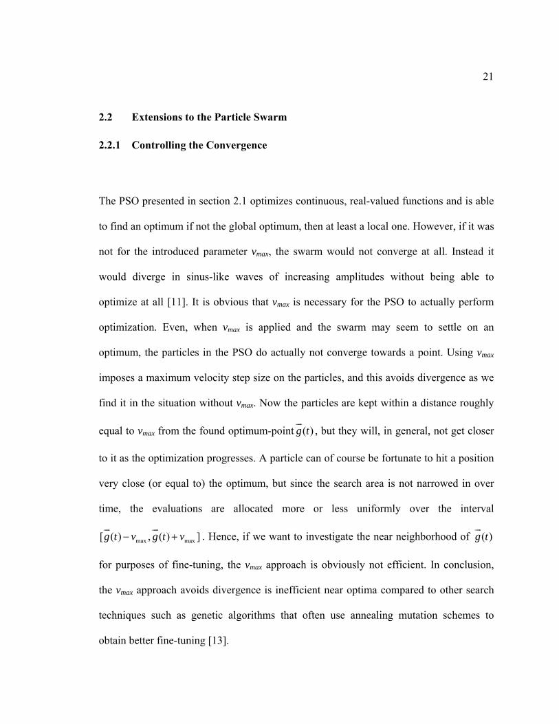
The PSO presented in section 2.1 optimizes continuous, real-valued functions and is able
to find an optimum if not the global optimum, then at least a local one. However, if it was
not for the introduced parameter vmax, the swarm would not converge at all. Instead it
would diverge in sinus-like waves of increasing amplitudes without being able to
optimize at all [11]. It is obvious that vmax is necessary for the PSO to actually perform
optimization. Even, when vmax is applied and the swarm may seem to settle on an
optimum, the particles in the PSO do actually not converge towards a point. Using vmax
imposes a maximum velocity step size on the particles, and this avoids divergence as we
find it in the situation without vmax. Now the particles are kept within a distance roughly
equal to vmax from the found optimum-point ( )g t , but they will, in general, not get closer
to it as the optimization progresses. A particle can of course be fortunate to hit a position
very close (or equal to) the optimum, but since the search area is not narrowed in over
time, the evaluations are allocated more or less uniformly over the interval
max max[ ( ) , ( ) ]g t v g t v− + . Hence, if we want to investigate the near neighborhood of ( )g t
for purposes of fine-tuning, the vmax approach is obviously not efficient. In conclusion,
the vmax approach avoids divergence is inefficient near optima compared to other search
techniques such as genetic algorithms that often use annealing mutation schemes to
obtain better fine-tuning [13].
22
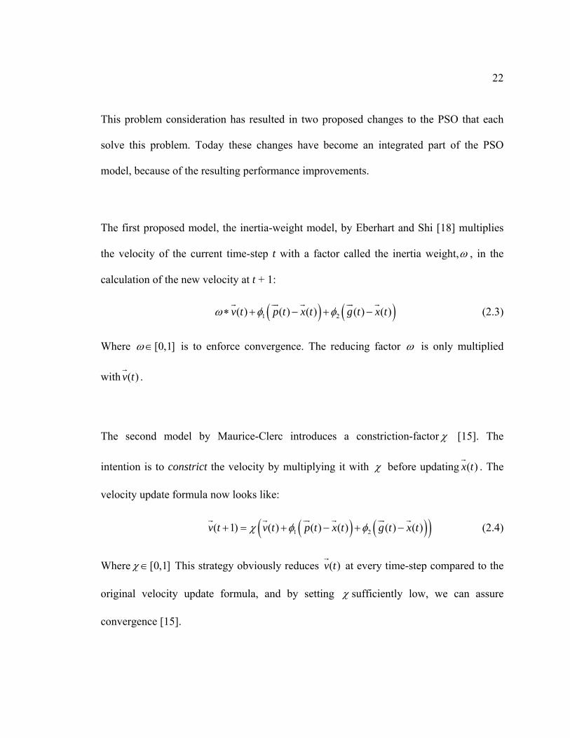
This problem consideration has resulted in two proposed changes to the PSO that each
solve this problem. Today these changes have become an integrated part of the PSO
model, because of the resulting performance improvements.
The first proposed model, the inertia-weight model, by Eberhart and Shi [18] multiplies
the velocity of the current time-step t with a factor called the inertia weight,ω , in the
calculation of the new velocity at t + 1:
( ) ( )1 2( ) ( ) ( ) ( ) ( )v t p t x t g t x tω φ φ∗ + − + − (2.3)
Where [0,1]ω∈ is to enforce convergence. The reducing factor ω is only multiplied
with ( )v t .
The second model by Maurice-Clerc introduces a constriction-factor χ [15]. The
intention is to constrict the velocity by multiplying it with χ before updating ( )x t . The
velocity update formula now looks like:
( ) ( )( )1 2( 1) ( ) ( ) ( ) ( ) ( )v t v t p t x t g t x tχ φ φ+ = + − + − (2.4)
Where [0,1]χ ∈ This strategy obviously reduces ( )v t at every time-step compared to the
original velocity update formula, and by setting χ sufficiently low, we can assure
convergence [15].
23
It is easy to realize that the two modifications of the velocity update formula are in effect
equivalent: The constriction-factor can mimic the inertia-weight, and vice versa: if we
have a setting of 1 2( , , ) ( , , )x y zχ φ φ = in the constriction model, we obtain an equivalent
setting in the inertia-weight model by setting 1 2( , , ) ( , , )x xy xzω φ φ = . Thus, to transfer
settings between the two models it suffices to multiply (or respectively divide) 1φ and 2φ
with the value of χ .
2.2.2 Avoiding Premature Convergence
In this section we present extensions to the PSO model that is concerned with the
problem of premature convergence to sub-optimal solutions. They do not only manipulate
the velocity update formula, but build up a genuinely new model on the swarm level. The
PSO model converges by nature rather quickly (i.e. the diversity in the swarm decreases
quickly). This is exact, what is wanted when the problem in question is easy e.g. is a uni-
modal problem. On such easy problems, the convergence should be as fast as possible,
because there is no risk of being trapped on a sub-optimal solution. However, when we
face more difficult, multi-modal problems, then too fast convergence often becomes
inadequate and unwanted. When there are many different local optima, we must spend
more time on investigating different solution areas before converging simply to avoid
getting stuck in a sub-optimal area; i.e. to avoid premature convergence.
24
This topic has been addressed in several papers. The hybrid-PSO model by Løvbjerg and
colleagues uses breeding between particles and sub-populations [16]. Since breeding is a
core element in the GA, the authors hypothesize that a PSO with breeding might reach a
better optimum. Breeding is implemented through arithmetic crossover as known from
GAs; a parameter pb is introduced to control the probability of breeding. Further,
offspring replace parents, and the population is divided into sub-populations to avoid
premature convergence. Finally, a parameter psb was added to control the probability of
breeding inside sub-populations. Based on their research, the authors conclude that
marginally faster convergence is obtained with the hybrid-PSO, and that the best found
values are better on multi-modal problems but worse on uni-modal. This model has been
explained in upcoming section and this forms the basis of our Modified Algorithm.
2.2.3 Speeding up Convergence
The issue of speeding up convergence towards optimum has not been thoroughly
investigated yet. The primary reason for this is that precisely the convergence speed of
the swarm is already an inherent force of the PSO construction as discussed by Angeline
[13]. Hence, the PSO converges to the fitness optimum quickly on easy problems, but is
also more vulnerable to premature convergence on multi-modal problems. With ω and
χ added to the algorithm, the rapid convergence even lasts throughout the whole
optimization process so fine-tuning of solutions is efficient. Obtaining fast convergence
25
has therefore in much research therefore been reduced to tuning ω and χ , rather than
creating mechanisms that changes the fundamental behavior of the particles.
Kennedy and colleagues present a model that tries to improve particles trajectories [11].
He first approximates a number C of cluster-centers. The idea is that these centers might
be nearer to the optimum (around which the particles are swarming), than the particles
themselves, and thus substituting these centers for ( )p t and ( )g t might improve their
search. This approach tries to improve the convergence within sub-clusters, which leads
to faster convergence towards the fitness optimum. Since the convergence rate in only
increased within clusters (that will converge anyway), this model has the nice property
that it tries to improve the convergence rate towards good solutions without increasing
the risk of converging on sub-optimal solutions. Substitutions of ( )p t only, of ( )g t only,
and of both are tested. The author concluded that average performance per fixed number
of iterations can be improved by substituting, but the results are only preliminary.
2.3 Parameter Selection
With the introduction of the inertia weight and the constriction factor as fundamental
concepts of the PSO, there is quite a number of parameters to consider in the PSO-
26
algorithm: ω , χ , 1φ , 2φ and vmax: Thus, at this point it might be a good idea to take a
look at how the parameters should be controlled in the PSO model.
The parameter-settings of the PSO determine how it optimizes the search-space. For
instance, one can apply a general setting that gives reasonable results on most problems,
but seldom is very optimal. A useful setting for a general search is to set 1 2 2φ φ= = and
the inertia weight ω = 0:8. The value of vmax depends on the size of S (and properties of
the function being optimized), but for practical use vmax is often set to approximately.
10% of the average dimension size of S.
But these settings cannot be used on many problems with optimal success; hence we must
have knowledge of the effects of the different settings, so we can pick a suitable setting
from problem to problem. For instance, if the problem for which we are optimizing has a
uni-modal fitness-landscape, we most likely want the PSO to act as a hill-climber, and we
can set the parameters in a specific way to support an efficient hill-climbing behavior. In
contrast, in other cases where the fitness landscape has many peaks, we can set the
parameters differently to adapt the behavior to multi-modal problem-domains.
27
2.3.1 The Control Parameters 1φ and 2φ
There are two important facts to consider, when setting 1φ and 2φ .The first fact is that the
relation between the two values decides the point of attraction, which is given by:
1 2
1 2
( ) ( )p t g tφ φφ φ++
If 1 2φ φ>> , the particle p will be much more attracted to the best found position by itself,
( )p t , rather than the best position found by the neighborhood ( )g t , and vice versa if
1 2φ φ< .
The extreme case 2φ = 0 converts all particles to independent hill-climbers since the
social learning part ( )2 ( ) ( )g t x tφ − is 0. The iterated hill-climber finds the best point in
the neighborhood by replacing the current point, if a better is found. This is repeated until
a local optimum is reached, and the whole process can in addition be repeated with new
starting points as many times as one wishes. Similarly, the PSO with setting 2φ = 0
swarms about the point ( )p t , and searches a neighborhood, whose size is indirectly
defined by vmax. If the particle finds a better solution (and this will eventually happen if
( )p t is not already equal to the optimum) ( )p t will be updated, and the particle will start
swarming around the updated ( )p t . Conclusively, the particle (precisely as the hill-
28
climber) moves uphill, and this process continues iteratively until an optimum is found,
in accordance with the behavior of a hill-climber). Conversely, the hill-climber particle
in the PSO does not know exactly when the optimum is found, because it does not
systematically (exhaustively) search the neighborhood.
In the other extreme case, where 1φ = 0, the particle own cognitive learning part
( )1 ( ) ( )p t x tφ − is 0, and the whole swarm is attracted to one single point only,
namely ( )g t . Essentially, the swarm now turns into one big hill-climber as described
above; all particles swarm around ( )g t , and moves with each update of ( )g t . The
neighborhood is searched in parallel by all the particles simultaneously, and resulting in
one parallel, stochastic hill-climber.
If 1 2φ φ= , each particle will be attracted to the average of ( )p t and ( )g t . Since 1φ
expresses how much the particle trusts its own past experience, it is called the cognitive
parameter, and since 2φ expresses how much it trusts the swarm, it is called the social
parameter. Most implementations use a setting with 1φ roughly equal to 2φ . However,
Carlisle and Dozier [17] reported good results with 1φ = 2:8 and 2φ = 1:3 [17].
29
The second fact to consider when setting the control variables is the magnitudes of 1φ
and 2φ . The higher 1φ and 2φ the more acceleration the particles can obtain. In fact, at
any time a particle's acceleration is given by the term: ( ) ( )1 2( ) ( ) ( ) ( )p t x t g t x tφ φ− + −
(Without inertia-weight or constriction). Thus, setting the control variables high, enables
the swarm to react rapidly to changes in the search, whereas if they are set low, the
particles will react slowly and move in waves of huge-magnitude and low-frequency.
They generally move farther away from the point of attraction 1 2
1 2
( ) ( )p t g tφ φφ φ++
and will
not change direction as often as with the control variables set high.
2.3.2 The Inertia Weight ω
The inertia weight ω controls the momentum of the particle: If ω << 1, only little
momentum is preserved from the previous time-step; thus quick changes of direction are
possible with this setting. The concept of velocity is completely lost if ω = 0, and the
particle then moves in each step without knowledge of the past velocity. On the other
hand, if ω is high (> 1) we get the same effect as when 1φ and 2φ are low: Particles can
hardly change their direction and turn around, which of course implies a larger area of
exploration as well as a reluctance against convergence towards optimum. Setting ω > 1
must be done with care, since velocities are further biased for an exponential growth.
30
This setting is rarely seen in PSO implementation, and always together with vmax. In
short, high settings near 1 facilitate global search, and lower settings in the range [0:2;
0:5] facilitate rapid local search.
R. Eberhart and Y. Shi have studied ω in several papers and found that when vmax is not
small (≥ 3), an inertia-weight of 0.8 is a good choice [18]. Although this statement is
solely based on a single test function, the Schaffer function, this setting actually is a good
choice in many cases. The authors have also applied an annealing scheme for the ω -
setting of the PSO, where ω decreases from ω = 0.9 to ω = 0.4 over the whole run [19].
They compared their annealing scheme results to results with ω = 1 obtained by
Angeline [13], and conclude a significant performance improvement on the four tested
functions. The decreasing ω -strategy is a near-optimal setting for many problems, since
it allows the swarm to explore the search-space in the beginning of the run, and still
manages to shift towards a local search when fine-tuning is needed.
2.3.3 The Constriction Factor χ
The constriction factor model has as mentioned in section 2.2.1 the same effect asω ,
except that it also scales the contributions from ( )p t and ( )g t with χ . Thus, any
regulation of the ability to change direction (i.e. the relationship between ( )v t and
31
( ) ( )1 2( ) ( ) ( ) ( )p t x t g t x tφ φ− + − must be done with 1φ and 2φ with this model. However,
basically χ acts as ω : Low values facilitates rapid convergence and little exploration
where as high values gives slow convergence and much exploration.
One of the few theoretical founded contributions to particle swarm research comes from
the mathematician Maurice Clerc, who has proposed the constriction factor [15]. He has
studied the particle swarm system by means of second order differential equations. In
doing so, it is possible to determine under which conditions the swarm will converge.
However, we must emphasize that this analysis did not model a swarm of particles, but
only one single deterministic particle in a one-dimensional space. Further, the author
assumed a static ( )p t and ( )g t . In spite of these simplifications, it is worth looking at one
particular outcome of the analysis. In the constriction model we can set χ as a function
of 1φ and 2φ , so that convergence is ensured even without vmax. An additional parameter
k, which controls the convergence speed of the particles to the point of attraction, is
introduced instead of  (see eq. 5).
( )2
2 4
kχφ φ φ
=− − −
where 1 2 4, [0,1]kφ φ φ= + ≥ ∈ (2.5)
32
The supposed advantage of this shift from χ to k, is that k more clearly and reliably can
control swarm behavior: If k is close to 0, we get fast convergence (almost hill-climbing
behavior), and if k is near 1 we get the slowest possible convergence with a high degree
of exploration, which is desired for strongly multimodal problems.
2.3.4 The Maximum Velocity vmax
Originally, vmax was introduced to avoid explosion and divergence. With χ or ω in the
update formula, vmax to some degree has become unnecessary; at least convergence can be
assured without it [15]. Thus, some researchers simply do not use vmax. In spite of this
fact, the maximum velocity limitation can still improve the search. For instance, if a
particle is positioned in one end of the search-space and ( )p t and ( )g t in the other end,
the particle will be able to obtain a velocity of four times i.e. If the distance, d, from ( )x t
to ( )p t and ( )g t is approximately the length of the search space, and we assume
1 2 2φ φ≈ ≈ , then from eq. (2.1) we get that ( 1) 4v t d+ ≈ i.e. four times the size of the
search space, which obviously is nonsense. Hence, after moving to the other end of the
search-space, in what probably is one timestep, the particle will now have to spend time
(and evaluations) decelerating its velocity before being able to turn around. In this period
the search is more or less locked up, and still the PSO uses CPU-time on evaluating the
33
same boundary solutions again and again. Alternatively, it could have approached the
point of attraction.
1 2
1 2
( ) ( )p t g tφ φφ φ++
(2.6)
In a controlled and more efficient manner with a suitable vmax applied, thus gaining useful
information about the fitness landscape between the two corners by sampling different
solutions on its way across the search space.
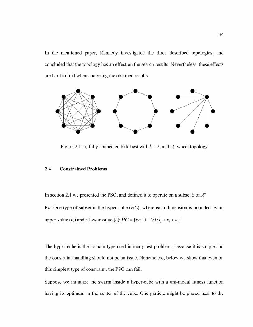
2.3.5 The Neighborhood Topology
Another important factor in PSO is the neighborhood topology. The PSO presented in
2.1.1, implicitly uses a so-called fully connected neighborhood topology (or gbest). Every
particle is neighbor of every other particle. In a paper by Kennedy, other topologies are
described as well [14]:
• The k-best topology, which connects every particle to its k nearest particles in
the topological space. With k = 2, this becomes the circle topology (and with k
= swarmsize-1 it becomes a gbest topology).
• The wheel topology, in which the only connections are from one central
particle to the others (see figure). In addition, one could magine a huge
number of other topologies.
34
In the mentioned paper, Kennedy investigated the three described topologies, and
concluded that the topology has an effect on the search results. Nevertheless, these effects
are hard to find when analyzing the obtained results.
Figure 2.1: a) fully connected b) k-best with k = 2, and c) twheel topology
2.4 Constrained Problems
In section 2.1 we presented the PSO, and defined it to operate on a subset S of n
Rn. One type of subset is the hyper-cube (HC), where each dimension is bounded by an
upper value (ui) and a lower value (li): { | : }ni i iHC x i l x u= ∈ ∀ < <
The hyper-cube is the domain-type used in many test-problems, because it is simple and
the constraint-handling should not be an issue. Nonetheless, below we show that even on
this simplest type of constraint, the PSO can fail.
Suppose we initialize the swarm inside a hyper-cube with a uni-modal fitness function
having its optimum in the center of the cube. One particle might be placed near to the
35
center in all dimensions except in one dimension, where it is very near the boundary. We
call this dimension b. Being relatively close to the global optimum, it might get the best
fitness value of all particles. Further, let us assume that its velocity vb(t) points towards
the border in this dimension b such that xb(t) crosses the border in the next timestep.
Following the standard PSO implementation of domain-border violations, we adjust the
coordinate-value to lie on the border: xb(t) = ub (or lb).
As long as this particle's fitness is not lower than any of the others, two things will
happen:
• xbt will remain equal to ub, because pb(t) and gb(t) also are equal to xb(t), and
thus the velocity vb(t) will continue to point outwards of the search-space.
• The b'th coordinate of the other particles will be attracted to xb(t), and sooner
or later they will end up with the value ub. If this happens before a new gb(t) is
found by another particle, the b'th coordinate of all the particles will be stuck
at ub forever.
This problem can be avoided by simply allowing the particles to move outside the search
space S, but without evaluating outside the search space. As a particle cannot improve its
fitness being outside, ( )p t and ( )g t are always updated inside S, and after some time the
particle will enter S again because of the attraction to exactly ( )p t and ( )g t . This scheme
can be improved even further.

36
To conclude particle Swarm optimization in its basic form although is very simple but
may suffer from inabilities to reach the global minima. Few modifications need to be
done, although these modifications like, inertia weight, neighborhood, constriction factor
and the Vmax operator have become an intrinsic part of the algorithm, there is still room
for development when coming to specific problems.
37
CHAPTER 3
HYBRID INTERGER PSO
In this chapter we develop the Hybrid-Integer PSO model based on the existing
extensions to particle Swarm Optimization, The integer PSO and the Hybrid-PSO. In
section 3.1.1 we discuss in detail the Hybrid particle Swarm optimization, Followed by
integer programming of Particle Swarm Optimization in section 3.1.2. In section 3.2 the
shortcoming of both the algorithms are discussed and the need to amalgamate them so as
to bring a more hybridized version of Integer PSO is put forward. The chapter is
concluded by testing some standard integer test problems.
3.1 Background
3.1.1 Hybrid PSO
Hybrid Particle Swarm Optimizers is combining the idea of the particle swarm with
concepts from Evolutionary Algorithms. The hybrid PSO combines the traditional
velocity and position update rules with the ideas of breeding and subpopulations. PSO
with breeding strategies have the potential to achieve faster convergence and the potential
to find a better solution. Both Eberhart [11] and Angeline[13] conclude that hybrid
models of the standard GA and the PSO could lead to further advances. Lovberg et al.
38
present such a hybrid model [16]. The model incorporates one major aspect of the
standard GA into the PSO, the reproduction. In here we will refer to the used
‘reproduction’ and ‘recombination’ of genes only as “breeding”. Breeding is one of the
core elements that make the standard GA, a powerful algorithm. In addition to breeding
Lovberg et al. introduce a hybrid with both breeding and subpopulations. Subpopulations
have previously been introduced to standard GA models mainly to prevent premature
convergence to suboptimal points [37]. The motivation for this extension was that the
PSO models, including the hybrid PSO with breeding, may also reach suboptimal
solutions. Breeding between particles in different sub-populations was also added as an
interaction mechanism between subpopulations.
The particles have no neighborhood restrictions, meaning that each particle can affect all
other particles. This neighborhood is of type star (fully connected network), which have
been shown to be a good neighborhood type in [14]. The structure of the hybrid model is
illustrated.
Start Initialize PSO while ( Termination Criteria not Satisfied) do
Start PSO Evaluate Calculate new velocity vectors Update Positions Breed
End} end
39
The breeding is done by first determining which of the particles that should breed. This is
done by iterating through all the particles and, with probability pb ( breeding probability),
mark a given particle for breeding. Note that the fitness is not used when selecting
particles for breeding. From the pool of marked particles we now select two random
particles for breeding. This is done until the pool of marked particles is empty. The parent
particles are replaced by their offspring particles, thereby keeping the population size
fixed.
The position of the offspring is found for each dimension by arithmetic crossover on the
position of the parents, i.e.,
Child1(xi)=pi*parent1(xi)+ (1-pi)*parent2(xi) (3.4)
Child2(xi)=pi*parent2(xi)+ (1-pi)*parent1(xi) (3.5)
Where pi is a uniformly distributed random value between 0 and 1. The velocity vector of
the offspring is calculated as the sum of the velocity vectors of the parents normalized to
the original length of each parent velocity vector.
1 21 1
1 2
( ) ( )( ) ( )( ) ( )
parent v parent vchild v parent vparent v parent v
+=
+ (3.6)
1 22 2
1 2
( ) ( )( ) ( )( ) ( )
parent v parent vchild v parent vparent v parent v
+=
+ (3.7)
40
The arithmetic crossover of positions and velocity vectors used were empirically tested to
be the most promising. The arithmetic crossover of positions in the search space is one of
the most commonly used crossover methods with standard real valued GA’s, placing the
offspring within the hypercube spanned by the parent particles. The main motivation
behind the crossover is that offspring particles benefit from both parents. In theory this
allows good examination of the search space between particles. Having two particles on
different suboptimal peaks breed could result in an escape from a local optimum, and
thus aid in achieving a better one. We used the same idea for the crossover of the velocity
vector. Adding the velocity vectors of the parents results in the velocity vector of the
offspring. Thus each parent affects the direction of each offspring velocity vector equally.
In order to control that the offspring velocity was not getting too fast or too slow, the
offspring velocity vector is normalized to the length of the velocity vector of one of the
parent particles. Finally, the starting position of a new offspring particle is used as the
initial value for this particle’s best found optimum ( )ip t .
The motivation for introducing subpopulations is to restrict the gene flow (keeping the
diversity) and thereby attempt to evade suboptimal convergence. The subpopulation
hybrid PSO model is an extension of the just described breeding hybrid PSO model. In
this new model the particles are divided into a number of subpopulations. The purpose of
the subpopulations is that each subpopulation has its own unique best known optimum.
The velocity vector of a particle is updated as before except that the best known position
41
( ( )ig t in the formula) now refers to the best known position within the subpopulation that
the particle belongs to. In terms of the neighborhood topology suggested by Kennedy in
[14], each subpopulation has its own neighborhood. The only interaction between
subpopulations is if parents from different subpopulations breed. Breeding is now
possible both within a subpopulation but also between different subpopulations. An extra
parameter called probability of same subpopulation breeding (psb) determines whether a
given particle selected for breeding is to breed within the same subpopulation (probability
psb), or with a particle from another subpopulation (probability 1- psb ). Replacing each
parent with an offspring particle ensures a constant subpopulation size.
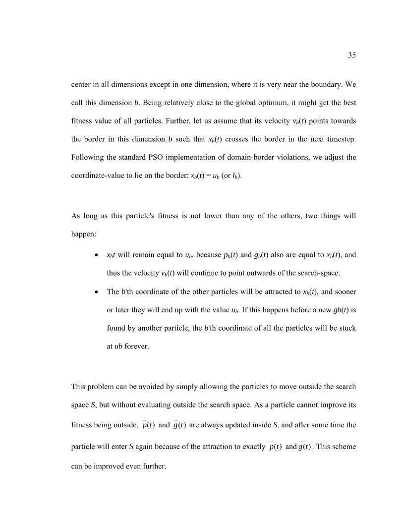
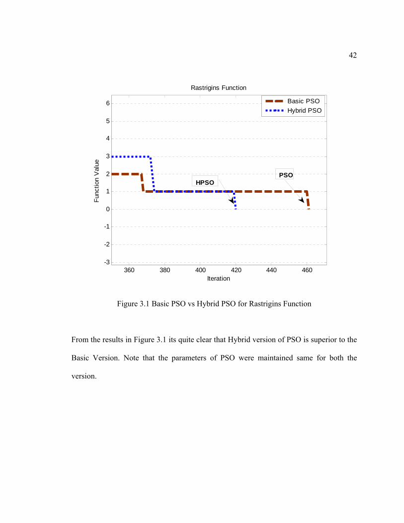
As an example we take a function 2
1( ) ( 10cos(2 ) 10)
n
i ii
F x x xπ=
= − +∑ which is generally
called Rastrigins Function. It has a global minimum of zero and has the bounds in the
range [ 5.12,5.12]x∈ − , ( ) 0F x = . The PSO parameters were as follows:
The maximum number of allowed function evaluations was set to 10000 (500 iterations);
the desired accuracy was 100%; the constriction factor was set equal to 1; the inertia
weight ω was gradually decreased from 0.7 towards 0.4; c1 = c2 = 2; and Vmax = 100 and
the size of the Swarm were selected to be equal to 20.
42
360 380 400 420 440 460-3
-2
-1
0
1
2
3
4
5
6
Iteration
Func
tion
Val
ueRastrigins Function
Basic PSOHybrid PSO
HPSOPSO
Figure 3.1 Basic PSO vs Hybrid PSO for Rastrigins Function
From the results in Figure 3.1 its quite clear that Hybrid version of PSO is superior to the
Basic Version. Note that the parameters of PSO were maintained same for both the
version.
43
3.1.2 Integer PSO
A wide variety of problems can be represented as discrete optimization models. An
important area of application concerns the efficient management of a limited number of
resources so as to increase productivity and/or profit. Such applications are encountered
in Operational Research problems such as goods distribution, production scheduling, and
machine sequencing. There are applications in mathematics to the subjects of graph
theory and logic [27].
Statistical applications include problems of data analysis and reliability. Recent scientific
applications involve problems in molecular biology, high energy physics and x-ray
crystallography. A political application concerns the division of a region into election
districts [27]. Capital budgeting, portfolio analysis, network and VLSI circuit design, as
well as automated production systems are some more applications in which Integer
Programming problems are met [27].
Yet another, recent, and promising application is the training of neural networks with
integer weights, where the activation function and weight values are confined in a narrow
band of integers. Such neural networks are better suited for hardware implementations
compared to real weight ones [28].
44
The Unconstrained Integer Programming problem can be defined as
min ( ), n
xf x x S∈ ⊆ (3.1)
Where Z is the set of integers, and S is a not necessarily bounded set, which is considered
as the feasible region. Maximization of Integer Programming problems is very common
in the literature, but we will consider only the minimization case, since a maximization
problem can be easily transformed to a minimization problem and vice versa. The
problem defined in Eq. (3.1) is often called “All Integer Programming Problem", since all
the variables are integers, in contrast to the “Mixed Integer Programming Problem",
where some of the variables are real.
Optimization techniques developed for real search spaces can be applied on Integer
Programming problems and determine the optimum solution by rounding off the real
optimum values to the nearest integer [27], [29].
Evolutionary and Swarm Intelligence algorithms are stochastic optimization methods that
involve algorithmic mechanisms similar to natural evolution and social behavior
respectively. They can cope with problems that involve discontinuous objective functions
and disjoint search spaces [30], [11], [32]. Genetic Algorithms (GA), Evolution
Strategies (ES), and the Particle Swarm Optimizer (PSO) are the most common
paradigms of such methods. GA and ES draw from principles of natural evolution which
are regarded as rules in the optimization process. On the other hand, PSO is based on
45
simulation of social behavior. Early approaches in the direction of Evolutionary
Algorithms for Integer Programming are reported in [34], [35]. In GA, the potential
solutions are encoded in binary bit strings. Since the integer search space, of the problem
defined in Eq. (3.1), is potentially not bounded, the representation of a solution using a
fixed length binary string is not feasible [33]. Alternatively, ES can be used, by
embedding the search space Zn into Rn and truncating the real values to integers.
However, this approach is not always efficient due to the existence of features of ES,
which contribute to the detection of real valued minima with arbitrary accuracy. These
features are not always needed in integer spaces, since the smallest distance of two
points, in 1-norm, is equal to 1 [33].
In Integer-PSO the velocity of the particles and the Swarm positions are updated as per
the standard equations mentioned in the previous chapter. Integer Programming test
problem was selected to investigate the performance of the PSO method. Each particle of
the swarm was truncated to the closest integer, after the determination of its new velocity
using
( ) ( ) ( )1 2 3( 1) ( ) ( ) ( ) ( ) ( ) ( ) ( )v t v t p t x t g t x t n t x tω φ φ φ+ = ∗ + − + − + − (3.2)
And positions using
( 1) ( ) ( 1)x t x t v tχ+ = + + . (3.3)
46
As an example
35 20 10 32 1020 40 6 31 32
( ) (15 27 36 18 12) 10 6 11 6 1032 31 6 38 2010 32 10 20 31
TF x x x
− − −⎛ ⎞⎜ ⎟− − −⎜ ⎟⎜ ⎟= − + − − − −⎜ ⎟
− − −⎜ ⎟⎜ ⎟− − −⎝ ⎠
The range of x is [ 100,100]x∈ − and the solutions is ( ) 737F x = − with
(0,11,22,16,6) (0,12,23,17,6)x and x= = [39]
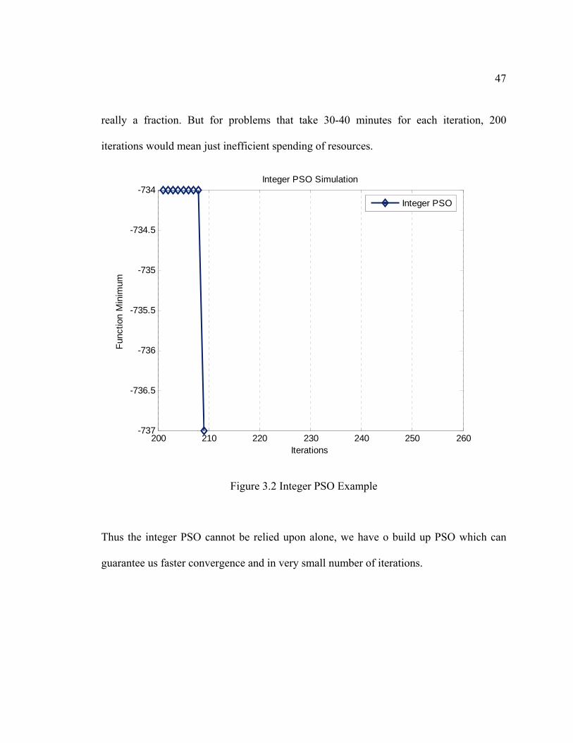
In the above example of optimization, the maximum number of allowed function
evaluations was set to 25000 i.e. 1250 iterations, desired accuracy was 100%,
neighborhood acceleration (c3) set to 1, constriction factor was set to 0.729; the inertia
weight ω was gradually decreased from 1 towards 0.1 with c1 = c2 = 2, Vmax = 4 and the
size of the Swarm were selected to be 20. The range of variables was bounded between [-
100 to 100]. The aforementioned values for all PSO parameters are considered default
values, and they are used widely in the relevant literature [11].
The results in Figure 3.2 indicate that using the Integer PSO for optimization of Integer
problems can give solutions to Integer based problems. As can be seen Integer PSO takes
205 iterations to reach the global minimum of -737.the number of iterations taken by
integer PSO is indeed high. Since this is a very simple example, the amount of time is
47
really a fraction. But for problems that take 30-40 minutes for each iteration, 200
iterations would mean just inefficient spending of resources.
200 210 220 230 240 250 260-737
-736.5
-736
-735.5
-735
-734.5
-734
Iterations
Func
tion
Min
imum
Integer PSO Simulation
Integer PSO
Figure 3.2 Integer PSO Example
Thus the integer PSO cannot be relied upon alone, we have o build up PSO which can
guarantee us faster convergence and in very small number of iterations.
48
3.2 Hybrid-Integer PSO
In the previous section it has been shown that Hybrid PSO is superior to Basic
PSO with all modifications. Since the problem surrounding our Process (RDC) involves
variables which are pure integers, it is of prime importance that the PSO algorithm should
be able to converge onto a satisfactory integer value for any problem which is discrete in
nature. As a test to the Hybrid-PSO, we have chosen a fitness function cited in the
literature [29] to check whether hybrid PSO can converge to optimal integer solution.
• As an example, 2 21 2 1 2 1 2( ) 2 3 4 6 3F x x x x x x x= + + − − with range for x as
[ 100,100]x∈ − and solution ( ) 6F x = − at (2, 1)x = −
As can be seen from the Figure 3.3 both the standard PSO and the Hybrid PSO fail to
converge to the required Global minimum. Thus it is necessary to amalgamate Integer
PSO as discussed in section 3.1.1 with Hybrid PSO 3.1.2. Thus we came up with our
Algorithm termed HI-PSO (Hybrid-Integer PSO).
In HI-PSO the initial Swarm size is incremented to large size compared to its actual size
and the Integer PSO is operated upon this Swarm. After the evaluation of the fitness
function the best swarms are selected out of the total flock of swarms that was created in
the beginning. The criterion of selection is the fitness achieved for the particular function.
After the selection rest of Swarm is neglected. This is like ‘Selection or ‘Survival of the
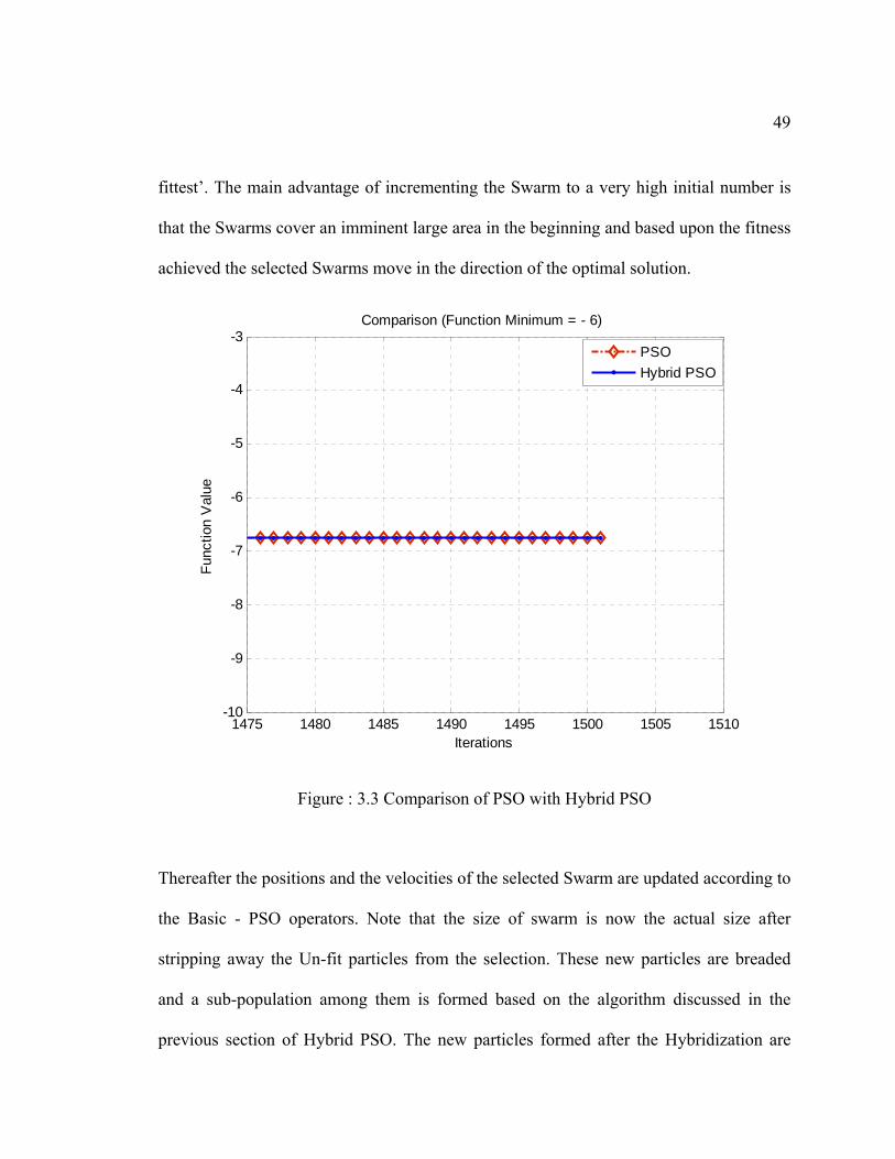
49
fittest’. The main advantage of incrementing the Swarm to a very high initial number is
that the Swarms cover an imminent large area in the beginning and based upon the fitness
achieved the selected Swarms move in the direction of the optimal solution.
1475 1480 1485 1490 1495 1500 1505 1510-10
-9
-8
-7
-6
-5
-4
-3
Iterations
Func
tion
Val
ue
Comparison (Function Minimum = - 6)
PSOHybrid PSO
Figure : 3.3 Comparison of PSO with Hybrid PSO
Thereafter the positions and the velocities of the selected Swarm are updated according to
the Basic - PSO operators. Note that the size of swarm is now the actual size after
stripping away the Un-fit particles from the selection. These new particles are breaded
and a sub-population among them is formed based on the algorithm discussed in the
previous section of Hybrid PSO. The new particles formed after the Hybridization are
50
rounded to the nearest integers and then they are evaluated by the function and the fitness
or termination criterion is tested. If it is satisfied the algorithm stops other wise the
algorithm repeats going back to hybridization-rounding step and re-evaluated until the
termination criterion is met.
• As a test we recall the previous example 2 21 2 1 2 1 2( ) 2 3 4 6 3F x x x x x x x= + + − − with
range for x as [ 100,100]x∈ − and solution ( ) 6F x = − at (2, 1)x = −
With the same parameters of PSO as tested before the New HI-PSO algorithm is tested.
The results can be seen in the Figure 3.5. In comparison we have selected Basic PSO
which does not converge even at the end of total iterations to the global minimum and the
Integer PSO which converges to the Global Minimum but takes around 15 iterations
whereas the HI-PSO takes only 4 iterations to converge to the global minimum.
The success is mainly attributed to the Increment in the size of the Swarm which is done
initially and partially to the Hybridized model. The main reason for this bias is that at the
beginning the Swarm tries to span the maximum possible search area and incrementing
the Swarm size initially to large number increases the probability of searching the span
with a good hit. The hybridized model however increases the convergence rate near the
end and avoids stagnation in the local optima
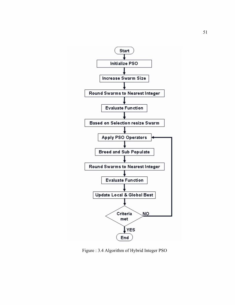
51
Figure : 3.4 Algorithm of Hybrid Integer PSO
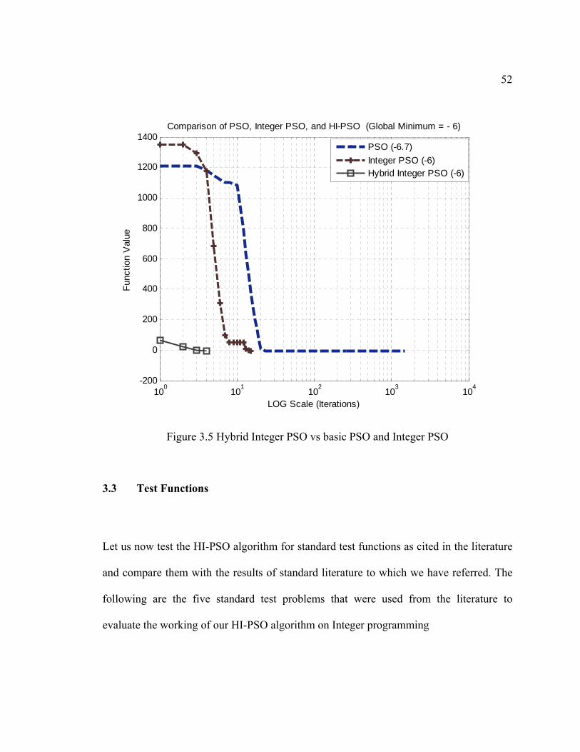
52
100 101 102 103 104-200
0
200
400
600
800
1000
1200
1400
LOG Scale (Iterations)
Func
tion
Val
ueComparison of PSO, Integer PSO, and HI-PSO (Global Minimum = - 6)
PSO (-6.7)Integer PSO (-6)Hybrid Integer PSO (-6)
Figure 3.5 Hybrid Integer PSO vs basic PSO and Integer PSO
3.3 Test Functions
Let us now test the HI-PSO algorithm for standard test functions as cited in the literature
and compare them with the results of standard literature to which we have referred. The
following are the five standard test problems that were used from the literature to
evaluate the working of our HI-PSO algorithm on Integer programming
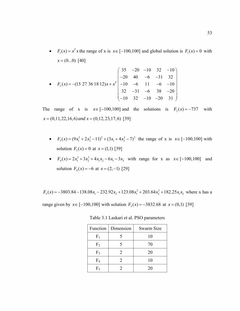
53
• 1( ) TF x x x= the range of x is [ 100,100]x∈ − and global solution is 1( ) 0F x = with
(0...0)x = [40]
• 2
35 20 10 32 1020 40 6 31 32
( ) (15 27 36 18 12) 10 6 11 6 1032 31 6 38 2010 32 10 20 31
TF x x x
− − −⎛ ⎞⎜ ⎟− − −⎜ ⎟⎜ ⎟= − + − − − −⎜ ⎟
− − −⎜ ⎟⎜ ⎟− − −⎝ ⎠
The range of x is [ 100,100]x∈ − and the solutions is 2 ( ) 737F x = − with
(0,11,22,16,6) (0,12,23,17,6)x and x= = [39]
• 2 2 2 2 23 1 2 1 2( ) (9 2 11) (3 4 7)F x x x x x= + − + + − the range of x is [ 100,100]x∈ − with
solution 3( ) 0F x = at (1,1)x = [39]
• 2 24 1 2 1 2 1 2( ) 2 3 4 6 3F x x x x x x x= + + − − with range for x as [ 100,100]x∈ − and
solution 4 ( ) 6F x = − at (2, 1)x = − [29]
2 25 1 2 1 2 1 2( ) 3803.84 138.08 232.92 123.08 203.64 182.25F x x x x x x x= − − − + + + where x has a
range given by [ 100,100]x∈ − with solution 5 ( ) 3832.68F x = − at (0,1)x = [39]
Table 3.1 Laskari et al. PSO parameters
Function Dimension Swarm Size
F1 5 10
F2 5 70
F3 2 20
F4 2 10
F5 2 20
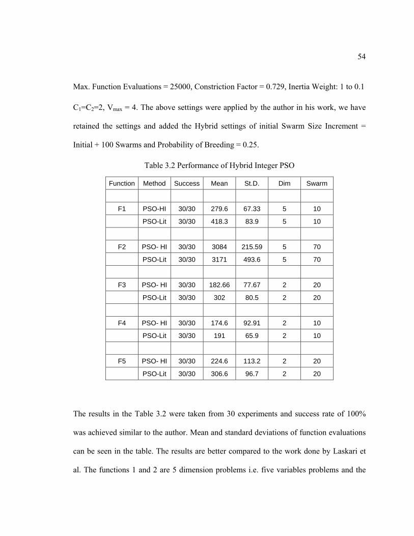
54
Max. Function Evaluations = 25000, Constriction Factor = 0.729, Inertia Weight: 1 to 0.1
C1=C2=2, Vmax = 4. The above settings were applied by the author in his work, we have
retained the settings and added the Hybrid settings of initial Swarm Size Increment =
Initial + 100 Swarms and Probability of Breeding = 0.25.
Table 3.2 Performance of Hybrid Integer PSO
Function Method Success Mean St.D. Dim Swarm
F1 PSO-HI 30/30 279.6 67.33 5 10
PSO-Lit 30/30 418.3 83.9 5 10
F2 PSO- HI 30/30 3084 215.59 5 70
PSO-Lit 30/30 3171 493.6 5 70
F3 PSO- HI 30/30 182.66 77.67 2 20
PSO-Lit 30/30 302 80.5 2 20
F4 PSO- HI 30/30 174.6 92.91 2 10
PSO-Lit 30/30 191 65.9 2 10
F5 PSO- HI 30/30 224.6 113.2 2 20
PSO-Lit 30/30 306.6 96.7 2 20
The results in the Table 3.2 were taken from 30 experiments and success rate of 100%
was achieved similar to the author. Mean and standard deviations of function evaluations
can be seen in the table. The results are better compared to the work done by Laskari et
al. The functions 1 and 2 are 5 dimension problems i.e. five variables problems and the

55
remaining are 2 dimensional problems. Our algorithm stands good to all of these
functions.Hence it is conclusive that an initial large Swarm followed by a breeding it can
do the job better provided it is properly tuned for integer problems.
56
CHAPTER 4
OPTIMIZATION PROBLEM FORMULATION
In industrial plant operations, benefits arise from improved plant performance such as
improved yields of valuable products (or reduced yields of contaminants), reduced energy
consumption, higher processing rates, and longer times between shutdowns. Optimization
can also lead to reduced maintenance costs, less equipment wear, and better utilization of
the process overall. It is extremely helpful to systematically identify the objective,
constraints and degrees of freedom in a process or a plant, leading to such benefits as
improved quality of design, faster and more reliable trouble shooting, and faster decision
making [1].
Predicting benefits must be done with care. Design and operating variables in most
industrial plants are always coupled in some way or another. If the fuel bill for generator
or a distillation column is $3000 per day, a 5 percent savings may justify an energy
conservation project. However, if the process is operated in units then it is incorrect to
just sum up the factors that consume the input and claim a percentage reduction in total
[1].
57
Among the various hierarchies of optimization the design engineers are one. Engineers
engaged in the process design and equipment specification are concerned with the choice
of a process and a nominal operating condition. They are responsible for basic design,
amount of input required, the configuration of the system and assembly of the system so
as to get the operating efficiency to maximum. The simulation tools play a handy role in
helping these engineers achieve the objectives. The other hierarchies may include the
management and plant operations [1].
A significant example of industrial process is Reactive distillation column. The next few
sections will entail about the physical structure process description mathematical
modeling and chemical view point. Section 4.1 is in general about the physical setup of
reactive distillation column. This section also contains the mathematical modeling the
state space design and the optimum design data. Section 4.2 details about the cost
function formulation.
4.1 Reactive Distillation Column
Reactive Distillation is the process of separating reactants, to give products in the
common chamber. It is a non-Linear and complex process to design. The Chemical
industry has already acknowledged its significance due to high gains and its compact
nature [1]. Pre-Installation optimal design of this process is of great concern because it is
58
an installation of one time, but it requires constant supply of materials like fuel and
reactants, out of which fuel is very costly. A saving in the design of an ideal reactive
distillation column (Ideal RDC) [20] without compromising any of the desired features
would indeed be a great profit to the industry. In the chemical process industries,
chemical reaction and purification of the desired products of distillation are usually
carried out sequentially. In many cases, the performance of this classic chemical process
can be significantly improved by integration of reaction and distillation in a single
multifunctional process unit. This integration concept is called ‘reactive distillation’ [2].
Increased process efficiency and reduction of investment and operational costs are the
direct results of this approach. Some of these advantages are realized by using reaction to
improve separation; others are realized by using separation to improve reaction.
RDC is an ideal two-reactant-two-product reactive distillation column proposed by Al-
Arfaj and Luyben [3] and later developed into state space model by Olanrewaju [41]. It
consists of a reactive section in the middle and non-reactive rectifying and stripping
sections at the top and bottom. The column consists of Reactive Trays (NRX) in the
middle, Rectifying Trays (NR) in the Top and Stripping Trays (NS) in the bottom. The
column is numbered from reboiler to condenser. The reaction that takes place in the
reactive zone is exothermic liquid-vapor in nature and is given by
A B C D+ ⇔ + (4.1)
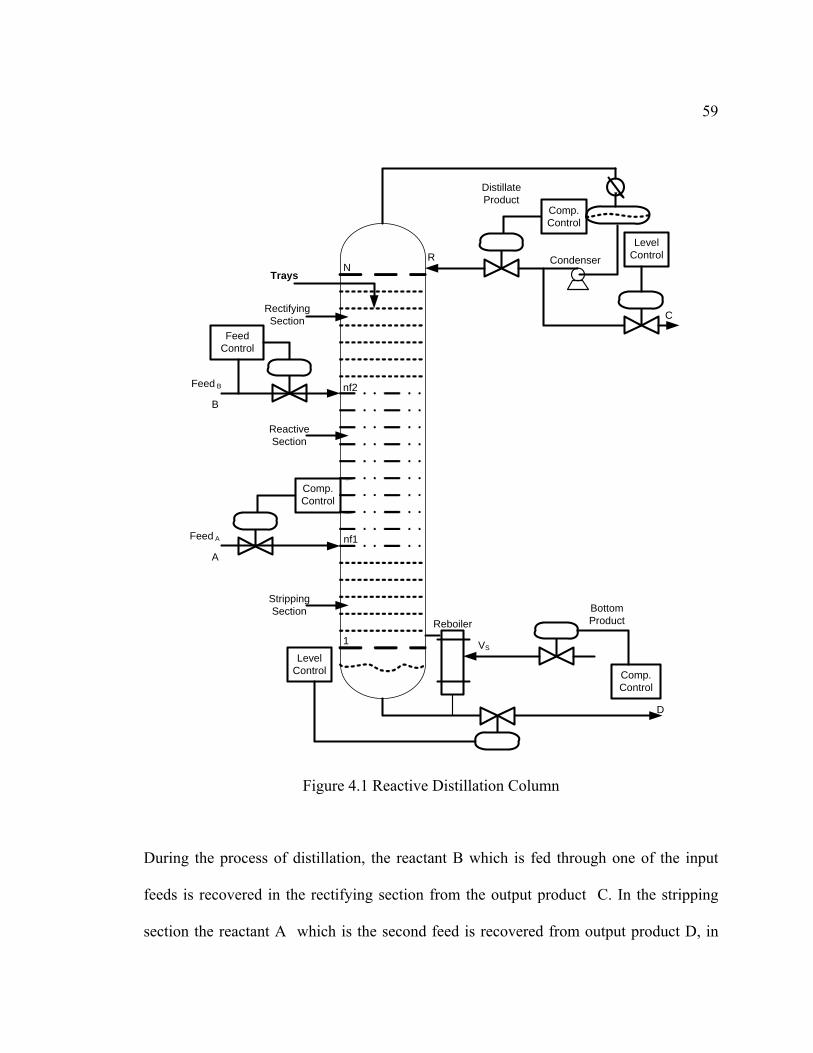
59
Feed B
FeedControl
Comp.Control
nf1
nf2
Feed A
ReactiveSection
RectifyingSection
StrippingSection
N
1
Trays
Comp.Control
RLevel
Control
Distillate Product
LevelControl Comp.
Control
VS
BottomProductReboiler
Condenser
C
D
A
B
Figure 4.1 Reactive Distillation Column
During the process of distillation, the reactant B which is fed through one of the input
feeds is recovered in the rectifying section from the output product C. In the stripping
section the reactant A which is the second feed is recovered from output product D, in
60
the reactive section which comprises the middle section of the reactive distillation
column the products are separated and any undesired reaction between reactants A and B
and products C and D is prevented.
The volatilities of the products and reactants are such that
C A B Dα α α α> > > (4.2)
Where α is the volatility of the Component as can be observed from the above relation C
is the lightest product with highest volatility and D is the heaviest with lightest volatility
along with A and B in between them. This relative volatility ensures that the products A
and B have high concentration in the reactive section, which is typical example of an
Ideal Reactive Distillation column.
The three sections consist of trays that have different Composition Profiles, Vapor
Profile, Liquid Profile and Hold Up. Along the left side two inputs can be seen marked as
FeedA and FeedB. these are the two input streams which feed the reactants A and B, the
reactant A is Lighter compared to B, so when the feeds enter the column, A tries to go up
and since B is heavier than A it tries to settle in the bottom part of the column.
The controllers in the process are termed as dual end composition control structure. The
reflux drum level is controlled by manipulating the distillate flowrate. The purity of both
products is maintained at 95%. In the distillate products, the composition of component C
61
in the distillate is controlled by manipulating the reflux flowrate from the condenser,
while the bottoms composition of component D is controlled by manipulating the vapor
boilup.
4.1.1 Process Modeling
The dynamic model of a Reactive Distillation Column consists of a large number of Non-
Linear Differential equations and demands information about the system such as
composition of trays, vapor, liquid flow rates, liquid holdup in all stages at every instant,
tray hydraulics, energy balances, and vapor liquid equilibrium data. However the system
that is being investigated is an ideal generic reactive distillation with simple vapor-liquid
equilibrium, reaction kinetics and physical properties [41]. The model assumptions are as
follows
1. Ideal Vapor-Liquid Equilibrium
2. Saturated Liquid Feed and Reflux flowrate
3. The energy equations are neglected by assuming constant molar
overflow except in the reactive zone where the vapor flow rate increases
because of the heat of reaction which vaporizes some liquid on each
tray.
4. Constant relative volatilities.
5. Fixed heat of reaction and vaporization and saturated liquid feed and
reflux.
62
The reactive distillation model is based on dynamic mass balance. While the energy
equations are neglected by assuming constant molar overflow except in the reactive zone.
Therefore the nonlinear state space model can be described as follows
1. Reboiler:
( )
BjmBjjBjB yVBxxL
dtxMd
−−= 11 j= 1,2,…, Nc-1 (4.3)
BVLdt
dMm
B −−= 1 (4.4)
Where M is liquid holdup, xij is the liquid mole fraction of component j on tray i, t is the
time in sec, L is the liquid flow rate, B is the bottom flow rate, V is the vapor flow rate, i
is the tray number, j is the component number, B is the bottom tray and Nc is total number
of components which is equal to four.
2. Stripping section, tray i (1< i < Ns+1)
( )
jimjimjiijiiiji yVyVxLxL
dtxMd
,,1,,11 −+−= −++ j= 1, 2,…, Nc-1 (4.5)
iii LL
dtdM
−= +1 (4.6)
Where NS is the number of trays in stripping section.
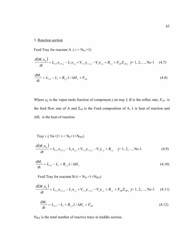
63
3. Reaction section
Feed Tray for reactant A :( i = NS++1)
( )joAoAjijiijiijiijii
iji ZFRyVyVxLxLdt
xMd++−+−= −−++ ,,,11,,11 j= 1, 2,…, Nc-1 (4.7)
oAvjiiii FHRLL
dtdM
+Δ+−= + /,1 λ … …………………(4.8)
Where yij is the vapor mole fraction of component j on tray I, R is the reflux rate, FoA is
the feed flow rate of A and ZoA is the Feed composition of A, λ is heat of reaction and
ΔHv is the heat of reaction
Tray i :( Ns+2< i < NS+1+NRX)
( )
jijiijiijiijiiiji RyVyVxLxL
dtxMd
,,,11,,11 +−+−= −−++ j= 1, 2,…, Nc-1 (4.9)
vjiiii HRLL
dtdM
Δ+−= + /,1 λ (4.10)
Feed Tray for reactant B (i = NS++1+NRX)
( )
joBoBjijiijiijiijiiiji ZFRyVyVxLxL
dtxMd
++−+−= −−++ ,,,11,,11 j= 1, 2,…, Nc-1 (4.11)
oBvjiiii FHRLL
dtdM
+Δ+−= + /,1 λ (4.12)
NRX is the total number of reactive trays in middle section.
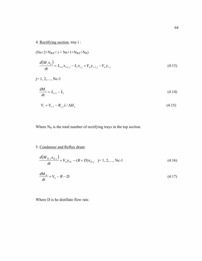
64
4. Rectifying section, tray i :
(Ns+2+NRX< i < Ns+1+NRX+NR)
( )
jinjinjiijiiiji yVyVxLxL
dtxMd
,,1,,11 −+−= −++ (4.13)
j= 1, 2,…, Nc-1
iii LL
dtdM
−= +1 (4.14)
vjiii HRVV Δ−= − /,1 λ (4.15)
Where NR is the total number of rectifying trays in the top section.
5. Condenser and Reflux drum:
( )
jDNrnjDjD xDRyV
dtxMd
,,, )( +−= j= 1, 2,…, Nc-1 (4.16)
DRVdt
dMn
D −−= (4.17)
Where D is he distillate flow rate.
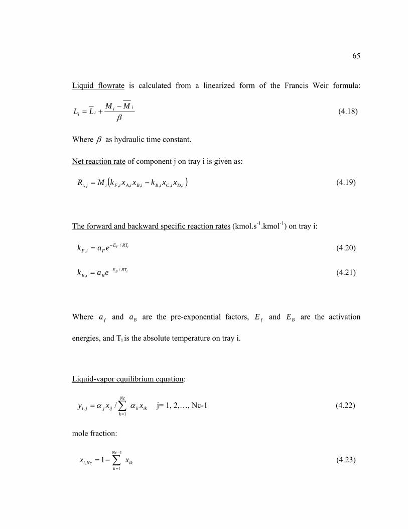
65
Liquid flowrate is calculated from a linearized form of the Francis Weir formula:
βii
iiMM
LL−
+= (4.18)
Where β as hydraulic time constant.
Net reaction rate of component j on tray i is given as:
( )iDiCiBiBiAiFiji xxkxxkMR ,,,,,,, −= (4.19)
The forward and backward specific reaction rates (kmol.s-1.kmol-1) on tray i:
iF RTEFiF eak /
,−= (4.20)
iB RTEBiB eak /
,−= (4.21)
Where fa and Ba are the pre-exponential factors, fE and BE are the activation
energies, and Ti is the absolute temperature on tray i.
Liquid-vapor equilibrium equation:
ikk
Nc
kijjji xxy αα ∑
=
=1
, / j= 1, 2,…, Nc-1 (4.22)
mole fraction:
ik
Nc
kNci xx ∑
−
=
−=1
1, 1 (4.23)
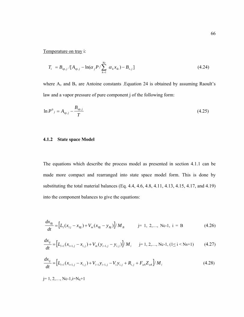
66
Temperature on tray i:
])/ln(/[ ,1
,, jvikk
Nc
kjjvpjvpi BxPABT −−= ∑
=
αα (4.24)
where Av and Bv are Antoine constants .Equation 24 is obtained by assuming Raoult’s
law and a vapor pressure of pure component j of the following form:
TB
AP jvpjvpj
,,
0ln −= (4.25)
4.1.2 State space Model
The equations which describe the process model as presented in section 4.1.1 can be
made more compact and rearranged into state space model form. This is done by
substituting the total material balances (Eq. 4.4, 4.6, 4.8, 4.11, 4.13, 4.15, 4.17, and 4.19)
into the component balances to give the equations:
[ ] BBjBjmBjjBj MyxVxxL
dtdx
/)()( 11 −+−= j= 1, 2,…, Nc-1, i = B (4.26)
[ ] ijijimjijiiij MyyVxxL
dtdx
/)()( ,,1,,11 −+−= −++ j= 1, 2,…, Nc-1, (1< i < Ns+1) (4.27)
[ ] ioAoAjijiijiijijiiij MZFRyVyVxxL
dtdx
/)( ,,,11,,11 ++−+−= −−++ (4.28)
j= 1, 2,…, Nc-1,i=NS+1
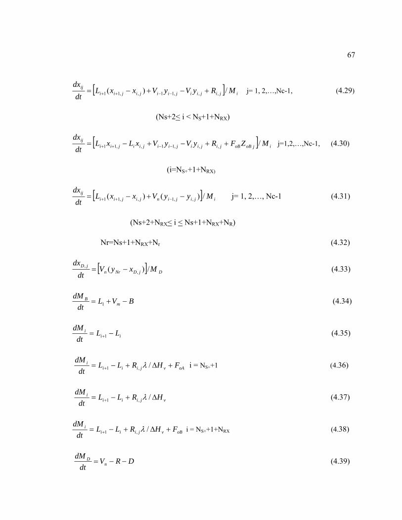
67
[ ] ijijiijiijijiiij MRyVyVxxL
dtdx
/)( ,,,11,,11 +−+−= −−++ j= 1, 2,…,Nc-1, (4.29)
(Ns+2< i < NS+1+NRX)
[ ] ijoBoBjijiijiijiijiiij MZFRyVyVxLxL
dtdx
/,,,11,,11 ++−+−= −−++ j=1,2,…,Nc-1, (4.30)
(i=NS++1+NRX)
[ ] ijijinjijiiij MyyVxxL
dtdx
/)()( ,,1,,11 −+−= −++ j= 1, 2,…, Nc-1 (4.31)
(Ns+2+NRX< i < Ns+1+NRX+NR)
Nr=Ns+1+NRX+Nr (4.32)
[ ] DjDNrnjD MxyV
dtdx
/)( ,, −= (4.33)
BVLdt
dMm
B −+= 1 (4.34)
iii LL
dtdM
−= +1 (4.35)
oAvjiiii FHRLL
dtdM
+Δ+−= + /,1 λ i = NS++1 (4.36)
vjiiii HRLL
dtdM
Δ+−= + /,1 λ (4.37)
oBvjiiii FHRLL
dtdM
+Δ+−= + /,1 λ i = NS++1+NRX (4.38)
DRVdt
dMn
D −−= (4.39)
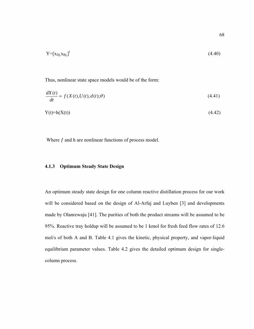
68
Y=[xDj,xBj,]l (4.40)
Thus, nonlinear state space models would be of the form:
));(),(),(()( θtdtUtXfdt
tdX= (4.41)
Y(t)=h(X(t)) (4.42)
Where f and h are nonlinear functions of process model.
4.1.3 Optimum Steady State Design
An optimum steady state design for one column reactive distillation process for our work
will be considered based on the design of Al-Arfaj and Luyben [3] and developments
made by Olanrewaju [41]. The purities of both the product streams will be assumed to be
95%. Reactive tray holdup will be assumed to be 1 kmol for fresh feed flow rates of 12.6
mol/s of both A and B. Table 4.1 gives the kinetic, physical property, and vapor-liquid
equilibrium parameter values. Table 4.2 gives the detailed optimum design for single-
column process.
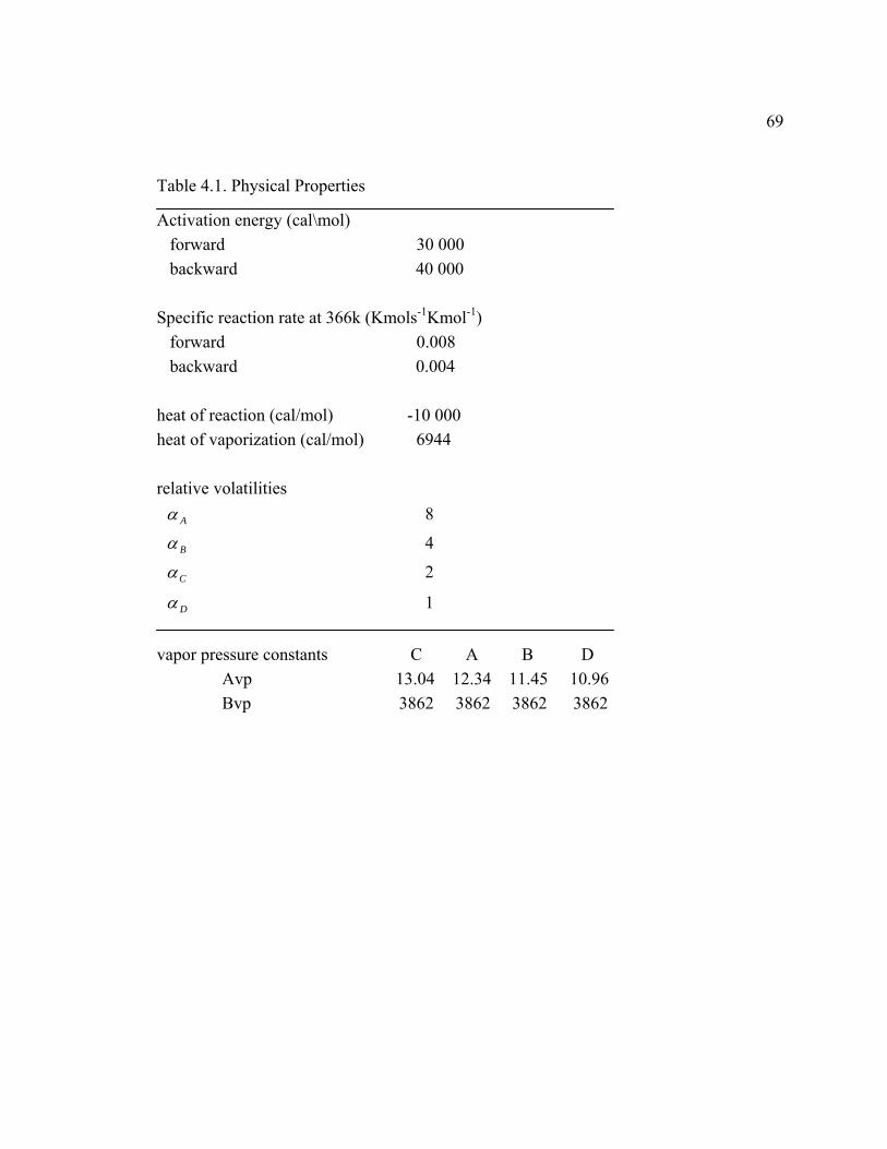
69
Table 4.1. Physical Properties
Activation energy (cal\mol) forward 30 000 backward 40 000 Specific reaction rate at 366k (Kmols-1Kmol-1) forward 0.008 backward 0.004 heat of reaction (cal/mol) -10 000 heat of vaporization (cal/mol) 6944 relative volatilities Aα 8
Bα 4
Cα 2
Dα 1 vapor pressure constants C A B D Avp 13.04 12.34 11.45 10.96 Bvp 3862 3862 3862 3862
70
Table 4.2. Optimum Design for single-column process
Flow rate (mol/s) vapor boil up (mol/s) 28.14 reflux (mol/s) 32.78 distillate (mol/s) 12.6 bottoms (mol/s) 12.6 pressure (bar) 9 tray holdup (Kmol/s) 1.00 Tray numbers Stripping 7 Reactive 6 Rectifying 7 A B C D Composition (mole fraction) distillate 0.04755 0.00246 0.94999 0.00000 bottoms 0.00164 0.04839 0.00000 0.94999
4.2 Cost Function Formulation
The RDC requires a steady temperature inside the column for separation to take place.
This separation is obtained by the method of distillation. The high temperature inside the
column is maintained by the use of reboiler which requires steady supply of fuel. The
amount of fuel consumed per hour to keep the reboiler burning that can maintain a steady
temperature inside the column and produce products of desired purity constitutes the
optimization problem. The ‘cost of fuel consumption’ as an optimization variable is more
significant compared to the ‘cost of pre-installation hardware design’, reason being, the
71
process is one time installation, installation cost compared to the expenditure on fuel over
a long time is small. Hence an optimization of hardware design for low fuel consumption
is very much necessary and significant.
The task of the rectifying section (Top) is to recover reactant B from the product stream
C. In the stripping section (Bottom), the reactant A is stripped from the product stream D.
In the reactive section the products are separated, driving the equilibrium and preventing
any undesired side reactions between the reactants A (or B) with the product C (or D).
Therefore, reactants A and B are intermediate boilers while product C is the lightest and
product D is the heaviest. This ensures that high concentration of the reactants A and B is
maintained in the reactive zone, which is typical for reactive distillation application. The
reactive section contains NRX trays. The rectifying section contains NR trays, and the
stripping section below the reactive section contains NS trays. The column is numbered
from the reboiler to the condenser.
A dual composition control suggested by Al-Arfaj and Luyben [20] is implemented to
obtain the desired manipulated variables. Composition of product C in the distillate is
controlled by manipulating the reflux flowrate, while the vapor boilup is manipulated to
control the bottoms composition of component D. The controllers automatically
manipulated both the reflux flowrate and vapor boilup to the values that correspond to the
desired conversion and purity.
72
The vapor boilup (Vs) in a reactive distillation column is the amount of vapor flowing
from the reboiler into the distillation column. The amount of heat required to vaporize
depends upon the design parameters of the reactive distillation column like number of
trays in each of the three sections, the feed locations and the pressure inside the column.
Hence reducing vapor flow or vapor boilup (Vs) is reducing the amount of fuel
consumed. Nevertheless the quality of components cannot be sacrificed at any price.
Hence a stringent concentration measure of 95% is desired from the system. The vapor
boilup is used to control the bottom composition and the reflux rate is used to control the
Distillate composition. The reflux rate is not optimized. The reason is that the reflux
drum is used for cooling to condense the impurities which are present in vapor form and
send them back to the reactive distillation column for re-processing and re-purification.
The cooling is done by using water jackets and the cost of raw water is negligible
compared to the cost of fuel per day, hence the reflux rate can be neglected.
The fuel consumed by the RDC is equal to the amount of fuel required by the reboiler to
vaporize the liquid and send it back in to the Distillation column.
(1)*2*S BV vss C= (4.43)
Where (1)vss is the vapor holdup of the tray-1(Bottom) at steady state and BC is the
Boiler Constant which is used to control the amount of vapor supplied by the reboiler so
73
as to obtain the desired concentration. The factor BC which is obtained from the reboiler
controller equation checks the concentration of the products and adjusts the reboiler duty.
0.5B B B BC K Er Eri= + +i (4.44)
1.54BK = (4.45)
(0.95 2)0.2BXblagEr −
= (4.46)
Given are 2Xblag Internal Controller Lag and BEri Internal Controller Error. The steady
state vapor boilup is obtained after the Non-Linear equation describing the process is
solved (Eq 4.1 to 4.25). which are dependent up on NS (Stripping Trays), NRX (Reactive
Trays), NR (Rectifying Trays), P (Pressure), NF1 (Feed Location for Input A) and NF2
(Feed Location for Input B). vss is calculated by equation 4.15 recursively.
vjiii HRVV Δ−= − /,1 λ , Where ( )iDiCiBiBiAiFiji xxkxxkMR ,,,,,,, −=
The remainder terms are calculated recursively from the non-Linear Differential
equations from Eq. 4.1 to 4.25
The objective functions can be defined as
I. ( , , )S S RX RV f N N N= for objective 1
II. ( , , , )S S RX RV f N N N P= for objective 2
III. 1 2( , , , , , )S S RX R F FV f N N N P N N= for objective 3
Subject to the condition that concentration of the products is maintained at 95%.
74
CHAPTER 5
SIMULATION AND SETUP
This chapter contains the simulation setup and the results along with discussions.
Section 5.1 gives a brief description about the lab environment for simulation. Section 5.2
describes the optimization setup procedure, this section details about the parameters, the
algorithm, reactive distillation column setup, initial values criterion, range of variables
used and the process run time. Section 5.3 enlists the objective functions section 5.4
illustrates an algorithm that is used to solve the problem. Finally section 5.5 displays he
results and carries the discussions.
5.1 PC Setup
The simulations were carried on over Matlab 6.5 on IBM Compatible PC’s of 512 MB
RAM and Pentium 4 Processors with 2 Giga hertz speed. While the simulation were
being run entire processor was dedicated to Matlab, i.e. 100% Processor time was
dedicated to matlab alone in order to have the maximum efficiency out of the computers.
A cluster of 18 IBM PC’s of identical configurations and a same version of Matlab was
used to check the accuracy of simulations. The cluster was handy when evaluation of
75
objectives was carried by brute force (Exhaustive search) method, thus reducing the
execution time by a factor of 18.
5.2 Optimization Setup
5.2.1 HI-PSO
The variables of the Process were pure integers; HI-PSO was applied to optimize the
process. The algorithm was used as was mentioned in the previous chapter with these
settings.The Hybrid-Integer Particle Swarm Optimization with Vmax operator, Inertia
Weights, Constriction Factor, Neighborhood and Integer Programming along with
breeding and sub-population was used. The simulation was run for a length of 100
iterations and 10 such experiments were carried in order to check the accuracy of the
results. The termination criterion was completion of total iterations i.e. 100.
o Swarm = 20;
o Iterations = 100;
o Cognitive Acceleration (c1) = 2;
o Social Acceleration (c2) = 2;
o Vmax = 4;
o Inertia weights = 1 to 0.1
o Constriction Factor: 0.729
o Neighborhood: Circular
o Initial Swarm: 120
o Breeding Probability : 0.2
o Number of Variables:
76
Objective 1 = 3 (Integer)
Objective 2 = 4 (3 Integer + 1 Real)
Objective 3 = 6 (5 Integer + 1 Real)
5.2.2 Reactive Distillation Column
The Model Proposed by Al-Arfaj and Luyben [20] and Olanrewaju [41] has been used.
Retaining all its originality the model was made variable dependent to accommodate the
change in number of trays (NS ,NRX, NR) and Pressure(P) and the Feed Locations(NF1
NF2). The parameters are given in the chapter 4.
5.2.2.1 Initial Values
As was mentioned earlier, the process is Non-Linear in nature and the order of the
process changes with the change in trays in any of the section. Hence this forms a new
model everytime any of the 3 sections tray quantity is varied. Thus the process requires
that initial values of Liquid profile, composition profile vapor profile and holdup per tray
be provided. This necessity that at every new model there should be initial values present
is fulfilled by extrapolating the values from the base case.
77
The base case had Ns = 7, Nrx = 6 and Nr = 7, so the initial values of
1. Component Composition (22x4)
2. Holdup (22x1)
3. Vapor (22x1)
4. Liquid (22x1)
Profiles consisted of 20 + 2 rows (values), the two extra being the bottom bed and the top
collector which also serve as tray. Ns becomes Ns+1(due to bottom bed) and Nr becomes
Nr+1(due to collector). Ns now becomes 8 Nrx remains same to be 6 and Nr becomes 8.
To find Initial Values of Ns for a Given Model:
1. Find the average of consecutive locations in the Base Ns+1 Values.
2. Insert them in between the two actual locations.
3. Repeat till you reach the end of Ns+1, this gives a total of 2Ns+1 Values,
4. Repeat the above procedure from first step till the length of Ns becomes
greater than or equal to 25
As an Illustration, the 8 values of Ns+1 will generate 7 values after averaging and after
re-insertion in between the source locations the total length becomes 15. upon repeating
the above procedure we will have 15+14 values in Ns. So that becomes 29 which is
greater than 25. The reason we are stopping at greater than 25 is that the maximum range
of any section is between 5 and 25 trays.
78
5. From the stack of these 29 numbers, the selection is made as required
based upon the Model order.
6. For example: in order to have Ns = 10, calculate the Step = 29/10 = 2.9.
7. From the stack of 29 Ns, take step of 2.9 until 29 is reached.
8. since 2.9 is not a perfect integer, take the average of the floor and ceiling
around the number 2.9
9. so the first number will be average of 2nd and 3rd value from the Stack of
29
10. Repeat this loop until the desired vector of initial values is obtained.
The same principle applies to the Nrx and Nr part. From the above procedure all the four
initial value sets can be calculated.
5.2.2.2 Range of Variables
The range of variables used in the simulations is given below:
NS - Stripping Section [5 to 25] NRX - Reactive Section [5 to 25] NR - Rectifying Section [5 to 25] P – Column Pressure [5 to 15]
NF1 - Stripping Section [NS - 5 to 2RXN ]
NF2 - Stripping Section [ 12RXN
+ to NS + NRX + 5]
For all the three objectives this range was maintained.
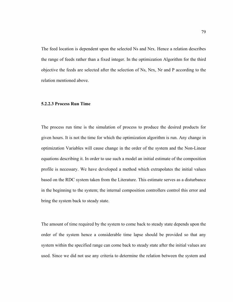
79
The feed location is dependent upon the selected Ns and Nrx. Hence a relation describes
the range of feeds rather than a fixed integer. In the optimization Algorithm for the third
objective the feeds are selected after the selection of Ns, Nrx, Nr and P according to the
relation mentioned above.
5.2.2.3 Process Run Time
The process run time is the simulation of process to produce the desired products for
given hours. It is not the time for which the optimization algorithm is run. Any change in
optimization Variables will cause change in the order of the system and the Non-Linear
equations describing it. In order to use such a model an initial estimate of the composition
profile is necessary. We have developed a method which extrapolates the initial values
based on the RDC system taken from the Literature. This estimate serves as a disturbance
in the beginning to the system; the internal composition controllers control this error and
bring the system back to steady state.
The amount of time required by the system to come back to steady state depends upon the
order of the system hence a considerable time lapse should be provided so that any
system within the specified range can come back to steady state after the initial values are
used. Since we did not use any criteria to determine the relation between the system and
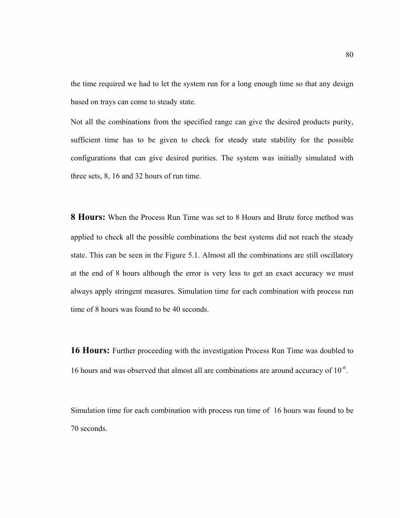
80
the time required we had to let the system run for a long enough time so that any design
based on trays can come to steady state.
Not all the combinations from the specified range can give the desired products purity,
sufficient time has to be given to check for steady state stability for the possible
configurations that can give desired purities. The system was initially simulated with
three sets, 8, 16 and 32 hours of run time.
8 Hours: When the Process Run Time was set to 8 Hours and Brute force method was
applied to check all the possible combinations the best systems did not reach the steady
state. This can be seen in the Figure 5.1. Almost all the combinations are still oscillatory
at the end of 8 hours although the error is very less to get an exact accuracy we must
always apply stringent measures. Simulation time for each combination with process run
time of 8 hours was found to be 40 seconds.
16 Hours: Further proceeding with the investigation Process Run Time was doubled to
16 hours and was observed that almost all are combinations are around accuracy of 10-6.
Simulation time for each combination with process run time of 16 hours was found to be
70 seconds.
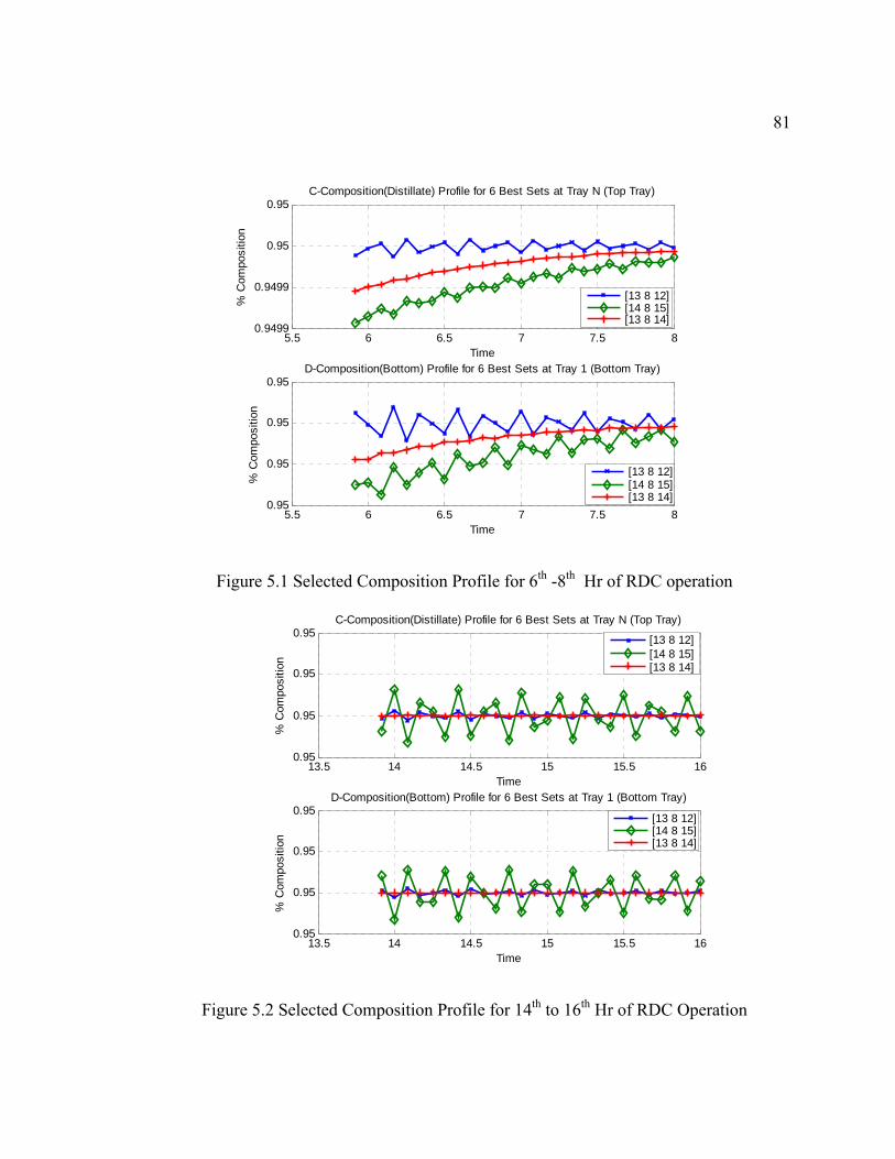
81
5.5 6 6.5 7 7.5 80.9499
0.9499
0.95
0.95
Time
% C
ompo
sitio
n
C-Composition(Distillate) Profile for 6 Best Sets at Tray N (Top Tray)
[13 8 12][14 8 15][13 8 14]
5.5 6 6.5 7 7.5 80.95
0.95
0.95
0.95
Time
% C
ompo
sitio
n
D-Composition(Bottom) Profile for 6 Best Sets at Tray 1 (Bottom Tray)
[13 8 12][14 8 15][13 8 14]
Figure 5.1 Selected Composition Profile for 6th -8th Hr of RDC operation
13.5 14 14.5 15 15.5 160.95
0.95
0.95
0.95
Time
% C
ompo
sitio
n
C-Composition(Distillate) Profile for 6 Best Sets at Tray N (Top Tray)
[13 8 12][14 8 15][13 8 14]
13.5 14 14.5 15 15.5 160.95
0.95
0.95
0.95
Time
% C
ompo
sitio
n
D-Composition(Bottom) Profile for 6 Best Sets at Tray 1 (Bottom Tray)
[13 8 12][14 8 15][13 8 14]
Figure 5.2 Selected Composition Profile for 14th to 16th Hr of RDC Operation
82
32 Hours: A third option was chosen to quadruple the initial time, i.e. to make the
Process Run Time to 32 hours, it was seen that without doubt all the combinations were
achieving steady state to an accuracy of 10-12.
29.5 30 30.5 31 31.5 320.95
0.95
0.95
0.95
Time
% C
ompo
sitio
n
C-Composition(Distillate) Profile for 6 Best Sets at Tray N (Top Tray)
[13 8 12][14 8 15][13 8 14]
29.5 30 30.5 31 31.5 320.95
0.95
0.95
0.95
Time
% C
ompo
sitio
n
D-Composition(Bottom) Profile for 6 Best Sets at Tray 1 (Bottom Tray)
[13 8 12][14 8 15][13 8 14]
Figure 5.3 Selected Composition Profile for 30th -32nd Hr of RDC operation
Simulation time for each combination with process run time of 32 hours was found to be
105 seconds.
A minute and half per combination would mean 30 minutes per iteration based on a
Swarm of size 20, and 100 iterations would mean a time of 50 hours. That is very huge
time to dedicate. Although this computational time depends upon the type of CPU and
83
the RAM. In the best interest it was decided to use a Process Run Time of 16 hours
without compromising the accuracy.
5.3 Objective Function
The cost function as explained in chapter 4.2 can be summarized as follows:
Objective 1: 1 1( , , ) (95 ) (95 )S S RX R B DV f N N N k C k C= + − + −
With Pressure = 9 bar, NF1 = NS + 2 and NF2 = NS + NRX + 1
Objective 2: 1 1( , , , ) (95 ) (95 )S S RX R B DV f N N N P k C k C= + − + −
with Pressure = 9 bar,
Objective 3: 1 2 1 1( , , , , , ) (95 ) (95 )S S RX R F F B DV f N N N P N N k C k C= + − + −
Where k1 is penalty factor with a very high value and CB and CD are concentrations of
Bottom and Distillate products whose desired value is 95%. These objective functions are
referred to as equality constraints wherein if a condition is not satisfied a high penalty is
applied.
84
5.4 Algorithm
The algorithm, generalized for third objective, is started by initializing a large swarm
consisting of the Stripping, Reactive, Rectifying Trays and Pressure. From the randomly
generated swarm the location of feeds are generated using the stripping and reactive
Trays the two swarms are merged to form one single swarm the rounding operation is
performed on all but the pressure variable, initial values are determined for the RDC
based on the swarm and the process is operated for 16 hours using each combination, the
best among the swarm are selected after the cost function is evaluated to resize the swarm
back to its original size. The velocity and positions of particles are updated using the HI-
PSO and the algorithm is re-iterated until; the termination criterion is met.
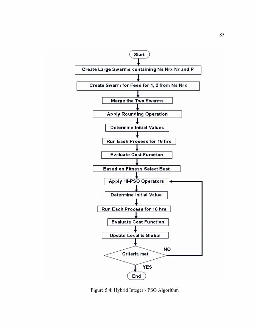
85
Figure 5.4: Hybrid Integer - PSO Algorithm
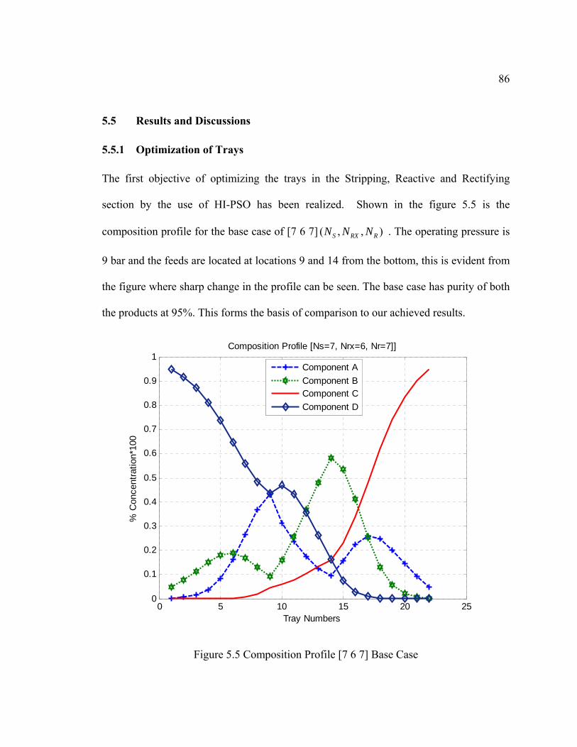
86
5.5 Results and Discussions
5.5.1 Optimization of Trays
The first objective of optimizing the trays in the Stripping, Reactive and Rectifying
section by the use of HI-PSO has been realized. Shown in the figure 5.5 is the
composition profile for the base case of [7 6 7] ( , , )S RX RN N N . The operating pressure is
9 bar and the feeds are located at locations 9 and 14 from the bottom, this is evident from
the figure where sharp change in the profile can be seen. The base case has purity of both
the products at 95%. This forms the basis of comparison to our achieved results.
0 5 10 15 20 250
0.1
0.2
0.3
0.4
0.5
0.6
0.7
0.8
0.9
1
Tray Numbers
% C
once
ntra
tion*
100
Composition Profile [Ns=7, Nrx=6, Nr=7]]
Component AComponent BComponent CComponent D
Figure 5.5 Composition Profile [7 6 7] Base Case
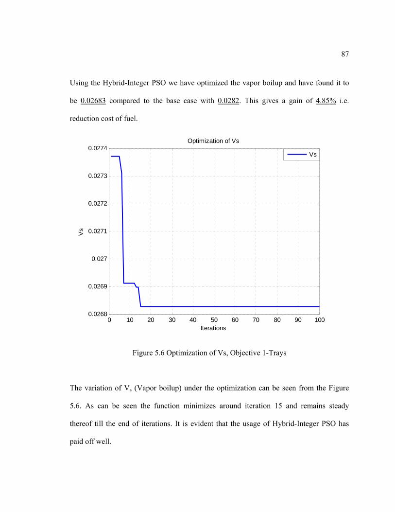
87
Using the Hybrid-Integer PSO we have optimized the vapor boilup and have found it to
be 0.02683 compared to the base case with 0.0282. This gives a gain of 4.85% i.e.
reduction cost of fuel.
0 10 20 30 40 50 60 70 80 90 1000.0268
0.0269
0.027
0.0271
0.0272
0.0273
0.0274
Iterations
Vs
Optimization of Vs
Vs
Figure 5.6 Optimization of Vs, Objective 1-Trays
The variation of Vs (Vapor boilup) under the optimization can be seen from the Figure
5.6. As can be seen the function minimizes around iteration 15 and remains steady
thereof till the end of iterations. It is evident that the usage of Hybrid-Integer PSO has
paid off well.
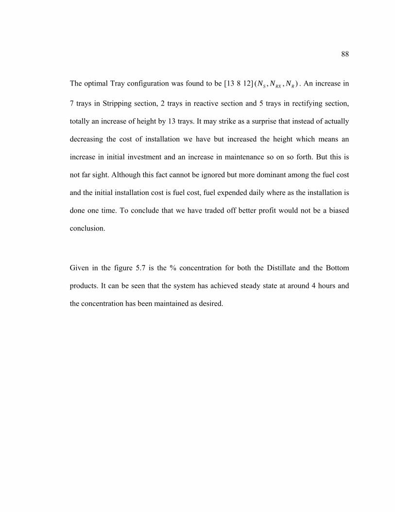
88
The optimal Tray configuration was found to be [13 8 12] ( , , )S RX RN N N . An increase in
7 trays in Stripping section, 2 trays in reactive section and 5 trays in rectifying section,
totally an increase of height by 13 trays. It may strike as a surprise that instead of actually
decreasing the cost of installation we have but increased the height which means an
increase in initial investment and an increase in maintenance so on so forth. But this is
not far sight. Although this fact cannot be ignored but more dominant among the fuel cost
and the initial installation cost is fuel cost, fuel expended daily where as the installation is
done one time. To conclude that we have traded off better profit would not be a biased
conclusion.
Given in the figure 5.7 is the % concentration for both the Distillate and the Bottom
products. It can be seen that the system has achieved steady state at around 4 hours and
the concentration has been maintained as desired.
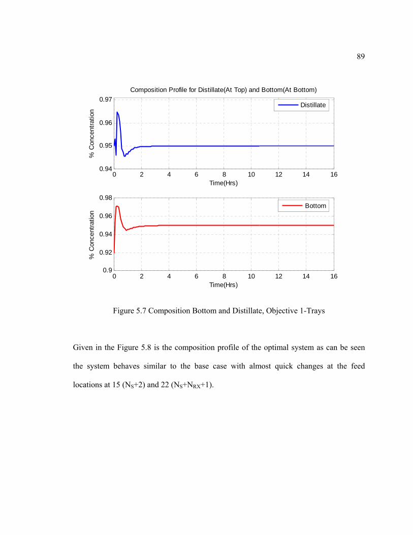
89
0 2 4 6 8 10 12 14 160.94
0.95
0.96
0.97
Time(Hrs)
% C
once
ntra
tion
Composition Profile for Distillate(At Top) and Bottom(At Bottom)
Distillate
0 2 4 6 8 10 12 14 160.9
0.92
0.94
0.96
0.98
Time(Hrs)
% C
once
ntra
tion
Bottom
Figure 5.7 Composition Bottom and Distillate, Objective 1-Trays
Given in the Figure 5.8 is the composition profile of the optimal system as can be seen
the system behaves similar to the base case with almost quick changes at the feed
locations at 15 (NS+2) and 22 (NS+NRX+1).
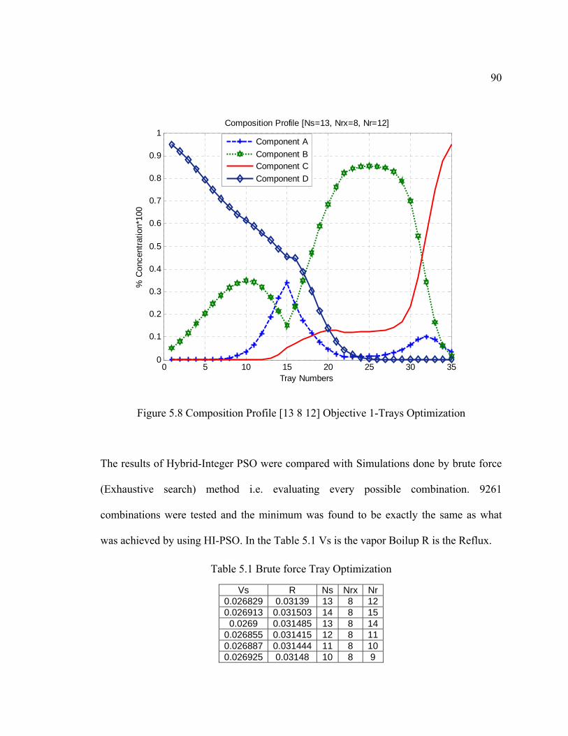
90
0 5 10 15 20 25 30 350
0.1
0.2
0.3
0.4
0.5
0.6
0.7
0.8
0.9
1
Tray Numbers
% C
once
ntra
tion*
100
Composition Profile [Ns=13, Nrx=8, Nr=12]
Component AComponent BComponent CComponent D
Figure 5.8 Composition Profile [13 8 12] Objective 1-Trays Optimization
The results of Hybrid-Integer PSO were compared with Simulations done by brute force
(Exhaustive search) method i.e. evaluating every possible combination. 9261
combinations were tested and the minimum was found to be exactly the same as what
was achieved by using HI-PSO. In the Table 5.1 Vs is the vapor Boilup R is the Reflux.
Table 5.1 Brute force Tray Optimization
Vs R Ns Nrx Nr0.026829 0.03139 13 8 120.026913 0.031503 14 8 150.0269 0.031485 13 8 14
0.026855 0.031415 12 8 110.026887 0.031444 11 8 100.026925 0.03148 10 8 9
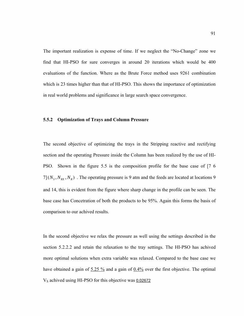
91
The important realization is expense of time. If we neglect the “No-Change” zone we
find that HI-PSO for sure converges in around 20 iterations which would be 400
evaluations of the function. Where as the Brute Force method uses 9261 combination
which is 23 times higher than that of HI-PSO. This shows the importance of optimization
in real world problems and significance in large search space convergence.
5.5.2 Optimization of Trays and Column Pressure
The second objective of optimizing the trays in the Stripping reactive and rectifying
section and the operating Pressure inside the Column has been realized by the use of HI-
PSO. Shown in the figure 5.5 is the composition profile for the base case of [7 6
7] ( , , )S RX RN N N . The operating pressure is 9 atm and the feeds are located at locations 9
and 14, this is evident from the figure where sharp change in the profile can be seen. The
base case has Concetration of both the products to be 95%. Again this forms the basis of
comparison to our achived results.
In the second objective we relax the pressure as well using the settings described in the
section 5.2.2.2 and retain the relaxation to the tray settings. The HI-PSO has achived
more optimal solutions when extra variable was relaxed. Compared to the base case we
have obtained a gain of 5.25 % and a gain of 0.4% over the first objective. The optimal
VS achived using HI-PSO for this objective was 0.02672
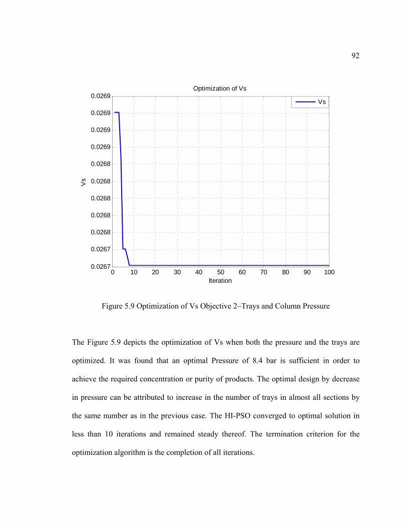
92
0 10 20 30 40 50 60 70 80 90 1000.0267
0.0267
0.0268
0.0268
0.0268
0.0268
0.0268
0.0269
0.0269
0.0269
0.0269
Iteration
Vs
Optimization of Vs
Vs
Figure 5.9 Optimization of Vs Objective 2–Trays and Column Pressure
The Figure 5.9 depicts the optimization of Vs when both the pressure and the trays are
optimized. It was found that an optimal Pressure of 8.4 bar is sufficient in order to
achieve the required concentration or purity of products. The optimal design by decrease
in pressure can be attributed to increase in the number of trays in almost all sections by
the same number as in the previous case. The HI-PSO converged to optimal solution in
less than 10 iterations and remained steady thereof. The termination criterion for the
optimization algorithm is the completion of all iterations.
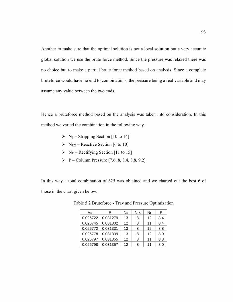
93
Another to make sure that the optimal solution is not a local solution but a very accurate
global solution we use the brute force method. Since the pressure was relaxed there was
no choice but to make a partial brute force method based on analysis. Since a complete
bruteforce would have no end to combinations, the pressure being a real variable and may
assume any value between the two ends.
Hence a bruteforce method based on the analysis was taken into consideration. In this
method we varied the combination in the following way.
NS – Stripping Section [10 to 14]
NRX – Reactive Section [6 to 10]
NR – Rectifying Section [11 to 15]
P – Column Pressure [7.6, 8, 8.4, 8.8, 9.2]
In this way a total combination of 625 was obtained and we charted out the best 6 of
those in the chart given below.
Table 5.2 Bruteforce - Tray and Pressure Optimization
Vs R Ns Nrx Nr P 0.026722 0.031279 13 8 12 8.4 0.026745 0.031302 12 8 11 8.4 0.026772 0.031331 13 8 12 8.8 0.026778 0.031339 13 8 12 8.0 0.026797 0.031355 12 8 11 8.8 0.026798 0.031357 12 8 11 8.0
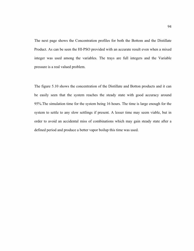
94
The next page shows the Concentration profiles for both the Bottom and the Distillate
Product. As can be seen the HI-PSO provided with an accurate result even when a mixed
integer was used among the variables. The trays are full integers and the Variable
pressure is a real valued problem.
The figure 5.10 shows the concentration of the Distillate and Botton products and it can
be easily seen that the system reaches the steady state with good accuracy around
95%.The simulation time for the system being 16 hours. The time is large enough for the
system to settle to any slow settlings if present. A lesser time may seem viable, but in
order to avoid an accidental miss of combinations which may gain steady state after a
defined period and produce a better vapor boilup this time was used.
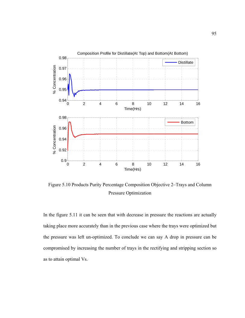
95
0 2 4 6 8 10 12 14 160.94
0.95
0.96
0.97
0.98
Time(Hrs)
% C
once
ntra
tion
Composition Profile for Distillate(At Top) and Bottom(At Bottom)
Distillate
0 2 4 6 8 10 12 14 160.9
0.92
0.94
0.96
0.98
Time(Hrs)
% C
once
ntra
tion
Bottom
Figure 5.10 Products Purity Percentage Composition Objective 2–Trays and Column
Pressure Optimization
In the figure 5.11 it can be seen that with decrease in pressure the reactions are actually
taking place more accurately than in the previous case where the trays were optimized but
the pressure was left un-optimized. To conclude we can say A drop in pressure can be
compromised by increasing the number of trays in the rectifying and stripping section so
as to attain optimal Vs.
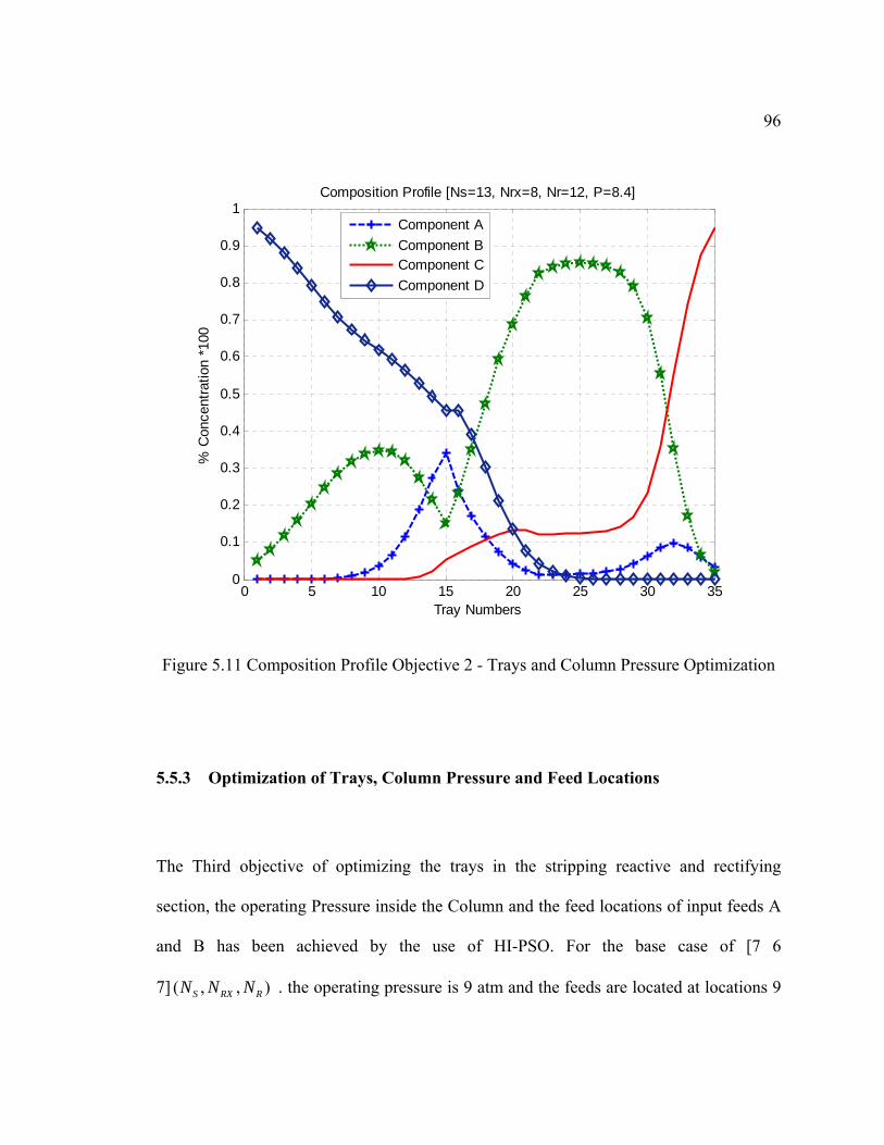
96
0 5 10 15 20 25 30 350
0.1
0.2
0.3
0.4
0.5
0.6
0.7
0.8
0.9
1
Tray Numbers
% C
once
ntra
tion
*100
Composition Profile [Ns=13, Nrx=8, Nr=12, P=8.4]
Component AComponent BComponent CComponent D
Figure 5.11 Composition Profile Objective 2 - Trays and Column Pressure Optimization
5.5.3 Optimization of Trays, Column Pressure and Feed Locations
The Third objective of optimizing the trays in the stripping reactive and rectifying
section, the operating Pressure inside the Column and the feed locations of input feeds A
and B has been achieved by the use of HI-PSO. For the base case of [7 6
7] ( , , )S RX RN N N . the operating pressure is 9 atm and the feeds are located at locations 9
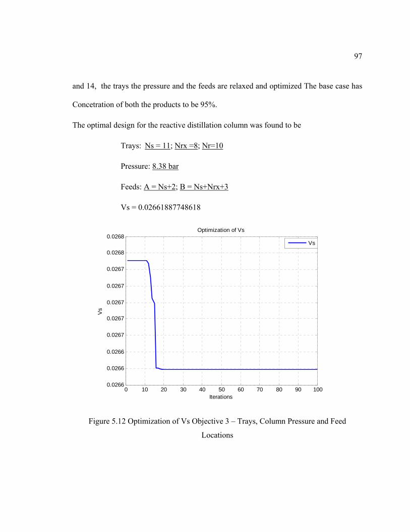
97
and 14, the trays the pressure and the feeds are relaxed and optimized The base case has
Concetration of both the products to be 95%.
The optimal design for the reactive distillation column was found to be
Trays: Ns = 11; Nrx =8; Nr=10
Pressure: 8.38 bar
Feeds: A = Ns+2; B = Ns+Nrx+3
Vs = 0.02661887748618
0 10 20 30 40 50 60 70 80 90 1000.0266
0.0266
0.0266
0.0267
0.0267
0.0267
0.0267
0.0267
0.0268
0.0268
Iterations
Vs
Optimization of Vs
Vs
Figure 5.12 Optimization of Vs Objective 3 – Trays, Column Pressure and Feed
Locations
98
HI-PSO has optimized the design of reactive distillation column and has saved 6% of cost
in fuel consumption for the process compared to the base case of ideal RDC. Although
the algorithm has taken a little longer than the previous two cases but still it is a best bet.
This objective had 5 integer variables and one real variable. The algorithm converged to
optimal solution in less than 20 iterations as can be seen in figure 5.12. This is a fast
solution taking into account the time it would have taken if bruteforce method is applied
to this problem. Based on the previous results we conclude that the HI-PSO converged
onto better solution with faster pace.
Over all the optimal system height was increased by 9 trays, the pressure was dropped by
around 0.62 bar and the feed location for feed 2 needed to be shifted up towards the
‘TOP’ in order to achieve the optimal Vs.
The composition profiles show that the system achieved steady state before 3 hours and
remained steady there after. The concentration profiles show the characteristics of the
system under the new design.
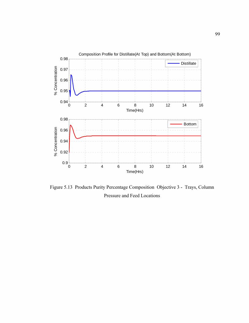
99
0 2 4 6 8 10 12 14 160.94
0.95
0.96
0.97
0.98
Time(Hrs)
% C
once
ntra
tion
Composition Profile for Distillate(At Top) and Bottom(At Bottom)
Distillate
0 2 4 6 8 10 12 14 160.9
0.92
0.94
0.96
0.98
Time(Hrs)
% C
once
ntra
tion
Bottom
Figure 5.13 Products Purity Percentage Composition Objective 3 - Trays, Column
Pressure and Feed Locations
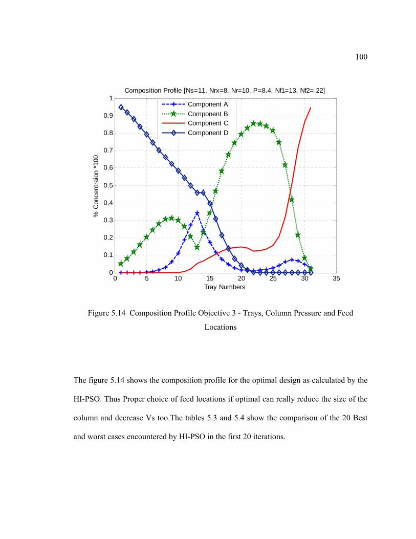
100
0 5 10 15 20 25 30 350
0.1
0.2
0.3
0.4
0.5
0.6
0.7
0.8
0.9
1
Tray Numbers
% C
once
ntra
ion
*100
Composition Profile [Ns=11, Nrx=8, Nr=10, P=8.4, Nf1=13, Nf2= 22]
Component AComponent BComponent CComponent D
Figure 5.14 Composition Profile Objective 3 - Trays, Column Pressure and Feed
Locations
The figure 5.14 shows the composition profile for the optimal design as calculated by the
HI-PSO. Thus Proper choice of feed locations if optimal can really reduce the size of the
column and decrease Vs too.The tables 5.3 and 5.4 show the comparison of the 20 Best
and worst cases encountered by HI-PSO in the first 20 iterations.
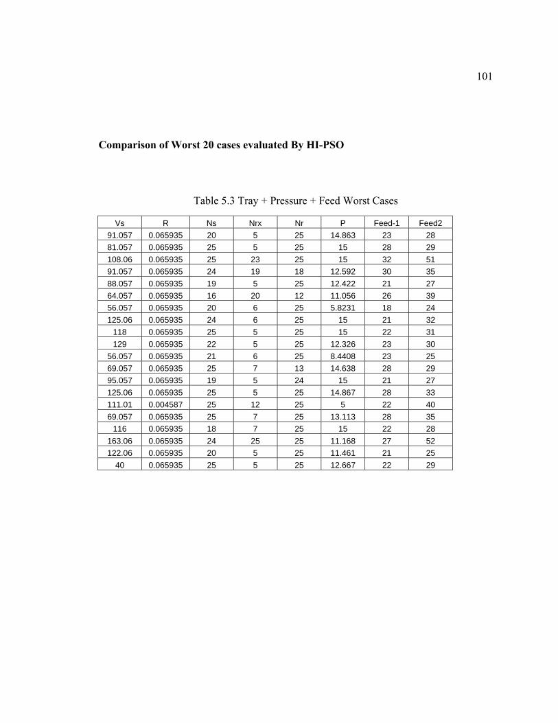
101
Comparison of Worst 20 cases evaluated By HI-PSO
Table 5.3 Tray + Pressure + Feed Worst Cases
Vs R Ns Nrx Nr P Feed-1 Feed2 91.057 0.065935 20 5 25 14.863 23 28 81.057 0.065935 25 5 25 15 28 29 108.06 0.065935 25 23 25 15 32 51 91.057 0.065935 24 19 18 12.592 30 35 88.057 0.065935 19 5 25 12.422 21 27 64.057 0.065935 16 20 12 11.056 26 39 56.057 0.065935 20 6 25 5.8231 18 24 125.06 0.065935 24 6 25 15 21 32
118 0.065935 25 5 25 15 22 31 129 0.065935 22 5 25 12.326 23 30
56.057 0.065935 21 6 25 8.4408 23 25 69.057 0.065935 25 7 13 14.638 28 29 95.057 0.065935 19 5 24 15 21 27 125.06 0.065935 25 5 25 14.867 28 33 111.01 0.004587 25 12 25 5 22 40 69.057 0.065935 25 7 25 13.113 28 35
116 0.065935 18 7 25 15 22 28 163.06 0.065935 24 25 25 11.168 27 52 122.06 0.065935 20 5 25 11.461 21 25
40 0.065935 25 5 25 12.667 22 29
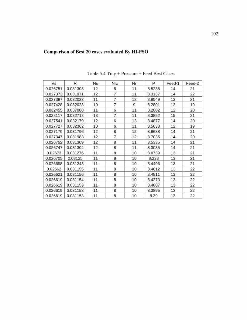
102
Comparison of Best 20 cases evaluated By HI-PSO
Table 5.4 Tray + Pressure + Feed Best Cases
Vs R Ns Nrx Nr P Feed-1 Feed-2 0.026751 0.031308 12 8 11 8.5235 14 21 0.027373 0.031971 12 7 11 8.3137 14 22 0.027397 0.032023 11 7 12 8.8549 13 21 0.027428 0.032023 10 7 9 8.2801 12 19 0.032455 0.037088 11 6 11 8.2002 12 20 0.028117 0.032713 13 7 11 8.3852 15 21 0.027541 0.032179 12 6 13 8.4877 14 20 0.027727 0.032362 10 6 11 8.5638 12 19 0.027179 0.031796 12 8 12 8.6688 14 21 0.027347 0.031983 12 7 12 8.7035 14 20 0.026752 0.031309 12 8 11 8.5335 14 21 0.026747 0.031304 12 8 11 8.3035 14 21 0.02673 0.031276 11 8 10 8.0739 13 21 0.026705 0.03125 11 8 10 8.233 13 21 0.026698 0.031243 11 8 10 8.4496 13 21 0.02662 0.031155 11 8 10 8.4612 13 22 0.026621 0.031156 11 8 10 8.4811 13 22 0.026619 0.031154 11 8 10 8.4273 13 22 0.026619 0.031153 11 8 10 8.4007 13 22 0.026619 0.031153 11 8 10 8.3895 13 22 0.026619 0.031153 11 8 10 8.39 13 22
103
CHAPTER 6
CONCLUSIONS AND RECOMMENDATIONS
6.1 Conclusions
Integer PSO can handle integer problems very well, but the main problem encountered in
Integer PSO is that the convergence rate is not very fast although it’s good. In systems
like RDC which is highly non-linear, takes a lot of time to simulate. Large number of
iterations would mean large amount of time. Hybrid PSO with breeding and sub-
population has the ability to enhance the convergence rate very fast and obtain the global
minima without getting stuck in local minima. A hybrid-Integer PSO resulting from
Large Initial Swarm, Integer PSO and Hybrid PSO thus provides faster convergence in
small number of iterations to problems like that of RDC. HI-PSO can be applied to a
wide variety of problems ranging from simple mathematical to complex and hard
industrial problems which are integer based. The development of Hybrid Integer PSO has
added to the results and has proved to be more powerful than the standard integer PSO.
An ideal Reactive distillation column can be optimized by finding the optimal number of
trays in the stripping, reactive and rectifying section along with the pressure in the
column and proper feed locations.
104
An increase in trays for an optimal design provided the fuel factor Vs is low is not a bad
compromise to make. The height of the tower or the installation of trays being a one time
installation may look like a gross input. But the savings made on fuel of about 6% per
hour does really prove to be significant.
A drop in pressure can be compromised by increasing the number of trays in the
rectifying and stripping section so as to attain optimal Vs.
Proper choice of feed locations if optimal can really reduce the size of the column and
decrease Vs too.
6.2 Recommendations for Future Work
• HI-PSO can be used in parallel environment where every particle can be evaluated
separately.
• HI-PSO may be coded for distributed environment where there exists a Master-
Slave network.
• With in the search space the distributed PSO can greatly effect the time of
simulation, hence a cluster of PC’s can be used to serve the purpose of distributed
PSO.

105
• A generic algorithm can be designed based on the principle of chemical
engineering to find the initial values with using the method of extrapolation.
• Effect of optimizing the Tray + Feed and Feed + Pressure can also be investigated
although may sound simple, but this may give some more insight on the behavior
of RDC.
• Other variables like the molar holdup, height of the tower can be introduced as
optimization parameters.
106
REFERENCES
1. Edgar, Himmelblau and Lasdon “Optimization of Chemical Processes” McGraw-Hill
2001
2. K. Sundmacher and A. Kienle, "Reactive distillation: status and future directions."
Weinheim: WILEY-VCH, 2003
3. Al-Arfaj, M.A & Luyben, W. L. “Effect of Number of Fractionating Trays on
Reactive Distillation Performance,” AIChE Journal; v46; 2417-2425; 2000
4. Ciric, A. R., & Gu, D. (1994). Synthesis of nonequilibrium reactive distillation
processes by MINLP optimization. AIChE Journal, 40(9), 1479.
5. Z. Michalewicz, and D. B. Fogel, “How to Solve It: Modern Heuristics”, Springer-
Verlag Berlin Heidelberg New York (2002)
6. J. H. Holland, “Adaptation in Natural and Arti_cial Systems”, University of Michigan
Press, Ann Arbor, 1929.
7. T. Back, D. B. Fogel, and Z. Michalewicz, “Handbook of Evolutionary
Computation”, Oxford University Press, (1997).
8. S. Hackwood, and G. Beni, “Self-Organization of Sensors for Swarm Intelligence”, In
Proceedings IEEE 1992 International Conference on Robotics and Automation, Los
Alamitos, CA: IEEE Computer Society Press, (1992):819-829.
9. E. Bonabeau, M. Dorigo and G. Theraulaz, “Swarm Intelligence: “From Natural to
Arti_cial Systems”, Oxford University Press Inc., ISBN 0-19-513158-4 (cloth); ISBN
0-19-513159-2 (pbk.), (1999): 1-22.
107
10. M. F. Cardoso, R. L. Salcedo, S. Feyo de Azevedo, D. Barbosa “Optimization of
reactive distillation processes with simulated annealing” Chemical Engineering
Science 55 (2000) 5059-5078
11. J. Kennedy, and R. C. Eberhart, “Swarm Intelligence”, ISBN 1-55860-595-9,
Academic Press (2001).
12. J. Kennedy, and R. C. Eberhart, “Particle swarm optimization”,Proceedings of the
1995 IEEE International Conference on Neural Networks,vol. 4, IEEE Press, (1995):
1942-1948.
13. P. J. Angeline, “Evolutionary Optimization versus Particle Swarm Optimization:
Philosophy and Performance Differences”, Evolutionary Programming VII, Lecture
Notes in Computer Science 1447, Springer, (1998):601-610.
14. J. Kennedy, “Small Worlds and Mega-Minds: Effects of Neighborhood Topology on
Particle Swarm Performance”, Proceedings of the 1999 Congress of Evolutionary
Computation, vol. 3, IEEE Press, (1999): 1931-1938.
15. M. Clerc, and J. Kennedy, “The Particle Swarm - Explosion, Stability, and
Convergence in a Multidimensional Complex Space”, IEEE Transactions on
Evolutionary Computation, Vol. 6, No. 1, February, (2002): 58-73.
16. M. Løvbjerg, T. K. Rasmussen, and T. Krink, “Hybrid Particle Swarm Optimiser with
Breeding and Subpopulations”, Proceedings of the third Genetic and Evolutionary
Computation Conference (GECCO-2001).
108
17. A. Carlisle, and G. Dozier, “An off-the-shelf PSO”, Proceedings of the workshop on
particle swarm optimization, Purdue school of engineering and technology,
Indianapolis, IN, (2001).
18. Y. Shi and R. C. Eberhart, “Parameter Selection in Particle Swarm Optimization”,
Evolutionary Programming VII, Springer, Lecture Notes in Computer Science 1447,
(1998): 591-600.
19. Y. Shi, and R. C. Eberhart, “Empirical Study of Particle Swarm Optimization”,
Proceedings of the 1999 Congress of Evolutionary Computation, vol. 3, IEEE Press,
(1999): 1945-1950.
20. M. A. Al-Arfaj and W. L. Luyben, "Comparison of alternative control structures for
an ideal two-product reactive distillation column," Ind. Eng. Chem. Res., vol. 39, pp.
3298-3307, 2000.
21. Parsopoulos, K.E., Vrahatis, M.N. “On the computation of all global minimizers
through particle swarm optimization”. IEEE Trans. Evol. Comp. 8 (2004) 211–224
22. K. Sundmacher and A. Kienle, "Reactive distillation: status and future directions."
Weinheim: WILLEY-VCH, 2003.
23. R. Taylor and R. Krishna, "Modeling reactive distillation," Chem. Eng. Sci., vol. 55,
pp. 5183-5229, 2000.
24. M. F. Doherty and G. Buzad, "Reactive distillation by design.," Transactions of the
Institution of Chemical Engineers, Part A, vol. 70, pp. 448-458, 1992.
109
25. Jose Leboreiro, Joaquin Acevedo “Processes synthesis and design of distillation
sequences using modular simulators: a genetic algorithm framework” Computers and
Chemical Engineering 28 (2004) 1223–1236
26. Kian Huat Low, Eva Sorensen “Simultaneous optimal design and operation of
multipurpose batch distillation columns” Chemical Engineering and Processing 43
(2004) 273–289
27. G.L. Nemhauser, A.H.G. Rinnooy Kan and M.J. Todd (Eds.), Handbooks in OR &
MS, Vol. 1: Optimization, Elsevier, 1989.
28. V.P. Plagianakos and M.N. Vrahatis, “Training Neural Networks with Threshold
Activation Functions and Constrained Integer Weights", Proceedings of the IEEE
International Joint Conference on Neural Networks (IJCNN 2000), Como, Italy,
2000.
29. S.S. Rao, Engineering Optimization:Theory and Practice, Wiley Eastern: New Delhi,
1996.
30. D.B. Fogel, Evolutionary Computation: Toward a New Philosophy of Machine
Intelligence, IEEE Press: New York, 1995.
31. Y. Shi and R.C. Eberhart, “Parameter Selection in Particle Swarm Optimization",
EvolutionaryProgramming VII, pp. 591-600, 1998.
32. H.-P. Schwefel, Evolution and Optimum Seeking, Wiley, 1995.
33. G. Rudolph, “An Evolutionary Algorithm for Integer Programming",Y. Davidor, H. -
P. Schwefel, R. Manner (Eds.), Parallel Problem Solving from Nature 3, pp. 139-
148,Springer, 1994.
110
34. D.A. Gall, “A Practical Multifactor Optimization Criterion", A. Levi, T.P. Vogl
(Eds.), Recent Advances in Optimization Techniques, pp. 369-386, 1966.
35. R.C. Kelahan and J.L. Gaddy, “Application of the Adaptive Random Search to
Discrete and Mixed Integer Optimization", International Journal for Numerical
Methods in Enginnering, Vol. 12, pp. 289-298, 1978.
36. E C Laskari, K E Parsopoulos and M N Vrahatis “PSO for integer programming”
IEEE transactions on power system February 2002.
37. W. M. Spears, ”Simple subpopulation schemes”, Proceedings of the Evolutionary
Programming Conference 1994, pp. 296-307.
38. Sanne Melles, Johan Grievink, Stany M. Schrans “Optimisation of the conceptual
design of reactive distillation columns” Chemical Engineering Science 55 (2000)
2089}2097
39. A. Glankwahmdee, J.S. Liebman and G.L. Hogg, “Unconstrained Discrete Nonlinear
Programming", Engineering Optimization, Vol. 4, pp. 95-107, 1979.
40. G. Rudolph, “An Evolutionary Algorithm for Integer Programming", Y. Davidor, H.
P. Schwefel, R. Manner, Parallel Problem Solving from Nature 3, pp. 139-148,
Springer, 1994.
41. Olanrewaju Moshood Jide “Development and Application of Linear State Estimators
in Control of Reactive Distillation”, King Fahd University of Petroleum & Minerals,
May 2005
111
VITAE
Name: Mohammed Mirza Amer Baig
Education: Master of Science (M.S) Electrical Engineering King Fahd University of Petroelum and Minerals
Bachelor of Engineering (B.E) Electr. & Comm. Engg. Gulbarga University, India Date of Birth: 1st August 1978
Contact: [email protected]
Recommended