1 / 30
Multinational Banks∗
Jose L. FillatFederal Reserve Bank of Boston
Stefania GarettoBoston University
Martin GotzGoethe Universitat
December 4, 2013
∗The views expressed in this paper are the authors’ only and not those of the Federal Reserve Bankof Boston or the Federal Reserve System.

Introduction
Objective
Literature
Data
Model
Calibration
Results
Conclusions
2 / 30
The Boston Globe, October 26th 2013
“Spanish-based Santander (...) acquired Sovereign Bank in 2009 as thespringboard for its US ambitions, [establishing] 700 branches andATMs across nine northeastern states.”
“Santander is the fourth-largest bank by deposits in Massachusetts andhas 1.7 million US customers. Emilio Botin, chairman of the parentcompany, said last week during a visit to the United States that hehopes to see profits for the American business double in three years to$2 billion.”

This Paper
Introduction
Objective
Literature
Data
Model
Calibration
Results
Conclusions
3 / 30
Why and how banks expand internationally?We develop a structural model of entry in the foreign bankingmarket.
• The model is a “good description” of the foreign banking sector inthe US:
– assumptions motivated by institutional details of the sector;– model designed to replicate empirical patterns on the activities
of foreign banking institutions in the US:
⊲ differences in presence, size and activities of branches versussubsidiaries of foreign institutions.
• Structural model is amenable to counterfactual analysis to study:
– the risk implications of foreign banking;– the efficiency properties of the proposed regulation or regulation
in place.
Related Literature
Introduction
Objective
Literature
Data
Model
Calibration
Results
Conclusions
4 / 30
• Empirical analysis of foreign banking:
Goldberg (2007, 2009), Cetorelli and Goldberg (2010, 2012 JF andAER PP)
• Models of Trade and FDI in the Banking Sector:
Eaton (1994), De Blas and Russ (2012), Niepmann (2012, 2013),Bremus et al. (2013)
• To build our model:
– Micro-founded Models of Banking:
Klein (1971), Monti (1972)
– Models of investment under uncertainty:
Dixit (1989), Fillat and Garetto (2012)

Data Description and Sources
Introduction
Data
Mode of Entry
Flows
Summary Statistics
Portfolio Composition
Summary
Model
Calibration
Results
Conclusions
5 / 30
• Regulatory reporting data filed by US domestic banks, USsubsidiaries of foreign banks, and U.S. branches/agencies of foreignbanks (Call Reports - FFIEC 002, 031,041)
• Foreign owned institutions :
– U.S. branches and agencies of foreign banks, and– U.S. banks of which more than 25% is owned by a foreign
banking organization or where the relationship is reported asbeing a controlling relationship.
• Sample period: 1995-2010.
⇒ History of Banking Regulation

How do Foreign Banks Enter the US Market?
Introduction
Data
Mode of Entry
Flows
Summary Statistics
Portfolio Composition
Summary
Model
Calibration
Results
Conclusions
6 / 30
Home Country Foreign Country
BHC
BHC
Branch Subs
BHC
Subs
Offices Offices
Subs
BHC
BHC
Subs
Subs
Bank
Offices Offices
Subs
Offices Offices
Offices Offices
Offices Offices
Subs
Offices Offices Offices Offices
Domestic institutions
FBOs

Example: Royal Bank of Scotland
Introduction
Data
Mode of Entry
Flows
Summary Statistics
Portfolio Composition
Summary
Model
Calibration
Results
Conclusions
7 / 30
U.S. U.K.
CFG
BofA,
Corp
RBS
Securities
BofA
BHC
BofA
NA
M.L.
RBSG,
Plc
RBS,
Plc
RBS
Bank
Lloyd’s
Bank of
Utica
Offices Offices
Citizens
Offices Offices RBS
Fund
Offices
Domestic institutions
FBOs
RBS
Int’l
Bank of
Scotland
NY Branch

How do Foreign Banks Enter the US Market?
Introduction
Data
Mode of Entry
Flows
Summary Statistics
Portfolio Composition
Summary
Model
Calibration
Results
Conclusions
8 / 30
• Subsidiary Banks:
– 64 banks, total assets approx $1tn;– subject to US regulation and capital requirements;– give loans and accept both wholesale and retail deposits (with
deposit insurance);– arm’s length relationship with the parent.
• Branches and Agencies:
– 215 branches and agencies, total assets approx $2tn,;– subject to US regulation but NOT to capital requirements;– give loans and accept only wholesale deposits (they cannot
accept insured deposits);– display large intrafirm flows with the foreign parent.
• Other: Edge and Agreement Corporations, Representative officesand Non-depository trusts.

Foreign Banking Institutions: Total Flows
Introduction
Data
Mode of Entry
Flows
Summary Statistics
Portfolio Composition
Summary
Model
Calibration
Results
Conclusions
9 / 30
1015
2025
30S
hare
1995q4 1998q4 2001q4 2004q4 2007q4 2010q4
% of Foreign C&I Loans
1015
2025
30S
hare
1995q4 1998q4 2001q4 2004q4 2007q4 2010q4
% of Foreign Loans
1015
2025
30S
hare
1995q4 1998q4 2001q4 2004q4 2007q4 2010q4
% of Foreign Total Assets
1015
2025
30S
hare
1995q4 1998q4 2001q4 2004q4 2007q4 2010q4
% of Foreign Deposits
[Data source: Federal Reserve Board of Governors, U.S. Share Data for U.S.Offices of Foreign Banking Organizations.]
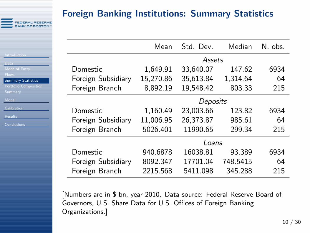
Foreign Banking Institutions: Summary Statistics
Introduction
Data
Mode of Entry
Flows
Summary Statistics
Portfolio Composition
Summary
Model
Calibration
Results
Conclusions
10 / 30
Mean Std. Dev. Median N. obs.
AssetsDomestic 1,649.91 33,640.07 147.62 6934Foreign Subsidiary 15,270.86 35,613.84 1,314.64 64Foreign Branch 8,892.19 19,548.42 803.33 215
DepositsDomestic 1,160.49 23,003.66 123.82 6934Foreign Subsidiary 11,006.95 26,373.87 985.61 64Foreign Branch 5026.401 11990.65 299.34 215
LoansDomestic 940.6878 16038.81 93.389 6934Foreign Subsidiary 8092.347 17701.04 748.5415 64Foreign Branch 2215.568 5411.098 345.288 215
[Numbers are in $ bn, year 2010. Data source: Federal Reserve Board ofGovernors, U.S. Share Data for U.S. Offices of Foreign BankingOrganizations.]

Size Differences: Assets
Introduction
Data
Mode of Entry
Flows
Summary Statistics
Portfolio Composition
Summary
Model
Calibration
Results
Conclusions
11 / 30
05
1015
bn $
1995q4 1997q4 1999q4 2001q4 2003q4 2005q4 2007q4 2009q4
foreign−branch foreign−branch (+due from related institutions)
foreign−subsidiary domestic bank
Average Assets
⇒ Size distributions

Intra-firm Flows
Introduction
Data
Mode of Entry
Flows
Summary Statistics
Portfolio Composition
Summary
Model
Calibration
Results
Conclusions
12 / 30
−1
01
23
bn $
1995q1 2000q1 2005q1 2010q1
Net Due From Head Office Net Due To Head Office
Intrafirm Balances (Average)

Portfolio Composition: Loans-to-Assets Ratio
Introduction
Data
Mode of Entry
Flows
Summary Statistics
Portfolio Composition
Summary
Model
Calibration
Results
Conclusions
13 / 30
.2.3
.4.5
.6bn
$
1995q4 1997q4 1999q4 2001q4 2003q4 2005q4 2007q4 2009q4
foreign−branch foreign−subsidiary
domestic bank
Loans / Assets

Portfolio Composition: Loan Types
Introduction
Data
Mode of Entry
Flows
Summary Statistics
Portfolio Composition
Summary
Model
Calibration
Results
Conclusions
14 / 30
020
4060
8010
0
Domestic Bank Foreign−Subsidiary Foreign−Branch
Loan Portfolio
Commercial & Industrial Real Estate
Other
Stylized Facts
Introduction
Data
Mode of Entry
Flows
Summary Statistics
Portfolio Composition
Summary
Model
Calibration
Results
Conclusions
15 / 30
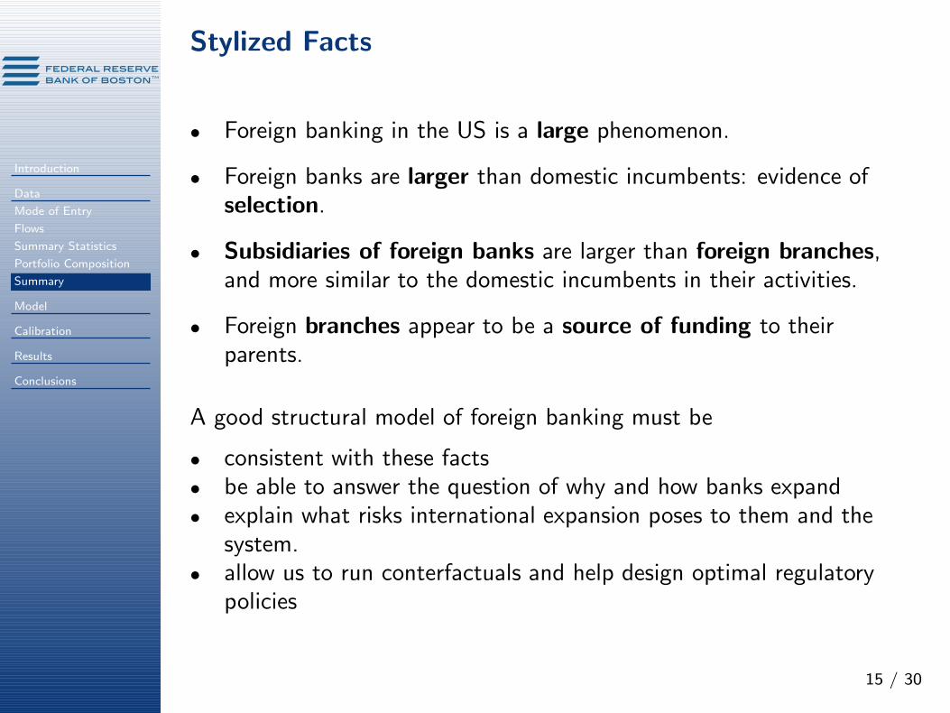
• Foreign banking in the US is a large phenomenon.
• Foreign banks are larger than domestic incumbents: evidence ofselection.
• Subsidiaries of foreign banks are larger than foreign branches,and more similar to the domestic incumbents in their activities.
• Foreign branches appear to be a source of funding to theirparents.
A good structural model of foreign banking must be
• consistent with these facts• be able to answer the question of why and how banks expand• explain what risks international expansion poses to them and the
system.• allow us to run conterfactuals and help design optimal regulatory
policies

The Environment of the Model
Introduction
Data
Model
Setup
Why?
Intra-temporal
Inter-Temporal
Calibration
Results
Conclusions
16 / 30
• Two countries, Home and Foreign (denoted by ∗).
• Time is continuous.
• Each country is populated by a large mass of national banks:
– each bank offers one-period loans (L), makes investments (I) andaccepts deposits (D);
– each bank has some market power in the loans market (start withmonopolistic competition to rule out strategic considerations).
• Study the decision of banks from the Home country to enter theForeign country:
– each bank enters if it can make positive profits in the Foreigncountry;
– the rationale for entry is given by differentiation (spatial or product);– a bank can enter a market either as a branch or as a subsidiary.

The Environment of the Model (contd.)
Introduction
Data
Model
Setup
Why?
Intra-temporal
Inter-Temporal
Calibration
Results
Conclusions
17 / 30
• Banks are heterogeneous in their ability a of managing loans,investments and deposits:
– Each bank has management costs a · C(D,L, I), where C(D,L, I) isa convex function;
– When a bank enters the Foreign market, it transfers his efficiency a tothe subsidiary or branch.
• There are sunk costs of entry, depending on the organizational formof the foreign affiliate: Fs > Fb > 0.
• Loans and investments are risky (on aggregate).
⇓The solution of the optimal entry problem is a bank-specific policyfunction that determines a bank’s entry decision and mode of entry asa function of bank-level characteristics and aggregate variables(aggregate loan demand and return on investments).
Why THIS model?
Introduction
Data
Model
Setup
Why?
Intra-temporal
Inter-Temporal
Calibration
Results
Conclusions
18 / 30
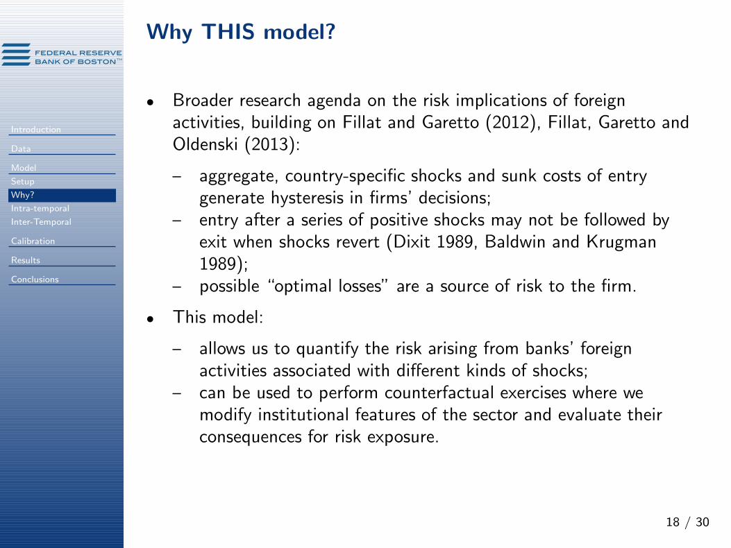
• Broader research agenda on the risk implications of foreignactivities, building on Fillat and Garetto (2012), Fillat, Garetto andOldenski (2013):
– aggregate, country-specific shocks and sunk costs of entrygenerate hysteresis in firms’ decisions;
– entry after a series of positive shocks may not be followed byexit when shocks revert (Dixit 1989, Baldwin and Krugman1989);
– possible “optimal losses” are a source of risk to the firm.
• This model:
– allows us to quantify the risk arising from banks’ foreignactivities associated with different kinds of shocks;
– can be used to perform counterfactual exercises where wemodify institutional features of the sector and evaluate theirconsequences for risk exposure.

Why THIS model?
Introduction
Data
Model
Setup
Why?
Intra-temporal
Inter-Temporal
Calibration
Results
Conclusions
18 / 30
• Broader research agenda on the risk implications of foreignactivities, building on Fillat and Garetto (2012), Fillat, Garetto andOldenski (2013):
– aggregate, country-specific shocks and sunk costs of entrygenerate hysteresis in firms’ decisions;
– entry after a series of positive shocks may not be followed byexit when shocks revert (Dixit 1989, Baldwin and Krugman1989);
– possible “optimal losses” are a source of risk to the firm.
• This model:
– allows us to quantify the risk arising from banks’ foreignactivities associated with different kinds of shocks;
– can be used to perform counterfactual exercises where wemodify institutional features of the sector and evaluate theirconsequences for risk exposure.
• What we CANNOT talk about (yet):
– Maturity mismatch. Liquidity issues are TBA.– Drivers of aggregate shocks in the banking sector.

Intra-temporal Problem: National Banks
Introduction
Data
Model
Setup
Why?
Intra-temporal
Inter-Temporal
Calibration
Results
Conclusions
19 / 30
Determine the optimal per-period profits of a bank given its foreignstatus.
• A national bank chooses the optimal amounts of loans L, depositsD, investment I, interbank borrowing M , and equity E tomaximize its profits πN :
maxL,I,D,M,E
πN = prL(L) · L− (1− p)L+ rII − rDD − rMM − ...
aC(D,L, I)− fp ·D
s.t. M +D + E = L+ I (resource constraint)
E
ωLL+ ωII≥ k (capital requirement).
where p is the probability of loan repayment, fp is the deposit insurancepremium, k is the capital requirement, and ωL, ωI are weights.rL(L) is a downward-sloping demand for loans, while rI , rD, and rM
are taken as given by the bank.

Intra-temporal Problem: Parent + Foreign Sub Pair
Introduction
Data
Model
Setup
Why?
Intra-temporal
Inter-Temporal
Calibration
Results
Conclusions
20 / 30
• In a parent + subsidiary pair, the profit maximization problem ofthe parent in the home country is identical to the problem of anational bank. The foreign subsidiary is operated as an independententity to maximize its profits πS :
maxL∗,I∗,D∗,M∗,E∗
πS = pr∗L(L∗) · L∗ − (1− p)L∗ + rII
∗ − rDD∗ − ...
rMM∗ − aC(D∗, L∗, I∗)− fp ·D∗ − FS
s.t. M∗ +D∗ + E∗ = L∗ + I∗ (resource constraint)
E∗
ωLL∗ + ωII∗≥ k (capital requirement).
Intra-temporal Problem: Parent + Foreign Branch Pair
Introduction
Data
Model
Setup
Why?
Intra-temporal
Inter-Temporal
Calibration
Results
Conclusions
21 / 30
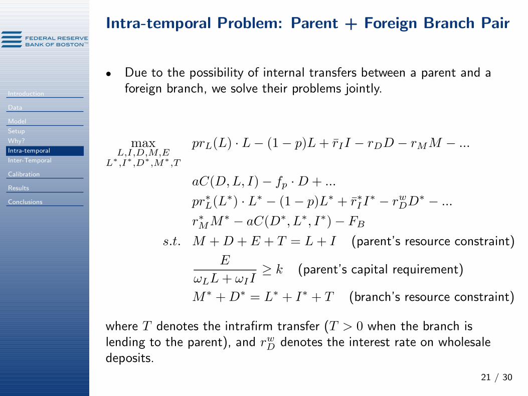
• Due to the possibility of internal transfers between a parent and aforeign branch, we solve their problems jointly.
maxL,I,D,M,E
L∗,I∗,D∗,M∗,T
prL(L) · L− (1− p)L+ rII − rDD − rMM − ...
aC(D,L, I)− fp ·D + ...
pr∗L(L∗) · L∗ − (1− p)L∗ + r∗I I
∗ − rwDD∗ − ...
r∗MM∗ − aC(D∗, L∗, I∗)− FB
s.t. M +D + E + T = L+ I (parent’s resource constraint)
E
ωLL+ ωII≥ k (parent’s capital requirement)
M∗ +D∗ = L∗ + I∗ + T (branch’s resource constraint)
where T denotes the intrafirm transfer (T > 0 when the branch islending to the parent), and rwD denotes the interest rate on wholesaledeposits.
Intra-temporal Problem: Matching Cross-Sectional Facts
Introduction
Data
Model
Setup
Why?
Intra-temporal
Inter-Temporal
Calibration
Results
Conclusions
22 / 30
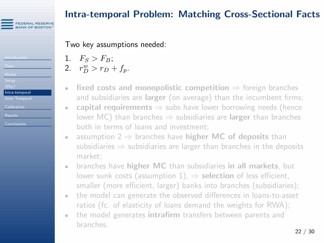
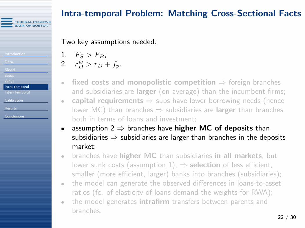
Two key assumptions needed:
1. FS > FB;2. rwD > rD + fp.
• fixed costs and monopolistic competition ⇒ foreign branchesand subsidiaries are larger (on average) than the incumbent firms;
• capital requirements ⇒ subs have lower borrowing needs (hencelower MC) than branches ⇒ subsidiaries are larger than branchesboth in terms of loans and investment;
• assumption 2 ⇒ branches have higher MC of deposits thansubsidiaries ⇒ subsidiaries are larger than branches in the depositsmarket;
• branches have higher MC than subsidiaries in all markets, butlower sunk costs (assumption 1), ⇒ selection of less efficient,smaller (more efficient, larger) banks into branches (subsidiaries);
• the model can generate the observed differences in loans-to-assetratios (fc. of elasticity of loans demand the weights for RWA);
• the model generates intrafirm transfers between parents andbranches.

Intra-temporal Problem: Matching Cross-Sectional Facts
Introduction
Data
Model
Setup
Why?
Intra-temporal
Inter-Temporal
Calibration
Results
Conclusions
22 / 30
Two key assumptions needed:
1. FS > FB;2. rwD > rD + fp.
• fixed costs and monopolistic competition ⇒ foreign branchesand subsidiaries are larger (on average) than the incumbent firms;
• capital requirements ⇒ subs have lower borrowing needs (hencelower MC) than branches ⇒ subsidiaries are larger than branchesboth in terms of loans and investment;
• assumption 2 ⇒ branches have higher MC of deposits thansubsidiaries ⇒ subsidiaries are larger than branches in the depositsmarket;
• branches have higher MC than subsidiaries in all markets, butlower sunk costs (assumption 1), ⇒ selection of less efficient,smaller (more efficient, larger) banks into branches (subsidiaries);
• the model can generate the observed differences in loans-to-assetratios (fc. of elasticity of loans demand the weights for RWA);
• the model generates intrafirm transfers between parents andbranches.

Inter-temporal Model: Aggregation and Shocks
Introduction
Data
Model
Setup
Why?
Intra-temporal
Inter-Temporal
Calibration
Results
Conclusions
23 / 30
Shocks to aggregate loans demand:
dL
L= µdt+ σdz
dL∗
L∗= µ∗dt+ σ∗dz∗
where µ, µ∗ ≥ 0, σ, σ∗ > 0 and dz, dz∗ are the increments of twostandard Wiener processes with correlation ρ ∈ [−1, 1].
Aggregation:
L =
(∫
L1−1/ηdL
)η/(η−1)
where η > 1 is also the elasticity of demand of each individual loantype.
[“Technical” role of these assumptions: ensure that interest rates on loans
are independent of L, and that each bank’s optimal profits in a country are a
linear affine function of L.]

Inter-temporal Model: Bellman Equations
Introduction
Data
Model
Setup
Why?
Intra-temporal
Inter-Temporal
Calibration
Results
Conclusions
24 / 30
Let Vi(a,L,L∗) denote the value of a bank with efficiency a with
international status i (i ∈ {N,B, S}), when aggregate loan demand inthe two markets is described by (L,L∗):
Vi(a,L,L∗) = S(a,L) + Vi(a,L
∗)
where S(a,L) is the expected p.d.v. of domestic profits (independentof i), and Vi(a,L
∗) is the expected p.d.v. of foreign profits for a bankin status i.
Bellman equations:
S(a,L) = πN (a,L) + E[S(a,L′)|L]
VN (a,L∗) = max{
E[VN (a,L∗′)|a,L∗] ; VB(a,L∗)− FB ; ...
VS(a,L∗)− FS}
VB(a,L∗) = max
{
πB(a,L∗) + E[VB(a,L
∗′)|L∗] ; VN (a,L∗)}
VS(a,L∗) = max
{
πS(a,L∗) + E[VS(a,L
∗′)|L∗] ; VN (a,L∗)}

Inter-temporal Model: Value Functions
Introduction
Data
Model
Setup
Why?
Intra-temporal
Inter-Temporal
Calibration
Results
Conclusions
25 / 30
In the continuation regions:
S(a,L) =πN (a,L)
rM
VN (a,L∗) = AN (a)L∗α +BN (a)L∗β
VB(a,L∗) = AB(a)L
∗α +BB(a)L∗β +
πB
r∗M
VS(a,L∗) = AS(a)L
∗α +BS(a)L∗β +
πS
r∗M
where α and β are the roots of: 12σ
∗2ξ2 + (µ∗ − 12σ
∗2)ξ − rM = 0(α < 0, β > 1).
Value-matching and smooth pasting conditions deliver the parametersAi(a) and Bi(a) (i ∈ {N,B, S}) and the thresholds in aggregate loandemand that induce banks to enter or exit the foreign market (thepolicy function).

What does the Simulated Model Do?
Introduction
Data
Model
Setup
Why?
Intra-temporal
Inter-Temporal
Calibration
Results
Conclusions
26 / 30
• Parameterize the model and generate an economy with a largenumber of domestic banks.1
• Simulate the stochastic process describing aggregate loan demandin each country.
• Every period, the model delivers:
1. banks’ endogenous decisions of foreign entry (by type);2. banks’ endogenous decisions of exit from the foreign market (by
type);3. banks’ domestic and foreign flows of deposits, loans,
investment, interbank borrowing, and intrafirm transfers;4. banks’ domestic and foreign profits depending on the mode of
entry;5. banks’ domestic and foreign risk exposure (computed
theoretically as the covariance of a bank’s profits with domesticloan demand).
1Functional form assumptions: C(D,L, I) ≡ βLL+ βII2
2+ βDD2
2and manage-
ment efficiency x ≡ 1/a distributed according to G(x) = 1− bϑx−ϑ.
Calibration
Introduction
Data
Model
Calibration
SMM
Results
Conclusions
27 / 30
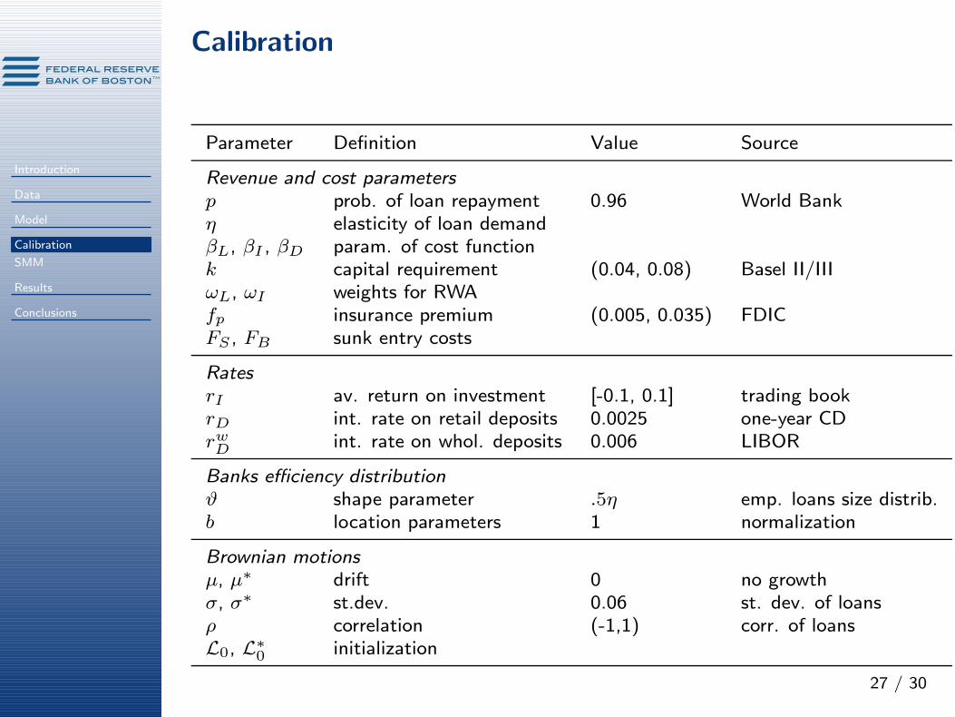
Parameter Definition Value Source
Revenue and cost parameters
p prob. of loan repayment 0.96 World Bankη elasticity of loan demandβL, βI , βD param. of cost functionk capital requirement (0.04, 0.08) Basel II/IIIωL, ωI weights for RWAfp insurance premium (0.005, 0.035) FDICFS , FB sunk entry costs
Rates
rI av. return on investment [-0.1, 0.1] trading bookrD int. rate on retail deposits 0.0025 one-year CDrwD
int. rate on whol. deposits 0.006 LIBOR
Banks efficiency distribution
ϑ shape parameter .5η emp. loans size distrib.b location parameters 1 normalization
Brownian motions
µ, µ∗ drift 0 no growthσ, σ∗ st.dev. 0.06 st. dev. of loansρ correlation (-1,1) corr. of loansL0, L∗
0initialization

Calibration: SMM (ongoing)
Introduction
Data
Model
Calibration
SMM
Results
Conclusions
28 / 30
• Direct calibration of p, k, fp, rI , rD, rwD, ϑ, b, µ, µ∗, σ, σ∗, ρ.
• Remaining 10 parameters: η, βL, βI , βD, ωL, ωI , FS , FB, L0, L∗
0
calibrated jointly to match moments from the data:
– average interest rates on loans (1 moment);– relative size of deposits and loans in branches compared to
subsidiaries (2 moments);– relative loans-to-assets ratios in branches compared to
subsidiaries (1 moment);– percentages of branches and subsidiaries in the total number of
banks in the US (2 moments);– entry and exit dynamics: average share of national banks that
become branches (subsidiaries) each year, and average share ofbranches (subsidiaries) exiting each year (4 moments).

Results and Extensions
Introduction
Data
Model
Calibration
Results
Conclusions
29 / 30
Use the model to evaluate the following counterfactual scenarios:
• changes in deposit insurance and capital requirements rules;• extending interbank transfers to subsidiaries;• elimination of the possibility of opening branches or subsidiaries.
Extensions:
• stochastic rates of return on investments;• shocks to deposits supply.

Conclusions
Introduction
Data
Model
Calibration
Results
Conclusions
30 / 30
• Growing interest (and literature!) on the operations ofmultinational banks.
• In this paper we provide a structural model that is designed toreproduce features of the foreign banking sector, includingendogeneity of entry decisions and the choice of the mode of entry.
• The model has the potential to become a laboratory to conductpolicy analysis.

History of Banking Regulation
Introduction
Data
Model
Calibration
Results
Conclusions
Appendix
Regulation
Size differences
Parameterization
31 / 30
• 1927 – McFadden Act prohibits interstate banking.
• 1978 – International Banking Act:
– brings foreign banks within the federal regulatory framework,– requires deposit insurance for branches of foreign banks engaged
in retail deposit taking in the U.S.
• 1991 – FBSEA (Foreign Bank Supervision Enhancement Act), partof FDICIA (Federal Deposit Insurance Corporation ImprovementAct):
– eliminates deposit insurance for branches of foreign banks.
• 1994 – Riegle-Neal Interstate Banking and Branching EfficiencyAct:
– adequately capitalized and managed Bank Holding Companies(BHCs) are permitted to acquire banks in any state. The law isthe same for both domestic and international banks.
Size Distributions
Introduction
Data
Model
Calibration
Results
Conclusions
Appendix
Regulation
Size differences
Parameterization
32 / 30
0.2
.4.6
.81
F
0 5 10 15 20Log of Total Deposits
Foreign−Subsidiaries Foreign−Branches
Source: only foreign−owned institutions
Date: Q4/2010Cumulative Size Distribution − Deposits
0.2
.4.6
.81
F
5 10 15 20Log of Total Loans
Foreign−Subsidiaries Foreign−Branches
Source: only foreign−owned institutions
Date: Q4/2010Cumulative Size Distribution − Loans
0.2
.4.6
.81
F
0 5 10 15 20Log of Total Assets
Foreign−Subsidiaries Foreign−Branches
Source: only foreign−owned institutions
Date: Q4/2010Cumulative Size Distribution − Assets
On Modeling Deposit Insurance
Introduction
Data
Model
Calibration
Results
Conclusions
Appendix
Regulation
Size differences
Parameterization
33 / 30
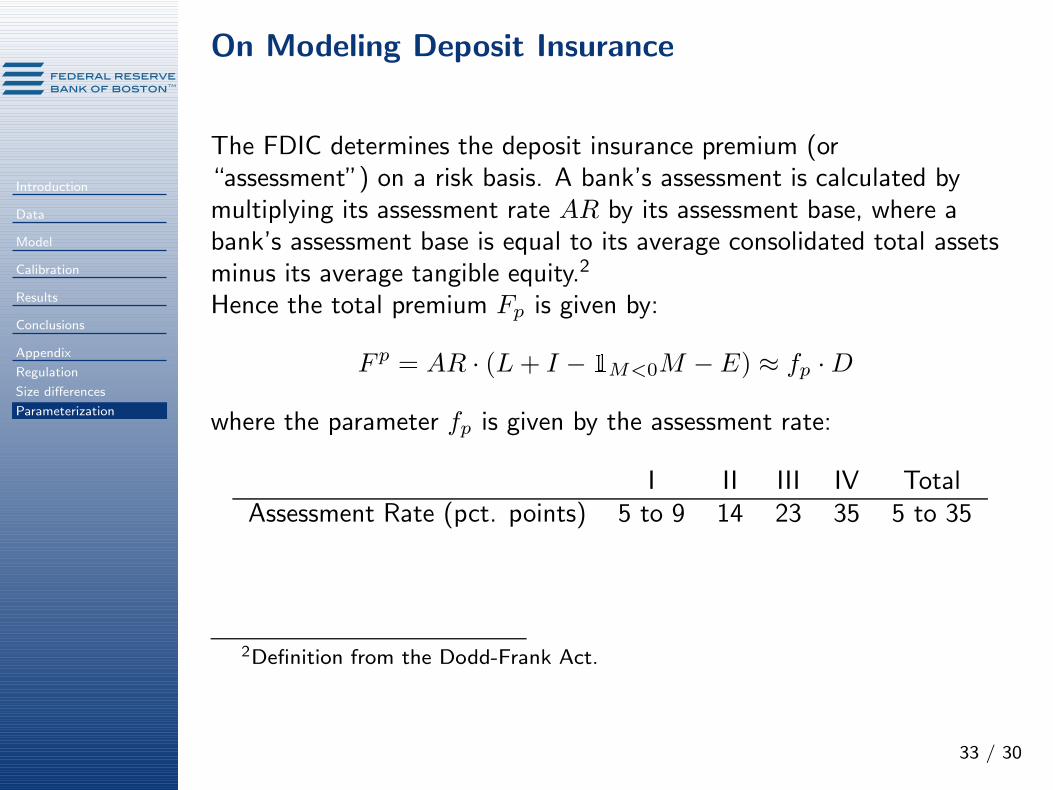
The FDIC determines the deposit insurance premium (or“assessment”) on a risk basis. A bank’s assessment is calculated bymultiplying its assessment rate AR by its assessment base, where abank’s assessment base is equal to its average consolidated total assetsminus its average tangible equity.2
Hence the total premium Fp is given by:
F p = AR · (L+ I − 1M<0M − E) ≈ fp ·D
where the parameter fp is given by the assessment rate:
I II III IV TotalAssessment Rate (pct. points) 5 to 9 14 23 35 5 to 35
2Definition from the Dodd-Frank Act.
On the Loan Size Distribution
Introduction
Data
Model
Calibration
Results
Conclusions
Appendix
Regulation
Size differences
Parameterization
34 / 30
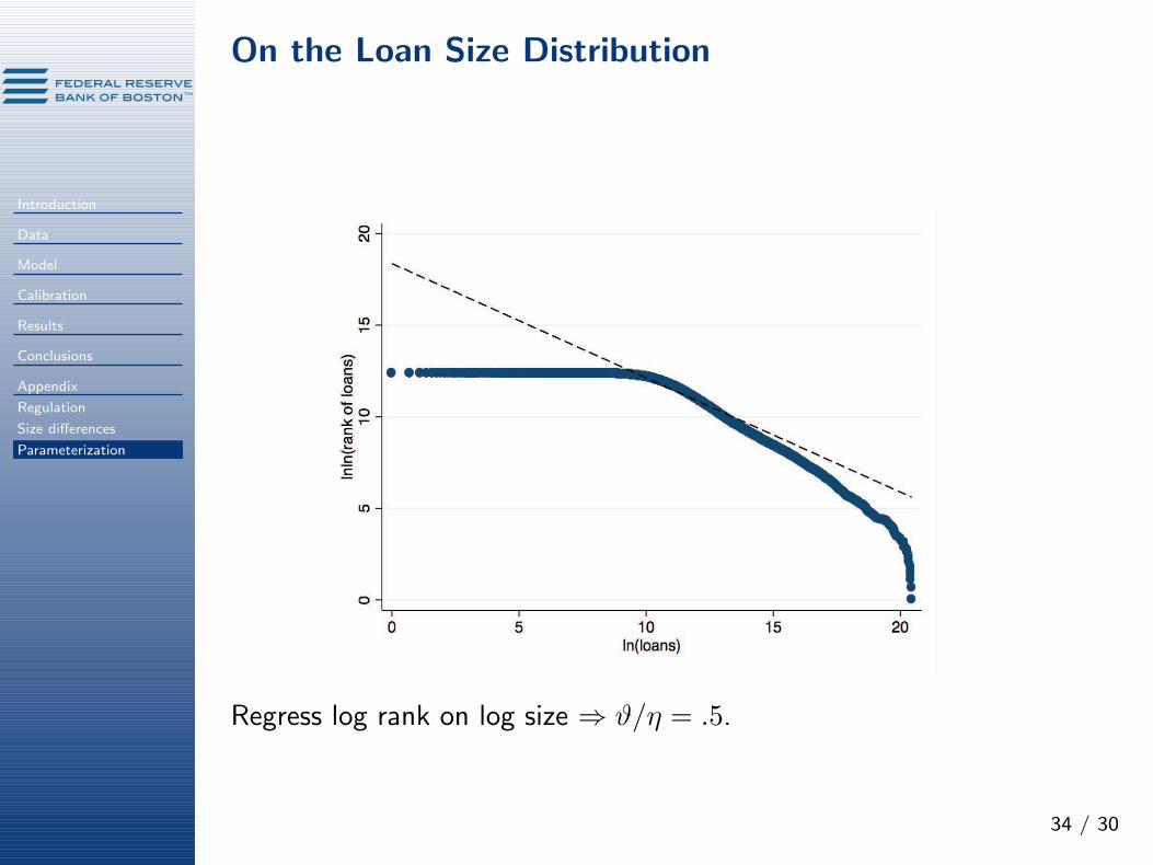
Regress log rank on log size ⇒ ϑ/η = .5.
Recommended