
Introduction MI methods for multilevel data Comparisons Conclusion References
Multiple imputation for multilevel data withcontinuous and binary variables
V. Audigier, I. White , S. Jolani, T. Debray, M. Quartagno, J.Carpenter, S. van Buuren, M. Resche-Rigon
CEDRIC, MSDMA team, CNAM, Paris
Chimiometrie XIX, 2018 January 31st, Paris
1 / 15

Introduction MI methods for multilevel data Comparisons Conclusion References
Motivation: GREAT data (GREAT Network, 2013)
• Risk factors associated with short-term mortality in acuteheart failure
• 28 observational cohorts,11685 patients, 2 binary and 8continuous variables (patientcharacteristics and potentialrisk factors)
• sporadically and systematicallymissing data
Y1,Y2,Y3, ... Yp−1,Yp
gend
er bmi
age
SBP
DBP HR bnpl
AFib
LVEF
Inde
x
Aim: explain the relationship between biomarkers (BNP, AFIB,...)and the left ventricular ejection fraction (LVEF)
yLVEFik = β0 + β1yBNPik + β2yAFIBik + b0
k + b1ky
BNPik + εik
bk ∼ N (0,Ψ) εik ∼ N(0, σ2)
β and associated variability var(β)
2 / 15

Introduction MI methods for multilevel data Comparisons Conclusion References
Multiple imputation (Rubin, 1987)
1 Generate a set of M parameters (θm)1≤m≤M of an imputationmodel to generate M plausible imputed data sets
P(Ymiss |Y obs , θ1
). . . . . . . . . P
(Ymiss |Y obs , θM
)(F u′)ij (F u′)1ij + ε
1
ij (F u′)2ij + ε2
ij(F u′)3ij + ε
3
ij (F u′)Bij + εBij
2 Fit the analysis model on each imputed data set: βm, Var(βm
)3 Combine the results: β = 1
M
∑Mm=1 βm
Var(β)
= 1M
∑Mm=1 Var
(βm
)+(1 + 1
M
) 1M−1
∑Mm=1
(βm − β
)2
⇒ Provide estimation of the parameters and of their variability
3 / 15

Introduction MI methods for multilevel data Comparisons Conclusion References
Imputation model for multilevel data
Two standard ways to perform MI
• Fully conditional specification (FCS, MICE): a conditional imputationmodel for each variable
• Joint modelling (JM): a joint imputation model for all variables
The imputation model (joint or conditional) needs to
• account for the heterogeneity between clusters
• account for the types of variables (continuous and binary)
• be identifiable with sporadically and systematically missing values
4 / 15
Introduction MI methods for multilevel data Comparisons Conclusion References
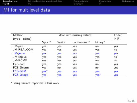
MI for multilevel data
Method(type - name)
deal with missing values: Codedin R
Spor.? Syst.? continuous ? binary?JM-pan yes yes yes no yesJM-REALCOM yes yes yes yes noJM-jomo yes yes yes yes yesJM-Mplus yes yes yes yes noJM-RCME yes yes yes no noFCS-pan yes yes yes no yesFCS-2lnorm yes no yes no yesFCS-GLM yes∗ yes yes yes yesFCS-2stage yes yes yes yes∗ yes
∗ using variant reported in this work
5 / 15
Introduction MI methods for multilevel data Comparisons Conclusion References
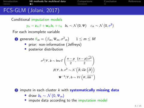
FCS-GLM (Jolani, 2017)
Conditional imputation modelsyik = zikβ + wikbk + εik bk ∼ N (0,Ψ) εik ∼ N
(0, σ2)
For each incomplete variable
1 generate θm =(βm,Ψm, σ
2m
)1 ≤ m ≤ M
• prior: non-informative (Jeffreys)• posterior distribution
σ2|Y , b ∼ Inv-Γ
(n − p
2,
(n − p) σ2
2
)β|Y , b, σ2 ∼ N
(β, var
(β))
Ψ−1|Y , b ∼ W(K , bb>
)
2 impute in each cluster k with systematically missing data• draw bk ∼ N (0,Ψm)• impute data according to the imputation model
6 / 15

Introduction MI methods for multilevel data Comparisons Conclusion References
FCS-GLM (Jolani, 2017)
Conditional imputation modelsyik = zikβ + wikbk + εik bk ∼ N (0,Ψ) εik ∼ N
(0, σ2)
For each incomplete variable
1 generate θm =(βm,Ψm, σ
2m
)1 ≤ m ≤ M
• prior: non-informative (Jeffreys)• posterior distribution
σ2|Y , b ∼ Inv-Γ
(n − p
2,
(n − p) σ2
2
)β|Y , b, σ2 ∼ N
(β, var
(β))
Ψ−1|Y , b ∼ W(K , bb>
)
2 impute in each cluster k with sporadically missing data• draw bk ∼ N
(µbk |yk ,Ψbk |yk
)• impute data according to the imputation model
6 / 15

Introduction MI methods for multilevel data Comparisons Conclusion References
Differences between MI methods
Prior heteroscedasticityassumption
linkbinary
FCS-GLM Jeffrey no logitFCS-2stage yes logitJM-jomo conjugate yes probit
• conjugate prior distributions are known to very informative inGLMM• heteroscedastic assumption is more flexible
7 / 15
Introduction MI methods for multilevel data Comparisons Conclusion References
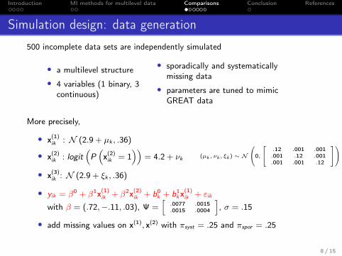
Simulation design: data generation
500 incomplete data sets are independently simulated
• a multilevel structure• 4 variables (1 binary, 3
continuous)
• sporadically and systematicallymissing data
• parameters are tuned to mimicGREAT data
More precisely,
• x(1)ik : N (2.9 + µk , .36)
• x(2)ik : logit
(P(x(2)ik = 1
))= 4.2 + νk
• x(3)ik : N (2.9 + ξk , .36)
(µk , νk , ξk ) ∼ N
0,
.12 .001 .001.001 .12 .001.001 .001 .12
• yik = β0 + β1x(1)ik + β2x(2)
ik + b0k + b1
kx(1)ik + εik
with β = (.72,−.11, .03), Ψ =[.0077 .0015.0015 .0004
], σ = .15
• add missing values on x(1), x(2) with πsyst = .25 and πspor = .25
8 / 15
Introduction MI methods for multilevel data Comparisons Conclusion References
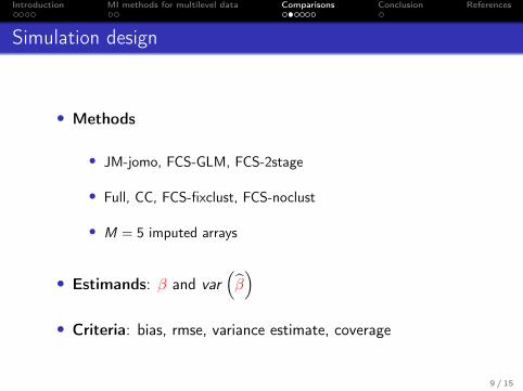
Simulation design
• Methods
• JM-jomo, FCS-GLM, FCS-2stage
• Full, CC, FCS-fixclust, FCS-noclust
• M = 5 imputed arrays
• Estimands: β and var(β)
• Criteria: bias, rmse, variance estimate, coverage
9 / 15

Introduction MI methods for multilevel data Comparisons Conclusion References
Results: base-case
β−β
Full CC
FCS−
noclu
st
FCS−
fixclus
t
FCS−
GLM
FCS−
2stag
e
JM−jo
mo
−0.02
−0.01
0.00
0.01
0.02 β1
β2
Method√
var(β) √
var(β)
95% Cover Time (min)
β1 β2 β1 β2 β1 β2Full 0.0047 0.0029 0.0048 0.0030 93.8 94.2CC 0.0070 0.0053 0.0071 0.0053 92.2 94.4FCS-noclust 0.0041 0.0043 0.0067 0.0045 58.2 92.0 0.9FCS-fixclust 0.0043 0.0043 0.0058 0.0042 87.0 94.6 1.1FCS-GLM 0.0047 0.0046 0.0057 0.0043 89.7 95.8 103.3FCS-2stage 0.0059 0.0049 0.0058 0.0044 95.0 96.2 0.9JM-jomo 0.0066 0.0069 0.0056 0.0049 98.4 97.6 7.8
10 / 15

Introduction MI methods for multilevel data Comparisons Conclusion References
Influence of the number of clusters
●
●●
−2
0−
15
−1
0−
50
β(1)
K
Re
lative
bia
s (
%)
● JM−jomoFCS−GLMFCS−2stage
7 14 28
●
●
●
−2
0−
15
−1
0−
50
β(2)
K
Re
lative
bia
s (
%)
● JM−jomoFCS−GLMFCS−2stage
7 14 28
11 / 15
Introduction MI methods for multilevel data Comparisons Conclusion References
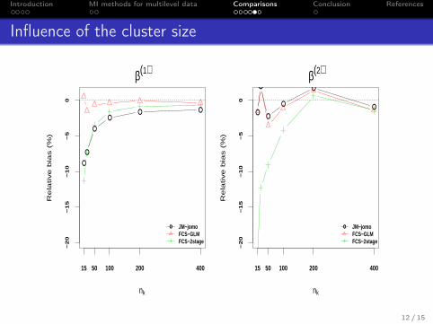
Influence of the cluster size
●●●
●
●
●
−2
0−
15
−1
0−
50
β(1)
nk
Re
lative
bia
s (
%)
● JM−jomoFCS−GLMFCS−2stage
15 50 100 200 400
●
●
●
●
●
●
−2
0−
15
−1
0−
50
β(2)
nk
Re
lative
bia
s (
%)
● JM−jomoFCS−GLMFCS−2stage
15 50 100 200 400
12 / 15

Introduction MI methods for multilevel data Comparisons Conclusion References
Influence of the proportion of systematically missing values
●
●
●
0.0
04
50
.00
55
0.0
06
50
.00
75
0.10 0.25 0.40πsyst
0.375 0.25 0.0625πspor
●●
●
● model se JM−jomomodel se FCS−GLMmodel se FCS−2stage
●
●
●
0.0
05
0.0
06
0.0
07
0.0
08
0.10 0.25 0.40πsyst
0.375 0.25 0.0625πspor
●
●
●
● model se JM−jomomodel se FCS−GLMmodel se FCS−2stage
13 / 15

Introduction MI methods for multilevel data Comparisons Conclusion References
Conclusion
An overview of MI methods for multilevel data
• FCS-GLM, FCS-2stage and JM-jomo all appear to perform well• Outperform had-hoc methods
FCS-2stage • provides a quick way to obtain first results• for large clusters
FCS-GLM • tends to underestimate the variance of the estimatorbecause of the homoscedastic assumption
• recommended with small clusters• time consuming (with binary variables)
JM-jomo • tends to overestimate the variance of the fixedcoefficients because of unsuitable prior distributions
• recommended for large clusters when the proportion ofbinary variables is high
Methods are implemented in R packages (mice, micemd, jomo)
14 / 15

Introduction MI methods for multilevel data Comparisons Conclusion References
References I
Global Research on Acute conditions Team (GREAT) Network. Managing Acute Heart Failure in theED - Case Studies from the Acute Heart Failure Academy, 2013. http://www.greatnetwork.org.
D. Rubin. Multiple Imputation for Non-Response in Survey. Wiley, New-York, 1987.
S. Jolani. Hierarchical imputation of systematically and sporadically missing data: An approximatebayesian approach using chained equations. Biometrical Journal, 2017. doi:10.1002/bimj.201600220.
V. Audigier, I. R. White, S. Jolani, T. P. A. Debray, M. Quartagno, J. Carpenter, S. van Buuren, andM. Resche-Rigon. Multiple imputation for multilevel data with continuous and binary variables.ArXiv e-prints, 2017.
V. Audigier and M. Resche-Rigon. micemd: Multiple Imputation by Chained Equations with MultilevelData, 2017. R package version 1.2.0.
M. Quartagno and J. Carpenter. jomo: A package for Multilevel Joint Modelling Multiple Imputation,2016. URL http://CRAN.R-project.org/package=jomo. R package version 2.2-0.
Matthieu Resche-Rigon and Ian White. Multiple imputation by chained equations for systematically andsporadically missing multilevel data. Statistical Methods in Medical Research, 2016.http://dx.doi.org/10.1177/0962280216666564.
15 / 15
Recommended


![[ME] Multilevel Mixed Effects - Stata · PDF file[XT] Stata Longitudinal-Data/Panel-Data Reference Manual [ME] Stata Multilevel Mixed-Effects Reference Manual [MI] Stata Multiple-Imputation](https://img.pdfslide.net/doc/110x75/5a78a96c7f8b9a7b698e4b38/me-multilevel-mixed-effects-stata-xt-stata-longitudinal-datapanel-data-reference.jpg)


![[MI] Multiple Imputation - Stata](https://img.pdfslide.net/doc/110x75/62039c6dda24ad121e4b6a82/mi-multiple-imputation-stata.jpg)