N94-14621
Some Experiences with Krylov Vectors andLanczos Vectors
Roy R. Craig, Jr.', Tzu-Jeng Su t, and Hyoung M. Kim _
This paper illustrates the use of Krylov vectors and Lanczos vectors
for reduced-order modeling in structural dynamics and for control of flex-
ible structures. Krylov vectors and Lanczos vectors are defined and illus-
trated, and several applications that have been under study at The Univer-
sity of Texas at Austin are reviewed: model reduction for undamped struc-
tural dynamics systems, component mode synthesis using Krylov vectors,
model reduction of damped structural dynamics systems, and one-sided
and two-sided unsymmetric block-Lanczos model-reduction algorithms.
1. Introduction
In recent years extensive research has been carried out on Lanczos eigensolution
algorithms (see, for example, Refs. [1, 2]). Nour-Omid and Clough [3] demonstrated the
usefulness of Lanczos vectors in the analysis of the dynamic response of structures, and
Frisch [4] included Lanczos vectors among the sets of Ritz vectors that are available
in the DISCOS multibody code. Research has involved single-vector and block-vector
methods, algorithms based on first-order equations of motion and algorithms based
on second-order equations, and algorithms for unsymmetric matrices as well as for
symmetric matrices.
Following a brief introduction to the physical meaning of Krylov vectors and
Lanczos vectors, this paper summarizes several applications that have been under
study recently at The University of Texas at Austin.
Structural dynamicists are all familiar with the fact that the modes of free
vibration of an undamped structure (modeled, for example, as an n-degree-of-freedom
finite element model) satisfy the algebraic eigenproblem
K¢, = A,M¢, r = 1,2,...,n (1)
"John J. McKetta Energy Professor of Engineering, Department of Aerospace Engineering and
Engineering Mechanics, The University of Texas at Austin, Austin, TX 78712-1085.t National Research Council Research Associate, NASA Langley Research Center, Spacecraft
Dynamics Branch, Hampton, VA 23665-5225._Technical Specialist, McDonnell Douglas Space Systems Company, Space Station Division, Hous-
ton, TX 77062.
PRECEDING PAGE BLANK NOT FILMED
37
https://ntrs.nasa.gov/search.jsp?R=19940010148 2018-07-30T02:29:53+00:00Z

where K, M, .k,, and Cr are, respectively, the stiffness matrix, mass matrix, r-th
eigenvalue, and r-th eigenvector. However, Krylov vectors and Lanczos vectors are
not as well known as are eigenvectors. Note that Eq. (1) is basically an equilibrium
equation relating elastic restoring forces, KCr, to inertia forces JM¢,, and recall
that a modification of Eq. (1), namely
K¢ (j+l) = Me (j) (2)
is the basis for the inverse iteration method for computing eigenvalues and eigenvec-
tots [5]. The vector ¢ in Eq. (2) converges to the fundamental mode (eigenvector) or,
with suitable orthogonalization with respect to tower-frequency modes, to a higher-
frequency mode. Equation (2) states that, given a vector ¢0), a new vector ¢0+,)
may be generated by solving for the static deflection produced by the inertia forces
associated with ¢O), that is,
¢(J+') = If-' [Me (j)] (3)
(assuming that K is nonsingular). Equation (3) provides a basis for defining a Krylov
subspace.
Given a starting vector ¢_), the vectors ¢_) are said to form a Krylov subspace
of order p, 1 < p < n, given by
07)_= [¢_), [K-'MI¢_ ), [K-'M]2¢_ }, ..., [K-'MI('-')¢_ )] (4)
Lanczos vectors differ from the Krylov vectors defined in Eq. (4) in that each Lanczos
vector is made orthogonal to the previous two Lanczos vectors, and it can be shown
that this makes the present Lanczos vector (theoretically) orthogonal to all prior
vectors.
The following algorithm may be used to compute Lanczos vectors for an un-
damped system. Let ¢_01 = 0, and select a starting vector ¢_0. The algorithm to0+,)
compute the Lanczos vector ¢L may be expressed by the following equations:
_(J) = K-'M¢O}
= _ _
where
% = ¢?)VM_./j)
_+_)_ 1 ¢(j)flj+,
(5)
_J
38

and1
Note that the only step in the algorithm, Eq. (5), that distinguishes Lanczos
vectors from Krylov vectors is the orthogonalization step, and note that the mass
matrix M is used in the orthonormalization step above.
Figure 1. A 4-DOF Cantilever Beam Finite Element Model.
Figure 1 shows a four degree-of-freedom (4-DOF) finite element model for a
cantilever beam that is used to illustrate Krylov vectors and Lanczos vectors. Figure 2
shows the four Krylov vectors generated from a starting vector that is the static
deflection due to a unit force at the tip. Figure 3 shows the four Lanczos vectors for
the cantilever beam of Fig. 1. The starting vector, ¢(L11, is the same static deflection
due to a unit tip force which was used as the starting Krylov vector in Fig. 2. Because
the starting vector produces a shape that resembles closely the fundamental mode of
the cantilever beam, the subsequent Lanczos vectors in Fig. 3 resemble the second
o 2 o0 0.5 1 1_ 2 0 0.5 1 1.5 2
6
00 0.5 I 1.5
o
02 "_ 0 0.5 I 1.5 2
Figure 2. The Four I(rylov Vectors for the 4-DOF Cantilever Beam.
39

1...1 . ,-1
0 0.5 1 1.5 2 0 0.5 1 1.5 2
Figure
NO
,..1 .
e_0 0.5 1 1.5 2
3. The Four Lanczos Vectors for
0 ---
"_ 0 0.5 1 1.5 2
the 4-DOF Cantilever Beam.
through fourth normal modes (eigenvectors).
A Krylov subspace of order p is a p-dimensional vector space spanned by thecolumns of the matrix
(I)(p) = [¢, A¢, A2¢, ..., A(P-')¢] (6)
where A is an n x n-dimensional matrix and ¢ is any n-dimensional starting vector.
Depending on the choice of A and ¢, the basis vectors in Eq. (6) are either linearly
dependent for some p < n, or they span the entire n-dimensional space when p = n.
If the vector ¢ is replaced by a matrix with q linearly-independent columns rather
than a single column, the subspace _ is called a biock-Krylov subspace.
2. Lanczos Model Reduction for Undamped Structural Dynamics
Systems (Refs. [6,7])
Some studies have shown that Krylov/Lanczos-based reduced-order models pro-
vide an alternative to normal-mode (eigenvector) reduced-order models in application
to structural control problems. For such applications, an undamped structural dy-
namics system can be described by the input-output equations
Mk + Kx = Pu
y = vz + (7)
where x E R" is the displacement vector; u E R l is the input vector; y E R m is the
output measurement vector; M and I( are the system mass and stiffness matrices;
40

P is the force distribution matrix; and V and W are the displacement and velocity
sensor distribution matrices. In most practical cases, we can assume that I and m are
much smaller than n.
Model reduction of structural dynamics systems is usually based on the Rayleigh-
Ritz method of selecting an n × r transformation matrix L such that
x = L_ (8)
where _ E R r (r < n) is the reduced-order vector of (physical or generalized) coordi-
nates. Then, the reduced system equation is
+ =
y = + (9)
where _ = LTML, 7_ = LTKL, 7_ = LTp, ]7 = VL, and "[317= WL. The projection
matrix L can be chosen arbitrarily. Here, however, we choose L to be formed by a
particular set of Krylov vectors. It is shown in Ref. [7] that the resulting reduced-order
model matches a set of parameters called low-frequency moments.
For a general linear system
= Az + Bu
y = Cz
zE F_, uER t
YE R_ (10)
the low-frequency moments are defined by CA-_B, i = 1,2,..., which are the coef-
ficient matrices in the Taylor series expansion of the system transfer function [8,9].
Applying the Fourier transform to Eq. (7a) yields the frequency response solution
X(w) = (g -w2M)-lPV(w), with X(w) and U(w) the Fourier transforms of x and
u. If the system is assumed to have no rigid-body motion, then a Taylor expansion
of the frequency response around w = 0 is possible. Thus,
oo
X(w) = (I-JK-1M)-1K-1PU(w) = _ w2i(g-lM)iK-lPg(w) (11)i=0
Combining Eq. (7b) and Eq. (11), the system output frequency response can be
expressed as
oo
Y(w) = y_[V(K-'M)'K-1P + jwW(K-_M)'K-'P]w_'U(w) (12)i=0
In these expressions, V(K-1M)iK-1P and W(K-IM)iK-IP play roles similar to
that of low-frequency moments in the first-order state-space formulation. To obtain
the reduced-order model of Eq. (9) let
span {L} = span {Lp nv Lw} (13)
41

where
Lp= [ K-'P (K-'M)K-'P ... (K-'M)"K-'P ]
Lv= [ K-iV T (K-'M)K-'V r "'" (K-'M)qK-'VT] (14)
Lw= [ K-'W r (K-'M)K-'W r "" (K-aM)'K-XWr ]
for p, q, s > 0. Then the reduced system matches the low frequency moments
V(K-tM)iK-IPfori = 0, 1, ..., p+q+l and W(K-_M)iK-lP, fori = O, 1, 2, ...,
p+s+l.
The Lp matrix above is the generalized controllability matrix, and the Lv and
Lw matrices are the generalized observability matrices of the dynamic system de-
scribed by Eq. (7). The vectors contained in Lp are Krylov vectors that are generated
in block form by
Q1 = K -1P
Q,+I = K-lMQ_
The first vector block, K-IP, is the system's static deflection due to the force distri-
bution P. The vector block Q,+l can be interpreted as the static deflection produced
by the inertia force associated with the Q,. If only the dynamic response simulation
is concerned, we would choose L = Lp. In this case, the reduced model matches p+ 1
low-frequency moments. As to the vectors in Lv and Lw, a physical interpretation
such as the "static deflection due to sensor distribution" may be inadequate. How-
ever, from an input-output point of view, Lv, Lw, and Lp are equally important as
far as parameter-matching of the reduced-order model is concerned.
Based on Eq. (13), the following algorithm may be used to generate a Krylov
basis that produces a reduced-order model with the stated parameter-matching prop-
erty.
Krylov/Lanczos Algorithm
(1) Starting block of vectors:
(a) Q0 = 0
(b) R0 = K-'/5, /5 = linearly-independent portion of[P V r W r]
(c) P_KR0 = UoEoUo r (singular-value decomposition)
(2)
(d) Q, = RoU0_;½
For j = 1, 2, ..., k - l, repeat:
(e) 7_ = li -_ MQj
(f) Rj = 7_ - Q_Aj - Q___Bj]
A, =Q_Un,,
(normalization)
(orthogonalization )
B, =U,_,__,
42

(g) RrKRj = UjEjUf (singular-value decomposition)
(h) Q./+I = RjBj -r = RjUjE_ _; (normalization)
(3) Form the k-block projection matriz L = [ Q1 Q2 "'" Qk ].
This algorithm is a Krylov algorithm, because the L matrix is generated by a Krylov
recurrence formula (Step e). It is a Lanczos algorithm because the orthogonaliza-
tion scheme is a three-term recursion scheme (Step f). Although the three-term
recursion scheme is a special feature of the Lanczos algorithm, in practice, complete
reorthogonalization or selective reorthogonalization is necessary to prevent the loss
of orthogonality [10-12].
If the projection matrix L generated by the above algorithm is employed to
perform model reduction, then the reduced-order model matches the low-frequency
moments V(K-tM)iK-1P and W(K-IM)iK-_P, for i = 0, 1, 2, ..., 2k - 1.
It can also be shown that the reduced-order model approximates the lower natural
frequencies of the full-order model.
One interesting feature of the transformed system equation in Krylov/Lanczos
coordinates is that it has a special form. Because of the special choice of start-
ing vectors, K-orthogonalization, and three-term recurrence, the transformed system
equation has a mass matrix in block-tridiagonal form, a stiffness matrix equal to the
identity matrix, and force distribution and measurement distribution matrices with
nonzero elements only in the first block. The transformed system equation has the
form× × ×
0
0
_+_=. • u
0
X
X X
X X X
X X
(15)
v=[x 0 0 ... 0]e+[× 0 0 ... 0]}where x denotes the location of nonzero elements. This special form reflects the
structure of a tandem system (Fig. 4), in which only subsystem 5"1 is directly con-
trolled and measured while the remaining subsystems, Si, i = 2, 3, ..., are excited
through chained dynamic coupling. In control applications, as depicted in Ref. [13],
this tandem structure of the dynamic equation eliminates the control spillover and
the observation spillover, but there is still dynamic spillover. For dynamic response
calculations, the block-tridiagonal form can lead to an efficient time-step solution and
can save storage.
43

Figure 4. The Structure of a Tandem System.
3. Lanczos Model Reduction for Damped Structural Dynamics Systems
(Refs. [6,13])
The previous model-reduction strategy can be extended to damped structural
dynamics systems, which are described by the linear input-output equations
M_ + Dk + Kx = Pu
y = Vx + Wk, (16)
To arrive at an algorithm for constructing a reduced-order model that matches
low-frequency moments, it is easier to start from the first-order formulation. The
first-order differential equation equivalent to Eq. (16) can be expressed as
or
with
I= [v w](17)
,f/:; + Rz = Pu
y=?z (18)
, , , -tv ,19,It is possible to reduce Eq. (18) to the standard first-order state-space form and to
derive a projection subspace based on this standard state space form. However, as
shown in Ref. [13], there are significant advantages in using the generalized first-order
form of Eq. (18). This leads to the following recurrence formula for the Krylov blocks:
(20)QY+, I 0 Qy
44

Superscriptsd and v denote displacement and velocity portions of the vector, respec-
tively. The matrix containing the generated vector sequence is called a Krylov matrix.
It has the form
]O_ Q_ O_
Krylov subspaces that are generated by Eq. (20) and that have the above form produce
a projection subspace L that has the desired moment-matching property [13]. Let
Let
LP= [ Q_O Q_Q_ Q_Qd3.'"..Qp_,Q_]d (21a)
be the sequence of vectors generated by Eq. (20) with /_-1/_ the starting block of
vectors, i.e., Q_ = K-' P, Q'_ = O, and let
[ P_ P_ Pad "'" P_q ]L_. =P_ P_ P_ ... P:_,
(21b)
be the subspace of vectors generated by Eq. (20) with /(-1V the starting block of
vectors, i.e., P_ = K-IV T, P_ = -M-IW T. If the projection matrix L is chosensuch that
span {L}=span { Qtd ... Q_ P_ ... pd p_, } (22)
then the reduced-order model of the damped structural dynamics system matches
the system parameters f'([i -137/)'K -_P, for i = 0, 1, ..., p + q- 1. Reference [13]
provides a Lanczos algorithm, similar to the above algorithm for undamped systems,
that produces the desired projection matrix L. The vectors are K-normalized.
Reference [13] contains a model-reduction impulse response example and an
example that illustrates the use of the Krylov/Lanczos reduced model for flexible
structure control. Figure 5 shows the 48-DOF plane truss structure used in the
model-reduction example, and Fig. 6 shows the impulse response based on eight
Krylov vectors versus the impulse response based on the original full-order (48-DOF)
model.
4. A Block-Krylov Component Synthesis Method for Structural Model
Reduction (Ref. [14])
The previous discussions of Krylov/Lanczos model reduction have been applied
to complete structures. Reference [14] describes a block-Krylov model reduction algo-
rithm for structural components, providing "component modes" comparable to those
that are utilized in Refs. [15-19]. The Krylov model-reduction methods described in
Ref. [14] should also be applicable to flexible multibody dynamics formulations.
45
2@15--30 -!
#A = 1.6E*04 EA=8.0E + I 0
Figure 5. Details of a Plane Truss Structure for Model Reduction Example.
xlO-_8
r_
6
4
2
-2
-4
Solid: Full-order model
Dashed: Reduced-order model
¢I l
0 0.1 0.2 0.3 0.4 0.5 0.6
TIME
Figure 6. Impulse Response: Eight Damped Krylov Modes and Exact Solution.
46

CICtCtCICICICICICICtC1CI• • • I •" • 1 • • • I
a. Structural Component and the Complete System.
e i r
C1 C_ CI CI CII I
b. Interior (i) and Boundary (b) Coordinates of a Component.
Figure 7. A Typical Component and Coupled System.
Figure 7 shows a typical component and a corresponding system of coupled
components. The equation of motion for a single undamped component can be written
in the partitioned form
Mb, Mbb _b + Kb_ Kbb z_ = fb (23)
Reference [14] describes both free-interface Krylov modes (related to the Rubin method
of Refs. [17,18]) and fixed-interface Krylov modes (related to the method of Hurty
[19] and Craig and Bampton [15]). Only the latter will be reviewed here.
A constraint mode is defined as the static deflection of a structure when a
unit displacement is applied to one coordinate of a specified set of coordinates, while
the remaining coordinates of that set are restrained and the remaining degrees of
freedom of the structure are force-free. The starting block of vectors for the fized-
interface Krvlov component synthesis method consists of constraint modes relative to
the boundary coordinates, b. That is,
Q_ ] [lbb] = [ IbbIbb ] (24)
Then, the fixed-interface recurrence formula
[ (25)
47

generates the successive blocks of fized-interface Krylov modes•
The reduced, transformed equations of motion for a component are
Mx + K._ = f (26)
where the reduced coordinates _2 are related to the original coordinates x by Eq. (8)with
Y:b--- Xb (27)
and
L = span [Q1 Q2 "'" ] (28)
Because of the boundary coordinate identity of Eq. (27) and the form of the
Q's generated by Eqs. (24) and (25), the transformed component stiffness matrix has
the form!
K,I 0 0
0 7 22 7(230 K32 K_3
, •
(29)
The uncoupling of the boundary stiffness terms from the remaining partitions of the
stiffness matrix is a result of the K-orthogonality between the initial constraint modes,
Q1, and all of the fixed-interface Krylov modes, Qj, that follow•
a. Coupled Truss Structure• b. Components.
Figure 8. A Truss Used to Evaluate Block-Krylov Component Synthesis.
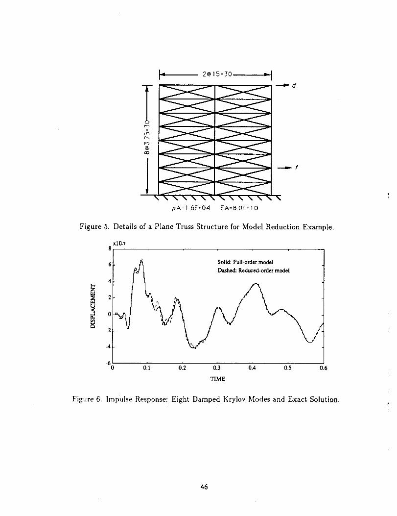
Table 1, from Ref. [14] compares a fixed-interfaceblock-Krylov component-
mode solution and a Craig-Bampton component-mode solution for natural frequen-
cies of the 72 DOF plane truss shown in Fig. 8. The Craig-Bampton method
produces a slightly more accurate reduced model, but at the expense of the addi-
tional computation required to produce the fixed-interface normal modes required by
the Craig-Bampton method.
48
B-K (18 DOF)0.000000E+0O.O00000E+O
0.000000E÷01.953625E-22.205065E-2
4.923845E-2
7.273779E-2
7.626492E-2
1.550032E-1
1.617472E-1
C-B (18 DOF)0.000000E÷0
O.O00000E+OO.O00000E+O1.953688E-2
2.205225E-24.926930E-2
7.231061E-2
7.570881E-2
1.528360E-1
1.586785E-1
FEM (72 DOF)0.000000E+00.000000E+0
0.000000E+01.953624E-2
2.205063E-24.923537E-2
7.229319E-2
7.567759E-2
1.528184E-1
1.586193E-1
Table 1. A Comparison of Block-Krylov and Craig-Bampton Component
Synthesis - Natural Frequencies.
5. Unsymmetric Lanezos Algorithm for Damped Structural Dynamics
Systems (Refs. [12,20,21])
Although most passive damping mechanisms yield a symmetric damping ma-
trix, there are cases when the damping matrix is unsymmetric. For structures, un-
symmetric damping may arise from active feedback control or from Coriolis forces. To
deal with general unsymmetric damping, the usual approach is to write the system's
dynamic equation in first-order state-space form. Then, an unsymmetric Lanczos
algorithm is used to create a basis for model reduction of the first-order differential
equations. References [12,20] describe a two-sided unsymmetric block Lanczos algo-
rithm that generates a set of left Lanczos vectors and a set of right Lanczos vectors
(analogous to sets of left eigenvectors and right eigenvectors). These two sets of
Lanczos vectors form a basis that transforms the system equation to an unsymmetric
block-tridiagonal form. The major disadvantage of a two-sided Lanczos algorithm is
that the reduced-order model that is obtained may exhibit some high-frequency spuri-
ous modes or even unstable modes, although the full-order system is stable. However,
the computational enhancements described in Ref. [12] produce a very robust two-
sided algorithm.
A one-sided Lanczos algorithm for structures with unsymmetric damping ma-
trix and/or stiffness matrix was recently described in Ref. [21]. Consider a linear,
time-invariant system described by Eq. (10). Assume that the system is stable
and completely controllable. Then, the following Lyapunov equation has a unique
positive-definite solution.
AWe + WcA T + BB T = 0 (30)
Wc is called the controllability grammian of the system. If the system's state vector is
49

transformed to another setof coordinates through a nonsingular projection matrix L
z= L5
then the system equation becomes
z = A_,+ [3u
y=C2
where the system matrices in the new coordinates are
7t= L-'AL , [3= L-aB ,
In Ref. [21] the transformation matrix
L=[Q1 Q_ "'" Qk ]
is formed by a three-term Lanczos iteration formula
(31)
AQ, = Qi-l_,-1 + Q,_ - Qi+IG T
(32)
C=CL (33)
(34)
(35)
where
_i-1 = QT-IW[1AQi (36).r, = Qrwi-' AQ_
The Qi's are orthonormalized with respect to the inverse of the controllability gram-
mian of the system. That is
I if i = j (37)QTW_"QJ = 0 if i ¢ j
Then, fit has the almost-skew-symmetric, block-tridiagonal form
(38)
_', g,-6r 7_ 6_
A
Reference [21] lists a complete one-sided, unsymmetric block-Lanczos algorithm
and also discusses special modifications to handle model reduction for unstable sys-
tems, to optimize the choice of starting vectors, to use A-' as the iteration matrix,
and to use the observability grammian instead of the controllability grammian. An
50

force (input)
i 240 cmoutput _ _ _ k
0mEA=2E+2 N p A--2E-2 kg/cm
Figure 9. A Plane Truss Structure.
-4O i , , ,,l,,i , i , , IT
_v
_ -80Z
_-100
. | *)_1 [ l ] l llllll i i i i [llll i i i IiIill i i i }11
To 1 10o 101 10_ 10_
FREQUENCY (Rad/see)
a. Full-order Model vs Twelve-state
Eigenvector-reduced Model.
-4O
_ -60
ctl
_ -80Z
_-100
-12i1 _i
b.
I i i i ilell i e e i g !
I I I I I1111 [ I l|lnll I I I Illlll 1 I Iiirl
10o lOl 102 103
FREQUENCY(P..,_:t/sc_:)
Full-order Model vs Twelve-state
Lanczos-reduced Model with StartingVector B.
Figure 10. Comparison of Frequency Response Functions.
example is provided that utilizes both controllability- and observability-grammian-
based reductions. Figure 9 shows a plane truss structure (16 DOF's; 32 states), and
Figs. 10a,b show frequency response plots of 12-state models based, respectively, on
(complex) eigenvectors and based on (real) Lanczos vectors.
The advantages of the above-described one-sided method over the other exist-
ing unsymmetric Lanczos algorithms are: (1) the numerical breakdown problem that
usually occurs in applying the two-sided unsymmetric Lanczos method is not present,
(2) the Lanczos vectors that are produced lie in the controllable and observable sub-
space, (3) the reduced-order model is guaranteed to be stable, (4) a shifting scheme
can be used for unstable systems, (5) the flexibility of the choice of starting vector can
yield more accurate reduced-order models, and (6) the method is derived for general
multi-input/multi-output systems.
51
6. Krylov/Lanczos Methods for Control of Flexible Structures
Space limitations prevent further discussion in this paper of the application of
Krylov/Lanczos vectors to the control of flexible structures. Several such applications
may be found in Refs. [6,13,22-24].
7. Acknowledgments
This work was supported by NASA Grant NAG9-357 with the NASA Lyndon
B. Johnson Space Center. The authors wish to thank Dr. John Sunkel for his interest
in this work.
References
[1] Parlett, B. N., The Symmetric Eigenvalue Problem, Prentice-Hall, Inc., Engle-
wood Cliffs, N J, 1980.
[2] "Lanczos Method," Section 4.4.3 in MSC NASTRAN Theoretical Manual (Pre-
liminary), Oct. 1985.
[3] Nour-Omid, B. and Clough, R. W., "Dynamic Analysis of Structures Using
Lanczos Coordinates," Earthquake Eng. _ Struc. Dyn., Vol. 12, No. 4, 1984,
pp. 565-577.
[4] Frisch, H. P., IAC Program FEMDA - Theory and User's Guide, NASA Tech
Brief (Draft Copy), June 1989.
[5] Bath_, K. J. and Wilson, E. L., Numerical Methods in Finite Element Analysis,
Prentice-Hall, Inc., Englewood Cliffs, N J, 1976.
[6] Su, T. J., "A Decentralized Linear Quadratic Control Design Method for Flexible
Structures," Ph.D. Dissertation, The University of Texas at Austin, Austin, TX,
Aug. 1989.
[7] Su, T. J. and Craig, R. R. Jr., "Krylov Model Reduction Algorithm for Un-
damped Structural Dynamics Systems," J. Guidance, Control, and Dynamics,
Vol. 14, No. 6, 1991, pp. 1311-1313.
[8] Hickin, J. and Sinha, N. K., "Model Reduction for Linear Multivariable Sys-
tems," IEEE Trans. Automat. Control, Vol. AC-25, No. 6, 1980, pp. 1121-1127.
[9] Villemagne, C. D. and Skelton, R. E., "Model Reduction Using a Projection
Formulation," Int. J. Control, Vot. 46, No. 6, 1987, pp. 2141-2169.
[10] Paige, C. C., "Practical Use of the Symmetric Lanczos Process with Reorthog-
onalization," BIT, Vol. 10, 1970, pp. 183-195.
[11] Parlett, B. N. and Scott, D. S., "The Lanczos Algorithm with Selective Orthog-
onalization," Mathematics of Computation, Vol. 33, No. 145, 1979, pp. 217-238.
52

[12] Kim, H. M. and Craig, R. R. Jr., "Computational Enhancementof an Unsym-
metric Block Lanczos Algorithm," Int. Numer. Methods in Eng., Vol. 30, No. 5,
1990, pp. 1083-1089.
[13] Su, T. J. and Craig, R. R. Jr., "Model Reduction and Control of Flexible Struc-
tures Using Krylov Vectors ," J. Guidance, Control, and Dynamics, Vol. 14,
No. 2, 1991, pp. 260-267.
[14] Craig, R. R. Jr. and Hale, A. L., "The Block-Krylov Component Synthesis
Method for Structural Model Reduction," J. Guidance, Control, and Dynamics,
Vol. 11, No. 6, 1988, pp. 562-570.
[15] Craig, R. R. Jr. and Bampton, M. C. C., "Coupling of Substructures for Dynamic
Analysis," AIAA Journal, Vol. 7, July 1968, pp. 1313-1319.
[16] MacNeal, R. H., "A Hybrid Method of Component Mode Synthesis," Computers
and Structures, Vol. 1, 1971, pp. 581-601.
[17] Rubin, S., "Improved Component-Mode Representation for Structural Dynamic
Analysis," AIAA Journal, Vol. 13, Aug. 1975, pp. 995-1006.
[18] Craig, R. R. Jr. and Chang, C. J., "On the Use of Attachment Modes in Sub-
structure Coupling for Dynamic Analysis," Proceedings of the AIAA 19th Struc-
tures, Structural Dynamics, and Materials Conference, San Diego, CA, 1977, pp.
89-99.
[19] Hurty, W. C., "Dynamic Analysis of Structural Systems Using Component
Modes," AIAA Journal, Vol. 3, April 1965, pp. 678-685.
[20] Kim, H. M. and Craig, R. R. Jr., "Structural Dynamics Analysis Using An
Unsymmetric Block Lanczos Algorithm," Int. J. Numer. Methods in Eng.,
Vol. 26, 1988, pp. 2305-2318.
[21] Su, T. J. and Craig, R. R. Jr., "An Unsymmetric Lanczos Algorithm for Damped
Structural Dynamics Systems," Paper AIAA-92-2510, Proc. AIAA//ASME//
ASCE//AHS//ASC Structures, Structural Dynamics, and Materials Conference,
Dallas, TX, April 1992.
[22] Turner, R. M. and Craig, R. R. Jr., "Use of Lanczos Vectors in Dynamic Sim-
ulation," Report No. CAR86-3, Center for Aeronautical Research, Bureau of
Engineering Research, The University of Texas at Austin, Austin, TX, May1986.
[23] Su, T. J. and Craig, R. R. Jr., "Controller Reduction by Preserving Impulse
Response Energy," AIAA Paper 89-3432, Aug. 1989.
[24] Su, T. J. and Craig, R. R. Jr., "Krylov Vector Methods for Model Reduction and
Control of Flexible Structures," to appear in Advances in Control and Dynamic
Systems.
53

Recommended


![N94-10572 - NASA · N94-10572 PHOTON NUMBER AMPLIFICATION/DUPLICATION ... could produce novel nondassics] ... The Hami]tonian (21)](https://img.pdfslide.net/doc/110x75/5b87fb767f8b9a1a248dff5f/n94-10572-nasa-n94-10572-photon-number-amplificationduplication-could.jpg)