NARMAX-Model-Based Time Series Modeling and
Prediction: Feedforward and Recurrent Fuzzy Neural
Network Approaches
Yang Gao, Member, IEEE and Meng Joo Er, Member, IEEE
School of Electrical and Electronic Engineering
Nanyang Technological University, Singapore
Abstract
The nonlinear autoregressive moving average with exogenous inputs (NARMAX) model provides
a powerful representation for time series analysis, modeling and prediction due to its strength
to accommodate the dynamic, complex and nonlinear nature of real time series applications.
This paper focuses on the modeling and prediction of NARMAX-model-based time series us-
ing the fuzzy neural network (FNN) methodology with an extention of the model represention
include feedforward and recurrent FNNs. This paper introduces and develops a efficient algo-
rithm, namely generalized fuzzy neural network (G-FNN) learning algorithm, for model structure
determination and parameter identification with the aim of producing improved predictive per-
formance for NARMAX time series models. Experiments and comparisons demonstrate that the
proposed G-FNN approaches can effectively learn complex temporal sequences in an adaptive
way and outperform some well-known existing methods.
Keyword
Time series prediction, fuzzy neural networks, NARMAX models.
1
1 Introduction
Time series prediction is an important practical problem with variety of applications in business
and economic planning, inventory and production control, weather forecasting, signal processing,
and many other fields. In the last decade, neural networks (NNs) have been extensively applied
for complex time series processing tasks [3, 4, 8, 9, 10]. This is due to their strength in handling
nonlinear functional dependencies between past time series values and the estimate of the value
to be forecast. More recently, fuzzy logic has been incorporated with the neural models for time
series prediction [1, 2, 5, 6, 11], which are generally known as fuzzy neural networks (FNNs) or
NN-based fuzzy inference systems (FISs) approaches. The FNN possesses both the advantages
of FISs, such as human-like thinking and ease of incorporating expert knowledge, and NNs,
such as learning abilities, optimization abilities and connectionist structures. By virtue of this,
low-level learning and computational power of NNs can be incorporated into the FISs on one
hand and high-level human-like thinking and reasoning of FISs can be incorporated into NNs
on the other hand.
In this paper, NARMAX time series models are investigated using FNN approaches in both
feedforward and recurrent model representations. The proposed FNN predictors have ability
to model complex time series with on-line adjustment, fast learning speed, self-organizing FNN
topology, good generalization and computational efficiency. This is achieved by applying a
sequential and hybrid (supervised/unsupervised) learning algorithm, namely generalized fuzzy
neural network (G-FNN) learning algorithm, to form the FNN prediction model. Various com-
parative analysis are developed to show the advancing performance of the proposed approaches
over some existing methods.
The rest of the paper is organized as follows. Section 2 reviews the NARMAX models as a
point of departure for the use of feedforward and recurrent G-FNNs. The concept of optimal
predictors is also introduced in this section. Section 3 provides a description of the G-FNN
architecture and learning algorithm. In Section 4, one feedforward and two recurrent G-FNN
predictors are proposed for nonlinear time series modeling and prediction. Two experiments
are presented in Section 5 to demonstrate the predictive ability of the proposed methods. The
results are compared with those using a few existing methods. Finally, conclusions and directions
for future research are given in Section 6.
2
2 NARMAX Model and Optimal Predictors
2.1 General NARMAX(ny,ne,nx) Model
The statistical approach for forecasting involves the construction of stochastic models to predict
the value of an observation y(t) using previous observations. A very general class of such models
used for forecasting purpose is the nonlinear autoregressive moving average with exogenous
inputs (NARMAX) models given by
y(t) = F[y(t − 1), . . . , y(t − ny), e(t − 1), . . . , e(t − ne), x(t − 1), . . . , x(t − nx)] + e(t) (1)
where y, e and x are output, noise and external input of the system model respectively, ny, ne
and nx are the maximum lags in the output, noise and input respectively, and F is an unknown
smooth function. It is assumed that e(t) is zero mean, independent and identically distributed,
independent of past y and x, and has a finite variance σ2.
Several special cases of the general NARMAX(ny,ne,nx) model are frequently seen, which
are represented as
NAR(ny) Model:
y(t) = F[y(t − 1), . . . , y(t − ny)] + e(t) (2)
NARMA(ny ,ne) Model:
y(t) = F[y(t − 1), . . . , y(t − ny), e(t − 1), . . . , e(t − ne)] + e(t) (3)
NARX(ny,nx) Model:
y(t) = F[y(t − 1), . . . , y(t − ny), x(t − 1), . . . , x(t − nx)] + e(t) (4)
2.2 Optimal Predictors
Optimum prediction theory focuses on the sense of minimizing mean squared error (MSE). It is
known from [14] that the minimum MSE predictor is the conditional mean as follows, given the
3
infinite past and provided the conditional mean exists.
y(t) = E[y(t)|y(t − 1), y(t − 2), . . .] (5)
In practice, one has only the finite past commencing with the first observation. In this case,
the minimum MSE predictor is [4]
y(t) = E[y(t)|y(t − 1), y(t − 2), . . . , y(1)] (6)
2.2.1 Approximately Optimal NAR(X) Predictors
As it is assumed that e(t) is zero mean and has finite variance σ2 in (1), the optimal predictor
(6) for the NAR(ny) or NARX(ny,nx) model in (2) or (4) is approximately given by
y(t) = E[y(t)|y(t − 1), . . . , y(t − ny)]
= F[y(t − 1), . . . , y(t − ny)] (NAR model) (7)
or
= F[y(t − 1), . . . , y(t − ny), x(t − 1), . . . , x(t − nx)] (NARX model) (8)
where optimal predictors (7) and (8) have MSE σ2.
2.2.2 Approximately Optimal NARMA(X) Predictors
For the NARMA(ny,ne) or NARMAX(ny ,nx,ne) model in (3) or (1), the optimal predictor (6)
is approximately given by
y(t) = E[y(t)|y(t − 1), . . . , y(t − ny)]
= F[y(t − 1), . . . , y(t − ny), e(t − 1), . . . , e(t − ne)] NARMA model (9)
or
= F[y(t − 1), . . . , y(t − ny), e(t − 1), . . . , e(t − ne), x(t − 1), . . . , x(t − nx)]
NARMAX model (10)
where e = y − y.
4
In this case, the following initial conditions are often used
y(t) = e(t) = 0 t ≤ 0 (11)
3 Basic G-FNN = Takagi-Sugeno-Kan-Type FIS
In this section, basic G-FNN architecture and learning algorithm are introduced as the prelimi-
nary knowledge for FNN predictor designs in the next section.
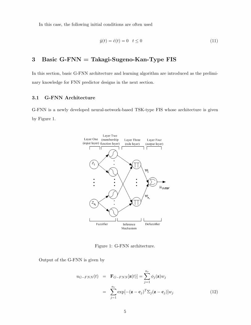
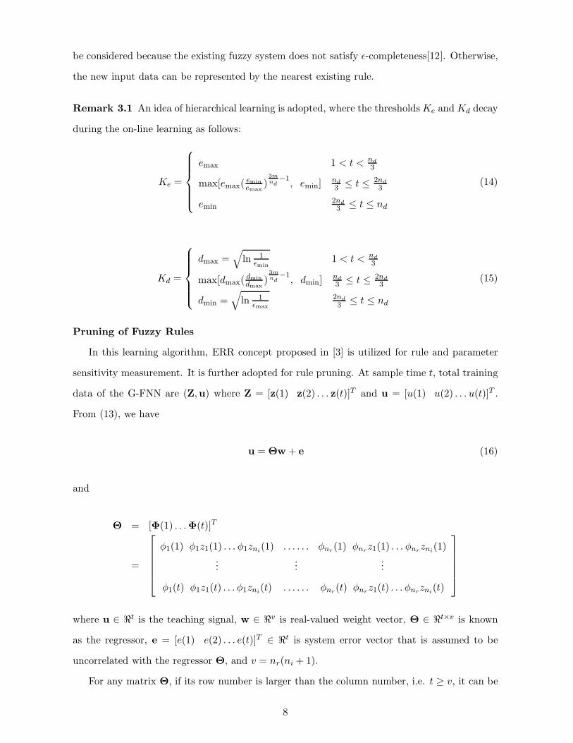
3.1 G-FNN Architecture
G-FNN is a newly developed neural-network-based TSK-type FIS whose architecture is given
by Figure 1.
Figure 1: G-FNN architecture.
Output of the G-FNN is given by
uG−FNN(t) = FG−FNN [z(t)] =nr∑
j=1
φj(z)wj
=nr∑j=1
exp[−(z − cj)T Σj(z − cj)]wj (12)
5
where input vector z = [z1 . . . zni ]T , center vector cj = [c1j . . . cnij]
T and width matrix Σj =
diag( 1σ21j
. . . 1σ2
nij) for Gaussian membership function of jth rule, TSK-type weight vector wj =
k0j + k1jz1 + . . . + knijzni of jth rule, and kijs are real-valued parameters.
Eq. (12) can be represented in matrix form as
uG−FNN (t) = ΦT (t)w (13)
where regression vector Φ = [φ1 φ1z1 . . . φ1zni . . . . . . φnr φnrz1 . . . φnrzni ]T and weight vector
w = [k01 k11 . . . kni1 . . . . . . k0nr k1nr . . . kninr ]T
3.2 G-FNN Learning Algorithm
In this paper, structure and parameters of the time series model is formed automatically and
dynamically using G-FNN learning algorithm. The G-FNN learning algorithm is a sequential
and hybrid (supervised/unsupervised) learning algorithm, which provides an efficient way to
construct the G-FNN model online and combine structure and parameter learning simultane-
ously within the G-FNN. The structure learning includes determining the proper number of
membership function nr, i.e. the coarse of input fuzzy partitions and the finding of correct
fuzzy logic rules. The learning of network parameters corresponds to the learning of the premise
and consequent parameters of the G-FNN. Premise parameters include membership function
parameters cj and Σj, and consequent parameter refers to the weight wj of the G-FNN.
Parameter learning is performed by combining the semi-closed fuzzy set concept for the
membership learning and the linear least square (LLS) method for weight learning. For structure
learning, two criteria are proposed for fuzzy rule generation and an error reduction ratio (ERR)
concept is proposed for rule pruning. Given the supervised training data, the proposed learning
algorithm first decides whether or not to perform the fuzzy rule generation based on two proposed
criteria. If structure learning is necessary, premise parameters of a new fuzzy rule will be obtained
using semi-closed fuzzy set concept. The G-FNN will further decide whether there are redundant
rules to be deleted based on the ERR, and it will also change the consequences of all the fuzzy
rules properly. If no structure learning is necessary, the parameter learning will be performed to
adjust the current premise and consequent parameters. This structure/parameter learning will
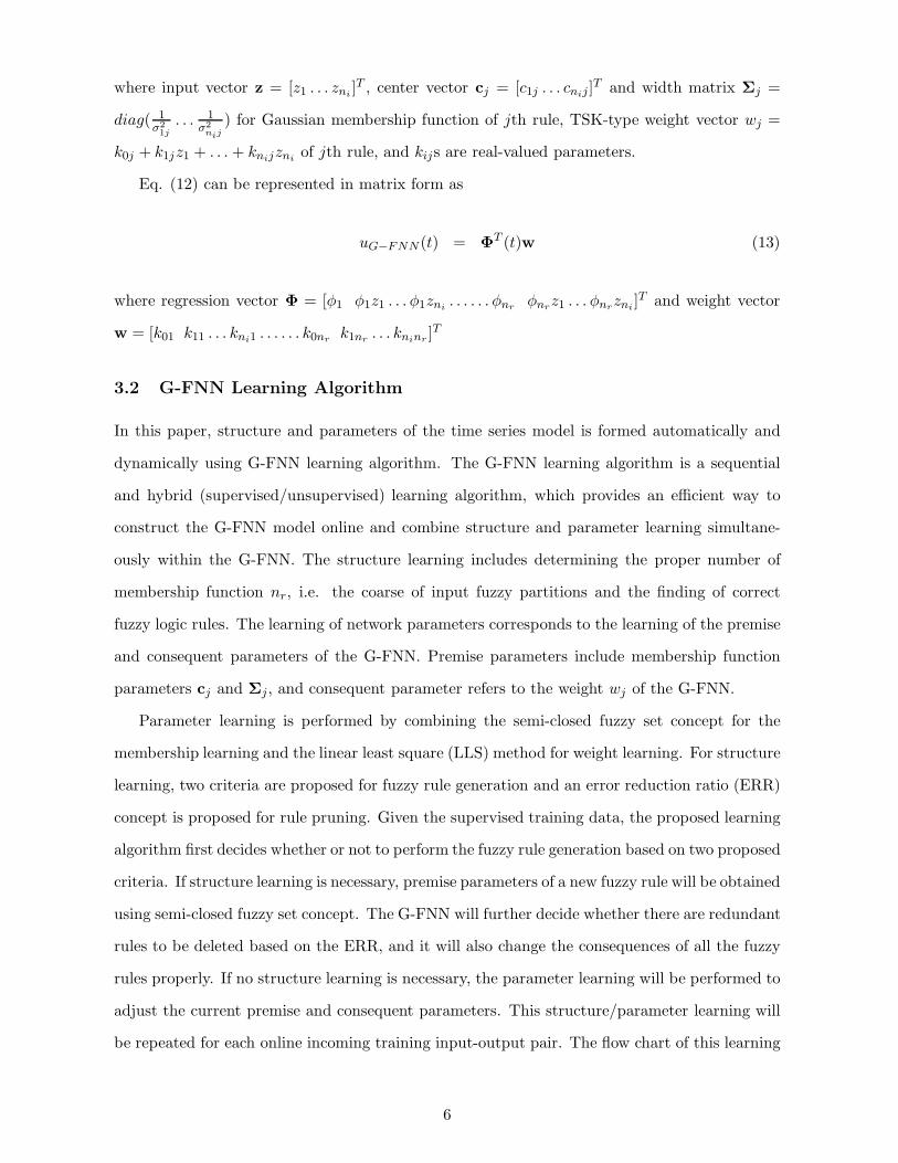
be repeated for each online incoming training input-output pair. The flow chart of this learning
6
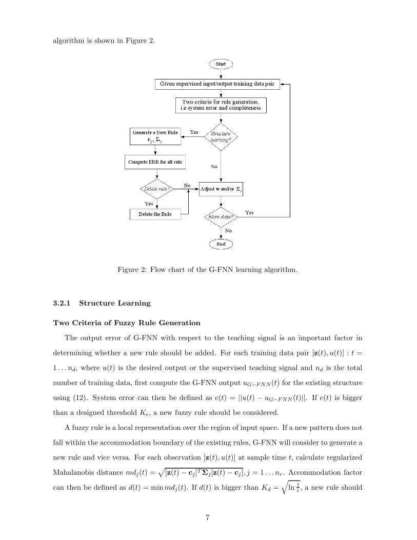
algorithm is shown in Figure 2.
Figure 2: Flow chart of the G-FNN learning algorithm.
3.2.1 Structure Learning
Two Criteria of Fuzzy Rule Generation
The output error of G-FNN with respect to the teaching signal is an important factor in
determining whether a new rule should be added. For each training data pair [z(t), u(t)] : t =
1 . . . nd, where u(t) is the desired output or the supervised teaching signal and nd is the total
number of training data, first compute the G-FNN output uG−FNN(t) for the existing structure
using (12). System error can then be defined as e(t) = ||u(t) − uG−FNN (t)||. If e(t) is bigger
than a designed threshold Ke, a new fuzzy rule should be considered.
A fuzzy rule is a local representation over the region of input space. If a new pattern does not
fall within the accommodation boundary of the existing rules, G-FNN will consider to generate a
new rule and vice versa. For each observation [z(t), u(t)] at sample time t, calculate regularized
Mahalanobis distance mdj(t) =√
[z(t) − cj ]TΣj[z(t) − cj ], j = 1 . . . nr. Accommodation factor
can then be defined as d(t) = minmdj(t). If d(t) is bigger than Kd =√
ln 1ε , a new rule should
7
be considered because the existing fuzzy system does not satisfy ε-completeness[12]. Otherwise,
the new input data can be represented by the nearest existing rule.
Remark 3.1 An idea of hierarchical learning is adopted, where the thresholds Ke and Kd decay
during the on-line learning as follows:
Ke =
emax 1 < t < nd3
max[emax( eminemax
)3mnd
−1, emin] nd
3 ≤ t ≤ 2nd3
emin2nd3 ≤ t ≤ nd
(14)
Kd =
dmax =√
ln 1εmin
1 < t < nd3
max[dmax( dmindmax
)3mnd
−1, dmin] nd
3 ≤ t ≤ 2nd3
dmin =√
ln 1εmax
2nd3 ≤ t ≤ nd
(15)
Pruning of Fuzzy Rules
In this learning algorithm, ERR concept proposed in [3] is utilized for rule and parameter
sensitivity measurement. It is further adopted for rule pruning. At sample time t, total training
data of the G-FNN are (Z,u) where Z = [z(1) z(2) . . . z(t)]T and u = [u(1) u(2) . . . u(t)]T .
From (13), we have
u = Θw + e (16)
and
Θ = [Φ(1) . . . Φ(t)]T
=
φ1(1) φ1z1(1) . . . φ1zni(1) . . . . . . φnr(1) φnrz1(1) . . . φnrzni(1)...
......
φ1(t) φ1z1(t) . . . φ1zni(t) . . . . . . φnr(t) φnrz1(t) . . . φnrzni(t)
where u ∈ �t is the teaching signal, w ∈ �v is real-valued weight vector, Θ ∈ �t×v is known
as the regressor, e = [e(1) e(2) . . . e(t)]T ∈ �t is system error vector that is assumed to be
uncorrelated with the regressor Θ, and v = nr(ni + 1).
For any matrix Θ, if its row number is larger than the column number, i.e. t ≥ v, it can be
8
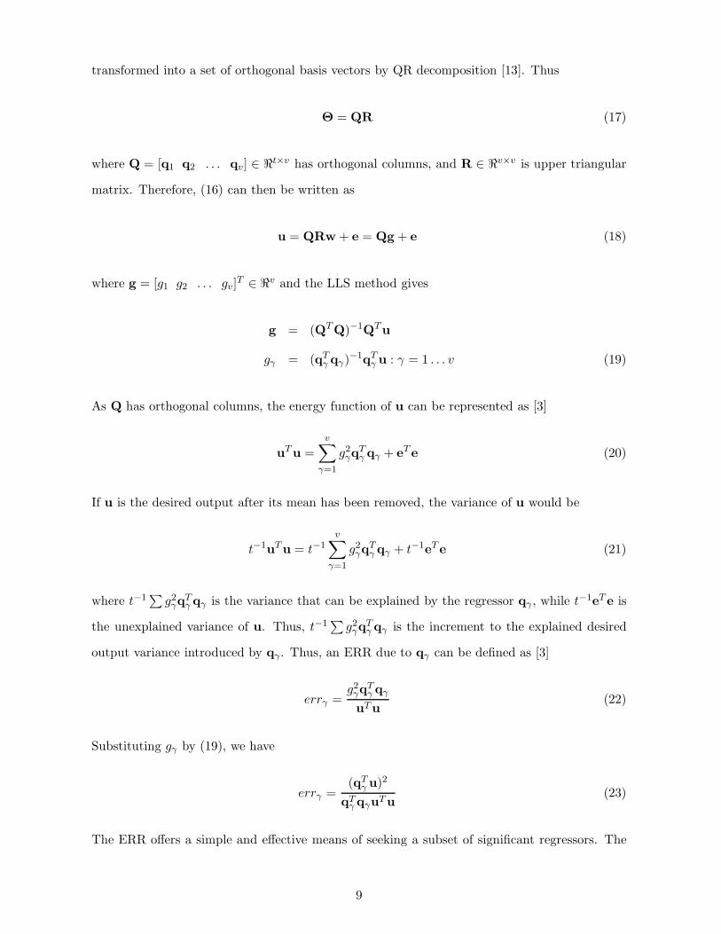
transformed into a set of orthogonal basis vectors by QR decomposition [13]. Thus
Θ = QR (17)
where Q = [q1 q2 . . . qv] ∈ �t×v has orthogonal columns, and R ∈ �v×v is upper triangular
matrix. Therefore, (16) can then be written as
u = QRw + e = Qg + e (18)
where g = [g1 g2 . . . gv]T ∈ �v and the LLS method gives
g = (QTQ)−1QTu
gγ = (qTγ qγ)−1qT
γ u : γ = 1 . . . v (19)
As Q has orthogonal columns, the energy function of u can be represented as [3]
uTu =v∑
γ=1
g2γq
Tγ qγ + eTe (20)
If u is the desired output after its mean has been removed, the variance of u would be
t−1uTu = t−1v∑
γ=1
g2γq
Tγ qγ + t−1eTe (21)
where t−1∑
g2γq
Tγ qγ is the variance that can be explained by the regressor qγ , while t−1eTe is
the unexplained variance of u. Thus, t−1∑
g2γq
Tγ qγ is the increment to the explained desired
output variance introduced by qγ . Thus, an ERR due to qγ can be defined as [3]
errγ =g2γq
Tγ qγ
uTu(22)
Substituting gγ by (19), we have
errγ =(qT
γ u)2
qTγ qγuTu
(23)
The ERR offers a simple and effective means of seeking a subset of significant regressors. The
9
term errγ in (23) reflects the similarity of qγ and u or the inner product of qγ and u. Larger
errγ implies that qγ is more significant to the output u.
The ERR matrix of the G-FNN is defined as
ERR =
err1 err2 . . . errnr
errnr+1 errnr+2 . . . errnr+nr
...... . . .
...
errni×nr+1 errni×nr+2 . . . errni×nr+nr
(24)
=[
err1 err2 . . . errnr
](25)
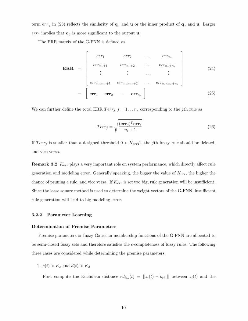
We can further define the total ERR Terrj, j = 1 . . . nr corresponding to the jth rule as
Terrj =
√(errj)Terrj
ni + 1(26)
If Terrj is smaller than a designed threshold 0 < Kerr¡1, the jth fuzzy rule should be deleted,
and vice versa.
Remark 3.2 Kerr plays a very important role on system performance, which directly affect rule
generation and modeling error. Generally speaking, the bigger the value of Kerr, the higher the
chance of pruning a rule, and vice versa. If Kerr is set too big, rule generation will be insufficient.
Since the lease square method is used to determine the weight vectors of the G-FNN, insufficient
rule generation will lead to big modeling error.
3.2.2 Parameter Learning
Determination of Premise Parameters
Premise parameters or fuzzy Gaussian membership functions of the G-FNN are allocated to
be semi-closed fuzzy sets and therefore satisfies the ε-completeness of fuzzy rules. The following
three cases are considered while determining the premise parameters:
1. e(t) > Ke and d(t) > Kd
First compute the Euclidean distance edijn(t) = ||zi(t) − bijn || between zi(t) and the
10
boundary point bijn ∈ {ci1, ci2, . . . , ciNr , zi,min, zi,max}. Find
jn = arg min edijn(t) (27)
If edijn(t) is less than a threshold or a dissimilarity ratio of neighboring membership
function Kmf , we choose
ci(nr+1) = bijn, σi(nr+1) = σijn
(28)
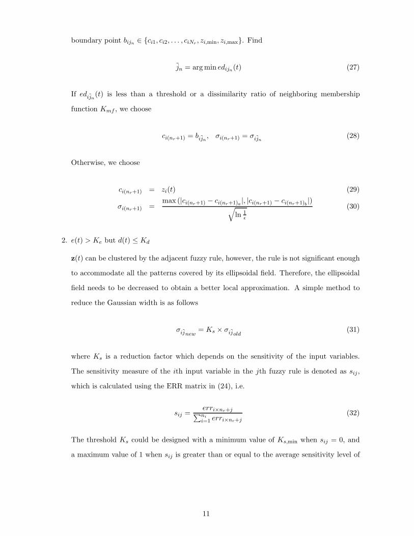
Otherwise, we choose
ci(nr+1) = zi(t) (29)
σi(nr+1) =max (|ci(nr+1) − ci(nr+1)a
|, |ci(nr+1) − ci(nr+1)b|)√
ln 1ε
(30)
2. e(t) > Ke but d(t) ≤ Kd
z(t) can be clustered by the adjacent fuzzy rule, however, the rule is not significant enough
to accommodate all the patterns covered by its ellipsoidal field. Therefore, the ellipsoidal
field needs to be decreased to obtain a better local approximation. A simple method to
reduce the Gaussian width is as follows
σijnew= Ks × σijold
(31)
where Ks is a reduction factor which depends on the sensitivity of the input variables.
The sensitivity measure of the ith input variable in the jth fuzzy rule is denoted as sij ,
which is calculated using the ERR matrix in (24), i.e.
sij =erri×nr+j∑nii=1 erri×nr+j
(32)
The threshold Ks could be designed with a minimum value of Ks,min when sij = 0, and
a maximum value of 1 when sij is greater than or equal to the average sensitivity level of
11
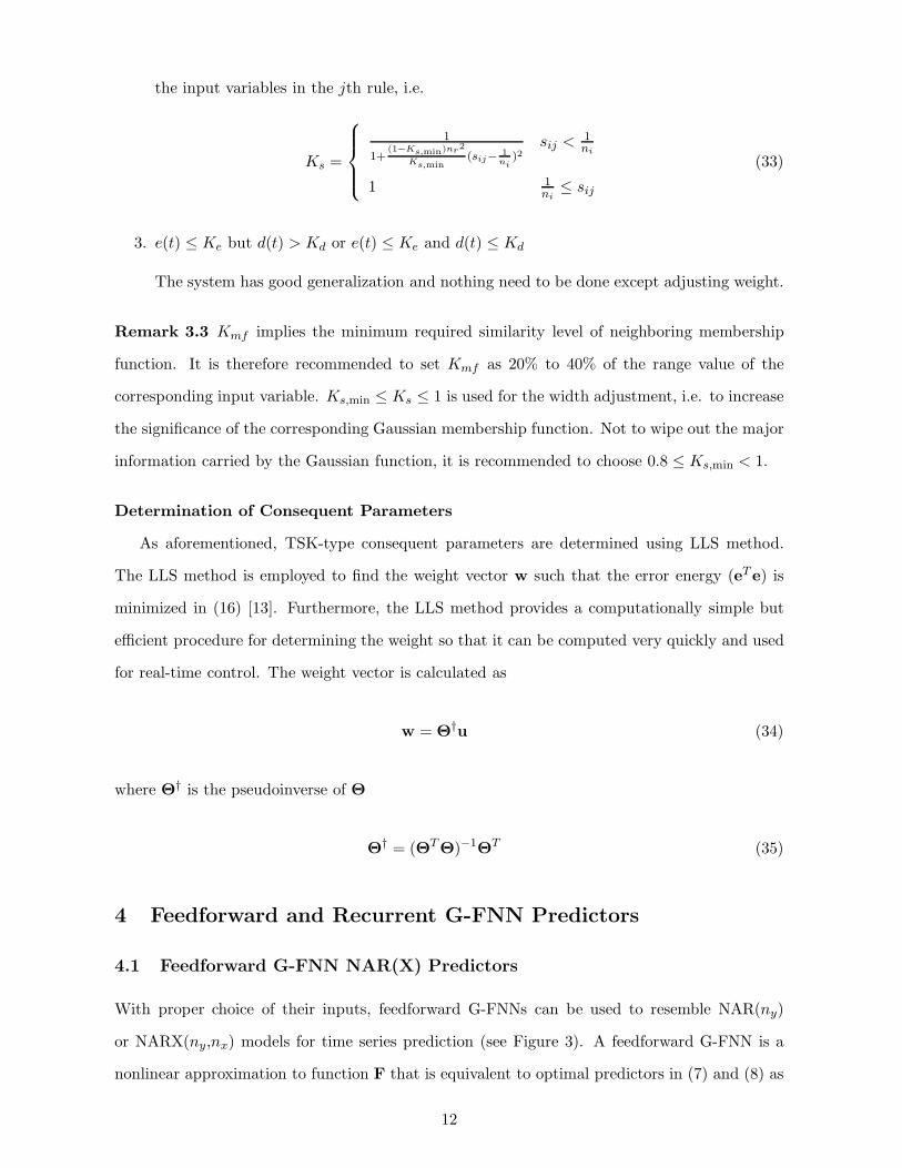
the input variables in the jth rule, i.e.
Ks =
1
1+(1−Ks,min)nr2
Ks,min(sij− 1
ni)2
sij < 1ni
1 1ni
≤ sij
(33)
3. e(t) ≤ Ke but d(t) > Kd or e(t) ≤ Ke and d(t) ≤ Kd
The system has good generalization and nothing need to be done except adjusting weight.
Remark 3.3 Kmf implies the minimum required similarity level of neighboring membership
function. It is therefore recommended to set Kmf as 20% to 40% of the range value of the
corresponding input variable. Ks,min ≤ Ks ≤ 1 is used for the width adjustment, i.e. to increase
the significance of the corresponding Gaussian membership function. Not to wipe out the major
information carried by the Gaussian function, it is recommended to choose 0.8 ≤ Ks,min < 1.
Determination of Consequent Parameters
As aforementioned, TSK-type consequent parameters are determined using LLS method.
The LLS method is employed to find the weight vector w such that the error energy (eTe) is
minimized in (16) [13]. Furthermore, the LLS method provides a computationally simple but
efficient procedure for determining the weight so that it can be computed very quickly and used
for real-time control. The weight vector is calculated as
w = Θ†u (34)
where Θ† is the pseudoinverse of Θ
Θ† = (ΘT Θ)−1ΘT (35)
4 Feedforward and Recurrent G-FNN Predictors
4.1 Feedforward G-FNN NAR(X) Predictors
With proper choice of their inputs, feedforward G-FNNs can be used to resemble NAR(ny)
or NARX(ny,nx) models for time series prediction (see Figure 3). A feedforward G-FNN is a
nonlinear approximation to function F that is equivalent to optimal predictors in (7) and (8) as
12
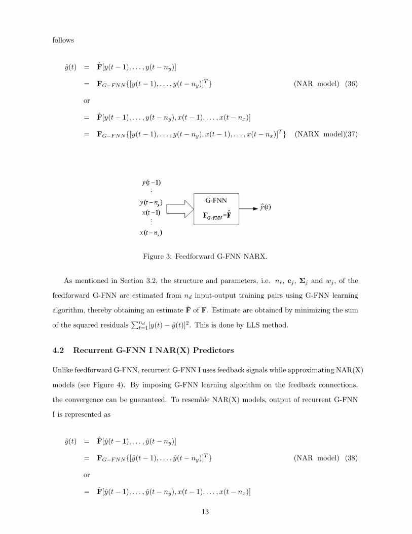
follows
y(t) = F[y(t − 1), . . . , y(t − ny)]
= FG−FNN{[y(t − 1), . . . , y(t − ny)]T } (NAR model) (36)
or
= F[y(t − 1), . . . , y(t − ny), x(t − 1), . . . , x(t − nx)]
= FG−FNN{[y(t − 1), . . . , y(t − ny), x(t − 1), . . . , x(t − nx)]T } (NARX model)(37)
Figure 3: Feedforward G-FNN NARX.
As mentioned in Section 3.2, the structure and parameters, i.e. nr, cj , Σj and wj , of the
feedforward G-FNN are estimated from nd input-output training pairs using G-FNN learning
algorithm, thereby obtaining an estimate F of F. Estimate are obtained by minimizing the sum
of the squared residuals∑nd
t=1[y(t) − y(t)]2. This is done by LLS method.
4.2 Recurrent G-FNN I NAR(X) Predictors
Unlike feedforward G-FNN, recurrent G-FNN I uses feedback signals while approximating NAR(X)
models (see Figure 4). By imposing G-FNN learning algorithm on the feedback connections,
the convergence can be guaranteed. To resemble NAR(X) models, output of recurrent G-FNN
I is represented as
y(t) = F[y(t − 1), . . . , y(t − ny)]
= FG−FNN{[y(t − 1), . . . , y(t − ny)]T } (NAR model) (38)
or
= F[y(t − 1), . . . , y(t − ny), x(t − 1), . . . , x(t − nx)]
13
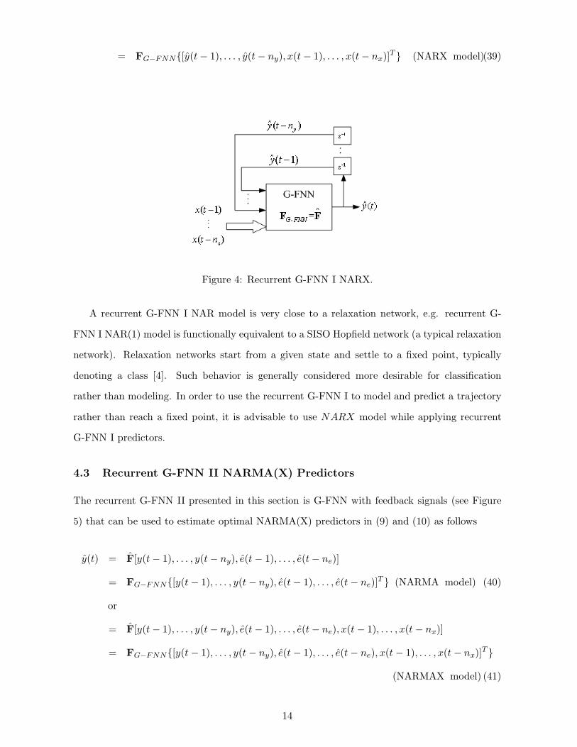
= FG−FNN{[y(t − 1), . . . , y(t − ny), x(t − 1), . . . , x(t − nx)]T } (NARX model)(39)
Figure 4: Recurrent G-FNN I NARX.
A recurrent G-FNN I NAR model is very close to a relaxation network, e.g. recurrent G-
FNN I NAR(1) model is functionally equivalent to a SISO Hopfield network (a typical relaxation
network). Relaxation networks start from a given state and settle to a fixed point, typically
denoting a class [4]. Such behavior is generally considered more desirable for classification
rather than modeling. In order to use the recurrent G-FNN I to model and predict a trajectory
rather than reach a fixed point, it is advisable to use NARX model while applying recurrent
G-FNN I predictors.
4.3 Recurrent G-FNN II NARMA(X) Predictors
The recurrent G-FNN II presented in this section is G-FNN with feedback signals (see Figure
5) that can be used to estimate optimal NARMA(X) predictors in (9) and (10) as follows
y(t) = F[y(t − 1), . . . , y(t − ny), e(t − 1), . . . , e(t − ne)]
= FG−FNN{[y(t − 1), . . . , y(t − ny), e(t − 1), . . . , e(t − ne)]T } (NARMA model) (40)
or
= F[y(t − 1), . . . , y(t − ny), e(t − 1), . . . , e(t − ne), x(t − 1), . . . , x(t − nx)]
= FG−FNN{[y(t − 1), . . . , y(t − ny), e(t − 1), . . . , e(t − ne), x(t − 1), . . . , x(t − nx)]T }
(NARMAX model) (41)
14
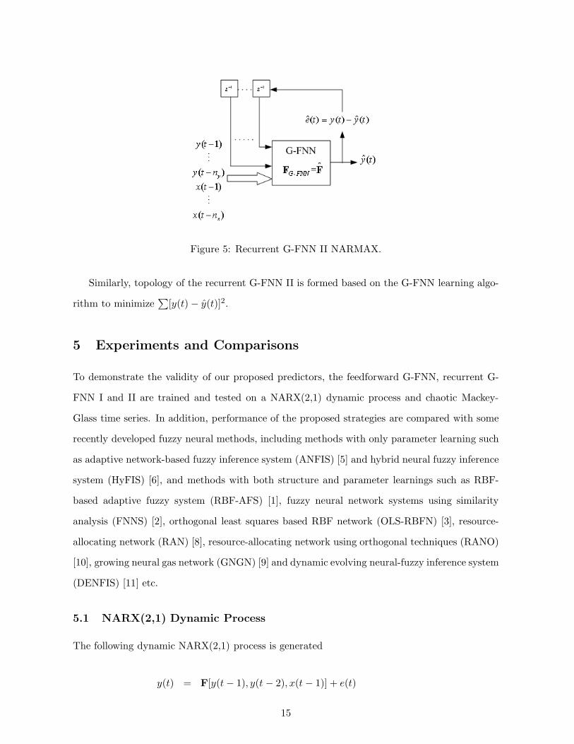
Figure 5: Recurrent G-FNN II NARMAX.
Similarly, topology of the recurrent G-FNN II is formed based on the G-FNN learning algo-
rithm to minimize∑
[y(t) − y(t)]2.
5 Experiments and Comparisons
To demonstrate the validity of our proposed predictors, the feedforward G-FNN, recurrent G-
FNN I and II are trained and tested on a NARX(2,1) dynamic process and chaotic Mackey-
Glass time series. In addition, performance of the proposed strategies are compared with some
recently developed fuzzy neural methods, including methods with only parameter learning such
as adaptive network-based fuzzy inference system (ANFIS) [5] and hybrid neural fuzzy inference
system (HyFIS) [6], and methods with both structure and parameter learnings such as RBF-
based adaptive fuzzy system (RBF-AFS) [1], fuzzy neural network systems using similarity
analysis (FNNS) [2], orthogonal least squares based RBF network (OLS-RBFN) [3], resource-
allocating network (RAN) [8], resource-allocating network using orthogonal techniques (RANO)
[10], growing neural gas network (GNGN) [9] and dynamic evolving neural-fuzzy inference system
(DENFIS) [11] etc.
5.1 NARX(2,1) Dynamic Process
The following dynamic NARX(2,1) process is generated
y(t) = F[y(t − 1), y(t − 2), x(t − 1)] + e(t)
15
=y(t − 1)y(t − 2)[y(t − 1) + 2.5]
1 + y2(t − 1) + y2(t − 2)+ x(t − 1) + e(t) (42)
where the input has the form x(t) = sin(2πt/25). In this example, thresholds of the G-FNN
learning algorithm are predefined in a systematic manner based on the desired accuracy level of
the system (refer to Appendix), i.e. emax = 0.1, emin = 0.02, dmax =√
ln( 10.5), dmin =
√ln( 1
0.8),
Ks,min = 0.9, Kmf = 0.5 and Kerr = 0.002. The topology of all feedforward and recurrent G-
FNNs are estimated using the first 200 observations of a time series generated from NARX(2,1)
model in (42). The feedforward and recurrent G-FNN predictors are then tested on the following
200 observations from the model.
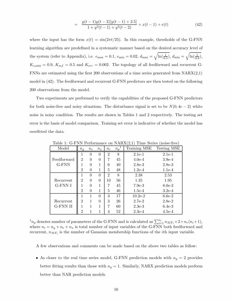
Two experiments are performed to verify the capabilities of the proposed G-FNN predictors
for both noise-free and noisy situations. The disturbance signal is set to be N(0, 4e − 2) white
noise in noisy condition. The results are shown in Tables 1 and 2 respectively. The testing set
error is the basis of model comparison. Training set error is indicative of whether the model has
overfitted the data.
Table 1: G-FNN Performance on NARX(2,1) Time Series (noise-free)Model ny ne nx nr np
1 Training MSE Testing MSE1 0 0 2 8 2.1e-1 2.1e-1
Feedforward 2 0 0 7 45 4.0e-4 3.9e-4G-FNN 1 0 1 6 40 2.8e-3 2.8e-3
2 0 1 5 48 1.2e-4 1.1e-41 0 0 2 8 2.38 2.53
Recurrent 2 0 0 10 56 1.35 1.95G-FNN I 1 0 1 7 45 7.9e-3 8.0e-3
2 0 1 5 46 1.5e-4 3.2e-41 1 0 3 17 10.2e-2 6.6e-2
Recurrent 2 1 0 3 26 2.7e-2 2.8e-2G-FNN II 1 1 1 7 60 2.3e-3 6.4e-3
2 1 1 4 52 2.3e-4 4.5e-4
1np denotes number of parameters of the G-FNN and is calculated as∑ni
i=1 nMFi ×2+nr(ni+1),where ni = ny + ne + nx is total number of input variables of the G-FNN both feedforward andrecurrent, nMFi is the number of Gaussian membership functions of the ith input variable.
A few observations and comments can be made based on the above two tables as follow:
• As closer to the real time series model, G-FNN prediction models with ny = 2 provides
better fitting results than those with ny = 1. Similarly, NARX prediction models perform
better than NAR prediction models.
16
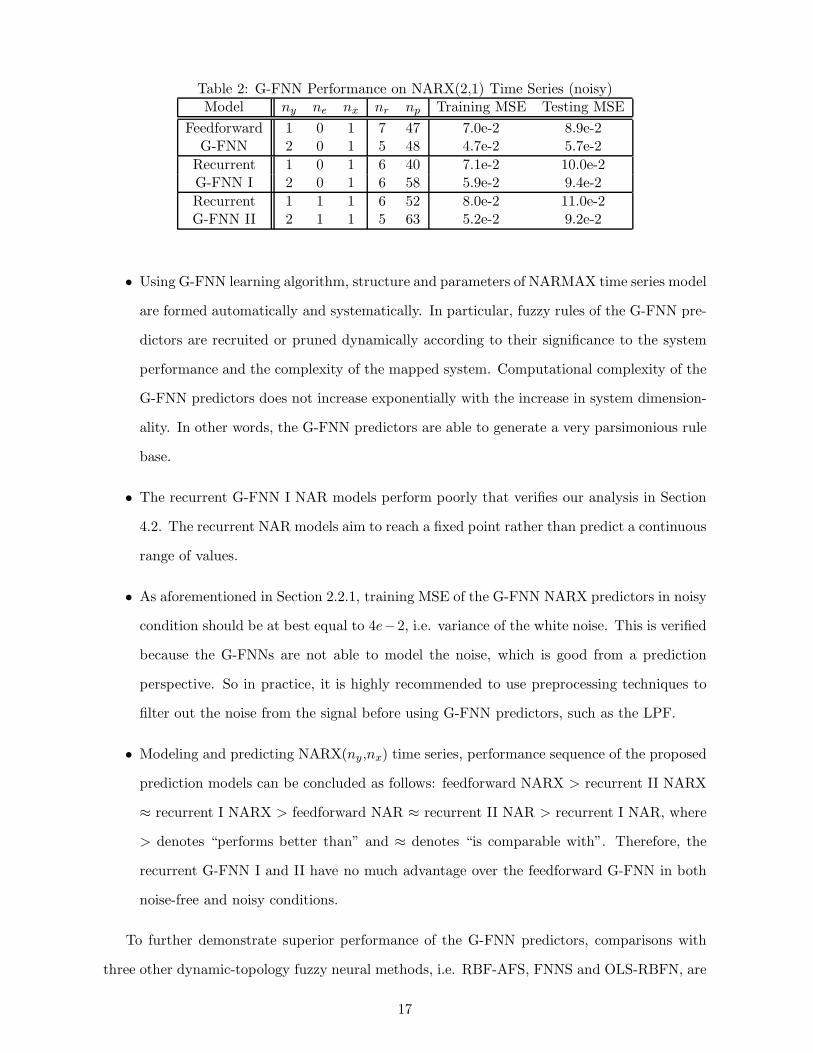
Table 2: G-FNN Performance on NARX(2,1) Time Series (noisy)Model ny ne nx nr np Training MSE Testing MSE
Feedforward 1 0 1 7 47 7.0e-2 8.9e-2G-FNN 2 0 1 5 48 4.7e-2 5.7e-2
Recurrent 1 0 1 6 40 7.1e-2 10.0e-2G-FNN I 2 0 1 6 58 5.9e-2 9.4e-2Recurrent 1 1 1 6 52 8.0e-2 11.0e-2G-FNN II 2 1 1 5 63 5.2e-2 9.2e-2
• Using G-FNN learning algorithm, structure and parameters of NARMAX time series model
are formed automatically and systematically. In particular, fuzzy rules of the G-FNN pre-
dictors are recruited or pruned dynamically according to their significance to the system
performance and the complexity of the mapped system. Computational complexity of the
G-FNN predictors does not increase exponentially with the increase in system dimension-
ality. In other words, the G-FNN predictors are able to generate a very parsimonious rule
base.
• The recurrent G-FNN I NAR models perform poorly that verifies our analysis in Section
4.2. The recurrent NAR models aim to reach a fixed point rather than predict a continuous
range of values.
• As aforementioned in Section 2.2.1, training MSE of the G-FNN NARX predictors in noisy
condition should be at best equal to 4e−2, i.e. variance of the white noise. This is verified
because the G-FNNs are not able to model the noise, which is good from a prediction
perspective. So in practice, it is highly recommended to use preprocessing techniques to
filter out the noise from the signal before using G-FNN predictors, such as the LPF.
• Modeling and predicting NARX(ny,nx) time series, performance sequence of the proposed
prediction models can be concluded as follows: feedforward NARX > recurrent II NARX
≈ recurrent I NARX > feedforward NAR ≈ recurrent II NAR > recurrent I NAR, where
> denotes “performs better than” and ≈ denotes “is comparable with”. Therefore, the
recurrent G-FNN I and II have no much advantage over the feedforward G-FNN in both
noise-free and noisy conditions.
To further demonstrate superior performance of the G-FNN predictors, comparisons with
three other dynamic-topology fuzzy neural methods, i.e. RBF-AFS, FNNS and OLS-RBFN, are
17
shown in Table 3. In this comparison, noise-free signal and fitting model with ny = 2 and nx = 1
are used for all the methods. It can be seen that the G-FNN provides better generalization as
well as greater parsimony. The proposed G-FNN predictors are fast in learning speed because
no iterative learning loops are needed. Generating less number of rules and parameters leads to
better computational efficiency using G-FNN learning algorithm.
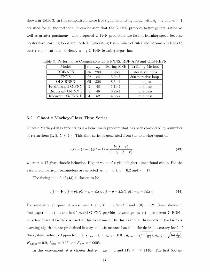
Table 3: Performance Comparisons with FNNS, RBF-AFS and OLS-RBFNModel nr np Testing MSE Training Method
RBF-AFS 35 280 1.9e-2 iterative loopsFNNS 22 84 5.0e-3 300 iterative loops
OLS-RBFN 65 326 8.3e-4 one passFeedforward G-FNN 5 48 1.1e-4 one passRecurrent G-FNN I 5 46 3.2e-4 one passRecurrent G-FNN II 4 52 4.5e-4 one pass
5.2 Chaotic Mackey-Glass Time Series
Chaotic Mackey-Glass time series is a benchmark problem that has been considered by a number
of researchers [1, 3, 5, 8, 10]. This time series is generated from the following equation
y(t) = (1 − a)y(t − 1) +by(t − τ)
1 + y10(t − τ)(43)
where τ > 17 gives chaotic behavior. Higher value of τ yields higher dimensional chaos. For the
ease of comparison, parameters are selected as: a = 0.1, b = 0.2 and τ = 17.
The fitting model of (43) is chosen to be
y(t) = F[y(t − p), y(t − p −�t), y(t − p − 2�t), y(t − p − 3�t)] (44)
For simulation purpose, it is assumed that y(t) = 0, ∀t < 0 and y(0) = 1.2. Since shown in
first experiment that the feedforward G-FNN provides advantages over the recurrent G-FNNs,
only feedforward G-FNN is used in this experiment. In this example, thresholds of the G-FNN
learning algorithm are predefined in a systematic manner based on the desired accuracy level of
the system (refer to Appendix), i.e. emax = 0.1, emin = 0.01, dmax =√
ln( 10.5), dmin =
√ln( 1
0.8),
Ks,min = 0.9, Kmf = 0.25 and Kerr = 0.0005.
In this experiment, it is chosen that p = �t = 6 and 119 ≤ t ≤ 1140. The first 500 in-
18
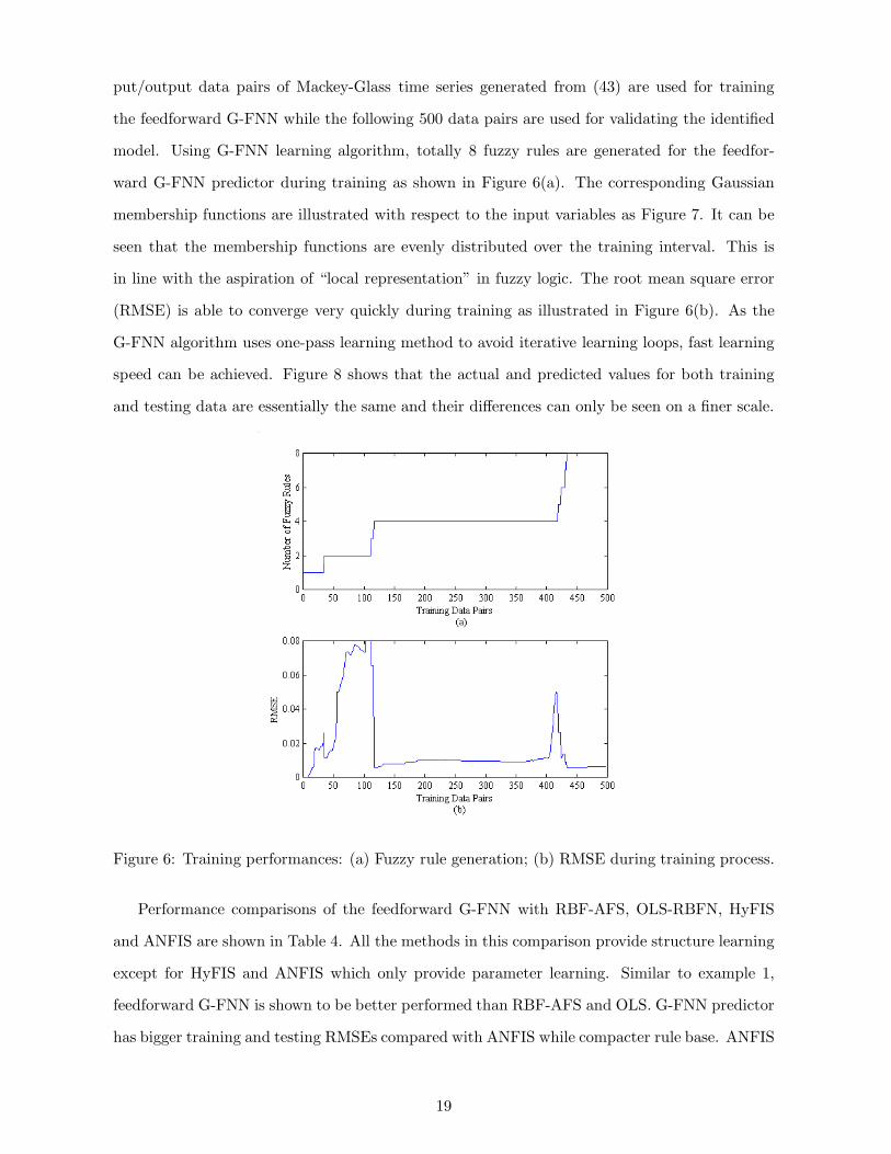
put/output data pairs of Mackey-Glass time series generated from (43) are used for training
the feedforward G-FNN while the following 500 data pairs are used for validating the identified
model. Using G-FNN learning algorithm, totally 8 fuzzy rules are generated for the feedfor-
ward G-FNN predictor during training as shown in Figure 6(a). The corresponding Gaussian
membership functions are illustrated with respect to the input variables as Figure 7. It can be
seen that the membership functions are evenly distributed over the training interval. This is
in line with the aspiration of “local representation” in fuzzy logic. The root mean square error
(RMSE) is able to converge very quickly during training as illustrated in Figure 6(b). As the
G-FNN algorithm uses one-pass learning method to avoid iterative learning loops, fast learning
speed can be achieved. Figure 8 shows that the actual and predicted values for both training
and testing data are essentially the same and their differences can only be seen on a finer scale.
Figure 6: Training performances: (a) Fuzzy rule generation; (b) RMSE during training process.
Performance comparisons of the feedforward G-FNN with RBF-AFS, OLS-RBFN, HyFIS
and ANFIS are shown in Table 4. All the methods in this comparison provide structure learning
except for HyFIS and ANFIS which only provide parameter learning. Similar to example 1,
feedforward G-FNN is shown to be better performed than RBF-AFS and OLS. G-FNN predictor
has bigger training and testing RMSEs compared with ANFIS while compacter rule base. ANFIS
19
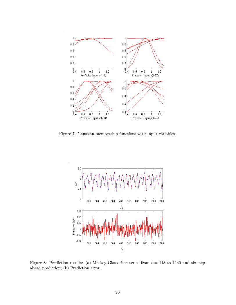
Figure 7: Gaussian membership functions w.r.t input variables.
Figure 8: Prediction results: (a) Mackey-Glass time series from t = 118 to 1140 and six-stepahead prediction; (b) Prediction error.
20
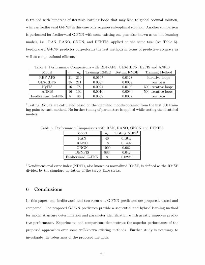
is trained with hundreds of iterative learning loops that may lead to global optimal solution,
whereas feedforward G-FNN in this case only acquires sub-optimal solution. Another comparison
is performed for feedforward G-FNN with some existing one-pass also known as on-line learning
models, i.e. RAN, RANO, GNGN, and DENFIS, applied on the same task (see Table 5).
Feedforward G-FNN predictor outperforms the rest methods in terms of predictive accuracy as
well as computational efficency.
Table 4: Performance Comparisons with RBF-AFS, OLS-RBFN, HyFIS and ANFISModel nr np Training RMSE Testing RMSE1 Training Method
RBF-AFS 21 210 0.0107 0.0128 iterative loopsOLS-RBFN 35 211 0.0087 0.0089 one pass
HyFIS 16 78 0.0021 0.0100 500 iterative loopsANFIS 16 104 0.0016 0.0030 500 iterative loops
Feedforward G-FNN 8 86 0.0062 0.0052 one pass
1Testing RMSEs are calculated based on the identified models obtained from the first 500 train-ing pairs by each method. No further tuning of parameters is applied while testing the identifiedmodels.
Table 5: Performance Comparisons with RAN, RANO, GNGN and DENFISModel nr Testing NDEI1
RAN 40 0.1642RANO 18 0.1492GNGN 1000 0.062
DENFIS 883 0.042Feedforward G-FNN 8 0.0226
1Nondimensional error index (NDEI), also known as normalized RMSE, is defined as the RMSEdivided by the standard deviation of the target time series.
6 Conclusions
In this paper, one feedforward and two recurrent G-FNN predictors are proposed, tested and
compared. The proposed G-FNN predictors provide a sequential and hybrid learning method
for model structure determination and parameter identification which greatly improves predic-
tive performance. Experiments and comparisons demonstrate the superior performance of the
proposed approaches over some well-known existing methods. Further study is necessary to
investigate the robustness of the proposed methods.
21
References
[1] K. B. Cho and B. H. Wang, “Radial Basis Function Based Adaptive Fuzzy Systems and
their Applications to System Identification and Prediction,” Fuzzy Sets and Systems, Vol.
83, pp.325-339, 1996.
[2] C. T. Chao, Y. J. Chen and C. C. Teng, “Simplification of Fuzzy-Neural Systems Using
Similarity Analysis,” IEEE Trans. System, Man and Cybernetic, Vol. 26, pp.344-354, 1996.
[3] S. Chen, C. F. N. Cowan and P. M. Grant, “Orthogonal Least Squares Learning Algorithm
for Radial Basis Function Network,” IEEE Trans. Neural Networks, Vol. 2, No. 2, pp. 302-
309, 1991.
[4] J. T. Connor, R. D. Martin and L. E. Atlas, “Recurrent Neural Networks and Robust Time
Series Prediction,” IEEE Trans. Neural Networks, Vol. 5, No. 2, pp. 240-254, 1994.
[5] J. S. R. Jang, “ANFIS: Adaptive-Network-Based Fuzzy Inference System,” IEEE Trans.
System, Man and Cybernetic, Vol. 23, pp. 665-684, 1993.
[6] J. Kim and N. Kasabov, “HyFIS: Adaptive Neuro-Fuzzy Inference Systems and Their Ap-
plication to Nonlinear Dynamical Systems,” Neural Networks, Vol. 12, pp. 1301-1319, 1999.
[7] B. Fritzke, “A Growing Neural Gas Network Learns Topologies,” Adv. Neural Inform.
Processing Syst., Vol. 7, 1995.
[8] J. Platt, “A Resource-Allocating Network for Function Interpolation,” Neural Computation,
Vol. 3, pp. 213-225, 1991.
[9] M. Salmeron, J. Ortega, C. G. Puntonet and A. Prieto, “Improved RAN Sequential Predic-
tion Using Orthogonal Techniques,” Neurocomputing, Vol. 41, pp. 153-172, 2001.
[10] N. K. Kasabov and Q. Song, “DENFIS: Dynamic Evolving Neural-Fuzzy Inference System
and Its Application for Time-Series Prediction,” IEEE Trans. Fuzzy Systems, Vol. 10, No.
2, pp. 144-154, 2002.
[11] L. X. Wang, A Course in Fuzzy Systems and Control, New Jersey: Prentice Hall, 1997.
[12] W. H. Press, S. A. Teukolsky, W. T. Vetterling and B. P. Flannery, Numerical Recipes in
C: The Art of Scientific Computing, Cambridge University Press, 1992.
22

[13] A. Jazwinski, Stochastic Processes and Filtering Theory, New York: Academic Press, 1970.
23
Recommended