1
IAC-09.C1.2.8
Non-Keplerian Orbits Using Low Thrust, High ISP Propulsion Systems
Robert McKay1
Malcolm Macdonald1
Francois Bosquillon de Frescheville2
Massimiliano Vasile3
Colin McInnes1
James Biggs1
1Advanced Space Concepts Laboratory, University of Strathclyde, Glasgow, United Kingdom
2European Space Operations Centre, European Space Agency, Darmstadt, Germany
3Space Advanced Research Team, University of Glasgow, Glasgow, United Kingdom
ABSTRACT
The technology of high ISP propulsion systems with long lifetime and low thrust is improving, and opens up
numerous possibilities for future missions. The use of continuous thrust can be applied in all directions
including perpendicular to the flight direction to force the spacecraft out of a natural orbit (or A orbit) into a
displaced orbit (a non-Keplerian or B orbit): such orbits could have a diverse range of potential applications.
Using the equations of motion we generate a catalogue of these B orbits corresponding to displaced orbits
about the Sun, Mercury, Venus, Earth, the Moon, Mars, Phobos and Deimos, the dwarf planet Ceres, and
Saturn. For each system and a given thrust, contours both in and perpendicular to the plane of the ecliptic
are produced in the rotating frame, in addition to an equithrust surface. Together these illustrate the possible
domain of B orbits for low thrust values between 0 and 300mN. Further, the required thrust vector
orientation for the B orbit is obtained and illustrated. The sub-category of solar sail enabled missions is also
considered. Such a catalogue of B orbits enables an efficient method of identifying regions of possible
displaced orbits for potential use in future missions.
FULL TEXT
I. INTRODUCTION
The concept of counter-acting gravity through a thrust vector was apparently first proposed by Dusek in 1966, who noted that a spacecraft could be held in an artificial equilibrium at a location some distance from a natural libration point if the difference in gravitation and centripetal force (gravity gradient) were compensated for by continuous low thrust propulsion [1]. More recently, this concept has been explored for the special
case of solar sail propelled spacecraft which can, in principle, generate continuous thrust without the need for reaction mass [2]. The use of continuous thrust can be applied in all directions including perpendicular to the flight direction, which forces the spacecraft out of a natural orbit (also known as an A orbit) into a displaced orbit (a non-Keplerian or B orbit): such orbits could have a diverse range of potential applications. Forward coined the term “statite” [3] in reference to a mission using a solar sail to hover above, or below, the Earth in

2
such a displaced orbit in a concept which has become known as the Polar Observer, or PoleSitter, mission [4]. Following the work of Forward, McInnes made an extensive study of the concept [4], exploring new regions of interest, including the study of artificial, or displaced, Lagrange points which was considered extensively in the late 1990’s under the NASA/JPL/NOAA GeoStorm mission concept (which we discuss in more detail in Section V).
The work led by McInnes has since evolved to consider issues of orbit stability and control and has recently also considered other forms of propulsion including electric propulsion and the combination of SEP and solar sail technology [5]. Such work has focused primarily on Earth-centred trajectories, although many authors have considered individual applications of B orbits outwith the Earth’s influence - for example, in-situ observation of Saturn’s rings [6,7], or for lunar polar telecommunications [8]. As such, a systematic cataloguing of such opportunities throughout the solar system is of interest, to provide a platform for determining what missions may be enabled by low thrust, as opposed to suggesting a specific mission first and then deciding whether the spacecraft has sufficient thrust to achieve it.
II. DISPLACED NON-KEPLERIAN ORBITS
A. The Model
Following McInnes [7], the conditions for circular
displaced non-Keplerian orbits can be investigated by
considering the dynamics of a spacecraft of mass 𝑚 in a
reference frame R(x,y,z) rotating at constant angular
velocity 𝝎 relative to an inertial frame I(X,Y,Z). With
such a system the equations of motion of the spacecraft
are given by
𝒓 + 2𝝎 × 𝒓 + ∇𝑽 = 𝒂 (1)
where 𝒓 is the position vector of the spacecraft, dots
denote differentiation with respect to time 𝑡, and 𝑽 and
𝒂 are the augmented potential and the continuous and
constant low thrust due to the propulsion system
respectively, the former being given by
𝑽 = − 1 − 𝜇
𝒓1 +
𝜇
𝒓2 +
1
2 𝝎 × 𝒓 2 (2)
in units where the gravitational constant 𝐺 = 1 and the
system has total unit mass, and where 𝜇 is the reduced
mass,
𝜇 =𝑚1
𝑚1 + 𝑚2 (3)
and the latter being given by
𝒂 = 𝑇
𝑚 𝒏 (4)
where 𝒏 is the direction of the thrust.
Setting 𝒓 = 𝒓 = 0, i.e. assuming equilibrium conditions
in the rotating frame, then the equation ∇𝑽 = −𝒂
defines a surface of equilibrium points. Thus by
specifying a range for the magnitude of 𝒂 the equation
∇𝑽 = −𝒂 defines a series of nested surfaces of artificial
equilibrium points, which can be plotted for a catalogue
of planets in the Solar System.
Further, the required thrust vector orientation for an
equilibrium solution is then given by,
𝒏 =∇𝑽
∇𝑽 (5)
and the magnitude of the thrust vector, 𝒂 , is given
by,
𝒂 = ∇𝑽 . (6)
With these conditions the spacecraft is stationary in the
rotating frame of reference. The only thing left to
define then is the category used for the system in
question: trajectories that make use of a continuous
thrust-vector to offset gravity can be divided into two
categories. The first category is the displacement of
“traditional” orbits – for example, the displacement of
the geostationary ring above the “traditional” ring
which is within the equatorial plane. The second
category of gravitationally displaced orbits is the
displacement of Lagrange, or libration, points.
While the first category can be studied within the two-body problem the second requires the study of the three-body problem and can, with non-orientation constrained propulsion systems such as SEP, be equally applied to the Lagrange points of Planet-Sun systems as well as those of Moon-Planet systems. When considering orientation constrained propulsion systems, such as solar sailing, the displacement of Lagrange points in the Planet-Moon system becomes significantly more complex than for non-orientation constrained propulsion systems, as the Sun-line direction varies continuously in the rotating frame and the equations of motion of the sail are given by a set of nonlinear, non-autonomous ordinary differential equations: although one can analytically derive periodic orbits via a first-order approximation and use these in a numerical search to determine displaced periodic orbits in the full nonlinear model, such a study is beyond the scope of this paper. Thus our catalogue, whilst not limited in its consideration of solar electric propulsion, only considers the solar sail in the specific cases of the two-body

3
system around the Sun and three-body systems where the sail is about a body that is itself orbiting the Sun.
B. The Three-Body Problem
The circular restricted three-body problem (CRTBP)
provides a close approximation of the dynamics of a
satellite operating in the vicinity of a planet within our
solar system, or a moon about its planet. Within the
CRTBP the conditions for periodic circular displaced
non-Keplerian orbits may be investigated by
considering the dynamics of a spacecraft of mass 𝑚 in a
rotating frame of reference in which the primary masses
𝑚1 and 𝑚2 are fixed. In this system the 𝑥 axis points
between the primary masses, the 𝑦 axis denotes the axis
of rotation and the 𝑧 axis is orthogonal to both. The
position vector of the spacecraft in the CRTBP is thus
given by 𝒓 = 𝑥, 𝑦, 𝑧 𝑇 and the position vectors 𝒓1and
𝒓2 of the spacecraft with respect to the primary bodies
𝑚1 and 𝑚2
are denoted by 𝒓1 = 𝑥 + 𝜇, 𝑦, 𝑧 𝑇 and
𝒓2 = 𝑥 − 1 − 𝜇 , 𝑦, 𝑧 𝑇
respectively (see Figure 1),
where 𝜇 is the reduced mass gravitational parameter
that differentiates which body the spacecraft is in the
vicinity of.
The equation for the magnitude of the thrust vector
𝒂 , as given above, then defines an implicit function
in the 𝑥, 𝑦, 𝑧 rotating coordinates. As an implicit
function can be expressed in the form 𝑓 𝑥, 𝑦, 𝑧 = 0 it
defines a 3-D algebraic equithrust surface which can be
conveniently plotted.
Fig. 1: The rotating coordinate frame and the spacecraft
position therein for the restricted three-body problem
In the case of the solar sail, acceleration is constrained
by its lightness number,
𝒂 = 𝛽1 − 𝜇
𝒓12
𝒓 12 ∙ 𝒏 2𝒏 (7)
where 𝛽 is the sail lightness number (the ratio of the
solar radiation pressure force to the solar gravitational
force exerted on the sail), and its orientation – naturally,
a solar sail cannot have a component of thrust towards
the Sun, and thus there are regions in which a solar sail
cannot execute B orbits. Equation 5 on its own only
determines the thrust contours assuming that the
spacecraft could thrust in that direction if desired - thus
one must determine the orientation of the thrust vector
and automatically specify a thrust of zero if the thrust
vector has any component directed towards the Sun.
C. The Two-Body Problem
The two-body problem is simply the limiting case of
the three-body problem where the secondary
mass 𝑚2 = 0.
However, note that, whilst SEP spacecraft are
considered for various bodies in the Solar System, as
the orientation-constrained nature of the solar sail
propulsion is significantly more complex (and thus
beyond the scope of this study) we only consider
solutions for a solar sail that is orbiting the Sun (in the
2-body case) or about a body that is orbiting the Sun (in
the three-body case).
Without the complication of a second mass (and
therefore a third dimension to the problem), it is
simpler just to use a set of cylindrical polar coordinates 𝜌, 𝑧 rotating with constant angular velocity 𝝎 = 𝜔𝒛 , relative to an inertial frame I as shown in Figure 2.
Fig. 2: Two-body displaced non-Keplerian orbit of spacecraft
with thrust-induced acceleration
The augmented potential in the rotating frame can then
be written as
𝑉 𝜌, 𝑧; 𝜔 = − 1
2 𝜌𝜔 2 +
𝐺𝑀
𝑟 (8)

4
where we have moved back into SI units. Since 𝜔 is
constant, there can be no transverse component of
thrust, so the thrust vector is pitched in the plane
spanned by the radius vector and the vertical axis and is
thus defined by a single pitch angle 𝛼, which is given
by
tan 𝛼 = 𝒛 × ∇𝑽
𝒛 ∙ ∇𝑽=
𝜌
𝑧 1 −
𝜔
𝜔∗
2
(9)
where
𝜔∗2 =
𝐺𝑀
𝑟3 (10)
The thrust-induced acceleration is thus given by
𝑎 𝜌, 𝑧; 𝜔 = 𝜌2 𝜔2 − 𝜔∗2 2 + 𝑧2𝜔∗
4 1/2 (11)
Since the spacecraft is stationary in the rotating frame
of reference, in an inertial reference frame the
spacecraft appears to execute a circular orbit displaced
above the central body, as illustrated in Figure 2.
The addition of the thrust-induced acceleration
generates 3 types, or families, of circular non-Keplerian
orbits that have their centre displaced above the central
body, parameterised by the spacecraft orbit period (note
that the orbital period was not a parameter of the three-
body case due to the necessity of the spacecraft to orbit
the primary mass at the same orbital velocity of the
secondary body). The three types of orbit are
characterised as:
Type I: orbit period fixed for given 𝑟
Type II: orbit period fixed for given 𝜌
Type III: all displaced orbits have same orbital period as a selected reference Keplerian orbit.
D. Type I Orbits
Type I orbits are seen when the required thrust-induced
acceleration is at its global minimum, which occurs
when the orbit period is chosen such that 𝜔 = 𝜔∗ .
Hence the thrust-induced acceleration and required
pitch angle reduce to
𝑎 =𝐺𝑀𝑧
𝑟3 (12)
and
tan 𝛼 = 0 (13)
respectively, with the acceleration simply being a
function of 𝜌 and 𝑧 .
E. Type II Orbits
Type II orbits are generated by selecting
𝜔 = 𝐺𝑀/𝜌3 (14)
i.e. where the spacecraft is synchronous with a body on
a circular Keplerian orbit in the 𝑧 = 0 plane with orbit
radius 𝜌. The acceleration and thrust direction equations
are then given by
𝑎 = 𝐺𝑀
𝑟2 1 + 1 +
𝑧
𝜌
2
2
1
− 2 1 + 𝑧
𝜌
2
−3/2
1/2
(15)
and
tan 𝛼 = 𝜌
𝑧 1 − 1 +
𝑧
𝜌
2
3/2
. (16)
F. Type III Orbits
A third family of two-body orbits exists where the
orbital period of the spacecraft is fixed to be constant
throughout the 𝜌 − 𝑧 plane, i.e. 𝜔 = 𝜔0 , and thus the
acceleration and thrust direction equations become
𝑎 = 𝜌2 𝜔0 2 − 𝜔∗
2 2 + 𝑧2𝜔∗4 1/2 (17)
and
tan 𝛼 = 𝜌
𝑧 1 −
𝜔0
𝜔∗
2
(18)
respectively. Then a value of 𝜔 = 𝜔0 can be chosen
such that the displaced orbits are synchronous with a
Keplerian orbit with either a specific orbital radius 𝜌, or
a specific orbital period 𝑃, remembering that
𝑃
2𝜋
2
=𝑟3
𝐺𝑀=
1
𝜔∗2
. (19)
This results in two distinct branches of solutions
corresponding to orbits in the 𝑧 = 0 plane or orbits
displaced above this plane.
III. NON-KEPLERIAN ORBIT CATALOGUE
Essentially, the family of non-Keplerian displaced B
orbits can be summed up very simply in a single
diagram, as shown in Figure 3.

5
Non-KeplerianOrbits
2-Body3-Body
Displaced L1
Halo about Displaced L1
Displaced L2
Halo about Displaced L2
Displaced L3Halo about Displaced L3
Far from Lagrange point
Type I Type II Type III Other
Fixed period
Minimum acceleration
Synchronous with body at
(,0)
Non-inertial
orbit
Displaced L4
Displaced L5
Fig. 3: Summary of possible non-Keplerian orbits
The primary distinguishing feature of the catalogue is
the gravitational potential well of the system,
information which is encoded in the parameter . The
two-body problem is a limiting case of the three-body
problem with 𝑚2 = 0, however, the two-body problem
gains an extra free parameter - as discussed previously,
several families of two-body orbits exist, parameterised
by the choice of the orbital period. This choice does not
exist in the three-body model due to the requirement the
orbital period of the spacecraft be fixed to that of the
secondary body as it orbits the primary. Thus different
types of orbit exist for the two-body case, with different
characteristics, as shown in Figure 3. The black box for
“Other” indicates fundamentally different types of two-
body non-Keplerian orbit – for example, non-inertial
orbits, which involve precession or rotation of, say, the
ascending node angle - and as such are not covered
within this activity. However, it is worth pointing out
that there are several examples of such orbits having
been considered within the literature – such as, for
example, the GeoSail concept considered by
Macdonald and co-workers [9], or the Sun-synchronous
orbit around Mercury discussed by Leipold et al.
[10,11].
In the three-body case one can have B orbits displaced
around any of the Lagrange points, although generally
the regions in the vicinity of the L1 and L2 points are
where the most spatial variation of the equithrust
contours/surfaces occurs in the three-body case. It is
also possible to generate halo orbits around the
displaced L1, L2 and L3 points, but we do not consider
those here and thus they are also represented by black
boxes. As one moves far away from the second body in
a three-body problem, the contours for the two- and
three-body problem become identical (with the
aforementioned proviso that the orbit period is always
fixed to that of the secondary body), hence the dashed
line in Figure 3 representing the reduction of the three-
body problem to the two-body problem far away from
the secondary body.
The amount of thrust available to the spacecraft will
determine the exact size/range of the contours that are
accessible. We consider a thruster with a maximum
thrust of 300mN and a specific impulse of 4500
seconds, in order to consider mission opportunities with
currently available or near-term technology such as the
QinetiQ T6 thruster, which will provide a thrust up to
230mN at a specific impulse of above 4500 seconds for
the BepiColombo mission [12]. The contour plots are
then essentially independent of the bodies involved,
other than the actual size of the contours accessible due
to the differing gravitational potential wells.
The only other complexity that exists is then related to
the actual propulsion system used – i.e. SEP (solar
electric propulsion) or solar sail - however, once again,
the basic contour topology remains independent of the
bodies being considered. As such when we consider
actual mission opportunities to exploit B orbits, every
orbit can be categorised as per Figure 3.
Thus a catalogue of B orbits and their associated
required thrust directions for specific bodies in the solar
system can be identified for both the two-body and
three-body orbit cases as defined above – some
examples of these plots are illustrated below. The
specific bodies investigated for the catalogue are listed
below:
Sun
Mercury
Venus
Earth
o the Moon
Mars
o Phobos
o Deimos
Ceres
Saturn
although in principle any planet, asteroid or celestial body could be considered – however, of course, providing enough photon flux/momentum to power the SEP/sail respectively would naturally have to be taken into consideration.
A catalogue of such B orbits will enable a quick and
efficient method of identifying regions of possible
displaced orbits for potential use in future missions. A
selection of examples taken from the catalogue are
presented in Section IV below, and a more detailed
discussion of two potential missions utilizing non-
Keplerian orbits is discussed in Section V.

6
IV. ORBIT CATALOGUE EXAMPLES
Primarily to indicate how the various types of orbit
appear in practice, in this Section we include some
examples for the case of displaced orbits about Mars for
both the two-body and three-body cases as outlined
above – as discussed previously, the thrust contours for
different bodies are not fundamentally different other
than the physical extent of them.
A. Two-body
Figure 4 displays the Type I orbits in the vicinity of
Mars. In this plot the dashed lines represent contours of
constant period, the coloured contours represent the
thrust contours and as such are labeled with the value of
the thrust (in milli-Newtons) and the arrows represent
the thrust direction required to maintain such an orbit.
The thick black contour of radius 170 planetary radii
represents the sphere of influence boundary of Mars,
calculated via the equation
𝑟𝑆𝑂𝐼 = 𝑎𝑝 𝑚𝑝
𝑚𝑠
2/5
, (20)
Fig. 4: Two-body Type I orbits for Mars – the coloured lines
represent the thrust contours (labelled in mN), the arrows
represent the thrust direction, the dashed lines represent
contours of constant orbital period and the black line
represents the sphere of influence boundary of Mars.
where 𝑎𝑝 is the semi-major axis of the planet’s orbit in
relation to the largest body of the system - in this case,
the Sun – and 𝑚𝑝 and 𝑚𝑠 are the masses of the planet
and Sun respectively (of course, if one were studying,
say, Phobos, then we would consider the orbital
distance of the moon from its parent Mars to obtain the
sphere of influence). Beyond this boundary technically
the validity of the two-body model comes increasingly
under question as the gravitational attraction of the
third body (i.e. the Sun) approaches the same influence
as that of the body being studied (i.e. Mars), and at this
point one should at least be starting to consider the
three-body model. However, thrust contours that extend
beyond this boundary are not automatically invalidated,
rather just increasingly perturbed, and thus it is still
instructive to show them on our plots.
We can see that with such an orbit we can hover
directly above the planet, which is the “statite” orbit as
termed by Forward. The greater the amount of thrust
available to the spacecraft, the greater the gravity
gradient it can compensate for and thus the closer the
hover to the planet. The Type I orbits are designed to
maximize the distance from the body for the minimum
thrust, hence the rather elongated nature of the
contours.
Fig. 5: Two-body Type II orbits for Mars, with the thrust
direction, orbit period contours and sphere of influence
depicted in the same way as Fig. 4.

7
Figure 5 shows the Type II orbits for Mars. These orbits
are synchronous with a Keplerian orbit in the 𝑧 = 0 plane with orbit radius 𝜌 . These orbits are only
achieved with a component of thrust directed towards
the body, so a solar sail could not execute a Type II
orbit about the Sun.
The Type III orbit plots are dependent on which point
in the 𝑧 = 0 plane the spacecraft orbit is synchronous
with. Figure 6 shows the equithrust contours for a value
of 𝜔0 chosen such that the displaced orbits are
synchronous with a Keplerian orbit with radius
𝜌 = 110 Mars radii. We can see, as stated previously,
the two distinct branches of solutions corresponding to
orbits in the 𝑧 = 0 plane or orbits displaced above this
plane. Equivalently rather than specify a point to be
synchronous with one can specify an orbital period,
since the two are linked via Kepler’s laws.
Fig. 6: Two-body Type III orbits for Mars, synchronised with
a Keplerian orbit with radius 𝜌 = 110 Mars radii.
One can also note validation between the different orbit
types – for example, in the regions in Figure 6 where
the thrust direction is oriented directly upwards (i.e
𝛼 = 0 , the spacecraft is displaced the same height
above the body, as one would expect.
B. Three-body
Staying with Mars, we can consider the case when the
influence of the Sun is taken into account, i.e. the three-
body Sun-Mars case. Figure 7 shows the B orbit
regions about Mars projected onto a plane parallel to
the ecliptic plane, and the thrust direction required to
enable the orbit.
Fig. 7: B orbit zones depicted by equithrust contours for the
Sun-Mars three-body case, projected onto the plane
perpendicular to the Ecliptic plane. The required thrust
direction is indicated by the arrows.
As was stated previously, we see that far away from the
body the contours resort to that of the two-body case.
One can imagine utilising such orbits to hover directly
above or below Mars at significant distances (indeed,
we discuss the potential applications for such orbits in
the next section), or alternatively one could station a
craft in the Mars orbital plane up to 0.06au closer to or
further from the Sun, and still maintain the same orbital
period as the planet.
We can consider the same scenario for a solar sail
instead of a solar electric propulsion spacecraft. For a
direct comparison, we do not consider the solar sail in
terms of sail beta but simply assume the sail has the
same thrust-to-mass ratio for a smaller spacecraft mass,
i.e. consider a maximum thrust of 30mN for a 100kg
solar sail spacecraft. Figure 8 shows the thrust contours
for the case of orbits projected onto a plane parallel to
the ecliptic plane, for the same scale as the solar electric
propulsion case as in Figure 7. We can see that the B
orbit region for the sail is considerably smaller as the
direction of thrust is fixed by the direction of photon
flux from the Sun, and hence there is a smaller
component of thrust in the direction required to achieve
a non-Keplerian orbit - unlike the SEP spacecraft,

8
Fig. 8: B orbit zones depicted by equithrust contours for the
Sun-Mars three-body, case projected onto the plane
perpendicular to the Ecliptic plane, for a solar sail. The
same scale as in Fig. 8 is used. The filled regions
represent forbidden zones for the solar sail.
which can be oriented to have the maximum component
of thrust in the required direction.
The filled region in Figure 8 represents a forbidden
region for the solar sail, where the spacecraft would
have to have some component of thrust towards the
Sun, which is not possible: thus there are areas which
are accessible to an electric propulsion system that are
not necessarily accessible to a sail.
Figure 9 shows a zoomed-in version of Figure 8, to
show the solar sail’s displaced orbits around both
Lagrange points L1 and L2, although the region around
L2 where B orbits are possible is considerably smaller
than that of L1 due to the required thrust direction in
this region being directed away from the 𝑧 = 0 plane,
unlike around L1 where the arrows are much closer to
being parallel to this plane.
The Mars case is quite different to many of the other
cases we consider in our catalogue. The gravitational
potential well at Mars is much shallower than that of,
say, Mercury, and so the thrust contours about L1 and
L2 of Mercury look quite different because 300mN is
not nearly enough to be far away so as to effectively
reduce the problem to a two-body one, as shown in
Figures 10 and 11 (of course, given sufficient thrust, we
would see that same shape contours for both cases).
Fig. 9: A zoomed-in version of Fig. 8, showing B orbit zones
depicted by equithrust contours projected onto the plane
perpendicular to the Ecliptic plane for the Sun-Mars
three-body case for a solar sail.
Fig. 10: B orbit zones depicted by equithrust contours
projected onto the plane parallel to the Ecliptic plane, for
the Sun-Mercury three-body case, for a SEP spacecraft.
9
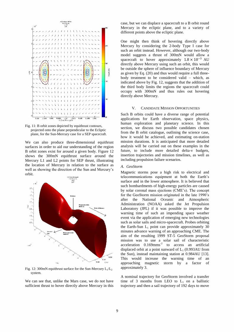
Fig. 11: B orbit zones depicted by equithrust contours,
projected onto the plane perpendicular to the Ecliptic
plane, for the Sun-Mercury case for a SEP spacecraft.
We can also produce three-dimensional equithrust
surfaces in order to aid our understanding of the region
B orbit zones exist for around a given body. Figure 12
shows the 300mN equithrust surface around the
Mercury L1 and L2 points for SEP thrust, illustrating
the location of Mercury in relation to the surface as
well as showing the direction of the Sun and Mercury’s
orbit.
Fig. 12: 300mN equithrust surface for the Sun-Mercury L1/L2
system.
We can see that, unlike the Mars case, we do not have
sufficient thrust to hover directly above Mercury in this
case, but we can displace a spacecraft to a B orbit round
Mercury in the ecliptic plane, and to a variety of
different points above the ecliptic plane.
One might then think of hovering directly above
Mercury by considering the 2-body Type I case for
such an orbit instead. However, although our two-body
model suggests a thrust of 300mN would allow a
spacecraft to hover approximately 1.8 × 10⁻³ AU
directly above Mercury using such an orbit, this would
be outside the sphere of influence boundary of Mercury
as given by Eq. (20) and thus would require a full three-
body treatment to be considered valid – which, as
indicated above by Fig. 12, suggests that the addition of
the third body limits the regions the spacecraft could
occupy with 300mN and thus rules out hovering
directly above Mercury.
V. CANDIDATE MISSION OPPORTUNITIES
Such B orbits could have a diverse range of potential
applications for Earth observation, space physics,
human exploration and planetary science. In this
section, we discuss two possible candidates chosen
from the B orbit catalogue, outlining the science case,
how it would be achieved, and estimating on-station
mission durations. It is anticipated that more detailed
analysis will be carried out on these examples in the
future, to include more detailed delta-v budgets,
insertion trajectories and mission timelines, as well as
including propulsion failure scenarios.
A. GeoStorm
Magnetic storms pose a high risk to electrical and
telecommunications equipment at both the Earth’s
surface and in the lower atmosphere. It is believed that
such bombardments of high-energy particles are caused
by solar coronal mass ejections (CME’s). The concept
for the GeoStorm mission originated in the late 1990’s
after the National Oceanic and Atmospheric
Administration (NOAA) asked the Jet Propulsion
Laboratory (JPL) if it was possible to improve the
warning time of such an impending space weather
event via the application of emerging new technologies
such as solar sails and micro-spacecraft. Probes orbiting
the Earth-Sun L1 point can provide approximately 30
minutes advance warning of an approaching CME. The
aim of the resulting 1999 ST-5 GeoStorm proposal
mission was to use a solar sail of characteristic
acceleration 0.169mms-2
to access an artificial
displaced orbit at a point sunward of L1 (0.993AU from
the Sun), instead maintaining station at 0.984AU [13].
This would increase the warning time of an
approaching magnetic storm by a factor of
approximately 3.
A nominal trajectory for GeoStorm involved a transfer
time of 3 months from LEO to L1 on a ballistic
trajectory and then a sail trajectory of 192 days to move
10
from L1 to sub-L1 [14]. The ST-5 design was not
chosen by NASA for flight demonstration; however, it
did highlight the performance potential. Further work
by JPL [13] involved an improved solar sail design that
would allow a craft of mass approximately 95kg and
characteristic acceleration 0.438mms-2
, to maintain
station at 0.974AU, increasing the warning time yet
further (by another factor of 2 compared to the 1999
mission proposal).
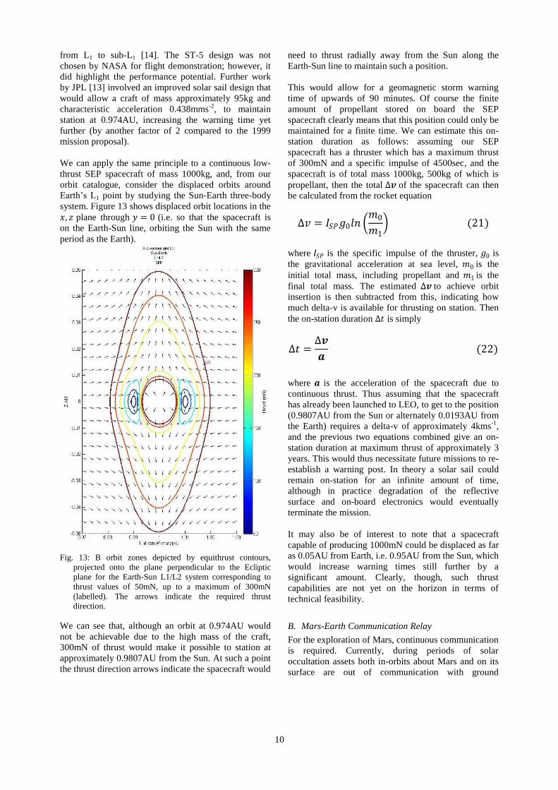
We can apply the same principle to a continuous low-
thrust SEP spacecraft of mass 1000kg, and, from our
orbit catalogue, consider the displaced orbits around
Earth’s L1 point by studying the Sun-Earth three-body
system. Figure 13 shows displaced orbit locations in the
𝑥, 𝑧 plane through 𝑦 = 0 (i.e. so that the spacecraft is
on the Earth-Sun line, orbiting the Sun with the same
period as the Earth).
Fig. 13: B orbit zones depicted by equithrust contours,
projected onto the plane perpendicular to the Ecliptic
plane for the Earth-Sun L1/L2 system corresponding to
thrust values of 50mN, up to a maximum of 300mN
(labelled). The arrows indicate the required thrust
direction.
We can see that, although an orbit at 0.974AU would
not be achievable due to the high mass of the craft,
300mN of thrust would make it possible to station at
approximately 0.9807AU from the Sun. At such a point
the thrust direction arrows indicate the spacecraft would
need to thrust radially away from the Sun along the
Earth-Sun line to maintain such a position.
This would allow for a geomagnetic storm warning
time of upwards of 90 minutes. Of course the finite
amount of propellant stored on board the SEP
spacecraft clearly means that this position could only be
maintained for a finite time. We can estimate this on-
station duration as follows: assuming our SEP
spacecraft has a thruster which has a maximum thrust
of 300mN and a specific impulse of 4500sec, and the
spacecraft is of total mass 1000kg, 500kg of which is
propellant, then the total Δ𝒗 of the spacecraft can then
be calculated from the rocket equation
∆𝑣 = 𝐼𝑆𝑃𝑔0𝑙𝑛 𝑚0
𝑚1 (21)
where 𝐼𝑆𝑃 is the specific impulse of the thruster, 𝑔0 is
the gravitational acceleration at sea level, 𝑚0 is the
initial total mass, including propellant and 𝑚1 is the
final total mass. The estimated Δ𝒗 to achieve orbit
insertion is then subtracted from this, indicating how
much delta-v is available for thrusting on station. Then
the on-station duration Δ𝑡 is simply
Δ𝑡 =Δ𝒗
𝒂 (22)
where 𝒂 is the acceleration of the spacecraft due to
continuous thrust. Thus assuming that the spacecraft
has already been launched to LEO, to get to the position
(0.9807AU from the Sun or alternately 0.0193AU from
the Earth) requires a delta-v of approximately 4kms-1
,
and the previous two equations combined give an on-
station duration at maximum thrust of approximately 3
years. This would thus necessitate future missions to re-
establish a warning post. In theory a solar sail could
remain on-station for an infinite amount of time,
although in practice degradation of the reflective
surface and on-board electronics would eventually
terminate the mission.
It may also be of interest to note that a spacecraft
capable of producing 1000mN could be displaced as far
as 0.05AU from Earth, i.e. 0.95AU from the Sun, which
would increase warning times still further by a
significant amount. Clearly, though, such thrust
capabilities are not yet on the horizon in terms of
technical feasibility.
B. Mars-Earth Communication Relay
For the exploration of Mars, continuous communication
is required. Currently, during periods of solar
occultation assets both in-orbits about Mars and on its
surface are out of communication with ground

11
controllers. While such a scenario is acceptable for
robotic assets it is not for human exploration, and as
such a communication relay is required to ensure
continuous communication between Earth and Mars. It
is noted that any spacecraft within the Ecliptic plane (or
even which passes through the Ecliptic plane) shall
experience periods of solar occultation of Earth, as
such, we must consider non-Keplerian orbits outwith
the Ecliptic plane.
Figure 14 illustrates the architecture options of a Mars-
Earth communication relay, assuming a four-degree
field-of-view exclusion zone about the Sun as viewed
from Earth.
1 au 1.52 au
4˚ 2.6˚
Sun – MarsL1 / L2 HoverSun – Earth
L1 / L2 Hover
Solar Hover
Occulted Region
Ecliptic Plane
Fig. 14: Mars – Earth communication relay architecture
options out of the Ecliptic plane (not to scale).
Note that although points above the Ecliptic plane are
illustrated the architecture is symmetrical about the
Ecliptic plane. For design optimisation of the
communication system, a spacecraft in proximity of
Mars is preferred as the long slant range back to Earth
can be compensated for through the use of a large Earth
based antenna. From Figure 14, note further that hover
points above L2 are slightly further from the Ecliptic
plane, and thus it will require a slight amount of extra
thrust to maintain these points.
The Sun – Mars stations can be determined to be
located approximately 0.176AU out of the Ecliptic
plane (as stated above, assuming a 4-degree field-of-
view exclusion from Earth), while the Sun – Earth
stations can be determined to be located approximately
0.116AU outwith the Ecliptic plane (if the equivalent
spacecraft-Mars-Sun angle is taken to be 2.64°). As
discussed in the previous section, the much shallower
gravitational potential well at Mars significantly
increases the distance from the planet that a spacecraft
can hover at in comparison to Earth.
It is therefore of great interest to note that the value of
0.176AU for a Mars station is just within the range
achievable by a continuous low-thrust spacecraft of
300mN, as illustrated in Figure 15, making a Mars
hover a particularly strong candidate for further study.
(Note that Figure 15 is essentially just the same as
Figure 7, but with additional intermediate contours.)
Fig. 15: B orbit zones depicted by equithrust contours
projected onto the plane perpendicular to the Ecliptic
place for the Mars-Sun three-body system, for SEP of
thrust values of up to 300mN with contours each
representing 10mN.
An interesting extension to this concept is to consider
spacecraft in displaced orbits either leading or trailing
the orbit of Mars, i.e. in the Ecliptic plane. Considering
the symmetry of Figure 14, the 4-degree field-of-view
exclusion defines a conic region around the Sun where
Mars is hidden from the Earth. If we consider this conic
region end-on from behind Mars, as shown in Figure
16, we can consider that, as well as achieving
continuous communications by displacing a spacecraft
directly above Mars, one could also displace a
spacecraft onto the circular (when projected in two
dimensions) region around Mars defined by the field-
of-view exclusion, so that one spacecraft was trailing
and the other leading the orbit of Mars.
0.176au
Occulted Region
B orbit spacecraft trailing Mars
B orbit spacecraft leading Mars
0.176 au
B orbit spacecraft hovering directly above Mars
Plane of Mars orbit
Fig. 16: End-on view of the Mars – Earth communication
relay architecture options, looking into the Ecliptic plane.

12
Naturally, as they track Mars they too will enter the
blackout region: as depicted in Figure 16, the leading
spacecraft will move beyond the edge of the blackout
region as the trailing spacecraft moves into this region.
However, the separation of the two spacecraft means
that only one will ever be in this region at any given
time, and, hence, provided the spacecraft are displaced
far enough above the plane of the orbit of Mars to
maintain a line-of-sight between themselves, as
illustrated in Figure 16, then continual communications
can still be achieved by relaying the signal from the
occulted spacecraft to the one outside the occulted
region and then on to Earth.
There are other advantages to considering this dual
spacecraft option over the case of a single spacecraft
hover. Firstly, hovering directly above Mars limits
communications to just the polar regions. If the
spacecraft are trailing/leading the orbit then
communication with the equatorial regions is enabled.
A second advantage can be shown by considering the
thrust contours in the plane illustrated by Figure 16, i.e.
the y-z plane, as shown in Figure 17.
Fig. 17: An end-on view of B orbit zones depicted by
equithrust contours of up to 300mN about Mars, looking
into the Ecliptic plane. The black circle represents the
extent of the occulted region.
As can be seen it is easier to displace the spacecraft
orbit from Mars in this plane than out of it and so a
spacecraft can occupy a B orbit region on the surface
defined by the field-of-view exclusion for less thrust if
it trails or leads Mars rather than hovering directly
above. So, practically, it may be more feasible to
maintain the communications relay using two
spacecraft with lower thrust than a single spacecraft
which needs higher thrust.
Technically the circular orbit of Mars and the spacecraft
means that the arc drawn out as they pass through the
occulted region is not confined to a single slice in the y-
z plane, but as the arc length is relatively small
compared to the diameter of the orbit it is reasonable to
approximate the arc to a straight line (and thus the
spherical surface, defined by the arc, to a Cartesian
plane) to illustrate the point. A more detailed analysis
of the contours would require projecting contours onto
this spherical surface.
Further, one could potentially induce a non-Keplerian
orbit to displace the spacecraft in either (leading or
trailing) orbit closer to or further from the Earth (see
Figure 18).
1 au 1.52 au
4˚
Occulted Region
Occulted Region
4˚
Orbit Trajectory
0.176 auDisplaced
Displaced B orbit spacecraft trailing Mars A orbit
Displaced
Earth
Fig. 18: Mars – Earth communication relay architecture
options in the Ecliptic plane (not to scale).
We can see that a maximum thrust of 300mN allows a
spacecraft to be displaced up to a maximum of
approximately 0.06AU closer to (or further from) the
Earth, as shown in both Figures 15 and 19, and still
maintain an orbit with the same orbital velocity as that
of Mars, allowing it to track the planet at a constant
distance.
Fig. 19: B orbit zones depicted by equithrust contours,
projected onto the plane parallel to the Ecliptic plane for
the Mars-Sun three-body system in the Ecliptic plane, for
SEP of thrust values of up to 300mN.
13
This displacement is of course dependent on the plane
of the orbit, so displacing higher above Mars makes it
harder to displace closer to Earth. Such a position will
be considered in a detailed mission study because there
is clearly some trade-off to be made between
communicating with a specific region on the surface,
maintaining an optimal line-of-sight between the two
spacecraft, minimising the signal travel time between
the spacecraft and the Earth and doing all this for the
minimum amount of thrust. As an example, consider
the case where, rather than having both spacecraft
above the plane of the orbit Mars one is instead below
this plane, as in Figure 20:
Occulted Region
B orbit spacecraft trailing Mars
B orbit spacecraft leading Mars
0.176 au
Plane of Mars orbit
Fig. 20: End-on view of an alternative Mars – Earth
communication relay architecture option, looking into the
Ecliptic plane.
This configuration would require two spacecraft with
the same thrust as the configuration in Figure 16, but
with the added advantage of covering most of both
hemispheres of Mars, unlike the configuration in Figure
16. Given the distance between the spacecraft, the arc
of the orbit should be sufficient to maintain the line-of-
sight (i.e. one will not be occulted by Mars with respect
to the other) - but if not one could of course displace
them far enough from the planet in the plane of the
orbit of Mars (i.e. towards/away from Earth, as depicted
in Figure 18) to ensure that the line-of-sight is restored,
although this would require more thrust as we would be
displacing away from Mars in two planes, not just one.
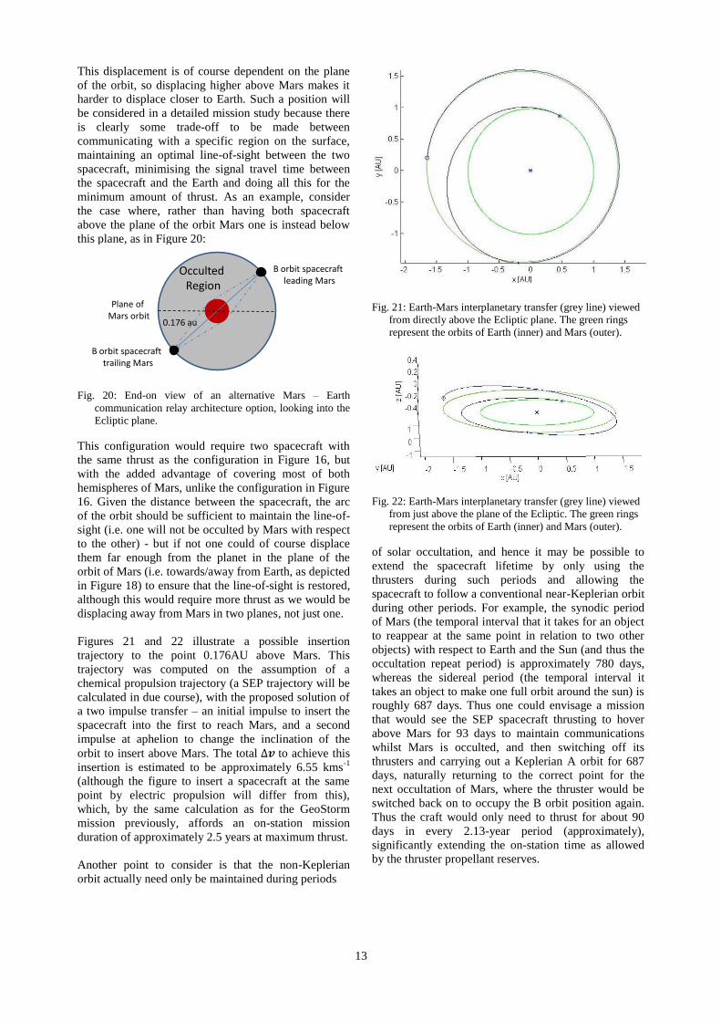
Figures 21 and 22 illustrate a possible insertion
trajectory to the point 0.176AU above Mars. This
trajectory was computed on the assumption of a
chemical propulsion trajectory (a SEP trajectory will be
calculated in due course), with the proposed solution of
a two impulse transfer – an initial impulse to insert the
spacecraft into the first to reach Mars, and a second
impulse at aphelion to change the inclination of the
orbit to insert above Mars. The total Δ𝒗 to achieve this
insertion is estimated to be approximately 6.55 kms-1
(although the figure to insert a spacecraft at the same
point by electric propulsion will differ from this),
which, by the same calculation as for the GeoStorm
mission previously, affords an on-station mission
duration of approximately 2.5 years at maximum thrust.
Another point to consider is that the non-Keplerian
orbit actually need only be maintained during periods
Fig. 21: Earth-Mars interplanetary transfer (grey line) viewed
from directly above the Ecliptic plane. The green rings
represent the orbits of Earth (inner) and Mars (outer).
Fig. 22: Earth-Mars interplanetary transfer (grey line) viewed
from just above the plane of the Ecliptic. The green rings
represent the orbits of Earth (inner) and Mars (outer).
of solar occultation, and hence it may be possible to
extend the spacecraft lifetime by only using the
thrusters during such periods and allowing the
spacecraft to follow a conventional near-Keplerian orbit
during other periods. For example, the synodic period
of Mars (the temporal interval that it takes for an object
to reappear at the same point in relation to two other
objects) with respect to Earth and the Sun (and thus the
occultation repeat period) is approximately 780 days,
whereas the sidereal period (the temporal interval it
takes an object to make one full orbit around the sun) is
roughly 687 days. Thus one could envisage a mission
that would see the SEP spacecraft thrusting to hover
above Mars for 93 days to maintain communications
whilst Mars is occulted, and then switching off its
thrusters and carrying out a Keplerian A orbit for 687
days, naturally returning to the correct point for the
next occultation of Mars, where the thruster would be
switched back on to occupy the B orbit position again.
Thus the craft would only need to thrust for about 90
days in every 2.13-year period (approximately),
significantly extending the on-station time as allowed
by the thruster propellant reserves.

14
Of course the alignment of the planets as shown in
Figure 14 is of course not the complete picture, as the
inclination of the orbit of Mars has to be taken into
account as well. Thus a detailed study is required in
order to determine exactly where Mars would be in
relation to the Ecliptic plane at each occultation:
sometimes Mars may be higher or lower in relation to
the Earth-Sun line, meaning that the distance the
spacecraft would need to hover at above Mars in order
to maintain the communications relay would change,
and thus the amount of thrust required would also
change accordingly. It is also intended that a detailed
propulsion failure scenario study be carried out on this
mission, which will suggest optimal strategies for
recovering a stable orbit in the event of a malfunction.
It may also be possible to use Earth’s L3 point for a
similar purpose. However, it is estimated that 300mN
would only allow the spacecraft to hover a maximum of
approximately 0.05AU above the L3 point (as shown in
Figure 23) compared with the 0.14AU required in order
to achieve continuous communications (again assuming
a four-degree Solar field-of-view exclusion from
Earth).
Fig. 23: B orbit zones depicted by equithrust contours around
the Earth L3 point projected onto the plane parallel to the
Ecliptic plane, for SEP of thrust values of up to 300mN.
The arrows represent the direction of thrust required.
Additionally, it is worth considering the size of
antennae needed for communication between the
spacecraft, the surface of Earth, and the surface of
Mars. Displacing a spacecraft above Earth’s L3 point
would require one large antenna in order to transmit
signals across the sizeable distance of 2AU between the
Earth and the L3 hover point and Mars, as well a
medium-sized antenna for transmission across the
lesser but still significant 0.52AU between the L3 point
and Mars. The advantage of hovering close to Mars is
that whilst one large antenna is still required for
communicating between the spacecraft and Earth,
2.52AU away, the second antenna only has to transmit
signals across the much shorter distance between the
spacecraft and the Martian surface approximately
0.176AU away, or the other (leading or trailing)
spacecraft approximately 0.352AU away and thus need
not be as large.
In theory, yet another possible way of achieving the
same objective would be to consider a Solar hover, i.e.
the two-body Sun-centred displaced B orbit directly
above the Sun in the plane out of the Ecliptic. As
Figure 24 shows, a spacecraft with 300mN of thrust
could hover approximately 4.5AU directly above the
Sun. In real terms though the distance and extreme
difficulty of inserting a spacecraft into such an orbit in
the first place would make this impractical for such a
purpose – however, it demonstrates the potential that
such orbits have.
Fig. 24: Equithrust contours depicting the displaced Type I B
orbit regions about the Sun. The innermost contour
represents a thrust of 300mN (labelled). The dashed lines
represent contours of constant orbital period.

15
VI. SUMMARY
A catalogue of displaced non-Keplerian B orbits for
celestial bodies in the Solar system has been
systematically created. B orbits could have a diverse
range of applications for space physics, exploration and
planetary science and thus such a catalogue is important
in quickly and efficiently determining which
opportunities are enabled by specific spacecraft
parameters, such as mass and maximum thrust. B orbits
are considered both for the two-body case, where three
unique types of orbit exist, parameterised by the orbit
period, and for the three-body case, where the orbit
period of the spacecraft is fixed to that of the planet it is
in the vicinity of. Both solar electric and solar sail
propulsion systems are considered, although in the
latter case only about the Sun in the two-body case or
about a body orbiting the Sun in the three-body case.
The SEP case considers either current or near-term
technology, such as the QinetiQ T6 thruster. Some
example figures are provided and two potential
candidate missions utilising B orbits from the catalogue
are discussed at length.
Of course, it is important to note that although we
consider equithrust surfaces, no propulsion system
actually delivers an equal thrust throughout the lifetime
of the spacecraft, due to either depletion of reaction-
mass or, in the case of solar sailing, the degradation of
the optical surface [15]. As such, the propulsion system
must be throttled to adjust for either the increasing (for
depletion of reaction-mass) or decreasing (for
degradation of the optical surface) acceleration vector
magnitude.
ACKNOWLEDGEMENTS
This work was funded primarily by ESA Contract
Number 22349/09/F/MOS; Study on Gravity Gradient
Compensation Using Low Thrust High Isp Motors and
by European Research Council Advanced Investigator
Grant VISIONSPACE 227571 for C. McInnes.
REFERENCES
[1] H.M. Dusek, “Optimal station keeping at collinear points”, Progress in Astronautics and Aeronautics, 17, 37-44, 1966.
[2] C.R. McInnes, A.J.C. McDonald, J.F.L Simmons, E.W. MacDonald, “Solar sail parking in restricted three-body systems”, Journal of Guidance, Dynamics and Control, Vol 17, No. 2, pp 399-406, 1994
[3] R.L. Forward, “Statite: a spacecraft that does not orbit”, Journal of Spacecraft and Rockets, Vol. 28, No. 5, pp. 606-611, 1991
[4] C.R. McInnes, Solar Sailing: Technology, Dynamics, and Mission Applications, Praxis Publishing, Chichester, 1999, ISBN 1-85233-102-X.
[5] S. Baig, C. R. McInnes, “Artificial three-body equilibria for hybrid low-thrust propulsion”, Journal of Guidance, Control and Dynamics, Vol. 31, No. 6, November-December 2008.
[6] T.R. Spilker, “Saturn ring observer”, Acta Astronautica, Vol. 52, p259-265, 2003
[7] C.R. McInnes, “Dynamics, stability and control of displaced non-Keplerian orbits”, Journal of Guidance, Control, and Dynamics, Vol. 21, No. 5, September-October 1998
[8] J. Simo, C.R. McInnes, “Displaced periodic orbits with low-thrust propulsion in the Earth-Moon System”, AAS 09-153, 19
th AAS/AIAA Space
Flight Mechanics Meeting, Savannah, Georgia, February, 2009.
[9] M. Macdonald, G.W. Hughes, C.R. McInnes, A. Lyngvi, P. Falkner, A. Atzei, “GeoSail: an elegant solar sail demonstration mission”, Journal of Spacecraft and Rockets, Vol. 44, No. 4, July-August 2007
[10] M. Leipold, W. Seboldt, S. Ligner, E. Borg, A. Herrmann, A. Pabsch, O. Wagner, J. Bruckner, “Mercury Sun-synchronous polar orbiter with a solar sail”, Acta Astronautica, Vol. 39, No. 1-4, pp 143-151, 1996
[11] M. Leipold, E. Borg, S. Ligner, A. Pabsch, R. Sachs, W. Seboldt, “Mercury orbiter with a solar sail spacecraft”, Acta Astronautica, Vol 35, pp635-644, 1995
[12] N. Wallace, “Testing of the Qinetiq T6 thruster in support of the ESA BepiColombo Mercury mission”, Proceedings of the 4
th International
Spacecraft Propulsion Conference (ESA SP-555), Chia Laguna, Cagliari, Italy, 2
nd-9
th June 2004
[13] J.L. West, “The GeoStorm warning mission: enhanced opportunities based on new technology”, 14
th AAS/AIAA Spaceflight Mechanics
Conference, Paper AAS 04-102, Maui, Hawaii, Feb 8
th-12
th 2004
[14] J.L. West, “Solar sail vehicle system design for the GeoStorm warning mission”, Structures, Structural Dynamics and Materials Conference, Atlanta, USA, April 2000
[15] B. Dachwald, M. Macdonald, C.R. McInnes, G. Mengali, A.A. Quarta, “Impact of optical degradation on solar sail mission performance”, Journal of Spacecraft and Rockets, Vol 44., No. 4, pp740-749,2007
Recommended