NON-REDUNDANT APERTURE MASKING
INTERFEROMETRY WITH ADAPTIVE OPTICS:
DEVELOPING HIGHER CONTRAST IMAGING TO
TEST BROWN DWARF AND EXOPLANET
EVOLUTION MODELS
A Dissertation
Presented to the Faculty of the Graduate School
of Cornell University
in Partial Fulfillment of the Requirements for the Degree of
Doctor of Philosophy
by
David Bernat
January 2012

c© 2012 David Bernat
ALL RIGHTS RESERVED
NON-REDUNDANT APERTURE MASKING INTERFEROMETRY WITH
ADAPTIVE OPTICS: DEVELOPING HIGHER CONTRAST IMAGING TO
TEST BROWN DWARF AND EXOPLANET EVOLUTION MODELS
David Bernat, Ph.D.
Cornell University 2012
This dissertation presents my study of Non-Redundant Aperture Masking Interfer-
ometry (or NRM) with Adaptive Optics, a technique for obtaining high-contrast
infrared images at diffraction-limited resolution. I developed numerical, statisti-
cal, and on-telescope techniques for obtaining higher contrast, in order to build an
imaging system capable of resolving massive Jupiter analogs in tight orbits around
nearby stars. I used this technique, combined with Laser Guide Star Adaptive Op-
tics (LGSAO), to survey known brown dwarfs for brown dwarf and planetary com-
panions. The diffraction-limited capabilities of this technique enable the detection
of companions on short period orbits that make Keplerian mass measurement prac-
tical. This, in turn, provides mass and photometric measurements to test brown
dwarf evolution (and atmosphere) models, which require empirical constraints to
answer key questions and will form the basis for models of giant exoplanets for the
next decade.
I present the results of a close companion search around 16 known brown dwarf
candidates (early L dwarfs) using the first application of NRM with LGSAO on
the Palomar 200” Hale Telescope. The use of NRM allowed the detection of com-
panions between 45-360 mas in Ks band, corresponding to projected physical sep-
arations of 0.6-10.0 AU for the targets of the survey. Due to unstable LGSAO
correction, this survey was capable of detecting primary-secondary contrast ratios
down to ∆Ks ∼1.5-2.5 (10:1), an order of magnitude brighter than if the system
performed at specification. I present four candidate brown dwarf companions de-
tected with moderate-to-high confidence (90%-98%), including two with projected
physical separations less than 1.5 AU. A prevalence of brown dwarf binaries, if con-
firmed, may indicate that tight-separation binaries contribute to the total binary
fraction more significantly than currently assumed, and make excellent candidates
for dynamical mass measurement. For this project, I developed several new, ro-
bust tools to reject false positive detections, generate accurate contrast limits, and
analyze NRM data in the low signal-to-noise regime.
In order to increase the sensitivity of NRM, a critical and quantitative study
of quasi-static wavefront errors needs to be undertaken. I investigated the impact
of small-scale wavefront errors (those smaller than a sub-aperture) on NRM using
a technique known as spatial filtering. Here, I explored the effects of spatial fil-
tering through calculation, simulation, and observational tests conducted with an
optimized pinhole and aperture mask in the PHARO instrument at the 200” Hale
Telescope. I find that spatially filtered NRM can increase observation contrasts by
10-25% on current AO systems and by a factor of 2-4 on higher-order AO systems.
More importantly, this reveals that small scale wavefront errors contribute only
modestly to the overall limitations of the NRM technique without very high-order
AO systems, and that future efforts need focus on temporal stability and wavefront
errors on the scale of the sub-aperture. I also develop a formalism for optimizing
NRM observations with these AO systems and dedicated exoplanet imaging instru-
ments, such as Project 1640 and the Gemini Planet Imager. This work provides a
foundation for future NRM exoplanet experiments.
BIOGRAPHICAL SKETCH
David Bernat started along a trajectory towards this point early, but cemented his
direction shortly after watching the Mars Pathfinder and Sojourner rover land on
the surface of Mars on July 4, 1997. Later that fall, he attended the California Insti-
tute of Technology to earn a Physics B.S. while immersed in a spirited and creative
scientific and academic environment. After considering multiple post-graduation
options in science and engineering, but wanting to explore an application of physics
outside the academic environment, he moved to New York City in 2002 to work as a
strategist at Goldman Sachs in the Foreign Exchange, Currency, and Commodities
sector. This opportunity became one of the most striking and stimulating expe-
riences of his life so far. Watching the operation of the global financial machine
from the inside-out during one of the most contentious and complex times during
the aftermath of 9/11 and the run-up to the Iraq War has shaped his view of the
world, civic citizenry, and the growth potential of well-administered organizations.
He worked on projects ranging from price evaluations of derivatives on the Federal
Reserve Interest Rate to projections of risk and loss by corporate and catastrophic
default. In 2004, he left Goldman Sachs to move to Munich, Germany, to provide
technical support at the Max Planck Institute for Physics and the DESY particle
accelerator while applying to graduate schools. The following year, he began his
study at Cornell University. Following his early passion for quantum mechanics
and general relativity, he quickly began researching with Prof. Rachel Bean to
investigate modification to General Relativity that could give rise to the perceived
cosmological acceleration of the Universe observed today. One research paper later,
and upon hearing that space-based spectrographs had just detected the presence
of water gas in the atmosphere of a planet in another solar system, he moved four
floors downward to start his graduate research with Prof. James Lloyd.
iii

As a scientist, David’s primary ambition is to conduct research. Yet he feels
strongly that a key component to being an effective scientist is a desire to com-
municate research and to generate the development of teaching programs and the
scientific community. During his six years at Cornell University, he maintained ac-
tive roles in the Physics Graduate Society, Astronomy Graduate Network, and the
Graduate and Professional Student Assembly. He wrote for the Ask an Astronomer
@ Cornell service, and has written and produced for the Ask an Astronomer Pod-
cast series. For his successful completion of science journalism courses and a pub-
lishing prospectus for a book on exoplanets, David earned a Science Communica-
tion minor at Cornell. David completed this dissertation in September 2011.
iv
To my parents, who put a good head on my shoulders.
To my friends, who helped keep it there.
v
ACKNOWLEDGEMENTS
Like any pursuit into the challenging and unknown, I am thankful for the friends
and colleagues who shared in the venture. This page describes all the people I
have to thank for helping me complete the trip and for adding to the pleasure of
the journey.
Professional Acknowledgements
Many colleagues in the scientific community contributed to various aspects of this
dissertation and helped to make this work larger than the sum of my ideas. For
their scientific advice, I extend my gratitude to the members of my dissertation
committee: James Lloyd, Ira Wasserman, Ivan Bazarov, and Bruce Lewenstein. I
benefited from multiple discussions and pieces of guidance from each one of them,
and in particular James Lloyd, my dissertation advisor, for his supervision and for
demanding the best research from me.
I would like to thank Peter Tuthill, Michael Ireland, and Frantz Martinache,
my collaborators in the small world of NRM, for teaching me the basics in my
fledgeling graduate days and then numerous suggestions and recalibrations of di-
rection throughout this work.
I have enjoyed countless spirited and informative conversations with excellent
scientists at and beyond my university which have been integral to my development
as a scientist. In particular, I would like to point out Jason Wright, who provided
several key elements to my first NRM publication and whose acute understanding
of our field enabled him to point out the constellations among my pinpoints of
ideas. I am especially grateful to Peter Tuthill and Anand Sivaramakrishnan for
providing needed perspective throughout the last two years and for allowing me to
learn countless intangibles from their seemingly unending supply of wisdom.
vi
In addition, I am indebted to the staff at Palomar Observatory, including Jean
Mueller, for her long and dedicated night-time hours and quick operation at the
controls. I am grateful to Jeff Hickey, Rich DeKany, Antonin Bouchez, and the
Palomar AO Team for keeping the control room spirited and developing the excel-
lent instruments which serve as the backbone for this research. And, finally, Laurie
McCall, who confirms that no successful operation runs without steady support
behind the scenes.
I would also like to thank my first graduate advisor, Rachel Bean, for indulging
my eagerness to explore general relativity and for leading me through my first
whirlwind year as a graduate student and my first publication. She showed me
that with patience, genuiousity, and depth of skill, that I can grow in leaps and
bounds; her hands-on-style helped affirm my own teaching and mentorship style
that has rewarded me so today.
UnProfessional Acknowledgements
In both undergraduate and graduate school, I have been fortunate to have been
immersed in an amazing, vibrant scientific and social environment that continually
provided opportunities to befriend wonderful people and scientists. These friends
and colleagues shared in my joys and troubles; provided ballast, beers, and dis-
tractions; and generally made my day to day experiences more joyful. I couldn’t
have done this without you, nor would I have chosen to. You know who you are.
Thank you.
Many thanks to my cohort at Caltech, and I hope we maintain an enduring
enthusiasm for all things science and civic.
In six years at Cornell, I taught ten semesters of students in physics and astron-
omy. My students perpetually reminded me that science will always be a subject
of public curiosity. They gave me a place to direct my creative and productive
vii

energies when those energies could not be productively directed toward research.
(As research – unlike my students – has shown at times to be fitful, cranky, unco-
operative, and rather impartial to my enthusiasms). Without their time to develop
a skill set for teaching and mentoring, graduate school would have been a much
more selfish and isolated endeavor.
I am thankful to Ann Martin, Laura Spitler, and David Kornreich for maintain-
ing the Ask An Astronomer @ Cornell service, which has shown me that some of
the hardest questions of all come from middle school children and retired engineers.
And finally, most importantly, I am thankful to my mom and dad for repeatedly
indulging my wild-eyed naive desire and decision to enter the astronomy profession,
despite the long incongruous hours and too-lengthy stays away from home in their
times of need. Nothing in this work would have been possible without them and
their constant support that reaches far beyond any description on this page.
viii
TABLE OF CONTENTS
Biographical Sketch . . . . . . . . . . . . . . . . . . . . . . . . . . . . . . iiiDedication . . . . . . . . . . . . . . . . . . . . . . . . . . . . . . . . . . . vAcknowledgements . . . . . . . . . . . . . . . . . . . . . . . . . . . . . . viTable of Contents . . . . . . . . . . . . . . . . . . . . . . . . . . . . . . . ixList of Tables . . . . . . . . . . . . . . . . . . . . . . . . . . . . . . . . . xiiList of Figures . . . . . . . . . . . . . . . . . . . . . . . . . . . . . . . . . xiii
1 Perspective 11.1 Directly Imaging Faint Companions to Stars . . . . . . . . . . . . . 11.2 Brown Dwarfs as Massive Exoplanet Analogs . . . . . . . . . . . . . 81.3 The Organization of This Manuscript . . . . . . . . . . . . . . . . . 12
2 Brown Dwarfs 142.1 How does one identify a brown dwarf? . . . . . . . . . . . . . . . . 142.2 The Current State of Brown Dwarf Atmosphere and Evolution Models 162.3 Using Mass Measurements to Test Evolution Models . . . . . . . . 262.4 The Challenge of Resolving Brown Dwarf Binaries . . . . . . . . . . 34
2.4.1 Angular Resolution for Brown Dwarf Dynamical Masses . . 352.4.2 Primary-Secondary Contrasts for Brown Dwarf Companions 362.4.3 Adaptive Optics: Resolution . . . . . . . . . . . . . . . . . . 392.4.4 Adaptive Optics: Contrast . . . . . . . . . . . . . . . . . . . 48
3 Non-Redundant Aperture Masking Interferometry with AdaptiveOptics 553.1 Non-Redundant Aperture Masking Interferometry . . . . . . . . . . 573.2 Observing Binaries with an Aperture Mask . . . . . . . . . . . . . . 70
3.2.1 Closure Phase Signal . . . . . . . . . . . . . . . . . . . . . . 703.2.2 Robust Measurement of Binary Parameters and Confidence
Intervals . . . . . . . . . . . . . . . . . . . . . . . . . . . . . 743.2.3 Calculation of Contrast Limits . . . . . . . . . . . . . . . . . 79
4 A Close Companion Search around L Dwarfs using ApertureMasking Interferometry and Palomar Laser Guide Star AdaptiveOptics1 824.1 Abstract . . . . . . . . . . . . . . . . . . . . . . . . . . . . . . . . . 824.2 Introduction . . . . . . . . . . . . . . . . . . . . . . . . . . . . . . . 834.3 Observations and Data Analysis . . . . . . . . . . . . . . . . . . . . 86
4.3.1 Observations . . . . . . . . . . . . . . . . . . . . . . . . . . 864.3.2 Aperture Masking Analysis and Detection Limits . . . . . . 89
4.4 Sixteen Brown Dwarf Targets - Four Candidate Binaries . . . . . . 1034.5 Discussion: Aperture Masking of Faint Targets . . . . . . . . . . . . 1054.6 Conclusion . . . . . . . . . . . . . . . . . . . . . . . . . . . . . . . . 107
ix
5 The Use of Spatial Filtering with Aperture Masking Interferom-etry and Adaptive Optics1 1125.1 Abstract . . . . . . . . . . . . . . . . . . . . . . . . . . . . . . . . . 1125.2 Introduction . . . . . . . . . . . . . . . . . . . . . . . . . . . . . . . 1135.3 Aperture Masking with Spatial Filtering . . . . . . . . . . . . . . . 116
5.3.1 Aperture Masking: Current Technique . . . . . . . . . . . . 1165.3.2 Aperture Masking: Why Spatial Filter? Calibration Errors. 1175.3.3 Pinhole Filtering . . . . . . . . . . . . . . . . . . . . . . . . 1205.3.4 Post-Processing with a Window Function . . . . . . . . . . . 125
5.4 Simulated Observations . . . . . . . . . . . . . . . . . . . . . . . . . 1265.4.1 Characterization and Simulation of Palomar’s Atmosphere . 1275.4.2 Numerical Simulation . . . . . . . . . . . . . . . . . . . . . . 128
5.5 The Palomar Pinhole Experiment . . . . . . . . . . . . . . . . . . . 1305.5.1 Pinhole Implementation on PHARO . . . . . . . . . . . . . 1305.5.2 Pinhole Size Optimization . . . . . . . . . . . . . . . . . . . 1305.5.3 How Important Is Target Placement? . . . . . . . . . . . . . 1325.5.4 Window Function: Optimal Size and the Palomar 9-Hole Mask133
5.6 Observations . . . . . . . . . . . . . . . . . . . . . . . . . . . . . . . 1355.6.1 Pinhole Stability and Target Alignment . . . . . . . . . . . . 1375.6.2 Calibrators: Pinhole Filtering Produces Lower Closure
Phase Variance and Higher Amplitudes . . . . . . . . . . . . 1385.6.3 Binaries: Lower Closure Phase Variance . . . . . . . . . . . 139
5.7 Summary of Results and Conclusions . . . . . . . . . . . . . . . . . 1485.8 Discussion . . . . . . . . . . . . . . . . . . . . . . . . . . . . . . . . 152
5.8.1 A Strategy for Future Pinhole Observations . . . . . . . . . 1525.8.2 Extreme-AO Aperture Masking Experiments . . . . . . . . . 153
Acknowledgements . . . . . . . . . . . . . . . . . . . . . . . . . . . . . . 1545.9 Pinhole Filtering: Inteferometry . . . . . . . . . . . . . . . . . . . . 1605.10 Spatial Structure of Closure Phase Redundancy Noise . . . . . . . . 162
5.10.1 Baseline Visibility Measurement . . . . . . . . . . . . . . . . 1645.10.2 Instantaneous Closure Phase . . . . . . . . . . . . . . . . . . 166
6 Synthesis and Conclusions 1706.1 Refinement of the NRM with AO Technique: Results . . . . . . . . 1716.2 Refinement of the NRM with AO Technique: Future Work . . . . . 1726.3 Study of Brown Dwarf Binaries using LGSAO: Results . . . . . . . 1756.4 Study of Brown Dwarf Binaries using LGSAO: Future Work . . . . 1776.5 Future Explorations: Probing Evolution and Formation of Brown
Dwarfs and Massive Jupiter Exoplanets . . . . . . . . . . . . . . . . 1796.5.1 New Paradigms of Planet Formation Driven by Direct Imaging1796.5.2 A Growing Population of Nearby, Young Stars . . . . . . . . 1806.5.3 Feasibility of the Survey with Exoplanet Instruments and
NRM . . . . . . . . . . . . . . . . . . . . . . . . . . . . . . . 1816.6 Conclusions . . . . . . . . . . . . . . . . . . . . . . . . . . . . . . . 182
x

A Primer: Imaging Through a Turbulent Atmosphere with AdaptiveOptics 186A.1 The Point Spread Function . . . . . . . . . . . . . . . . . . . . . . . 186A.2 Atmospheric Turbulence and Adaptive Optics . . . . . . . . . . . . 189
A.2.1 Kolmogorov Turbulence . . . . . . . . . . . . . . . . . . . . 189A.3 Adaptive Optics . . . . . . . . . . . . . . . . . . . . . . . . . . . . . 195
xi
LIST OF TABLES
2.1 Techniques For Resolving Closely Separated Brown Dwarf Com-panions . . . . . . . . . . . . . . . . . . . . . . . . . . . . . . . . . 41
2.2 Pros and Cons of Primary Type . . . . . . . . . . . . . . . . . . . 412.3 Survey Types For Brown Dwarf Companion Searches . . . . . . . . 41
4.1 The Sixteen Very Low Mass Survey Targets . . . . . . . . . . . . . 1004.2 Coordinates and characteristics of the sixteen very low mass tar-
gets observed in this sample. Photometry is taken from the 2MASScatalog. Spectral types (spectroscopic) and distances are takenfrom DwarfArchives.org, unless otherwise noted. aDistance mea-surements derived from J-band photometry and MJ/SpT calibra-tion data of Cruz et al. (2003) assuming a spectral type uncertaintyof ±1 subclass. bSurvey detection limits of Table 4.3 given in termsof secondary-primary mass ratio, assuming a co-eval system (sameage and metalicity). Masses ratios are derived from the 5-Gyr (firstrow) and 1-Gyr (second row), solar-metalicity substellar DUSTYmodels of Chabrier et al. (2000), using J and K band photome-try. s1Target previously observed by Reid et al. (2006). s2Targetpreviously observed by Bouy et al. (2003) . . . . . . . . . . . . . . 100
4.3 Survey Contrast Limits (∆K) at 99.5% Confidence . . . . . . . . . 1014.4 Detection contrast limits around primaries: aPrimary-Secondary
separations are given in units of mas, and the corresponding detec-tion limits are in ∆K magnitudes. . . . . . . . . . . . . . . . . . . 101
4.5 Model Fits to Candidate Binaries . . . . . . . . . . . . . . . . . . . 102
5.1 Observation of Known Binaries With and Without Spatial Filter . 1425.2 Astrometry and Alignment of Targets within Pinhole . . . . . . . . 1435.3 Alignment of Targets Within Pinhole and Estimated Closure Phase
Misalignment Error. Position determined by center of interfero-grams, errors estimated from spread over twenty images. Valuesin parentheses include 40 mas uncertainty of the absolute pinholeposition. Misalignment errors are calculated using the simulationof Section 5.5.3, assuming a Strehl of 15% in H and CH4s, 45% inKs and Brγ, and 10% in J band. . . . . . . . . . . . . . . . . . . . 143
xii

LIST OF FIGURES
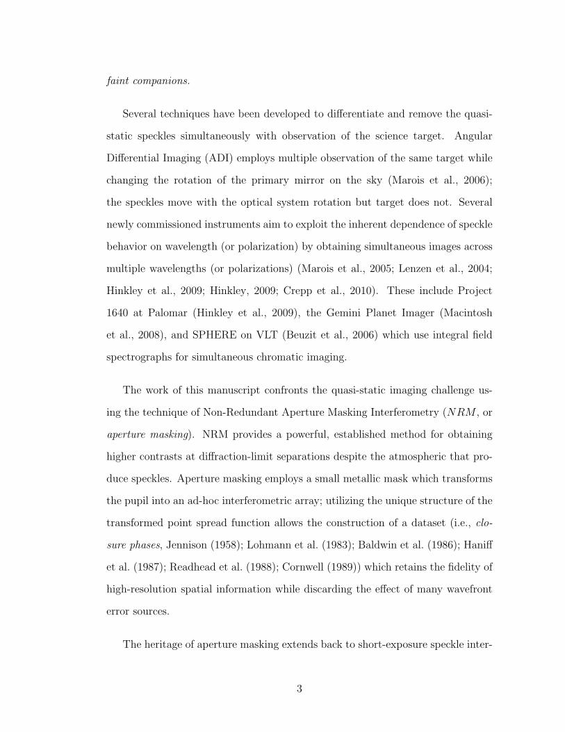
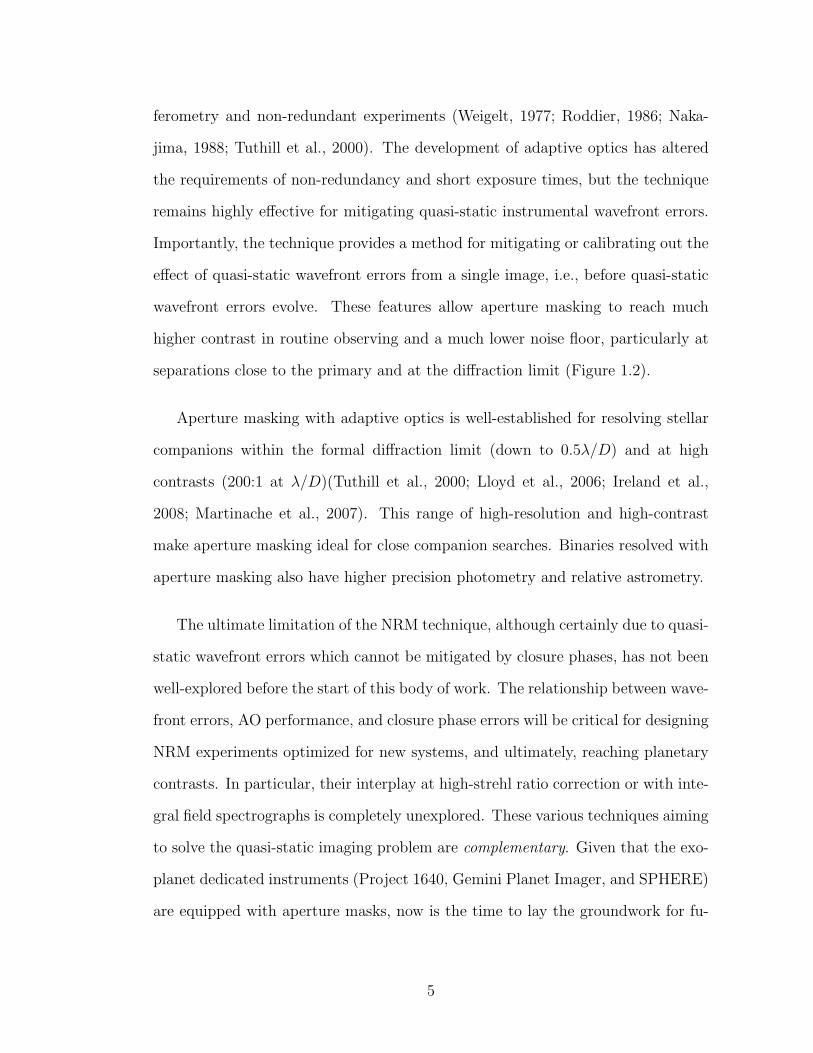
1.1 Close-up of the diffraction core and first and second Airy rings of 6second exposures of HIP 52942, taken with the Palomar AO systemand PHARO instrument. The field of view is 600 mas. Contoursare peak intensity divided by 1.05, 1.18, 1.33, 2., 2.5, 3.33, 5., 10.,20., and 50. Each row contains three images taken roughly ten sec-onds apart. The middle and bottom rows have sets of images taken1 and 10 minutes after the first row, respectively. The tendency ofspeckles to ’pin’ to the Airy rings is readily apparent, as well as athree-fold and four-fold symmetry of the speckle locations on thefirst Airy ring which evolves on minute timescales. (For instance,between the first and second image of the first row.) These pro-duce flux variations as much as 10% of the peak (seventh contour).Variations on the second Airy ring of as much as 2-5% are alsoobserved. These quasi-static speckles limit the image contrast. . . 4
1.2 Comparison of imaging techniques in infrared H Band (Strehl ∼20%) at Palomar Hale 200” Telescope. Aperture Masking (red)routinely achieves ∆H∼5.5 magnitudes (150:1) at the diffractionlimit, much better than direct imaging alone (black). Coronagra-phy (blue), although capable of providing very high contrast is ob-scured at close separations by its Lyot stop. High contrast at closeseparations is crucial for the detection of brown dwarfs for dynam-ical mass measurements. An M-Brown dwarf binary (Contrast ∼4.0-5.0 magnitudes, 80-100:1) cannot be detected by direct imagingat a separation closer than about 3 λ/D; the system would have aperiod of at least 9 years. Aperture Masking can detect these bina-ries over a more expansive range, and with much shorter periods.Companions detected by coronagraphy are rarely able to providedynamical masses. . . . . . . . . . . . . . . . . . . . . . . . . . . . 6
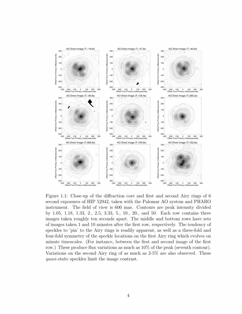
1.3 Comparison of a resolved binary with direct imaging (left) and aper-ture masking (right). Good wavefront correction by the adaptiveoptics system reveals a sharp, Airy function point spread function,though the first Airy ring partially obscures the presence of a 6:1companion (at an angle of 25 degrees counterclockwise of horizon-tal). Even with good correction, speckles are visible, including onepinned to the Airy ring at due south. The large aperture maskingpoint spread function contains many features; these are not speck-les, but rather well-defined structure which allows for the calibratedremoval of wavefront noise. Although no companion is identifiableby eye, processing of the aperture masking image clearly revealsthe presence of the companion, with much higher precision. . . . . 7
xiii
2.1 Color-magnitude diagrams of substellar objects plotted againstmodeled atmospheres and blackbody curves. (Left) Absolute Jv. J-K color magnitude diagram. Curves indicate theoreticalisochrones for substellar objects at ages of 0.5, 1.0, and 5.0 Gyrthrough a range of masses using the brown dwarf models of Bur-rows et al. (1997) and their blackbody counterpart. The differencebetween blackbody colors and model colors is immediately appar-ent. The prototype T dwarf, Gl 229B, and prototype L dwarf, GD165B, are plotted for comparison. Notice that the L dwarf doesnot show an indication of particularly bluer-than-blackbody colors.(Right) Absolute J v. J-H color magnitude diagram. Figure fromBurrows et al. (1997) . . . . . . . . . . . . . . . . . . . . . . . . . . 17
2.2 Bolometric correction for K band photometry and Effective tem-perature as functions of spectral type from Golimowski et al. (2004)(Top) Bolometric corrections can be used to obtain total luminos-ity, Lbol, from K band photometry. (Bottom) By making certainassumptions about the brown dwarf radius, effective temperaturecan be estimated from total luminosity. (See text.) Notice theplateau of temperature marking the transition from L and T dwarfclasses . . . . . . . . . . . . . . . . . . . . . . . . . . . . . . . . . . 21
2.3 Infrared photometry of low mass stars as a function of effectivetemperature. Photometric colors are primarily a function of ef-fective temperature and predominantly dependent on the physicalchemistry of the brown dwarf atmospheres. In the absence of spec-tra, broadband photometric colors are a proxy for spectral typeand temperature. Low mass curves (M0 and later) use photom-etry of Baraffe et al. (2003) and the spectral type-MJ relation ofCruz et al. (2003). High mass curves use the mass-luminosity re-lations of Henry & McCarthy (1993). The infrared photometry ofa blackbody is drawn for comparison; the infrared flux brighteningof dusty stars (M6 and later) and brown dwarfs is readily apparent. 23
2.4 Evolution of luminosity tracks for low mass stars (blue), browndwarfs (green), and planets (red) from Burrows et al. (1997). Ob-ject masses (in Msun) are marked at the right-side end of the tracks.The top set of lines (0.08-0.20 Msun) trace out the evolution of lowmass stars; note the onset of fusion at 0.5-1.0 Gyr and further sta-bilization of luminosity, while brown dwarfs continue to dim. Theshoulder of brief, but constant luminosity early in the evolution ofstars and brown dwarfs signals the brief fusion of primordial deu-terium. . . . . . . . . . . . . . . . . . . . . . . . . . . . . . . . . . 27
xiv
2.5 Evolution of effective temperature for low mass stars (blue), browndwarfs (green), and planets (red) from Burrows et al. (2001). Thesesets of lines are the same as in Figure 2.4. Horizontal lines markthe evolution from spectra classes M to L and L to T. Note that thelowest mass hydrogen burning stars evolve into L dwarfs, and thatall brown dwarfs start as M dwarfs. Because brown dwarfs evolvethrough to later spectral types for the entirety of their lifetime,unlike stars which stabilize after ∼ 1 Gyr, spectral type without ageis a poor indicator of brown dwarf mass. The orange filled circlesmark the 50% depletion of deuterium; the magenta circles mark the50% depletion of lithium. Since brown dwarfs less massive than ∼0.060 Msun never deplete their primordial lithium, the presence oflithium in L dwarf spectra is an indicator that the object is a browndwarf. . . . . . . . . . . . . . . . . . . . . . . . . . . . . . . . . . . 28
2.6 Effective Temperature as a function of mass for low mass starsand brown dwarfs using the evolutionary models of Baraffe et al.(2003). Unlike stellar objects, the temperatures of brown dwarfscool significantly with age; for any temperature derived from pho-tometry, nearly every brown dwarf mass may be passible if age isnot constrained. Conversely, while temperature changes rapidlyearly, brown dwarfs cool more slowly after several billion years,and precisely measured masses (∼10%) give little constraint to age.Low mass curves (M0 and later) use photometry of Baraffe et al.(2003) and the spectral type-MJ relation of Cruz et al. (2003).High mass curves use the mass-luminosity relations of Henry &McCarthy (1993). . . . . . . . . . . . . . . . . . . . . . . . . . . . 29
2.7 Infrared photometry of low mass stars and brown dwarfs (J band,blue; K band, red) using the models of Baraffe et al. (2003). Eightmagnitudes (1500:1 Flux Ratio) separate solar mass stars and themost massive brown dwarfs at an age of 1 Gyr. Brown dwarfs dimwith age, spanning roughly eight magnitudes between 100 Myr and5 Gyr. Low mass stars and L dwarfs are red in infrared color, thischanges rapidly at the onset of the T dwarf spectral class. . . . . . 30
2.8 Orbital period for a 0.070 M� brown dwarf companion as a functionof semi-major axis and primary spectral type. Wide-separated bi-naries orbit too slowly to track their orbits (and obtain dynamicalmasses) in a practical length of time. In order to obtain the systemmass measurements in less than five years of observing, binarieswith physical separations less than 3 AU need to be targeted. . . . 37
xv

2.9 Primary-Secondary Contrast Ratio of Binary Systems. Clearly,late-type stars offer more favorable contrast ratios than solar typestars. Particularly noteworthy is the rapid drop in brightness (afactor of 100) moving from L0 dwarfs (massive brown dwarfs) toT5 dwarfs (lighter brown dwarfs). Probing the entire mass rangeof brown dwarfs requires very high contrasts in the most favorableof cases. . . . . . . . . . . . . . . . . . . . . . . . . . . . . . . . . . 40
2.10 Contrast and Resolution of Direct AO Imaging is inhibited byspeckle noise, a diffraction effect of wavefront errors, and not pho-ton noise. (Left) Total of 150 one second exposures of HIP 52942in H band on April 12, 2009 (Strehl ∼ 20%). The first and secondAiry ring can be clearly seen, as well as a diffuse halo pepperedwith speckles. A black circle is drawn at 1.22λ/2ra using the AOactuator spacing for ra. This approximates the extent of the halo.(Right) The variance of each pixel is calculated as a function of dis-tance from the primary and averaged azimuthally. The measuredvariance is compared to the calculated photon noise for the pointspread function. As seen, speckle noise is a factor of ∼30x higherthan photon noise. NRM/Aperture masking leads to an increase incontrast precisely because closure phases are able to calibrate outthe effect of these speckle-producing wavefront errors. This figureis an empirical analog to Racine et al. (1999), Fig. 2. . . . . . . . 43
2.11 Absolute visual magnitude as a function of spectral type. Latetype stars and brown dwarfs grow quickly faint in the visible andare too faint to drive adaptive optics systems. For this reason,companion searches which aim image with high angular-resolution(e.g. for dynamical mass measurements) must use primaries earlier(and brighter) than about M3 if natural guide stars are to be used. 47
2.12 Close-up of the diffraction core and first and second Airy rings of 6second exposures of HIP 52942, taken with the Palomar AO systemand PHARO instrument. The field of view is 300 mas in radius,roughly that necessary to resolve binaries with periods short enoughto measure brown dwarf masses. Contours are peak intensity di-vided by 1.05, 1.18, 1.33, 2., 2.5, 3.33, 5., 10., 20., and 50. Eachrow contains three images taken roughly ten seconds apart. Themiddle and bottom rows have sets of images taken 1 and 10 min-utes after the first row, respectively. The tendency of speckles topin to the Airy rings is readily apparent, as well as a three-fold andfour-fold symmetry of the speckle locations on the first Airy ringwhich evolves on minute timescales. (Between, for instance, thefirst and second image of the first row.) These produce flux varia-tions as much as 10% of the peak (seventh contour). Variations onthe second Airy ring of as much as 2-5% are also observed. Thesequasi-static speckles limit the image contrast. . . . . . . . . . . . . 50
xvi
2.13 Primary-Secondary Contrast Ratio Detectable with Direct AOImaging. The fundamental challenge of high contrast direct imag-ing at high angular resolution is to distinguish quasi-static speck-les from true companions. Because quasi-static speckles vary tooslowly to average out, it is their mean brightness that sets thecompanion detection limit. These speckles can be up to 10% peakbrightness at the location of the first Airy ring. Above is the detec-tion contrast limit imposed by quasi-static speckles for 10 minutesof direct imaging of HIP 52942 in H band. NRM achieves highercontrasts not by distinguishing companions from speckles, but bygenerating an observable that is not affected by the wavefront errorswhich produce the speckles (i.e, closure phases) . . . . . . . . . . . 51
2.14 Comparison of imaging techniques in infrared H Band (Strehl ∼20%) at Palomar Hale 200” Telescope. Aperture Masking (red)routinely achieves ∆H∼5.5 magnitudes (150:1) at the diffractionlimit, much better than direct imaging alone (black). Coronagra-phy (blue), although capable of providing very high contrast is ob-scured at close separations by its Lyot stop. High contrast at closeseparations is crucial for the detection of brown dwarfs for dynam-ical mass measurements. An M-Brown dwarf binary (Contrast ∼4.0-5.0 magnitudes, 80-100:1) cannot be detected by direct imagingat a separation closer than about 3 λ/D; the system would have aperiod of at least 9 years. Aperture Masking can detect these bina-ries over a more expansive range, and with much shorter periods.Companions detected by coronagraphy are rarely able to providedynamical masses. . . . . . . . . . . . . . . . . . . . . . . . . . . . 52
3.1 The sparse, non-redundant aperture mask used for observations atthe Hale 200” Telescope at Palomar Observatory. Each pair ofsub-apertures acts as an interferometer of a unique baseline lengthand orientation. Overdrawn is one such baseline. The 9-hole maskproduces thirty-six baselines total; the point spread function of themask is a set of thirty-six overlapping fringes underneath a largeAiry envelope. . . . . . . . . . . . . . . . . . . . . . . . . . . . . . 58
xvii
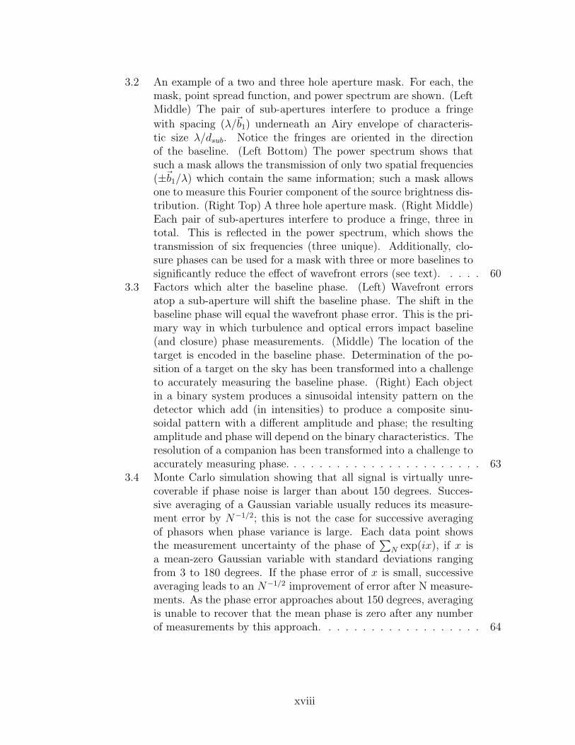
3.2 An example of a two and three hole aperture mask. For each, themask, point spread function, and power spectrum are shown. (LeftMiddle) The pair of sub-apertures interfere to produce a fringe
with spacing (λ/~b1) underneath an Airy envelope of characteris-tic size λ/dsub. Notice the fringes are oriented in the directionof the baseline. (Left Bottom) The power spectrum shows thatsuch a mask allows the transmission of only two spatial frequencies(±~b1/λ) which contain the same information; such a mask allowsone to measure this Fourier component of the source brightness dis-tribution. (Right Top) A three hole aperture mask. (Right Middle)Each pair of sub-apertures interfere to produce a fringe, three intotal. This is reflected in the power spectrum, which shows thetransmission of six frequencies (three unique). Additionally, clo-sure phases can be used for a mask with three or more baselines tosignificantly reduce the effect of wavefront errors (see text). . . . . 60
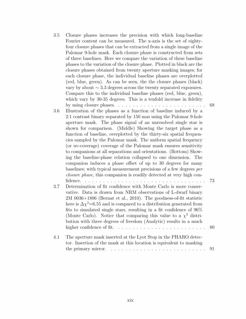
3.3 Factors which alter the baseline phase. (Left) Wavefront errorsatop a sub-aperture will shift the baseline phase. The shift in thebaseline phase will equal the wavefront phase error. This is the pri-mary way in which turbulence and optical errors impact baseline(and closure) phase measurements. (Middle) The location of thetarget is encoded in the baseline phase. Determination of the po-sition of a target on the sky has been transformed into a challengeto accurately measuring the baseline phase. (Right) Each objectin a binary system produces a sinusoidal intensity pattern on thedetector which add (in intensities) to produce a composite sinu-soidal pattern with a different amplitude and phase; the resultingamplitude and phase will depend on the binary characteristics. Theresolution of a companion has been transformed into a challenge toaccurately measuring phase. . . . . . . . . . . . . . . . . . . . . . . 63
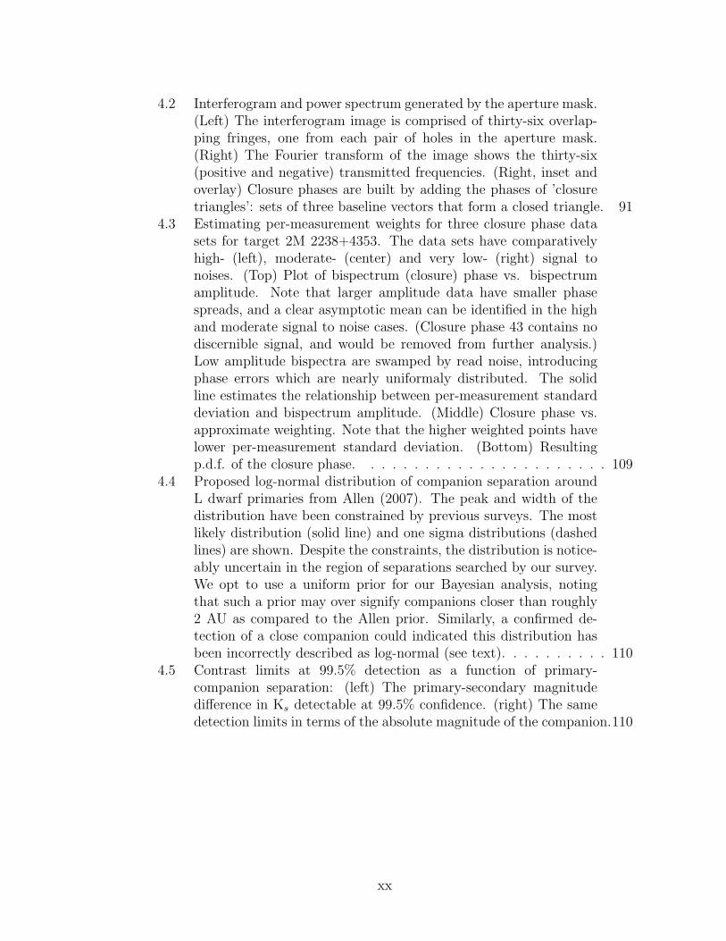
3.4 Monte Carlo simulation showing that all signal is virtually unre-coverable if phase noise is larger than about 150 degrees. Succes-sive averaging of a Gaussian variable usually reduces its measure-ment error by N−1/2; this is not the case for successive averagingof phasors when phase variance is large. Each data point showsthe measurement uncertainty of the phase of
∑N exp(ix), if x is
a mean-zero Gaussian variable with standard deviations rangingfrom 3 to 180 degrees. If the phase error of x is small, successiveaveraging leads to an N−1/2 improvement of error after N measure-ments. As the phase error approaches about 150 degrees, averagingis unable to recover that the mean phase is zero after any numberof measurements by this approach. . . . . . . . . . . . . . . . . . . 64
xviii
3.5 Closure phases increases the precision with which long-baselineFourier content can be measured. The x-axis is the set of eighty-four closure phases that can be extracted from a single image of thePalomar 9-hole mask. Each closure phase is constructed from setsof three baselines. Here we compare the variation of these baselinephases to the variation of the closure phase. Plotted in black are theclosure phases obtained from twenty aperture masking images; foreach closure phase, the individual baseline phases are overplotted(red, blue, green). As can be seen, the the closure phases (black)vary by about ∼ 3.3 degrees across the twenty separated exposures.Compare this to the individual baseline phases (red, blue, green),which vary by 30-35 degrees. This is a tenfold increase in fidelityby using closure phases. . . . . . . . . . . . . . . . . . . . . . . . . 68
3.6 Illustration of the phases as a function of baseline induced by a2:1 contrast binary separated by 150 mas using the Palomar 9-holeaperture mask. The phase signal of an unresolved single star isshown for comparison. (Middle) Showing the target phase as afunction of baseline, overplotted by the thirty-six spatial frequen-cies sampled by the Palomar mask. The uniform spatial frequency(or uv-coverage) coverage of the Palomar mask ensures sensitivityto companions at all separations and orientations. (Bottom) Show-ing the baseline-phase relation collapsed to one dimension. Thecompanion induces a phase offset of up to 30 degrees for manybaselines; with typical measurement precisions of a few degrees perclosure phase, this companion is readily detected at very high con-fidence. . . . . . . . . . . . . . . . . . . . . . . . . . . . . . . . . . 73
3.7 Determination of fit confidence with Monte Carlo is more conser-vative. Data is drawn from NRM observations of L-dwarf binary2M 0036+1806 (Bernat et al., 2010). The goodness-of-fit statistichere is ∆χ2=6.55 and is compared to a distribution generated fromfits to simulated single stars, resulting in a fit confidence of 96%(Monte Carlo). Notice that comparing this value to a χ2 distri-bution with three degrees of freedom (Analytic) results in a muchhigher confidence of fit. . . . . . . . . . . . . . . . . . . . . . . . . 80
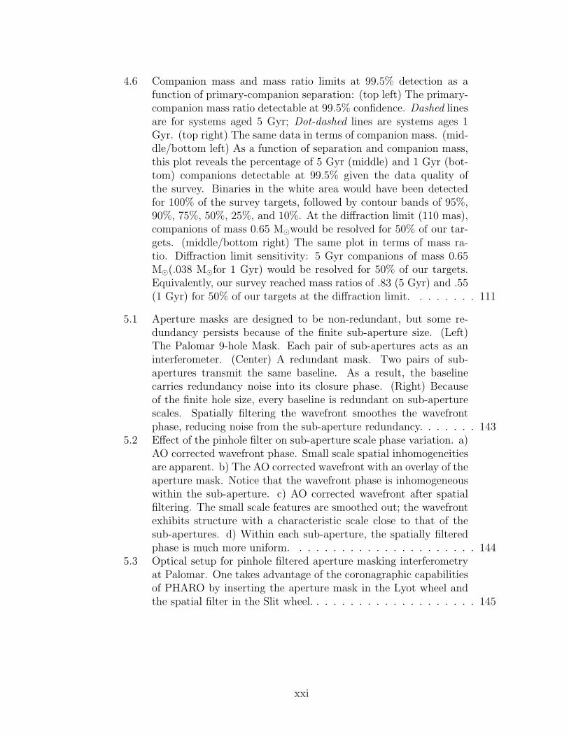
4.1 The aperture mask inserted at the Lyot Stop in the PHARO detec-tor. Insertion of the mask at this location is equivalent to maskingthe primary mirror. . . . . . . . . . . . . . . . . . . . . . . . . . . 91
xix
4.2 Interferogram and power spectrum generated by the aperture mask.(Left) The interferogram image is comprised of thirty-six overlap-ping fringes, one from each pair of holes in the aperture mask.(Right) The Fourier transform of the image shows the thirty-six(positive and negative) transmitted frequencies. (Right, inset andoverlay) Closure phases are built by adding the phases of ’closuretriangles’: sets of three baseline vectors that form a closed triangle. 91
4.3 Estimating per-measurement weights for three closure phase datasets for target 2M 2238+4353. The data sets have comparativelyhigh- (left), moderate- (center) and very low- (right) signal tonoises. (Top) Plot of bispectrum (closure) phase vs. bispectrumamplitude. Note that larger amplitude data have smaller phasespreads, and a clear asymptotic mean can be identified in the highand moderate signal to noise cases. (Closure phase 43 contains nodiscernible signal, and would be removed from further analysis.)Low amplitude bispectra are swamped by read noise, introducingphase errors which are nearly uniformaly distributed. The solidline estimates the relationship between per-measurement standarddeviation and bispectrum amplitude. (Middle) Closure phase vs.approximate weighting. Note that the higher weighted points havelower per-measurement standard deviation. (Bottom) Resultingp.d.f. of the closure phase. . . . . . . . . . . . . . . . . . . . . . . 109
4.4 Proposed log-normal distribution of companion separation aroundL dwarf primaries from Allen (2007). The peak and width of thedistribution have been constrained by previous surveys. The mostlikely distribution (solid line) and one sigma distributions (dashedlines) are shown. Despite the constraints, the distribution is notice-ably uncertain in the region of separations searched by our survey.We opt to use a uniform prior for our Bayesian analysis, notingthat such a prior may over signify companions closer than roughly2 AU as compared to the Allen prior. Similarly, a confirmed de-tection of a close companion could indicated this distribution hasbeen incorrectly described as log-normal (see text). . . . . . . . . . 110
4.5 Contrast limits at 99.5% detection as a function of primary-companion separation: (left) The primary-secondary magnitudedifference in Ks detectable at 99.5% confidence. (right) The samedetection limits in terms of the absolute magnitude of the companion.110
xx
4.6 Companion mass and mass ratio limits at 99.5% detection as afunction of primary-companion separation: (top left) The primary-companion mass ratio detectable at 99.5% confidence. Dashed linesare for systems aged 5 Gyr; Dot-dashed lines are systems ages 1Gyr. (top right) The same data in terms of companion mass. (mid-dle/bottom left) As a function of separation and companion mass,this plot reveals the percentage of 5 Gyr (middle) and 1 Gyr (bot-tom) companions detectable at 99.5% given the data quality ofthe survey. Binaries in the white area would have been detectedfor 100% of the survey targets, followed by contour bands of 95%,90%, 75%, 50%, 25%, and 10%. At the diffraction limit (110 mas),companions of mass 0.65 M�would be resolved for 50% of our tar-gets. (middle/bottom right) The same plot in terms of mass ra-tio. Diffraction limit sensitivity: 5 Gyr companions of mass 0.65M�(.038 M�for 1 Gyr) would be resolved for 50% of our targets.Equivalently, our survey reached mass ratios of .83 (5 Gyr) and .55(1 Gyr) for 50% of our targets at the diffraction limit. . . . . . . . 111
5.1 Aperture masks are designed to be non-redundant, but some re-dundancy persists because of the finite sub-aperture size. (Left)The Palomar 9-hole Mask. Each pair of sub-apertures acts as aninterferometer. (Center) A redundant mask. Two pairs of sub-apertures transmit the same baseline. As a result, the baselinecarries redundancy noise into its closure phase. (Right) Becauseof the finite hole size, every baseline is redundant on sub-aperturescales. Spatially filtering the wavefront smoothes the wavefrontphase, reducing noise from the sub-aperture redundancy. . . . . . . 143
5.2 Effect of the pinhole filter on sub-aperture scale phase variation. a)AO corrected wavefront phase. Small scale spatial inhomogeneitiesare apparent. b) The AO corrected wavefront with an overlay of theaperture mask. Notice that the wavefront phase is inhomogeneouswithin the sub-aperture. c) AO corrected wavefront after spatialfiltering. The small scale features are smoothed out; the wavefrontexhibits structure with a characteristic scale close to that of thesub-apertures. d) Within each sub-aperture, the spatially filteredphase is much more uniform. . . . . . . . . . . . . . . . . . . . . . 144
5.3 Optical setup for pinhole filtered aperture masking interferometryat Palomar. One takes advantage of the coronagraphic capabilitiesof PHARO by inserting the aperture mask in the Lyot wheel andthe spatial filter in the Slit wheel. . . . . . . . . . . . . . . . . . . . 145
xxi

5.4 Imaging An Unresolved Targets Through a Pinhole. The pointspread function of three targets is shown with a pinhole of size6λ/D overlaid. Square root contrast scaling is used to highlightthe truncated flux. (Left) The pinhole, located in an image plane,truncated the portion of electric field which forms the outer rings ofthe point spread function. In perfect seeing, the total flux blockedis very low. (Center) Wavefront errors dispel flux outward creat-ing a diffuse halo around the target. The blocked flux increases,and more power aliases back into sub-aperture scales, resulting inclosure phase errors. (Right) When asymmetrically truncated, thecenter of light shifts towards the pinhole center (black x). Eachcomponent of a binary is truncated differently, leading to errors inastrometry or contrast. . . . . . . . . . . . . . . . . . . . . . . . . 145
5.5 Effect of a Window Function. (Top Left) The aperture mask pro-duces a set of interference fringes beneath an envelope of size λ/dsub,as seen in this Palomar 9-hole masking image. The central peakhas been zeroed to highlight the envelope and outer rings. Theradius of the white ring is λ/dsub.(Bottom Left) The power spec-trum of the same interferogram, presented in units of baseline/Drather than spatial frequency. Each island of transmitted power(or splodge) is of size 2dsub. This is expected, as the transmissionfunction is related to the autocorrelation of the mask. (Top Right)Using a window function of characteristic HWHM λ/dsub (here, asuper-Gaussian) removes the interferogram wings and its associatedread and wavefront noise. (Bottom Right) The window functionproduces a convolution kernel of size λ/2HWHM. Notice that awindow function larger than 0.5 λ/dsub creates a kernel larger than2dsub and mixes neighboring splodges, adding redundancy noise.(see text) . . . . . . . . . . . . . . . . . . . . . . . . . . . . . . . . 146
5.6 The RMS fit residuals of simulated data (H-band, no read noise)with pinholes of various size, analyzed with (solid line) and without(dashed line) a window function. The horizontal line is the mea-surement level without any pinhole in place. The pinhole filter ismost effective within the range 11-14 λ/D. . . . . . . . . . . . . . 147
5.7 Misalignment of a single star within the pinhole introduces closurephase errors. (a) The Palomar 9-hole mask, overlaid with threeclosure triangles for which the misalignment errors are calculated.(b) Error due to misalignment at 1.6 µm (H band) as a function oftarget distance from the pinhole center. (Several azimuthal orien-tations are plotted for each separation.) (c) Closure phase errors at2.2 µm (Ks band), in which the pinhole is smaller. In both cases,errors in visibility amplitude errors below .005 for the same ranges. 155
xxii
5.8 Window functions reduce closure phase error from read noise.These curves, from top to bottom, display the reduction in RMSclosure phase error when read noise is 0% (top, solid), 0.2%, 0.4%,0.6%, 1.0%, and 5.0% (bottom, dotted) of the peak image inten-sity. The optimal window function is typically of size ∼ λ/dsub, or∼ 12λ/D for the Palomar aperture mask, with higher read noise fa-voring tighter window functions. Smaller window functions quicklyadd large amounts of redundancy noice. (See text.) Note: Evenwith no read noise (solid curve), a window function reduces closurephase errors, indicating that the window function provides an effectsimilar to spatially filtering the wavefront. . . . . . . . . . . . . . . 156
5.9 Curves showing the effectiveness of the window function as in Fig-ure 5.8, except the wavefront is static over an exposure. Mostnotably, a window function provides better spatial filtering whenthe wavefront is static (solid line). . . . . . . . . . . . . . . . . . . 157
5.10 Drops in flux transmission through the pinhole are driven bychanges in AO performance. The binary GJ 623 was resolved inKs using twenty five masking images through the pinhole. The im-ages which produced the best fitting closure phases (as measured byR.M.S. deviation from the model) also had the least flux blocked bythe mask. Poor correction displaces more flux into the outer haloof the PSF, which is then blocked by the pinhole. Poor correctionalso leads to larger closure phase errors. This trend is not causedby misalignment or movement of the target within the pinhole (seetext), but rather changes in AO correction. . . . . . . . . . . . . . 158
5.11 Closure phase standard deviation (scatter) is reduced and baselinevisibility amplitude is increased when observed through the pin-hole filter. Data points are drawn from observations of 26 singlestars. Horizontal lines are the median of the data (solid) and thesimulated experiment (dashed). (Top Row) Closure phase scatteris reduced by 10 and 19 percent in H and Ks band measurements,respectively. (Bottom Row) Visibility amplitude is increased by 14and 18 percent in H and Ks bands, respectively. In all cases, thesimulation (model) predicts a larger reduction in noise (see Discus-sion). . . . . . . . . . . . . . . . . . . . . . . . . . . . . . . . . . . 159
xxiii
6.1 Star-Planet Contrast of brown dwarfs and massive Jupiters (greentracks) orbiting a late-G star, plotted against anticipated P1640NRM contrast limits (black lines). Youthful brown dwarfs andexoplanets are bright enough to be detected by NRM on P1640and Gemini Planet Imager. Vertical lines (blue) plot the age ofknown, nearby moving groups. Note that planets of mass 6-9 MJ
are consistently detectable with the estimated performance usingextreme-AO and precision wavefront control (see text). A browndwarf of any mass can be detected most targets. . . . . . . . . . . 183
6.2 (Top) Histogram of visual magnitudes for all currently known mov-ing group objects observable from Gemini Observatory. Fifty-threetargets are V < 8.5 and ninety-one targets are V < 9.5. I bandmagnitudes are 0.5 lower (i.e., V-I=0.5) for these targets. Thesesets represent I < 8 and I < 9, respectively, in the AO sensingwavelength of the Palomar AO system. (Bottom) Histogram ofdistances for the 91 targets with I < 9. The median distance is 45pc, corresponding to physical separations of 1.8 - 7.2 AU for thePalomar NRM working angles. . . . . . . . . . . . . . . . . . . . . 184
A.1 The sparse, non-redundant aperture mask used for observations atthe Hale 200” Telescope at Palomar Observatory. Each pair ofsub-apertures acts as an interferometer of a unique baseline lengthand orientation. Overdrawn is one such baseline. The 9-hole maskproduces thirty-six baselines total; the point spread function of themask is a set of thirty-six overlapping fringes underneath a largeAiry envelope. . . . . . . . . . . . . . . . . . . . . . . . . . . . . . 201
xxiv
CHAPTER 1
PERSPECTIVE
1.1 Directly Imaging Faint Companions to Stars
At the present in 2011, this decade opens at the era of directly imaged exoplan-
ets. The successful detections of new planetary systems by transit and radial
velocity methods during the last decade have fueled remarkable new advances and
interest in high-contrast imaging. Whereas transit and radial velocity detections
of exoplanets tell us volumes about the bulk and statistical properties of plane-
tary systems, full characterization of individual planetary atmospheres awaits their
successful (spectroscopic) imaging, and the use of complex chemical and thermo-
dynamical models to interpret their atmospheres. As often stated in the literature,
this is a challenge of very high contrast imaging, and one in which the fundamental
limitations of which are also only recently being discovered.
The atmosphere introduces rapid phase variation into the incoming wavefront
which, even after suppression by adaptive optics (AO) systems, produces diffraction
effects which litter the image with bright speckles. The image noise is overwhelm-
ingly dominated by the movement and random fluctuation of speckles (Racine
et al., 1999); distinguishing true companions from bright speckles requires longer
observations than initially anticipated (e.g., Racine’s ’speckle tax’) dampening the
hopes of early, optimistic planet searches (e.g., Nakajima (1994)).
Speckles at close separations – those which inhibit high-angular resolution
searches – are much more nefarious. Speckles are not placed randomly, but are
preferentially pinned to the first and second Airy rings (Bloemhof et al., 2000,
1
2001; Sivaramakrishnan et al., 2003). Furthermore, the precise shape of the Airy
rings and pinned location of the speckles shift on timescales of tens of seconds to
tens of minutes (e.g., Hinkley et al. (2007)), driven by slowly varying instrumen-
tal wavefront errors. In recent years, the impact of these quasi-static wavefront
errors have been extensively explored, mostly in the pursuit of high-contrast coro-
nagraph observations Lafreniere et al. (2007). These wavefront errors evolve due
to temperature or pressure changes, mechanical flexures, guiding errors, changing
illumination of the primary mirror, or other phenomena (Marois et al., 2005, 2006).
Those originating from optical components located after the wavefront sensor can-
not be corrected by adaptive optics (named non-common path wavefront errors),
and give rise to quasi-static speckle behavior.
Quasi-static speckles present a particularly difficult challenge for high contrast
imaging: purely static speckles could be removed by calibration with a reference
star (i.e., treated as a non-ideal point spread function), but quasi-static speckles
evolve too quickly to calibrate and too slowly to effectively average out over even
hour long exposures (Hinkley et al., 2007). Quasi-static speckles dominate long
exposures within separations of 5-10 arcseconds at the Keck and Palomar Hale
Telescopes, and longer exposures do not yield any higher contrasts (Macintosh
et al., 2005; Metchev et al., 2003). My own investigation using the Palomar AO
system and PHARO instrument show intensity variations of as much as 10% the
peak flux over ten minute spans (2-5% on the second Airy ring), and pinned speck-
les that change locations irregularly (Figure 1.1). (Similar results were obtained
with PHARO by Bloemhof et al. (2000).)
Unequivocally, quasi-static speckles set the ultimate noise floor of high contrast
imaging, generating a slowly varying distribution of flux that can be mistaken for
2
faint companions.
Several techniques have been developed to differentiate and remove the quasi-
static speckles simultaneously with observation of the science target. Angular
Differential Imaging (ADI) employs multiple observation of the same target while
changing the rotation of the primary mirror on the sky (Marois et al., 2006);
the speckles move with the optical system rotation but target does not. Several
newly commissioned instruments aim to exploit the inherent dependence of speckle
behavior on wavelength (or polarization) by obtaining simultaneous images across
multiple wavelengths (or polarizations) (Marois et al., 2005; Lenzen et al., 2004;
Hinkley et al., 2009; Hinkley, 2009; Crepp et al., 2010). These include Project
1640 at Palomar (Hinkley et al., 2009), the Gemini Planet Imager (Macintosh
et al., 2008), and SPHERE on VLT (Beuzit et al., 2006) which use integral field
spectrographs for simultaneous chromatic imaging.
The work of this manuscript confronts the quasi-static imaging challenge us-
ing the technique of Non-Redundant Aperture Masking Interferometry (NRM , or
aperture masking). NRM provides a powerful, established method for obtaining
higher contrasts at diffraction-limit separations despite the atmospheric that pro-
duce speckles. Aperture masking employs a small metallic mask which transforms
the pupil into an ad-hoc interferometric array; utilizing the unique structure of the
transformed point spread function allows the construction of a dataset (i.e., clo-
sure phases, Jennison (1958); Lohmann et al. (1983); Baldwin et al. (1986); Haniff
et al. (1987); Readhead et al. (1988); Cornwell (1989)) which retains the fidelity of
high-resolution spatial information while discarding the effect of many wavefront
error sources.
The heritage of aperture masking extends back to short-exposure speckle inter-
3
AO Direct Image (T= 18.6s)
-300 -200 -100 0 100 200 300Offset From Primary (milliarcseconds)
-300
-200
-100
0
100
200
300
Off
se
t F
rom
Prim
ary
(m
illia
rcse
co
nd
s)
AO Direct Image (T= 37.2s)
-300 -200 -100 0 100 200 300Offset From Primary (milliarcseconds)
-300
-200
-100
0
100
200
300
Off
se
t F
rom
Prim
ary
(m
illia
rcse
co
nd
s)
AO Direct Image (T= 80.6s)
-300 -200 -100 0 100 200 300Offset From Primary (milliarcseconds)
-300
-200
-100
0
100
200
300
Off
se
t F
rom
Prim
ary
(m
illia
rcse
co
nd
s)
AO Direct Image (T= 86.8s)
-300 -200 -100 0 100 200 300Offset From Primary (milliarcseconds)
-300
-200
-100
0
100
200
300
Off
se
t F
rom
Prim
ary
(m
illia
rcse
co
nd
s)
AO Direct Image (T=136.4s)
-300 -200 -100 0 100 200 300Offset From Primary (milliarcseconds)
-300
-200
-100
0
100
200
300
Off
se
t F
rom
Prim
ary
(m
illia
rcse
co
nd
s)
AO Direct Image (T=285.2s)
-300 -200 -100 0 100 200 300Offset From Primary (milliarcseconds)
-300
-200
-100
0
100
200
300
Off
se
t F
rom
Prim
ary
(m
illia
rcse
co
nd
s)
AO Direct Image (T=669.6s)
-300 -200 -100 0 100 200 300Offset From Primary (milliarcseconds)
-300
-200
-100
0
100
200
300
Off
se
t F
rom
Prim
ary
(m
illia
rcse
co
nd
s)
AO Direct Image (T=700.6s)
-300 -200 -100 0 100 200 300Offset From Primary (milliarcseconds)
-300
-200
-100
0
100
200
300
Off
se
t F
rom
Prim
ary
(m
illia
rcse
co
nd
s)
AO Direct Image (T=762.6s)
-300 -200 -100 0 100 200 300Offset From Primary (milliarcseconds)
-300
-200
-100
0
100
200
300
Off
se
t F
rom
Prim
ary
(m
illia
rcse
co
nd
s)
Figure 1.1: Close-up of the diffraction core and first and second Airy rings of 6second exposures of HIP 52942, taken with the Palomar AO system and PHAROinstrument. The field of view is 600 mas. Contours are peak intensity dividedby 1.05, 1.18, 1.33, 2., 2.5, 3.33, 5., 10., 20., and 50. Each row contains threeimages taken roughly ten seconds apart. The middle and bottom rows have setsof images taken 1 and 10 minutes after the first row, respectively. The tendency ofspeckles to ’pin’ to the Airy rings is readily apparent, as well as a three-fold andfour-fold symmetry of the speckle locations on the first Airy ring which evolves onminute timescales. (For instance, between the first and second image of the firstrow.) These produce flux variations as much as 10% of the peak (seventh contour).Variations on the second Airy ring of as much as 2-5% are also observed. Thesequasi-static speckles limit the image contrast.
4
ferometry and non-redundant experiments (Weigelt, 1977; Roddier, 1986; Naka-
jima, 1988; Tuthill et al., 2000). The development of adaptive optics has altered
the requirements of non-redundancy and short exposure times, but the technique
remains highly effective for mitigating quasi-static instrumental wavefront errors.
Importantly, the technique provides a method for mitigating or calibrating out the
effect of quasi-static wavefront errors from a single image, i.e., before quasi-static
wavefront errors evolve. These features allow aperture masking to reach much
higher contrast in routine observing and a much lower noise floor, particularly at
separations close to the primary and at the diffraction limit (Figure 1.2).
Aperture masking with adaptive optics is well-established for resolving stellar
companions within the formal diffraction limit (down to 0.5λ/D) and at high
contrasts (200:1 at λ/D)(Tuthill et al., 2000; Lloyd et al., 2006; Ireland et al.,
2008; Martinache et al., 2007). This range of high-resolution and high-contrast
make aperture masking ideal for close companion searches. Binaries resolved with
aperture masking also have higher precision photometry and relative astrometry.
The ultimate limitation of the NRM technique, although certainly due to quasi-
static wavefront errors which cannot be mitigated by closure phases, has not been
well-explored before the start of this body of work. The relationship between wave-
front errors, AO performance, and closure phase errors will be critical for designing
NRM experiments optimized for new systems, and ultimately, reaching planetary
contrasts. In particular, their interplay at high-strehl ratio correction or with inte-
gral field spectrographs is completely unexplored. These various techniques aiming
to solve the quasi-static imaging problem are complementary. Given that the exo-
planet dedicated instruments (Project 1640, Gemini Planet Imager, and SPHERE)
are equipped with aperture masks, now is the time to lay the groundwork for fu-
5

Figure 1.2: Comparison of imaging techniques in infrared H Band (Strehl ∼20%) at Palomar Hale 200” Telescope. Aperture Masking (red) routinely achieves∆H∼5.5 magnitudes (150:1) at the diffraction limit, much better than direct imag-ing alone (black). Coronagraphy (blue), although capable of providing very highcontrast is obscured at close separations by its Lyot stop. High contrast at closeseparations is crucial for the detection of brown dwarfs for dynamical mass mea-surements. An M-Brown dwarf binary (Contrast ∼ 4.0-5.0 magnitudes, 80-100:1)cannot be detected by direct imaging at a separation closer than about 3 λ/D; thesystem would have a period of at least 9 years. Aperture Masking can detect thesebinaries over a more expansive range, and with much shorter periods. Companionsdetected by coronagraphy are rarely able to provide dynamical masses.
6
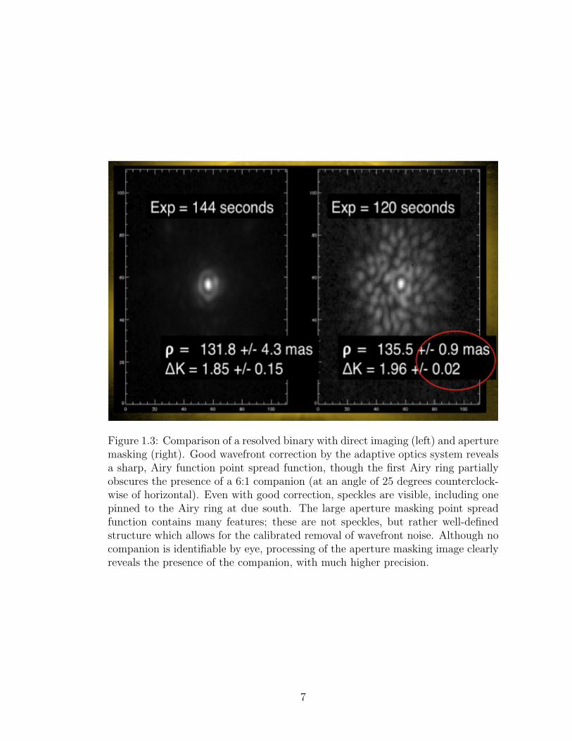
Figure 1.3: Comparison of a resolved binary with direct imaging (left) and aperturemasking (right). Good wavefront correction by the adaptive optics system revealsa sharp, Airy function point spread function, though the first Airy ring partiallyobscures the presence of a 6:1 companion (at an angle of 25 degrees counterclock-wise of horizontal). Even with good correction, speckles are visible, including onepinned to the Airy ring at due south. The large aperture masking point spreadfunction contains many features; these are not speckles, but rather well-definedstructure which allows for the calibrated removal of wavefront noise. Although nocompanion is identifiable by eye, processing of the aperture masking image clearlyreveals the presence of the companion, with much higher precision.
7
ture NRM experiments aimed at planet detection. Among the scientific potential of
NRM exoplanet imaging is the mass measurement of exoplanets, the full character-
ization of imaged planetary systems (including upcoming coronagraphic surveys,
and e.g., Hinkley et al. (2011)), and exoplanets formed in situ by core accretion
(Kraus et al., 2009).
1.2 Brown Dwarfs as Massive Exoplanet Analogs
The exoplanet’s more massive cousins in the substellar regime – brown dwarfs –
still present many outstanding questions regarding their atmospheres, underlying
physical characteristics, and formation processes. It is, perhaps, ironic that the
first observational discoveries of these new objects were announced nearly simulta-
neously at the Cool Stars IX meeting in 1995: the first direct image of a confirmed
brown dwarf (Nakajima et al., 1995; Oppenheimer et al., 1995), GJ 229B; and the
first radial velocity discovery of an extrasolar Jupiter-mass planet (Mayor, 1995).
While brown dwarfs and exoplanets form in separate environments, they span
similar ranges of mass and composition; much of the fundamental core of our under-
standing of the evolution, structure, and atmospheres of giant Jupiter-mass planets
derives directly from extensions of brown dwarf models (Burrows et al., 2001). The
natural physical and observational similarities between dim, cool brown dwarfs
and much dimmer Jupiter-mass exoplanets provide brown dwarfs as an excellent
laboratory to understand the underlying physical development and observational
characteristics of Jupiter-class planets. This will remain true for the foreseeable
future even after direct imaging searches begin to reveal exoplanets in droves; most
of the physical insights drawn out of exoplanet images and low resolution spectra
8

will be extracted from evolution and atmospheric models. One can perhaps view
the previous two decades of observational challenges to brown dwarf imaging as a
template for the era of directly imaged planets, while recognizing that successful,
concurrent observations of brown dwarfs directly add to our understanding of both
classes of objects.
The formation of a brown dwarf begins in the same protostellar dust regions
that produce stars, yet an unknown process curbs mass accretion before the brown
dwarf has enough mass to raise its core temperatures to the levels necessary to
ignite hydrogen fusion (Kumar, 1963; Hayashi & Nakano, 1963). Instead, brown
dwarfs support themselves against gravitational collapse by a combination of elec-
tron degeneracy and Coulomb pressure. With no fusion energy production, brown
dwarfs shine by converting their gravitational potential energy into luminosity, a
process which alters the temperature and structure of brown dwarfs as they age. In
this regard, brown dwarfs and Jupiter-mass planets share common mechanisms for
structural morphology and evolution. Theoretical models estimate the bifurcation
between stars and brown dwarfs to occur at about 0.072-0.075 solar masses (M�)
for solar composition, or 75-80 times the mass of Jupiter (MJ) 1. At formation, the
most massive brown dwarfs reach temperatures are high as about 3200 K, but cool
below 2000 K by one billion years. The temperature of a brown dwarfs depend on
its mass and age, but span about 500-2000 K at one billion years and cooling as
far as 300-1300 K by ten billion years.
Yet astronomy is a visual science: nearly everything we know about the uni-
verse has been deduced from the light which shines down upon our telescopes.
1No clear physical distinction can be made between brown dwarfs and planets, though themonicker planet is generally reserved for objects which are presumed to have formed in the debrisdisks of stars. Other authors chose a mass cutoff at 13MJ , for brown dwarfs above this massbriefly ignite the fusion of primordial deuterium. The latter definition assures that planets neverengage in fusion. This work will chose for the former, formation-based definition.
9

And connecting the photometric and spectral properties of those distant pinpoints
of light to physical parameters such as mass, radius, age, composition, and tem-
perature is the fundamental challenge of stellar and substellar astrophysics. The
development of astrophysical models of stars stands as one of the successes of the
twentieth century: knowing the mass and metallicity of a star reveals the entire
nature of that star including its spectral features, internal structural dynamics,
and ultimate evolutionary future. No complete, robust, and empirically tested
model exists for brown dwarfs or planets at this time.
It is more than the intrinsic faintness of brown dwarfs that makes them harder
to observe and model. It is that brown dwarfs cool and evolve with age (a notori-
ously difficult parameter to measure precisely), adding an extra dimension to the
development of models which connect observable features to fundamental physical
parameters (i.e., mass, age, and composition).
In the two decades since the detection of the first brown dwarf, hundreds of iso-
lated brown dwarfs have been imaged and spectra have been obtained by large scale
surveys (such as 2MASS, Dahn et al. (2002)). These spectra have permitted the
advancement of atmospheric models which relate the observed spectral features to
properties of the atmosphere: surface temperature, molecular chemistry, and dust
grain mechanics. These models convey a rich photochemistry of molecules and
metallic dust forming in the atmospheres of brown dwarfs. Thousands of molecu-
lar species can be formed, and these molecules undergo interactions with radiation
across a wide spectrum of infrared and mid-infrared wavelengths. Metallic dust
forms clouds in the atmospheres of warm brown dwarfs that deplete metals from
the atmosphere and drive chemical equilibria; at cooler temperatures, these dust
grains rain out of the atmosphere. Both factors complicate the detailed modeling
10
of brown dwarf atmospheres in a way different than stars. Despite the numerous
successes, state-of-the-art models lack opacity characterization of numerous chem-
ical compounds at the pressures and temperatures of brown dwarfs and require
finely tuned parameters to seed rainout of dust grains as brown dwarfs cool. More
diverse empirical constraints are required to move these models forward.
But fundamental to the nature of brown dwarfs is their cooling through their
lifetime, and understanding the evolution of a brown dwarf with age is a formidable
task in its own right. Evolution models describe the internal structure, total lumi-
nosity output, radius, and temperature of a brown dwarf of a given mass and age
(and, to a lesser degree, composition). In concert with atmospheric models, one
has the basis for a complete model of brown dwarfs. The optical properties of the
atmosphere necessarily affect the evolution of the brown dwarfs by regulating the
bulk luminosity output, but evolution models are nonetheless relatively insensitive
to the specific details of atmosphere models. Independently testing brown dwarf
evolution models requires the measurement of masses, ages, and/or temperatures,
in addition to photometry.
Brown dwarf binary systems serve as an excellent laboratory for testing evo-
lution models. Tracking the system orbit provides measurement of (the sys-
tem) mass; combined with accurate photometry (and hence total luminosity, c.f.
Golimowski et al. (2004)) one has a critical data to empirically test evolution mod-
els (Liu et al., 2008). Observationally, detecting brown dwarf companions suitable
for dynamical masses requires imaging with high contrast and angular separations
close to the primary.
As discussed in the previous subsection, the technique of Non-Redundant Aper-
ture Masking Interferometry provides a powerful, well-established method for ob-
11

taining high-contrast at very close angular separations. Binaries resolved with
NRM also obtain higher precision photometry and relative astrometry, and dy-
namical masses up to an order of magnitude more precise (Figure 1.3).
Developing the technique of NRM on current and upcoming instruments will
be invaluable for obtaining high precision mass measurements of brown dwarfs and
giant exoplanets to advance evolution models.
1.3 The Organization of This Manuscript
These considerations have motivated the research presented within this disser-
tation. Chapter 2 continues an overview of the current state of brown dwarf
atmosphere and evolution models, and describes the challenges confronting the
detection of brown dwarf binaries for dynamical mass measurements. Chapter 3
introduces Non-Redundancy Aperture Masking Interferometry (NRM), focusing
on the difference between its application with and without adaptive optics and
its relevance to resolving binaries. The chapter also includes a general purpose
Monte Carlo simulation for determining the statistical significance of NRM de-
tections. Chapter 5 presents previously published results of an NRM search using
Laser Guide Star Adaptive Optics to detect companions to very low mass stars and
brown dwarfs. The survey detected four candidate brown dwarf binaries at low to
moderate confidence with projected physical separations favorable for dynamical
mass measurements. Chapter 6 presents unpublished results of an experiment to
increase the high contrast capabilities of aperture masking by spatially filtering
the science wavefront. A detailed analytical description of the spatial structure
of closure phase redundancy noise is also presented. Chapter 7 synthesizes the
12
results of this research and emphasizes their place in the ongoing developments of
this field. The impact of this work for future high-contrast infrared imaging and
for the study of brown dwarfs and exoplanets is discussed.
Dear Jamie, Ivan, Ira, Bruce, and Jeevak,
I am very happy to present to you the final draft of my dissertation. Upon
your approval, I will submit this to the graduate school.
I would like to thank all of you for your time and effort these last several
months, and for the guidance you have provided to me.
Sincerely, David Bernat
13

CHAPTER 2
BROWN DWARFS
2.1 How does one identify a brown dwarf?
The early pursuits for brown dwarf were marked by spectroscopic searches for
objects which could bridge the gap between the lowest known mass stars either
just above or straddling the hydrogen burning mass limit (late-type M dwarfs,
Teff ∼2600K) and the spectrum of Jupiter, marked most notably by deep methane
bands in the infrared (Teff ∼200K). The dominant feature of the lowest mass stars
are strong VO and TiO bands in the optical red.
Kirkpatrick (1992) identified GD 165B as an object much redder than the
lowest mass stars and lacking VO and TiO, with unidentified absorption features
but no methane absorption. Despite the lack of methane, the unique appearance
of its spectrum and extreme red color suggested that GD 165B ought be classified
beyond the Morgan-Keenan OBAFGKM spectral classifications (Morgan et al.,
1943), and proposed as a candidate brown dwarf. Without adequate models to
interpret the unidentified absorption features, the temperature was estimated to be
∼2200 K from total luminosity. Later spectral analysis and atmospheric modeling
of GD 165B identified features of metallic hydrides, and confirmed a substellar
temperature of (Teff ∼ 1900K, Kirkpatrick et al. (1999)).
The successful confirmation of the first brown dwarf followed the detection of
Gl 229B (Nakajima, 1994; Oppenheimer et al., 1995). The spectral analysis showed
strong absorption of methane and water, similar to that of Jupiter. Moreso, almost
all of the carbon was found in the form of methane rather than CO, offering an
14
independent estimation of its temperature based on purely chemical equilibrium
considerations (Tsuji, 1995)(Teff ∼900 K, Oppenheimer et al. (1998)).
The discovery of these objects provoked the establishment of two new spectral
types, L and T (Kirkpatrick et al., 1999), beyond the Morgan-Keenan OBAFGKM
spectral classification (Morgan et al., 1943), with GD 165B and Gl 229B as the
prototype members, respectively. Their discovery also led to quickly developing
advances in the brown dwarf atmospheric models.
Most notable of the early discoveries into the brown dwarf atmospheres is the
role metallic dust in the photosphere plays in shaping the spectra. Jones (1997)
demonstrated that dust grains (mostly iron and magnesium silicates) begin forming
in the atmospheres of the coolest stars, as well as GD 165B. Surprisingly, the
spectrum of Gl 229B is not consistent with a dusty atmosphere (Oppenheimer
et al., 1995).
For objects like GD 165B (L Dwarfs), dust grains drive the spectral features, in
particular the absence of TiO and VO as these oxides are absorbed into micron and
centamicron sized silicate grains (Kirkpatrick et al., 1999). This also allows the rise
in prominence of the metallic hydrides Tsuji (1995). The size of dust grains that
form is a function of temperature, pressure, and the particular chemical equilibrium
of each species under consideration (Grossman (1972), and described elsewhere in
Leggett et al. (1998); Allard et al. (2000)). These dust grains provide their own
opacity (Alexander & Ferguson, 1994), but the predominant overall effect of dusty
grains on opacity is by altering the composition of the photosphere gas (Lunine
et al., 1989).
The transition from CO to methane as the dominant carbon feature marks the
15
boundary between L and T dwarfs, and occurs over a narrow range of temperatures:
one expected equal parts CO and methane at about 1400 K, a factor of ten less
at 1250 K, and virtually no CO at 900 K (Marley et al., 1996). Furthermore,
the spectra and photometric colors are not consistent with dusty atmospheres,
indicating that dust clouds grow thicker as temperatures cool through the L dwarf
class but condense and ”rain out” near the onset of the T dwarf class. This allows
for the onset of non-metal absorbers, such as methane and water, in the spectra of
T dwarf (Allard et al., 2003). The dominance of water opacity in the atmosphere
of cool brown dwarfs forces flux emission to increase between the classic telluric
bands which define the infrared bands; this results is dramatically enhanced J and
H band (1.2µm and 1.6µm) fluxes relative to blackbody. (A similar enhancement in
M band occurs for even cooler dwarfs. (Burrows et al., 1997)). This enhancement
occurs in Ks band (2.2 µm) as well, but less so due to absorption by H2 and
methane, driving infrared colors not redder but bluer with decreasing temperature
(Leggett et al., 1998) (Figure 2.1).
2.2 The Current State of Brown Dwarf Atmosphere and
Evolution Models
The discovery of GD 165B and Gl 229B and the classification of L and T dwarfs
has allowed the development of models describing brown dwarf atmospheres and
their evolution in tandem with empirically derived relations.
Spectra of hundreds of L dwarfs and more than sixty T dwarfs have been
classified spectroscopically and photometrically (Cruz et al., 2003; Knapp et al.,
2004; Golimowski et al., 2004). Both infrared and optical spectral features and
16

Figure 2.1: Color-magnitude diagrams of substellar objects plotted against mod-eled atmospheres and blackbody curves. (Left) Absolute J v. J-K color magnitudediagram. Curves indicate theoretical isochrones for substellar objects at ages of0.5, 1.0, and 5.0 Gyr through a range of masses using the brown dwarf models ofBurrows et al. (1997) and their blackbody counterpart. The difference betweenblackbody colors and model colors is immediately apparent. The prototype Tdwarf, Gl 229B, and prototype L dwarf, GD 165B, are plotted for comparison.Notice that the L dwarf does not show an indication of particularly bluer-than-blackbody colors. (Right) Absolute J v. J-H color magnitude diagram. Figurefrom Burrows et al. (1997)
17
colors have been used to define subtypes from L1 through T9, all of which supply
consistent empirical tests of atmospheric models across the entire span of brown
dwarfs (Golimowski et al., 2004). These atmospheric models relate the photomet-
ric characteristics of a brown dwarf to its effective temperature (Teff ) and total
luminosity, as effective temperature is the primary driver of atmospheric chemistry,
with gravity and metallicity playing lesser roles (Burrows et al., 2006)
Empirical and semi-empirical relations have also been created which relate
total luminosity, effective temperature, spectral type, and infrared photometry.
Golimowski et al. (2004) has derived bolometric corrections for converting infrared
photometry to total luminosity, Lbol, using flux-calibrated optical and infrared
spectra from several dozen brown dwarfs. This spectral type-luminosity relation
has been show to provide more accurate estimations of total luminosity then fitting
atmospheric models to broad band photometry Konopacky et al. (2010) and is
purely empirical.
Total luminosity is also related to effective temperature:
Lbol = σ(4πR2)T 4eff . (2.1)
By making model-dependent assumptions of radius (Burrows et al., 1997;
Chabrier et al., 2000), Golimowski et al. (2004) also derived effective temperature
as a function of spectral type. These indicate the temperature ranges of L dwarfs
(1400 K. Teff .2200 K), and T dwarfs (400K. Teff .1300K), also showing
plateau of temperature between L7 and T4.5 (the so-called L/T Transition). This
plateau of temperature is consistent with the chemical analysis by Marley et al.
(1996) for Gl 229B indicating the sensitivity to temperature of the CO to methane
transition. Additional analysis of changes in infrared colors across this transition
are consistent with the onset of methane occurring with little temperature change,
18
but significant opacity changes in the near infrared, i.e., the condensation of dust
out of the photosphere.
Likewise, Cruz et al. (2003) derived empirical relations between J band (1.2
µm) photometry and spectral type. Knapp et al. (2004) derived empirical relations
between infrared photometry and spectral type using several dozen brown dwarf
spectra ranging down to T9.
Currently, two suites of brown dwarf atmosphere and evolution models are
widely used.
The set of models by Baraffe et al. (1998, 2003) and Chabrier et al. (2000)
(sometimes referred to collectively as the LYON models) treat L and T dwarfs
individually. The set of models appropriate for L dwarfs (the DUSTY model) as-
sumes dust grain clouds form (in chemical equilibrium) and affect opacity by the
scatter and absorption of flux, as well as by depleting the metallic and dust-forming
elements from the photospheric gas. The second set of models appropriate for T
dwarfs (the COND models) also assumes that dust grains forms, but that these
grains large enough to condense out and only affect opacity by their depletion of
metallic and dust forming elements. Neither of these models include any mech-
anism to drive grain growth and thus neither handle well brown dwarfs near the
L-T transition. Likewise, out of equilibrium chemical species are not included.
Chabrier et al. (2000) stressed that although the variations in the treatment
of dust could provoke large photometric and spectral changes, this had very little
effect on the overall cooling rate used by evolution models. In other words, one
need not derive evolution cooling curves for each set of atmospheric models (i.e.,
cooling curves are universal), and evolution models are fairly independent on the
19
finer details of atmospheric models (to about 10% in Teff and 25% in Lbol at the
extremes).
An alternative set of models by (Burrows et al., 2001) calculates the size of
dust grains, their distribution, and cloud sizes as driven by vapor pressure levels
within the atmosphere, following the model of Lunine et al. (1989). As such, there
is no need to distinguish between dusty L dwarfs and depleted T dwarfs, as this
is handled innately by the model; these models are sometimes referred to as the
PHOENIX/TUCSON models.
Atmosphere Models
Linking the observed features of the brown dwarf spectra to the underlying physical
chemistry in the photosphere is the fundamental aim of atmospheric chemistry.
The importance of obtaining accurate photometry across multiple wavebands and
spectra of brown dwarfs were recognized early as the fundamental limitation to
advancing the theory of brown dwarf atmospheres Stevenson (1986), and remain
one of the most important considerations still (Konopacky et al., 2010; Dupuy
et al., 2010).
Most of the trends and characteristics are understood in terms of general chem-
istry (Burrows & Sharp, 1999) which have put a premium on the calculation and
inclusion of accurate molecular opacities. However, the most difficult challenge
for the advance of atmospheric models is the accurate incorporation of a natural
mechanism for the formation of dust grains (calcium aluminates, silicates, and
iron) (Burrows et al., 2005). While a robust mechanism for grain condensation has
not yet been formed, more recent models suggest that changes is surface gravity
and metallicity, in addition to temperature, play an important role for driving the
20
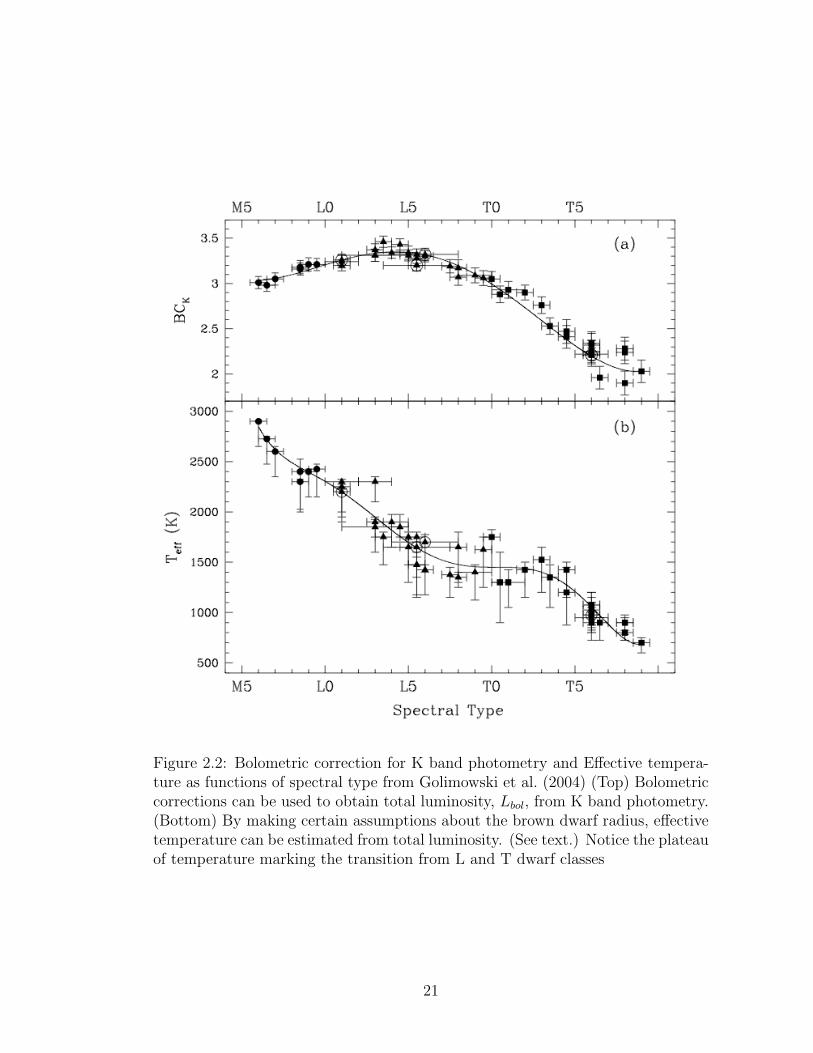
Figure 2.2: Bolometric correction for K band photometry and Effective tempera-ture as functions of spectral type from Golimowski et al. (2004) (Top) Bolometriccorrections can be used to obtain total luminosity, Lbol, from K band photometry.(Bottom) By making certain assumptions about the brown dwarf radius, effectivetemperature can be estimated from total luminosity. (See text.) Notice the plateauof temperature marking the transition from L and T dwarf classes
21

effect (Burrows et al., 2006).
Figure 2.3 shows the progression of infrared photometry through spectral type
for solar mass stars, low mass stars, and brown dwarfs. Solar mass infrared pho-
tometry use the empirical mass-luminosity relations of Henry & McCarthy (1993).
Low mass stars (M0 and later) and brown dwarfs use the photometry of Baraffe
et al. (2003) and the spectral type-MJ relation of Cruz et al. (2003). The infrared
photometry of a blackbody is drawn for comparison; the infrared flux brightening
of dusty stars (M6 and later) and brown dwarfs is readily apparent.
Evolution Models
As stated previously, brown dwarfs shine by converting their gravitational energy
into luminosity and slowly cool with age. In other words, the internal structure
(i.e., radius, convention zone, etc.), temperature, and luminosity, of a brown dwarf
of a particular mass evolves with time.
The evolution with age of total luminosity and effective temperature of very low
mass stars, brown dwarfs, and planets through the lower spectral types are shown
in Figures 2.4 and 2.5 using the evolution models of Burrows et al. (2001). Cooling
during evolution results from the bulk luminosity output of brown dwarfs, and
therefore is not particularly sensitive to the details of the atmospheric model used
to describe the specific wavelengths of radiation emitted. These evolution curves
can therefore be viewed as nearly universal and independent from atmospheric
models.
Brown dwarfs form quite warm and bright (Teff ∼ 2500-3200 K), and at tem-
peratures on par with low-mass main sequence stars. This highlights the fundamen-
22

G0 G5 K0 K5 M0 M5 L0 L5 T0Spectral Type
20
15
10
5
0
Absolu
te M
agnitude
6000 5600 5200 4400 3600 2800 2000 1500 Effective Temperature (K)
Max BDMass ~5 Gyr
Max BDMass ~1 Gyr
Max BDMass ~100 Myr
Min BDMass ~100 Myr
Infrared Photometry of Low Mass Stars
Figure 2.3: Infrared photometry of low mass stars as a function of effective tem-perature. Photometric colors are primarily a function of effective temperatureand predominantly dependent on the physical chemistry of the brown dwarf atmo-spheres. In the absence of spectra, broadband photometric colors are a proxy forspectral type and temperature. Low mass curves (M0 and later) use photometryof Baraffe et al. (2003) and the spectral type-MJ relation of Cruz et al. (2003).High mass curves use the mass-luminosity relations of Henry & McCarthy (1993).The infrared photometry of a blackbody is drawn for comparison; the infrared fluxbrightening of dusty stars (M6 and later) and brown dwarfs is readily apparent.
23
tal problem of using spectral type (or effective temperature) alone as a predictor of
brown dwarf mass. That is, an object classified as a late-M dwarf may be either a
young brown dwarf or an old-main sequence star. To accurately access the brown
dwarf mass, luminosity and age are necessary. In general regarding total luminos-
ity, effective temperature, mass, and age, evolution models can be used with any
two quantities to calculate the remaining two.
From these figures, it is clear that the lowest-mass hydrogen burning stars are
in fact early L dwarfs, and brown dwarfs of all masses begin as M dwarfs for the
first hundred million years of their life. But as expected from earlier investigations,
brown dwarfs evolve predominantly through the L (1400 K. Teff .2200 K) and
T (400K. Teff .1300K) spectral types.
The minimum hydrogen-burning mass is a clear demarcation between brown
dwarfs and stars at 0.072-0.075 M�, below which hydrogen fusion is not ignited.
However, brown dwarfs between 13 and 80 MJ do undergo a brief period when
young in which they fuse primordial deuterium. This onset of deuterium fusion
can be seen in the brief shoulder of constant luminosity in tracks of Figure 2.4
before brown dwarfs reach an age of 50 million years. Because objects less massive
than 13 MJ never reach deuterium fusing temperatures, this is occasionally used
to distinguish between brown dwarfs and planets.
Brown dwarfs more massive than 65 MJ also undergo a brief period of primor-
dial lithium fusion at an age of about 10 million years. This provides one method
for placing an upper limit on the mass of an observed brown dwarf: the presence
of lithium in the brown dwarf spectrum places the mass at below 65 MJ (Rebolo
et al., 1992)
24
Evolution models have limited effectiveness for brown dwarfs (and particularly
massive exoplanets) at ages of less than tens of millions of years, as the specific
characteristics of objects this young are still quite sensitive to the conditions of
formation (Marley, 2007; Fortney et al., 2008). Most strikingly, models predict the
total luminosity of young objects can span a factor of hundreds or thousands, de-
pending on the method by which brown dwarfs and exoplanets expel their entropy
during formation (i.e., ’hot start’ versus ’cold start’). The specific formation mech-
anism can affect the observable properties of these objects out to an age of one
billion years, depending on the mass of the object. Importantly, evolution models
are least well constrained empirically at young ages, and the majority of directly
imaged exoplanets will be youthful (because they are brighter). This speaks to
the immediate need for empirical constraints on brown dwarf evolution models at
young ages.
Because evolution models provide the mass-luminosity-age relation for brown
dwarfs, one only needs two of the three to calculate the third. In particular, a
measurement of the brown dwarf mass combined with luminosity (or photometry)
allows one to place a constraint on the brown dwarf age. Constraints on age are
more effective for young brown dwarfs, for which luminosity tracks are more widely
spaced (See Figure 2.4).
Using the evolution model of Baraffe et al. (2003), we can explore the mass-
temperature-age relation of very low mass stars and brown dwarfs. Figure 2.6
shows the relationship between mass and effective temperature for stellar and sub-
stellar objects for three isochrones (ages of 100 million years, 1 and 5 billion years).
As can be seen, young (∼ 100 million years old) brown dwarfs span temperatures
of 1500-2500 K, cooling by as much as 1500 K over their lifetime. The oldest,
25
lowest mass brown dwarfs reach temperatures as low as 400 K. High mass curves
use the empirical mass-luminosity relations of Henry & McCarthy (1993).
Using the evolution and atmospheric models of Baraffe et al. (2003) we can
explore the mass-luminosity-age relation of very low mass stars and brown dwarfs.
Figure 2.7 shows the relationship between mass and infrared photometry for stellar
and substellar objects of the same isochrones are Figure 2.6. Despite the flux
enhancement in the infrared, brown dwarfs are still much fainter than more massive
objects in these wavebands. Eight magnitudes (1500:1 flux ratio) separate solar
mass stars and the most massive brown dwarfs at an age of 1 billion years. This
flux ratio improves at younger ages, but remains larger than 6 magnitudes (250:1)
for younger objects. The onset of the T dwarf spectral class can be inferred from
these curves by locating the point at which J band fluxes grows brighter than K
band, at a mass of about 0.030 M� at 1 billion years.
2.3 Using Mass Measurements to Test Evolution Models
Brown dwarf atmospheric models are capable of reproducing the photometry and
spectral features across the span of brown dwarf spectral types. As shown in Figure
2.2, these spectral types can be well characterized by their effective temperature
and total luminosity. Spectra of hundreds of isolated brown dwarfs have been
instrumental in advancing these models to their current state.
Brown dwarf evolution models relate the physical parameters of mass, age, and
radius, to total luminosity and effective temperature, which can then be used by
atmospheric models to determine photometry or spectra. Yet, the fundamental
difficulty of measuring the mass, age, and/or radius of a brown dwarf has limited
26
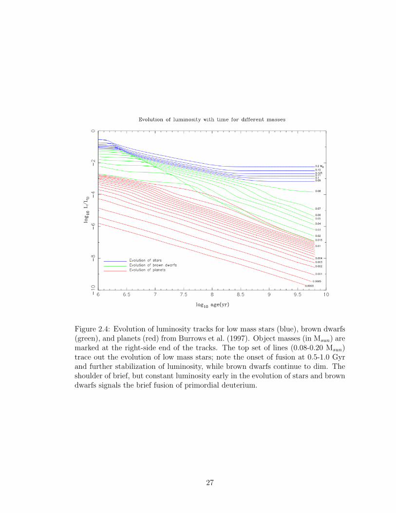
Figure 2.4: Evolution of luminosity tracks for low mass stars (blue), brown dwarfs(green), and planets (red) from Burrows et al. (1997). Object masses (in Msun) aremarked at the right-side end of the tracks. The top set of lines (0.08-0.20 Msun)trace out the evolution of low mass stars; note the onset of fusion at 0.5-1.0 Gyrand further stabilization of luminosity, while brown dwarfs continue to dim. Theshoulder of brief, but constant luminosity early in the evolution of stars and browndwarfs signals the brief fusion of primordial deuterium.
27
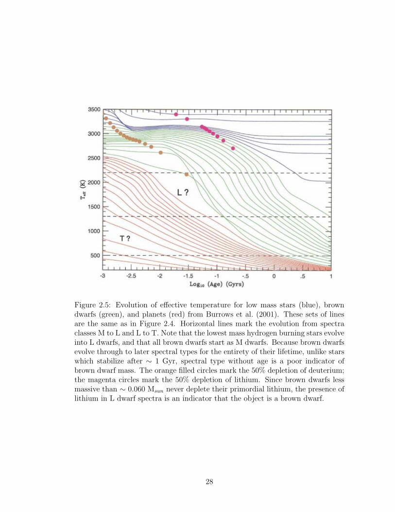
Figure 2.5: Evolution of effective temperature for low mass stars (blue), browndwarfs (green), and planets (red) from Burrows et al. (2001). These sets of linesare the same as in Figure 2.4. Horizontal lines mark the evolution from spectraclasses M to L and L to T. Note that the lowest mass hydrogen burning stars evolveinto L dwarfs, and that all brown dwarfs start as M dwarfs. Because brown dwarfsevolve through to later spectral types for the entirety of their lifetime, unlike starswhich stabilize after ∼ 1 Gyr, spectral type without age is a poor indicator ofbrown dwarf mass. The orange filled circles mark the 50% depletion of deuterium;the magenta circles mark the 50% depletion of lithium. Since brown dwarfs lessmassive than ∼ 0.060 Msun never deplete their primordial lithium, the presence oflithium in L dwarf spectra is an indicator that the object is a brown dwarf.
28

Effective Temperature of Low Mass Stars
1.00 0.10 0.01Mass (in Solar Mass)
0
2000
4000
6000
Effective T
em
pera
ture
(K
)
Max BD
Mass
T0 Dwarf
at ~1 Gyr
Deuterium
Limit
100 Myr
1 Gyr
5 Gyr
Figure 2.6: Effective Temperature as a function of mass for low mass stars andbrown dwarfs using the evolutionary models of Baraffe et al. (2003). Unlike stel-lar objects, the temperatures of brown dwarfs cool significantly with age; for anytemperature derived from photometry, nearly every brown dwarf mass may be pas-sible if age is not constrained. Conversely, while temperature changes rapidly early,brown dwarfs cool more slowly after several billion years, and precisely measuredmasses (∼10%) give little constraint to age. Low mass curves (M0 and later) usephotometry of Baraffe et al. (2003) and the spectral type-MJ relation of Cruz et al.(2003). High mass curves use the mass-luminosity relations of Henry & McCarthy(1993).
29
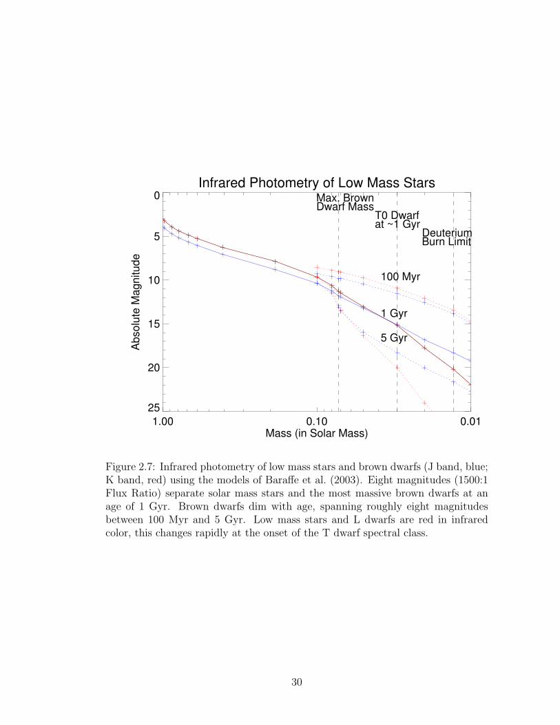
Infrared Photometry of Low Mass Stars
1.00 0.10 0.01Mass (in Solar Mass)
25
20
15
10
5
0
Absolu
te M
agnitude
Max. BrownDwarf Mass
T0 Dwarfat ~1 Gyr
DeuteriumBurn Limit
100 Myr
5 Gyr
1 Gyr
Figure 2.7: Infrared photometry of low mass stars and brown dwarfs (J band, blue;K band, red) using the models of Baraffe et al. (2003). Eight magnitudes (1500:1Flux Ratio) separate solar mass stars and the most massive brown dwarfs at anage of 1 Gyr. Brown dwarfs dim with age, spanning roughly eight magnitudesbetween 100 Myr and 5 Gyr. Low mass stars and L dwarfs are red in infraredcolor, this changes rapidly at the onset of the T dwarf spectral class.
30
the number of empirical constraints used to confirm and progress these models.
Model-independent measurements of brown dwarf masses provide the strongest
constraints on evolution models; i.e., ”mass benchmarks” to which evolution pre-
dictions can be compared Liu et al. (2008). Fundamental properties such as ef-
fective temperature are about five times better constrained with dynamical mass
measurements than with measurements of age.
Directly imaging a brown dwarf companion to another star and tracking its or-
bit provides the most readily available method for model-independent mass mea-
surements. With relative astrometry provided by direct imaging, one is able to
directly measure the total mass of the system. When combined with radial veloc-
ity, one obtains the masses of the individual components.
Companion detections through radial velocity alone give access to only to the
quantity M sin i, a combination of the companion mass and its orbital inclination,
and requires direct imaging of the pair to break this degeneracy. Detections by
transit give access to both the mass and radius of the brown dwarf (assuming the
mass and radius of the host star can be accurately determined by stellar models),
but are rare: only one brown dwarf is so far known by transit (Stassun et al.,
2006).
Binary measurements give three constraints on the suite of models: mass; pho-
tometry, which can be used to obtain total luminosity from empirical relations; and
the assumption that both objects are the same age, even if that age is unknown
(co-evolution). As mentioned in the previous subsection, these three constraints
allows one to calculate the system age using evolution models. For a given system
age, one can directly calculate the mass and photometry (or luminosity) of each
31
component until the optimal age is found (Liu et al., 2008)
Likewise, effective temperature can be derived for the brown dwarfs because
evolution models also provide the radius (c.f. Equation 2.1). These quantities have
all been calculated using only evolution models and empirical relations.
Several approaches towards testing the evolution models can be used.
(1) On almost purely empirical bases, the evolution-derived effective tempera-
ture can be compared to temperatures for L and T dwarfs derived by Golimowski
et al. (2004), by using the relations of Knapp et al. (2004) to obtain the spectral
types of the binary components from their photometry. This comparison is rea-
sonably accurate and limited only by model-dependent radii used by Golimowski
et al. (2004), but these are predicted to vary by less than 30%.
(2) The atmospheric models can be used to fit photometric or spectral data to
obtain an alternative measure of effective temperature. In this circumstance, it is
not possible to discern whether the discrepancy arises from evolution or atmosphere
models, although atmosphere models are quite uncertain in their determination of
effective temperature (Liu et al., 2008).
(3) Measurements of the component masses can be compared directly to those
predicted by atmosphere and evolution models. Using Golimowski et al. (2004)
derived luminosities and atmospheric fits to photometry for effective temperature,
evolution models can be used to make an estimate of the masses and age of the
binary components. This approach is perhaps the most natural comparison for
the purposes outlined in the introduction and has been used by Konopacky et al.
(2010).
32
To date, mass measurements of ”meaningful” precision (. 30%) have been
made of only nine systems which contain brown dwarfs; several other systems have
been measured with much less precision (& 60%) (Konopacky et al., 2010; Dupuy
et al., 2011). All but one of these brown dwarfs are M or L dwarfs.
Still, even this small subset shows systematic discrepancies when compared to
models. Konopacky et al. (2010) and Liu et al. (2008) both show that temperatures
derived with atmosphere models are generally inconsistent with those derived from
evolutionary models. In particular, atmosphere models predict temperatures lower
than evolution models by about 200-300 K for L dwarfs, although this systematic
trend appears to reverse for the single T dwarf with measured masses. Alterna-
tively, if atmosphere and evolution models are used to predict the brown dwarf
masses from photometry, this method incorrectly yields masses too low by 50-70%
for L dwarfs (and too high for the T dwarf).
Thus, one must exhibit caution when using these models to predict the masses
of substellar objects. In particular, this indicates that imaged exoplanets, such as
the planetary companions to HR 8799 (masses of 7, 10, and 10 MJ), are likely to
also be systematically in error (Marois et al., 2008).
One must recognize that a large subset of much more precisely measured masses
spanning the entire range of brown dwarf masses are necessary to begin challenging
evolution models. This is particularly evident when one keeps in mind that inherent
in the atmospheric models are assumptions of opacities, metallicities, cloud models,
etc., all of which operate in tandem with evolution models to predict the mass or
age of a binary system. Radius, for instance, may span a wide range (perhaps
25%) for a given mass and age for hot, evolving brown dwarfs depending on cloud
formation and elemental composition (Burrows et al., 2011). To truly carve into
33
our understanding of brown dwarfs requires many additional benchmarks against
which these models can be tested.
2.4 The Challenge of Resolving Brown Dwarf Binaries
A confluence of natural and technical challenges has prevented the brown dwarf
community from amassing a larger database of precisely measured brown dwarf
masses. Resolving brown dwarfs as companions to stellar and sub-stellar objects
and the subsequent tracking of their orbits requires overcoming several challenges.
Four criteria must be satisfied to detect brown dwarf companions and acquire
measurements of their dynamical masses:
1. The orbital period must be short enough to track the nearly full or full orbit
in a reasonable length of time; this, equivalently, requires binaries with small
primary-secondary separations.
2. Technology and/or techniques can be obtained that can achieve high enough
levels of angular resolution to resolve the individual components of the binary,
given the distortions introduced by the atmosphere.
3. Given the level of image contrast that technique is able to achieve (usually
as a function of separation), the faint brown dwarf can be identified above
photon noise, background noise, detector noise, or more usually, the glare of
the primary star and/or systematic errors which distort image quality.
4. That such a potential system exist at a location in the sky which allows the
above three constraints to be satisfied.
34
In other words, given the technical challenges at telescopes and the natural
distribution of stars, what brown dwarf systems can we observe?
2.4.1 Angular Resolution for Brown Dwarf Dynamical
Masses
To obtain precisely measured brown dwarf masses, one necessitates high-contrast
and high-angular resolution capabilities.
The period, T , of a binary scales with Kepler’s Third Law:
T 2 = (2π)2a3/GMtotal(T
1 yr
)2
=( a
1 AU
)3(
1 M�Mtotal
)(2.2)
where a is the semi-major axis of the orbit and Mtotal is the combined mass of the
binary. Obtaining dynamical mass requires tracking a full or nearly full orbit; to
track the orbit in reasonable amount of time (a few years) requires resolving very
closely-separated (. a few AU) binaries.
This is shown quantitatively in Figure 2.8. The figure shows the period of a
0.070 M� brown dwarf in orbit around primaries of various spectral types and a
range of semi-major axes. Orbital period clearly rises quickly with semi-major
axis; to find a binary with periods shorter than 5 years requires the detection of
brown dwarf companions at separations closer than about 3 AU.
Nearby field stars in the solar neighborhood span distances of & 10-100 parsecs.
For binary systems at a given distance, the semi-major axis corresponds to an
35
angular separation of:
θbd = 100 mas×( a
1 AU
)(dsystem10 pc
). (2.3)
From this we conclude that dynamical mass measurements require a capability to
resolve brown dwarf companions at separations closer than 300 mas (∼ 5.× 10−4
degrees).
2.4.2 Primary-Secondary Contrasts for Brown Dwarf
Companions
Late-Type Primaries are Favorable
Despite the ’flux enhancement’ in the infrared of brown dwarfs due to their opacity
sources, the contrast between a solar type star and the most massive brown dwarfs
at an age of 1 billion years is roughly eight magnitudes (1500:1 flux ratio). This
contrast drops to six magnitude (200:1 flux ratio) when the primary is an M0 dwarf
(Figures 2.7 and 2.9). Assuming that equal imaging performance can be achieved
for both primaries, there is a large benefit to surveying late-type stars (M and K
dwarfs).
Youthful Systems are Favorable
Unlike stars, which retain their brightness throughout their lives, brown dwarfs
dim by a factor of ∼10 while aging from 100 million to 1 billion years, and another
factor of∼10 by 5 billion years. Indeed, this signals another strategy for companion
searches: young systems. These systems also yield insight into the early stages
36
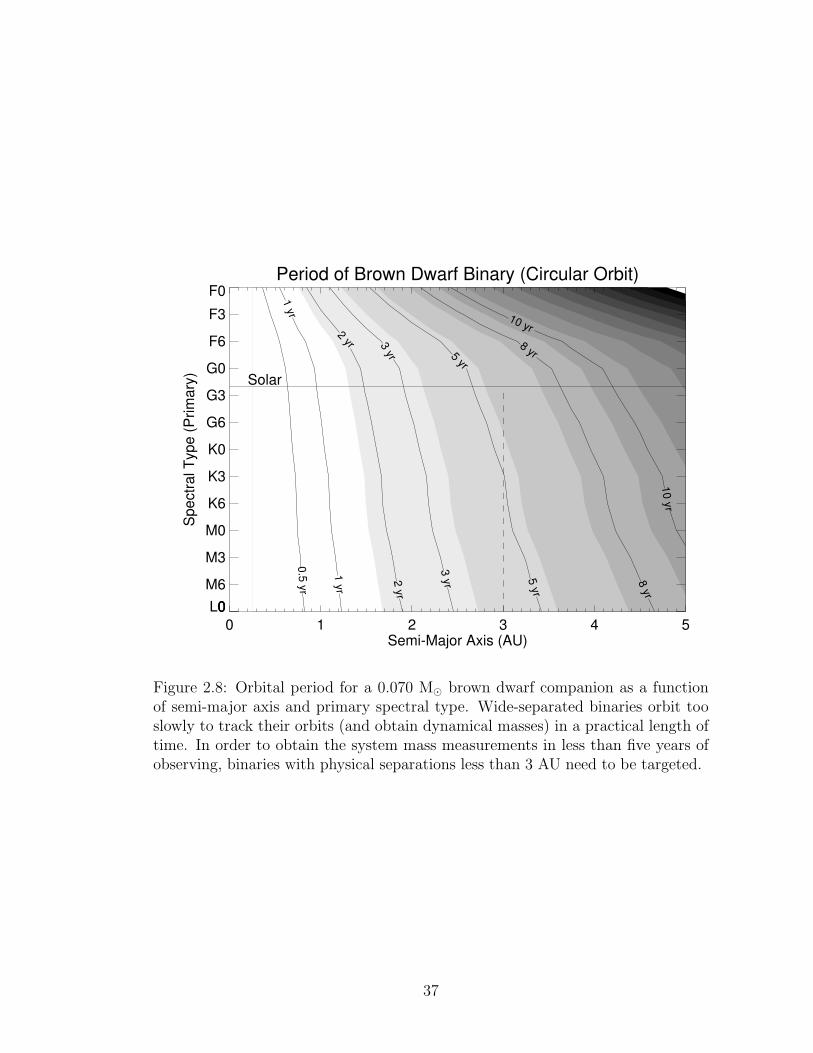
Period of Brown Dwarf Binary (Circular Orbit)
0 1 2 3 4 5Semi-Major Axis (AU)
L0
M6
M3
M0
K6
K3
K0
G6
G3
G0
F6
F3
F0
00
Sp
ectr
al T
yp
e (
Prim
ary
)
0.5
yr
1 y
r
1 yr
2 y
r
2 yr
3 y
r
3 yr
5 yr
5 yr
8 yr
8 yr
10 y
r
10 yr
Solar
Figure 2.8: Orbital period for a 0.070 M� brown dwarf companion as a functionof semi-major axis and primary spectral type. Wide-separated binaries orbit tooslowly to track their orbits (and obtain dynamical masses) in a practical length oftime. In order to obtain the system mass measurements in less than five years ofobserving, binaries with physical separations less than 3 AU need to be targeted.
37
of brown dwarf evolution and formation by exploring, for instance, the structure
evolution of young brown dwarfs or their migration mechanism (Kraus et al., 2008,
2009).
Unfortunately, age is a difficult parameter to measure for individual stars and
the distribution of stellar ages in the solar neighborhood is roughly flat. Corre-
lations between age and activity have been successfully used to identify clusters
of similarly youthful stars in the solar neighborhood. Several of these young as-
sociations and moving groups have been identified in the northern hemisphere
(Zuckerman, 2004; Torres et al., 2006). To date, the youngest clusters are rela-
tively far away (e.g., Upper Sco: roughly 5 million years and 140 parsecs). At
such great distances, even higher resolution is needed for dynamical masses (e.g.,
diffraction limited H band observations correspond to physical separations of 1.1
AU at 140 parsecs). Alternatively, clusters of nearby, moderate age collections
offer a potent compromise between youth and proximity (ages 10-150 million years
at distances of 10-50 parsecs), while also providing insights into the evolution of
brown dwarf systems with age. Several moving groups are known in the northern
hemisphere and many more in the southern hemisphere. Moving group identifi-
cation is an observationally intensive project and cataloging the late-type (M and
K dwarf) members of these groups has only recently begun (Schlieder & Lepine,
2010). Both of these surveys will provide fertile grounds for upcoming brown dwarf
and exoplanet imaging surveys and for the studies of young brown dwarfs.
Mid-Infrared Bands are Favorable
Finally, one can consider the advantages of observing at the longer wavelengths of
the mid-infrared (2-10µm). Like the near infrared, brown dwarfs are flux enhanced
38
at mid-infrared wavelengths and the nominal blackbody contrasts are also more
favorable at longer wavelengths. The impact of atmospheric turbulence is greatly
reduced at longer wavelengths, in fact, 5-meter class telescopes are nearly diffrac-
tion limited at 10µm, and turbulence evolves more slowly, allowing for slower run
wavefront sensors and fainter natural guide stars. While direct imaging in the
mid-infrared will certainly play a role in future exoplanet surveys, adaptive optics
technologies have just recently begun to come online at these wavelengths (e.g.,
MMT Telescope, Wildi et al. (2003)).
2.4.3 Adaptive Optics: Resolution
Measuring the mass of brown dwarfs by orbit tracking in a few years requires
resolution reaching approximately 300 mas or better. Resolving brown dwarfs
requires contrasts of 102-103:1 in order to detect brown dwarf companions to solar
type stars in the infrared. A far easier aim is to resolve companions in orbit around
brown dwarf primaries. In this section, we explore the technical feasibility of these
observations using current technology in the infrared.
An optically perfect telescope, observing a point source through a still and
homogeneous atmosphere will image a spot of angular size 1.22 λ/D, where D is
the diameter of the telescope aperture and λ is the wavefront of the observation.
As a point of reference, the 200” Hale Telescope at Palomar Observatory (5.08 m)
observing in the infrared H band (1.6 µm) images a spot size ∼65 milliarcseconds
in radius.
Distinguishing two closely separated objects is the primary challenges of direct
imaging for high angular resolution. The finite size of a point source provides
39
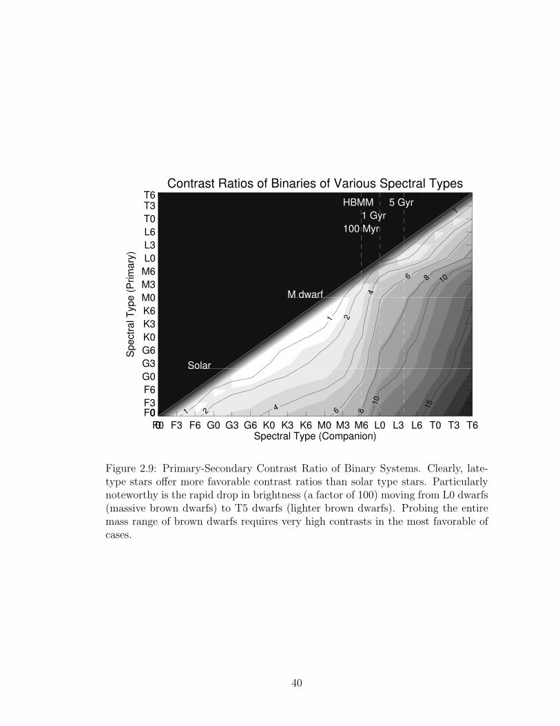
Contrast Ratios of Binaries of Various Spectral Types
F0 F3 F6 G0 G3 G6 K0 K3 K6 M0 M3 M6 L0 L3 L6 T0 T3 T600Spectral Type (Companion)
F0F3
F6
G0
G3
G6
K0
K3
K6
M0
M3
M6
L0
L3
L6
T0
T3T6
00
Sp
ectr
al T
yp
e (
Prim
ary
)
1
1
1
2
2
4
4
6
6
8
8
10
10
15
M dwarf
Solar
100 Myr
1 Gyr
5 GyrHBMM
Figure 2.9: Primary-Secondary Contrast Ratio of Binary Systems. Clearly, late-type stars offer more favorable contrast ratios than solar type stars. Particularlynoteworthy is the rapid drop in brightness (a factor of 100) moving from L0 dwarfs(massive brown dwarfs) to T5 dwarfs (lighter brown dwarfs). Probing the entiremass range of brown dwarfs requires very high contrasts in the most favorable ofcases.
40
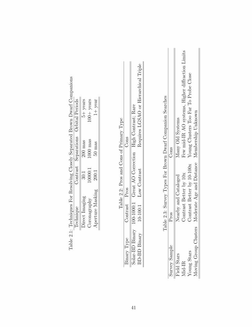
Tab
le2.
1:T
echniq
ues
For
Res
olvin
gC
lose
lySep
arat
edB
row
nD
war
fC
ompan
ions
Tec
hniq
ue
Con
tras
tSep
arat
ions
Orb
ital
Per
iods
Dir
ect
Imag
ing
30:1
200
mas
5+ye
ars
Cor
onag
raphy
1000
0:1
1000
mas
100+
year
sA
per
ture
Mas
kin
g20
0:1
50m
as1+
year
Tab
le2.
2:P
ros
and
Con
sof
Pri
mar
yT
yp
eB
inar
yT
yp
eC
ontr
ast
Pro
sC
ons
Sol
ar-B
DB
inar
y10
0-10
00:1
Gre
atA
OC
orre
ctio
nH
igh
Con
tras
t;R
are
BD
-BD
Bin
ary
10-1
00:1
Low
Con
tras
tR
equir
esL
GSA
Oor
Hie
rarc
hic
alT
riple
Tab
le2.
3:Surv
eyT
yp
esF
orB
row
nD
war
fC
ompan
ion
Sea
rches
Surv
eySam
ple
Pro
sC
ons
Fie
ldSta
rsN
earb
yan
dC
atal
oged
Man
yO
ldSyst
ems
Mid
-IR
Con
tras
tB
ette
rby
10x
Few
mid
-IR
AO
syst
ems,
Hig
her
diff
ract
ion
Lim
its
You
ng
Sta
rsC
ontr
ast
Bet
ter
by
10-1
00x
You
ng
Clu
ster
sT
oo
Far
To
Pro
be
Clo
seM
ovin
gG
roup
Clu
ster
sM
oder
ate
Age
and
Dis
tance
Mem
ber
ship
Unknow
n
41
an estimate for the smallest angle by which separate objects can be resolved, the
so-called diffraction limited resolution:
θmin =1.22λ
D. (2.4)
The criterion is only a rule-of-thumb; one can certainly imagine an experiment
taking images so precisely that the overlap of two such spots could be distinguished
by, for instance, the elongation of the spot in one direction.
However, the atmosphere is a turbulent, inhomogeneous window through which
the stars are observed. Variations in the temperature and index of refraction
deform the phase and amplitude of the incoming wavefront. These spatial and
temporal variations of the wavefront distort the image and degrade image quality.
Typically, these seeing effects blur out point sources in long exposures and prevent
one from reaching angular resolution finer than about one arcsecond (1000 mas).
To minimize the effects of atmospheric turbulence, major efforts within the
field aim to develop real-time optical components able to measure and counteract
wavefront errors; these systems are generally referred to as adaptive optics or AO. A
typical system consists of a feedback loop a system for measure real-time wavefront
shape across the telescope pupil at a speed of about a thousand measurements
per second and system between a deformable mirror without about a thousand
actuators. Good adaptive optics systems can remove so much of the atmospheric
turbulence that the resulting image approaches that of the diffraction limit. With
deconvolution algorithms, one is often able to obtain diffraction limited resolution;
although ones chances of seeing a particularly faint companion at these separations
is not particularly high.
A diffraction-limited adaptive optics-corrected infrared image is shown in Fig-
ure 2.10. The image is a typical long exposure H band (1.6µm) image taken by
42
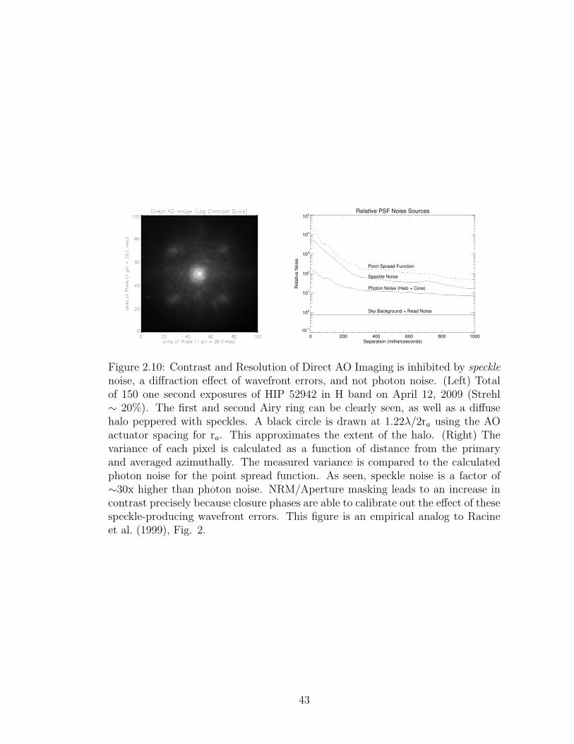
Relative PSF Noise Sources
0 200 400 600 800 1000Separation (milliarcseconds)
10-1
100
101
102
103
104
105
Re
lative
No
ise
Point Spread Function
Speckle Noise
Photon Noise (Halo + Core)
Sky Background + Read Noise
Figure 2.10: Contrast and Resolution of Direct AO Imaging is inhibited by specklenoise, a diffraction effect of wavefront errors, and not photon noise. (Left) Totalof 150 one second exposures of HIP 52942 in H band on April 12, 2009 (Strehl∼ 20%). The first and second Airy ring can be clearly seen, as well as a diffusehalo peppered with speckles. A black circle is drawn at 1.22λ/2ra using the AOactuator spacing for ra. This approximates the extent of the halo. (Right) Thevariance of each pixel is calculated as a function of distance from the primaryand averaged azimuthally. The measured variance is compared to the calculatedphoton noise for the point spread function. As seen, speckle noise is a factor of∼30x higher than photon noise. NRM/Aperture masking leads to an increase incontrast precisely because closure phases are able to calibrate out the effect of thesespeckle-producing wavefront errors. This figure is an empirical analog to Racineet al. (1999), Fig. 2.
43
the PHARO infrared imaging instrument (Hayward et al., 2001) on the 200” Hale
Telescope. The complex structure of an adaptively corrected image is immediately
apparent:
1. Diffraction Core: At this level of correction, the bright diffraction core is
evident at the center of the image, surrounded by the first two Airy rings.
The strong presence of the diffraction core allows the extraction of diffrac-
tion limited resolution. The central location of the first two Airy rings are
1.64λ/D and 2.78λ/D, respectively.
2. Halo: A diffuse halo of flux encircles the diffraction core. This light is dis-
placed from the core by the effect of small-scale inhomogeneities of the wave-
front, perturbations which are on scales smaller than the adaptive optics
actuator size and can’t be measured or corrected. The surface intensity (the
flux level) of this halo depends critically on the level of correction. However,
if adaptive optics correction is consistent, deconvolution algorithms can re-
move some of the halo. The faintest object that can be detected within this
halo depends on the success of these measures.
3. AO Control Radius: The finite spacing of the adaptive optics actuators pre-
vents correction of the small-scale wavefront errors which develop the image
far away from the diffraction core. The extent to which the AO system can
impact image quality is about 1.22λ/2ra; this is the approximate extend
of the halo. Beyond this region, the image quality is no different than an
uncorrected image.
4. Speckles: Near the first Airy ring and within the halo, one can observe a fine
granular structure to the flux distribution. These grains are speckles, formed
by large-scale wavefront errors not corrected by the adaptive optics system.
44
The last decade of high contrast imaging has shown that speckles set the
ultimate limits for the contrast one can achieve with an imaging system.
The typical metric for measuring the quality of AO correction is the Strehl
ratio, S, the ratio of the peak flux of the corrected point spread function to the
ideal diffraction limited point spread function. Good correction in the infrared for
current systems can achieve Strehl ratios of 10-30%. The percentage of the total
flux contained within the diffraction core is also ∼ S; the percentage of flux within
the halo is ∼ 1− S.
The level of correction is a sensitive function of the observing wavelength and
brightness of the target. Shorter wavelengths experience more wavefront error
and variance on shorter timescales, and are thusly more challenging to correct.
Most importantly, the target must be bright enough to adequately illuminate the
wavefront sensor (in the waveband in it uses to sense). The wavelength and the
quality and timescale of atmospheric seeing set roughly the rate at which the AO
system must run to effectively reduce the effects of turbulence.
The adaptive optics wavefront sensor requires a sufficiently bright ’guide’ star
to provide a reference; this can be the science target itself or a nearby object
(usually less than 1 arcminute). The Palomar AO system achieves diffraction
limited observing in the infrared (Strehl ∼50% in Ks) using guide stars brighter
than V∼10 in typical seeing, with functionality down to V∼12. The celestial
distribution of stars bright enough to drive adaptive optics covers less than about
1% of the total sky area. The brightness limit of adaptive optics system eliminates
the prospect of observing confirmed, isolated brown dwarfs and other visually faint
targets with adaptive optics.
45
Figure 2.11 shows the absolute visual magnitude of solar-mass and low mass
stars. Given the technical requirements of natural guide star adaptive optics, we
conclude that companion searches for brown dwarfs aiming to make mass measure-
ments must survey nearby stars of type earlier than about M3. As a rule-of-thumb,
the resolution of brown dwarf companions to M3 dwarfs requires infrared contrasts
of at least 100:1 or higher at separations closer than 300 mas.
One exception which enables the exploration of even lower mass primaries for
companions is the case in which this binary orbits another star which acts as a
natural guide stars, i.e., a hierarchical triple system. This has allowed detailed
study of two nearby brown dwarf-brown dwarf binaries using the triplet primaries
as natural guide stars: GJ 802b (Pravdo et al., 2005; Lloyd et al., 2006; Ireland
et al., 2008) and GJ 569B (Lane et al., 2001; Osorio et al., 2004).
Laser Guide Star Adaptive Optics
Another exception for exploring very low mass stars for companions with high
resolution relies on the continued development of new Laser Guide Star Adaptive
Optics systems (Palomar, Roberts et al. (2008); Keck, Wizinowich (2006)). These
systems use a 589nm sodium laser to excite a patch of the sodium layer in the
upper atmosphere. This excited path acts as the guide star to drive high order
wavefront correction. This system still requires a bright star close to the science
target for low order corrections, but with greatly relaxed constraints (as much as
60 arcminutes without loss of correction, down to visible magnitudes of 17.5).
Laser guide star adaptive optics systems allow diffraction limited imaging of
faint targets, including companion searches using brown dwarfs as primaries. This
greatly alleviates the difficulties of contrast ratios and enables mass measurements
46
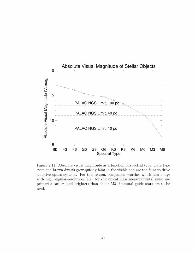
Absolute Visual Magnitude of Stellar Objects
F0 F3 F6 G0 G3 G6 K0 K3 K6 M0 M3 M600Spectral Type
15
10
5
0
Absolu
te V
isual M
agnitude (
V, m
ag)
PALAO NGS Limit, 10 pc
PALAO NGS Limit, 40 pc
PALAO NGS Limit, 100 pc
Figure 2.11: Absolute visual magnitude as a function of spectral type. Late typestars and brown dwarfs grow quickly faint in the visible and are too faint to driveadaptive optics systems. For this reason, companion searches which aim imagewith high angular-resolution (e.g. for dynamical mass measurements) must useprimaries earlier (and brighter) than about M3 if natural guide stars are to beused.
47
of systems ensured to contain brown dwarfs.
The LGSAO system on Keck has been a boon for dynamical mass measurements
of brown dwarfs. In fact, all but three of the dynamically measured brown dwarf
masses have come from LGSAO programs (Konopacky et al., 2010; Dupuy et al.,
2010): the two previously mentioned brown dwarf hierarchical systems and one
system detected in transit (Stassun et al., 2006).
2.4.4 Adaptive Optics: Contrast
The faintest companion one can detect (the image contrast) is most basically a
simpler question: How faint can a companion source be before the observer can no
longer distinguish the flux of the companion source from noise sources?
The obtainable contrast one achieves is a function of separation from the
primary. As discussed in the previous section, close to the primary and within
the halo, residual wavefront phase errors uncorrected by the AO system produce
diffraction effects which litter the image with bright speckles. Speckles are not
placed randomly throughout the halo, but are preferentially pinned to the first
and second Airy rings (Bloemhof et al., 2000, 2001; Sivaramakrishnan et al., 2003).
The precise location of the speckles shift on timescales of tens of seconds to tens of
minutes (Figure 2.12). Speckles pinned to the first Airy ring introduced variations
of as much as 10% the peak flux over ten minutes (2-5% on the second Airy ring)
and changed locations irregularly. Because of the slowly varying nature of these
speckles, they are referred to as quasi-static speckles.
As mentioned in the Perspective of this manuscript, the impact of wavefront
errors arising from imperfect optics have been extensively explored in recent years,
48
mostly in the pursuit of high-contrast coronagraph observations (Lafreniere et al.,
2007). Optical components of the telescope located after the wavefront sensor
cannot be corrected by adaptive optics and produce non-common path wavefront
errors. These wavefront errors evolve due to temperature or pressure changes,
mechanical flexures, guiding errors, changing illumination of the primary mirror,
or other phenomena (Marois et al., 2005, 2006).
Quasi-static speckles dominate long exposures within separations of 5-10 arc-
seconds at the Keck and Palomar Hale Telescopes. They evolve too slowly to
effectively average out over even hour long exposures (Hinkley et al., 2007; Macin-
tosh et al., 2005; Metchev et al., 2003). With no mechanism to distinguish speckles
from true companions, longer exposures will not yield any higher contrasts; it is
not the stochastic variation of quasi-static speckles which cause them to hinder
high contrast imaging. Thus, contrast limits are not set by the variation of the
quasi-static speckles over a set of images, but by their mean brightness. Unequiv-
ocally, quasi-static speckles set the ultimate noise floor of high contrast imaging,
generating a slowly varying distribution of flux that can be mistaken for faint com-
panions.
Figure 2.13 shows typical 3-sigma contrast limits one can reach with direct
imaging in H band using the Palomar AO system and PHARO camera. As evident,
high contrast imaging is quite limited at close separations, and significantly less
than what would be required to resolve brown dwarfs in orbit around even the
lowest mass stars (100:1 or better).
Non-Redunant Aperture Masking Interferometry, through its use of closure
phases, enables higher detection contrasts at close separations because closure
phases are not affected by the wavefront errors which produce quasi-static speck-
49
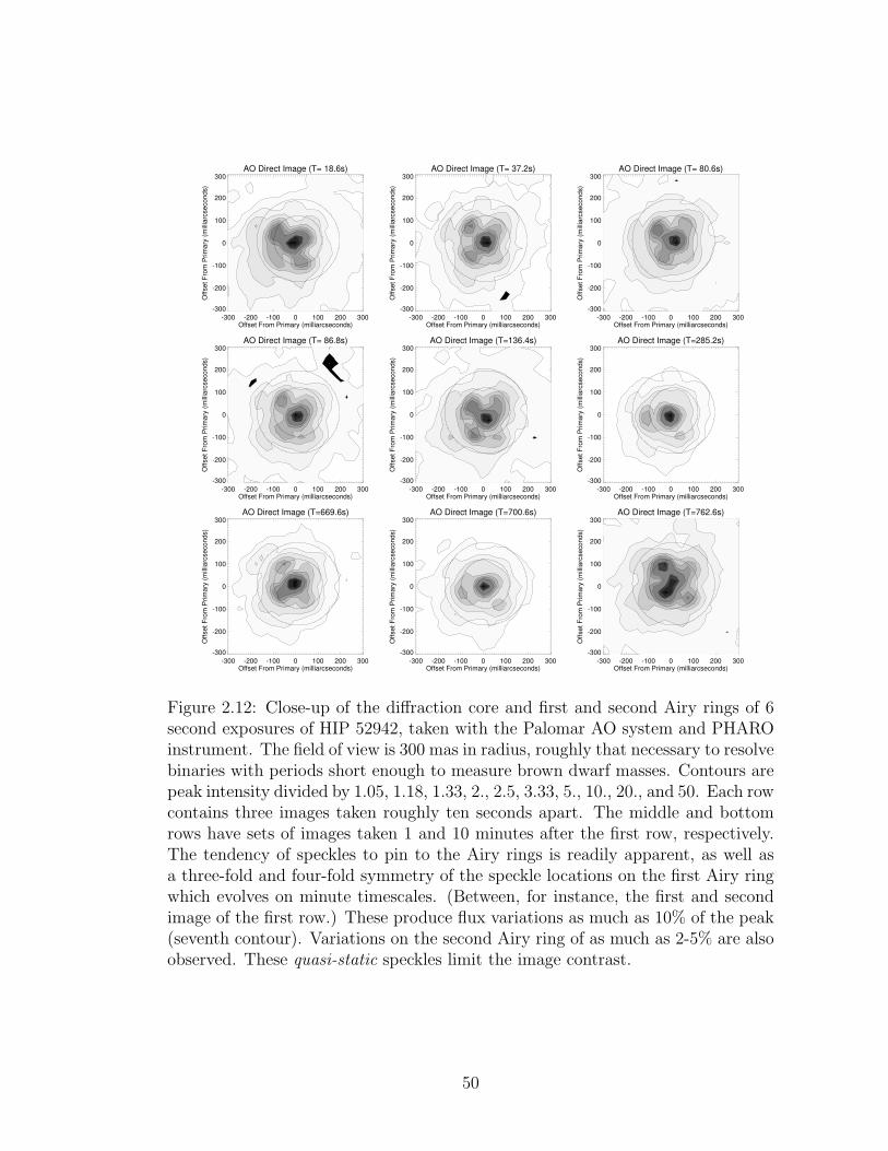
AO Direct Image (T= 18.6s)
-300 -200 -100 0 100 200 300Offset From Primary (milliarcseconds)
-300
-200
-100
0
100
200
300
Off
se
t F
rom
Prim
ary
(m
illia
rcse
co
nd
s)
AO Direct Image (T= 37.2s)
-300 -200 -100 0 100 200 300Offset From Primary (milliarcseconds)
-300
-200
-100
0
100
200
300
Off
se
t F
rom
Prim
ary
(m
illia
rcse
co
nd
s)
AO Direct Image (T= 80.6s)
-300 -200 -100 0 100 200 300Offset From Primary (milliarcseconds)
-300
-200
-100
0
100
200
300
Off
se
t F
rom
Prim
ary
(m
illia
rcse
co
nd
s)
AO Direct Image (T= 86.8s)
-300 -200 -100 0 100 200 300Offset From Primary (milliarcseconds)
-300
-200
-100
0
100
200
300
Off
se
t F
rom
Prim
ary
(m
illia
rcse
co
nd
s)
AO Direct Image (T=136.4s)
-300 -200 -100 0 100 200 300Offset From Primary (milliarcseconds)
-300
-200
-100
0
100
200
300
Off
se
t F
rom
Prim
ary
(m
illia
rcse
co
nd
s)
AO Direct Image (T=285.2s)
-300 -200 -100 0 100 200 300Offset From Primary (milliarcseconds)
-300
-200
-100
0
100
200
300
Off
se
t F
rom
Prim
ary
(m
illia
rcse
co
nd
s)
AO Direct Image (T=669.6s)
-300 -200 -100 0 100 200 300Offset From Primary (milliarcseconds)
-300
-200
-100
0
100
200
300
Off
se
t F
rom
Prim
ary
(m
illia
rcse
co
nd
s)
AO Direct Image (T=700.6s)
-300 -200 -100 0 100 200 300Offset From Primary (milliarcseconds)
-300
-200
-100
0
100
200
300
Off
se
t F
rom
Prim
ary
(m
illia
rcse
co
nd
s)
AO Direct Image (T=762.6s)
-300 -200 -100 0 100 200 300Offset From Primary (milliarcseconds)
-300
-200
-100
0
100
200
300
Off
se
t F
rom
Prim
ary
(m
illia
rcse
co
nd
s)
Figure 2.12: Close-up of the diffraction core and first and second Airy rings of 6second exposures of HIP 52942, taken with the Palomar AO system and PHAROinstrument. The field of view is 300 mas in radius, roughly that necessary to resolvebinaries with periods short enough to measure brown dwarf masses. Contours arepeak intensity divided by 1.05, 1.18, 1.33, 2., 2.5, 3.33, 5., 10., 20., and 50. Each rowcontains three images taken roughly ten seconds apart. The middle and bottomrows have sets of images taken 1 and 10 minutes after the first row, respectively.The tendency of speckles to pin to the Airy rings is readily apparent, as well asa three-fold and four-fold symmetry of the speckle locations on the first Airy ringwhich evolves on minute timescales. (Between, for instance, the first and secondimage of the first row.) These produce flux variations as much as 10% of the peak(seventh contour). Variations on the second Airy ring of as much as 2-5% are alsoobserved. These quasi-static speckles limit the image contrast.
50
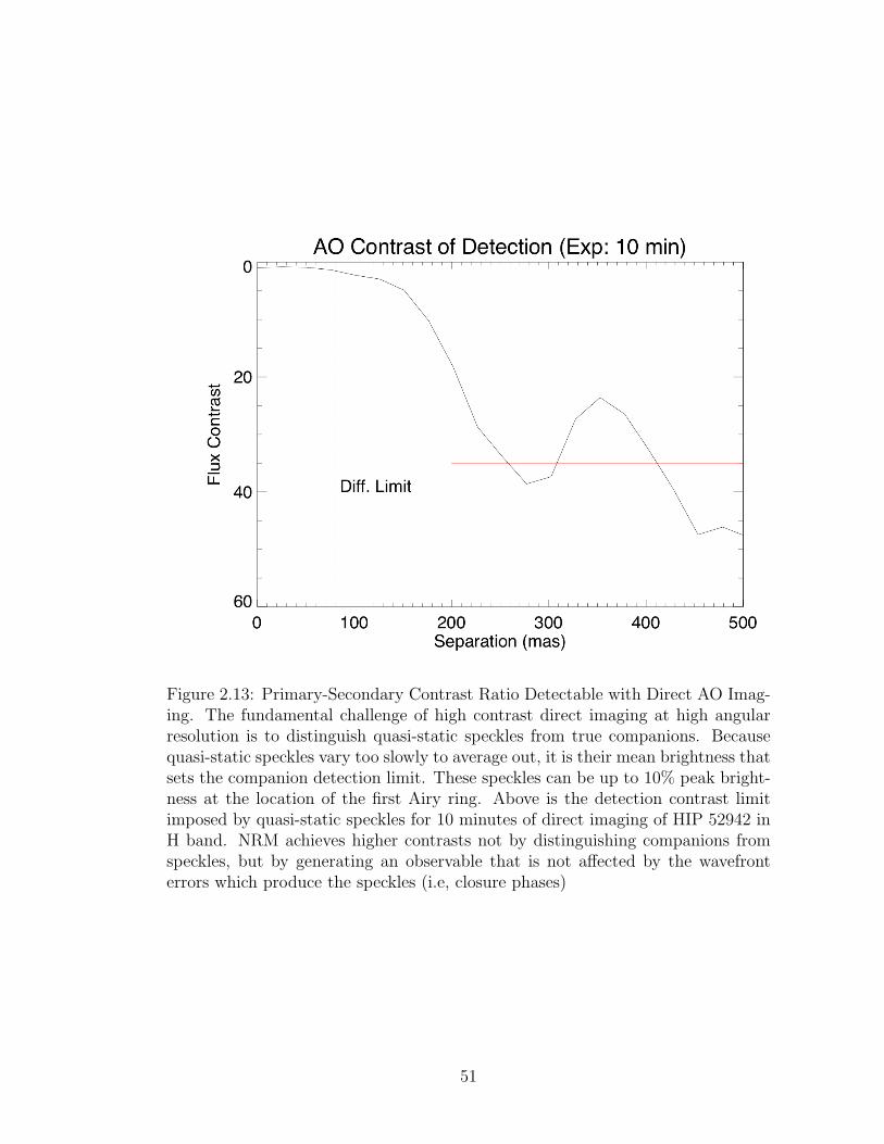
Figure 2.13: Primary-Secondary Contrast Ratio Detectable with Direct AO Imag-ing. The fundamental challenge of high contrast direct imaging at high angularresolution is to distinguish quasi-static speckles from true companions. Becausequasi-static speckles vary too slowly to average out, it is their mean brightness thatsets the companion detection limit. These speckles can be up to 10% peak bright-ness at the location of the first Airy ring. Above is the detection contrast limitimposed by quasi-static speckles for 10 minutes of direct imaging of HIP 52942 inH band. NRM achieves higher contrasts not by distinguishing companions fromspeckles, but by generating an observable that is not affected by the wavefronterrors which produce the speckles (i.e, closure phases)
51
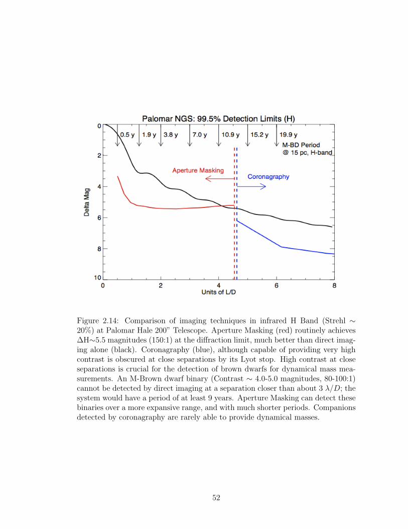
Figure 2.14: Comparison of imaging techniques in infrared H Band (Strehl ∼20%) at Palomar Hale 200” Telescope. Aperture Masking (red) routinely achieves∆H∼5.5 magnitudes (150:1) at the diffraction limit, much better than direct imag-ing alone (black). Coronagraphy (blue), although capable of providing very highcontrast is obscured at close separations by its Lyot stop. High contrast at closeseparations is crucial for the detection of brown dwarfs for dynamical mass mea-surements. An M-Brown dwarf binary (Contrast ∼ 4.0-5.0 magnitudes, 80-100:1)cannot be detected by direct imaging at a separation closer than about 3 λ/D; thesystem would have a period of at least 9 years. Aperture Masking can detect thesebinaries over a more expansive range, and with much shorter periods. Companionsdetected by coronagraphy are rarely able to provide dynamical masses.
52

les. NRM when combined with AO does not remove quasi-static speckles, per se.
Instead, NRM closure phases are a dataset that are invariant to many pupil-plane
phase errors. In effect, closure phases can mitigate the quasi-static problem in a
single image.
Aperture masking with adaptive optics is well-established for resolving stellar
companions at and within the formal diffraction limit (down to 0.5λ/D) and at
high contrasts (200:1 at λ/D)(Tuthill et al., 2000; Lloyd et al., 2006; Ireland et al.,
2008; Martinache et al., 2007). This range of high-resolution and high-contrast
make aperture ideal for close companion searches and dynamical mass measure-
ments (Figure 2.14). Companions detected with aperture masking also have a
similarly higher precision photometry and astrometry, providing much higher pre-
cision dynamical masses up to an order of magnitude higher.
The use of NRM with adaptive optics enables the detection of brown dwarf
companions to K and M dwarfs for Strehls of 30% for typical field stars (i.e., ages
of a few billion years). This level of adaptive optics correction is routinely achieved
by most natural guide star adaptive optics systems.
When combined with laser guide star adaptive optics system (e.g., Keck, Wiz-
inowich (2006)) at similar performance levels, NRM offers a method for measuring
brown dwarf masses to much higher precision (less than 10%) than those currently
available in the literature. If NRM with LGSAO is able to reach 200:1 contrasts
using brown dwarf primaries, the technique may potentially be able to resolve
companions through the entire mass range of brown dwarfs. This could provide
much needed mass measurements of cool brown dwarfs and even young, massive
exoplanets.
53
The development of a laser guide star adaptive optics program at Palomar
(Roberts et al., 2008) motivated my high-angular resolution companion search to
nearby brown dwarfs using NRM: Bernat et al. (2010), c.f. Chapter 5: A Close
Companion Search Around L Dwarfs Using Aperture Masking Interferometry and
Palomar Laser Guide Star Adaptive Optics.
54
CHAPTER 3
NON-REDUNDANT APERTURE MASKING INTERFEROMETRY
WITH ADAPTIVE OPTICS
A substantial literature exists to detail the long heritage of seeing-limited aper-
ture masking (?Baldwin et al., 1986; Haniff et al., 1987; Roddier, 1986; Readhead
et al., 1988; Cornwell, 1989; Tuthill et al., 2000), which itself draws on speckle
interferometry (?). Noll (1976) showed that 87% of the spectral power of atmo-
spheric (Kolmogorov) turbulence produces tip and tilt wavefront errors which only
serve to move the image around the detector but not degrade its structure. Over
long exposures (i.e., over several iterations of the atmosphere, roughly tens of mil-
liseconds in the infrared), this movement smears the image, producing the blurry
seeing-limited point spread function. Exposures short enough that the atmosphere
can be treated as static offer an opportunity to retrieve images which are essentially
unaffected by 7/8th of the atmospheric wavefront errors.
Positioning a non-redundant aperture mask in the pupil plane of the telescope
or instrument transforms the full aperture into a sparsely populated set of sub-
apertures (Figure 3.1). Provided the telescope instrument gives access to the pupil
plane, such as the location of the Lyot stop within a coronagraph, then this is
a convenient location to place the mask. Alternatively, the mask can be placed
directly on the primary or secondary mirrors (e.g., Tuthill et al. (2000)). The
resulting image produced is a set of over-lapping fringes called the interferogram.
The amplitude and phase of each fringe corresponds to the measurement of one
particular component of the target complex visibility, i.e., the Fourier Transform
of the target brightness distribution. Multiplying the complex visibility of specific
baseline triplets creates bispectra (Lohmann et al., 1983), the argument of which
55
is the closure phase (Jennison, 1958; Cornwell, 1989). Closure phases are robust
against many forms of pupil-plane phase errors, and enables diffraction-limited
imaging in seeing-limited conditions, provided that exposures are short. Closure
phase errors arise only from atmospheric phase errors on scales smaller than a sub-
aperture. In other words, closure phases rejects even more of the total spectral
power of atmospheric turbulence. In its relation to direct imaging, closure phases
are robust against precisely the wavefront phase errors that produce speckles close
to the core, resulting in much improved image contrast close to the core. Provided
that imaging is speckle or wavefront phase limited (Readhead et al., 1988; Racine
et al., 1999), aperture masking provides higher fidelity imaging than direct imaging
despite blocking a large percentage of the flux.
Adaptive optics systems, by design, aim to sharply reduce the spatial and
temporal variation of the wavefront. Current systems on 5-10 meter class telescopes
for infrared imaging provide stable and partially coherent wavefronts across the
entire sub-aperture. As discussed in the Chapter 1, current adaptive optics systems
can obtain near diffraction-limited resolution, but image contrast close to the core
(within a few λ/D) is hindered by quasi-static speckles arising from slowly varying
instrumental phase errors. When combined with AO, NRM provides increased
contrast at close separations (0.5-4.0λ/D) by reducing the impact of AO residual
phase errors (which produce the halo) and ultimately reaches deeper contrasts
(102-103:1) by mitigating the instrumental phase errors that produce quasi-static
speckles (Lloyd et al., 2006; Kraus et al., 2008; Hinkley et al., 2010).
This Chapter and Chapter 5 aim to provide a technical underpinning for NRM
with AO and to contribute to the growing body of investigation into limitations of
the technique and its improvement. Reviews of seeing-limited NRM are available
56
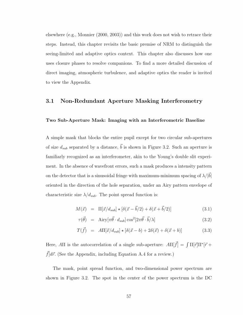
elsewhere (e.g., Monnier (2000, 2003)) and this work does not wish to retrace their
steps. Instead, this chapter revisits the basic premise of NRM to distinguish the
seeing-limited and adaptive optics context. This chapter also discusses how one
uses closure phases to resolve companions. To find a more detailed discussion of
direct imaging, atmospheric turbulence, and adaptive optics the reader is invited
to view the Appendix.
3.1 Non-Redundant Aperture Masking Interferometry
Two Sub-Aperture Mask: Imaging with an Interferometric Baseline
A simple mask that blocks the entire pupil except for two circular sub-apertures
of size dsub separated by a distance, ~b is shown in Figure 3.2. Such an aperture is
familiarly recognized as an interferometer, akin to the Young’s double slit experi-
ment. In the absence of wavefront errors, such a mask produces a intensity pattern
on the detector that is a sinusoidal fringe with maximum-minimum spacing of λ/|~b|
oriented in the direction of the hole separation, under an Airy pattern envelope of
characteristic size λ/dsub. The point spread function is:
M(~x) = Π[~x/dsub] ? [δ(~x−~b/2) + δ(~x+~b/2)] (3.1)
τ(~θ) = Airy[π~θ · dsub] cos2[2π~θ ·~b/λ] (3.2)
T (~f) = AΠ[~x/dsub] ? [δ(~x− b) + 2δ(~x) + δ(~x+ b)] (3.3)
Here, AΠ is the autocorrelation of a single sub-aperture: AΠ[~f ] =∫
Π[~r]Π∗[~r +
~f ]d~r. (See the Appendix, including Equation A.4 for a review.)
The mask, point spread function, and two-dimensional power spectrum are
shown in Figure 3.2. The spot in the center of the power spectrum is the DC
57
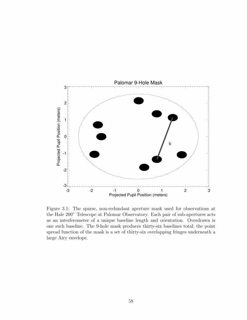
Palomar 9-Hole Mask
-3 -2 -1 0 1 2 3Projected Pupil Position (meters)
-3
-2
-1
0
1
2
3
Pro
jecte
d P
up
il P
ositio
n (
me
ters
)
b
Figure 3.1: The sparse, non-redundant aperture mask used for observations atthe Hale 200” Telescope at Palomar Observatory. Each pair of sub-apertures actsas an interferometer of a unique baseline length and orientation. Overdrawn isone such baseline. The 9-hole mask produces thirty-six baselines total; the pointspread function of the mask is a set of thirty-six overlapping fringes underneath alarge Airy envelope.
58
Fourier component, proportional to the square of the total flux in the image. We
refer to the spots to the left or right of center as splodges; they show that the single
baseline interferometer allows the transmission and measurement of two islands of
spatial frequencies, centered at ~u = ±~b/λ. Because the source is a real valued
function, the power spectrum is point symmetric and these two splodges contain
the same information. Generally, we concern ourselves with the spatial frequency
at the center of each splodge only, and only these must be non-redundant.
The van Cittert-Zernike theorem connects this measurement to a single Fourier
component of the source brightness distribution, i.e., the complex visibility. More
generally, the phase and amplitude of the fringe produced by an interferometer of
baseline ~b are equal to the amplitude and phase of complex visibility at spatial
frequency ~u = ~b/λ. In this way, imaging through an interferometry or aperture
mask probes specific spatial frequencies of the image brightness.
Pupil-Plane Wavefront Phase Errors Produce Visibility Phase Errors
Consider an observation through a perturbed but static two-dimensional phase
screen, φ(~x). By design, the phase variance across each sub-aperture is generally
small enough so that the sub-aperture wavefront can be considered partially co-
herent. The baseline extends up to the full diameter of the telescope and so the
difference between the mean phase of each of the two sub-apertures may be quite
large.
Pupil-plane phase errors cause the fringes to shift laterally in the image. A
lateral shift, in turn, means that the phase of the fringe as measured relative
to some reference point has shifted. The phase shift of the fringe matches the
difference between the mean phases of each of the sub-apertures (Figure 3.3). This
59
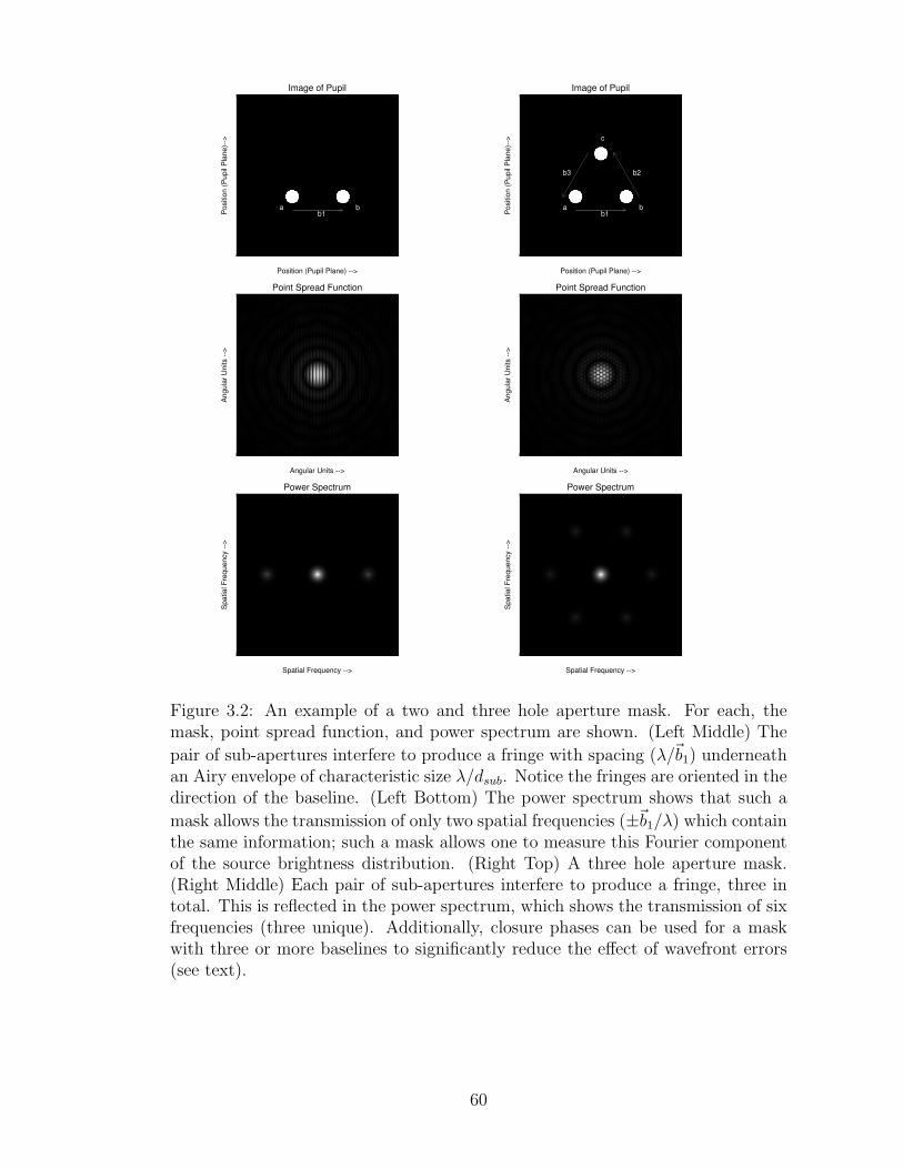
Position (Pupil Plane) -->
Po
sitio
n (
Pu
pil
Pla
ne
)-->
Image of Pupil
a bb1
Position (Pupil Plane) -->
Po
sitio
n (
Pu
pil
Pla
ne
)-->
Image of Pupil
a b
c
b1
b2b3
Angular Units -->
An
gu
lar
Un
its -
->
Point Spread Function
Angular Units -->
An
gu
lar
Un
its -
->
Point Spread Function
Spatial Frequency -->
Sp
atia
l F
req
ue
ncy -
->
Power Spectrum
Spatial Frequency -->
Sp
atia
l F
req
ue
ncy -
->
Power Spectrum
Figure 3.2: An example of a two and three hole aperture mask. For each, themask, point spread function, and power spectrum are shown. (Left Middle) The
pair of sub-apertures interfere to produce a fringe with spacing (λ/~b1) underneathan Airy envelope of characteristic size λ/dsub. Notice the fringes are oriented in thedirection of the baseline. (Left Bottom) The power spectrum shows that such a
mask allows the transmission of only two spatial frequencies (±~b1/λ) which containthe same information; such a mask allows one to measure this Fourier componentof the source brightness distribution. (Right Top) A three hole aperture mask.(Right Middle) Each pair of sub-apertures interfere to produce a fringe, three intotal. This is reflected in the power spectrum, which shows the transmission of sixfrequencies (three unique). Additionally, closure phases can be used for a maskwith three or more baselines to significantly reduce the effect of wavefront errors(see text).
60
also follows if directly apply Fourier Optics to calculate the complex visibility after
the wavefront has propagated through a phase screen (See Equation A.10). The
measured complex visibility after propagation through the phase screen, V’(~b),
given the true complex visibility of the source, V(~b), is:
V ′(~b) = V (~b)
∫sub−
aperture 1
d~x ei[φ(~x+~b)−φ(~x)]. (3.4)
The integral is carried out in the two-dimensional pupil plane. Taylor expanding
the exponential in this equation yields:
V ′(~b) = V (~b)
∫d~x
[1 + i[φ(~x+~b)− φ(~x)]− 1
2[φ(~x+~b)− φ(~x)]2 +O(iφ3)
].
(3.5)
where all integrals are assumed to be over sub-aperture one. The first order terms
shift the phase of the complex visibility; performing the integral simply averages
the phases above each of the sub-apertures. The measured visibility phase, Φ′~b is:
Φ′~b = Φ~b + φ2 − φ1 to first order in φ, (3.6)
where that φ1 and φ2 are the average wavefront phase error above sub-apertures 1
and 2, respectively.
The second order terms reduce the visibility amplitude by a factor which de-
pends on the variance of the phase difference between all points separated by a
baseline length, ~b: σ2φ =< [φ(~x +~b) − φ(~x)]2 >. This is an interferometric analog
to the Strehl ratio and the Marechal approximation (Born & Wolf, 1993), and a
more detailed calculation reveals:
|V (~b)| ∼ e−σ2φ/2 ∼ 1− 1
2σ2φ. (3.7)
For the seeing-limited case, the wavefront phase errors arise from Kolmogorov
turbulence. The quantity φ(~x+~b)−φ(~x) is a Gaussian random variable with mean
61
zero and variance of Dφ(|b|) = 6.88(b/r0)5/3. In particular, note that for baselines
longer than b & r0 the phase of V (~b) now contains a noise term with a variance
much larger than 2π radians. These baselines correspond to the high-angular
resolution content of the complex visibility.
One is unable to extract complex phase for such baselines. Consider the sig-
nal to noise one obtains from successive averaging of many measurements of the
complex visibility quantity exp(Φ′~b) = exp(Φ~b) exp(iφ1 − iφ2). This expression
is the averaging of a phasor exp(ix) where x is mean zero Gaussian distributed
with some large variance (σ & π radians). Successive averaging of phasors with
large variances never decreases measurement error and does not allow extraction
of any useful information of the underlying signal (Figure 3.4). In other words,
phase information is lost for all baselines longer than r0 in the seeing-limited case.
This highlights the need for more sophisticated methods of extracting the visibility
phase for long baselines. The reward for this diligence is higher resolution imaging.
Adaptive optics systems provide a mechanism for maintaining coherence across
the full aperture, so that the variance Dφ(|b|) asymptotes for long baselines.
Diffraction-limited correction corresponds, roughly, to maintaining this asymptotic
value below π radians. (See Section A.3.)
For both the seeing-limited and adaptive optics cases, using visibility ampli-
tudes requires calibration against changes in wavefront phase variance. Note the
difference between amplitude and phase. An increase in phase variance is reflected
in larger measurement error of visibility phase but changes the measurement mean
of visibility amplitude. Discerning this drop in visibility amplitude to either the
intrinsic brightness distribution or the wavefront variance requires an observation
of a known target under the same wavefront conditions. The level of seeing and
62
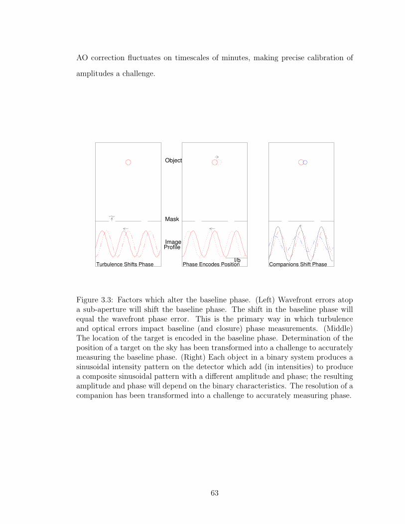
AO correction fluctuates on timescales of minutes, making precise calibration of
amplitudes a challenge.
Turbulence Shifts Phasel/b
Object
Mask
ImageProfile
Phase Encodes Position Companions Shift Phase
Figure 3.3: Factors which alter the baseline phase. (Left) Wavefront errors atopa sub-aperture will shift the baseline phase. The shift in the baseline phase willequal the wavefront phase error. This is the primary way in which turbulenceand optical errors impact baseline (and closure) phase measurements. (Middle)The location of the target is encoded in the baseline phase. Determination of theposition of a target on the sky has been transformed into a challenge to accuratelymeasuring the baseline phase. (Right) Each object in a binary system produces asinusoidal intensity pattern on the detector which add (in intensities) to producea composite sinusoidal pattern with a different amplitude and phase; the resultingamplitude and phase will depend on the binary characteristics. The resolution of acompanion has been transformed into a challenge to accurately measuring phase.
63

Averaging Does Not Decrease Large Phase Errors
0 10 20 30 40# of Measurements
1
10
100
Measure
ment E
rror
after
N M
easure
ments
s = 3 deg
s = 10 deg
s = 30 deg
s = 60 deg
s = 90 deg
s = 120 degs = 180 deg
Figure 3.4: Monte Carlo simulation showing that all signal is virtually unrecov-erable if phase noise is larger than about 150 degrees. Successive averaging ofa Gaussian variable usually reduces its measurement error by N−1/2; this is notthe case for successive averaging of phasors when phase variance is large. Eachdata point shows the measurement uncertainty of the phase of
∑N exp(ix), if x
is a mean-zero Gaussian variable with standard deviations ranging from 3 to 180degrees. If the phase error of x is small, successive averaging leads to an N−1/2
improvement of error after N measurements. As the phase error approaches about150 degrees, averaging is unable to recover that the mean phase is zero after anynumber of measurements by this approach.
64
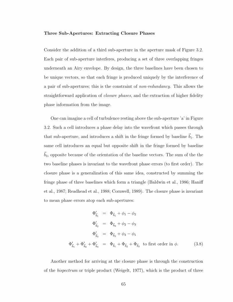
Three Sub-Apertures: Extracting Closure Phases
Consider the addition of a third sub-aperture in the aperture mask of Figure 3.2.
Each pair of sub-aperture interferes, producing a set of three overlapping fringes
underneath an Airy envelope. By design, the three baselines have been chosen to
be unique vectors, so that each fringe is produced uniquely by the interference of
a pair of sub-apertures; this is the constraint of non-redundancy. This allows the
straightforward application of closure phases, and the extraction of higher fidelity
phase information from the image.
One can imagine a cell of turbulence resting above the sub-aperture ’a’ in Figure
3.2. Such a cell introduces a phase delay into the wavefront which passes through
that sub-aperture, and introduces a shift in the fringe formed by baseline ~b1. The
same cell introduces an equal but opposite shift in the fringe formed by baseline
~b3, opposite because of the orientation of the baseline vectors. The sum of the the
two baseline phases is invariant to the wavefront phase errors (to first order). The
closure phase is a generalization of this same idea, constructed by summing the
fringe phase of three baselines which form a triangle (Baldwin et al., 1986; Haniff
et al., 1987; Readhead et al., 1988; Cornwell, 1989). The closure phase is invariant
to mean phase errors atop each sub-apertures:
Φ′~b1 = Φ~b1 + φ1 − φ2
Φ′~b2 = Φ~b2 + φ2 − φ3
Φ′~b3 = Φ~b3 + φ3 − φ1
Φ′~b1 + Φ′~b2 + Φ′~b3 = Φ~b1 + Φ~b2 + Φ~b3 to first order in φ. (3.8)
Another method for arriving at the closure phase is through the construction
of the bispectrum or triple product (Weigelt, 1977), which is the product of three
65
complex visibilities:
B123 = V (~b1)V (~b2)V (~b3) = |V~b1 ||V~b2||V~b3|ei(Φ~b1
+Φ~b2+Φ~b3
)(3.9)
The argument of the bispectrum is the closure phase (Roddier, 1986).
Regardless of the size of the sub-aperture, closure phases remove the first order
term of wavefront noise; the error in closure phases is third order in wavefront
error. This calculation is conducted in more depth and recast by decomposing the
sub-aperture wavefronts into Zernike modes in Section 5.10. Its conclusion is that
mean wavefront phase differences between sub-apertures have no impact on closure
phases. Instead, only wavefront variation within a sub-aperture leads to closure
phase errors. This is the key utility of closure phases. Last section discussed
that phase variations grow for longer separations, and the phase variation across
a baseline will always be larger than the phase variation within a sub-aperture.
In the seeing-limited case, closure phases allow extraction of phase information.
The variance of closure phases (the argument of the bispectrum) is much smaller
than the variance of visibility phases, and so successive measurement of the bis-
pectrum allows meaningful extraction of the closure phase (c.f. Figure 3.4). With
adaptive optics, closure phases still rejects a substantial portion of phase errors,
and will be more precisely measured.
Closure phases have important consequences for calibration and quasi-static
wavefront phase errors. The direct imaging point spread function changes shape
significantly as seeing or adaptive optics performance changes and quasi-static
speckle locations are sensitive to quasi-static wavefront errors across the entire
pupil. By comparison, the transfer function for the closure phase does not depend
on seeing or adaptive optics performance (except in the sense that they introduce
phase errors), and so it is not necessary to calibration closure phases to seeing
66

effects (Weigelt, 1977). Closure phases also only lead to miscalibration if the
quasi-static wavefront within each sub-aperture changes. The magnitude of quasi-
static changes on sub-aperture scales is smaller and slower, and so closure phases
are more robust to quasi-static errors as well.
Hence, closure phases are a powerful method for obtaining higher precision mea-
surements of the Fourier content of the source brightness, particularly for the long
baselines which are most important for high angular resolution. As an example,
Figure 3.5, shows that the variation of closure phases from exposure to exposure
is often an order of magnitude lower than the variance of each individual baseline
phase, even when adaptive optics are providing diffraction-limited correction.
An array of N sub-apertures contains N(N-1)/2 possible baselines. If the base-
lines are non-redundant, each probes the complex visibility at a different spatial
frequency. Closure triangles can be constructed from any three sub-apertures, i.e.,
by drawing the triangle which connects them, of which there are N(N-1)(N-2)/3!
possible triangles. However, the set of triangles is not linearly independent. (This
must be so. Because the closure phases are derived from baseline phases, one
cannot arrive at more independent information after constructing closure phases.)
There are (N-1)(N-2)/2 linearly independent closure phases (or bispectrum) (Read-
head et al., 1988).
Because there are fewer closure phases than baselines, it is not possible to
reverse this procedure. One cannot uniquely determine the baseline phases from
the closure phases. The closure phase information cannot be uniquely inverted
to an image (by conversion to baseline phases and inverse Fourier transform).
Further assumptions are necessary, for instance, that the image is positive valued
and of finite extent. (See, for example, the CLEAN algorithm (Hogbom, 1974)
67
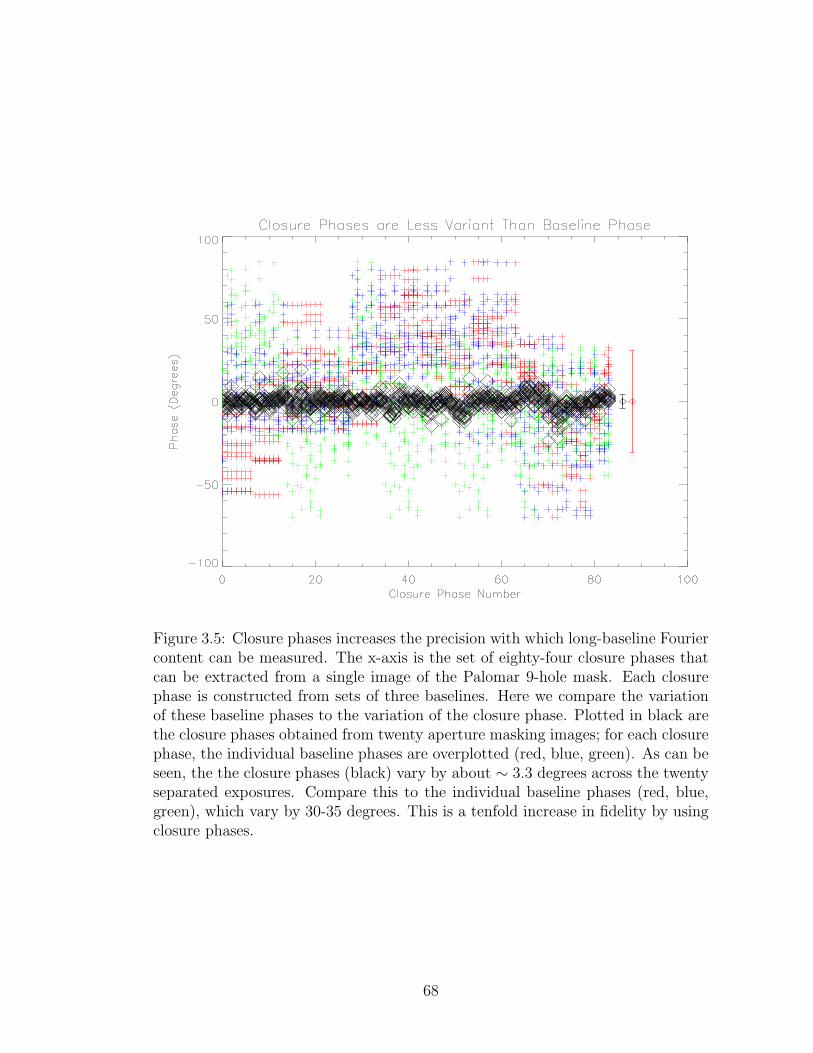
Figure 3.5: Closure phases increases the precision with which long-baseline Fouriercontent can be measured. The x-axis is the set of eighty-four closure phases thatcan be extracted from a single image of the Palomar 9-hole mask. Each closurephase is constructed from sets of three baselines. Here we compare the variationof these baseline phases to the variation of the closure phase. Plotted in black arethe closure phases obtained from twenty aperture masking images; for each closurephase, the individual baseline phases are overplotted (red, blue, green). As can beseen, the the closure phases (black) vary by about ∼ 3.3 degrees across the twentyseparated exposures. Compare this to the individual baseline phases (red, blue,green), which vary by 30-35 degrees. This is a tenfold increase in fidelity by usingclosure phases.
68

and the Maximum Entropy Method (Gull & Skilling, 1984)). Alternatively, by
parameterizing the image structure - such as describing a binary target only by
separation, orientation, and contrast - one can make tractable inferences of the
source distribution without producing an image.
Baseline and Sub-Aperture Redundancy
A critical requirement of the non-redundant aperture masking design is that each
pair of sub-aperture creates a unique interferometric baseline (Haniff et al., 1987;
Roddier, 1986). Readhead et al. (1988) provides an extensive treatment of the
impact of redundant baselines for seeing-limited aperture masking. When two or
more baselines contribute to the same spatial frequency, the power adds partially
incoherently depending on the phase difference of each contributing baselines. A
random phase component will be introduced into the resulting spatial frequency
phase which cannot be removed by closure phases; this component is termed re-
dundancy noise. In completely analogous fashion, temporal variations of the non-
redundant baseline phase during a single exposure create temporal redundancy
which also give rise to closure phases errors.
The mask cannot be entirely non-redundant. The finite sub-aperture size means
that baselines are redundant at least within a sub-aperture. The terminology of
Readhead et al. (1988) defines redundant baselines slightly more critically, referring
specifically to any two pairs sub-apertures (i.e., any two baselines) which differ in
phase by more than one radian r.m.s., in other words, any two baselines which are
totally incoherent. Given the properties of Kolmogorov turbulence, atmospheric
phase screens decorrelate on length scales larger than the Fried parameter and
timescales longer than the atmospheric coherence time. With uncorrected ob-
69
serving, forbidding incoherent baseline redundancy restricts sub-aperture sizes to
smaller than the Fried parameter and exposure times shorter than the atmospheric
coherence time.
Adaptive optics removes both constraints since good correction supplies a sta-
ble, mostly coherent wavefront across the full aperture. Since each baseline is
redundant within the sub-aperture, closure phase errors still arise due to the re-
maining spatial incoherence within the sub-aperture. This lends itself to a defi-
nition of redundant baselines which includes any partially coherent baselines, not
just those which are fully incoherent. In short, with sub-aperture scale correc-
tion provided by the AO system, sub-aperture redundancy noise is largely, but
not entirely, removed (Tuthill et al., 2006). The interplay between quasi-static
wavefront errors and sub-aperture redundancy almost certainly sets the ultimate
limits one can achieve with current NRM experiments. In particular, a study of
sub-aperture redundancy noise necessitates a mathematical treatment more exact
than the useful models of Readhead et al. (1988). Such models are provided, as well
as a detailed treatment of sub-aperture redundancy noise for NRM with adaptive
optics in Section 5.10 of Chapter 5.
3.2 Observing Binaries with an Aperture Mask
3.2.1 Closure Phase Signal
Aperture masking observations sample Fourier components of the source bright-
ness. Closure phases are constructed because they permit higher fidelity measure-
ments of this Fourier information. While various techniques exist to revert closure
70

phases back into an image, it is advantageous to use the inherent structure of the
binary to build a parameterized model that can be fit directly to the closure phase
data.
Consider two different source distributions: a single, unresolved star and a re-
solvable binary of two unresolved stars. The binary can be described by three
parameters: separation, |~ρ| (typically measured in milli-arcseconds); position an-
gle, θ, the azimuthal angle measured from celestial north; and contrast ratio, r(λ),
the wavelength dependent ratio of secondary brightness to primary brightness with
r < 1. We may also include the (off-axis) position of the target on the sky, ~α, mea-
sured in the same angular units as the binary separation. Closure phase (and
visibility amplitude) are invariant to absolute target position, but baseline phases
are not. Given the known brightness distribution of each source, we can calculate
the complex visibility directly:
Isingle(~r) = δ(~r − ~α)
Vsingle(~b) = eπi~b·~α/λ
|Vsingle| = 1.0
φv = π~b · ~α/λ
Ibinary(~r) = δ(~r + ~ρ/2− ~α) + r δ(~r − ~ρ/2− ~α)
Vbinary(~b) = eπi~b·~α/λ e
πi~b·~ρ/λ + r e−πi~b·~ρ/λ
1 + r
|Vbinary| =1 + r2 + 2r cos(2π~b · ~ρ/λ)
1 + r
φv = π~b · ~α/λ+ arctan
[r sin(2π~b · ~ρ/λ)
1 + r cos(2π~b · ~ρ/λ)
]
Closure phases are constructed using baseline triplets which form closed trian-
gles. This constrains the three baselines such that ~b1 +~b2 +~b3 = 0. Equivalently,
each closure triangle can be specified by two baselines, with ~b3 = −~b1 −~b2. Using
this constraint, we can derive an analytic expression for the closure phases of single
71
and binary systems:
Φ(~b1,~b2) = φv(~b1) + φv(~b2) + φv(−~b1 −~b2)
Φsingle(~b1,~b2) = 0
Φbinary(~b1,~b2) = arctan
[r sin(2π~b1 · ~ρ/λ)
1 + r cos(2π~b1 · ~ρ/λ)
]+ arctan
[r sin(2π~b2 · ~ρ/λ)
1 + r cos(2π~b2 · ~ρ/λ)
]
− arctan
[r sin(2π(~b1 +~b2) · ~ρ/λ)
1 + r cos(2π(~b1 +~b2) · ~ρ/λ)
](3.10)
From Equation 3.10 it is clear that by measuring the deviations of the closure
phases from zero one can infer the presence of a companion. Thus, instead of in-
verting the closure phases to form an image, we can similarly complete a parameter
search to find the modeled binary that best fits the measured closure phases. This
approach of forward-modeling can be extended for any target whose brightness
distribution can be modeled by a small number of parameters (e.g., imaging of
debris disks or multiple systems).
By the dot product in Equation 3.10, ~b · ~ρ, we see that baselines are insensitive
to binaries oriented perpendicular to the baseline. For this reason, aperture masks
must be constructed to sample many spatial frequencies spanning all orientations
and a wide range of separations.
Figure 3.6 illustrates the phases one would measure as a function of baseline
for the detection of a 2:1 contrast binary separated by 150 mas using the Palomar
9-hole aperture mask. The middle rows show the target phase as a function of
baseline, overplotted by the thirty-six spatial frequencies sampled by the Palomar
mask. The uniform coverage of the Palomar mask at a full range of orientations and
separations ensures sensitivity to companions at all separations and orientations.
The bottom row shows the baseline-phase relation collapsed to one dimension. The
companion induces a phase offset of up to 30 degrees; with typical measurement
72
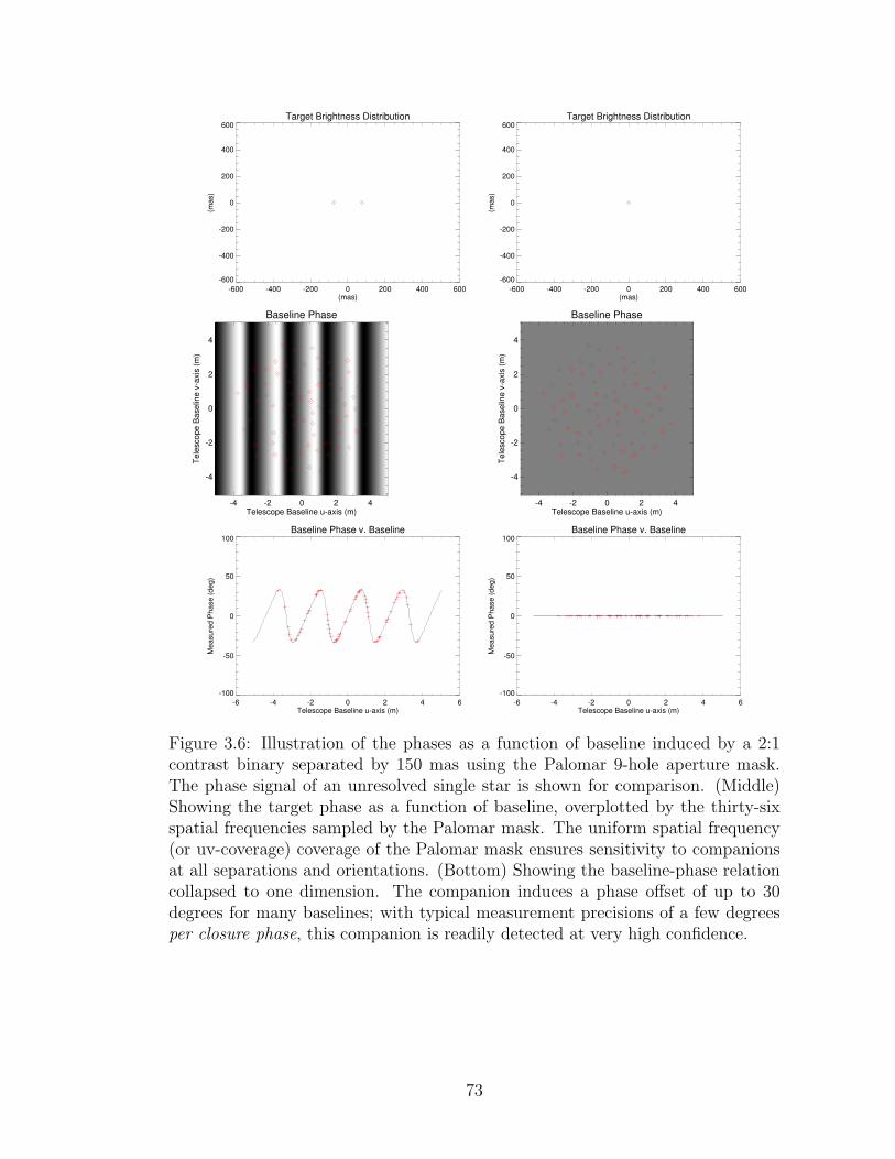
Target Brightness Distribution
-600 -400 -200 0 200 400 600(mas)
-600
-400
-200
0
200
400
600
(mas)
Target Brightness Distribution
-600 -400 -200 0 200 400 600(mas)
-600
-400
-200
0
200
400
600
(mas)
-4 -2 0 2 4Telescope Baseline u-axis (m)
-4
-2
0
2
4
Te
lesco
pe
Ba
se
line
v-a
xis
(m
)
Baseline Phase
-4 -2 0 2 4Telescope Baseline u-axis (m)
-4
-2
0
2
4
Te
lesco
pe
Ba
se
line
v-a
xis
(m
)
Baseline Phase
Baseline Phase v. Baseline
-6 -4 -2 0 2 4 6Telescope Baseline u-axis (m)
-100
-50
0
50
100
Measure
d P
hase (
deg)
Baseline Phase v. Baseline
-6 -4 -2 0 2 4 6Telescope Baseline u-axis (m)
-100
-50
0
50
100
Measure
d P
hase (
deg)
Figure 3.6: Illustration of the phases as a function of baseline induced by a 2:1contrast binary separated by 150 mas using the Palomar 9-hole aperture mask.The phase signal of an unresolved single star is shown for comparison. (Middle)Showing the target phase as a function of baseline, overplotted by the thirty-sixspatial frequencies sampled by the Palomar mask. The uniform spatial frequency(or uv-coverage) coverage of the Palomar mask ensures sensitivity to companionsat all separations and orientations. (Bottom) Showing the baseline-phase relationcollapsed to one dimension. The companion induces a phase offset of up to 30degrees for many baselines; with typical measurement precisions of a few degreesper closure phase, this companion is readily detected at very high confidence.
73
precisions of a few degrees per closure phase, this companion is readily detected at
very high confidence.
3.2.2 Robust Measurement of Binary Parameters and
Confidence Intervals
Unlike the detection of a companion by traditional direct imaging, in which the
companion can be resolved by visual inspection of the image, the detection of a faint
or close companion by aperture masking rests purely on achieving a statistically
significant fit of a model to data. In many of the most interesting cases, this
detection cannot be corroborated by other methods.
In this chapter we present the basic method for calibrating and fitting clo-
sure phase data, which motivates the creation of a new Monte Carlo method for
determining the strength of these fits.
For concreteness, we will consider data obtained with the Palomar 9-hole mask,
although the method can easily be generalized. As described previously, each im-
age produced by the Palomar 9-hole mask consists of thirty-six overlapping fringes
which, when Fourier transformed yields the amplitude and phase of each trans-
mitted spatial frequency. The amplitudes are usually discarded because they are
highly variable due to seeing variations between target and calibrator observations.
Eighty-four closure phases (or bispectrum) can be constructed from each image,
which are then averaged over the set of images and standard deviations are cal-
culated. Finally, these averaged are compared to model closure phases of various
binary configurations to determine the likelihood that the target is binary.
74
Determination of Best Fit
Each closure phase measured from each image is the composite of three sources:
the intrinsic signal of the target, which is zero for a single star and non-zero for a
binary; a non-stochastic systematic error component, which may vary from target
to target (e.g. quasi-static wavefront errors ,flexure of the primary mirror after
slewing, etc.), but not during the observation of a single target; and stochastic
noise from various sources such as time-varying wavefront errors, read noise, etc.
We denote the intrinsic signal by Φbinary, the systematic component by βsystem(t),
and the stochastic noise by ξnoise(t,i). The closure phase, k, extracted from a single
image, i, during a single set of images, t, Φk,t,i, is:
Φk,t,i = Φk,binary + βk,system(t) + ξk,noise(i,t). (3.11)
Averaging over the set of images yields
µΦk,t = Φk,binary + βk,system(t), (3.12)
σ2Φk,t
= < ξ2k,noise(i) > . (3.13)
In other words, the systematic contribute introduces an offset from the true value,
and the stochastic noise describes the measurement variance. The systematic com-
ponent βk,system(t) may change from one acquisition to another but is assumed
constant during the observation of a single target.
Typically, one uses the measurement of calibrator (single) stars, with zero in-
trinsic signal (i.e., Φk,binary = 0), to estimate the underlying distribution of sys-
tematic noise. The typical observing mode is to obtain several observations of the
science target, interspersed with observations of calibrator stars. Although the
systematic component cannot be determined exactly because it is itself a random
75
variable, we can compile a composite distribution of βk,system from the several sets
of calibrator observations:
µβk,system = < βk,system(c) > (3.14)
σ2βk,system
= < β2k,system(c) > −µ2
βk,system(3.15)
Here the averages are over the sets of calibrator observations; σ2βk,system
reflects
the variation of the systematic effects as the telescope is moved from one star to
another, etc. For instance, the evolution of quasi-static wavefront errors will cause
the systematic component to vary from one calibrator to the next.
Subtracting the systematic component from the measured closure phases leaves
remaining the intrinsic signal of the target, Φk,binary:
Φk,binary = µΦk,t − µβk,system (3.16)
σ2Φk,t
= < ξ2k,noise(i) > +σ2
βk,system(3.17)
In short, the calibrator closure phases are subtracted from the science target closure
phases, and their errors are added in quadrature. This calibration step is important
for obtaining high contrasts during high signal to noise observations, when the
contribution from systematic noise is on the order of the stochastic noise.
We wish find the three-parameter model binary (separation ρ, orientation θ,
and contrast ratio r) which best fits the calibrated signal, Φk,binary. This is most
readily approached as a χ2 minimization problem by finding the set of noiseless,
modeled binary closure phases Φm(ρ, θ, r) which minimize the quantity:
χ2 =∑k
(Φk,binary − Φk,m(ρ, θ, r))2
σ2Φk,t
(3.18)
There are many alternatives to this approach. For instance, one could use boot-
strapping methods to calculate measurement errors (or measurement likelihood
76
curves) that don’t assume Gaussianity. There could easily be incorporated into a
Monte Carlo algorithm to determine the distribution of best fits. For simplicity,
we will consider the problem as a χ2 minimization problem.
The best-fitting model is that which minimizes the χ2, which we determine by
a combination of gradient search and visual inspection. The parameter errors are
calculated from the curvature of the χ2 surface at the minimum. Calculating the
confidence of this fit, i.e. that this model represents the true target configuration,
is detailed in the next subsection.
Experience has shown that the reduced-χ2 of best fits to even benchmark (i.e.,
known) binaries are typically larger than unity by a factor of one to a few. We take
this as an indication of an unknown systematic error that is not properly accounted
for by our estimate of the systematic component from calibrator measurements, nor
the measurement scatter across the set of images. In these cases, it is typical for us
to artificially scale the closure phase until the reduced χ2 of the best fitting binary
is unity. Further development of the closure phase extraction pipeline may also
indicate a bias towards underestimated errors, but this has not yet been explored.
Binary Detection Confidence
Our null hypothesis, which we wish to test against the binary fit, is that the ob-
served target is a single star, with intrinsic binary phase zero. Following Equation
3.18, the probability of the null model is
χ2null =
∑k
Φk,m(ρ, θ, r)2
σ2Φk,t
. (3.19)
A natural goodness-of-test statistic is to compare the ratio of the data and null
χ2. This is particularly useful for our aperture masking data because its value will
77
not change if errors are scaled (see previous section). This ratio is similar to an
’F-statistic,’ which is the ratio of two reduced χ2 variables and we adopt the same
name:
F = χ2/χ2null (3.20)
The F statistic ranges from 0 to 1; a low F value signifies a strong fit.
Systematic and stochastic noise may at times conspire to mimic a binary signal,
as expressed by a well fitting a binary model, even though the target is a single
star. This is a false alarm event. We, therefore, classify the target fit as statistically
significant only if its F-value small compared to a distribution of F-values obtained
by fitting single stars.
To obtain this probability of false alarm we simulate ten thousand measure-
ments of single stars with identical (u,v)-coverage and noise properties of the can-
didate binary target data. The intrinsic phase of a single star, Φbinary, is zero. For
one measurement, the contribution due to statistical noise is drawn from the mea-
sured distribution of ξk,noise, which typically can be approximated by a Gaussian
distribution with mean zero and its measured standard deviation (σ2Φk,t
). The sys-
tematic contribution, if included, is drawn from a distribution βk,system, compiled
from observations of calibrator (single) stars. An alternative to this method is to
employ bootstrapping for generating simulated datasets using the original data.
Without justification to assume noises are Gaussian, bootstrapping is less biased,
and will automatically preserve all correlations between the data (which are known
to be large for closure phase data).
We then fit the simulated single star data with a three-parameter binary model,
record its ∆χ2 or F statistic, and build a distribution of these variables. The
probability of false alarm, then, is the probability that the goodness-of-fit of a
78
single star is higher than the target data’s goodness-of-fit. The percentage of
single star fits which yield a better fit than the data yields the probability of false
alarm, that claim our data reveals a phantom binary:
pfalse alarm(Φm) = p(Fbest fit to data > Ffits to single stars ) (3.21)
and
detection confidence = 1− pfalse alarm. (3.22)
We consider the target data to reveal a definitive 3-sigma binary detection if the
best-fitting model produces a detection confidence greater than 99.7% (false alarm
probability less than 0.3%). Note that this empirical method is more conservative
than comparing the measured ∆χ2 statistic to an analytical distribution with three
degrees of freedom (Fig. 3.7).
3.2.3 Calculation of Contrast Limits
Whether or not the target is identified as a single star or binary, we are also able to
quantitatively state the highest contrast (dimmest) companion that our technique
would have been capable of identifying with high confidence (99.7%) as a function
of separation. This is, in essence, a statement on the noise characteristics of the
data and the uv-coverage of our mask.
This amounts to asking the following question: Given simulated binary obser-
vations (separation ρ, orientation θ, and contrast ratio r), at what contrast does
our detection confidence drop below 99.7% (or false alarm probability rise above
0.3%)?
79
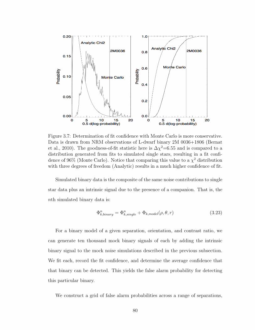
Figure 3.7: Determination of fit confidence with Monte Carlo is more conservative.Data is drawn from NRM observations of L-dwarf binary 2M 0036+1806 (Bernatet al., 2010). The goodness-of-fit statistic here is ∆χ2=6.55 and is compared to adistribution generated from fits to simulated single stars, resulting in a fit confi-dence of 96% (Monte Carlo). Notice that comparing this value to a χ2 distributionwith three degrees of freedom (Analytic) results in a much higher confidence of fit.
Simulated binary data is the composite of the same noise contributions to single
star data plus an intrinsic signal due to the presence of a companion. That is, the
nth simulated binary data is:
Φnk,binary = Φn
k,single + Φk,model(ρ, θ, r) (3.23)
For a binary model of a given separation, orientation, and contrast ratio, we
can generate ten thousand mock binary signals of each by adding the intrinsic
binary signal to the mock noise simulations described in the previous subsection.
We fit each, record the fit confidence, and determine the average confidence that
that binary can be detected. This yields the false alarm probability for detecting
this particular binary.
We construct a grid of false alarm probabilities across a range of separations,
80
orientations, and contrast ratios. For each separation we average over the orien-
tations, and determine the highest contrast ratio i.e., dimmest companion) that
would be detected with 99.7% confidence.
Ideally, we would determine the confidence of each mock binary by searching for
its best fit, recording its F or ∆χ2, and comparing it to the false alarm distribution
of the previous subsection. In practice, using a fitting routine to fit each of these
simulated binaries is computationally slow.
Instead we approximate this process by modifying the false alarm distribution.
We make the assumption that the inserted binary model yields the best fit. Because
we effectively restrict the fitting search to the range of separation, orientations, and
contrast ratios used to generate the mock binaries, we apply the same restriction
to the fitting search that generates the false alarm distribution. We then use
this modified false alarm distribution to determine the confidence of the mock
binary fits. In practice, this approximation produces contrast limits slightly more
conservative than full fitting by about 5-10%.
81
CHAPTER 4
A CLOSE COMPANION SEARCH AROUND L DWARFS USING
APERTURE MASKING INTERFEROMETRY AND PALOMAR
LASER GUIDE STAR ADAPTIVE OPTICS1
4.1 Abstract
We present a close companion search around sixteen known early-L dwarfs using
aperture masking interferometry with Palomar laser guide star adaptive optics.
The use of aperture masking allows the detection of close binaries, corresponding
to projected physical separations of 0.6-10.0 AU for the targets of our survey. This
survey achieved median contrast limits of ∆K ∼ 2.3 for separations between 1.2 -
4 λ/D, and ∆K ∼ 1.4 at 23λ/D.
We present four candidate binaries detected with moderate to high confidence
(90-98%). Two have projected physical separations less than 1.5 AU. This may
indicate that tight-separation binaries contribute more significantly to the binary
fraction than currently assumed, consistent with spectroscopic and photometric
overluminosity studies.
Ten targets of this survey have previously been observed with the Hubble Space
Telescope as part of companion searches. We use the increased resolution of aper-
ture masking to search for close or dim companions that would be obscured by full
aperture imaging, finding two candidate binaries.
This survey is the first application of aperture masking with laser guide star
adaptive optics at Palomar. Several new techniques for the analysis of aperture
1Previously published as Bernat et al. (2010)
82
masking data in the low signal to noise regime are explored.
4.2 Introduction
The mass determinations of stars through binary studies have provided numerous
mass-luminosity benchmarks for the testing and calibration of stellar models. Such
studies have only recently begun for the regime of brown dwarfs.
The empirical calibration of brown dwarf models is generally made more dif-
ficult by the added dependency on age in the mass-luminosity relationship. For
example, an object spectroscopically classified as a late-M dwarf may be a young
brown dwarf or an old star just above the hydrogen burning limit. This broadens
the range of potential physical properties (mass, age, composition) that generate
the same observable spectrum. Conversely, photometry can only very generally re-
veal the objects’ physical properties. Measurements of brown dwarf masses through
the tracking of binary orbits provide the strongest constraints on stellar models,
”mass benchmarks” that reduce the degeneracy of photometric studies even for
targets with unknown ages (Liu et al., 2008). Mass measurements of brown dwarfs
by Konopacky et al. (2010) show systematic discrepancies between models and
measurements; late-M through mid-L systems tended to be more massive than
models predict, while one T dwarf system was less massive than its model predic-
tion. This collection of mass benchmarks grows even more important as brown
dwarf models are extended to infer the masses of directly imaged planets, such
system HR 8799 (Marois et al., 2008).
Binary surveys have also begun to turn up interesting statistical results that
may suggest the brown dwarf binary formation mechanism is different than that for
83
solar type binaries (see Burgasser et al. (2007) for a summary of results from low
mass surveys, including many results presented in this section). Few surveys, how-
ever, have produced results for very low mass binaries, especially those with very
tight separations (. 3.0 AU). This regime of short period binaries is particularly
challenging to achieve with ground-based direct imaging.
While the companion fraction of brown dwarfs is proposed to be low (≈ 15%)
and peaked within a narrow separation range, 3-10 AU (Burgasser et al., 2008),
little conclusive results are known for separations less than 3 AU despite prelimi-
nary evidence that many additional companions are likely to reside at very close
distances (Jeffries & Maxted (2005); Pinfield et al. (2003); Chappelle et al. (2005)).
Over 90% of known very low mass binaries have less than 20 AU (Burgasser
et al., 2007). Competing theories of stellar formation aim to explain the observed
companion statistics of brown dwarfs. As a general trend, stars appear to have
a binary fraction that decreases with mass. This can partly be explained by the
decreased binding energy of lower mass primaries, and thus a maximum binary
separation that decreases as a function of total mass (Reid et al. (2001); Close et al.
(2003)). For very low mass stars, the companion fraction peaks near 3-10 AU, and
exhibits a significant (and statistically significant) drop at separations beyond 20
AU separation. Slightly more than half of known very low mass binaries lay within
this narrow separation range (Burgasser et al., 2007). On the near side of this peak,
the data collected is very likely incomplete, where the necessary resolution (300
mas) stretches the limitations of HST/NICMOS and ground-telescopes with AO
alone. What data has been collected suggests direct imaging may have missed
companions at very close separations.
Spectroscopic, spectral morphology, and Laser Guide Star AO surveys suggest
84
that very tight binaries within 3 AU may be as plentiful as binaries of moderate
separation. Burgasser et al. (2007) has used spectral features of unresolved sources
to indicate composite spectra, implying multiplicity. This technique has suggested
numerous early/mid-L dwarfs with potential mid-T dwarf secondaries and systems
of equal-mass L/T transition objects. Jeffries & Maxted (2005) used sparse radial
velocity data-sets of very low mass systems to predict an additional 17-30% binaries
at separations less than 2.6 AU. Photometric overluminosity studies by Pinfield
et al. (2003) and Chappelle et al. (2005) have also hinted at surprisingly larger
binary fractions (up to 50%) in the Pleiades and Praesepe, though concerns over
membership contamination and the influence of variability limit the conclusiveness
of the results. In each study, with the exception of the Burgasser mid-L/mid-T
systems, very low mass binaries tend towards equal mass pairs (q ∼ 1) at close
separations, just as is the case at moderate separation.
These preliminary results contrast those of previous, observationally complete
surveys that focused on moderate and wide separation binaries. Those surveys
predict that fewer than 3% of very low mass companions sit at separations closer
than 3 AU (Allen, 2007). This discrepancy speaks to the importance of additional,
observationally complete surveys searching for binaries at close separations.
Non-Redundant Aperture Masking (NRM) on 5-10m class telescopes, combined
with LGS AO, allows sub-diffraction limit resolution observations at contrasts high
enough to search for most binaries in this potentially fertile, unresolved region.
The detection of close brown dwarf binaries, with a typical period of 1-2 years,
also allows mass measurements of late-L or T dwarfs, providing particularly valu-
able empirical benchmarks for the study of low mass stellar models. To put into
perspective the dearth of benchmarks, the mass measurements of fifteen very low
85
mass systems (including six with L or T dwarf components) using LGS AO alone
by Konopacky et al. (2010) has tripled the number of very low mass systems with
mass measurements.
In Section 4.3 we describe the sixteen field L-dwarf targets imaged at Palomar
using aperture masking with laser guide star adaptive optics and outline the data
analysis techniques used to determine the binarity of the targets. In Section 4.4, we
present the results of our survey, which operated in the range of 60-320 mas (1.1-8.4
AU @ 18.4 pc, the median distance of our targets). We identify four new candidate
L dwarf-brown dwarf binaries at moderate or high (90-98%) confidence. This
survey achieved median contrast limits of ∆K∼2.3 between 1.2 λ/D and 4 λ/D,
ruling out companions down to approximately .06 M�for old (5 Gyr) systems and
.03 M�for young (1 Gyr) systems. In Section 5.8, we discuss the aperture masking
techniques employed in this paper and present recommendations for future faint
target observations. In Section 4.6, we summarize the results of this survey and
discuss its implications for future companion searches around brown dwarfs.
4.3 Observations and Data Analysis
4.3.1 Observations
We observed our target sample of sixteen field L dwarfs in September and October
2008 with the Palomar Hale 200” telescope (refer to Table 4.1).
Ten of the sixteen targets in this survey have been observed previously as
part of various companion searches using the Hubble Space Telescope (Reid et al.,
86
2006; Bouy et al., 2003). These previous observations were capable of resolving
low contrast or distant (beyond about 300 mas) companions. Aperture masking
complements these previous surveys, extending the detection limits around these
targets to dimmer and closer companions.
Aperture masking observations were obtained using the PHARO instrument
(Hayward et al., 2001), with a 9-hole aperture mask installed in the pupil plane of
the Lyot-stop wheel (Figure 4.1). The longest and shortest baselines, which set the
approximate inner and outer working angle, are 3.94m and 0.71m respectively (58
and 320 mas in K band). We operate to minimize atmospheric and AO variation
during a single image, using PHARO in 256 x 256 sub-array mode with a total of
16 reads (sub-frames) per array reset and 431 ms exposures. Every read was saved
to disk. In post-processing, we discard the first three sub-frames of each exposure
(usually corrupted by detector reset), and combine the remaining sub-frames by
a Fowler sampling algorithm in which later sub-frames are weighed more heavily.
Approximately 300 images (each with 16 sub-reads) were taken in Ks for each
target, for a total integration time of roughly 60-70 minutes per target.
The Palomar laser guide star adaptive optics system (Roberts et al., 2008) pro-
vided the wavefront reference for high order AO correction, while nearby (a few
arc-minutes) field stars were observed contemporaneous to provide tip-tilt correc-
tion.
Aperture masking operates most effectively when exposure times are as short
as possible, but long enough to observe fringes over read noise. The optimal
exposure time depends on the brightness of the targets and the level of correction
provided by the AO system. Poor correction favors shorter exposure times, where
variation of the incoming wavefront quickly degrades the average transmission of
87
long baseline frequencies. For targets brighter than about tenth magnitude, the
read out limited exposure time of the PHARO detector, 431 ms for the 256 x
256 array, is sufficient to observe long baseline fringes. The targets of this survey
are approximately twelfth magnitude, and initial experimentation showed that
short exposures did not consistently provide long baseline fringes. Longer exposure
times (1 minute) faired poorly because variations in correction over the exposure
degraded the average transmission of long baselines below background levels. We
opted to use short exposures and to weigh more heavily in post-analysis those
observations in which long baseline fringes could be seen (see additional discussion
later in this section).
Background subtraction is necessary for targets as faint as L Dwarfs and back-
ground levels were often comparable to the signal levels. In many instances our ob-
servations were background limited. To remove the background in post-processing,
each target was dithered on the 256 x 256 sub-array.
A requirement for obtaining good contrast limits around bright targets is the
contemporaneous observation of calibrator sources: single stars which are nearby
in the sky and similar in near-infrared magnitudes and colors. This calibration
is necessary to remove non-stochastic phase errors introduced by primary mirror
imperfections and other non-equal path length errors. This error can be on the
order of one to a few degrees, comparable to the measurement scatter of the closure
phases for bright targets. For brighter targets, the typical observing mode is to
obtain several observations of the science target, interspersed with observations
of calibrator stars. However, the lengthy time of acquisition for the laser guide
star AO system made this method inefficient for this survey. Furthermore, the
measurement scatter for the faint targets of this survey were much larger than the
88
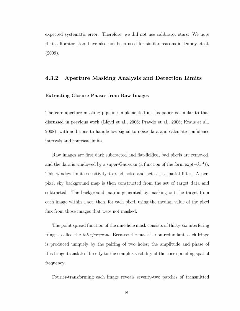
expected systematic error. Therefore, we did not use calibrator stars. We note
that calibrator stars have also not been used for similar reasons in Dupuy et al.
(2009).
4.3.2 Aperture Masking Analysis and Detection Limits
Extracting Closure Phases from Raw Images
The core aperture masking pipeline implemented in this paper is similar to that
discussed in previous work (Lloyd et al., 2006; Pravdo et al., 2006; Kraus et al.,
2008), with additions to handle low signal to noise data and calculate confidence
intervals and contrast limits.
Raw images are first dark subtracted and flat-fielded, bad pixels are removed,
and the data is windowed by a super-Gaussian (a function of the form exp(−kx4)).
This window limits sensitivity to read noise and acts as a spatial filter. A per-
pixel sky background map is then constructed from the set of target data and
subtracted. The background map is generated by masking out the target from
each image within a set, then, for each pixel, using the median value of the pixel
flux from those images that were not masked.
The point spread function of the nine hole mask consists of thirty-six interfering
fringes, called the interferogram. Because the mask is non-redundant, each fringe
is produced uniquely by the pairing of two holes; the amplitude and phase of
this fringe translates directly to the complex visibility of the corresponding spatial
frequency.
Fourier-transforming each image reveals seventy-two patches of transmitted
89
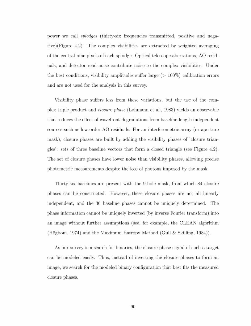
power we call splodges (thirty-six frequencies transmitted, positive and nega-
tive)(Figure 4.2). The complex visibilities are extracted by weighted averaging
of the central nine pixels of each splodge. Optical telescope aberrations, AO resid-
uals, and detector read-noise contribute noise to the complex visibilities. Under
the best conditions, visibility amplitudes suffer large (> 100%) calibration errors
and are not used for the analysis in this survey.
Visibility phase suffers less from these variations, but the use of the com-
plex triple product and closure phase (Lohmann et al., 1983) yields an observable
that reduces the effect of wavefront-degradations from baseline-length independent
sources such as low-order AO residuals. For an interferometric array (or aperture
mask), closure phases are built by adding the visibility phases of ’closure trian-
gles’: sets of three baseline vectors that form a closed triangle (see Figure 4.2).
The set of closure phases have lower noise than visibility phases, allowing precise
photometric measurements despite the loss of photons imposed by the mask.
Thirty-six baselines are present with the 9-hole mask, from which 84 closure
phases can be constructed. However, these closure phases are not all linearly
independent, and the 36 baseline phases cannot be uniquely determined. The
phase information cannot be uniquely inverted (by inverse Fourier transform) into
an image without further assumptions (see, for example, the CLEAN algorithm
(Hogbom, 1974) and the Maximum Entropy Method (Gull & Skilling, 1984)).
As our survey is a search for binaries, the closure phase signal of such a target
can be modeled easily. Thus, instead of inverting the closure phases to form an
image, we search for the modeled binary configuration that best fits the measured
closure phases.
90
Figure 4.1: The aperture mask inserted at the Lyot Stop in the PHARO detector.Insertion of the mask at this location is equivalent to masking the primary mirror.
Figure 4.2: Interferogram and power spectrum generated by the aperture mask.(Left) The interferogram image is comprised of thirty-six overlapping fringes, onefrom each pair of holes in the aperture mask. (Right) The Fourier transformof the image shows the thirty-six (positive and negative) transmitted frequencies.(Right, inset and overlay) Closure phases are built by adding the phases of ’closuretriangles’: sets of three baseline vectors that form a closed triangle.
91
Typical Results on Bright Targets
Aperture masking with natural guide star adaptive optics has been employed dur-
ing numerous near infrared surveys on the Palomar and Keck telescopes. (For
mass determinations made through orbit tracking see Lloyd et al. (2006); Ireland
et al. (2008); Martinache et al. (2007, 2009) and Dupuy et al. (2009), and Kraus
et al. (2008) for an extensive survey of Upper Scorpius.) Aperture masking has
also recently begun usage in conjunction with Keck laser guide star adaptive optics
(Dupuy et al., 2009)).
The observation of bright targets (Ks . 9), such as nearby early-M dwarfs,
with an aperture mask enables the detection of companions of contrast up to 150:1
(∆Ks ∼ 5.5) at the formal diffraction limit and 20:1 (∆Ks ∼ 3.3) at 23λ/D in at
Palomar.
In this regime, non-stochastic phase errors introduced by the optical pipeline
dominate closure phase errors, as well as background flux, wavefront residuals of
the adaptive optics system, and achromatic smearing of the fringes. Typically,
these sources contribute errors on the order of one degree after calibration.
Noise Properties of Dim Targets
For each star image, of which we have approximately 300 for each star, we extract
closure phases.
Because our targets are faint and exposure times are short, detector read-outs
contribute significant noise in the phase and amplitude of the complex visibilities
and bispectrum. Amplitudes are particularly susceptible to calibration errors.
92
Even during high signal to noise conditions, amplitudes have been seen to fluctuate
by up to 100%, and are not directly used for fitting to model binaries. However,
closure phase data show a clear improvement in per-measurement signal to noise
for increasing amplitude. That is, bispectrum with the largest amplitude tend to
have the highest fidelity closure phases. In order to pare off bad data and weigh
higher signal to noise measurements more heavily, we empirically estimate the
relationship between amplitude and closure phase fidelity (Figure 4.3).
This relationship is estimated by binning the set of closure phase data by am-
plitude and calculating the standard deviation of each bin. As already described,
as the average amplitude within a bin increased, the standard deviation within
the bin decreased. To first approximation, this estimates the relationship between
amplitude and closure phase fidelity.
The noisiest bins often show closure phase errors approaching 180◦. Because
the closure phase is inherently a measurement of the bispectrum phasor, there
is a 360◦ ambiguity in the measurement of closure phase. Furthermore, even if
the underlying noise source is Gaussian distributed, the distribution of measured
closure phases approaches a uniform distribution when the standard deviation
of the noise source is larger than about 180◦. Direct calculation of the root mean
squared deviation under represents the variance of the underlying noise source; the
calculation of the mean depends on the choice of angle zero-point. The variation
within one bin was at times large enough to motivate alternative methods for
averaging bispectrum data.
We adopt a maximum likelihood method to calculate the standard deviations
of bins and overall closure phase mean. We presume the closure phases in each bin
are drawn from a wrapped normal distribution1. The standard deviation is varied
93

to maximize the likelihood of the data in the bin. The same mean is used for every
bin, and the mean which maximizes the likelihood of the entire data set is data
set’s overall mean. This allows bins to take arbitrarily large standard deviations;
a wrapped normal distribution with large standard deviation converges towards a
uniform distribution. For bins dominated by read-noise or very low signal to noise,
this method accurately estimates very large standard deviations and translate that
into very low weighting for the bin. The overall errors of closure phase sets ranged
between 6-15 degrees. In addition, this method of paring off bad data typically
reduced errors by a factor of two over other methods.
Even after employing this data paring, some sets of closure phase data contained
so much noise that no reliable signal could be discerned. In this case, the closure
phase was removed from the set of eighty-four closure phases further analyzed.
For some targets, up to half of the closure phases triangles were removed. In these
circumstances, the uv-coverage of the data drop allowed the possibility of model
aliasing: i.e., that multiple binary configurations yield similar closure phase sets
and each fit the data equally well. When previous observations of the target were
available, we used this information to rule out unlikely fits. When not, we list all
fits to the data.
Finally, non-stochastic errors are typically on the order of one to a few degrees.
This contribution is much smaller than the statistical error, and as such overall
best fits of our data changed very little whether or not we attempted to calibrate
out this component.
1The wrapped normal distribution is the probability distribution function of the wrappedvariable θ ≡ x mod 2π, given by pw(θ) =
∑p(θ + 2πk), where p is the unwrapped probability
of the unwrapped variable x. The sum is over integer values of k from −∞ to ∞. The wrappednormal distribution, denoted by WN is, WN(θ) ≡ 1√
2πσ2
∑exp[−(θ−µ−2πk)2
2σ2 ], with the samesummation limits.
94
Modeling the Binary Fit, and the Calculation of Confidence and Con-
trast Limits
For each target, we attempted to fit the observed closure phases with a three-
parameter binary model (separation ρ, orientation θ, and contrast ratio r > 1).
The best fitting model is the one which maximized the overall likelihood of the data.
Errors in the parameters are calculated from the curvature of the log-likelihood
surface at its maximum.
The strength of our fits were determined by comparing the increase in log-
likelihood, ∆ logL, between a single star fit and a binary star fit for our real data
set as compared to many simulated data sets of single stars. If the real data set
has a much higher value of ∆ logL than the simulated data sets, we regard the
real data set to be indicative of a binary star. (For purely Gaussian noise, ∆ logL
is equivalent to ∆χ2.)
We simulate measurements of single stars with identical noise properties and
uv-coverage of the candidate binary target. The measured closure phases of a single
star is the sum of three sources: the intrinsic signal of the target, which is zero
for a single star; noise fluctuations from various sources which are described by
the standard deviations measured on the target; and a non-stochastic systematic
error component, which we assume is negligible compared to the stochastic noise of
these targets. (As a check, we also estimated the typical systematic contribution
from the measured signal of eight survey targets whose best fits indicated high
likelihood for being single stars. Including this component to simulate single stars
had little effect on the overall confidence measurements.)
From this information, we generate ten thousand mock measurements of single
95
stars. To each, we fit the three-parameter binary model, record the ∆ logL, and
build a distribution of ∆ logL that result from single star observations.
Comparing the value of ∆ logL of the data’s fit to the simulated distribution
yields the probability of false alarm: the probability that our apparent binary fit
is an observation of a single star co-mingled with noise. The confidence that our
target is binary is one minus this false alarm probability.
To calculate our contrast limits, we first add model binary signals to the sim-
ulated single star data. These mock binary signals span a range of separations,
orientations, and contrast ratios. We fit each, determine the fit confidence, and
determine, for a given separation, the highest contrast ratio (i.e. dimmest com-
panion) that would be detected with 99.5% confidence (false alarm probability of
.005). These calculations are discussed in more detail in the Section ?? of the
previous Chapter.
Calculation of Bayes’ Factors
As an alternative to confidence measure presented in the previous subsection, our
group also applied bayesian methods to calculate the Bayes’ Factor of each fit, i.e,
the odds by which our data favors binary models.
Using Bayesian comparison, the binary hypothesis is tested by contrasting two
probabilities: that the data set would arise from a binary target observation, and
that the set would arise from a single star observation. Expressed mathematically,
this is:
96
Pr( binary | data )
Pr( single | data )=
Pr( star is binary )
Pr( star is single )
Pr( data | binary )
Pr( data | single ). (4.1)
The first term on the right hand side is an attribute of the survey population
– it is the ratio of the companion fraction to one minus the companion fraction –
and is independent on the data.
The second term is the Bayes’ Factor, representing the odds by which the data
favors one hypothesis over the other. These probabilities are marginalized (and
integrated) over the binary parameters. Whereas the maximum likelihood method
searches out the set of parameters that maximizes the likelihood of the data, the
Bayesian approach averages over the parameters.
Bayes′ Factor =Pr( binary | data )
Pr( single | data )(4.2)
=
∫Pr(ρ| bin.)Pr(θ| bin.)Pr(r| bin.)L(data|ρ, θ, r)
L(data | single)(4.3)
The quantities Pr(ρ|binary), Pr(θ|binary), Pr(r|binary) refer to distributions
of the companion separation, orientation, and contrast ratio as they are presumed
known prior to our observation. These distributions for very low mass primaries
are themselves ongoing topics of debate and limited by observational incomplete-
ness, particularly in the separation regime of our survey. (For a current review
of separation and mass ratio distributions derived through observational studies,
the reader is invited to view Burgasser et al. (2007).) Allen (2007) quantifies the
underlying companion distributions from the currently available data. We ulti-
mately chose to use blind prior distributions (known as Jeffreys’ priors). These
97
distributions are uniform for separation and log-uniform for contrast ratio. We
compare this choice to the Allen priors and discuss its implications.
Our survey focuses on close binaries; our observations probe between roughly
1 and 8 AU for seventy five percent of our L dwarf targets. Allen (2007) concludes
that the (physical) separation of companions can be characterized by a log-normal
distribution which peaks at 7.2+1.1−1.7 AU with a 1σ width of roughly 11+∼2
−∼3 AU. This
uncertainty in the peak and width contributes noticible variability of the resulting
distribution at the separations we consider (see Figure 4.4). One characteristic
unifying the span of distributions, however, is that companions closer than ∼ 2
AU are less likely by up to an order of magnitude. The is due in part to describing
the distribution as a log-normal functional. This choice is motivated by the sharp
drop in companion fraction observed outward of about 10 AU, and by assuming a
similar drop shortward of a few AU, where observational data is incomplete. As
Allen states, this result is derived without well-defined searches for companions
at close separations, and the preliminary results of the Jeffries & Maxted (2005)
and Basri & Reiners (2006) surveys potentially indicate the presence of a larger
number of close binaries. We use a uniform prior to avoid the bias of the Allen
priors, keeping in mind that companions with high Bayes’ factor at less than 2 AU
could indicate observational evidence of close companions yet may also be biased
towards undue significance.
Observational surveys of very low mass systems show a tendency towards equal
mass binaries (q ∼ 1) (Burgasser et al., 2007; Reid et al., 2006; Allen, 2007).
The distribution of mass ratios has been roughly characterized by a power law,
p(q) ∝ qγ, with γ ∼ 2 − 4 depending on the survey. The large exponent of this
distribution indicates that low mass ratio (low q) systems are highly unlikely (and
98
rare). Transforming this to a distribution of broad-band contrast ratios (r, with
r > 1) requires assumptions about target age distributions, bolometric luminosity
corrections, and mass-luminosity models (see Allen et al. (2005, 2003) for these
assumptions applied to field stars). We wish our prior distribution not depend so
highly on these assumptions and rather rely on a few basic assumptions.
The rapid drop of the L dwarf mass-luminosity relation (i.e., halve the mass of
the star and its luminosity drops by much more) implies that ratios of contrast are
larger than ratios of mass, and that contrast ratios still favor unity (i.e., p(r) ∝
(1/r)γ with 0 < γ . 2 − 4). The blind prior for a scale independent quantity
like contrast ratios is p(r) ∝ 1/r which, conveniently, has the desired properties.
It is worth noting that Allen (2007, Fig. 14) carries out the transformation from
mass ratio to contrast ratio, finding a distribution that follows roughly p(r) ∝
1/(r log r) for contrasts down to below 100:1.
Finally, the same methods can be applied to calculate posterior distributions for
ρ, θ, and r for each data set. For a data set with a single best fit, this distribution
yields a p.d.f. describing the best fitting parameters. The parameter values and
errors quoted in this paper are those derived from maximum fit likelihood, as
discussed in the previous subsection, and are not drawn from Bayesian posteriors.
However, we calculate the posterior distributions to assure both methods give
comparable results.
99
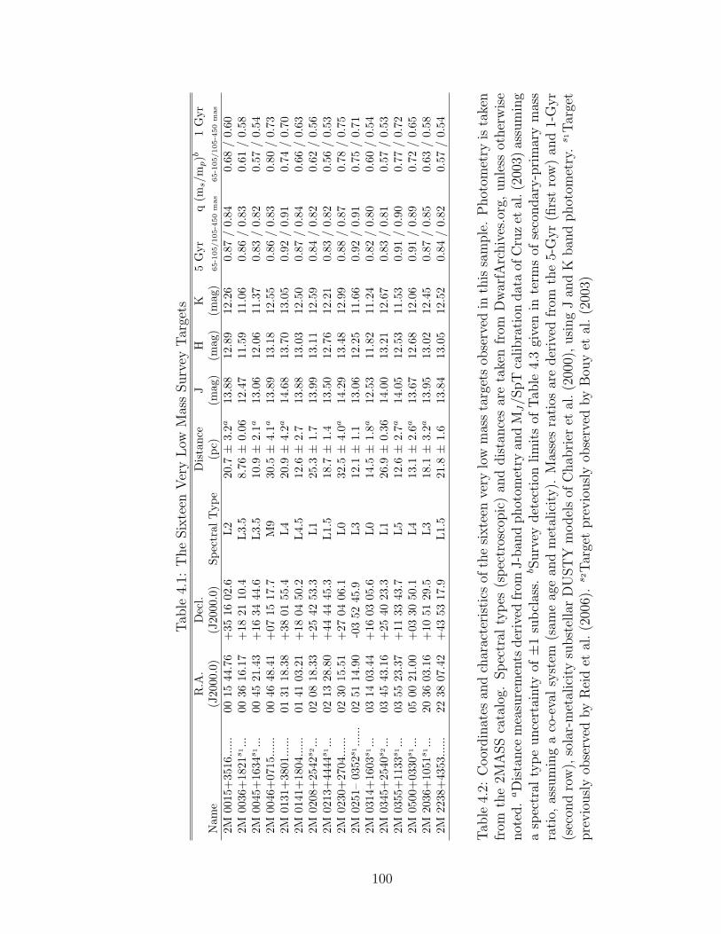
Tab
le4.
1:T
he
Six
teen
Ver
yL
owM
ass
Surv
eyT
arge
tsR
.A.
Dec
l.D
ista
nce
JH
K5
Gyr
q(m
s/m
p)b
1G
yrN
ame
(J20
00.0
)(J
2000
.0)
Spec
tral
Typ
e(p
c)(m
ag)
(mag
)(m
ag)
65-1
05/105-4
50
mas
65-1
05/105-4
50
mas
2M00
15+
3516
......
0015
44.7
6+
3516
02.6
L2
20.7±
3.2a
13.8
812
.89
12.2
60.
87/
0.84
0.68
/0.
602M
0036
+18
21s1...
0036
16.1
7+
1821
10.4
L3.
58.
76±
0.06
12.4
711
.59
11.0
60.
86/
0.83
0.61
/0.
582M
0045
+16
34s1...
0045
21.4
3+
1634
44.6
L3.
510
.9±
2.1a
13.0
612
.06
11.3
70.
83/
0.82
0.57
/0.
542M
0046
+07
15...
...00
4648
.41
+07
1517
.7M
930
.5±
4.1a
13.8
913
.18
12.5
50.
86/
0.83
0.80
/0.
732M
0131
+38
01...
...01
3118
.38
+38
0155
.4L
420
.9±
4.2a
14.6
813
.70
13.0
50.
92/
0.91
0.74
/0.
702M
0141
+18
04...
...01
4103
.21
+18
0450
.2L
4.5
12.6±
2.7
13.8
813
.03
12.5
00.
87/
0.84
0.66
/0.
632M
0208
+25
42s2...
0208
18.3
3+
2542
53.3
L1
25.3±
1.7
13.9
913
.11
12.5
90.
84/
0.82
0.62
/0.
562M
0213
+44
44s1...
0213
28.8
0+
4444
45.3
L1.
518
.7±
1.4
13.5
012
.76
12.2
10.
83/
0.82
0.56
/0.
532M
0230
+27
04...
...02
3015
.51
+27
0406
.1L
032
.5±
4.0a
14.2
913
.48
12.9
90.
88/
0.87
0.78
/0.
752M
0251
–03
52s1...
...02
5114
.90
-03
5245
.9L
312
.1±
1.1
13.0
612
.25
11.6
60.
92/
0.91
0.75
/0.
712M
0314
+16
03s1...
0314
03.4
4+
1603
05.6
L0
14.5±
1.8a
12.5
311
.82
11.2
40.
82/
0.80
0.60
/0.
542M
0345
+25
40s2...
0345
43.1
6+
2540
23.3
L1
26.9±
0.36
14.0
013
.21
12.6
70.
83/
0.81
0.57
/0.
532M
0355
+11
33s1...
0355
23.3
7+
1133
43.7
L5
12.6±
2.7a
14.0
512
.53
11.5
30.
91/
0.90
0.77
/0.
722M
0500
+03
30s1...
0500
21.0
0+
0330
50.1
L4
13.1±
2.6a
13.6
712
.68
12.0
60.
91/
0.89
0.72
/0.
652M
2036
+10
51s1...
2036
03.1
6+
1051
29.5
L3
18.1±
3.2a
13.9
513
.02
12.4
50.
87/
0.85
0.63
/0.
582M
2238
+43
53...
...22
3807
.42
+43
5317
.9L
1.5
21.8±
1.6
13.8
413
.05
12.5
20.
84/
0.82
0.57
/0.
54
Tab
le4.
2:C
oor
din
ates
and
char
acte
rist
ics
ofth
esi
xte
enve
rylo
wm
ass
targ
ets
obse
rved
inth
issa
mple
.P
hot
omet
ryis
take
nfr
omth
e2M
ASS
cata
log.
Sp
ectr
alty
pes
(sp
ectr
osco
pic
)an
ddis
tance
sar
eta
ken
from
Dw
arfA
rchiv
es.o
rg,
unle
ssot
her
wis
enot
ed.aD
ista
nce
mea
sure
men
tsder
ived
from
J-b
and
phot
omet
ryan
dMJ/S
pT
calibra
tion
dat
aof
Cru
zet
al.(2
003)
assu
min
ga
spec
tral
typ
eunce
rtai
nty
of±
1su
bcl
ass.
bSurv
eydet
ecti
onlim
its
ofT
able
4.3
give
nin
term
sof
seco
ndar
y-p
rim
ary
mas
sra
tio,
assu
min
ga
co-e
val
syst
em(s
ame
age
and
met
alic
ity).
Mas
ses
rati
osar
eder
ived
from
the
5-G
yr
(firs
tro
w)
and
1-G
yr
(sec
ond
row
),so
lar-
met
alic
ity
subst
ella
rD
UST
Ym
odel
sof
Chab
rier
etal
.(2
000)
,usi
ng
Jan
dK
ban
dphot
omet
ry.s 1
Tar
get
pre
vio
usl
yob
serv
edby
Rei
det
al.
(200
6).s 2
Tar
get
pre
vio
usl
yob
serv
edby
Bou
yet
al.
(200
3)
100

Tab
le4.
3:Surv
eyC
ontr
ast
Lim
its
(∆K
)at
99.5
%C
onfiden
ce
∆Ka
Pri
mar
y65
.085
.010
5.0
125.
014
5.0
165.
018
5.0
225.
026
5.0
305.
034
5.0
385.
042
5.0
2M00
15+
3516
0.92
1.52
1.73
1.88
2.07
2.25
2.27
2.18
2.03
1.82
2.06
2.06
1.79
2M00
36+
1821
1.77
2.30
2.52
2.57
2.63
2.74
2.77
2.79
2.71
2.70
2.62
2.67
2.56
2M00
45+
1634
2.06
2.61
2.82
2.87
2.90
2.96
3.01
3.02
2.94
2.93
2.80
2.86
2.84
2M00
46+
0715
0.62
1.01
1.16
1.29
1.48
1.58
1.66
1.60
1.38
1.27
1.28
1.35
1.22
2M01
31+
3801
0.74
1.26
1.30
1.30
1.35
1.47
1.52
1.55
1.45
1.28
1.25
1.41
1.25
2M01
41+
1804
1.52
2.13
2.37
2.51
2.55
2.61
2.65
2.59
2.58
2.58
2.41
2.51
2.42
2M02
08+
2542
1.29
1.93
2.16
2.28
2.35
2.48
2.52
2.47
2.34
2.28
2.29
2.32
2.25
2M02
13+
4444
1.84
2.40
2.59
2.64
2.72
2.77
2.79
2.81
2.76
2.73
2.59
2.69
2.58
2M02
30+
2704
0.72
1.11
1.20
1.18
1.23
1.27
1.30
1.32
1.27
1.09
1.03
1.26
1.08
2M02
51-0
352
0.69
1.07
1.24
1.26
1.32
1.39
1.48
1.38
1.36
1.28
1.24
1.37
1.34
2M03
14+
1603
1.52
2.08
2.32
2.47
2.54
2.60
2.65
2.61
2.54
2.50
2.51
2.52
2.39
2M03
45+
2540
1.75
2.28
2.51
2.56
2.61
2.70
2.76
2.75
2.61
2.57
2.55
2.58
2.51
2M03
55+
1133
0.69
1.15
1.21
1.05
1.04
1.22
1.27
1.25
1.29
1.32
1.24
1.27
1.12
2M05
00+
0330
0.79
1.35
1.53
1.64
1.81
1.97
2.02
1.99
1.80
1.57
1.80
1.83
1.57
2M20
36+
1051
1.30
1.90
2.10
2.26
2.31
2.41
2.50
2.40
2.31
2.24
2.26
2.30
2.18
2M22
38+
4353
1.77
2.29
2.51
2.53
2.57
2.63
2.71
2.69
2.57
2.54
2.52
2.56
2.50
Tab
le4.
4:D
etec
tion
contr
ast
lim
its
arou
nd
pri
mar
ies:
aP
rim
ary-S
econ
dar
yse
par
atio
ns
are
give
nin
unit
sof
mas
,an
dth
eco
rres
pon
din
gdet
ecti
onlim
its
are
in∆
Km
agnit
udes
.
101

Tab
le4.
5:M
odel
Fit
sto
Can
did
ate
Bin
arie
s
J.
Dat
eS
epar
atio
nA
z.A
ng.
Con
tras
tB
ayes
Sep
arat
ion
Pri
mar
y(+
2450
00)
(mas
)(d
eg)
Rat
ioF
acto
rC
onf.
(AU
)
2M00
36+
1821
4731
89.5±
11.4
114.
1±
5.5
13.1
4±
3.14
7.9
96%
0.78±
0.10
2M03
45+
2540
4731
217.
4±
9.1
258.
8±
2.8
26.4
4±
4.22
7.6
98%
5.85±
0.26
352.
7±
10.5
87.6±
2.0
30.7
9±
9.08
96%
9.49±
0.31
2M22
38+
4353
4732
128.
2±
10.3
209.
9±
5.3
17.7
6±
4.25
7.1
97%
2.79±
0.30
228.
5±
9.1
251.
8±
3.5
23.7
9±
5.92
95%
4.98±
0.42
395.
5±
9.7
19.5±
1.2
17.6
3±
4.22
97%
8.62±
0.66
2M03
55+
1133
4757
82.5±
13.0
276.
2±
4.1
2.10±
0.40
6.3
90%
1.03±
0.27
102
4.4 Sixteen Brown Dwarf Targets - Four Candidate Bina-
ries
Aperture masking is most sensitive to companions between λ/2D and 4λ/D, cor-
responding to angular separations of 60-450 mas in Ks at Palomar and physical
projected separations ranging from 0.6-10 AU for the targets in our survey.
Our achieved detection limits for all sixteen targets are summarized in Table
4.3. Our limits remain relatively flat at separations beyond λ/D, plateauing near
∆K∼2.3 for more than half our targets, and decline to roughly 1.4 magnitude
shortward of λ/D (See figure 4.5).
We infer the (companion) stellar properties and mass ratios to the correspond-
ing magnitude limits using the DUSTY models for target ages of 5 Gyr and 1 Gyr
(Table 4.1). At the formal diffraction limit (about 110 mas in Ks), companions
with mass ratios of .83 for 5 Gyr systems and .55 for 1 Gyr systems would be
resolved for 50% of our targets at a 99.5% confidence of detection (Fig. 4.6).
Our survey found four candidate binary systems with detections at 90-99% con-
fidence and Bayes’ Factors favoring the binary model (Table 4.5). We summarize
and discuss these detections below.
For some targets in our survey, closure phase measurements constructed from
the longest baselines had too much noise to extract a useable signal. The resulting
drop in uv-coverage can give rise to aliasing of the model fits: i.e., multiple binary
configurations fit the data equally well. When possible, we used previous observa-
tions of the target to rule out certain aliased fits; when not possible, all model fits
are listed.
103
2M 0036+1821: A companion at separation 89.5 mas and 13.1:1 contrast
was detected with 96% confidence and a Bayes’ Factor of 7.8:1. The data also fits
an alternative (alias) binary configuration (ρ ∼ 243 mas and 25:1 contrast) with
96% confidence that we rule out by a previous observations. Reid et al. (2006)
observed this target in November 2005 with the NICMOS imager on the Hubble
Space Telescope in the F170M and F110W bands. At or near this separation, this
alternative configuration would have likely been detectable in the F110W bands.
2M 0355+1133: A companion at separation 82.5 mas and 2.1:1 contrast was
detected with 90% confidence and a Bayes’ Factor of 6.3:1. Reid et al. (2006) also
observed this target in the F110W band and found no companion. As a proxy for
the F110W bandpass, we estimate a J band contrast of 2.5:1 using the J-K color-
magnitude relations of Dahn et al. (2002). Their program achieved a contrast limit
of 2.5:1 beyond approximately 100 mas in F110W, suggesting that this candidate
binary sat at the edge of their detection limits.
2M 2238+4353: Thirty-five percent of the closure phase triangles showed
very high noise and were removed from analysis. As a result, aliasing of the signal
was particularly problematic. Three distinct binary configurations were detected
at 95-97% confidence. These range in separations between 100 and 400 mas and
contrasts between 17:1 and 28:1.
2M 0345+2540: Like 2M 2238+4353, a large percentage of the closure phases
were removed from analysis. Two distinct configurations, both with contrasts
∼28:1 (∆K ∼ 3.5) were determined with high confidence. Bouy et al. (2003)
observed this target with the Wide Field Planetary Camera 2 (WFPC2) on the
Hubble Space Telescope in March 2001, but we estimate these companions to
be below their detection limits. Their survey reached background limitations at
104
contrasts between ∆M ∼3-5 in the F814W band. Using the I band as a proxy for
F814W, we estimate the companion of 2M 0345+2540 to have a contrast of ∆I &5
and to have been undetectable in the Bouy survey.
2M0213+4444: We observed target 2M0213+4444 three times over two
nights in September 2008 (two sets in Ks, one in H) and once one month later
(in Ks). Two data sets from September were of poor quality and were not used
for analysis. The remaining set from September found one binary fit (ρ ∼ 81 mas,
θ ∼ 290◦, 5.2:1 contrast in Ks) at 89% confidence. The target was observed again
in Ks in October under poor seeing and much of the data was unusable. This data
set could not be fit well by the September results, and implied a different config-
uration with 90% confidence (ρ ∼ 234 mas, θ ∼ 135◦, 11:1 contrast in Ks). Given
the low confidences of fits and the unreproducibility of these results, we conclude
that this target is unlikely to be binary.
4.5 Discussion: Aperture Masking of Faint Targets
The use of non-redundant masking removes many types of spatial perturbations to
the incoming wavefront. During high signal to noise observations, when read and
background noise are minimal, the largest contributor to measurement noise is the
temporal and spatial atmospheric fluctuations of the wavefront, even after adaptive
optics correction. Short exposure times, roughly less than the coherence time of
atmosphere, freezes the tip-tilt and low-order perturbations to the wavefront, which
can be removed by combining fringe phases into closure phases. This advantage
is lost when exposures extend over multiple coherence times. For this reason,
aperture masking flourishes with short exposures.
105
Behind laser guide star adaptive optics systems, although the structure of the
corrected wavefront may be different, the functionality of aperture masking is the
same. However, targets requiring laser guide star AO tend to be fainter, and thus
require either longer exposure times (permitting sufficient correction) or techniques
for dealing directly with noise from read outs and background flux.
This survey opted for maintaining short exposure times. The signal to noise of
fringe amplitudes decline rapidly for longer baselines, as the transmission function
for these baselines is lower and turbulence variations are larger. Just as, for in-
stance, Stehl ratio depends on the variance of the incoming wavefront, so does the
fringe amplitude, also dropping as exp(−σ2baseline). For faint targets, long baselines
fringes often linger undetectable below the background and read noise, making
difficult measurements of long baseline phases.
The capture of a large number of short exposure images allows us to select out
the best fringe measurements, during the serenditous moments of very good correc-
tion or still atmospheres, and discard those dwarfed by read noise. This technique,
analogous to lucky imaging, effectively selects high signal to noise measurements of
closure phase. In most cases, these lucky closure phases were sufficient to obtain
measurements of the target closure phase, even at long baselines. We contrast this
method to two measurements of targets observed with long (1 minute) exposures.
These exposures did often have long baseline fringes detectable at or just above
background. But this method resulted in poor measurements of the target closure
phase, even at shorter baselines. The multiple-coherence time exposures means
that low order perturbations are not effectively removed by closure phases, result-
ing in large phase errors, and the fewer overall number of data points removes the
statistical advantage. The measured closure phase is not a good measurement of
106
the true target phase.
Long exposures, with adequate correction, do allow longer baseline fringes to
grow in amplitude above the read noise or background limit. Exposures for aper-
ture masking should be limited to the effective coherence time of the adaptive
optics system – the interval over which the phase variance of the longest baselines
reaches about one radian.
The quality of measurements from both sets of exposure data suggests a slight
modification of technique for the next application of aperture masking with laser
guide star adaptive optics. The higher noise content of the one-minute exposures
suggests that these exposures are too long for the level of correction obtained in
this survey. The short exposure method fared much better, but a large percentage
of images failed to observe fringe amplitudes above read noise. This suggests that
slightly longer exposures would have benefited the observations. It is worthwhile
to note that the low transmission of the long baselines, even at Strehl ratios of
15% typically reached in this survey, indicates that direct imaging would not have
been able to obtain λ/D resolution.
4.6 Conclusion
We present the results of a close companion search around nearby L dwarfs using
aperture masking interferometry and Palomar laser guide star adaptive optics. The
combination of these techniques yielded typical detection limits of ∆Ks = 1.5-2.5
between 1-4λ/D and limits of ∆Ks = 1.0-1.7 at 0.6 λ/D. Our survey revealed
four candidate binaries with moderate to high confidence (90-99%) and favorable
Bayes’ Factors.
107
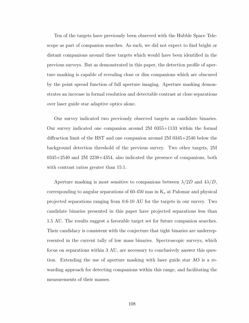
Ten of the targets have previously been observed with the Hubble Space Tele-
scope as part of companion searches. As such, we did not expect to find bright or
distant companions around these targets which would have been identified in the
previous surveys. But as demonstrated in this paper, the detection profile of aper-
ture masking is capable of revealing close or dim companions which are obscured
by the point spread function of full aperture imaging. Aperture masking demon-
strates an increase in formal resolution and detectable contrast at close separations
over laser guide star adaptive optics alone.
Our survey indicated two previously observed targets as candidate binaries.
Our survey indicated one companion around 2M 0355+1133 within the formal
diffraction limit of the HST and one companion around 2M 0345+2540 below the
background detection threshold of the previous survey. Two other targets, 2M
0345+2540 and 2M 2238+4354, also indicated the presence of companions, both
with contrast ratios greater than 15:1.
Aperture masking is most sensitive to companions between λ/2D and 4λ/D,
corresponding to angular separations of 60-450 mas in Ks at Palomar and physical
projected separations ranging from 0.6-10 AU for the targets in our survey. Two
candidate binaries presented in this paper have projected separations less than
1.5 AU. The results suggest a favorable target set for future companion searches.
Their candidacy is consistent with the conjecture that tight binaries are underrep-
resented in the current tally of low mass binaries. Spectroscopic surveys, which
focus on separations within 3 AU, are necessary to conclusively answer this ques-
tion. Extending the use of aperture masking with laser guide star AO is a re-
warding approach for detecting companions within this range, and facilitating the
measurements of their masses.
108
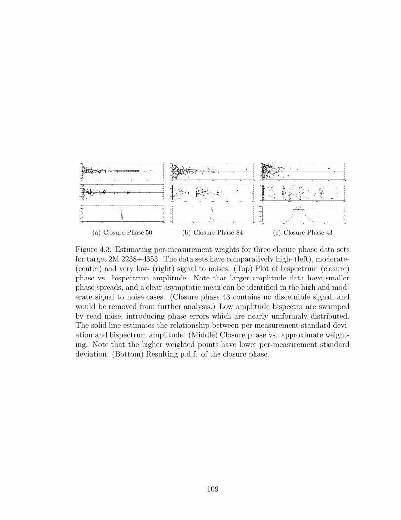
(a) Closure Phase 50 (b) Closure Phase 84 (c) Closure Phase 43
Figure 4.3: Estimating per-measurement weights for three closure phase data setsfor target 2M 2238+4353. The data sets have comparatively high- (left), moderate-(center) and very low- (right) signal to noises. (Top) Plot of bispectrum (closure)phase vs. bispectrum amplitude. Note that larger amplitude data have smallerphase spreads, and a clear asymptotic mean can be identified in the high and mod-erate signal to noise cases. (Closure phase 43 contains no discernible signal, andwould be removed from further analysis.) Low amplitude bispectra are swampedby read noise, introducing phase errors which are nearly uniformaly distributed.The solid line estimates the relationship between per-measurement standard devi-ation and bispectrum amplitude. (Middle) Closure phase vs. approximate weight-ing. Note that the higher weighted points have lower per-measurement standarddeviation. (Bottom) Resulting p.d.f. of the closure phase.
109
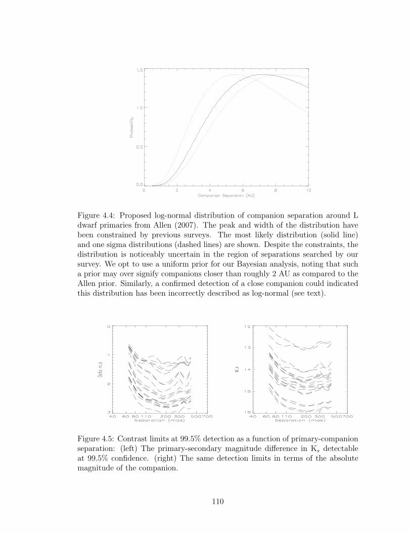
Figure 4.4: Proposed log-normal distribution of companion separation around Ldwarf primaries from Allen (2007). The peak and width of the distribution havebeen constrained by previous surveys. The most likely distribution (solid line)and one sigma distributions (dashed lines) are shown. Despite the constraints, thedistribution is noticeably uncertain in the region of separations searched by oursurvey. We opt to use a uniform prior for our Bayesian analysis, noting that sucha prior may over signify companions closer than roughly 2 AU as compared to theAllen prior. Similarly, a confirmed detection of a close companion could indicatedthis distribution has been incorrectly described as log-normal (see text).
Figure 4.5: Contrast limits at 99.5% detection as a function of primary-companionseparation: (left) The primary-secondary magnitude difference in Ks detectableat 99.5% confidence. (right) The same detection limits in terms of the absolutemagnitude of the companion.
110
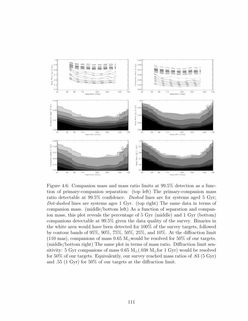
Figure 4.6: Companion mass and mass ratio limits at 99.5% detection as a func-tion of primary-companion separation: (top left) The primary-companion massratio detectable at 99.5% confidence. Dashed lines are for systems aged 5 Gyr;Dot-dashed lines are systems ages 1 Gyr. (top right) The same data in terms ofcompanion mass. (middle/bottom left) As a function of separation and compan-ion mass, this plot reveals the percentage of 5 Gyr (middle) and 1 Gyr (bottom)companions detectable at 99.5% given the data quality of the survey. Binaries inthe white area would have been detected for 100% of the survey targets, followedby contour bands of 95%, 90%, 75%, 50%, 25%, and 10%. At the diffraction limit(110 mas), companions of mass 0.65 M�would be resolved for 50% of our targets.(middle/bottom right) The same plot in terms of mass ratio. Diffraction limit sen-sitivity: 5 Gyr companions of mass 0.65 M�(.038 M�for 1 Gyr) would be resolvedfor 50% of our targets. Equivalently, our survey reached mass ratios of .83 (5 Gyr)and .55 (1 Gyr) for 50% of our targets at the diffraction limit.
111
CHAPTER 5
THE USE OF SPATIAL FILTERING WITH APERTURE MASKING
INTERFEROMETRY AND ADAPTIVE OPTICS1
5.1 Abstract
Non-redundant aperture masking interferometry with adaptive optics is a powerful
technique for high contrast at the diffraction limit with high-precision astrometry
and photometry. A limitation to the achievable contrast can be attributed to
spatial fluctuations of the wavefront - those within a sub-aperture and across sub-
apertures - and temporal fluctuations within a single-exposure. Spatial filtering
addresses spatial fluctuations within a sub-aperture. An optimized pinhole in the
focal place preceding the aperture mask is one approach for reducing the variation
of the wavefront within a sub-aperture. Similarly, a weak spatial filtering effect is
shown to be provided by post-processing the images with an apodized window func-
tion, typically used to minimize detector read noise and contamination from wide-
separated sources. We explore the effects of spatial filtering through calculation,
simulation, and observational tests conducted with a pinhole and aperture mask in
the PHARO instrument at the Hale 200” Telescope at Palomar Observatory. We
find that a pinhole decreases stochastic closure phase errors and calibration errors,
but that tight restrictions are placed onto the alignment of binary targets within
the pinhole. We propose an observation strategy to relax these restrictions. If im-
plemented the pinhole could potentially yield an increase in achievable contrast by
up to 10-25% in H and Ks bands, and more at very high Strehl (&80%). We also
conclude that correcting low-order wavefront modes within the sub-apertures will
1This work has been under review for publication by the The Astrophysical Journal as ofAugust 1, 2011.
112
be key for reaching high contrasts with extreme-AO systems such as the Gemini
Planet Imager and PALM3K to search for planets.
5.2 Introduction
Current planetary searches using a coronagraph (e.g., Hinkley et al. (2011)), excel
at obtaining very high contrast (105:1) but are unable to probe at close separations
(.300-500 mas) where the field of view is blocked by the occulting spot. This sep-
aration rules out the observation at physical separations . 10 AU for many host
stars. The detection of planetary companions with techniques providing both high-
contrast and high-resolution will play a key role in identifying the full distribution
of Jupiter-class planets and for investigating the mechanisms of planetary forma-
tion (Kraus et al., 2009), migration, and stability (Veras et al. (2009); Raymond
et al. (2009) and e.g. HR 8799, Fabrycky & Murray-Clay (2010)).
Non-Redundant Aperture Masking Interferometry (NRM or aperture masking),
in conjunction with adaptive optics (AO) is well established for yielding much more
precise astrometry and photometry than adaptive optics alone at close separations
(e.g., Kraus et al. (2008, 2011)) and for the detection of high contrast companions
(Lloyd et al., 2006). The application of aperture masking with AO on 5-10 meter
class telescopes achieves contrasts of 102-103:1 at and outward of λ/D and nicely
complements companion searches with a coronagraph. The increased contrast
and resolution of NRM has been used with great effect for stellar multiplicity
studies (Kraus et al., 2008, 2011), the detection of short period brown dwarfs for
dynamical mass measurements (Lloyd et al., 2006; Bernat et al., 2010), and a
high-contrast search for inner planetary companions to HR 8799 (Hinkley et al.,
113
2011). With the Gemini Planet Imager (Macintosh et al., 2008) and Project 1640
IFS (Hinkley et al., 2009) equipped with non-redundant masks, aperture masking
interferometry from the ground will play a key role in the detection of exoplanets
at close separations.
NRM observations use a mask to transform the full telescope aperture into a
sparsely populated set of sub-apertures, constructed so that no two pairs of sub-
apertures share the same baseline direction and length (i.e., are non-redundant).
The strength of this technique draws on its measurement of the closure phase
quantity (e.g., Jennison (1958); Readhead et al. (1988); Cornwell (1989)), an ob-
servable which naturally mitigates the effect of wavefront errors on scales larger
than a sub-aperture. These same wavefront errors produce the speckles of direct
imaging, which dominate the image noise by orders of magnitude whether arising
from atmospheric variation (Racine et al., 1999) or quasi-static instrumental effects
(Hinkley et al., 2007). Their mitigation by closure phases enables higher contrast
despite the blocking of 90-95% of the flux by the aperture mask.
The achievable contrast of the technique is limited by its own calibration chal-
lenges, one of which arises from quasi-static spatial variation of the wavefront
within the sub-aperture. Such wavefront errors erode the effectiveness of using
closure phases (resulting in redundancy noise in the language of Readhead et al.
(1988) and others). Similarly, decreasing the wavefront variation within the sub-
aperture can increase the contrast of NRM observations further.
Optical and infrared long-baseline interferometers have implemented single-
mode fibers and pinholes which spatially filter (i.e., smooth) aperture wavefront
errors to improve measurements of complex visibility (Shaklan & Roddier, 1987;
du Foresto et al., 1997). Poyneer & Macintosh (2004) have studied the use of a
114
pinhole to develop an AO wavefront sensor which more accurately measures of
the wavefront above a sub-aperture. Likewise, spatially filtering the wavefront
errors with a pinhole placed in the image (focal) plane before the aperture mask
may provide a means for substantially increasing the achievable contrast of NRM
observations.
This paper provides a comprehensive analysis of NRM with pinhole spatial
filtering. To establish its theoretical foundation, we present an analytic description
of the combined technique (Section 2). Using an accurate simulation of an aperture
masking equipped telescope, we derive the optimal pinhole size and estimate its
expected performance, limitations, and restrictions. We also derive several results
applicable to general aperture masking observations. (Sections 3 and 4). We have
also installed a pinhole in the PHARO instrument of the Hale 200” Telescope at
Palomar Observatory. To study how spatial filtering improves the sensitivity of
NRM observations and influences the astrometric and photometric characterization
of discovered binary systems, we observed twenty-six single stars and four known
binaries with and without the pinhole (Section 5). This paper further develops
the understanding of NRM as a technique for detecting high-contrast companions
and provides several new findings to guide the design of NRM experiments for
next generation adaptive optics systems and instruments dedicated to exoplanet
detection.
115
5.3 Aperture Masking with Spatial Filtering
5.3.1 Aperture Masking: Current Technique
An aperture mask is positioned in the pupil plane behind the adaptive optics sys-
tem and transforms the full aperture into a sparsely populated set of sub-apertures
(Fig. 5.1(a)). The resulting image of the target is a set of over-lapping fringes
called the interferogram. The amplitude and phase of each fringe corresponds to
the measurement of one particular component of the complex visibility with spatial
frequency ~b/λ, where ~b is the baseline vector and λ is the observing wavelength.
Multiplying the complex visibility of specific baseline triplets formed by three sub-
apertures creates bispectra (Lohmann et al., 1983), the argument of which is the
closure phase (Jennison, 1958; Cornwell, 1989). Closure phases are robust against
pupil-plane phase errors, which are a source of direct imaging PSF calibration
errors and speckle noise, and provide the mechanism for obtaining more precise
astrometry and photometry with the aperture masking technique.
Typical observations (including those in this paper) are conducted by taking
one or more sets of target images interspersed with sets of one or more calibra-
tors (unresolved stars near in the sky and of similar magnitude and color.) After
the basic processing the raw images (see, for example, Lloyd et al. (2006); Mar-
tinache et al. (2007); Bernat et al. (2010)), the phase and log-amplitude of each
fringe is extracted from the images and used to construct bispectra and closure
phases. Mean values are obtained by averaging the quantities over a single set,
and error estimates are derived from the scatter. Multiple sets are combined by
weighted average. Calibration is performed by subtracting the closure phase and
log-amplitude of the reference stars. Amplitudes are generally not used in com-
116
panion searches because calibration is subject to stable atmospheric seeing and
often is measurable to only 10-50% (Tuthill et al., 2006). A binary model is fit to
the closure phase data to minimize χ2; a positive detection results in measurement
of the binary parameters (separation, orientation, and wavelength-dependent con-
trast ratio). Errors in binary parameters are often taken from the curvature of the
χ2 space at minimum. Many examples of this implementation for the detection of
stellar companions can be found in the literature (Kraus et al., 2008; Bernat et al.,
2010; Kraus et al., 2011).
For targets in which the adaptive optics system provides stable and mostly
coherent (σ2rms . 0.1 rad2) correction of the wavefront on sub-aperture scales,
this observing mode typically measured closure phases with an error scatter of 1-2
degrees in H band (1.6µm) after a few minutes on a bright target, equivalent to
a contrast of detection of about 100-200:1 at λ/D. This technique is calibration
limited by a systematic closure phase component of one to several degrees which
likely arises from quasi-static instrumental wavefront errors. Additional calibrators
usually decrease, but do not fully eliminate, this component. To account for this,
an addition error term is added in quadrature to the closure phase errors until the
best fitting model yields a χ2 of unity.
5.3.2 Aperture Masking: Why Spatial Filter? Calibration
Errors.
A critical requirement of the aperture masking design is that each pair of sub-
aperture creates a unique interferometric baseline. The lack of baseline redundancy
ensures that any spatial frequency measured can be traced back to the interfer-
117
ence of a unique pair of sub-apertures (Haniff et al., 1987; Roddier, 1986). Closure
phases constructed by non-redundant baselines will be less affected by pupil-plane
phase which would otherwise distort measurements of the spatial frequency phase.
When two or more baselines contribute to the same spatial frequency, the power
adds partially incoherently depending on the phase difference of each contribut-
ing baselines (e.g., Figure 5.1(b)). A random component will be introduced into
the resulting spatial frequency phase which cannot be removed by closure phases
(yielding a so-called non-zero closure phase). This component, termed redundancy
noise, is largest when the redundant baselines are incoherent and zero when the
they are coherent. Readhead et al. (1988) provides an extensive treatment of
redundancy noise for seeing-limited imaging.
The mask cannot be entirely non-redundant. The finite sub-aperture size means
that baselines are redundant at least within a sub-aperture (Figure 5.1(c)). With
sub-aperture scale correction provided by the AO system, this sub-aperture redun-
dancy noise is largely removed (Tuthill et al., 2006), as compared to the uncorrected
case, but still gives rise to closure phase measurement errors due to the remain-
ing spatial incoherence within the sub-aperture. In completely analogous fashion,
temporal variations to the baseline phase during a single exposure create temporal
redundancy which also give rise to closure phases errors (again, see Readhead et al.
(1988)).
It may be illuminating to contrast the uncorrected and corrected cases. With
uncorrected observing, redundancy restricts sub-aperture sizes to smaller than the
characteristic size of atmospheric turbulence and exposure times shorter than the
atmospheric coherence time. Adaptive optics removes both constraints since good
correction supplies a stable, mostly coherent wavefront across the full aperture.
118
Current NRM masks are designed with sub-apertures on the order of the AO
actuator spacing; this need not be the case and will likely not be so in upcom-
ing extreme-AO aperture masking experiments. Atmospheric and adaptive optics
residuals decorrelate on timescales much shorter than the exposure length and
thus likely only contribute to the stochastic variation of closure phases from one
image to the next. Changes in seeing between target and calibrator observations
change the magnitude of the stochastic variability of closure phases (the signal
to noise of the measurement), but do not introduce calibration offsets (Roddier,
1986), and can thus be minimized by additional exposures. This is precisely why
closure phases provide a robust measurable unlike visibility amplitudes, which are
poorly calibrated if seeing changes (Tuthill et al., 2006).
Quasi-static instrumental wavefront errors contribute to all spatial scales and
vary on timescales of tens of minutes (e.g., Bloemhof et al. (2001); Hinkley et al.
(2007)), or with movement of the telescope (Marois et al., 2005). As long as these
errors remain static over a single exposure, large-scale wavefront changes (those
larger than a sub-aperture) are removed by closure phases. One of the great
advantages of using non-redundant masking to mitigate the quasi-static imaging
problem is that closure phases require only a single image (they ’self-calibrate’,
Cornwell (1989)). Instrumental errors change between observations of the target
and calibrator, but only those smaller scale than a sub-aperture contribute to
aperture masking calibration errors.
We propose that spatial filtering the wavefront before its propagation through
the aperture mask can be used to reduce the inhomogeneity of the wavefront
phase within the sub-aperture and, by virtue of being more coherent, reduce sub-
aperture redundancy noise. Figure 5.2 illustrates the effect of an optimized pinhole
119
spatial filter (discussed in the next subsection) to smooth the phase of a simulated
adaptive optics corrected wavefront (Strehl ratio ∼ 50% in Ks). The portion of
the wavefront sampled by each sub-aperture is much more uniform after spatial
filtering.
We anticipate that spatial filtering can lead to several measurable improve-
ments of the closure phases, including decreases in systematic calibration error
and stochastic variation from one image to the next. Measured visibility ampli-
tudes, by virtue of their dependence on sub-aperture inhomogeneity, can show less
degradation and be more robust to changes in seeing.
5.3.3 Pinhole Filtering
One possible implementation of the pinhole spatial filter, reminiscent of the four
planes of a coronagraph (see Ferrari (2007) for a review), is shown in Figure 5.3.
The pinhole, positioned at the center of the field and in what is usually referred to
as the coronagraphic plane, blocks light beyond its inner transmission region. This
acts to spatially filter the wavefront before entering the non-redundant aperture
mask, located in a re-imaged pupil plane. (The mask location is equivalent to the
Lyot-plane of coronagraphy).
The transmission profile of the pinhole is a top-hat function, with diameter
dspf which will be expressed for convenience in units of λ/D, with D the diameter
of the telescope. At the location of the aperture mask, this is equivalent to the
wavefront convolved by a Jinc function (c.f. Footnote 1) of characteristic diameter
λ/dspf .
0The Jinc function is defined as Jinc(x) ≡ J1(x)x . It is the two-dimensional Fourier Transform
of a circular aperture, and is related to the Airy function by Airy(x) = 4 Jinc(x)2.
120

Efficient spatial filtering aims to make the wavefront uniform within one sub-
aperture of the non-redundant mask, and so one wants the characteristic diameter
to be matched to the diameter of a sub-aperture, suggesting
dspf ≈D
dsub(in units of λ/D). (5.1)
A larger pinhole decreases the impact of the spatial filtering; a smaller pinhole
restricts the field of view and begins to impinge on the signal we wish to measure.
This technique differs from the form of spatial filtering implemented in optical
and infrared long baseline interferometers, where the signal from each telescope is
injected into a single mode fiber or pinhole before beam combination and extraction
of the interferometric signals (du Foresto et al., 1997). The use of single mode
fibers on long baseline interferometers has shown increases in phase estimations by
a factor of two, or more in bad seeing, despite the loss of flux (Tatulli et al., 2010).
The implementation of this approach with non-redundant aperture masking would
require the injection of light from each sub-aperture into a single mode fiber or
pinhole before recording the interferogram. Given the simplification of the single
pinhole implementation, it offers, a priori, an appealing alternative (Keen et al.,
2001).
Aperture Masking Through a Pinhole
Given that the aperture mask is located in a pupil plane, the point spread function
(PSF) of masking interferometry is invariant to target position over a wide field
of view (several arc seconds). With the pinhole filter in place (in an image plane),
the PSF and system response varies with target position relative to the pinhole, a
121
smaller effective field of view.
Section 5.9 shows that the use of the pinhole filter alters the measured complex
visibility of a point source:
Vspf (~b) = T (~b)
∫d~θ Π[~θ/dspf ]× e2πi~θ·~b/D × PSF [θ − ~α], (5.2)
where ~α is the location of the point source on the sky (measured in angular units of
λ/D), and ~α = 0 corresponds to perfect alignment of the source in the pinhole. The
baseline being measured is ~b, corresponding to a spatial frequency ~u = ~b/λ. The
complex visibility is usually expressed as a function of the spatial frequency; here
we present it as a function of baseline and wavelength for clarity. The telescope
transfer function, T (~b), gives the spatial frequency response of the aperture or
aperture mask in terms of the baseline. It is defined explicitly in Section 5.9. The
top-hat function, Π[ |~θ|
dspf], is equal to one for |~θ|
dspf< 1
2and zero otherwise.
From three baselines vectors, ~b1, ~b2, and −~b1 −~b2, a closure phase is the argu-
ment the product of the complex visibilities:
φcp = arg[V (~b1)V (~b2)V (−~b1 −~b2)
](5.3)
The observed visibility amplitudes and closure phase change by an amount
which depends on the position of the target with respect to the pinhole (its align-
ment) and the point spread function. (e.g., Figure 5.4). The transmission of the
pinhole blocks high spatial frequency content of the wavefront, even in the absence
of wavefront errors. In this way, removal of the higher spatial frequencies can
alias into changes in lower, baseline frequencies, similar to the effect observed by
Poyneer & Macintosh (2004). Those on sub-aperture scales compete with closure
phase measurements.
122
As the point spread function varies, so too will the aliased phase errors. This
introduces a stochastic component to the closure phase errors which appears to
undercut the effectiveness of the pinhole. A portion of the phase errors will also
remain fixed and be strictly a function of the asymmetrical truncation of the target
and its mean point spread function. The latter we term misalignment error, to
distinguish it from other calibration components. Generally speaking, both will
increase as the target is positioned further from the pinhole center.
Qualitatively, we can illustrate that the asymmetrical truncation of the target
shifts the visibility and closure phase. Consider Figure 5.4c. The visibility phase
is influenced by the position of the target on the sky; the asymmetrical truncation
of the target shifts its center of light, and so too the visibility phase. While closure
phases are normally invariant to the position of the target normally, the pinhole
breaks this invariance. The overall isotropy of the point spread function and cir-
cular pinhole shape suggests that the misalignment error is symmetric about the
origin. That is, just as aligning the target at two diametrically opposed positions
will induce equal and opposite shifts in the center of light, the overall symmetry
suggests equal and opposite phase errors as well.
The aliased phase errors are small as long as the majority of the flux resides
within the pinhole and only competes with the closure phase measurements if the
power aliases back into sub-aperture scale wavefront deviations. For this reason
shorter wavelength observations will be preferentially advantaged with this ap-
proach. More generally this suggests, that to minimize aliasing, the pinhole could
be optimized to filter only frequencies that are not corrected by the AO system;
in that case the pinhole size would be matched the the AO actuator size instead
of the masking sub-aperture size.
123
Each target of a binary will be truncated differently. The misalignment error
can be calculated directly by replacing the single star point spread function in
Equation 5.2 or Figure 5.4 with the binary image. This will be approximately the
same as the error of each component individually. In other words, the misalignment
error of the primary added to the misalignment error of the secondary multiplied
by the secondary-primary contrast ratio. Assuming that the misalignment error
is point symmetric about the origin, aligning the binary center of light near the
pinhole center appears to be a viable strategy for minimizing the misalignment
error.
If the misalignment component is large enough as to become the limiting com-
ponent in closure phase noise, there are three approaches which can be employed
for removing the component from science data. Empirically, the component can be
calibrated by observing a single star aligned at the same location as the primary
under similar AO performance. In practice, this may be limited by the accuracy
with which one can repeatedly (visually) align a target within the pinhole, and the
component arising from the (unknown) companion remains. Computationally, if
the location of the primary is known along with an estimate of the point spread
function, then the misalignment component can be included in the mathematical
closure phase model which is fit to data. This approach requires a direct image
of the primary within the pinhole to determine its location and estimate its point
spread function. Both may detract from the overall efficiency of observing. Finally,
a third option is to take several sets of aperture masking data with the target (cen-
ter of light) at various alignments. Specifically, if diametrically opposed alignments
have misalignment errors opposite in sign, then the component could be averaged
out.
124
5.3.4 Post-Processing with a Window Function
In this course of our investigation of the pinhole filter, we also characterize the use
of a tapered window function on masking images to reduce the impact of various
noise sources and small-scale wavefront errors on closure phases. For example,
we use a super-Gaussian function, exp(−kx4), with our experiments for its flat-
top and quickly tapering Fourier Transform. For concreteness, we will use this
same function as an illustrative example here (Figure 5.5). The window function
is described by the size of its half width at half max measured in pixels on the
detector or in units of λ/D.
Multiplying the images by a window function that retains the intensity of
the interferogram core but tapers at its edges greatly reduces the contamination
of detector read noise and dark current, or scattered light from nearby targets
not of scientific interest. Per-pixel Gaussian-distributed read noise, when Fourier
Transformed, results in a per-baseline Gaussian-distributed uncertainty. The per-
baseline noise has a magnitude that is directly related to the total transmission
of the window function. Therefore, a tighter window function removes more read
noise.
However, complex visibilities are extracted from the Fourier Transform of the
image, so the application of a window function is identical to the convolution
of the complex visibilities with the Fourier Transform of the window function.
This mixes the complex visibilities of the baselines and, ultimately, restricts the
minimum window function size.
The aperture mask is designed to be non-redundant for baselines extending
between the centers of sub-apertures; the finite size of the sub-apertures give rise
125
to islands of transmitted power in the power spectrum, which we call splodges (see
Figure 5.5, Bottom Left). The splodges of a completely non-redundant mask do
not overlap, and hence the separation between neighboring splodge peaks is about
2 dsub. (In practice, some overlap at the splodge edges may be exchanged for
better coverage or larger sub-apertures.) Furthermore, neighboring splodges may
arise from completely separate pairs of sub-apertures (i.e., separate baselines), and
one would not assume any coherence between the baseline phases. For this reason,
window functions narrower than about λ/2dsub, or those without quickly tapered
Fourier Transforms, will mix the incoherent baselines of neighboring splodges and
rapidly increase the error of closure phases, similar to redundancy noise.
The optimally sized window function will balance the reduction of read noise
with the increase of redundancy noise.
Post processing with a window function also reduces the impact of small-scale
wavefront errors. This is most readily recognized by noting that the outer rings
of the point spread function encapsulate the high spatial frequency content of the
wavefront; removing this flux also removes the high spatial frequency content of
the wavefront.
5.4 Simulated Observations
We have developed an accurate simulation of the Palomar aperture masking in-
terferometry experiment in order to explore the effect of spatial filtering on wide
band data and to optimize the pinhole for implementation on the telescope.
The Palomar 9-hole aperture mask has been described previously in Lloyd
126

et al. (2006) and is shown in Figure 5.1(a). Placed in the pupil plane, the mask
has baselines ranging from 0.71m to 3.94m and sub-apertures that are 0.42m in
diameter.
As discussed in Pravdo et al. (2006) and Bernat et al. (2010), aperture masking
and the implementation of closure phases works most effectively using the short
exposure times, when large scale wavefront errors (be they atmospheric or instru-
mental) can be regarded as approximately static. The typical aperture masking
operation at Palomar uses exposure lengths of 431 ms. Over this time scale, the
evolution of the atmosphere produces a highly dynamic wavefront on sub-aperture
scales.
5.4.1 Characterization and Simulation of Palomar’s Atmo-
sphere
Studies by Ziad et al. (2004) and Linfield et al. (2001) conducted with the Palo-
mar Testbed Interferometer (PTI) and Hale 200” Telescope confirm that the at-
mospheric turbulence power spectrum is approximately Kolmogorov with an outer
scale most often within the range 10 - 50 meters. The median-seeing Fried param-
eter (r0) has been measured to be 9.0 cm at 550 nm, dropping to 3.8 cm during
bad, but regularly observed seeing (Dekany et al., 2007).
Advection (wind) speeds drive the evolution of atmospheric structure within
the sub-aperture on intervals between 0.1 and 1.0 seconds. Using measurements
of the Palomar atmospheric temporal structure function over four nights, Linfield
et al. (2001) derive wind speeds typically less than 4 m/s. For shorter time scales,
the temporal structure function decays exponentially. The characteristic decay
127

time, which scales with λ6/5, has been measured in two surveys to vary between
15-80 ms (Ziad et al., 2004) and 60-150 msec (Linfield et al., 2001) in Ks.
Our simulations assume an outer scale of 50 meters and Fried parameter value
9.0 cm, which corresponds to 48 cm in Ks and 32 cm in H. We use wind speeds of
5 m/s and temporal decay time of 60 ms.
5.4.2 Numerical Simulation
We generate time-evolved Kolmogorov phase screens following the procedures of
Lane et al. (1992) and Glindemann et al. (1993). These phase screens are char-
acterized by three parameters: the Fried parameter of an instantaneous phase
screen; the wind velocity which blows the static phase screen across the aperture;
and an additional parameter driving the decorrelation of high spatial frequencies
between time steps. From this last parameter emerges the exponentially decreasing
temporal structure function for short time scales.
A single 431 ms exposure image is constructed by adding 24 sub-images, each
of which is an instantaneous snapshot separated in time by 18 ms. We chose this
time step to sufficiently sample the atmospheric evolution over relevant time scales:
the wind sub-aperture crossing time is 84 ms; the coherence decay time is 60 ms.
The generated images are 512 x 512 pixels, designed to preserve the pixel
scale of the PHARO detector. In frequency space, the 5.08-meter aperture spans
slightly less than 256 x 256 pixels in Ks band. Phase screens of this size are
generated; this corresponds to an inner scale of approximately 2 cm, and sub-
apertures approximately 450 pixels in area. We repeated several simulations with
four times as many pixels and arrived at similar results; from these results we
128
conclude our simulation is well-sampled.
The simulation generates one sub-image for each phase screen using an incoming
monochromatic wavefront perturbed by the screen. After passing through the
telescope aperture, the wavefront is corrected by adaptive optics, then propagates
through the spatial filter, the aperture mask, and, finally, forms an image on the
detector. We ignore read noise and photon noise. This simulation is similar to
that used by Sivaramakrishnan et al. (2001).
We model the adaptive optics system as an instantaneous high-pass filter of the
form A(k) = 1/(1 + (kc/k)2), with a cutoff imposed by the Nyquist frequency of
the actuator spacing, kc = Nact/2D (about 1.4 cycles/m at Palomar). This filter is
applied to the Fourier Transform of the phase screens and accurately reproduces
the wavefront residuals observed under optimal operation at Palomar (Dekany
et al., 2007). This overestimates the typical AO performance on faint targets,
particularly the performance of tip-tilt suppression. To account for this, we apply
the following modified AO filter function, which degrades the low spatial frequency
AO response:
A(k) = min
[1
1 + (kc/k)2, 0.05
], (5.4)
kc = Nact/2D.
To include the polychromatic effects, each wide band transmission filter is di-
vided into a number of subintervals (generally 4). A monochromatic image is gen-
erated for each sub-interval (taking into account wavelength dependent effects),
and these images are added to form the a single polychromatic sub-image. The
sub-images are co-added to create a single 431 ms exposure.
129
This produces direct imaging Strehl ratios of 40-50% in H band and 60-70% in
Ks.
5.5 The Palomar Pinhole Experiment
5.5.1 Pinhole Implementation on PHARO
The PHARO instrument (Hayward et al., 2001) is especially suited to a pinhole im-
plementation. PHARO has been designed with coronagraphic capabilities, giving
access to both a focal plane and a pupil plane before the final focal plane (Figure
5.3).
The pinhole is placed in the focal plane before the aperture mask. Based on
our simulations from the next subsection, a pinhole of angular diameter 0.779 arc-
second was installed at the Lyot Stop in PHARO in June 2008. This pinhole was
chosen for optimal use at 1.6µm (H band), corresponding to an angular size of 12
λ/D. The pinhole is of size 8.7 λ/D at 2.2µm (Ks band).
5.5.2 Pinhole Size Optimization
With sub-aperture sizes of 0.42 m, the estimate from Section 5.3.3 suggests the
optimal pinhole size to be D/dsub ≈ 12λ/D. Using the simulation of the Palomar
aperture masking experiment described in Section 5.4.2, we can determine the
optimal pinhole size under typical observing conditions.
For various pinhole sizes, we simulated one hundred H band images of a 10:1
130
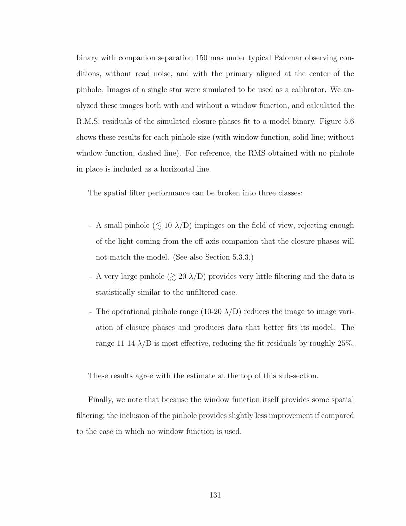
binary with companion separation 150 mas under typical Palomar observing con-
ditions, without read noise, and with the primary aligned at the center of the
pinhole. Images of a single star were simulated to be used as a calibrator. We an-
alyzed these images both with and without a window function, and calculated the
R.M.S. residuals of the simulated closure phases fit to a model binary. Figure 5.6
shows these results for each pinhole size (with window function, solid line; without
window function, dashed line). For reference, the RMS obtained with no pinhole
in place is included as a horizontal line.
The spatial filter performance can be broken into three classes:
- A small pinhole (. 10 λ/D) impinges on the field of view, rejecting enough
of the light coming from the off-axis companion that the closure phases will
not match the model. (See also Section 5.3.3.)
- A very large pinhole (& 20 λ/D) provides very little filtering and the data is
statistically similar to the unfiltered case.
- The operational pinhole range (10-20 λ/D) reduces the image to image vari-
ation of closure phases and produces data that better fits its model. The
range 11-14 λ/D is most effective, reducing the fit residuals by roughly 25%.
These results agree with the estimate at the top of this sub-section.
Finally, we note that because the window function itself provides some spatial
filtering, the inclusion of the pinhole provides slightly less improvement if compared
to the case in which no window function is used.
131
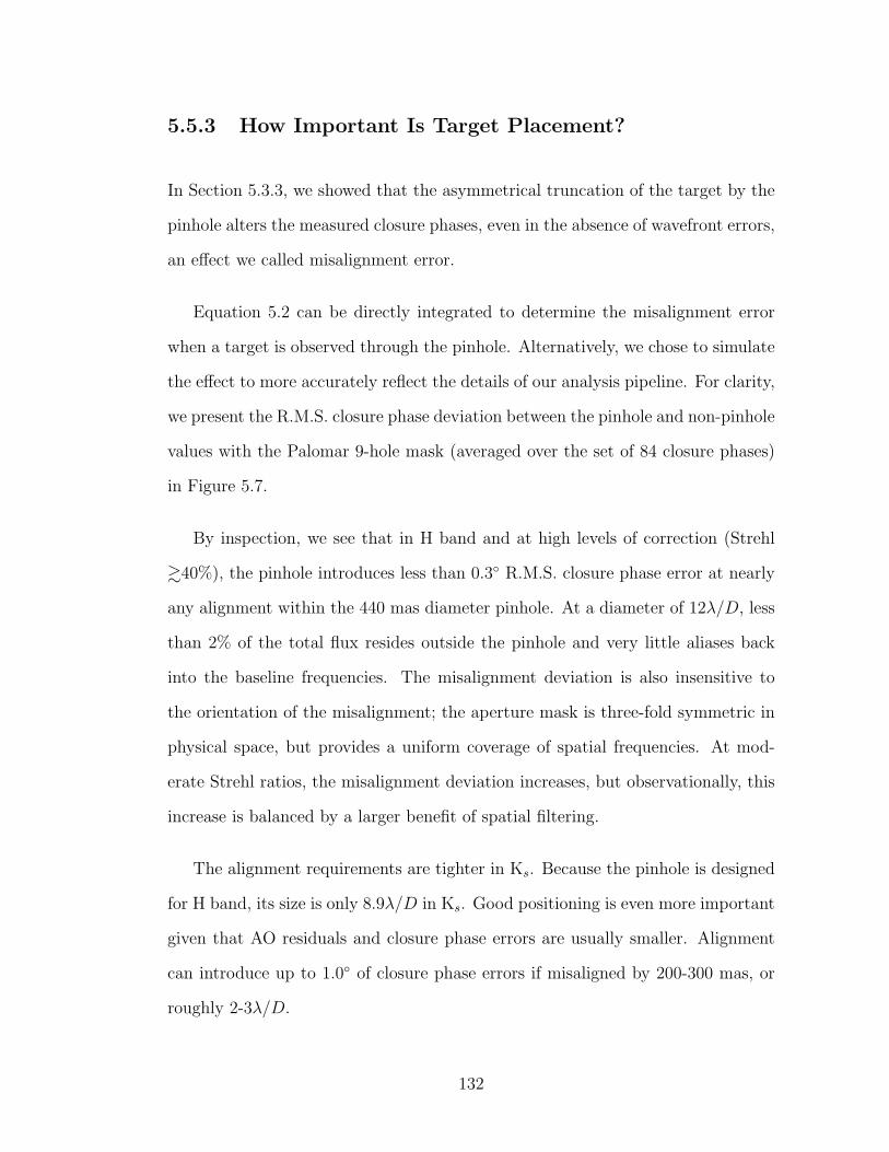
5.5.3 How Important Is Target Placement?
In Section 5.3.3, we showed that the asymmetrical truncation of the target by the
pinhole alters the measured closure phases, even in the absence of wavefront errors,
an effect we called misalignment error.
Equation 5.2 can be directly integrated to determine the misalignment error
when a target is observed through the pinhole. Alternatively, we chose to simulate
the effect to more accurately reflect the details of our analysis pipeline. For clarity,
we present the R.M.S. closure phase deviation between the pinhole and non-pinhole
values with the Palomar 9-hole mask (averaged over the set of 84 closure phases)
in Figure 5.7.
By inspection, we see that in H band and at high levels of correction (Strehl
&40%), the pinhole introduces less than 0.3◦ R.M.S. closure phase error at nearly
any alignment within the 440 mas diameter pinhole. At a diameter of 12λ/D, less
than 2% of the total flux resides outside the pinhole and very little aliases back
into the baseline frequencies. The misalignment deviation is also insensitive to
the orientation of the misalignment; the aperture mask is three-fold symmetric in
physical space, but provides a uniform coverage of spatial frequencies. At mod-
erate Strehl ratios, the misalignment deviation increases, but observationally, this
increase is balanced by a larger benefit of spatial filtering.
The alignment requirements are tighter in Ks. Because the pinhole is designed
for H band, its size is only 8.9λ/D in Ks. Good positioning is even more important
given that AO residuals and closure phase errors are usually smaller. Alignment
can introduce up to 1.0◦ of closure phase errors if misaligned by 200-300 mas, or
roughly 2-3λ/D.
132
The presence of a companion adds an additional misalignment error, although
this error will be attenuated by the secondary-primary contrast ratio. Therefore,
particularly for high contrast binaries, the misalignment errors provided here give
good rule-of-thumb indications of how well a target must be positioned within the
pinhole. Given that aperture masking observations at Palomar typically yield 1-2
degrees of closure phase, targets must be positioned close to the pinhole center
during Ks band observations.
Finally, we note that the percentage of blocked flux is a weak function of the
target alignment, and a strong function of the AO performance and size of the
direct imaging halo (Figure 5.2, right panel). In the observations of Section 5.6
which compare pinhole and non-pinhole observations, the percent loss of flux is a
measurable quantity. From the results of this plot, it is clear that large flux drops
can be attributed to momentary drops in AO performance or very large shifts
in alignment. Astrometric jitter on the scale of hundreds of mas is never seen.
Practically, if a series of images contains one or a few with large flux drops, and
the target was initially well aligned, then identifying large flux drops is a useful
proxy for excluding frames taken with poor AO performance.
5.5.4 Window Function: Optimal Size and the Palomar
9-Hole Mask
For our experiment, we use a super-Gaussian function, exp(−kx4), for its flat-top
and quickly tapering Fourier Transform. We describe the window function by the
size of its half width at half max, wpix, measured in pixels on the detector.
The optimal window function size finds the balance between eliminating read
133
noise and increasing redundancy noise. We present a measure of the effectiveness
of various window function sizes in the presence of various levels of read noise in
Figure 5.8.
We simulated one hundred images (256 x 256 in size) of a 10:1 binary with
companion separation 150 mas and of a calibrator in the same fashion as described
in Section 5.5.2 but without a pinhole in place. To each set of images we added
gaussian read noise with a per-pixel noise level ranging from 0.2% to 5.0% of
the peak intensity. (This corresponds to targets of 7th to 10th magnitude when
taking 6 second exposures on the PHARO detector.) The images were processed
with window functions of various sizes and we calculated the root mean squared
(RMS) residuals of fits to a model binary. In Figure 5.8 we plot the ratio of the
measured RMS with a window function to the same set of images without the
window function. For all levels of read noise an optimally sized window function
improves the model fits. We caution that, because the effect of read noise on closure
phases scales with image size, and the choice of default image size is arbitrary, the
results can only be evaluated qualitatively.
Several features are apparent.
First, the optimal window function is approximately λ/dsub, or ∼ 12λ/D for
the Palomar aperture mask, with tighter windows for the high noise cases; one
expects the optimal window size to be a function of the aperture mask. This
makes qualitative sense: The interferogram image is a set of interference fringes
under an Airy function envelope of characteristic size λ/dsub. One would expect
the optimal window function to crop out those pixels with signal to noise less than
one. Beyond λ/dsub, the intensity of the interferogram drops below a few percent
of its peak value, comparable to the read noise.
134
Second, too small a window function quickly adds redundancy noise into the
measurements. This turning point is near 0.5 λ/dsub.
Third, even in the absence of read noise, a window function decreases closure
phase noise (solid curve). This demonstrates the capacity of the window function
to spatial filter the wavefront phase noise, even though the improvement is only
about 3-4%.
To emphasize the utility of the window function as a spatial filter of wavefront
errors we simulated another set of images in which the wavefront is static over
the exposure. With only spatial variation of the wavefront, the window function
reduces closure phase errors by nearly 20% (Figure 5.9).
Misaligning the peaks of the window function and interferogram introduces a
tiny amount of closure phase error. Even an unrealistic misplacement of 10λ/D
(about 26 pixels on PHARO at 1.6µm) with a tight window of size 0.7 λ/dsub
produces an error below 0.06◦. This will likely on be relevant for observations
taken by space telescopes.
5.6 Observations
Between June 2008 and September 2009, we observed twenty-six single star targets
and four known binaries spanning infrared magnitudes between 6.0 and 9.0 using
the PHARO instrument on the Hale 200” Telescope at Palomar Observatory.
Each aperture masking observation was conducted with and without the pinhole
in place to compare the effectiveness and practicality of using the pinhole filter
during ground observing. An observing sequence consisted of sets of twenty images
135
(six second exposures) with the Palomar 9-hole aperture mask in several standard
infrared bands. Typically images were taken in a particular band with the pinhole
in place, then again with the pinhole removed, until the sequence of bands had
been taken. Similar observations of a calibrator were then taken. This was done to
minimize changes in seeing between comparison observations and to minimize the
effect of instrumental wavefront changes from slewing the telescope on calibration.
Care was taken to use identical detector configurations (position, etc) and to align
the target center of light at the center of the pinhole. This alignment procedure
added approximately two to five minutes additional overhead to each observation
set.
The aperture mask, data taking procedure, and custom IDL pipeline to analyze
aperture masking images have been previously described by Lloyd et al. (2006),
Kraus et al. (2008), and Bernat et al. (2010). The mean and variance of the closure
phases and amplitudes were calculated (across the set of images) and calibrated.
The calibrated closure phases were found by subtracting the calibrator closure
phases from those of the target; their errors were estimated by adding in quadrature
the errors of the targets and calibrator. The closure phase signal of a single star is
zero; deviations from zero may indicate the presence of a companion or result from
wavefront errors. The log-amplitudes are calibrated identically and are included
to determine if spatial filtering improves measurement of the amplitudes, but are
not used for the analysis of the binary candidates. Companions are located by
fitting the closure phase data set with a three parameter binary closure phase
model (separation distance, position angle, and contrast ratio) to minimize χ2.
The targets are bright enough that the per-pixel read noise is at or below a few
percent For the analysis that follows, we use the results of Section 5.5.4 and use a
136

window function with half-width at half-max of 1.0 λ/dsub (30.9 pixels in H band,
41.5 in Ks band).
5.6.1 Pinhole Stability and Target Alignment
Images of the pinhole were taken at several periods throughout the run, from
which its location on the detector can be measured. The location of the pinhole
remained accurate to less than two pixels for the entire run, with the exception
of two instances in which the Slit wheel appeared to lodge the pinhole at an
alternative location. This was easily repaired by putting the Slit wheel into its
’HOME’ position.
Explicit (direct) images of the target within the pinhole were taken only rarely.
However, the locations of the interferogram centers provided an accurate location
of the binary targets on the detector. Drift of the target was typically less than
one-half pixel during a set of twenty images (about two minutes). Comparison of
the target and pinhole locations indicate that our alignment was accurate to within
four pixels of the measured pinhole center. We conclude that the largest potential
source of misalignment error arises from the initial pointing accuracy within the
pinhole, and not jitter of the target or pinhole during data taking.
The effect of the pinhole was seen to alter several observables. Most directly,
when observing reference stars, the pinhole induced a drop of target flux by roughly
35% in H and 15% in Ks. The pinhole is located after the adaptive optics system
in the focal plane, hence these values reflect the percentage of the direct imag-
ing point spread function which falls outside the pinhole. These percentages are
consistent with the pinhole size and the level of AO performance (Strehl ratios of
137

approximately 10% in H and 30% in Ks). Binary targets show a similar drop in
flux despite their larger size, which we can take as an indication that their center
of light is well aligned.
Simulations and calculations using a sample of direct images show that the
percentage of blocked flux is a weak function of the target alignment, and so large
flux variations do not indicate a high level of astrometric jitter. Instead, this
percentage is a strong function of the AO performance (and size of direct imaging
halo). Low transmission (below 40%) well identified individual images blurred by
temporary drops in AO correction. High flux transmission well predicted good fits
to models (e.g. Figure 5.10).
5.6.2 Calibrators: Pinhole Filtering Produces Lower Clo-
sure Phase Variance and Higher Amplitudes
The use of the pinhole generally reduced the variance of closure phases and in-
creased the amplitudes for the observed single stars. These results are compared
to a set of simulated observations in Figure 5.11.
The closure phase standard deviation is reduced by 10 and 19 percent in H band
(1.6µm) and Ks band (2.2µm), respectively. A larger reduction is expected at the
longer wavelength, as the pinhole is relatively smaller and provides more aggressive
spatial filtering. Although not displayed, the root mean squared residuals of the
data fit to their model values also reduced by 10-20% indicating better calibrated
data. The pinhole filtering increases the visibility log-amplitude by 14 and 18
percent on the longest baselines at H band and Ks band, respectively. Each of
these confirm the spatial filter is reducing closure phase noise from sub-aperture
138
redundancy.
In both cases the simulation predicts a larger reduction in variance, although
the results across wavelengths are consistent. The simulation does not include
the time-variation of AO residuals during a single exposure, particularly slow tip-
tilt correction of the PALAO system (Bloemhof et al., 2001). This can produce
several interferograms in a dataset with large closure phase errors which cannot be
improved by spatial filtering.
5.6.3 Binaries: Lower Closure Phase Variance
We observed four previously characterized binaries with well defined orbits with
and without the pinhole in several bandpasses: GJ 164 (Martinache et al., 2009);
G 78-28 (Pravdo et al., 2006); GJ 623 (Martinache et al., 2007); and GJ 802B
(Ireland et al., 2008). The characterized orbits were used to predict the location of
each companion on the observing date using a Monte Carlo simulation to account
for the uncertainty of the orbital parameters. Each target was observed to obtain
twenty images (six second exposures) in several bandpasses in September 2009.
Three of the four known binaries were successfully resolved (Table 5.1). The high
contrast companion to GJ 802B could not be resolved at the correct separation
and contrast ratio.
GJ 164 was imaged for three sets near dawn with the pinhole and one set
without. All but the first sets of data suffered poor AO correction, were visibly
less sharp, and had flux levels drop by nearly 75%. The binary could be well
resolved in all three sets with the pinhole, but the later sets yield much worse fits
and larger systematic errors and are not used in the analysis. The fit parameters
139

to GJ 164 share a degeneracy with a spurious set of parameters (∆H = 0.030, at
nearly the same location), and limit the quality of parameter errors which can be
derived from the fit. Instead, the magnitude contrast was held fixed to the values
determined by Martinache et al. (2007). The observations of reference stars to
calibrate GJ 623 varied in AO correction and quality between pinhole and non-
pinhole measurements, and so this target is presented without calibration in order
to compare the two performances.
The median closure phase scatter (stochastic errors) decreased for each obser-
vation by roughly 20-25%, which indicates that the pinhole operated effectively to
minimize closure phase errors from AO residuals. However, the data fits to binary
models showed no decrease in R.M.S. residuals, whereas the fits to single star data
decreased by 10-20%. Of the eight total measurements, four showed an increase in
R.M.S., although only two Ks band observations increased by more than 10%. The
observations which increased in R.M.S. are those in which either the companions
was aligned far from the pinhole center, or the companion is comparatively bright.
We prefer to discuss this measurement in terms of the amount of unattributed
systematic error that needs to be added in quadrature to the stochastic errors to
yield the R.M.S. values, i.e., (R.M.S)2 =< σ2φ + σ2
sys >. This is listed in the next
to last column of Table 5.1. A systematic component of 1.0◦ specific to binary
targets would account for the discrepancy of performance.
Misalignment of the target within the pinhole contributes to the increased
residuals. Because each binary system could be resolved by direct imaging, the
targets were aligned with their center of light as close to the pinhole center as
could be accurately judged by eye. This necessarily placed each star off-center of
the pinhole. The astrometric alignment of each component can be inferred from
140
the center of the interferograms and is listed in Table 5.3. As discussed earlier,
the alignment of the components is determined by the original placement of the
observer and moves comparatively little during a set of images.
We simulated each binary with and within the pinhole displaced by the amounts
in Table 5.3. The atmospheric seeing was tuned to fit Strehl ratio estimates from
direct images taken throughout the night: 40% in Ks and Brγ bands, 15% in H and
CH4s bands, and 10% in J band. The astrometric jitter of the simulated images
was consistent to those observed (and less than 20 mas per twenty images for most
targets). Each simulation produced enough images until all errors reached a steady
state; the estimates of the misalignment error are included in the last column of
Table 5.1. Additional contributions from misaligned calibrators are not included.
Our calculation of the misalignment error requires knowledge of the absolute
positions of the pinhole and target components, and an accurate measure of the
point spread function. Given the small jitter of targets, our calculation is limited
by imperfect knowledge of the point spread function. Even still, the quality of
correction can fluctuate in timescales of minutes, as can be observed by viewing
successive direct images or other observables such as pinhole transmission (Figure
5.10). Given these assumptions, misalignment contributes systematic components
of 0.4-0.8◦ to the H and Ks band binary observations. We also note that simulations
demonstrate large & 1.0◦ alignment errors for slightly lower Strehl ratios (.10%
in H and .20% in Ks). These challenges instead warrant the development of an
observing strategy to calibrate alignment errors empirically.
The binary parameters measured with and without the pinhole, and those
predicted by the system orbits, are in good agreement. In each case, the spatial
filter data fit to slightly higher contrasts ratios (≈5%). This may indicate that the
141

Tab
le5.
1:O
bse
rvat
ion
ofK
now
nB
inar
ies
Wit
han
dW
ithou
tSpat
ial
Filte
r
Sep
arat
ion
Pos
.A
ng.
Con
tras
tB
est
Fit
Med
ian
Est
’dE
st’d
Bin
ary
Ban
d(m
as)
(deg
)∆
Mag
R.M
.S(◦
)σφ(◦
)C
alφsys(◦
)σalign(◦
)
GJ
164
H48
.7±
1.9
346.
5±
1.7
d4.
032.
11Y
3.4
H(S
PF
)48
.8±
1.5
343.
9±
0.9
d3.
331.
99Y
2.7
0.61
Pre
dic
teda
49.4±
2.2
348.
1±
10.1
1.83
5±
0.00
6Ks
46.8±
1.2
340.
3±
1.0
d3.
461.
20Y
3.2
Ks
(SP
F)
46.3±
0.7
341.
2±
1.2
d2.
160.
70Y
2.9
0.42
Pre
dic
teda
49.4±
2.2
348.
1±
10.1
1.72
1±
0.09
7
G78
-28
H10
1.7±
0.3
359.
2±
0.2
1.27
5±
0.01
02.
781.
16Y
2.5
H(S
PF
)10
2.6±
1.4
359.
6±
0.2
1.32
3±
0.01
53.
001.
09Y
2.8
0.68
Pre
dic
tedb
105.
0±
5.7
359.
3±
1.8
1.24±
0.07
Ks
103.
4±
0.3
359.
0±
0.1
1.22
1±
0.00
72.
680.
72Y
2.6
Ks
(SP
F)
104.
5±
0.2
359.
3±
0.1
1.22
1±
0.00
53.
600.
56Y
3.6
0.75
Pre
dic
tedb
105.
0±
5.7
359.
3±
1.8
1.14±
0.06
J10
1.4±
0.6
358.
7±
1.3
1.25
7±
0.02
17.
603.
12Y
6.9
J(S
PF
)10
0.8±
0.6
358.
5±
0.2
1.26
3±
0.01
15.
802.
55Y
5.2
0.24
Pre
dic
tedb
105.
0±
5.7
359.
3±
1.8
1.24±
0.07
GJ
623
CH
4 s28
2.3±
1.4
176.
3±
0.4
2.79
8±
0.05
03.
381.
90N
2.8
CH
4 s(S
PF
)27
7.3±
3.0
176.
2±
0.2
2.82
9±
0.51
3.43
1.65
N3.
00.
75P
redic
tedc
279.
1±
1.2
177.
4±
0.7
2.86
0±
0.03
9Ks
277.
1±
0.4
176.
5±
0.1
2.67
5±
0.01
42.
350.
45N
2.3
Ks
(SP
F)
280.
7±
0.2
176.
6±
0.7
2.78
0±
0.10
1.9
0.30
N1.
90.
46P
redic
tedc
279.
1±
1.2
177.
4±
0.7
2.72
0±
0.01
4B
rγ27
9.1±
0.3
176.
2±
0.7
2.66
4±
0.01
20.
940.
42N
0.8
Brγ
(SP
F)
279.
4±
0.4
176.
5±
0.1
2.77
8±
0.00
91.
280.
33N
1.2
0.63
Pre
dic
tedc
279.
1±
1.2
177.
4±
0.7
2.72
0±
0.01
4
Mea
sure
men
tsof
thre
eknow
nbin
ary
syst
ems
wit
han
dw
ithou
tth
epin
hol
efilt
er(S
PF
).aSpat
ial
filt
erin
gre
duce
sth
em
edia
nsc
atte
rof
clos
ure
phas
em
easu
rem
ents
inal
lca
ses.
bT
he
med
ian
resi
dual
bet
wee
nth
edat
aan
db
est
fitt
ing
model
does
not
incr
ease
when
usi
ng
the
pin
hol
e.c
An
esti
mat
eof
the
syst
emat
icer
ror
due
toa
mis
alig
nm
ent
of3
pix
els.
See
text
for
dis
cuss
ion.
Not
e:T
arge
tG
J80
2is
excl
uded
from
this
table
.
142
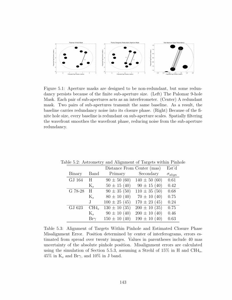
Palomar 9-Hole Mask
-3 -2 -1 0 1 2 3Projected Pupil Position (meters)
-3
-2
-1
0
1
2
3
Pro
jecte
d P
up
il P
ositio
n (
me
ters
)
b
Poorly Designed (Redundant) Aperture Mask
-3 -2 -1 0 1 2 3Projected Pupil Position (meters)
-3
-2
-1
0
1
2
3
Pro
jecte
d P
up
il P
ositio
n (
me
ters
)
b
b’
Sub-Aperture Scale Redundancy
-0.5 0.0 0.5 1.0 1.5 2.0 2.5Projected Pupil Position (meters)
-1.5
-1.0
-0.5
0.0
0.5
1.0
1.5
Pro
jecte
d P
up
il P
ositio
n (
me
ters
)
Figure 5.1: Aperture masks are designed to be non-redundant, but some redun-dancy persists because of the finite sub-aperture size. (Left) The Palomar 9-holeMask. Each pair of sub-apertures acts as an interferometer. (Center) A redundantmask. Two pairs of sub-apertures transmit the same baseline. As a result, thebaseline carries redundancy noise into its closure phase. (Right) Because of the fi-nite hole size, every baseline is redundant on sub-aperture scales. Spatially filteringthe wavefront smoothes the wavefront phase, reducing noise from the sub-apertureredundancy.
Table 5.2: Astrometry and Alignment of Targets within Pinhole
Distance From Center (mas) Est’dBinary Band Primary Secondary σalign
GJ 164 H 90 ± 50 (60) 140 ± 50 (60) 0.61Ks 50 ± 15 (40) 90 ± 15 (40) 0.42
G 78-28 H 90 ± 35 (50) 110 ± 35 (50) 0.68Ks 80 ± 10 (40) 70 ± 10 (40) 0.75J 100 ± 25 (45) 170 ± 23 (45) 0.24
GJ 623 CH4s 130 ± 10 (35) 200 ± 10 (35) 0.75Ks 90 ± 10 (40) 200 ± 10 (40) 0.46Brγ 150 ± 10 (40) 190 ± 10 (40) 0.63
Table 5.3: Alignment of Targets Within Pinhole and Estimated Closure PhaseMisalignment Error. Position determined by center of interferograms, errors es-timated from spread over twenty images. Values in parentheses include 40 masuncertainty of the absolute pinhole position. Misalignment errors are calculatedusing the simulation of Section 5.5.3, assuming a Strehl of 15% in H and CH4s,45% in Ks and Brγ, and 10% in J band.
143

(a) AO Corrected Phase (b) Overlay of Aperture Mask
(c) AO + Spatial Filter Phase (d) Overlay of Aperture Mask
Figure 5.2: Effect of the pinhole filter on sub-aperture scale phase variation. a)AO corrected wavefront phase. Small scale spatial inhomogeneities are apparent.b) The AO corrected wavefront with an overlay of the aperture mask. Notice thatthe wavefront phase is inhomogeneous within the sub-aperture. c) AO correctedwavefront after spatial filtering. The small scale features are smoothed out; thewavefront exhibits structure with a characteristic scale close to that of the sub-apertures. d) Within each sub-aperture, the spatially filtered phase is much moreuniform.
144
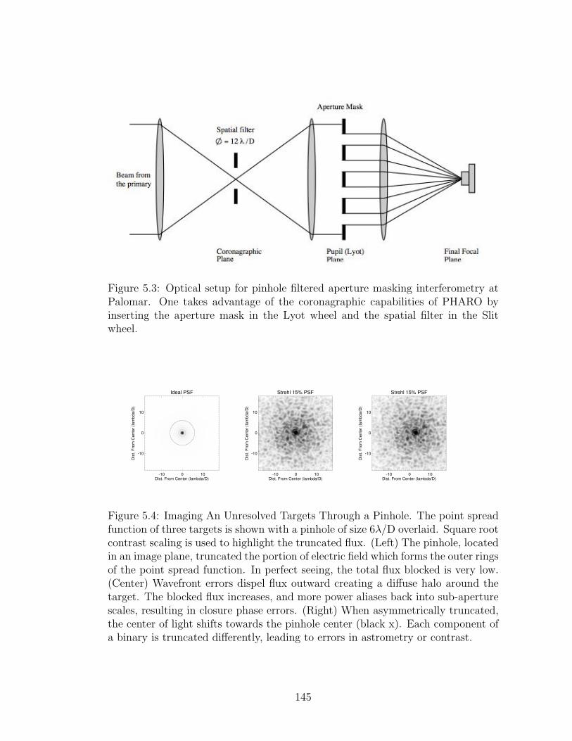
Figure 5.3: Optical setup for pinhole filtered aperture masking interferometry atPalomar. One takes advantage of the coronagraphic capabilities of PHARO byinserting the aperture mask in the Lyot wheel and the spatial filter in the Slitwheel.
-10 0 10Dist. From Center (lambda/D)
-10
0
10
Dis
t. F
rom
Ce
nte
r (la
mb
da
/D)
Ideal PSF
-10 0 10Dist. From Center (lambda/D)
-10
0
10
Dis
t. F
rom
Ce
nte
r (la
mb
da
/D)
Strehl 15% PSF
-10 0 10Dist. From Center (lambda/D)
-10
0
10
Dis
t. F
rom
Ce
nte
r (la
mb
da
/D)
Strehl 15% PSF
Figure 5.4: Imaging An Unresolved Targets Through a Pinhole. The point spreadfunction of three targets is shown with a pinhole of size 6λ/D overlaid. Square rootcontrast scaling is used to highlight the truncated flux. (Left) The pinhole, locatedin an image plane, truncated the portion of electric field which forms the outer ringsof the point spread function. In perfect seeing, the total flux blocked is very low.(Center) Wavefront errors dispel flux outward creating a diffuse halo around thetarget. The blocked flux increases, and more power aliases back into sub-aperturescales, resulting in closure phase errors. (Right) When asymmetrically truncated,the center of light shifts towards the pinhole center (black x). Each component ofa binary is truncated differently, leading to errors in astrometry or contrast.
145
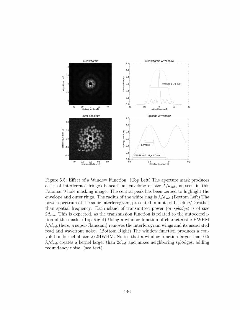
-40 -20 0 20 40Units of lambda/D
-40
-20
0
20
40
Un
its o
f la
mb
da
/DInterferogram Interferogram w/ Window
-40 -20 0 20 40Units of lambda/D
0.0
0.2
0.4
0.6
0.8
1.0
1.2
Win
do
w F
un
ctio
n
FWHM (~2 L/d_sub)
-1.0 -0.5 0.0 0.5 1.0Baseline (Units of D)
-1.0
-0.5
0.0
0.5
1.0
Ba
se
line
(U
nits o
f D
)
Power Spectrum
2 d_sub
Splodge w/ Window
-0.1 0.0 0.1 0.2Baseline (Units of D)
0.0
0.2
0.4
0.6
0.8
1.0
1.2
Sp
lod
ge
Am
plit
ud
e
FWHM ~ 0.5 L/d_sub Case
L/FWHM
Figure 5.5: Effect of a Window Function. (Top Left) The aperture mask producesa set of interference fringes beneath an envelope of size λ/dsub, as seen in thisPalomar 9-hole masking image. The central peak has been zeroed to highlight theenvelope and outer rings. The radius of the white ring is λ/dsub.(Bottom Left) Thepower spectrum of the same interferogram, presented in units of baseline/D ratherthan spatial frequency. Each island of transmitted power (or splodge) is of size2dsub. This is expected, as the transmission function is related to the autocorrela-tion of the mask. (Top Right) Using a window function of characteristic HWHMλ/dsub (here, a super-Gaussian) removes the interferogram wings and its associatedread and wavefront noise. (Bottom Right) The window function produces a con-volution kernel of size λ/2HWHM. Notice that a window function larger than 0.5λ/dsub creates a kernel larger than 2dsub and mixes neighboring splodges, addingredundancy noise. (see text)
146
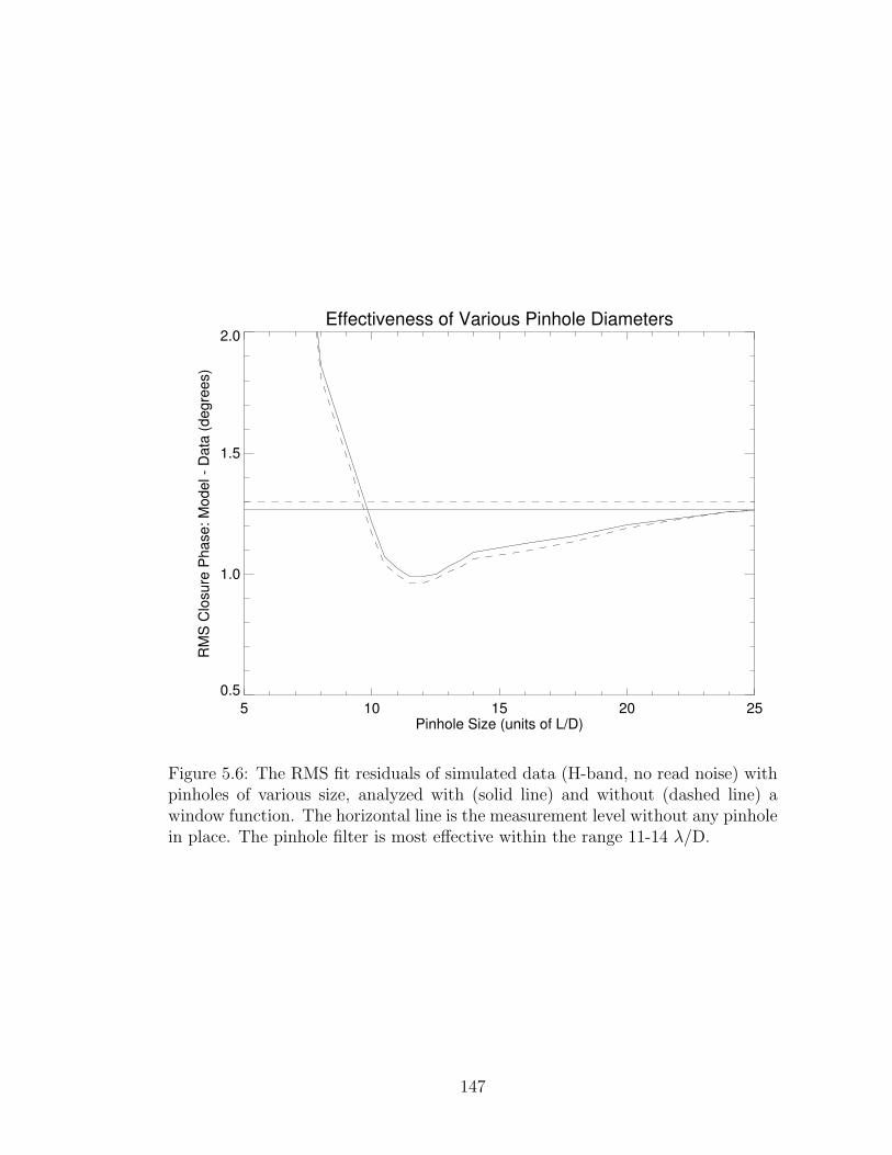
Effectiveness of Various Pinhole Diameters
5 10 15 20 25Pinhole Size (units of L/D)
0.5
1.0
1.5
2.0
RM
S C
losu
re P
ha
se
: M
od
el -
Da
ta (
de
gre
es)
Figure 5.6: The RMS fit residuals of simulated data (H-band, no read noise) withpinholes of various size, analyzed with (solid line) and without (dashed line) awindow function. The horizontal line is the measurement level without any pinholein place. The pinhole filter is most effective within the range 11-14 λ/D.
147
companion flux was skewed closer to the pinhole edge and its flux truncated by a
few percent more, which is consistent with the measured locations of the objects
within the pinhole (Table 5.3). No bias was found in the relative astrometry.
Binary parameter errors decrease in proportional to the closure phase errors,
and indicate that one can use a pinhole to measure binary parameters more pre-
cisely. Detection contrast also scales with closure phase errors, and indicate pinhole
measurements can provide an increase of contrast by 20-25%. However, it must be
noted that our practice of scaling the closure phase errors until the χ2 of the best
fit is unity, because the data residuals did not improve, will partially counteract
the other gains in precision.
5.7 Summary of Results and Conclusions
In this text, we discussed spatial wavefront variation on the scale of NRM sub-
apertures, which contributes to closure phase errors we called sub-aperture redun-
dancy noise. We proposed that quasi-static wavefront errors on the scale of the
sub-aperture, which evolve over hundreds of seconds or with telescope movement,
give rise to the limitations of aperture masking calibration. Through simulations
and direct observation we have shown that the use of a pinhole filter effectively re-
duces sub-aperture spatial variation and can reduce closure phase errors, increase
visibility amplitudes, and lead to better calibration and higher detection contrasts.
With a simple premise, we estimate the optimal pinhole size to be dspf ≈ D/dsub
in units of λ/D, or about 12λ/D for the Palomar 9-hole mask. We confirm this
result using a detailed simulation of the Palomar aperture masking experiment and
show that the operational pinhole size ranges from 11 to 14λ/D. Smaller pinholes
148
reject enough light from off-axis companions to alter the measured closure phases.
Larger pinholes provide little spatial filtering.
Because the pinhole is not a perfect low-pass filter, the truncation of off-axis
targets aliases power back into phase at sub-aperture scales. This introduces clo-
sure phase errors of its own, both systematic and stochastic. Using simulated
observations over a wide range of correction (Strehl ratio of 10-100%), we show
that a misalignment of the target by 200 mas introduces 0.3-1.0◦ degrees of system-
atic closure phase, which we have termed misalignment error. We propose several
methods for the calibration of this component although none are undertaken in
this experiment. As a result, the effectiveness of pinhole technique is limited by
the accuracy with which targets can be aligned within the center of the pinhole.
We installed a pinhole of size 0.779 arcsec (12λ/D at 1.6µm) in the Slit wheel
focal plane of the PHARO instrument on the Hale 200” Telescope at Palomar
Observatory. Using this pinhole we observed twenty single unresolved stars and
three well characterized binaries with and without the pinhole in a selection of
standard near infrared bands. The AO system provided moderate correct: Strehl
∼5-15% in H band and ∼20-40% in Ks band.
Observations of unresolved stars showed that the pinhole reduced the stochas-
tic variation of closure phases by 10-25% from one image to the next, and visibility
amplitudes increased. R.M.S. residuals to model fits decreased by a similar factor.
Each shows that increasing sub-aperture coherence decreases closure phase redun-
dancy noise. Lower fit residuals indicate that calibration improved, and that the
aperture masking calibration limit is partially attributable to small scale quasi-
static wavefront errors. Furthermore, detection contrasts scales proportional to fit
residuals, indicating an increase in detection contrast of 10-25%.
149

The modest increase in closure phase signal to noise when the pinhole is used
suggests that the spectrum of wavefront errors contains relatively little power on
the smallest spatial-scales within the sub-aperture. Additionally, the smallest scale
variations which cycle multiple times within a single sub-aperture tend to produce
redundancy noise that averages out. The leading source of spatial redundancy
noise, both quasi-static instrumental and residual atmospheric wavefront errors, is
more likely low-order Zernike modes (i.e, ’phase slopes’) across the sub-apertures.
Section 5.10 presents a more detailed derivation of sub-aperture spatial redundancy
in terms of the spatial structure of the sub-aperture wavefront.
Simulations of these observations, when compared, predict a slightly larger
benefit from the pinhole filtering. As discussed in Section 5.3.2, temporal varia-
tions of the baseline phase within a single exposure leads to a sort of temporal
redundancy noise which cannot be removed by closure phases of the pinhole filter.
Furthermore, the slow response of the Palomar AO tip-tilt mirror (5 Hz) gives rise
to full aperture scale wavefront residuals which evolve on the order of a fraction
of an exposure. The baseline phase changes these residuals induce contribute to
the overall variation of the closure phases from one image to the next (though not
calibration errors). The simulation did not include temporal variations of the AO
residuals, and as a result gives the impression that the pinhole is more effective
at reducing stochastic closure phase noise (50% vs. 20%). Indeed, these results
imply that temporal variation of the wavefront phase is a large source of closure
phase variance with the current PALAO system.
We observed three well characterized binary systems to determine how the
pinhole influences the astrometric and photometric characterizations of discovered
systems. The measured binary parameters were consistent with those acquired
150
without the pinhole, and those predicted by the measured orbital parameters of
the system. No bias was found in the astrometry (i.e., binaries did not tend
towards shorter separations with the pinhole), however contrast ratios with the
pinhole tended to be a few percent fainter. Our alignment technique placed the
system center of light near the pinhole center, and the light of the companion is
preferentially blocked by this arrangement. Better positioning of the target would
likely remedy this bias.
Although closure phase stochastic errors decreased by 20-25%, binary data
acquired with the pinhole provided no better fits to data, and suggest that binary
targets observed with the pinhole contain an additional 1.0◦ systematic error. After
simulating these observations with and without the pinhole, we conclude that the
systematic component arises from the off-center alignment of a resolved target.
Simulations demonstrate large & 1.0◦ alignment errors at low Strehl ratios (.10%
in H band and .20% in Ks).
Binary parameter errors and detection contrast both decrease in proportion to
the closure phase errors, and indicate that one can achieve more precisely measured
binary parameters and higher contrasts (20-25%) with the pinhole. However, our
practice of scaling closure phase errors to account for data residuals will partially
counteract the other gains in precision and requires calibration of the misalignment
error in the high contrast or high precision regime.
Finally, we showed that multiplying the images by an apodized window function
acts to reduce the effects of wavefront error similar to a spatial filter. We found
that the optimal window function has a half-width at half-max of about λ/dsub,
with smaller window functions favored for targets in which read noise is higher.
151
5.8 Discussion
5.8.1 A Strategy for Future Pinhole Observations
In light of this investigation, the pinhole can prove effective in two scenarios.
When seeing or correction is poor, and closure phase observations do not reach the
calibration limit, a pinhole filter will clearly provide higher signal to noise closure
phases and more efficient data taking.
At the other extreme, the pinhole may be valuable for improving very-high
Strehl ratio (&80%) observations with extreme-AO systems. The high spatial
frequencies filtered by the pinhole contribute a larger proportion of the overall
wavefront errors in this scenario. The pinhole could be optimally tuned to the
AO actuator size, much larger, and alignment requirements would be substantially
relaxed. Most importantly, the aliasing of high spatial frequency content into sub-
aperture scale phase errors is a higher order effect of the wavefront (Poyneer &
Macintosh, 2004). At very high levels of correction, the aliased power is a smaller
component of closure phase errors.
We can arrive at a rough estimate of a pinhole performance on extreme-AO sys-
tems by simulating a higher-order AO system, such as the 3368-actuator Palomar
3000 system (P3K, Dekany et al. (2007)). As mentioned earlier, our simulation
does not account for the sluggish tip-tilt correct of the current Palomar system
and over predicted the pinhole performance as a result. The P3K system will have
upgraded response by using the current 241 actuator system to perform low-order
correction, and thus provide more stable correction. Using the specifications of
this system, we simulated a 10:1 binary separated by 150 mas in H band under
152
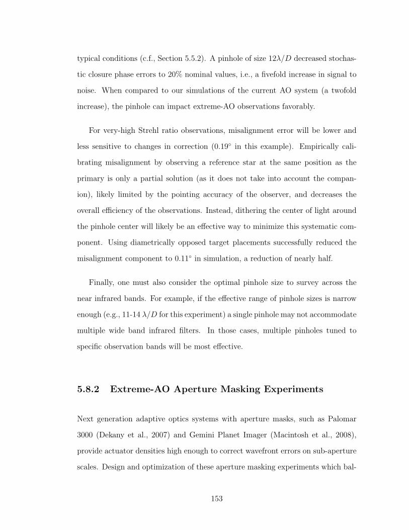
typical conditions (c.f., Section 5.5.2). A pinhole of size 12λ/D decreased stochas-
tic closure phase errors to 20% nominal values, i.e., a fivefold increase in signal to
noise. When compared to our simulations of the current AO system (a twofold
increase), the pinhole can impact extreme-AO observations favorably.
For very-high Strehl ratio observations, misalignment error will be lower and
less sensitive to changes in correction (0.19◦ in this example). Empirically cali-
brating misalignment by observing a reference star at the same position as the
primary is only a partial solution (as it does not take into account the compan-
ion), likely limited by the pointing accuracy of the observer, and decreases the
overall efficiency of the observations. Instead, dithering the center of light around
the pinhole center will likely be an effective way to minimize this systematic com-
ponent. Using diametrically opposed target placements successfully reduced the
misalignment component to 0.11◦ in simulation, a reduction of nearly half.
Finally, one must also consider the optimal pinhole size to survey across the
near infrared bands. For example, if the effective range of pinhole sizes is narrow
enough (e.g., 11-14 λ/D for this experiment) a single pinhole may not accommodate
multiple wide band infrared filters. In those cases, multiple pinholes tuned to
specific observation bands will be most effective.
5.8.2 Extreme-AO Aperture Masking Experiments
Next generation adaptive optics systems with aperture masks, such as Palomar
3000 (Dekany et al., 2007) and Gemini Planet Imager (Macintosh et al., 2008),
provide actuator densities high enough to correct wavefront errors on sub-aperture
scales. Design and optimization of these aperture masking experiments which bal-
153
ance sub-aperture size and number against adaptive optics correction and the limi-
tations of systematics requires a more detailed understanding of how sub-aperture
wavefront errors impact closure phases, and where resources should be focused.
This work provides one such investigation, and Section 5.10 presents a formalism
for this optimization. Extreme-AO systems are anticipated to provide highly stable
correction down to scales of 8 cm and thus may motivate smaller and additional
sub-apertures, providing more spatial frequency coverage and resolution. This
balance will depend on the spatial and temporal power spectra of the corrected
wavefront residuals, and this data should be accumulated.
154
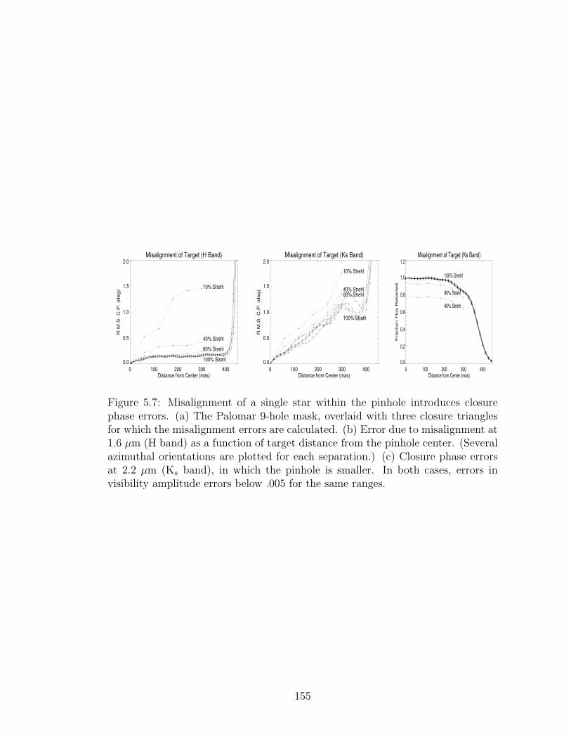
Misalignment of Target (H Band)
0 100 200 300 400Distance from Center (mas)
0.0
0.5
1.0
1.5
2.0
R.M
.S. C
.P. (d
eg)
10% Strehl
40% Strehl
80% Strehl
100% Strehl
Misalignment of Target (Ks Band)
0 100 200 300 400Distance from Center (mas)
0.0
0.5
1.0
1.5
2.0R
.M.S
. C
.P. (d
eg)
10% Strehl
40% Strehl80% Strehl
100% Strehl
Misalignment of Target (Ks Band)
0 100 200 300 400Distance from Center (mas)
0.0
0.2
0.4
0.6
0.8
1.0
1.2
Fraction F
lux R
eta
ined
40% Strehl
80% Strehl
100% Strehl
Figure 5.7: Misalignment of a single star within the pinhole introduces closurephase errors. (a) The Palomar 9-hole mask, overlaid with three closure trianglesfor which the misalignment errors are calculated. (b) Error due to misalignment at1.6 µm (H band) as a function of target distance from the pinhole center. (Severalazimuthal orientations are plotted for each separation.) (c) Closure phase errorsat 2.2 µm (Ks band), in which the pinhole is smaller. In both cases, errors invisibility amplitude errors below .005 for the same ranges.
155

Window Function Decreases Closure Phase RMS
0 1 2 3Window Size (units of Lambda/d_sub)
0.0
0.5
1.0
1.5
Clo
su
re P
ha
se
RM
S:
with
WF
/ w
ith
ou
t W
F
Figure 5.8: Window functions reduce closure phase error from read noise. Thesecurves, from top to bottom, display the reduction in RMS closure phase errorwhen read noise is 0% (top, solid), 0.2%, 0.4%, 0.6%, 1.0%, and 5.0% (bottom,dotted) of the peak image intensity. The optimal window function is typically ofsize ∼ λ/dsub, or ∼ 12λ/D for the Palomar aperture mask, with higher read noisefavoring tighter window functions. Smaller window functions quickly add largeamounts of redundancy noice. (See text.) Note: Even with no read noise (solidcurve), a window function reduces closure phase errors, indicating that the windowfunction provides an effect similar to spatially filtering the wavefront.
156
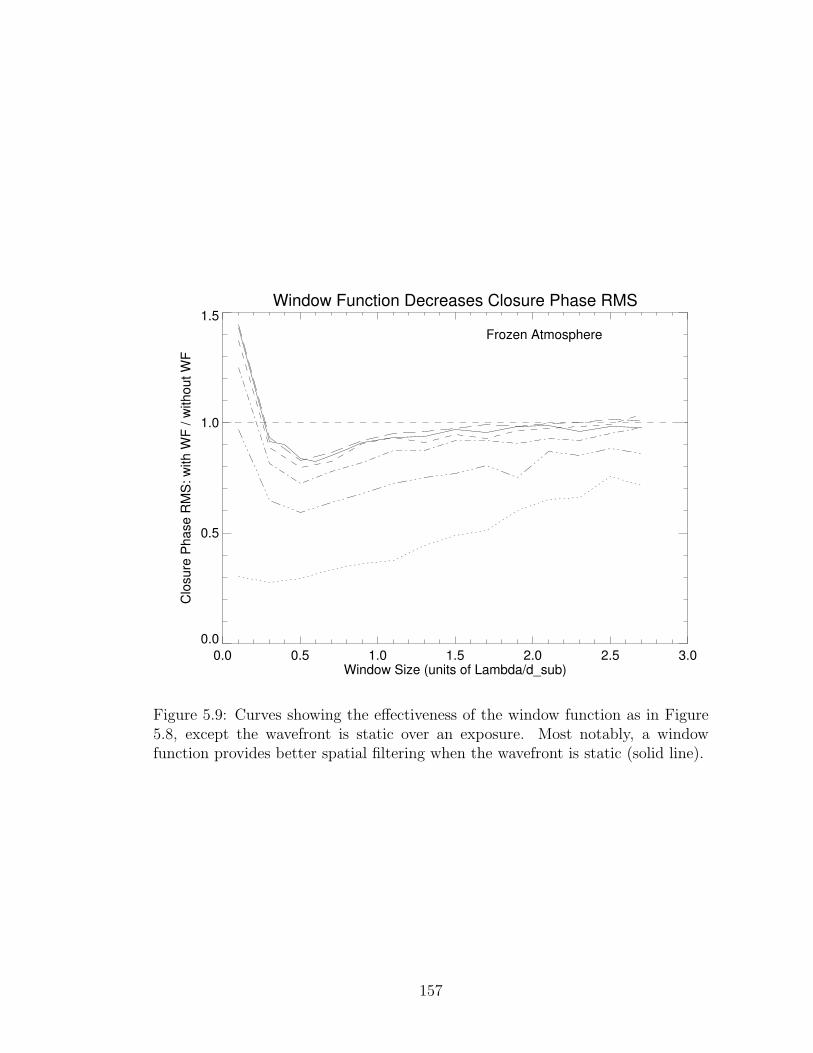
Window Function Decreases Closure Phase RMS
0.0 0.5 1.0 1.5 2.0 2.5 3.0Window Size (units of Lambda/d_sub)
0.0
0.5
1.0
1.5
Clo
su
re P
ha
se
RM
S:
with
WF
/ w
ith
ou
t W
F
Frozen Atmosphere
Figure 5.9: Curves showing the effectiveness of the window function as in Figure5.8, except the wavefront is static over an exposure. Most notably, a windowfunction provides better spatial filtering when the wavefront is static (solid line).
157
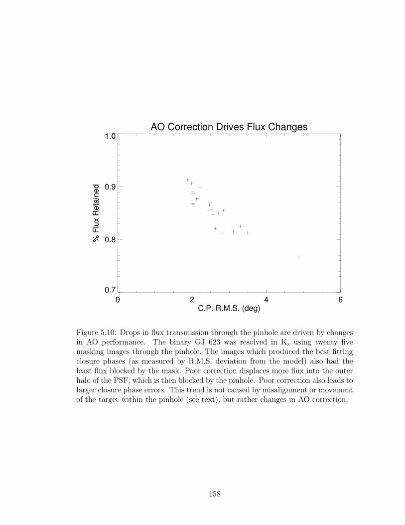
AO Correction Drives Flux Changes
0 2 4 6C.P. R.M.S. (deg)
0.7
0.8
0.9
1.0
% F
lux R
eta
ined
Figure 5.10: Drops in flux transmission through the pinhole are driven by changesin AO performance. The binary GJ 623 was resolved in Ks using twenty fivemasking images through the pinhole. The images which produced the best fittingclosure phases (as measured by R.M.S. deviation from the model) also had theleast flux blocked by the mask. Poor correction displaces more flux into the outerhalo of the PSF, which is then blocked by the pinhole. Poor correction also leads tolarger closure phase errors. This trend is not caused by misalignment or movementof the target within the pinhole (see text), but rather changes in AO correction.
158
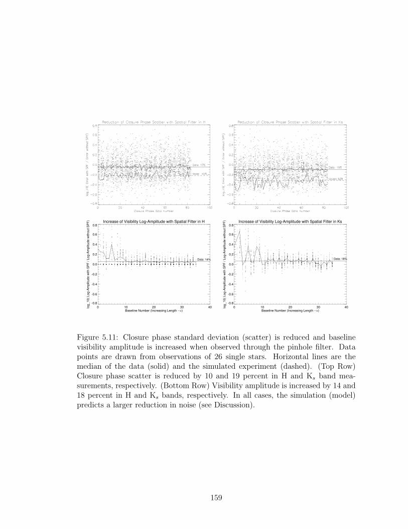
Increase of Visibility Log-Amplitude with Spatial Filter in H
0 10 20 30 40Baseline Number (Increasing Length -->)
-0.8
-0.6
-0.4
-0.2
0.0
0.2
0.4
0.6
0.8
log_10(
Log-A
mplit
ude w
ith S
PF
/ L
og-A
mplit
ude w
ithout S
PF
)
Data: 14%
Increase of Visibility Log-Amplitude with Spatial Filter in Ks
0 10 20 30 40Baseline Number (Increasing Length -->)
-0.8
-0.6
-0.4
-0.2
0.0
0.2
0.4
0.6
0.8lo
g_10(
Log-A
mplit
ude w
ith S
PF
/ L
og-A
mplit
ude w
ithout S
PF
)
Data: 18%
Figure 5.11: Closure phase standard deviation (scatter) is reduced and baselinevisibility amplitude is increased when observed through the pinhole filter. Datapoints are drawn from observations of 26 single stars. Horizontal lines are themedian of the data (solid) and the simulated experiment (dashed). (Top Row)Closure phase scatter is reduced by 10 and 19 percent in H and Ks band mea-surements, respectively. (Bottom Row) Visibility amplitude is increased by 14 and18 percent in H and Ks bands, respectively. In all cases, the simulation (model)predicts a larger reduction in noise (see Discussion).
159
ACKNOWLEDGEMENTS
We thank the staff and telescope operators of Palomar Observatory for their
support and many nights of assistance at the Hale Telescope. The authors appre-
ciate the effort of the reviewers, who provided valuable advice on the clarity and
depth of this text. This material is based upon work supported by the National
Science Foundation under Grant No. AST-0705085. The Hale Telescope at Palo-
mar Observatory is operated as part of a collaborative agreement between Caltech,
JPL, and Cornell University. This publication makes use of data products from
the Two Micron All Sky Survey, which is a joint project of the University of Mas-
sachusetts and the Infrared Processing and Analysis Center/California Institute of
Technology, and is funded by the National Aeronautics and Space Administration
and the National Science Foundation.
5.9 Pinhole Filtering: Inteferometry
Observing through a pinhole alters the measured complex visibility of a point
source even in the absence of any wavefront aberrations. This analysis assumes
that the Fraunhofer approximation applies, i.e., that the electric field in the image
plane is the Fourier Transform of the phasor of the wavefront phase in the pupil
frame. We assume no wavefront aberrations, including those from optical errors
and central obscurations.
The optical path is shown in Figure 5.3. We denote the electric field at the
telescope aperture with the subscript a and the electric field after spatially filtering
with the subscript spf . The coordinates in the image plane are ~θ; all angles are
measured in units of λ/D. We assume the pinhole has angular diameter dspf and
160
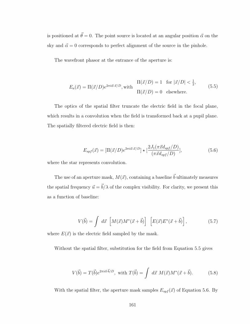
is positioned at ~θ = 0. The point source is located at an angular position ~α on the
sky and ~α = 0 corresponds to perfect alignment of the source in the pinhole.
The wavefront phasor at the entrance of the aperture is:
Ea(~x) = Π(~x/D)e2πi~α·~x/D,withΠ(~x/D) = 1 for |~x/D| < 1
2,
Π(~x/D) = 0 elsewhere.(5.5)
The optics of the spatial filter truncate the electric field in the focal plane,
which results in a convolution when the field is transformed back at a pupil plane.
The spatially filtered electric field is then:
Espf (~x) = [Π(~x/D)e2πi~α·~x/D] ? [2J1(π~xdspf/D)
(π~xdspf/D)], (5.6)
where the star represents convolution.
The use of an aperture mask, M(~x), containing a baseline~b ultimately measures
the spatial frequency ~u = ~b/λ of the complex visibility. For clarity, we present this
as a function of baseline:
V (~b) =
∫d~x[M(~x)M∗(~x+~b)
] [E(~x)E∗(~x+~b)
], (5.7)
where E(~x) is the electric field sampled by the mask.
Without the spatial filter, substitution for the field from Equation 5.5 gives
V (~b) = T (~b)e2πi~α·~b/D, with T (~b) =
∫d~x M(~x)M∗(~x+~b). (5.8)
With the spatial filter, the aperture mask samples Espf (~x) of Equation 5.6. By
161
recognizing that convolution with e2πi~α·~x/D leads to a Fourier Transform, doing so
before substitution yields:
Vspf (~b) = T (~b)
∫d~θ Π[~θ/dspf ]× e2πi~θ·~b/D ×
[2J1(π|~θ − ~α|)π|~θ − ~α|
]2
(5.9)
In the limit of an infinite pinhole, the integral converges to the value
T (~b)e2πi~α·~b/D.
We can extend use this approach to include arbitrary pupil-plane phase errors
which arise prior to propagation through the pinhole system. In the presence of
inhomogeneous phase in the pupil plane, eiφ(x), Equation 5.6 becomes
Espf (~x) = [Π(~x/D)e2πi~α·~x/Deiφ(~x)] ? [2J1(π~xdspf/D)
(π~xdspf/D)], (5.10)
Repeating the steps above, the complex visibility is written as:
Vspf (~b) = T (~b)
∫d~θ Π[~θ/dspf ]× e2πi~θ·~b/D × PSF [~θ − ~α], (5.11)
with
PSF [~θ] =
∣∣∣∣∫ d~x e2πi~θ·~x/D Π(~x/D)eiφ(~x)
∣∣∣∣2 . (5.12)
5.10 Spatial Structure of Closure Phase Redundancy Noise
Within this work it has been stated that non-zero closure phases can be introduced
by sub-aperture phase inhomogeneities, and that producing a more coherent phase
across a sub-aperture will lead to better measurements. While this statement has
been studied at length for the seeing limited case (see, e.g., Readhead et al. (1988)
and Nakajima et al. (1989)), no approach has been put forward tailored for NRM
observations with adaptive optics.
162
Spatially filtering the smallest scale structure of wavefront inhomogeneities is
one approach for producing a more coherent sub-aperture wavefront. Next gener-
ation adaptive optics systems, such as Palomar 3000 and Gemini Planet Imager,
provide actuator densities high enough to correct wavefront errors on sub-aperture
scales. Additionally, pupil-reimaging techniques, such as Serabyn et al. (2006) have
successfully concentrated the set of actuators onto a subset of the pupil, thus pro-
viding increased actuator densities and achieving very high Strehl ratios (&92%)
with conventional adaptive optics systems on a smaller aperture. Sparse NRM
techniques generally cover less than 10% of the full aperture; one can conceive of
future experiments which concentrate adaptive optics correction to sub-aperture
wavefront modes.
Design and optimization of new aperture masking experiments, which balance
sub-aperture size and number against adaptive optice correction and the limita-
tions of systematics, requires a more detailed understanding of how sub-aperture
wavefront errors impact closure phases, and where resources should be focused.
This section presents a formalism for this optimization, and establishes redun-
dancy noise in the semi-coherent sub-aperture case. We also find that decomposing
the sub-aperture wavefronts in Zernike modes is convenient for accommodating the
conventions used in adaptive optics.
Zernike Modes
By describing the inhomogeneities of a static wavefront with Zernike modes, we will
investigate the spatial noise sources of aperture masking interferometry and show
that the primary noise source for closure phases comes from only the structure of
the wavefront within the sub-aperture.
163
A static wavefront can be decomposed into Zernike modes, Zmn (x), a set of
orthonormal functions which naturally describe perturbations to spherical wave-
fronts. The polynomials are defined on a unit circle, and must be scaled to fit the
aperture. We use the definitions of Noll (1976) which normalize the polynomials
such that they are orthnormal, i.e.,
∫d2x Z0
0(x) = 1 (5.13)∫d2x Zm
6=0(x) = 0 (5.14)∫d2x Zm
n (x)Zsr (x) = δnr δms (5.15)
Although Kolmogorov turbulence distributes power into even very high order
Zernike modes, most of the power falls into the low order modes. To facilitate
discussion of these modes, we present their names: Z0, piston; Z±11 , tip/tilt; Z0
2 ,
defocus; and Z±22 astigmatism.
5.10.1 Baseline Visibility Measurement
The measured visibility of the incoming wavefront, eiφ(~x), through an aperture
M(~x) is:
V (~r) =
∫ texp
0
dt
∫d~x ei[φ(~x+~r,t)−φ(~x,t)]M(~x+ ~r)M(~x). (5.16)
If the aperture, M(~x), is a two-hole mask with unit area circular sub-apertures
separated by a distance~b, then the visibility of the corresponding baseline simplifies
to
164
V (~b) =
∫ texp
0
dt
∫sub−
aperture 1
d~x ei[φ(~x+~b,t)−φ(~x,t)]. (5.17)
In the limit of zero exposure time, the instantaneous baseline visibility is
V (~b) =
∫sub−
aperture 1
d~x ei[φ(~x+~b)−φ(~x)]. (5.18)
Notice that the integral is carried out over the set of redundant baselines. For
a so called non-redundant mask, the baselines stretching between sub-aperture
centers are redundant only within the sub-aperture. The baseline phasors, not
phases, add.
One could decompose the wavefront over each sub-aperture into Zernike modes.
We define a sub-aperture at ~x = 0 by φ1(~x) =∑
n,m amn Zmn (~x), with amn =∫
d~x φ1(~x)Zmn (~x). The wavefront over the sub-aperture at ~x = ~b, φ2(~x), is de-
composed into Zernike coefficients bmn .
Referring to Equation 5.18, we note that the quantity φ(~x+~b)− φ(~x) is itself,
then, a sum of Zernike terms. We denote the coefficients of this difference by
αmn ≡ amn − bmn .
We also note that if the apertures are far separated (with respect to the adaptive
optics decorrelation length), then we can assume the Zernike coefficients of the
two sub-apertures are uncorrelated. This implies, then, that the coefficient αmn has
the same statistics as the single aperture coefficients, with a standard deviation
increased by√
2.
This allows us to represent the visibility by
165
V (~b) =
∫sub−
aperture 1
d~x exp
[i∑n,m
αmn Zmn (~x)
]. (5.19)
Taylor expanding the exponential the sub-aperture yields
V (~b) =
∫sub−
aperture 1
d~x δ(~x)+
[i∑n,m
αmn Zmn (~x)
]− 1
2
[∑n,m
αmn Zmn (~x)
]2
+O(α3) (5.20)
and integrating the Zernike polynomials yields
V (~b) = 1 + iα00 −
1
2
∑n,m
(αmn )2 +O(α3). (5.21)
The leading order error in the visibility phase is α00 = a0
0 − b00, the difference of
the sub-aperture Z00 (piston) modes. The piston mode is the average phase above
the sub-aperture. However, the second and third order terms are not generally
zero: the visibility phase is not generally equal to the average phase above one sub-
aperture minus the average phase of the other sub-aperture. This is the source of
redundancy noise.
The leading order term that affects the amplitude of V (~b) is equivalent to the
mean wavefront variance over the sub-aperture.
5.10.2 Instantaneous Closure Phase
In this sub-section we show that closure phases remove sub-aperture piston, but
that high order terms persist.
We define the bispectrum, B(~b1,~b2), as
166

B(~b1,~b2) ≡ V (~b1) V (~b2) V ∗(~b1 +~b2). (5.22)
The argument (complex phase) of the bispectrum is the closure phase.
For three sub-apertures centered at ~x = 0, ~b1, and ~b1 +~b2, we can follow the
same progression that lead to equation 5.21 for the bispectrum
B(~b1,~b2) =
∫sub−
aperture 1
d~x d~x′ d~x′′ ei[φ(~x+~b1)−φ(~x)] ei[φ(~x′+~b1+~b2)−φ(~x′+~b1)] ei[φ(~x′′)−φ(~x′′+~b1+~b2)],
(5.23)
where each integral occurs over the domain of the sub-aperture centered at ~x = 0
only.
We cast the bispectrum in terms of the sub-aperture Zernike modes of the three
sub-apertures. We define the three sets of Zernike coefficients over the apertures
centered at ~x = 0, ~x = ~b1, and ~x = ~b1 +~b2 as amn , bmn , and cmn , respectively.
Again, we recognize that the bispectrum is the difference between Zernike de-
compositions, and denote the difference coefficients as αmn ≡ bmn −amn , βmn ≡ cmn −bmn ,
and γmn ≡ amn − cmn . Their definitions lead to the identity: αmn + βmn + γmn = 0.
B(~b1,~b2) =
∫sub−
aperture 1
d~x exp
[i∑n,m
αmn Zmn (~x) + βmn Z
mn (~x′) + γmn Z
mn (~x′′)
]. (5.24)
Taylor expanding the exponential yields the following terms:
167
0th Order : 1 (5.25)
1st Order : i∑n,m
∫αmn Z
mn (~x) + βmn Z
mn (~x′) + γmn Z
mn (~x′)
= α00 + β0
0 + γ00 = 0 (5.26)
2nd Order : −1
2
∑n,m,r,s
∫αmn α
srZ
mn (~x)Zs
r (~x) + αmn βsrZ
mn (~x)Zs
r (~x′) + αmn γ
srZ
mn (~x)Zs
r (~x′′)
βmn αsrZ
mn (~x′)Zs
r (~x) + βmn βsrZ
mn (~x′)Zs
r (~x′) + βmn γ
srZ
mn (~x′)Zs
r (~x′′) +
γmn αsrZ
mn (~x′′)Zs
r (~x) + γmn βsrZ
mn (~x′′)Zs
r (~x′) + γmn γ
srZ
mn (~x′′)Zs
r (~x′′)(5.27)
= −α00β
00 − α0
0γ00 − β0
0γ00 −
1
2
∑n,m
[(αmn )2 + (βmn )2 + (γmn )2
](5.28)
= −1
2
∑n 6=0,m
[(αmn )2 + (βmn )2 + (γmn )2
](5.29)
Equation 5.28 is obtained by directly integrating the Zernike terms over x,x′,
and x′′. The last line pulls the n = 0 terms out of the sum and uses the identify
12(α0
0 + β00 + γ0
0)2 = 0 to remove these term. We see that to second order of αmn ,
βmn , and γmn , the error in the closure phase is zero. The bispectrum amplitude and
phase are both unaffected by sub-aperture piston.
To account for the errors in closure phase, we must go to third order. In a
similar process of integrating over Zernike terms, regrouping piston terms outside
the summation, and application of the identity α00 + β0
0 + γ00 = 0, we find the third
order term to be
Third Order : − i6
∑n6=0,m,r 6=0,s,v 6=0,w
∫d~x αmn α
srα
wv Z
mn (~x)Zs
r (~x)Zwv (~x)+ βmn β
srβ
wv & γmn γ
srγ
wv terms,
(5.30)
Piston terms again drop out, as do cross terms such as αmn βsrβ
wv Z
mn (~x)Zs
r (~x′)Zv
w(~x′).
168
Although this integral is difficult to solve analytically, we can use several rela-
tions to restrict the set of Zernike indices which produce non-zero integrals. We
recognize that, when integrated over the unit circle, the angular part of the Zernike
polynomials restricts either one or three of the azimuthal indices to be even. This
implies the leading term of the sequence to be α±11 α±1
1 α0,±22 . If we assume the long
baseline approximation such that α has the same statistical behavior as the sub-
aperture coefficients, then the leading term of closure phase noise is the product
of two sub-apertures’ tip/tilts and one sub-aperture’s defocus/astigmatism.
Equation 5.30 provides a valuable avenue for estimating the impact of sub-
aperture adaptive optics. For example, the PALM3K extreme-AO system actuator
spacing is 8.1 centimeters (Dekany et al., 2007). Using the current 9-hole NRM
mask with 42 cm sub-apertures, corresponding to roughly 21 actuators per sub-
aperture, the PALM3K system will be able to actively control the first twenty one
terms of the expression above (see, for example Nakajima & Haniff (1993)). This
provides a useful metric for balancing sub-aperture size again other considerations,
such as calibration and quasi-static wavefront limitations, photon noise, and trade-
offs between smaller sub-apertures and increasing the number of sub-apertures.
169
CHAPTER 6
SYNTHESIS AND CONCLUSIONS
This body of work provides the technical underpinnings of Non-Redundant
Aperture Masking Interferometry with Adaptive Optics and contributes to a young
but growing literature on this subject. By enabling high-contrast infrared imaging
at diffraction-limited separations, the combined technique allows for the resolu-
tion of brown dwarfs and exoplanet systems that cannot be observed by any other
method. One of the most valuable uses of this technique is in the detection of
short period brown dwarf binary systems, which lead to model-independent mea-
surements of brown dwarf masses. These, in turn, can be used to empirically test
and refine current brown dwarf evolution and atmospheric models which also set
the foundation for our understanding of massive Jupiter exoplanets.
Enhancing the precision of NRM with AO by upgraded AO systems and re-
fined analysis techniques will enable even higher contrasts and the resolution of
exoplanets directly. The scientific potential of NRM exoplanet imaging includes
the mass measurement of exoplanets and the full-characterization of planetary sys-
tems imaged by coronagraphic surveys (e.g., Hinkley et al. (2011)). For nearby
stars, the NRM working angle corresponds to planet-star separations of much less
than 5 AU, and provides a unique method to image exoplanets formed in situ by
core accretion (Kraus et al., 2009).
The goal of this final chapter is to review and synthesize the results of the
presented studies. Section 1 reviews the new methods that have been developed
in this work, Section 2 reviews the major results, Section 3 explores the possible
future work that could be motivated by these studies, and Section 4 concludes with
the broader implications of this work.
170

6.1 Refinement of the NRM with AO Technique: Results
Completing this work required several new numerical and statistical methods for
using NRM with AO to detect faint companions. The early successes of NRM with
AO imaging were driven by the immediate effectiveness of the closure phase method
for producing observations uninhibited by quasi-static wavefront errors. The de-
tection of moderate-contrast companion can be readily identified (e.g., Martinache
et al. (2007); Pravdo et al. (2006), and NRM provides much higher precision than
direct imaging alone. But the forward model approach (see Chapter 3), when
employed before this work, often produced spurious detections of faint compan-
ions, sometimes even at the many-sigma level. This over confidence arose in part
because of inherent correlations of the closure phase signals that were not taken
into account (c.f. Kulkarni (1989)); this is not to be confused by correlations of
measurement error, which can be handled by a covariant matrix. By developing
a simple Monte Carlo simulation that tests the forward model fits against sim-
ulated observations bootstrapped directly from the data, we now have tools to
confidently search for unknown, high-contrast companions. The simulation also
inherently incorporates measurement noise and calibration errors (and their cor-
relations), which makes the the simulation a more robust choice for calculating
contrast detection limitations (Chapter 4). The simulation has also been used by
Zimmerman et al. (2011) (of which I am a contributing author), which will pub-
lish the first NRM images taken by an Integral Field Spectrograph and dedicated
exoplanet instrument.
More broadly, my studies in this work aim to mix empirical analysis tools with
theoretical foundations to extract more precise information from current NRM im-
ages, and to reach higher contrast. Chapter 4 described a novel, intuitive, empirical
171
method for averaging closure phases that resulted a 2-4 fold increase in measure-
ment precision over what would have been derived by conventional averaging of
closure phases of bispectra.
Chapter 5 asserts that NRM is calibration-limited by quasi-static wavefront
errors on the sub-aperture scale, and describes precisely how these errors alter clo-
sure phases and bispectra. Upcoming extreme-AO systems will push observations
far enough into the calibration limit that individual modes of sub-aperture wave-
front errors may be discernible in the closure phase data. Developing higher-order
calibration methods may enable closure phases to be calculated that remove the
impact of some sub-aperture scale wavefront errors, in much the same way that
current radial velocity surveys extend to lower velocities by accurately parameter-
izing the point spread function response to telescope flexure. These same tools will
aid in the design of future aperture masking experiments that optimally alleviate
noise from AO residuals and instrumental effects. These new masks will balance
sub-aperture size and number against adaptive optics stability and actuator den-
sity. This balance will depend on the spatial and temporal power spectra of the
corrected wavefront residuals, and a formalism for doing so it presented.
6.2 Refinement of the NRM with AO Technique: Future
Work
By far, the greatest advances in NRM for the near term will arise from new NRM-
equipped exoplanet imagers with extreme-AO systems, e.g., Project 1640 at Palo-
mar (Hinkley et al., 2009), the Gemini Planet Imager (Macintosh et al., 2008),
and SPHERE on VLT (Beuzit et al., 2006). These instruments also feature In-
172
tegral Field Spectrographs capable of taking narrow-band images across multiple
wavelengths simultaneously. As discussed in Chapter 1, the inherent dependence
of quasi-static speckles behavior on wavelength allows one to distinguish true com-
panions from quasi-static speckles.
Much of the focus in the high-contrast imaging community is currently directed
toward obtaining higher contrast with coronagraphs behind extreme-AO and by
invoking speckle deconvolution algorithms that eliminate many of the quasi-static
speckles at wide separations (beyond 0.5 arcseconds; e.g., Crepp et al. (2010)).
Early speckle deconvolution algorithms anticipate to increase detection contrast
by a factor of 20 (Hinkley et al., 2010).
Narrow-band IFS NRM images, also allows one to construct algorithms anal-
ogous to speckle deconvolution that deconvolve closure phase errors, e.g., differ-
ential closure phases or differential spatial frequency phases. In the case of NRM
phase deconvolution, one aims to exploit the linear relationship between baseline
phase errors and inverse wavelength that one would expect to arise from physically
induced pupil-plane phase errors (i.e., ∆φ = ∆x/λ). In order to develop a relation-
ship between closure phase, pupil-plane phase errors, and wavelength, one needs
a more sophisticated understanding of how higher mode wavefront phase errors
affect closure phases (i.e., Section 5.10 to Chapter 5). The joint effort of closure
phases and deconvolution algorithms are complementary methods for mitigating
the effect of quasi-static wavefront errors.
Zimmerman et al. (2010), of which I am a contributing author, will publish
the first IFS NRM data, acquired by the Project 1640 instrument. Our analysis
reveals strong, positive correlations (¿ 0.80) between closure phase errors of various
channels, on par with those found by Crepp et al. (2010) for coronagraphic images.
173
This indicates that deconvolution algorithms can reduce closure phase errors. We
estimate a reduction by 5-10x per channel and a corresponding increase in detec-
tion contrast. While the AO correction provided by the PALAO system is not
high enough to produce the simple, linear relationship just discussed, the recently
commissioned extreme-AO system PALM3K is likely to do so. (It is important
to stress that developing more exacting algorithms to extract closure phases from
NRM images is crucial for these techniques to be effective. In my analysis of
the Zimmerman et al. (2010) data, redesigned extractions methods and diligent
awareness of systematic errors enabled clean deconvolution.)
Additionally, the spatial frequencies measured by an NRM are a function of
wavelength; hence, each channel of an IFS measures unique signals, increase the
total spatial frequency coverage by a factor of roughly twenty in the wavelength
limit, without considering chromatic techniques. The technique of IFS NRM, when
used with the current AO system and the Project 1640 instrument, has achieved an
estimated detection contrast of 1000:1 (∆M∼7.5) or higher at the diffraction limit.
The Project 1640 coronagraph performance is anticipated to increase by more
than tenfold after upgrading to the Palomar extreme-AO system and enabling the
precision wavefront control device of the instrument (Hinkley et al., 2010). Based
on these specifications, NRM with the Project 1640 instrument may reach as high
as 104:1 contrasts (∆M∼10.0).
Finally, one consequence of IFS NRM imaging is that it makes an excellent
tool for diagnosing instrumental misalignments and wavelength dependent errors,
which can, in turn, aid coronagraphic observations. For example, my analysis of
the Zimmerman et al. (2010) NRM images found evidence of a small tilt of the
mask in the Lyot wheel. Also, the dependence of the mask transmission function
174

on wavelength allows for a robust, independent determination of the central wave-
length of each channel with a single image. This scaling relation is a necessary
parameter of speckle deconvolution algorithms (e.g., Crepp et al. (2010), Figure
5) and crucial for extracting precise spectra from IFS images (E. Rice, private
communication). It is worth noting that the scaling relation may change as the
telescope moves, since the IFS lenslets alters the point spread function reaching the
detector. In other words, the scaling relation may be change from target to target,
and NRM provides an efficient way to calibrate this concurrent with coronagraph
observations.
For these reasons, this is a very exciting time for high-contrast NRM imaging,
and certainly deserves further attention in subsequent studies with more advanced
equipment.
6.3 Study of Brown Dwarf Binaries using LGSAO: Results
NRM is most sensitive to companions between λ/2D and 4λ/D, corresponding
to angular separations of 50 to 400 mas in the Ks infrared band (2.2µm). When
providing good correction, NRM with LGSAO has been shown to reach 102:1
(∆Ks=5.0) contrasts at the diffraction limit (Dupuy et al., 2009). The enhanced
contrast and resolution of NRM with LGSAO makes the technique a formidable
tool for resolving low mass brown dwarf (T dwarfs) companions to nearby field
brown dwarfs, particularly to enable high precision mass measurements (Chapter
2).
In Chapter 4, I used NRM in conjunction with the Palomar Laser Guide Star
Adaptive Optics system (LGSAO, Roberts et al. (2008)) to survey sixteen nearby
175
field brown dwarfs for companions. Due to the proximity of nearby field brown
dwarfs, the combined technique reached physical projected separations ranging
from 0.6-8.0 AU for most of the survey targets; this was the first imaging survey
to probe for companions to brown dwarfs shortward of 3 AU and the first NRM
with LGSAO survey at Palomar. Setbacks with the LGSAO system hampered the
observing, but despite the setbacks the survey reached contrasts of ∆Ks=1.5-2.5
outward of 100 mas. These results benefited greatly from the enhanced closure
phase averaging mentioned in the previous subsection.
In addition to seeking a subset of brown dwarf companions suitable for dynam-
ical mass measurements, the imaging survey can glean insights into the formation
process of brown dwarfs. The companion fraction of brown dwarfs is proposed
to be low (≈ 15%) and peaked within a narrow separation range, 3-10 AU (Bur-
gasser et al., 2008), little conclusive results are known for separations less than 3
AU. Using preliminary evidence compiled from irregular and sparse radial velocity
datasets, several authors suggested that at least as many brown dwarfs may reside
shortward of 3 AU (Jeffries & Maxted, 2005; Pinfield et al., 2003; Chappelle et al.,
2005). Such interesting statistical results may suggest that the brown dwarf binary
formation mechanism is different than that for solar type binaries (Burgasser et al.,
2007). The NRM with LGSAO imaging survey is one of the first observationally
complete surveys of the brown dwarf companion fraction at these separations.
The survey detected four candidate binaries with moderate to high confidence
(90-98%), including two with projected physical separations less than 1.5 AU.
This may indicate that tight-separation binaries contribute more significantly to
the binary fraction than currently assumed, consistent with the preliminary ra-
dial velocity results. One companion resides within the formal diffraction limit,
176
and one companion orbits a target previously imaged as part of a Hubble Space
Telescope companion search. All four candidates suggest brown dwarf masses and
the candidate status of all four targets can be immediately resolved by NRM with
LGSAO imaging on the Keck Telescope. The short projected separations of the
systems indicate a favorable likelihood that masses of the brown dwarfs can be
obtained within a few years.
6.4 Study of Brown Dwarf Binaries using LGSAO: Future
Work
Concurrent with the NRM with LGSAO for brown dwarf binaries were the LGSAO
direct imaging surveys of Konopacky et al. (2010) and Dupuy et al. (2010) (and
references within). Taken together, the set has more than tripled the number of
late-M, L, and T dwarf binaries with dynamical mass measurements. was the
dynamical mass measurement survey of several authors.
Based on direct measurements of their luminosities and total masses, evolution
model radii give effective temperatures that are inconsistent with those from model
atmosphere fitting of observed spectra by 100-300 K (the ’temperature problem’).
Evolutionary models also underpredict the luminosities for the only binary with an
independent age measurement by a factor of ∼2 (the ’luminosity problem’), which
implies that model-predicted substellar masses may be systematically too large.
Evolutionary models are also still untested at early ages (.100 Myr).
To tackle the ’temperature problem,’ it must first be determined whether the
discrepancy arises from systematic errors within the atmospheric models or incor-
177

rect estimated radii in the evolutionary models. This can be directly tested with
future discoveries of late-M and brown dwarf eclipsing binaries, as the tempera-
ture offset corresponds to a substantial radius difference (15-20%) (Dupuy et al.,
2010). Furthermore, infrared photometry has been shown to be a poor proxy for
effective temperature, particularly when visible photometry or a partial SED is
unavailable (Konopacky et al., 2010). In this respect, the low-resolution infrared
spectra of brown dwarfs obtained by Integral Field Spectrographs, combined with
dynamical mass measurements, will be valuable. Currently, no IFS instruments
are commissioned for telescopes with LGSAO systems. However, observations of
the two browns dwarfs resolvable with NGS AO, GJ 802b and GJ 581B (both from
Palomar), can be pursued.
Additionally, campaigns to image brown dwarfs in young systems (i.e., favor-
able contrasts between brown dwarfs and stellar primaries) can be pursued with
new high-contrast and IFS instruments, this would also move forward the test of
evolutionary models at young ages. Furthermore, because young systems have
constrained ages, comparisons of dynamical masses and model-implied masses will
begin to identify the nature of the ’luminosity problem’
Finally, continued observing of the currently known brown dwarf binaries with
LGSAO will increase the precision of the mass measurements. These binaries
have typical uncertainties larger than 30% (larger for the smallest mass brown
dwarfs) and are limited by relative astronomy of their orbits (as opposed to parallax
distance). Continued observation, especially with the improved relative astronomy
and photometry of NRM and LGSAO at Keck Telescope, can lead to truly high
precision mass and photometry measurements.
178
6.5 Future Explorations: Probing Evolution and Forma-
tion of Brown Dwarfs and Massive Jupiter Exoplanets
Within this work, the uncertainty of brown dwarfs atmospheric and evolution
models (and by extension, giant exoplanets) have been discussed at length, and
empirical tests have been discussed, proposed, and carried out. Dynamical mass
measurements, along with precise photometry, has been regularly discussed as a
major empirical test. The extensions of these models to planetary masses, in
concert with observations, will provide insights into the mass, radius, structure,
temperature, and metallicity of the exoplanets. In this section, I discuss how
these soon to be discovered massive Jupiter exoplanets can form and arrive at
their observed location, and I propose a method and survey for testing theories of
planetary formation.
6.5.1 New Paradigms of Planet Formation Driven by Di-
rect Imaging
The Jupiter-sized planets detected so far are radically different than the gas giant
planets in our solar system. Radial velocity and transit surveys detect hot Jupiters
with orbital periods of a few days; directly imaged planet-like companions have
been found out beyond even 50 AU, e.g., HR 8799 (Marois et al., 2010). These
detections have motivated sweeping changes to the paradigms of planet formation
and migration (Ida & Lin, 2004; Boss, 2001). More broadly, dozens of newly
discovered planetary systems outward 5-10 AU are anticipated after first light of
dedicated exoplanet imagers begin coronagraphic surveys (Beichman et al., 2010).
179
Core accretion occurs most rapidly at the ice line (2-8 AU), and characteris-
tically produces metal-enriched planets . 5MJ(Marcy et al., 2005). Subsequent
migration inward explains the short period hot-Jupiters, including the planet den-
sities measured by transits. At large separations, the timescales of formation are
too slow. Thus, wide-separated planets must be formed in situ by an alternative
method, such as gravitation instability (most prominent beyond 10 AU), or migrate
outward after formation near the ice line. Migration outward, either by planetes-
imals in the disk or massive inner planets, occurs on timescales of 50-100 Myrs
(Reipurth et al., 2007). The two mechanisms are predicted to yield different dis-
tributions of planetary mass, star-planet separation, luminosity, and metallicity.
Testing these theories has not yet been possible because of a lack of observable
data. The detection of well-characterized planetary systems around youthful stars,
including massive inner planets, before migration can occur, will be a key to testing
formation mechanisms (Hinkley et al. (2010), and references within).
6.5.2 A Growing Population of Nearby, Young Stars
Recently, great effort has been put into extending the membership of nearby, young
moving group associations in both the Northern and Southern hemisphere, includ-
ing several with median distances closer than 40 pc and ages less than 50 Myr.
Additionally, efforts are underway to identify new GK-type members, with a new-
membership rate of dozens per year (Zuckerman, 2004; Schlieder & Lepine, 2010).
The detection of full planetary systems around these stars provides a unique way
to test formation predictions.
With an inner working angle of 0.300” (10 AU @ 35 pc), the Gemini Planet
Imager and Project 1640 coronagraphs are unable to probe planets formed within
180
about 10 AU, including those formed in situ by core accretion. NRM provides a
complement to coronagraph observations. The working angle of NRM at shortward
infrared wavelengths is 0.040-0.400” (1-13 AU), and both exoplanet instruments
will be equipped with NRM masks. Used jointly, NRM and Coronagraphs explore
the full planetary architecture outward of roughly 1 AU.
This combination of targets and techniques opens up exoplanet searches to
massive inner planets, planets near the ice line, and planets formed in situ by bona
fide core accretion. Probing at these separations is not possible by radial velocity
because of stellar variability of youthful targets. It should be noted that such
a survey complements ongoing NRM companion searches in the Upper Scorpius
star-forming region. At an age of 5 Myrs, the region is ideal for planet searches,
but its distance (140 pc) limits detections to beyond 7 AU even with NRM (Kraus
et al., 2008).
6.5.3 Feasibility of the Survey with Exoplanet Instruments
and NRM
NRM provides the highest contrast of any technique at the diffraction-limited, and
one of the core motivations of this dissertation has been to refine the technique
of NRM to reach contrasts high enough to detect massive Jupiter exoplanets with
these next generation instruments.
The foremost factor influencing the detection of massive Jupiter planets at close
separations with NRM is that the host star must be bright enough to function as a
natural guide star. Currently, the Gemini Planet Imager and Project 1640 require
I band magnitudes ¡ 8-9 in order to use extreme-AO (Macintosh et al., 2008;
181
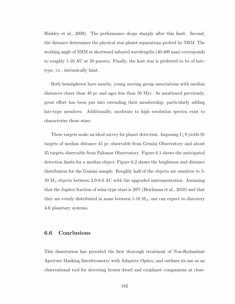
Hinkley et al., 2009). The performance drops sharply after this limit. Second,
the distance determines the physical star-planet separations probed by NRM. The
working angle of NRM at shortward infrared wavelengths (40-400 mas) corresponds
to roughly 1-10 AU at 20 parsecs. Finally, the host star is preferred to be of late-
type, i.e., intrinsically faint.
Both hemispheres have nearby, young moving group associations with median
distances closer than 40 pc and ages less than 50 Myr. As mentioned previously,
great effort has been put into extending their membership, particularly adding
late-type members. Additionally, moderate to high resolution spectra exist to
characterize these stars.
These targets make an ideal survey for planet detection. Imposing I ¡ 9 yields 91
targets of median distance 45 pc observable from Gemini Observatory and about
35 targets observable from Palomar Observatory. Figure 6.1 shows the anticipated
detection limits for a median object; Figure 6.2 shows the brightness and distance
distribution for the Gemini sample. Roughly half of the objects are sensitive to 5-
10 MJ objects between 2.0-8.0 AU with the upgraded instrumentation. Assuming
that the Jupiter fraction of solar-type stars is 20% (Beichman et al., 2010) and that
they are evenly distributed in mass between 1-10 MJ , one can expect to discovery
4-6 planetary systems.
6.6 Conclusions
This dissertation has provided the first thorough treatment of Non-Redundant
Aperture Masking Interferometry with Adaptive Optics, and outlines its use as an
observational tool for detecting brown dwarf and exoplanet companions at close-
182
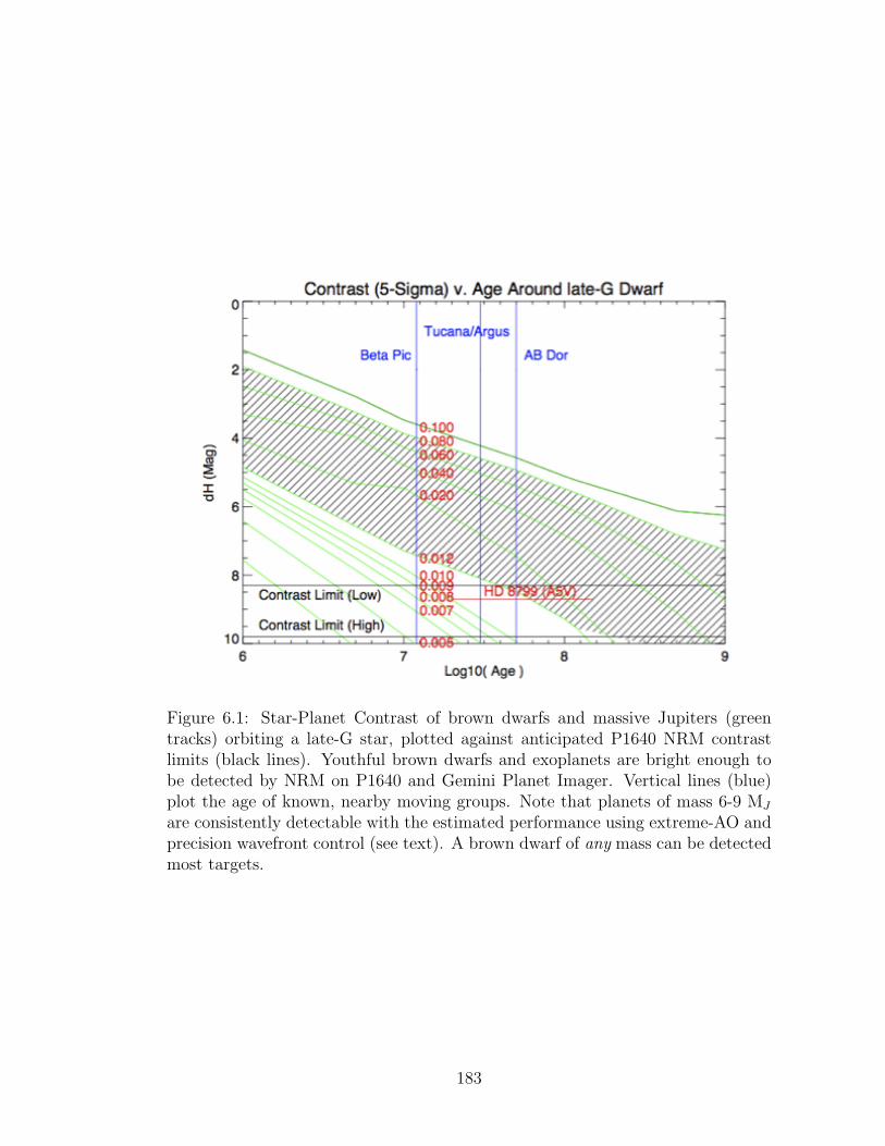
Figure 6.1: Star-Planet Contrast of brown dwarfs and massive Jupiters (greentracks) orbiting a late-G star, plotted against anticipated P1640 NRM contrastlimits (black lines). Youthful brown dwarfs and exoplanets are bright enough tobe detected by NRM on P1640 and Gemini Planet Imager. Vertical lines (blue)plot the age of known, nearby moving groups. Note that planets of mass 6-9 MJ
are consistently detectable with the estimated performance using extreme-AO andprecision wavefront control (see text). A brown dwarf of any mass can be detectedmost targets.
183
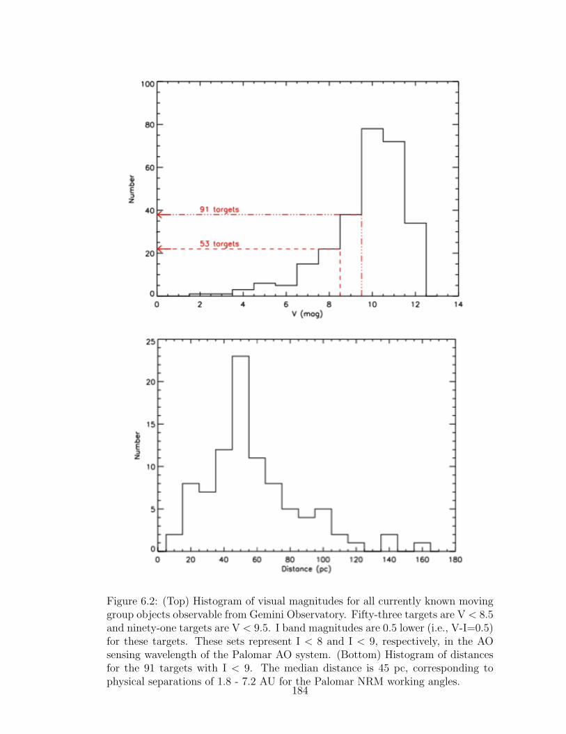
Figure 6.2: (Top) Histogram of visual magnitudes for all currently known movinggroup objects observable from Gemini Observatory. Fifty-three targets are V < 8.5and ninety-one targets are V < 9.5. I band magnitudes are 0.5 lower (i.e., V-I=0.5)for these targets. These sets represent I < 8 and I < 9, respectively, in the AOsensing wavelength of the Palomar AO system. (Bottom) Histogram of distancesfor the 91 targets with I < 9. The median distance is 45 pc, corresponding tophysical separations of 1.8 - 7.2 AU for the Palomar NRM working angles.
184
separations and testing models of their astrophysical evolution.
I presented results of a detection search for companions to sixteen nearby,
known brown dwarfs using NRM with LGSAO on the Palomar 200” Hale Tele-
scope. The four candidate brown dwarf companions detected with this survey,
if confirmed, these brown dwarfs make excellent candidates for dynamical mass
measurement. (Chapter 4)
I investigated the impact of small-scale wavefront errors (those smaller than a
sub-aperture) on NRM using a technique known as spatial filtering through calcula-
tion, simulation, and observational tests conducted with an optimized pinhole and
aperture mask in the PHARO instrument at the 200” Hale Telescope. I find that
spatially filtered NRM can increase observation contrasts by 10-25% on current
AO systems and by a factor of 2-4 on higher-order AO systems.
Completing this work required several new numerical and statistical methods
for using NRM with AO to detect faint companions. The improved analysis tools
allow for confident detection of faint targets by NRM, robust calculation of contrast
limits, and empirical averaging techniques that yield lower closure phase noise. I
also developed a formalism for detailing the impact of sub-aperture quasi-static
wavefront errors on closure phases that will be valuable for improving higher order
calibration techniques for NRM with exoplanet imaging instruments.
Combined, the evidence presented in this dissertation leads to the conclusion
that NRM with AO is rapidly developing into a fully mature high-contrast tech-
nique. With further attention and subsequent studies with more advanced instru-
mentation, the exoplanets resolved by NRM will contribute key scientific discov-
eries to the burgeoning population of directly imaged planetary systems.
185
APPENDIX A
PRIMER: IMAGING THROUGH A TURBULENT ATMOSPHERE
WITH ADAPTIVE OPTICS
A.1 The Point Spread Function
The image intensity pattern incident on the telescope detector, I(~θ), can be rep-
resented as the convolution of the object (or source) intensity distribution on the
sky, S(~θ), with the point spread function of the atmosphere and telescope, τ(~θ):
I(~θ) = S(~θ) ? τ(~θ), (A.1)
where the star, ?, denotes convolution. This representation is valid when the
object under consideration is small enough that its emitted light is perturbed by
essentially identical optical aberrations, i.e., isoplanatic. When this condition is
valid is dependent on the the quality of seeing but is typically on the order of a
few arcseconds in the infrared.
The source, located far enough to be considered at infinity, imparts a electric
field plane wave upon the telescope aperture (Ea) which is the Fourier Transform
of the electric field emitted by the source (Es).
Ea(~x) =
∫Es(~θ) exp(2πi~θ · ~x/λ)d~θ (A.2)
Throughout this text we will denote this form of the Fourier Transform by Ea(~x) =
F [Es(~θ)].
Equation A.1 can be derived directly by considering the truncation of the in-
coming wavefront at the telescope pupil. We represent the transmission of the
pupil by a two dimensional function, P (~x), valued zero where light is blocked and
186

one where light is fully transmitted. Apodized pupils can be represented by giving
the function a value between zero and one.
The electric field distribution incident upon the detector (Ed) is directly related
to the Fourier Transform of the wavefront incident on the telescope aperture. The
detector is located at the so-called image (or focal) plane, and measured in angular
units ~θ; the telescope aperture is in the pupil plane, and measured in physical units
(i.e., meters), ~x.
Ed = F [Ea(~x)P (~x)]
= Es(~θ) ? F [P (~x)]
Id(~θ) = < |Ed(~x)|2 >
= S(~θ) ? |F [P (~x)]|2. (A.3)
In the equations above, the brackets denote a time average over many cycles of the
emitted electric field. Inherent in this derivation is the assumption that the source
is spatially incoherent, i.e., < Es(~θ1)E∗s (~θ2) >= S(~θ)δ(~θ2 − ~θ1).
In analog to Equation A.1, the point spread function is
τ(~θ) = |F [P (~x)]|2. (A.4)
For an idealized telescope (i.e., a circular top-hat function of diameter D), this
leads to the familiar Airy function point spread function.
Atmospheric turbulence introduces perturbations to the wavefront incident on
the telescope aperture and imperfect optics further perturb the wavefront during
its propagation to the detector. To a good approximation, these errors can be
considered as pupil-plane phase errors; scintillation by the atmosphere produces
amplitude changes on the order of 10−4, optical errors impart phase errors in both
187
the pupil plane and image plane but can be approximated as only the former. Thus,
the wavefront is modified by aberrations of the form A(x) = eiφ(x), where φ(x) is
the phase error introduced across the pupil plane. If we treat the aberrations as a
modification to the pupil function, the distorted point spread function is
τ [~θ] = |F [eiφ(~x)P (~x)]|2. (A.5)
The structure of the wavefront aberrations drive the form of the short and
long exposure aberrated point spread function. While uncorrected atmospheric
turbulence perturbs the point spread function in an unknown way at every instant,
its long exposure average value is a well-determinable function of the aperture
and atmospheric seeing. On short times (defined by timescales shorter than the
timescale by which the wavefront aberrations, τ0), the phase aberrations can be
approximated as static; the resulting image is composed largely of the granular
structure of speckles. As the exposure extends over several coherence lengths,
many instances of speckles ultimately smear the image. Flux is displaced from
the core of the perfect point spread function core into a larger diffuse area. For
typical uncorrected atmospheric seeing in the infrared, the coherence time of the
atmosphere is tens of milliseconds and the long exposure image has a full width
half max of approximately one arc second.
Fourier Domain
Taking the Fourier Transform of the image in Equation A.3 yields
i(~f) =
∫P (~x+ ~f)P ∗(~x) < Ea(~x+ ~f)E∗a(~x) > d~x. (A.6)
The term < Ea(~x+ ~f)E∗a(~x) > is the spatial coherence function of the electric field
incident on the aperture or, alternatively, referred to as the (complex) visibility
188
V (~f) when normalized so that V (0) = 1. Importantly, the complex visibility is
fundamentally related to the source intensity distribution, a relationship known as
the van Cittert-Zernike theorem (Thompson, 2001):
V (~f) = < Ea(~x+ ~f)E∗a(~x) > / < |Ea(0)|2 > and (A.7)
V (~f) =
[∫S(~θ) exp(2πi~θ · ~f/λ) d~θ
]/
[∫S(~θ) d~θ
]. (A.8)
Likewise, the Fourier Transform of the image reduces to
i(~f) = V (~f) T (~f) with (A.9)
T (~f) =
∫d~x P (~x+ ~f)P ∗(~x)eiφ(~x+~f)−iφ(~x). (A.10)
where T (~f) is the optical transmission function, representing the amount by which
a given spatial frequency, ~f , is transmitted by the atmosphere and telescope.
This recasts the direct imaging problem as a challenge to obtain precision mea-
surements of the complex visibility. The complex visibility, by Equation A.8, is a
direct measure of one Fourier component the source brightness distribution.
A.2 Atmospheric Turbulence and Adaptive Optics
A.2.1 Kolmogorov Turbulence
Spatial Structure of Atmospheric Turbulence
The wavefront phase fluctuations imparted by the atmosphere arise because the
wavefront propagates through a large number of small index of refraction variations
of various physical sizes on its path to the telescope aperture. By the law of
189

large numbers, this aggregate deformation is Gaussian, and the variation of the
wavefront phase at any one point in space and time is a Gaussian random variable.
The wavefront variation has a spatial structure dependent on the mechanism which
drives the fluctuations, and this can most easily be facilitated by discussing the
phase structure function, Dφ(~r1, ~r2), describing the mean-squared phase variations
between two points in space separated by a distance vector, ~r = ~r1−~r2, at a given
instant in time.
Dφ(~r1, ~r2) =< [φ(~r1)− φ(~r2)]2 > . (A.11)
The brackets imply averaging over the spatial extent of the turbulence.
Turbulence arises by velocity fields mixing different layers of air in pressure
equilibrium, but with different temperatures, densities, and indices of refraction;
these small differences in local velocities move pockets of high and low temperature
(and density) around in a random fashion. Kolmogorov (1941) first studied the
spatial structure of these velocity differences. In principle, the structure function
varies at each point due to its local instantaneous conditions, but with a few
assumptions the problem is greatly simplified. If the atmosphere is assumed to
be homogenous, isotopic, and incompressible, a single structure function can be
applied to every point of origin and depends only on the total displacement between
two points, i.e, r = |~r1 − ~r2| and Dv(~r1, ~r2) = f(|~r1 − ~r2|) (Batchelor, 1953).
Furthermore, Kolmogorov showed that, for the spatial scales in which these
eddies more by turbulent flow, a scale generally ranging from millimeters to kilo-
meters for typical wind speeds (∼5 m/s), the structure function reduces to a single
power law function: D(r) = C2vr
2/3. The constant C2v is a measure of the energy
in the turbulence.
Tatarskii (1961) later related the random motions of these pockets of temper-
190
ature variation to index of refraction inhomogeneities, finding that the index of
refraction structure function also follows a 2/3 power law: Dn(r) = C2nr
2/3. Given
a measure of the turbulence strength, C2n, this equation completely describes the
statistical nature of index of refraction (and phase) fluctuations. The structure
constant C2n varies with broadly over seasons, as well as daily and hourly.
The structure constant also varies with height in the atmosphere, and the wave-
front propagates through many individual turbulence cells. The total deformation
of the wavefront is found by integrating over the depth of the atmosphere, leading
to the phase structure function, D(r) =< [φ(x+ r)− φ(x)]2 > expressed as:
Dφ(r) = 2.91 r5/3 sec(z)
(2π
λ
)2 ∫dh C2
n(h) (A.12)
= 6.88
(r
r0
)5/3
(A.13)
with
r0 =
[0.423 sec(z)
(2π
λ
)2 ∫ L
0
C2n(h)dh
]−3/5
. (A.14)
Thus the nature of atmospheric phase variation across an aperture reduces to
a fairly simple expression, i.e, phase variations are gaussian distributed at each
point with a variance which follows the structure function expression. Despite
the complex mechanisms driving atmospheric turbulence, its statistical nature can
be characterized by a single parameter, the Fried parameter r0, which is a func-
tion of the turbulence strength, zenith angle, cumulative path length through the
atmosphere, and wavelength.
191
Significance of the Fried Parameter, r0
While the Fried parameter has been introduced here as a matter of convenient
bookkeeping, the parameter naturally lends itself to a deeper significance. Indeed,
Fried (1966) introduced the parameter as the maximum diameter of an aperture
before atmospheric distortion seriously limits its resolving performance. That is,
the seeing-limited resolution of a large telescope obtained through an atmosphere
characterized by a Fried parameter, r0, is no better than the resolution of a diffrac-
tion limited telescope of diameter r0. Both circumstances lead to a point spread
function of full width at half max ∼ λ/r0.
In particular, despite the dependence of the Fried parameter on the turbulence
strength constant (and each layer of the atmosphere) and the zenith angle, an
estimate of r0 can be obtained by measuring the full-width half-max of a long-
exposure uncorrected image.
Furthermore, Noll (1976) showed that the wavefront variance averaged across
an aperture of size r0 is σ2 = 1.03rad2, or more generally σ2 = 1.03(D/r0)5/3 for
an aperture of diameter D. Two points separated by more than r0 are essentially
incoherent. This result leads to the adoption of a simple picture of turbulence as a
collection of cells of r0 with constant phase, but random phase between individual
cells.
From its definition in Equation A.14, r0 can be see to vary as a function of
λ6/5. With r0 ∼30 cm in H band (1.6µm), this scaling implies that even 5-10
meter class telescopes are diffraction limited in the mid-infrared (λ > 10µm).
Diffraction limited performance of adaptive optics systems is easier to achieve at
longer wavelengths and fewer actuators are necessary.
192
Turbulence in the Fourier Domain
Additionally, one can calculate the power spectral density of the structure function,
detailing the strength of phase fluctuations to a given spatial frequency. As we
will see in later sections, aperture masking interferometry measures specific spatial
frequencies of the incoming wavefront, and such, this description of turbulence is
in some ways more natural to this task. This calculation results in the Kolmogorov
Power Spectrum:
Φn(k) =0.023
r5/30
k−11/3. (A.15)
Thus, the phase variation across an aperture can be decomposed to indepen-
dent (Fourier) spatial frequencies. The phase of these spatial frequencies, in turn,
are subject to random Gaussian fluctuations with a variance which follows the Kol-
mogorov Power Spectrum. The steep negative slope of the Kolmogorov spectrum
implies that power preferentially resides in low-spatial frequency (i.e., large scale)
perturbations to the wavefront (Noll, 1976). Large scale wavefront errors result in
diffraction speckles in the image, indicating that speckles ought to determine the
structure of short exposure images and dominate the image noise.
Temporal Variation of the Wavefront
Turbulence is a time-varying phenomena, as local inhomogeneities are driven by
winds and eddies. The simplest model of this effect, the Taylor hypothesis of frozen
turbulence treats the atmosphere as a static, spatial phase structure that is blown
across the aperture by some wind with velocity, v. (If multiple levels contribute to
the total turbulence, the temporal behavior can still be treated by assuming the
turbulence weighted wind velocity.) Under this assumption, the temporal variation
193
of the phase over a time interval, τ , is equivalent to the spatial variation of the
phase over distance vτ .
Dφ,Taylor(δt = τ, δr = 0)⇐⇒ Dφ,Frozen(δt = 0, δr = vτ). (A.16)
Under these assumptions, the wavefront becomes decoherent over timescales of
τ0 = r0/v. With typical wind speeds on the order of 5-10 m/s, t0 ∼30-60 ms. By
its definition, τ0 also scales as λ6/5.
This timescale provides a natural length of time to separate long exposures
from short exposures. Short exposures, t << τ0, are perturbed, essentially, by
a single instantaneous realization of the atmosphere. In these circumstances, the
high spatial frequency information of the image is retained. This forms the basis
of speckle interferometry. Long exposures, alternatively, quickly lose high spatial
frequency information. The granular structure of speckles smooth away and the
halo forms.
A more in depth treatment of turbulence recognizes that the truncation of
turbulence cells at the aperture edge results in rapid fluctuation of the high spatial
frequencies as these cells are blown across the aperture edge. Greenwood (1976)
calculated that the characteristic frequency of turbulence variations to be
fg = 2.31λ−6/5
[sec(z)
∫ L
0
dh C2n(h) v5/3(h)
]3/5
. (A.17)
For the constant wind case, the Greenwood frequency can be approximated as
fg ≈ 0.43v
r0
≈ 0.431
τ0
. (A.18)
For typical observing the Greenwood frequency is tens of hertz. To effectively
reduce most of the phase fluctuations, adaptive optics systems must be capable of
correcting the wavefront at a rate much faster than this frequency.
194
A.3 Adaptive Optics
Adaptive optics systems function on the basis of phase conjugation, noting that
phase deformations can be corrected by reflecting the incoming wavefront off a de-
formed mirror in which the path length difference created along the mirror matches
the conjugate of the deformed wavefront. Sensing the wavefront distortions of the
incoming wavefront is often done by picking off a particular wavelength band of
the incoming flux that will not be used for science observations.
Typically, the pupil plane aperture is subdivided into a number of sub-apertures
by a wavefront sensor which utilizes a method for measuring the phase across each
sub-aperture. For instance, a Shack-Hartmann wavefront sensor uses a lenslet
array to focus each sub-aperture onto a CCD, and the displacement of the spots
from a reference position indicate the slope of the wavefront across each sub-
aperture. These wavefront slopes are then used to reconstruct the overall shape of
the wavefront.
The steep negative slope of the turbulence power spectrum (k−11/3) indicates
that the overwhelming power of the turbulence arises at large scales (low spatial
frequencies). Noll (1976) showed that ∼85% of the spatial variance of the phase
across an aperture arises from variations of the tip and tilt of the wavefront. These
wavefront errors do not degrade the overall structure of the instantaneous point
spread function but rather shift the image about on the science camera (giving rise
to an image wander in successive short exposures and smearing in long exposures).
For this reason, many adaptive optics systems implement an additional component
to control the translational motion of the image.
The deformable mirror receives the measurements from the wavefront sensor
195
and implements phase conjugation. A zonal approach of phase conjugation posi-
tions each actuator to minimize a least squared fit between the deformable mirror
surface and the turbulent wavefront. Or alternatively, a modal approach decom-
poses the wavefront into Zernike modes and introduces conjugate modes into the
deformable mirror to remove some subset of Zernike modes from the turbulent
wavefront (see, for example, Nakajima & Haniff (1993)).
Current generation adaptive optics systems dramatically reduce the effects of
atmospheric turbulence and alter the spatial and temporal power spectrum of the
wavefront phase. The characteristics of the adaptive optics corrected wavefront
and the limitations to correction are discussed here.
The finite spacing of the actuators limit the smallest wavefront features which
can be corrected (i.e., the highest frequency variation that happens within the
scale of the actuator size). This limits the field of view which can be corrected by
adaptive optics. The outer field of view of an image is formed by the high-spatial
frequency content of the wavefront; since the adaptive optics system cannot correct
the wavefront on scales smaller than r < ra, where ra is the actuator spacing, the
adaptive optics cannot correct the field of view beyond λ/ra. Beyond this outer
control radius, the region is essentially identical to the seeing limited case.
The length of time required for the wavefront sensor to gather enough photons
to measure the wavefront and the finite response lag between measurement and
implementation both introduce an error between the atmospheric wavefront and
the phase conjugation. Because the wavefront sensor is photon limited, the rate
at which the adaptive optics control system can be run is a function of the guide
star brightness.
196
In addition to atmospheric turbulence, imperfections of the optics introduce
wavefront errors as well. Wavefront optical elements which occur before the wave-
front sensor (for instance, the primary mirror) can be corrected by the adaptive
optics system, up to the limitations of the actuator spacing. Smaller scale (higher
frequency) components remain in the wavefront. Optical elements which occur
after the wavefront sensor cannot be be corrected. These non-common path er-
rors have become a focus of the high-contrast imaging community, as these errors
generally set the ultimate limitation of contrast on can achieve with a system.
The performance of current adaptive optics systems are primarily characterized
in terms of the residual phase variance across the telescope aperture. This phase
variance can be reasonably well estimated by summing the individual error terms
described above. The estimated performance of a generic adaptive optics system is
given below, along with the specific performance of the Palomar Adaptive Optics
systems with the PHARO infrared imager on the Hale 200” Telescope (Troy et al.,
2000).
Adaptive Optics Spatial Errors
The finite spacing of the actuators (ra, Na actuators total) limit the smallest fea-
tures of the wavefront which can be corrected. Zonal methods aim to minimize
the overall wavefront variance over the aperture after correction; Model methods
decompose the wavefront structure into a set of linearly independent components
(usually Zernike modes) and configure the actuators to remove the lowest modes.
Both methods produce similar correction. It is generally assumed that an adap-
tive optics system can remove spatial wavefront errors on scales larger than 2ra
(frequencies lower than λ/2ra), or alternatively the Na lowest Zernike mode.s
197
The residual atmospheric wavefront error after zonal correcting scales are
σ2fit = κ
(rsr0
)5/3
, (A.19)
where κ depends on the various basis functions and influence properties of the
actuators. For PALAO, κ = 0.28. Noll (1976) developed an approximate relation
for the residual wavefront error after modal correction:
σ2fit = 0.2944N
√3/2
a
(D
r0
)5/3
. (A.20)
The similarity of the two equations can be seen when ra ∼ D/√Na is substituted
into the former.
The PALAO system at Palomar utilizes Na = 241 actuators, with an actuator
spacing of ra = 31.2 cm. For typical H band (1.6 µm) seeing of 30 cm, this yields
atmospheric residual error of σfit ∼ 142 nm. The residual wavefront error due to
optical imperfections depends on the telescope and instrument and are estimated
to be ∼100 nm.
Adaptive Optics Temporal Errors
Greenwood (1979) showed the residual phase errors which result from the finite
rate at which the adaptive optics system measure and apply correction is
σ2temp = κt
(fgfs
)5/3
, (A.21)
where, fg is the Greenwood frequency (Eq. A.18) and fs is the control loop fre-
quency. The constant κt depends on the servo algorithm; it is approximately 1 for
the PALAO system. Note that these errors arise even if the adaptive optics system
were able to perfectly conjugate the atmospheric wavefront, and instead result due
198
to the lag between the wavefront sensor measurement and implementation of the
wavefront conjugate on the mirror.
The dynamical control loop of the adaptive optics system will also alter the tem-
poral power spectrum of the wavefront phase, and with it the temporal structure
function. Indeed, the Taylor hypothesis now only applies to those time intervals
shorter than the control loop period, ts = 1/fs. For time intervals longer than the
servo period the wavefront at a specific point can be regarded as uncorrelated, and
the structure function asymptotes to the Greenwood time-delay residuals.
DAO(t, δr = 0) = 6.88 (fg t)5/3, t . 2ts (A.22)
= 2σ2temp, t & 2ts (A.23)
and < φ(t+ δt)φ∗(t) >= 0 when t & 2ts.
Figure A.1 shows the temporal power spectrum of the residuals obtained with
the PALAO high-order deformable mirror during observations of a bright star.
The ”open loop” residuals show the temporal power spectrum of the atmospheric
turbulence; a clear t−5/3 power spectrum can be seen, consistent with the Kol-
mogorov model and the Taylor hypothesis. Operating with ”closed loop” (i.e., the
deformable mirror control loop activated), the adaptive optics system effectively
removed turbulence power at frequencies slower than fs ∼ 15Hz (timescales longer
than ts ∼ 65 msec). From these results, one can conclude that the corrected
wavefront decorrelates after 65 msec.
The PALAO system also uses an additional mirror to stabilize the image, i.e.
correct for tip-tilt wavefront errors. The finite time of implementation introduces
199
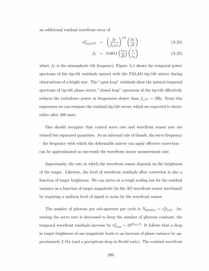
an additional residual wavefront error of
σ2temp,TT =
(fTfs,TT
)1/6(λTD
)(A.24)
fT ∼ 0.0811(r0
D
)( v
r0
)(A.25)
where fT is the atmospheric tilt frequency. Figure A.1 shows the temporal power
spectrum of the tip-tilt residuals opened with the PALAO tip/tilt mirror during
observations of a bright star. The ”open loop” residuals show the natural temporal
spectrum of tip-tilt phase errors; ”closed loop” operation of the tip-tilt effectively
reduces the turbulence power at frequencies slower than fs,TT ∼ 5Hz. From this
expression we can estimate the residual tip/tilt errors, which are expected to decor-
relate after 200 msec.
One should recognize that control servo rate and wavefront sensor rate are
related but separated quantities. As an informal rule of thumb, the servo frequency
– the frequency with which the deformable mirror can apply effective correction –
can be approximated as one-tenth the wavefront sensor measurement rate.
Importantly, the rate at which the wavefront sensor depends on the brightness
of the target. Likewise, the level of wavefront residuals after correction is also a
function of target brightness. We can arrive at a rough scaling law for the residual
variance as a function of target magnitude (in the AO wavefront sensor waveband)
by requiring a uniform level of signal to noise by the wavefront sensor.
The number of photons per sub-aperture per cycle is Nphotons ∼ r2atwfs. As-
suming the servo rate is decreased to keep the number of photons constant, the
temporal wavefront residuals increase by σ2temp ∼ 10MAO/3. It follows that a drop
in target brightness of one magnitude leads to an increase of phase variance by ap-
proximately 2.15x (and a precipitous drop in Strehl ratio). The residual wavefront
200
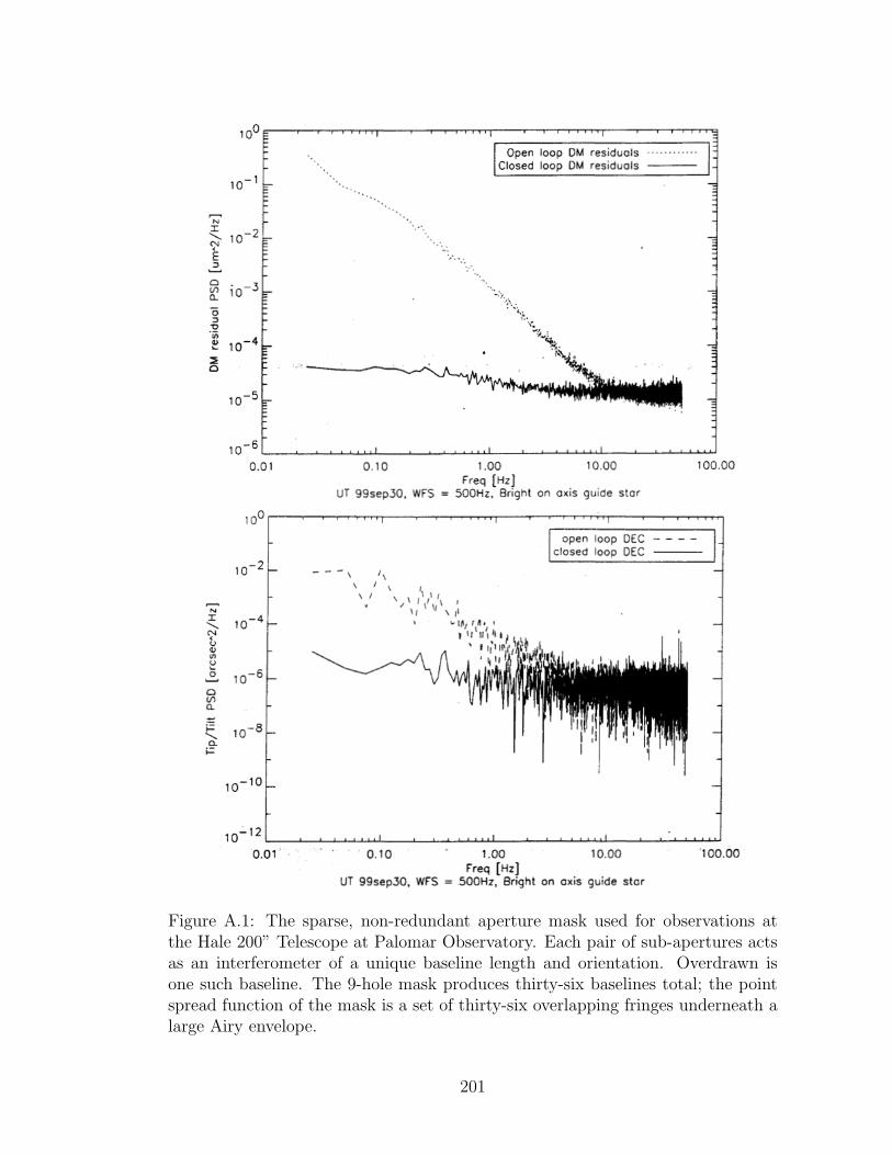
Figure A.1: The sparse, non-redundant aperture mask used for observations atthe Hale 200” Telescope at Palomar Observatory. Each pair of sub-apertures actsas an interferometer of a unique baseline length and orientation. Overdrawn isone such baseline. The 9-hole mask produces thirty-six baselines total; the pointspread function of the mask is a set of thirty-six overlapping fringes underneath alarge Airy envelope.
201
tip-tilt errors vary less dramatically due to the lower order exponent in Equation
A.24.
Given typical wind speeds at Palomar of about 5 m/s and servo control fre-
quencies of fs ∼15 Hz and fs,tt ∼5 Hz (valid for bright stars), temporal residual
errors are σtemp ∼140 nm and σtemp,TT .
Adaptive Optics Structure Function
These results motivate the adaptive optics corrected structure function given by
Greenwood (1979):
DAO(r) = 6.88(r/r0)5/3, r . rs (A.26)
= 2σ2fit, r & rs (A.27)
with the implicit conclusion that wavefront residuals are not spatially correlated
at separations larger than rs: < φ(~x+ ~r)φ∗(~x) >= 0 when |~r| & rs.
Likewise, adaptive optics provides a high pass filter to the Kolmogorov Power
Spectrum, effectively eliminating power at spatial frequencies below kAO < 2π/2rs.
202
BIBLIOGRAPHY
Alexander, D. R. & Ferguson, J. W. 1994, Astrophysical Journal, 437, 879
Allard, F., Guillot, T., Ludwig, H.-G., Hauschildt, P. H., Schweitzer, A., Alexan-
der, D. R., & Ferguson, J. W. 2003, Brown Dwarfs, 211, 325
Allard, F., Hauschildt, P. H., Alexander, D. R., Ferguson, J. W., & Tamanai, A.
2000, From Giant Planets to Cool Stars, 212, 127, iSBN: 1-58381-041-2
Allen, P. 2007, The Astrophysical Journal
Allen, P. R., Koerner, D. W., Reid, I. N., & Trilling, D. E. 2005, The Astrophysical
Journal, 625, 385
Allen, P. R., Trilling, D. E., Koerner, D. W., & Reid, I. N. 2003, The Astrophysical
Journal, 595, 1222
Baldwin, J. E., Haniff, C. A., Mackay, C. D., & Warner, P. J. 1986, Nature (ISSN
0028-0836), 320, 595
Baraffe, I., Chabrier, G., Allard, F., & Hauschildt, P. 1998, arXiv, astro-ph
Baraffe, I., Chabrier, G., Barman, T. S., Allard, F., & Hauschildt, P. H. 2003,
Astronomy and Astrophysics, 402, 701
Basri, G. & Reiners, A. 2006, The Astronomical Journal, 132, 663
Batchelor, G. K. 1953, The Theory of Homogeneous Turbulence
Beichman, C. A., Krist, J., Trauger, J. T., Greene, T. P., Oppenheimer, B., Sivara-
makrishnan, A., Doyon, R., Boccaletti, A., Barman, T. S., & Rieke, M. 2010,
arXiv, astro-ph.IM
203
Bernat, D., Bouchez, A. H., Ireland, M., Tuthill, P., Martinache, F., Angione, J.,
Burruss, R. S., Cromer, J. L., Dekany, R. G., Guiwits, S. R., Henning, J. R.,
Hickey, J., Kibblewhite, E., McKenna, D. L., Moore, A. M., Petrie, H. L.,
Roberts, J., Shelton, J. C., Thicksten, R. P., Trinh, T., Tripathi, R., Troy, M.,
Truong, T., Velur, V., & Lloyd, J. P. 2010, The Astrophysical Journal, 715, 724
Beuzit, J.-L., Feldt, M., Dohlen, K., Mouillet, D., Puget, P., Antichi, J., Baruffolo,
A., Baudoz, P., Berton, A., Boccaletti, A., Carbillet, M., Charton, J., Claudi,
R., Downing, M., Feautrier, P., Fedrigo, E., Fusco, T., Gratton, R., Hubin, N.,
Kasper, M., Langlois, M., Moutou, C., Mugnier, L., Pragt, J., Rabou, P., Saisse,
M., Schmid, H. M., Stadler, E., Turrato, M., Udry, S., Waters, R., & Wildi, F.
2006, The Messenger, 125, 29
Bloemhof, E., Marsh, K., Dekany, R., & Troy. . . , M. 2000, spie.org
Bloemhof, E. E., Dekany, R. G., Troy, M., & Oppenheimer, B. R. 2001, The
Astrophysical Journal, 558, L71
Boss, A. P. 2001, The Astrophysical Journal, 551, L167
Bouy, H., Brandner, W., Martın, E., & Delfosse, X. 2003, The Astronomical Jour-
nal
Burgasser, A. J., Liu, M. C., Ireland, M. J., Cruz, K. L., & Dupuy, T. J. 2008, The
Astrophysical Journal, 681, 579, (c) 2008: The American Astronomical Society
Burgasser, A. J., Reid, I. N., Siegler, N., Close, L., Allen, P., Lowrance, P., &
Gizis, J. 2007, Protostars and Planets V, 427
Burrows, A., Heng, K., & Nampaisarn, T. 2011, The Astrophysical Journal, 736,
47
204
Burrows, A., Hubbard, W. B., Lunine, J. I., Guillot, M. M. T., Saumon, D., &
Freedman, R. S. 1997, arXiv, astro-ph
Burrows, A., Hubbard, W. B., Lunine, J. I., & Liebert, J. 2001, arXiv, astro-ph
Burrows, A. & Sharp, C. M. 1999, The Astrophysical Journal, 512, 843
Burrows, A., Sudarsky, D., & Hubeny, I. 2005, arXiv, astro-ph
—. 2006, The Astrophysical Journal, 640, 1063
Chabrier, G., Baraffe, I., Allard, F., & Hauschildt, P. 2000, The Astrophysical
Journal, 542, 464, (c) 2000: The American Astronomical Society
Chappelle, R. J., Pinfield, D. J., Steele, I. A., Dobbie, P. D., & Magazzu, A. 2005,
Monthly Notices of the Royal Astronomical Society, 361, 1323
Close, L. M., Siegler, N., Freed, M., & Biller, B. 2003, The Astrophysical Journal,
587, 407
Cornwell, T. J. 1989, Science (ISSN 0036-8075), 245, 263
Crepp, J. R., Pueyo, L., Brenner, D., Oppenheimer, B. R., Zimmerman, N., Hink-
ley, S., Parry, I., King, D., Vasisht, G., Beichman, C., Hillenbrand, L., Dekany,
R., Shao, M., Burruss, R., Jr., L. C. R., Bouchez, A., Roberts, J., & Soummer,
R. 2010, arXiv, astro-ph.IM, accepted to ApJ
Cruz, K. L., Reid, I. N., Liebert, J., Kirkpatrick, J. D., & Lowrance, P. J. 2003,
The Astronomical Journal, 126, 2421
Dahn, C. C., Harris, H. C., Vrba, F. J., Guetter, H. H., Canzian, B., Henden,
A. A., Levine, S. E., Luginbuhl, C. B., Monet, A. K. B., Monet, D. G., Pier,
J. R., Stone, R. C., Walker, R. L., Burgasser, A. J., Gizis, J. E., Kirkpatrick,
J. D., Liebert, J., & Reid, I. N. 2002, The Astronomical Journal, 124, 1170
205
Dekany, R., Bouchez, A., Roberts, J., Troy, M., Kibblewhite, E., Oppenheimer,
B., Moore, A., Shelton, C., Smith, R., Trinh, T., & Velur, V. 2007, Proceedings
of the Advanced Maui Optical and Space Surveillance Technologies Conference,
64
du Foresto, V. C., Ridgway, S., & Mariotti, J.-M. 1997, A & A Supplement series,
121, 379
Dupuy, T., Liu, M., Bowler, B., Cushing, M., Helling, C., Witte, S., & Hauschildt,
P. 2010, arXiv, astro-ph.SR, 53 pages, 12 figures, accepted to ApJ
Dupuy, T. J., Liu, M. C., & Ireland, M. J. 2009, The Astrophysical Journal, 699,
168, apJ, in press
—. 2011, eprint arXiv, 1103, 5747
Fabrycky, D. C. & Murray-Clay, R. A. 2010, The Astrophysical Journal, 710, 1408
Ferrari, A. 2007, The Astrophysical Journal, 657, 1201
Fortney, J. J., Marley, M. S., Saumon, D., & Lodders, K. 2008, The Astrophysical
Journal, 683, 1104
Fried, D. 1966, JOSA
Glindemann, A., Lane, R. G., & Dainty, J. C. 1993, Journal of Modern Optics, 40,
2381
Golimowski, D., Leggett, S., & Marley. . . , M. 2004, The Astronomical . . .
Greenwood, D. 1976, Atmosphere
Greenwood, D. P. 1979, Journal of the Optical Society of America, 69, 549
Grossman, L. 1972, Geochimica et Cosmochimica Acta
206
Gull, S. F. & Skilling, J. 1984, Indirect Imaging: Measurement and Processing for
Indirect Imaging. Proceedings of an International Symposium held in Sydney,
267, iSBN: 0-521-26282-8
Haniff, C. A., Mackay, C. D., Titterington, D. J., Sivia, D., & Baldwin, J. E. 1987,
Nature (ISSN 0028-0836), 328, 694
Hayashi, C. & Nakano, T. 1963, Progress of Theoretical Physics, 30, 460
Hayward, T. L., Brandl, B., Pirger, B., Blacken, C., Gull, G. E., Schoenwald, J., &
Houck, J. R. 2001, The Publications of the Astronomical Society of the Pacific,
113, 105, (c) 2001: The Astronomical Society of the Pacific
Henry, T. J. & McCarthy, D. W. 1993, Astronomical Journal (ISSN 0004-6256),
106, 773
Hinkley, S. 2009, ProQuest Dissertations And Theses; Thesis (Ph.D.)–Columbia
University, 226
Hinkley, S., Oppenheimer, B. R., Brenner, D., Zimmerman, N., Roberts, L. C.,
Parry, I. R., Soummer, R., Sivaramakrishnan, A., Simon, M., Perrin, M. D.,
King, D. L., Lloyd, J. P., Bouchez, A., Roberts, J. E., Dekany, R., Beichman, C.,
Hillenbrand, L., Burruss, R., Shao, M., & Vasisht, G. 2010, The Astrophysical
Journal, 712, 421
Hinkley, S., Oppenheimer, B. R., Soummer, R., Brenner, D., Graham, J. R., Perrin,
M. D., Sivaramakrishnan, A., Lloyd, J. P., Roberts, L. C., & Kuhn, J. 2009, The
Astrophysical Journal, 701, 804
Hinkley, S., Oppenheimer, B. R., Soummer, R., Sivaramakrishnan, A., Roberts,
L. C., Kuhn, J., Makidon, R. B., Perrin, M. D., Lloyd, J. P., Kratter, K., &
Brenner, D. 2007, The Astrophysical Journal, 654, 633
207
Hinkley, S., Oppenheimer, B. R., Zimmerman, N., Brenner, D., Parry, I. R., Crepp,
J. R., Vasisht, G., Ligon, E., King, D., Soummer, R., Sivaramakrishnan, A., Be-
ichman, C., Shao, M., Roberts, L. C., Bouchez, A., Dekany, R., Pueyo, L.,
Roberts, J. E., Lockhart, T., Zhai, C., Shelton, C., & Burruss, R. 2011, Publi-
cations of the Astronomical Society of the Pacific, 123, 74
Hogbom, J. A. 1974, Astronomy and Astrophysics Supplement, 15, 417, a&AA
ID. AAA011.033.031
Ida, S. & Lin, D. N. C. 2004, The Astrophysical Journal, 616, 567, (c) 2004: The
American Astronomical Society
Ireland, M. J., Kraus, A., Martinache, F., Lloyd, J. P., & Tuthill, P. G. 2008, The
Astrophysical Journal, 678, 463, 10 pages, 6 figures, accepted for ApJ
Jeffries, R. D. & Maxted, P. F. L. 2005, Protostars and Planets V, 8154
Jennison, R. C. 1958, Monthly Notices of the Royal Astronomical Society, 118, 276
Jones, H. R. A. 1997, The Astrophysical Journal Letters
Keen, J., Buscher, D., & Warner, P. 2001, Arxiv preprint astro-ph
Kirkpatrick, J. 1992, adsabs.harvard.edu
Kirkpatrick, J. D., Reid, I. N., Liebert, J., Cutri, R. M., Nelson, B., Beichman,
C. A., Dahn, C. C., Monet, D. G., Gizis, J. E., & Skrutskie, M. F. 1999, The
Astrophysical Journal, 519, 802
Knapp, G., Leggett, S., & Fan. . . , X. 2004, The Astronomical . . .
Kolmogorov, A. 1941, Dokl. Akad. Nauk SSSR, 30, 301
208
Konopacky, Q. M., Ghez, A. M., Barman, T. S., Rice, E. L., Bailey, J. I., White,
R. J., McLean, I. S., & Duchene, G. 2010, The Astrophysical Journal, 711, 1087
Kraus, A., Covey, K., Liu, M., Metchev, S., White, R., Prato, L., Lin, D., &
Marley, M. 2009, Astro2010: The Astronomy and Astrophysics Decadal Survey,
2010, 163
Kraus, A., Ireland, M., Martinache, F., & Lloyd, J. 2008, The Astrophysical Jour-
nal
Kraus, A. L., Ireland, M. J., Martinache, F., & Hillenbrand, L. A. 2011, The
Astrophysical Journal, 731, 8
Kulkarni, S. 1989, The Astronomical Journal
Kumar, S. S. 1963, Astrophysical Journal, 137, 1121
Lafreniere, D., Marois, C., Doyon, R., Nadeau, D., & Artigau, E. 2007, The As-
trophysical Journal, 660, 770
Lane, B. F., Osorio, M. R. Z., Britton, M. C., Martin, E. L., & Kulkarni, S. R.
2001, arXiv, astro-ph
Lane, R. G., Glindemann, A., & Dainty, J. C. 1992, Waves in Random Media, 2,
209
Leggett, S. K., Allard, F., & Hauschildt, P. H. 1998, The Astrophysical Journal,
509, 836
Lenzen, R., Close, L., Brandner, W., Biller, B., & Hartung, M. 2004, Ground-
based Instrumentation for Astronomy. Edited by Alan F. M. Moorwood and Iye
Masanori. Proceedings of the SPIE, 5492, 970
209
Linfield, R. P., Colavita, M. M., & Lane, B. F. 2001, The Astrophysical Journal,
554, 505
Liu, M. C., Dupuy, T. J., & Ireland, M. J. 2008, The Astrophysical Journal, 689,
436, apJ, in press. Typo in Eqn. 6 corrected in v2
Lloyd, J. P., Martinache, F., Ireland, M. J., Monnier, J. D., Pravdo, S. H., Shaklan,
S. B., & Tuthill, P. G. 2006, The Astrophysical Journal, 650, L131
Lohmann, A. W., Weigelt, G., & Wirnitzer, B. 1983, Applied Optics (ISSN 0003-
6935), 22, 4028
Lunine, J., Hubbard, W., & Burrows. . . , A. 1989, The Astrophysical . . .
Macintosh, B., Poyneer, L., Sivaramakrishnan, A., & Marois, C. 2005, Astronom-
ical Adaptive Optics Systems and Applications II. Edited by Tyson, 5903, 170
Macintosh, B. A., Graham, J. R., Palmer, D. W., Doyon, R., Dunn, J., Gavel,
D. T., Larkin, J., Oppenheimer, B., Saddlemyer, L., Sivaramakrishnan, A.,
Wallace, J. K., Bauman, B., Erickson, D. A., Marois, C., Poyneer, L. A., &
Soummer, R. 2008, Adaptive Optics Systems. Edited by Hubin, 7015, 31
Marcy, G., Butler, R. P., Fischer, D., Vogt, S., Wright, J. T., Tinney, C. G., &
Jones, H. R. A. 2005, Progress of Theoretical Physics Supplement, 158, 24
Marley, M. 2007, Proceedings of the conference In the Spirit of Bernard Lyot: The
Direct Detection of Planets and Circumstellar Disks in the 21st Century. June
04 - 08, 19
Marley, M., Saumon, D., Guillot, T., & Freedman. . . , R. 1996, Science
210

Marois, C., Doyon, R., Racine, R., Nadeau, D., Lafreniere, D., Vallee, P., Riopel,
M., & Macintosh, B. 2005, Journal of the Royal Astronomical Society of Canada,
99, 130
Marois, C., Lafreniere, D., Doyon, R., Macintosh, B., & Nadeau, D. 2006, The
Astrophysical Journal, 641, 556
Marois, C., Macintosh, B., Barman, T., Zuckerman, B., Song, I., Patience, J.,
Lafreniere, D., & Doyon, R. 2008, Science, 322, 1348
Marois, C., Zuckerman, B., & Konopacky. . . , Q. 2010, Nature
Martinache, F., Lloyd, J. P., Ireland, M. J., Yamada, R. S., & Tuthill, P. G. 2007,
The Astrophysical Journal, 661, 496, 7 pages, 5 figures. Accepted for ApJ
Martinache, F., Rojas-Ayala, B., Ireland, M. J., Lloyd, J. P., & Tuthill, P. G. 2009,
The Astrophysical Journal, 695, 1183, 9 pages, 8 figures. Submitted to ApJ
Mayor, M. 1995, Nature
Metchev, S. A., Hillenbrand, L. A., & White, R. J. 2003, The Astrophysical Jour-
nal, 582, 1102
Monnier, J. 2000, Principles of Long Baseline Stellar Interferometry
—. 2003, Reports on Progress in Physics
Morgan, W. W., Keenan, P. C., & Kellman, E. 1943, Chicago, 6., lCCN: 43-2093
(BKS1); CALL NUMBER: QB881 .M6
Nakajima, T. 1988, JOSA A
—. 1994, Astrophysical Journal, 425, 348
Nakajima, T. & Haniff, C. A. 1993, Astronomical Society of the Pacific, 105, 509
211

Nakajima, T., Kulkarni, S. R., Gorham, P. W., Ghez, A. M., Neugebauer, G., Oke,
J. B., Prince, T. A., & Readhead, A. C. S. 1989, Astronomical Journal (ISSN
0004-6256), 97, 1510
Nakajima, T., Oppenheimer, B. R., Kulkarni, S. R., Golimowski, D. A., Matthews,
K., & Durrance, S. T. 1995, Nature, 378, 463
Noll, R. J. 1976, Optical Society of America, 66, 207
Oppenheimer, B. R., Kulkarni, S. R., Matthews, K., & Nakajima, T. 1995, Science,
270, 1478
Oppenheimer, B. R., Kulkarni, S. R., Matthews, K., & van Kerkwijk, M. H. 1998,
Astrophysical Journal v.502, 502, 932
Osorio, M. R. Z., Lane, B. F., Pavlenko, Y., Martın, E. L., Britton, M., & Kulka-
rni, S. R. 2004, The Astrophysical Journal, 615, 958, (c) 2004: The American
Astronomical Society
Pinfield, D., Dobbie, P., Jameson, R., & Steele, I. 2003, Monthly Notice of the
Royal Astronomical Society
Poyneer, L. & Macintosh, B. 2004, Journal of the Optical Society of America A
Pravdo, S. H., Shaklan, S. B., & Lloyd, J. 2005, arXiv, astro-ph
Pravdo, S. H., Shaklan, S. B., Wiktorowicz, S. J., Kulkarni, S., Lloyd, J. P.,
Martinache, F., Tuthill, P. G., & Ireland, M. J. 2006, The Astrophysical Journal,
649, 389
Racine, R., Walker, G., Nadeau, D., Doyon, R., & Marois, C. 1999, Publications
of the Astronomical Society of the Pacific
212
Raymond, S. N., Barnes, R., Veras, D., Armitage, P. J., Gorelick, N., & Greenberg,
R. 2009, The Astrophysical Journal Letters, 696, L98
Readhead, A., Nakajima, T., & Pearson, T. 1988, Astronomical Journal (ISSN
0004-6256)
Rebolo, R., Martin, E. L., & Magazzu, A. 1992, Astrophysical Journal, 389, L83
Reid, I. N., Gizis, J. E., Kirkpatrick, J. D., & Koerner, D. W. 2001, The Astro-
nomical Journal, 121, 489, 38 pages, 11 figures; accepted for AJ
Reid, I. N., Lewitus, E., Allen, P. R., Cruz, K. L., & Burgasser, A. J. 2006, The
Astronomical Journal, 132, 891
Reipurth, B., Jewitt, D., & Keil, K. 2007, Protostars and Planets V
Roberts, J. E., Bouchez, A. H., Angione, J., Burruss, R. S., Cromer, J. L., Dekany,
R. G., Guiwits, S. R., Henning, J. R., Hickey, J., Kibblewhite, E., McKenna,
D. L., Moore, A. M., Petrie, H. L., Shelton, J. C., Thicksten, R. P., Trinh, T.,
Tripathi, R., Troy, M., Truong, T., & Velur, V. 2008, Adaptive Optics Systems.
Edited by Hubin, 7015, 74
Roddier, F. 1986, Optics Communications, 60, 145
Schlieder, J. & Lepine, S. 2010, The Astronomical Journal
Serabyn, E., Wallace, J. K., Troy, M., Mennesson, B., Haguenauer, P., Gappinger,
R. O., & Bloemhof, E. E. 2006, Advances in Adaptive Optics II. Edited by
Ellerbroek, 6272, 91
Shaklan, S. B. & Roddier, F. 1987, Applied Optics (ISSN 0003-6935), 26, 2159
Sivaramakrishnan, A., Koresko, C. D., Makidon, R. B., Berkefeld, T., & Kuchner,
M. J. 2001, arXiv, astro-ph, to appear in ApJ, May 2001 (28 pages, 10 figs)
213
Sivaramakrishnan, A., Lloyd, J. P., Hodge, P. E., & Macintosh, B. A. 2003, arXiv,
astro-ph, accepted to ApJL
Stassun, K. G., Mathieu, R. D., & Valenti, J. A. 2006, Nature, 440, 311
Stevenson, D. 1986, Astrophysics of Brown Dwarfs
Tatarskii, V. I. 1961
Tatulli, E., Blind, N., Berger, J. P., Chelli, A., & Malbet, F. 2010, arXiv, astro-
ph.IM
Torres, C. A. O., Quast, G. R., da Silva, L., de La Reza, R., Melo, C. H. F., &
Sterzik, M. 2006, Astronomy and Astrophysics, 460, 695
Troy, M., Dekany, R., Brack, G., Shi, F., & Oppenheimer. . . , B. 2000, trs-
new.jpl.nasa.gov
Tsuji, T. 1995, Laboratory and Astronomical High Resolution . . .
Tuthill, P., Lloyd, J., Ireland, M., Martinache, F., Monnier, J., Woodruff, H., ten
Brummelaar, T., Turner, N., & Townes, C. 2006, Advances in Adaptive Optics
II. Edited by Ellerbroek, 6272, 103
Tuthill, P. G., Monnier, J. D., Danchi, W. C., Wishnow, E. H., & Haniff, C. A.
2000, The Publications of the Astronomical Society of the Pacific, 112, 555, (c)
2000: The Astronomical Society of the Pacific
Veras, D., Crepp, J. R., & Ford, E. B. 2009, The Astrophysical Journal, 696, 1600
Weigelt, G. P. 1977, Optics Communications, 21, 55, a&AA ID. AAA020.031.281
Wildi, F., Brusa, G., Lloyd-Hart, M., & Close. . . , L. 2003, Proceedings of . . .
Wizinowich, P. 2006, Proceedings of SPIE
214
Ziad, A., Schock, M., Chanan, G. A., Troy, M., Dekany, R., Lane, B. F., Borgnino,
J., & Martin, F. 2004, Applied Optics, 43, 2316
Zimmerman, N., Oppenheimer, B. R., Hinkley, S., Brenner, D., Parry, I. R.,
Sivaramakrishnan, A., Hillenbrand, L., Beichman, C., Crepp, J. R., Vasisht,
G., Roberts, L. C., Burruss, R., King, D. L., Soummer, R., Dekany, R., Shao,
M., Bouchez, A., Roberts, J. E., & Hunt, S. 2010, The Astrophysical Journal,
709, 733
Zimmerman, N., Sivaramakrishnan, A., Bernat, D., & et al. 2011, in preparation
Zuckerman, B. 2004, Annu. Rev. Astron. Astrophys.
215
Recommended