MEMORANDUM
UNITED STATES ENVIRONMENTAL PROTECTION AGENCY
RESEARCH TRIANGLE PARK, NC 27711
AUG 0 7 2012 OFFICE OF
AIR QUALITY PLANNING AND STANDARDS
SUBJECT: Guidance on Removing Stage II Gasoline Refueling Vapor Recovery Programs
FROM:
from State Implementation Plans il:. ~
TO: Regional Air Division Directors
The purpose of this memorandum is to distribute a guidance document titled "Guidance on Removing Stage II Gasoline Vapor Control Programs from State Implementation Plans and Assessing Comparable Measures" (EPA-457/B12-001, August 07, 2012). Effective May 16, 2012, the Environmental Protection Agency has used its authority under Clean Air Act (CAA) section 202(a)(6) to waive certain statutory requirements for states to implement Stage II gasoline vapor recovery at gasoline dispensing facilities in all Serious, Severe, and Extreme ozone nonattainrnent areas. Accordingly, states implementing Stage II programs under CAA section 182(b )(3) are now legally able to phase out those programs if doing so does not interfere with attaining or maintaining the ozone standards. This guidance provides information and tools states can use to develop a Stage II program phase-out plan and an accompanying state implementation plan revision request.
States in the ozone transport region (OTR) also have a statutory obligation to implement Stage II vapor recovery programs or "comparable measures." The EPA does not have statutory authority to waive this requirement. However, this document contains new guidance on how OTR states can phase out Stage II control programs in a manner consistent with the CAA section 184(b )(2) comparable measures requirement.
Please distribute this guidance to your respective state and local air agencies. For questions on this guidance, please contact Mr. H. Lynn Dail, (919) 541-2363, [email protected].
Attachment
cc: Margo Oge, OTAQ Anna Wood, OAQPS Richard Wayland, OAQPS Sara Schneeberg, OGC
lntemet Address (URL) • http:/fwww.epa.gov Recycled/Recyclable • Printed wHh Vegetable 011 Based Inks on Recycled Paper (Minimum 25% Poslconsumer)
Guidance on Removing Stage II Gasoline Vapor
Control Programs from State Implementation
Plans and Assessing Comparable Measures

EPA-457/B-12-001
August 7, 2012
Guidance on Removing Stage II Gasoline Vapor Control Programs from State
Implementation Plans and Assessing Comparable Measures
Prepared By:
H. Lynn Dail, Environmental Scientist
State and Local Programs Group
Air Quality Policy Division
Glenn W. Passavant, Senior Mechanical Environmental Engineer
Assessment and Standards Division
Office of Transportation and Air Quality
U. S. Environmental Protection Agency
Office of Air Quality Planning and Standards
Research Triangle Park, NC 27711
ii
List of Selected Acronyms and Abbreviations
A/L air to liquid ratio
ARB Air Resources Board (California)
CAA Clean Air Act
CAPCOA California Air Pollution Control Officers Association
CF Compatibility Factor
EE Excess Vent Emissions
EPA Environmental Protection Agency
EVR California enhanced vapor recovery program
FR Federal Register
GDF gasoline dispensing facility
GPM gallons per month
GVWR gross vehicle weight rating
IUVP Input Use Verification Program
MOVES Motor Vehicle Emissions Simulator
NAAQS National Ambient Air Quality Standards
NESHAP National Emissions Standards for Hazardous Air Pollutants
NOX nitrogen oxides
OBD onboard diagnostics
ORVR onboard refueling vapor recovery
OTR Ozone Transport Region
RFP reasonable further progress
RFG reformulated gasoline
RVP Reid vapor pressure
SIP state implementation plan
VOC volatile organic compound
UST underground storage tank
VMT vehicle miles traveled
VRS vapor recovery systems

iii
Preface
On May 9, 2012, the EPA Administrator signed a notice of final rulemaking determining that
onboard refueling vapor recovery (ORVR) systems are in widespread use throughout the motor
vehicle fleet which was published in the Federal Register on May 16, 2012 (77 FR 28772). In
that notice the Administrator also exercised her authority to waive the statutory requirement that
Serious, Severe, and Extreme ozone nonattainment areas adopt and implement EPA programs
requiring Stage II gasoline vapor recovery systems (VRS) at certain gasoline dispensing facilities
(GDFs). Many states and local areas have previously adopted Stage II programs into their state
implementation plans (SIPs). This guidance document provides both technical and policy
recommendations to states and local areas on how to develop and submit an approvable SIP
revision seeking to remove or phase-out an existing Stage II program. This guidance introduces
methods and equations that could be used to calculate the emissions consequences of
discontinuing Stage II control programs for purposes of demonstrating compliance with specific
CAA provisions in sections 110(ℓ) and 193 governing EPA approval of SIP revisions. This
document also includes new technical and policy guidance, updating that previously issued by
EPA in 1995, for areas of the Ozone Transport Region (OTR) on implementing measures
capable of achieving emissions reductions comparable to those achievable by ongoing
implementation of Stage II controls.
Table of Contents 1. Introduction .............................................................................................................................................. 1
2. When can a state or a GDF stop implementing existing Stage II programs? . ................................... 3
2.1 What are the CAA requirements that govern EPA approval of a Stage II removal SIP revision? .... 3
2.2 Complying with the “noninterference” clause (CAA section 110(ℓ)) ................................................ 3
2.3 Complying with the OTR “comparable measures” requirement (CAA section 184(b)(2)) ............... 5
2.4 Complying with the “general savings clause” for pre-1990 Stage II control programs (CAA section
193) ........................................................................................................................................................... 7
3. Assessing Area-Wide Impacts on Vehicle Refueling Emissions ............................................................. 7
3.1 Discussion of Terms .......................................................................................................................... 8
3.2 Parameters and Variables Related to Implementing Stage II VRS and ORVR ............................... 10
3.2.1 Terms for Estimating Area-Wide Stage II VRS Control Efficiency ......................................... 10
3.2.2 Terms for Estimating Area-Wide ORVR Control Efficiency ................................................... 13
3.3 Calculating Impacts on the Refueling Emission Inventory .............................................................. 13
3.3.1 Key Equation for Assessing and Demonstrating Compliance with the Noninterference
Provisions of CAA Section 110(ℓ) and the Comparable Measures Requirement of CAA Section
184(b)(2) ............................................................................................................................................. 13
3.3.2 Key Equation for Assessing and Demonstrating Compliance with CAA Section 193 ............. 14
3.3.3 Developing Area-Specific Values for the Terms Used in Equations 1 and 2 ........................... 14
3.4 Example Calculations for Equations 1 and 2 ................................................................................... 16
3.4.1 Example Scenario #1 ................................................................................................................ 16
iv
3.4.2 Example Scenario #2 ................................................................................................................ 17
3.4.3 Example Scenario #3 ................................................................................................................ 17
3.5 Calculating the Impact on the Area-Wide VOC Inventory .............................................................. 19
3.5.1 Terms for Calculating Tons VOC ............................................................................................. 19
3.6 States/Areas with Stage II but not Affected by 182(b)(3) or 184(b)(2) ............................................ 21
4. Strategies and Considerations for Phasing Out Stage II Controls ......................................................... 22
4.2 Cost Considerations ......................................................................................................................... 22
4.3 Decommissioning issues .................................................................................................................. 23
4.4 Potential Emission Reduction Programs for GDFs .......................................................................... 23
5. Submission, Review and Approval of SIP Revisions ............................................................................ 24
5.1 Elements of SIP Revision Package .................................................................................................. 24
5.2 EPA SIP Review Process ................................................................................................................. 24
Table A-1 - Projected Penetration of ORVR in the National Gasoline Fueled Vehicle Fleet by Year ...... 25
Table A-2 - Monthly Average Dispensed Liquid Temperature .................................................................. 26
Table A-3 - Seasonal Variation In Temperature Difference Between Vehicle Fuel Tank and Dispensed
Fuel ........................................................................................................................................................... 27
Table A-4 - Percent of 50 State Gasoline Consumption for Areas Covered by CAA Sections 182(b)(3) or
184(b)(2) ..................................................................................................................................................... 28
Table A-5 - Applicability of Clean Air Act Requirements to Areas Implementing Stage II Gasoline Vapor
Recovery Programs for the Ozone NAAQS ............................................................................................... 30
Table A-6 - Percent of State/Area GDF Dispensers Using Vacuum Assist Stage II Technology (June
2012) ........................................................................................................................................................... 32
Table A-7 - Five –Month (May-September) Uncontrolled Displacement (non-ORVR) Refueling Emission
Factors (g/gal) ............................................................................................................................................. 33
Table A-8 - Input Data for States/Areas with Stage II but not Affected by 182(b)(3) or 184(b)(2) (July
2012) ........................................................................................................................................................... 34
Table A-9 – MOVES 2012 Vehicle Class Age Distribution ...................................................................... 35

1. Introduction
Stage II VRS were adopted by some states beginning in the 1980s to meet the ozone
National Ambient Air Quality Standards (NAAQS). Stage II and ORVR are two types of
emission control systems that capture fuel vapors from vehicle gas tanks during refueling. Stage
II and vehicle ORVR were initially both required by the 1990 Amendments to the CAA under
sections 182(b)(3) and 202(a)(6), respectively. In some areas Stage II VRS has been in place for
over 25 years, but was not widely implemented by the states until the early to mid-1990s as a
result of the CAA requirements for Moderate, Serious, Severe, and Extreme ozone
nonattainment areas and for states in the Northeast Ozone Transport Region (OTR) under CAA
section 184(b)(2). CAA section 202(a)(6) required EPA to promulgate regulations for ORVR for
light-duty vehicles (passenger cars). The EPA adopted these requirements in 1994; at which
point Moderate ozone nonattainment areas were no longer subject to the section 182(b)(3) Stage
II requirement. However, some Moderate areas retained Stage II VRS requirements to provide a
control method to comply with rate-of-progress emission reduction targets.1 ORVR equipment
has been phased in for new passenger vehicles beginning with model year 1998, and starting in
2001 for light-duty trucks and most heavy-duty gasoline-powered vehicles. ORVR equipment
has been installed on nearly all (~99%) new gasoline-powered light-duty vehicles, light-duty
trucks and heavy-duty vehicles since 2006.
During the phase-in of ORVR controls, which began in 1997, Stage II vapor recovery has
provided volatile organic compound (VOC) reductions in ozone nonattainment areas and certain
attainment areas of the OTR. Congress recognized that ORVR and Stage II would eventually
become largely redundant technologies, and provided authority to the EPA to allow states to
remove Stage II from their SIPs after EPA finds that ORVR is in widespread use. Effective May
16, 2012, the date the final rule was published in the Federal Register (77 FR 28772), the EPA
determined that ORVR is in widespread nationwide use for control of gasoline emissions during
refueling of vehicles at gasoline dispensing facilities (GDFs). Currently, more than 75 percent of
gasoline refueling nationwide occurs with ORVR-equipped vehicles, so Stage II programs have
become largely redundant control systems and Stage II VRS achieve an ever-declining emissions
benefit as more ORVR-equipped vehicles continue to enter the on-road motor vehicle fleet. In
fact, in areas where certain types of vacuum-assist Stage II control systems are used, the limited
compatibility between ORVR and some configurations of this Stage II hardware may ultimately
result in an area-wide emissions disbenefit. Therefore, EPA also exercised its authority under
CAA section 202(a)(6) to waive certain federal statutory requirements for Stage II gasoline
vapor recovery at GDFs.2 This decision exempts all new ozone nonattainment areas classified
Serious or above from the requirement to adopt Stage II control programs. Similarly, any state
currently implementing Stage II programs may decide to seek SIP revisions that, once approved
by EPA, would allow them to phase out Stage II control systems. Appendix Table A-5 provides
a list of states currently implementing Stage II programs under sections 182(b)(3) and 184(b)(2).
1 Kentucky, Tennessee, Michigan, Ohio, Virginia, West Virginia, Nevada, California, Oregon and Washington have
implemented Stage II for some areas. If these states/areas included Stage II vapor control programs in their SIPs,
they will have to amend their SIPs if Stage II is no longer required, and will have to address the provisions of CAA
section 110(ℓ). 2 77 FR 28772, May 16, 2012. Widespread Use for Onboard Refueling Vapor Recovery and Stage II Waiver.
2
Ozone nonattainment areas previously required under the CAA to have Stage II gasoline
VRS on GDFs may choose to remove the requirement from their SIPs, but states may also retain
their Stage II requirements if they wish. A small fraction of the on-road vehicle fleet is not
covered by EPA’s ORVR regulations, so Stage II controls would not be redundant for such
vehicles refueling in areas subject to existing Stage II programs. Even though Stage II controls
are capable of achieving some small level of area-wide benefit for non-ORVR refueling events,
they may become a less cost-effective method than other alternatives for addressing area-wide
VOC emissions and, as noted above, may ultimately result in a disbenefit to air quality in the
areas.
In order to phase out existing Stage II programs in SIPs, states would need to submit SIP
revisions to EPA meeting applicable CAA requirements and receive approval from the EPA.
States in the OTR remain obligated under CAA section 184(b)(2) to implement either a Stage II
program or other measures capable of achieving emissions reductions comparable to those
achievable by Stage II. The EPA issued guidance on this latter requirement in 1995, and is now
updating that guidance to account for ORVR’s widespread use in the motor vehicle fleet and its
increasing displacement of Stage II as the primary means of controlling refueling emissions
This guidance document contains the information needed for a state to conduct an
emissions inventory analysis related to phasing out an existing Stage II program and is designed
to facilitate this assessment. The ORVR phase-in and fuel consumption data presented here are
derived from the same core approach as used in EPA’s MOVES model and incorporates all
major elements of that work. Furthermore, it relies on the latest technical information and data
available to EPA on both ORVR and Stage II, and in some cases incorporates information not
yet in MOVES models. Given these differences, even though the ORVR phase-in and fuel
consumption data presented here are derived from the same core approach as used in MOVES, it
is expected that the results from using MOVES to assess the inventory impact would be different
than the approach suggested below. This is further discussed in Section 3.
How is this guidance document organized? Section 2 discusses the statutory and
regulatory framework governing removal of Stage II control programs from SIPs. Section 3
provides technical information that states may consider using to calculate the impact of phasing
out Stage II control programs. Section 4 discusses general strategies and considerations for
phasing out Stage II control programs. Section 5 presents information on developing SIP
revisions for submission to EPA for review and approval. The appendix contains look up tables
associated with the equations presented in this guidance and a chart indicating the specific CAA
requirement applicable to each state.

3
2. When can a state or a GDF stop implementing existing Stage II programs? The CAA section 182(b)(3) requirements for Stage II have been waived as a result of
EPA’s exercise of waiver authority under CAA section 202(a)(6). This waiver extends to areas
classified as Serious or above for the 1997 or 2008 8-hour ozone NAAQS, and to those that were
classified Serious or above for the 1-hour ozone NAAQS at the time that the 1-hour NAAQS was
revoked.3 However, areas where a Stage II program is part of an EPA-approved SIP need to
continue implementing Stage II until EPA approves a SIP revision that removes the requirement
from the SIP.
The EPA is aware that new GDF construction undertaken prior to the approved phase-out
date may incur capital costs for installing Stage II that may only be required for a short time. It
is evident from the public comments on the EPA’s proposed waiver rule and other materials that
states and members of the regulated industry are seeking to curtail Stage II installations at newly
constructed GDFs. Changing Stage II applicability requirements contained in state rules that
have been approved into SIPs is ultimately an issue that each state would need to address. The
EPA cannot unilaterally change existing state regulations or lawfully-adopted SIPs containing
Stage II requirements, and the May 16, 2012, waiver does not directly alter those state
regulations or revise SIPs.
2.1 What are the CAA requirements that govern EPA approval of a Stage II removal SIP
revision?
There are three main CAA provisions that affect EPA’s ability to propose approval of any
SIP revision seeking to discontinue an existing SIP-approved Stage II control program. Section
110(ℓ) governs EPA approval of all SIP revisions, including SIP revisions involving phase out of
Stage II controls. Section 193 applies to any current nonattainment area that adopted a Stage II
control program into its SIP prior to November 15, 1990. Section 184(b)(2) applies to any area
of the northeast OTR.
2.2 Complying with the “noninterference” clause (CAA section 110(ℓ))
Under CAA section 110(ℓ), the EPA cannot approve a SIP revision if it would interfere
with attainment of the NAAQS, reasonable further progress toward attainment, or any other
applicable requirement of the Clean Air Act. Therefore, the EPA could propose to approve a SIP
revision that removes or modifies Stage II gasoline refueling vapor control measure(s) in the SIP
only if there is a basis in the state’s submittal for concluding that approval of the revision would
3 The EPA codified anti-backsliding provisions governing the transition from the revoked 1-hour ozone NAAQS to
the 1997 8-hour ozone NAAQS in 40 CFR part 51.905(a). These provisions indicate that some control measures
may not be removed from a SIP even if their removal would not interfere with air quality goals. These measures are
listed as “applicable requirements” because the CAA requires that they be included in a SIP for an area based on the
area’s designation status and classification. The authority in CAA section 202(a)(6) makes it possible for EPA to
waive Stage II control programs such that they are no longer an “applicable requirement” or a required contingency
measure.
4
not interfere with attainment of the NAAQS, reasonable further progress (RFP) or any other
applicable requirement of the CAA.
Specifically, section 110(ℓ) states:
Each revision to an implementation plan submitted by a State under this Act shall be
adopted by such State after reasonable notice and public hearing. The Administrator
shall not approve a revision of a plan if the revision would interfere with any applicable
requirement concerning attainment and reasonable further progress (as defined in
section 171), or any other applicable requirement of this Act.
A Federally approved SIP is viewed as the state’s blueprint for maintaining clean air, and
from time to time a state may choose to revise its SIP and demonstrate that the revision would
not interfere with air quality goals. Accordingly, states should explain how the SIP revision that
modifies an existing SIP-approved Stage II control program does not interfere with attainment of
all applicable ozone NAAQS, including the 2008 NAAQS, and any applicable reasonable further
progress requirements. In evaluating whether a given SIP revision would interfere with
attainment or maintenance, as required by section 110(ℓ), the EPA generally considers whether
the SIP revision will allow for an increase in actual emissions into the air over what is allowed
under the existing EPA-approved SIP. The EPA has not required that a state produce a new
complete attainment demonstration for every SIP revision, provided that the status quo air
quality is preserved. See, e.g., Kentucky Resources Council, Inc., v. EPA, 467 F.3d 986 (6th Cir.
2006); see also, 61 FR 16,050, 16,051 (April 11, 1996) (actions on which the Kentucky
Resources Council case were based). Section 3 of this guidance document provides information
that states may consider using to develop noninterference demonstrations, including methods to
assess the VOC emissions impact in the affected area during the Stage II phase-out period.
As one considers this non-interference assessment, it should be noted that the potential
emission control losses from removing Stage II VRS are transitional and relatively small.
ORVR-equipped vehicles will continue to phase in to the fleet over the coming years and will
exceed 80 percent of all highway gasoline vehicles and 85 percent of all gasoline dispensed
during 2015. As the number of these ORVR-equipped vehicles increase, the control attributed to
Stage II VRS will decrease even further, and the potential foregone Stage II VOC emission
reductions are generally expected to be no more than one percent of the VOC inventory in the
area.
Substituting new control measures. The EPA believes that a planned Stage II phase-out
that is shown not to result in an increase in area-wide VOC emissions would be consistent with
the conditions of CAA section 110(ℓ). A planned Stage II phase-out that would otherwise result
in an area-wide VOC emissions increase could also be consistent with the conditions of CAA
section 110(ℓ) if the state offsets the increase in emissions by adopting and implementing
additional emissions controls into the SIP. One example of substitution is where a state or area
may substitute refueling emissions at GDFs with stationary source controls or area source
controls, including additional controls on other gasoline vapor emissions points at GDFs (See
section 4.4). States have wide latitude to select additional emissions controls to make up for the
absence of Stage II VRS, including substituting NOx controls. The offsetting emissions controls
should be generally contemporaneous with the Stage II VRS phase-out period.

5
Offset of emissions due to excess emission reductions not accounted for in the current
SIP. An additional factor that may be relevant in evaluating whether a SIP revision removing
Stage II vapor recovery programs is consistent with the provisions of section 110(ℓ) is the
consideration of emission reductions not otherwise included in the current SIP. Changes in an
area’s stationary or area source inventories resulting from changes in industrial population or
activity in that area could result in a decrease in VOC emissions compared to that the emissions
considered in the SIP. There are too many potential examples to list, but this could include a
plant closure or the continued decline in GDF population. Also, there may be changes in the
motor vehicle fleet VMT or fleet populations that provide VOC and NOx emission reductions not
accounted for in the SIP. With an increased penetration of newer model year ORVR-equipped
vehicles, the amount of additional emission reduction achieved by Stage II over time is smaller
in comparison to areas with lower percentages of ORVR penetration into the fleet. In these
circumstances it may also be true that the lower exhaust and evaporative emission rates from
these newer vehicles in the fleet relative to those being scrapped will offset any transitional VOC
emission increases from phasing out Stage II VRS. Furthermore, there may be additional VOC
and NOx emission reductions from non-road sources that could be considered if states have not
already sought SIP credit for them.
Emissions increases that do not interfere with attainment. Under the circumstances
created by the CAA's widespread use waiver, a planned Stage II phase-out that is shown to result
in an area-wide VOC emissions increase may also be consistent with the conditions of CAA
section 110(ℓ). A phase-out plan that would result in very small foregone emissions reductions
in the near term that continue to diminish rapidly over time as ORVR phase-in continues, may
result in temporary increases that are too small to interfere with attainment or progress toward
attainment. This may be particularly evident in areas that are already attaining the ozone
NAAQS or where emissions and/or air quality projections already demonstrate that an area is
likely to maintain the NAAQS into the future. Similarly, in areas where ozone formation is
limited by the availability of NOx emissions, a small (and ever-declining) increase in VOC
emissions may have little or no effect on future ozone levels. The EPA would consider any air
quality analyses and supporting information provided by a state to show that a proposed SIP
revision would not interfere with attainment and maintenance of the NAAQS.
2.3 Complying with the OTR “comparable measures” requirement (CAA section
184(b)(2))
All areas of the Northeast OTR, both attainment and nonattainment, are subject to the
requirements of CAA section 184(b)(2), commonly referred to as the “comparable measures
requirement.”4 Section 184(b)(2) directs these areas to adopt and implement either Stage II
controls meeting the general requirements for Stage II gasoline vapor recovery programs under
CAA section 182(b)(3), or “control measures capable of achieving emissions reductions
comparable to those achievable” by Stage II. Section 3 of this guidance document provides
information that states may consider in developing a comparability analysis that includes an
estimate of lost Stage II reductions incremental to ORVR during the Stage II phase out period.
4 The States of Connecticut, Delaware, Maine, Maryland, Massachusetts, New Hampshire, New Jersey, New York,
Pennsylvania, Rhode Island, Vermont, Virginia and the District of Columbia are in the OTR and are subject to these
provisions.

6
States in the OTR can conduct comparability analyses on a state-wide basis, or separately for
nonattainment and attainment areas within the state.
Demonstrating Comparability. The CAA does not require OTR states to implement
measures that would achieve reductions “equivalent” to a Stage II control program; the CAA
requires that the reductions be “comparable.” Now that ORVR is in widespread use in the motor
vehicle fleet, the EPA believes it may be appropriate for states to demonstrate that the
comparable measures requirement is satisfied if phasing out a Stage II control program in a
particular area is estimated to have no, or a de minimis, incremental loss of area-wide emissions
control– i.e., when no alternative reductions are needed to achieve reductions comparable to
those achievable in the area by the Stage II control program stipulated in CAA section 182(b)(3).
As the fraction of total gasoline dispensed into ORVR-equipped vehicles continues each
year to increase in relation to the fraction of total gasoline dispensed into non-ORVR vehicles,
the incremental emission reduction benefit achieved by Stage II controls over ORVR controls
declines. Accordingly, in the specific context of the comparable measures requirement, EPA
believes it is reasonable to conclude that the incremental emissions control that Stage II achieves
beyond ORVR is de minimis if it is less than 10 percent of the area-wide emissions inventory
associated with refueling highway motor vehicles. This is because the Stage II control program
stipulated by Congress in CAA section 182(b)(3) exempts some GDFs from Stage II controls,
such that even where Stage II was required approximately 10 percent of the gasoline throughput
was not subject to the statutory requirement. Specifically, GDFs that sell 10,000 gallons or less
per month, and GDFs identified as independent small business marketers that sell 50,000 gallons
or less per month, are exempt from the statutory Stage II control requirements. For a typical area
implementing the CAA-based exemption program EPA estimates that about 10 percent of
highway motor vehicle fleet gasoline consumption was therefore exempted from the statutory
requirement for Stage II controls.5 In light of the Congressional judgement that Stage II controls
need only apply to 90 percent of gasoline sales, no new control measure may be necessary to
demonstrate comparability to Stage II when the difference between retaining Stage II and
removing Stage II affects less than 10 percent of the refueling emissions from area-wide gasoline
consumption.
Agencies can consider using the calculations explained in this guidance document to
determine the point in time at which de minimis incremental benefits are reached in a specific
area, based on the area’s fleet profile and Stage II control program parameters. The EPA is
aware that some states are implementing Stage II control programs that are nominally more
stringent than the minimum program requirements in CAA section 182(b)(3). For example, in
some states exemptions are provided only for GDFs dispensing 10,000 gallons or less per month.
For the purposes of addressing comparability under CAA section 184(b)(2), states only need to
consider the reductions achievable by the minimum program required by CAA section 182(b)(3),
as section 182(b)(3) defined the scope of applicability of Stage II within the GDF source
category – and therefore the scope of expected emissions reductions from Stage II – against
which alternative control measures were to be compared under section 184(b)(2).
5 See “Technical Guidance – Stage II Vapor Recovery Systems for Control of Gasoline Refueling Emissions at
Gasoline Dispensing Facilities Vol. 1,” EPA-450/3-91-022a, November 1991.

7
2.4 Complying with the “general savings clause” for pre-1990 Stage II control programs
(CAA section 193)
Section 193 prohibits modification of any control requirement in effect before November
15, 1990 in a current nonattainment area, unless modification “insures equivalent or greater
emissions reductions.” This means that, in areas currently designated nonattainment for ozone,
any Stage II control program implemented under a SIP prior to November 15, 1990 could not be
removed from the SIP until the ORVR control requirement (or some other requirement or set of
requirements) is shown to achieve equal or greater emissions reductions compared to the
emissions reductions attributable to Stage II vapor recovery. Alternatively, States can show that
removing the area’s pre-1990 Stage II control program would have no impact on area-wide
emissions reductions. The EPA anticipates that the later showing is inherently more
conservative than the former.
Agencies can consider using the assessment method described in Section 3 to determine
the point in time the ORVR control requirement achieves equivalent emissions reductions to the
reductions credited to the pre-1990 Stage II vapor recovery program. The assessment method is
similar to the method the EPA used for establishing the national ORVR widespread use finding
and waiver of the section 182(b)(3) requirement, except that here it would be applied on a state
or local area level rather than a national level.
3. Assessing Area-Wide Impacts on Vehicle Refueling Emissions
This section covers many of the technical issues states may need to address in developing
SIP revisions to phase out existing Stage II programs. Note that the analyses for purposes of
section 110(ℓ) and section 193 may not be identical. However, in some cases, an area may be
able to show that, due to disbenefits from simultaneous implementation of Stage II and ORVR,
phasing out Stage II will result in a net improvement in emissions reductions, satisfying the
provisions of both section 110(ℓ) and section 193.
Section 3.1 describes some key terms. Section 3.2 identifies and describes a series of
parameters and variables related to the implementation of Stage II and ORVR. Section 3.3
combines these parameters and variables into two equations that states can consider using to
evaluate and compare the emission reduction impacts of various combinations of Stage II and
ORVR control technologies in the context of the provisions of CAA sections 110(ℓ), 184(b)(2),
and 193. Section 3.4 provides guidance on selecting parameter values and ways to determine the
variables in the equations. Section 3.5 presents a series of examples of how this information can
be used to conduct SIP-related analyses.
States may be accustomed to running the MOVES model in support of SIP revisions.
And, while the use of the MOVES model is certainly allowed, without additional analyses and
inputs from outside the model, it may not yield outcomes similar to those obtained using
Equations 1, 2 and 3 that are presented in this section. For these reasons, and the fact that all
previous EPA ORVR/Stage II inventory comparison analyses have been conducted in a similar
8
manner, EPA believes the approach discussed in this document would be preferable for these
assessments.6
3.1 Discussion of Terms
The EPA’s emission factors document divides vehicle refueling emissions into three
broad categories.7 These include vehicle fuel tank displacement emissions, gasoline spillage,
and underground storage tank (UST) breathing and empting losses.8 In a previous analysis EPA
concluded that removing Stage II vapor recovery would potentially impact overall vehicle fuel
tank displacement emissions and breathing/emptying losses from UST vent pipes where Stage II
vacuum assist technology is used. The analysis further concluded that removing Stage II would
neither increase nor decrease gasoline spillage during refueling and that with appropriate
measures such as the pressure/vacuum valves now widely employed on UST vent pipes,
breathing/emptying losses from non-Stage II nozzles and balance type Stage II nozzles would be
similar.9,10
Thus, this guidance need only address impacts on vehicle fuel tank displacement
emissions and impacts on UST vent pipe emission rates from non-ORVR compatible Stage II
nozzles.11
Described below are key terms used in the calculations and discussions which follow.
Gasoline dispensing facility (GDF): A location which dispenses gasoline to highway
motor vehicles and serves as a fueling point for nonroad engines and equipment. It includes all
retail outlets such as traditional service stations, convenience stores, truck stops, and
hypermarkets (e.g., warehouse clubs and big box stores) as well as private and commercial
outlets such as those for centrally-fueled fleets, government operations, and private businesses as
well as private outlets such as centrally-fueled fleet and government operations. For these
purposes, it generally does not include marinas and general aviation airports dispensing aviation
gasoline. Note that some lower throughput GDFs are exempt from Stage II vapor recovery by
state regulations.
6 In previous publications, (footnote 9 below) EPA concluded that for these purposes factors such as spillage
emission rates and traditional breathing/emptying loss emision rates would not be affected by removing Stage II
vapor recovery. MOVES runs should not include spillage. Also, it is important to note that the gasoline
consumption data in Appendix Table A-1 includes ORVR for Class III HDGVs beginning in 2006. When the last
version of the MOVES model was released, EPA was not aware that manufacturers had voluntarily incorporated
ORVR on these vehicle models. This guidance document does not include every potential minor emission impact
that has been identified for either Stage II or ORVR. For example, vacuum assist Stage II may capture a fraction of
the refueling emissions released from an ORVR vehicle fillpipe during a refueling event (~0.05g/gal) and through
testing, API has identified that emissions released from the fillpipe immediately after the fuel cap is removed are
lower for ORVR vehicles than non-ORVR vehicles. The delta in emissions (about 0.10 g/gal) depends on RVP and
fuel tank temperature. These offsetting minor differences are not included in the calculations in this guidance. 7 AP-42, Fifth Edition, “Compilation of Air Pollutant Emission Factors – Volume 1, Stationary Point and Area
Sources” January 1995. The EPA’s emission factors document, identifies three sources of refueling emissions:
displacement, spillage, and breathing losses.. 8 See Chapter 5 of AP-42, http://www.epa.gov/ttn/chief/ap42/ch05/final/c05s02.pdf
9 See EPA memorandum, “Onboard Refueling Vapor Recovery Widespread Use Assessment,” June 9, 2011.
10 There would still be breathing and emptying losses from some systems at various times. These could be addressed
by one of the post-processor technologies now being marketed for addition to the GDF UST vent pipes 11
Dispensers using traditional gasoline nozzles, balance-type Stage II nozzles, and specially certified ORVR
compatible vacuum-assist type nozzles would not be expected to increase UST vent emissions.

9
Stage II Vapor Recovery System (VRS): A system designed to capture displaced vapors
that emerge from inside a vehicle’s fuel tank, when gasoline is dispensed into the tank. There
are two basic types of Stage II systems, the balance type and the vacuum assist type.
Balance-type Stage II system: The balance system transfers vapors from the vehicle tank
to the GDF UST based on pressure differential. A key feature in the balance system is a hose
nozzle that makes a tight connection with the fill pipe on the vehicle fuel tank. The nozzle spout
is fitted with an accordion-like bellows that presses snugly against the fill pipe lip. The vapors
flow into the port, through the nozzle bellows, through a coaxial hose that connects the nozzle to
the dispenser, and finally on through a vapor-return pipe back into the UST.
Vacuum assist-type Stage II system: This system relies on a vacuum source to help move
the vapors out of the vehicle tank and into the UST. Current designs do not rely on a tight-fitting
seal at the nozzle-fillpipe interface. Traditional vacuum systems are of two types: passive and
active. In a passive vacuum-assist system, which is the dominant approach today, an electrically
driven vacuum pump, typically in the dispenser cabinet, provides the vacuum power. An active
system maintains a vacuum on the entire Stage II vapor recovery system through a central pump
(jet pump) to recover vapors from the entire system to the tank. A key feature of vacuum assist
system design and operation is the design air/liquid (A/L) volume ratio which is a measure of the
volume of air returned to the tank to the volume of liquid dispensed. (When refueling a non-
ORVR vehicle this “air” also contains gasoline vapor.) The larger the design A/L ratio the
greater the amount of fresh air returned to the UST. Some passive vacuum assist systems
employ loose-fitting mini-bellows to help reduce the design A/L ratio. Sometimes these are
called hybrid systems. Active vacuum assist systems often have A/L ratios somewhat greater
than unity and employ a post-processor to reduce excess vent pipe emissions created by the
higher A/L ratio with these systems.
Vent pipe: A pipe from the UST to the atmosphere which allows the tank to “breathe”
during normal operation. This allows the tank to bring in fresh air to relieve negative pressure or
release vapor to reduce positive pressure in the UST as needed. Vent pipes are generally 12 feet
in height and two inches in diameter.
Pressure vacuum vent valve: A device, usually referred to as a "P/V vent valve,"
installed at the discharge end of a vent pipe connected to a gasoline storage tank, to regulate the
pressure at which vapor is allowed to escape from the tank, and the vacuum at which outside air
is allowed to enter the tank. The inflow/outflow of air through the vent pipe is controlled at
specified pressures. These vent valves generally inhibit vapor release and are used to ensure the
proper operation of Stage II balance systems. These P/V vent valves are now widely required as
a result of EPA’s GDF “Stage I” NESHAP regulation (40 CFR 63 CCCCCC).
Onboard Refueling Vapor Recovery (ORVR): A system employed on gasoline-powered
highway motor vehicles to capture gasoline vapors displaced from a vehicle fuel tank during
refueling events. These systems are required under section 202(a)(6) of the CAA and
implementation of these requirements began in the 1998 model year. Currently they are now
used on all gasoline-powered passenger cars, light trucks, and complete heavy trucks of less than
14,000 lbs GVWR. ORVR systems typically employ a liquid fill neck seal to block vapor escape
to the atmosphere and otherwise share many components with the vehicle’s evaporative emission
control system including the onboard diagnostic system (OBD) sensors.
10
ORVR/Stage II Compatibility: Compatibility problems can result in an increase in
emissions from the UST vent pipe and other system fugitive emissions related to the refueling of
ORVR vehicles with some types of vacuum assist-type Stage II systems. This occurs during
refueling an ORVR vehicle when the vacuum assist system draws fresh air into the UST rather
than an air vapor mixture from the vehicle fuel tank. Vapor flow from the vehicle fuel tank is
blocked by the liquid seal in the fill pipe which forms at a level deeper in the fill pipe than can be
reached by the end of the nozzle spout. The fresh air drawn into the UST enhances gasoline
evaporation in the UST which increases pressure in the UST. Unless it is lost as a fugitive
emission, any tank pressure in excess of the rating of the pressure/vacuum valve is vented to the
atmosphere over the course of a day. The magnitude of these emissions at a specific GDF is
primarily a function of the fraction of total gasoline throughput dispensed to the ORVR vehicles
and the A/L ratio of the dispensers.
The compatibility factor is an especially important consideration in calculating the
emissions impacts of Stage II controls. Even if a state/local area wishes to keep Stage II controls
to address non-ORVR equipped vehicles being refueled at Stage II GDFs, for non-ORVR
compatible Stage II vacuum assist systems there will come a point where the emissions impact of
the compatibility factor surpasses any gain from controlling non-ORVR vehicles. After that
point, Stage II would lead to a net area-wide loss in emissions control. The point in time when
this occurs depends on the nature of the Stage II program and the rate of ORVR penetration into
the fleet.
ORVR-compatible vacuum assist-type Stage II system: A vacuum assist type Stage II
system that is designed to sense when an ORVR vehicle is being refueled and reduces the A/L
ratio to near zero to avoid compatibility emission effects. Current ORVR compatible nozzles are
certified to meet ARB requirements for Stage II enhanced vapor recovery (EVR) efficiency with
up to 80 percent ORVR vehicles in the fleet mix. Balance type nozzles are ORVR compatible as
well.
3.2 Parameters and Variables Related to Implementing Stage II VRS and ORVR
To conduct analyses of the impact of phasing out Stage II VRS, several key pieces of
information and data are needed for the equations used in the assessments, which are presented
in section 3.3. Each of these is described below, first for Stage II VRS, and then for ORVR.
3.2.1 Terms for Estimating Area-Wide Stage II VRS Control Efficiency
ηiuSII - Stage II VRS in-use control efficiency: This is the current best estimate of the
average in-use control efficiency for Stage II VRS in the state/area when applied to vehicles that
are not equipped with ORVR. It is expressed as a fraction of 1. This value considers not only
vapor capture at the vehicle fillpipe opening but also its transmittal to and storage in the UST.
This value likely varies somewhat by state/area depending on how well GDF operators follow
the inspection, testing, and maintenance activities specified in the state’s implementing
regulations and the frequency of inspection and follow-on enforcement actions by state/local
authorities in implementing the regulations. This judgment should be informed by test data if
available either from within the state/area or from other sources if no local data is available.
Publicly available data suggests typical current values are in the range of 60-75 percent (0.60 –

11
0.75).12,13,14,15
As a result, it may be appropriate to identify significantly lower Stage II in-use
control efficiencies than were identified in EPA’s 1991 technical guidance on Stage II systems
(see footnote 5).
QSII - Fraction of highway gasoline throughput covered by Stage II VRS: The fraction of
gasoline that is sold through dispensers equipped with Stage II VRS equipment expressed as a
fraction of 1. This likely varies somewhat by state/area and can be derived from state data.
Typical default values are 0.9 for states/areas that adopted the CAA allowed exemption value of
10,000 gallons per month (gpm) for private GDFs and 50,000 gpm for independent small
business marketers and 0.95-0.97 for states/areas that adopted 10,000 gpm exemption criteria for
all GDFs.
QSIIva – Fraction of highway gasoline throughput dispensed through vacuum-assist type
Stage II VRS: The fraction of annual gasoline consumption in the state/area dispensed through
vacuum assist type Stage II VRS expressed as a fraction of 1. This would not include gasoline
dispensed through dispensers with traditional nozzles, balance-type Stage II VRS nozzles, or
ORVR-compatible Stage II nozzles. If the fraction dispensed through traditional vacuum assist
VRS is not known, then the fraction of GDFs with traditional vacuum assist Stage II VRS may
be substituted based on the assumption that throughput is evenly distributed across the various
GDFs that are not exempt from Stage II requirements.
VMTORVRi - ORVR Vehicle Miles Traveled: The fraction of annual area-wide VMT
traveled by ORVR-equipped vehicles. The subscript i denotes that this term varies by calendar
year.
CFi - Compatibility Factor: This is an increase in UST vent pipe emissions over the
normal breathing/emptying loss emissions. As discussed above, this is a function of the fraction
of gasoline dispensed to ORVR vehicles in any given year (using VMT of ORVR vehicles as a
surrogate), the design features of the traditional vacuum assist Stage II nozzles, and the
proportion of vacuum assist Stage II stations with various A/L ratios. This term may be
calculated as the product of VMTORVRi and a constant term 0.07645.
It should be noted that for a
state/area with all balance systems or with a requirement for ORVR compatible nozzles, the CF
term is zero because there is no compatibility problem by definition.
12
“Stage II Vapor Recovery Systems Issues Paper,” U.S. EPA, Office of Air Quality Planning and Standards,
August, 2004. 13
“Analysis of Future Option’s for Connecticut’s Gasoline Dispensing Facility Vapor Control Program,”
Connecticut Department of Energy and Environmental Protection, December 2011. 14
“Draft Vapor Recovery Test Report,” CARB and CAPCOA, April, 1999. This data was used in CARB’s analyses
of their Enhanced Vapor Recovery rules. See, “Enhanced Vapor Recovery Emissions Reduction Calculations”
(available at http://www.arb.ca.gov/regact/march2000evr/march2000evr.htm), Appendix D to “Enhanced Vapor
Recovery: Initial Statement of Reasons for Proposed Amendments to the Vapor Recovery Certification and Test
Procedures for Gasoline Loading and Motor Vehicle Gasoline Refueling at Service Stations,” February 4, 2000; and
CARB, “Updated ISD Emission Reductions” (available from http://www.arb.ca.gov/regact/evrtech/isor4d.pdf),
Appendix 3 to “Enhanced Vapor Recovery Technology Review”, Staff Report, October 2002. 15
“Performance of Balance Vapor Recovery Systems at Gasoline Dispensing Facilities,” San Diego Air Pollution
Control District, May 18, 2000.
CFi = (0.07645)(VMTORVRi)

12
The constant term 0.07645 is an estimate of the control efficiency loss with vacuum assist
systems derived by weighting two technologies tested in a California ARB study.16
This testing
was conducted with the P/V valve in place on the vent pipe and with frequent monitoring of the
A/L ratio to be certain that it stayed close to the design values. The technologies are weighted by
about 65 percent for the higher A/L ratio dispenser and 35 percent for the lower A/L ratio
dispenser.17,18,19
The results in lbs/1000 gallons are divided by the uncontrolled emission factor
for the area where and when this testing occurred (7.6 lbs/1000 gal). The equation yields a term
expressed as a fraction of the displacement emission factor (dimensionless) thus allowing it to be
used in calculations with the other fractions above.20
The subscript i denotes that this term varies
by calendar year.
The compatibility factor can also be calculated as a function of annual gallons of highway
motor gasoline dispensed to ORVR-equipped vehicles, where the constant term 0.0777 is derived
based on the national average gasoline throughput that corresponds to the ORVR VMT data.
For completeness sake, it should be noted that the excess vent emissions (EE) on a
lb/1000 gal basis can be estimated using the equations:
16
EPA Memorandum “Calculating Stage II Vacuum Assist Stage II VRS and ORVR Excess Emissions,” Glenn W.
Passavant, May 2012. 17
California ARB, Preliminary Draft Test Report, Total Hydrocarbon Emissions from Two Phase II Vacuum Assist
Vapor Recovery Systems During Baseline Operations and Simulated Refueling of Onboard Refueling Vapor
Recovery (ORVR) Equipped Vehicles, Project Number ST-98-XX, June 1999. 18
See Letter from William Loscutoff, Chief, Monitoring and Laboratory Division ARB to Prentiss Searles, Senior
Marketing Issues Associate, American Petroleum Institute, “Comments on Enhanced Vapor Recovery (EVR)
Technology Review.” August 5, 2002, p.6. 19
Keeping the in-use A/L ratio close to the design value is very important. A significant variation upward in the
A/L ratio would increase CF because more air would be ingested while a significant decrease could decrease capture
efficiency and send less vapor to the UST and thus perhaps also increase CF. 20
This approach gives a different value than that presented in a previous EPA report titled “Stage II Vapor Recovery
Systems - Option Paper,” February 2006, because this methodology allows for an estimation of the compatibility
factor as a function of the fraction of gasoline dispensed to ORVR vehicles rather than at full fleet turnover, and
because the results for the two technologies tested in California are weighted by an estimate of their relative fraction
of use in the GDF population rather than using only the higher value. Finally, the result is divided by the
displacement refueling emission factor in the area of California where and when this testing was conducted to get a
factor expressed in the same terms as control efficiency. (see California ARB, Uncontrolled Vapor Emission Factor
at Gasoline Dispensing Facilities, January 5, 2000).
EEi = 0.581(VMTORVRi) or
EEi = 0.591(QORVRi)
CFi = (0.0777)(QORVRi) . . .defined below
13
3.2.2 Terms for Estimating Area-Wide ORVR Control Efficiency
QORVRi - Fraction of annual gallons of highway motor gasoline dispensed to ORVR-
equipped vehicles: This is likely to vary by state/area depending on the fleet turnover/scrappage
rate, annual VMT, and fuel economy of the vehicles involved in the analysis. The subscript i
denotes that this term varies by calendar year. Table A-1, column 4 in the Appendix shows
national average values that a state could use or adapt by extrapolation or interpolation as
appropriate. For example, if the fleet in the state was one year newer than the national average
then the analysis would use the data for the next calendar year (e.g., 2014 for 2013). Conversely,
for example, if the fleet in the state was on average six months older than the national average
then the analysis would interpolate between the current and past year (e.g., halfway between
2012 and 2013). Data on the fleet average age distributions by vehicle class for 2012 used in
these calculations is provided in Appendix Table A-9.
ηORVR - In-use control efficiency for ORVR: EPA recommends a value of 0.98.21
States
may use a lower or higher value, if justified. This value is based on testing of over 1,600 in-use
vehicles with mileages ranging from about 6,000 – 135,000. This value does not reflect other
adjustments found in the MOVES emissions model. The current MOVES model does not fully
consider the in-use verification program (IUVP) test results as mentioned above. Other MOVES
model efficiency adjustments are based on data from older vintage evaporative emission control
systems and do not fully reflect the benefits derived from OBD, I/M, or improved durability
resulting from the integrated ORVR/evaporative control systems used in vehicles meeting the
progressively more stringent evaporative emission standards which were implemented in the
mid-1990s and later.
3.3 Calculating Impacts on the Refueling Emission Inventory
This section presents the two main equations that use the terms discussed in section 3.2 as
inputs to calculate area-wide control efficiency impacts of Stage II VRS and ORVR. States can
consider using the results of these equations to support SIP actions phasing out Stage II control
programs.
3.3.1 Key Equation for Assessing and Demonstrating Compliance with the Noninterference
Provisions of CAA Section 110(ℓ) and the Comparable Measures Requirement of CAA Section
184(b)(2)
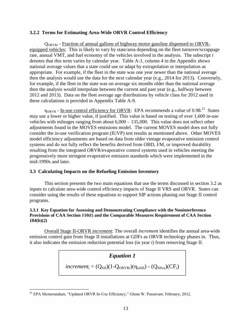
Overall Stage II-ORVR increment: The overall increment identifies the annual area-wide
emission control gain from Stage II installations at GDFs as ORVR technology phases in. Thus,
it also indicates the emission reduction potential loss (in year i) from removing Stage II.
21
EPA Memorandum, “Updated ORVR In-Use Efficiency,” Glenn W. Passavant. February, 2012.
Equation 1
incrementi = (QSII)(1-QORVRi)(ηiuSII) - (QSIIva)(CFi)

14
Under the current regulatory construct for ORVR, there is a small and declining number
of non-ORVR equipped vehicles and thus a small level of future emission reduction achievable
from Stage II. However, due to the vacuum assist compatibility factor, this emission reduction
will eventually go to zero and become negative for states/areas that do not use properly
calibrated ORVR-compatible nozzles because the incompatibility effect will be larger than the
Stage II increment. If the value is greater than zero for the year under consideration there is still
a remaining emission reduction benefit for Stage II for the year relative to ORVR. If it is zero
there is no net difference in the inventory. If it is zero or negative, this would indicate that
removing Stage II would not increase the refueling emissions inventory because the higher
efficiency from ORVR and the incompatibility emissions offset the increment due to non-ORVR
vehicles being refueled at Stage II GDFs. It should be noted that for a state/area with all balance
systems or with a requirement for ORVR compatible nozzles, the CF term is zero.
3.3.2 Key Equation for Assessing and Demonstrating Compliance with CAA Section 193
Overall Stage II - ORVR delta: The overall delta is the comparison between the Stage II
efficiency and the ORVR efficiency with both technologies in place.
This is not the same as the increment calculation in Equation 1 above because it
considers the greater efficiency of ORVR relative to non-ORVR vehicles refueling at Stage II
equipped GDFs.
3.3.3 Developing Area-Specific Values for the Terms Used in Equations 1 and 2
To conduct analyses using Equations 1 and 2, a state would first select a base year or date
for the analysis. The base year or date would correspond to the date the state is considering for
starting to allow decommissioning for affected GDFs. Alternatively, this could be a set of base
years/dates if a state is considering phasing-out Stage II in a specific area over a longer time
period such as two or more years.
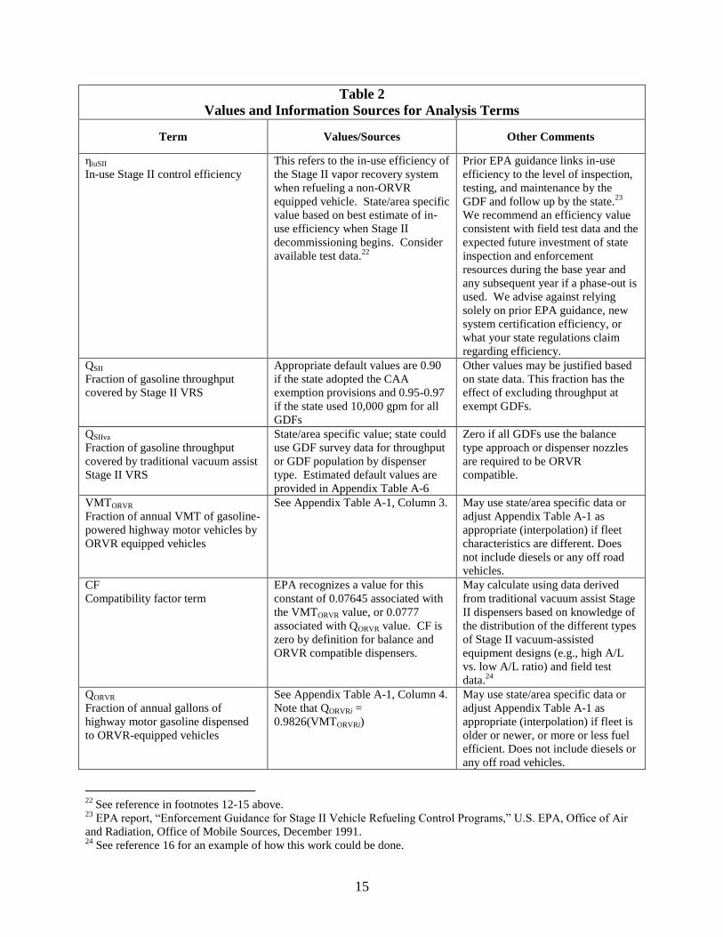
Second, the state would develop the values needed for the equations. The information
and values in Table 2 are provided for consideration.
Equation 2
deltai = (QSII)(ηiuSII) - (QSIIva)(CFi) - (QORVRi)(ηORVR)
15
Table 2
Values and Information Sources for Analysis Terms
Term Values/Sources Other Comments
ηiuSII
In-use Stage II control efficiency
This refers to the in-use efficiency of
the Stage II vapor recovery system
when refueling a non-ORVR
equipped vehicle. State/area specific
value based on best estimate of in-
use efficiency when Stage II
decommissioning begins. Consider
available test data.22
Prior EPA guidance links in-use
efficiency to the level of inspection,
testing, and maintenance by the
GDF and follow up by the state.23
We recommend an efficiency value
consistent with field test data and the
expected future investment of state
inspection and enforcement
resources during the base year and
any subsequent year if a phase-out is
used. We advise against relying
solely on prior EPA guidance, new
system certification efficiency, or
what your state regulations claim
regarding efficiency.
QSII
Fraction of gasoline throughput
covered by Stage II VRS
Appropriate default values are 0.90
if the state adopted the CAA
exemption provisions and 0.95-0.97
if the state used 10,000 gpm for all
GDFs
Other values may be justified based
on state data. This fraction has the
effect of excluding throughput at
exempt GDFs.
QSIIva
Fraction of gasoline throughput
covered by traditional vacuum assist
Stage II VRS
State/area specific value; state could
use GDF survey data for throughput
or GDF population by dispenser
type. Estimated default values are
provided in Appendix Table A-6
Zero if all GDFs use the balance
type approach or dispenser nozzles
are required to be ORVR
compatible.
VMTORVR
Fraction of annual VMT of gasoline-
powered highway motor vehicles by
ORVR equipped vehicles
See Appendix Table A-1, Column 3. May use state/area specific data or
adjust Appendix Table A-1 as
appropriate (interpolation) if fleet
characteristics are different. Does
not include diesels or any off road
vehicles.
CF
Compatibility factor term
EPA recognizes a value for this
constant of 0.07645 associated with
the VMTORVR value, or 0.0777
associated with QORVR value. CF is
zero by definition for balance and
ORVR compatible dispensers.
May calculate using data derived
from traditional vacuum assist Stage
II dispensers based on knowledge of
the distribution of the different types
of Stage II vacuum-assisted
equipment designs (e.g., high A/L
vs. low A/L ratio) and field test
data.24
QORVR
Fraction of annual gallons of
highway motor gasoline dispensed
to ORVR-equipped vehicles
See Appendix Table A-1, Column 4.
Note that QORVRi =
0.9826(VMTORVRi)
May use state/area specific data or
adjust Appendix Table A-1 as
appropriate (interpolation) if fleet is
older or newer, or more or less fuel
efficient. Does not include diesels or
any off road vehicles.
22 See reference in footnotes 12-15 above. 23
EPA report, “Enforcement Guidance for Stage II Vehicle Refueling Control Programs,” U.S. EPA, Office of Air
and Radiation, Office of Mobile Sources, December 1991. 24
See reference 16 for an example of how this work could be done.
16
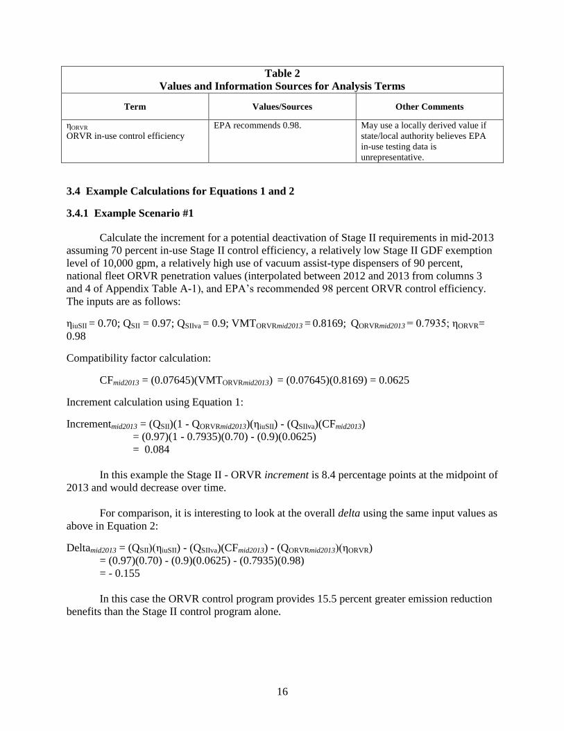
Table 2
Values and Information Sources for Analysis Terms
Term Values/Sources Other Comments
ηORVR
ORVR in-use control efficiency
EPA recommends 0.98. May use a locally derived value if
state/local authority believes EPA
in-use testing data is
unrepresentative.
3.4 Example Calculations for Equations 1 and 2
3.4.1 Example Scenario #1
Calculate the increment for a potential deactivation of Stage II requirements in mid-2013
assuming 70 percent in-use Stage II control efficiency, a relatively low Stage II GDF exemption
level of 10,000 gpm, a relatively high use of vacuum assist-type dispensers of 90 percent,
national fleet ORVR penetration values (interpolated between 2012 and 2013 from columns 3
and 4 of Appendix Table A-1), and EPA’s recommended 98 percent ORVR control efficiency.
The inputs are as follows:
ηiuSII = 0.70; QSII = 0.97; QSIIva = 0.9; VMTORVRmid2013 = 0.8169; QORVRmid2013 = 0.7935; ηORVR=
0.98
Compatibility factor calculation:
CFmid2013 = (0.07645)(VMTORVRmid2013) = (0.07645)(0.8169) = 0.0625
Increment calculation using Equation 1:
Incrementmid2013 = (QSII)(1 - QORVRmid2013)(ηiuSII) - (QSIIva)(CFmid2013)
= (0.97)(1 - 0.7935)(0.70) - (0.9)(0.0625)
= 0.084
In this example the Stage II - ORVR increment is 8.4 percentage points at the midpoint of
2013 and would decrease over time.
For comparison, it is interesting to look at the overall delta using the same input values as
above in Equation 2:
Deltamid2013 = (QSII)(ηiuSII) - (QSIIva)(CFmid2013) - (QORVRmid2013)(ηORVR)
= (0.97)(0.70) - (0.9)(0.0625) - (0.7935)(0.98)
= - 0.155
In this case the ORVR control program provides 15.5 percent greater emission reduction
benefits than the Stage II control program alone.
17
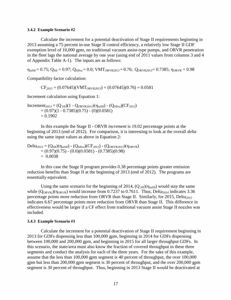
3.4.2 Example Scenario #2
Calculate the increment for a potential deactivation of Stage II requirements beginning in
2013 assuming a 75 percent in-use Stage II control efficiency, a relatively low Stage II GDF
exemption level of 10,000 gpm, no traditional vacuum assist-type pumps, and ORVR penetration
in the fleet lags the national average by one year (using end of 2011 values from columns 3 and 4
of Appendix Table A-1). The inputs are as follows:
ηiuSII = 0.75; QSII = 0.97; QSIIva = 0.0; VMTORVR2013 = 0.76; QORVR2013= 0.7385; ηORVR = 0.98
Compatibility factor calculation:
CF2013 = (0.07645)(VMTORVR2013) = (0.07645)(0.76) = 0.0581
Increment calculation using Equation 1:
Increment2013 = (Q SII)(1 - QORVR2013)(ηiuSII) - (QSIIva)(CF2013)
= (0.97)(1 - 0.7385)(0.75) - (0)(0.0581)
= 0.1902
In this example the Stage II - ORVR increment is 19.02 percentage points at the
beginning of 2013 (end of 2012). For comparison, it is interesting to look at the overall delta
using the same input values as above in Equation 2:
Delta2013 = (QSII)(ηiuSII) - (QSIIva)(CF2013) - (QORVR2013)(ηORVR)
= (0.97)(0.75) - (0.0)(0.0581) - (0.7385)(0.98)
= 0.0038
In this case the Stage II program provides 0.38 percentage points greater emission
reduction benefits than Stage II at the beginning of 2013 (end of 2012). The programs are
essentially equivalent.
Using the same scenario for the beginning of 2014, (Q SII)(ηiuSII) would stay the same
while (QORVRi)(ηORVR) would increase from 0.7237 to 0.7611. Thus, Delta2014 indicates 3.36
percentage points more reduction from ORVR than Stage II. Similarly, for 2015, Delta2015
indicates 6.67 percentage points more reduction from ORVR than Stage II. This difference in
effectiveness would be larger if a CF effect from traditional vacuum assist Stage II nozzles was
included.
3.4.3 Example Scenario #3
Calculate the increment for a potential deactivation of Stage II requirement beginning in
2013 for GDFs dispensing less than 100,000 gpm, beginning in 2014 for GDFs dispensing
between 100,000 and 200,000 gpm, and beginning in 2015 for all larger throughput GDFs. In
this scenario, the state/area must also know the fraction of covered throughput in these three
segments and conduct the analysis for each of the three years. For the sake of this example,
assume that the less than 100,000 gpm segment is 40 percent of throughput, the over 100,000
gpm but less than 200,000 gpm segment is 30 percent of throughput, and the over 200,000 gpm
segment is 30 percent of throughput. Thus, beginning in 2013 Stage II would be deactivated at
18
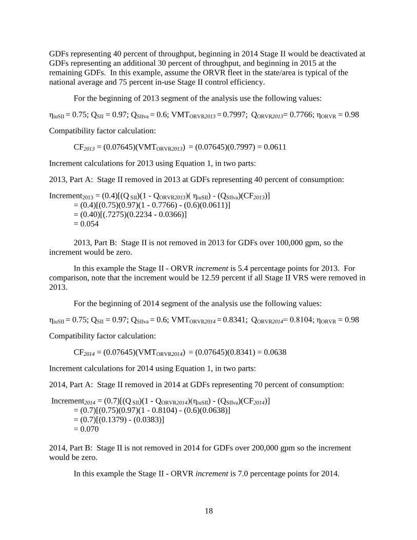
GDFs representing 40 percent of throughput, beginning in 2014 Stage II would be deactivated at
GDFs representing an additional 30 percent of throughput, and beginning in 2015 at the
remaining GDFs. In this example, assume the ORVR fleet in the state/area is typical of the
national average and 75 percent in-use Stage II control efficiency.
For the beginning of 2013 segment of the analysis use the following values:
ηiuSII = 0.75; QSII = 0.97; QSIIva = 0.6; VMTORVR2013 = 0.7997; QORVR2013= 0.7766; ηORVR = 0.98
Compatibility factor calculation:
CF2013 = (0.07645)(VMTORVR2013) = (0.07645)(0.7997) = 0.0611
Increment calculations for 2013 using Equation 1, in two parts:
2013, Part A: Stage II removed in 2013 at GDFs representing 40 percent of consumption:
Increment2013 = (0.4)[(Q SII)(1 - QORVR2013)( ηiuSII) - (QSIIva)(CF2013)]
= (0.4)[(0.75)(0.97)(1 - 0.7766) - (0.6)(0.0611)]
= (0.40)[(.7275)(0.2234 - 0.0366)]
= 0.054
2013, Part B: Stage II is not removed in 2013 for GDFs over 100,000 gpm, so the
increment would be zero.
In this example the Stage II - ORVR increment is 5.4 percentage points for 2013. For
comparison, note that the increment would be 12.59 percent if all Stage II VRS were removed in
2013.
For the beginning of 2014 segment of the analysis use the following values:
ηiuSII = 0.75; QSII = 0.97; QSIIva = 0.6; VMTORVR2014 = 0.8341; QORVR2014= 0.8104; ηORVR = 0.98
Compatibility factor calculation:
CF2014 = (0.07645)(VMTORVR2014) = (0.07645)(0.8341) = 0.0638
Increment calculations for 2014 using Equation 1, in two parts:
2014, Part A: Stage II removed in 2014 at GDFs representing 70 percent of consumption:
Increment2014 = (0.7)[(Q SII)(1 - QORVR2014)(ηiuSII) - (QSIIva)(CF2014)]
= (0.7)[(0.75)(0.97)(1 - 0.8104) - (0.6)(0.0638)]
= (0.7)[(0.1379) - (0.0383)]
= 0.070
2014, Part B: Stage II is not removed in 2014 for GDFs over 200,000 gpm so the increment
would be zero.
In this example the Stage II - ORVR increment is 7.0 percentage points for 2014.

19
For the beginning of 2015 segment of the analysis use the following values:
ηiuSII = 0.75; QSII = 0.97; QSIIva = 0.6; VMTORVR2015 = 0.8633; QORVR2015= 0.8397; ηORVR = 0.98
Compatibility factor calculation:
CF2015 = (0.07645)(VMTORVR2015) = (0.07645)(0.8633) = 0.066
Increment calculations for 2015 using Equation 1:
Increment2015 = (Q SII)(1 - QORVR2015)(ηiuSII) - (QSIIva)(CF2015)
= (0.75)(0.97)(1 - 0.8397) - (0.6)(0.066)
= [(0.1166) - (0.0288)]
= 0.0878
In this example the Stage II - ORVR increment is 8.8 percentage points for 2015 and
would continue to decrease over time. To summarize, the increment values for scenario #3 are:
2013 – 0.054 2014 – 0.070 2015 – 0.088
The cumulative Stage II-ORVR increment for the three years would be 0.21 for the
gradual phase-out scenario which is lower than an increment of 0.30 for the same three year
period if the controls were fully removed in 2013.
3.5 Calculating the Impact on the Area-Wide VOC Inventory
Calculating the impact on the VOC inventory is important in the context of assessing a
SIP action against the provisions of CAA section 110(ℓ), though the methodology in this section
can be applied equally to the outputs of either Equation 1 or Equation 2. The methodology
involves multiplying three different terms, which are area/state specific, as well as appropriate
unit conversion factors, and is shown in Equation 3.
3.5.1 Terms for Calculating Tons VOC
Increment: This is the increment percentage impact on the refueling inventory of
removing Stage II as discussed above, and is the output from Equation 1. The delta percentage
from Equation 2 can also be substituted here.
EF: The uncontrolled displacement refueling emission factor (g/gal). This depends on
the Reid vapor pressure (RVP), dispensed fuel temperature (Td), and the difference between tank
fuel temperature and the dispensed fuel temperature (ΔT). While there are various forms of
equations used to calculate these values we recommend using the equation presented in EPA’s
Equation 3
Tonsi = (Incrementi)(GCi)(EF)

20
ORVR widespread use determination final rule.25
This equation reflects a wider variety of
vehicle models than used in the data set to develop the equation in AP-42. 26
EF (g/gal) = exp[-1.2798 - 0.0049(ΔT) + 0.0203(Td) + 0.1315(RVP)]
where RVP is in psi and temperatures are in °F
There are three terms needed for this calculation. These terms vary by region/state by
month or season. Values used by the EPA for ΔT and Td are contained in the Appendix Tables
A-2 and A-3.27
The RVP value is derived from 40 CFR 80.27 unless there are more specific
state requirements or lower RVP values such as the 7.0 psi RVP gasoline needed to meet the
RFG VOC performance standard. While there is normally some in-use compliance margin for
RVP, to be conservative we recommend that modeling of emissions assume that the in-use RVP
is at the level of the standard. Information on EPA volatility standards and RFG can be found at
the referenced websites.28
States should refer to and rely on any governing federal and state
regulations in lieu of these websites. Default emission factors based on the latest available RVP
information from footnote 28 and temperature information in Tables A-2 and A-3 are provided in
Table A-7 in the Appendix. These were calculated using the equation provided.
GC: The projected gasoline consumption (gal) for the time period(s) and state/area of
interest in gallons. A good publicly available source for information on recent consumption is
the Federal Highway Administration.29
This source provides past gasoline consumption by state
and by month. Information may also be available from other authorities within the state.
Forecast information may be derived from the U.S. Department of Energy’s national annual
forecasts of future gasoline consumption in millions of barrels per day, however, this forecast is
not disaggregated to the state/area level.30
(Note that 1 barrel equals 42 gallons.) A simple
approach for projecting state/area-level consumption would be to apply the national average
growth rate to the latest state-level reported values. States may develop their own approach for
disaggregation or use the state/area gasoline consumption breakouts provided in Table A-4 in the
Appendix. The values in Appendix Table A-4 are EPA estimates based on the ratio of county-
level highway gasoline consumption to national consumption generated from national MOVES
2010b runs based on Department of Energy Annual Energy Outlook 2011 VMT.
25
See EPA Memorandum Onboard Refueling Vapor Recovery Widespread Use Assessment, Glenn W. Passavant,
June 2011. This equation was also used in EPA’s RIA for the original ORVR Final Rule 77 FR 28772, May 16,
2012. 26
Exp is the root of the natural logarithm e, it has a value of 2.71828. In this case it is e raised to the power of the
term in the brackets. 27
See pp. 3-16 to 3-18 of, “Technical Guidance – Stage II Vapor Recovery Systems for Control of Vehicle
Refueling at Gasoline Dispensing Facilities Volume I: Chapters” EPA-450/3-91-022a, November 1991, for basic
information. Additional references are listed in this document. 28
http://www.epa.gov/otaq/fuels/gasolinefuels/volatility/standards.htm 29
Use the latest version available of the DoT FHWA Highway Statistics; see the table entitled “Monthly gasoline
reported by States – MF33GA.” The 2010 version of “Highway Statistics” is found at:
http://www.fhwa.dot.gov/policyinformation/statistics/2010/33ga.cfm 30
Use the motor gasoline projection from the latest version available of the Department of Energy EIA Annual
Energy Outlook (AEO); see the table entitled “Liquid Fuels Supply and Distribution - Reference Case.” The 2011
AEO is found at: http://www.eia.gov/oiaf/aeo/tablebrowser/#release=AEO2011&subject=0-AEO2011&table=11-
AEO2011®ion=0-0&cases=ref2011-d020911a

21
Example 1: Assume we are conducting this calculation for a State in Region 1 of the
EPA fuels temperature matrix for the five-month ozone season May-September, and assume we
are using the Incrementmid2013 value from Example Scenario #1 above, which is 8.4 percentage
points in mid-2013. Since this is an area in Region 1 of the EPA fuels temperature matrix with an
ozone season gasoline RVP of 7.0 psi, the EF calculates to 3.0 g/gal (Td=74°F and ΔT=11.4°F).
Using Table MF-33GA from the 2010 Highway Statistics report, determine Massachusetts’
annual gasoline consumption (i.e., 2,795,148,000 gallons per year). For the five month ozone
season the monthly data in the table indicates that about 43 percent of gasoline is being
consumed during May-September. Growth from 2010-2013 is about 3.44 percent. So, GCmid2013
= 2,795,148,000 * 0.43 * 1.0344 = 1,243,259,400 gal/ozone season.
For the five month ozone season selected here the overall emissions effect of removing
Stage II would be:
Tonsmid2013 = Incrementmid2013 * GCmid2013 * EF * (conversion factors)
= (0.084)(1,243,259,400 gal/season)(3.0 g/gal)[(1 lb/453.59 g)(1 ton/2000 lbs)]
= 341.9 tons/ozone season
In the above equation, in order to obtain an answer in tons per ozone season, we have
introduced conversion factors into the equation where 453.59 grams equal 1 pound, and 2,000
pounds equal 1 ton. These conversion factors are also used in the equation below.
On a daily basis this would be about 2.23 tons per day on average for the 153 days in this
five-month ozone season. There are approximately 3,200 GDFs in Massachusetts with Stage II
VRS. On a daily basis this represents about 1.4 lbs/day per GDF.
States can further disaggregate these calculations to individual ozone nonattainment areas
in the state using the estimates in Appendix Table A-4. The effect would be proportional to
gasoline consumption.
Example 2: Looking at this same Example Scenario #1 above for Deltamid2013, the
emissions impact calculation shows a net gain of tons reduction per ozone season for ORVR
over Stage II alone:
Tonsmid2013 = (0.155)(1,243,259,400 gal/season)(2.97 g/gal)[(1 lb/453.59 g)(1 ton/2000 lbs)]
= 630.9 tons/ozone season
On a daily basis this net difference would be about 4.12 tons per day on average for the
153 days in this five-month ozone season.
3.6 States/Areas with Stage II but not Affected by 182(b)(3) or 184(b)(2)
Portions of six states have implemented Stage II for some areas even though they were
not required to do so under the CAA to meet a requirement under sections 182(b)(3) or
184(b)(2). These include Kentucky, Tennessee, Nevada, California, Oregon, and Washington.
If these states/areas included Stage II-related emission reductions in their SIPs, they will have to
amend their SIPs if Stage II is no longer required, and will have to address the provisions of

22
CAA section 110(ℓ). To facilitate any assessments for SIP revisions (as discussed above), we
have included the relevant input parameters in Table A-8 in the Appendix.
4. Strategies and Considerations for Phasing Out Stage II Controls
Even though EPA has determined that ORVR is in widespread use in the motor vehicle
fleet, and has waived the statutory requirement to implement Stage II programs in ozone
nonattainment areas, states are not obligated to remove the programs. States and local areas may
elect to retain Stage II because it provides VOC and hazardous air pollutant emission reductions
for non-ORVR equipped vehicles. States that wish to phase out Stage II controls do not
necessarily need to wait until the foregone emissions control approaches zero before seeking a
SIP revision. There may come a point where retaining Stage II controls is otherwise unattractive
for cost and cost-effectiveness reasons and, as discussed above, the foregone emission reductions
are small enough that the loss of control would not affect compliance with the NAAQS. This is
especially relevant here since the increment in the first year of Stage II removal will not remain
constant in the future but will continue to decrease going forward in time. This will provide
added assurance that any potential impact on air quality would also diminish. The state would
need to maintain its Stage II program until it is fully phased out and until the state has begun
implementing any needed new measures to ensure there will not be a harmful gap in area-wide
emissions control.
4.1 Gradual Phase-out Strategy
If a state determines that decommissioning all Stage II control in an area all at one time
or by a date certain would result in an unacceptable area-wide emissions increase, then states
might consider a gradual phase-out strategy. A strategy of this nature is illustrated in Example
Scenario #3 above. Using this approach a state might design a phase-out strategy that first
exempts new GDFs from Stage II controls starting in 2013, and provides for subsequent
decommissioning of existing Stage II-equipped GDFs starting with the lowest throughput
stations in 2014 and ending with the highest throughput stations in 2017. An example phase-out
strategy might also use some of the original Stage II program phase-in parameters in CAA
section 182(b)(3) (e.g., new facilities exempted first, then GDFs that dispense less than 100,000
gallons per month, and then all remaining GDFs).
4.2 Cost Considerations
To support their decision making, states may wish to conduct an economic analysis of
their Stage II control program to evaluate the ongoing annualized cost per ton of VOC removed.
The EPA conducted this type of assessment to support the final widespread use determination
rule.31
The EPA estimates that for an average size GDF the annual cost to maintain existing
Stage II systems is about $3,000per year. These total costs would be incurred by GDF operators
each year to cover ever decreasing annual emission reduction benefits as measured by the
increment calculation (Equation 1) described above. The EPA also estimates that the additional
31
See Final Regulatory Support Document - Widespread Use for Onboard Refueling Vapor Recovery and Stage II
Waiver: Decommissioning Stage II Vapor Recovery, Financial Benefits and Costs, March 2012.

23
costs of installing Stage II vapor recovery equipment at new GDFs, which typically include
USTs, associated piping, pumps and ancillary equipment, ranges from $20,000 to $60,000. If
this cost is amortized over a short period of time as ORVR continues to phase-in (e.g., 3 years)
the new control may not be attractive from a cost effectiveness view point.
4.3 Decommissioning Issues
Whatever approach a state decides upon for phasing out Stage II controls, consideration
should be given to proper decommissioning of Stage II-related equipment, including the
underground vapor piping, and to ensuring that consistent procedures are in place to address
liquid and vapor leak issues associated with decommissioning. The EPA recommends that
currently available industry association codes and standards be followed (where applicable) to
ensure that Stage II systems are properly designed, constructed, installed, and, in this case,
dismantled or decommissioned. These codes and standards of practice provide a means for
states to monitor methods of Stage II system decommissioning and we encourage state and local
agencies to reference these codes. The EPA realizes that industry codes and standards may be
updated periodically, and the EPA also recognizes that state and local requirements may
supersede industry codes and standards or be inherently more stringent. The EPA regulations do
not require the use of a particular issue of code. The Petroleum Equipment Institute (PEI) and at
least four states have recommended practices or specific requirements for decommissioning
Stage II systems. The PEI guidance, “Recommended Practices for Installation and Testing of
Vapor Recovery Systems at Vehicle Fueling Sites, PEI/RP300-09,” is especially instructive as it
was developed by industry experts with a focus on regulatory compliance and safety. It contains
the steps involved in dismantling Stage II hardware and applies to both balance and vacuum
assist type systems. Please be aware that there may be other codes or standards not listed here
that may also be appropriate to ensure proper Stage II decommissioning.
4.4 Potential Emission Reduction Programs for GDFs
By viewing the GDF in its entirety as a fuel storage and dispensing system, existing GDF
emissions control systems can be enhanced to achieve a higher level of in-use efficiency, and to
deliver more environmental benefit. Of course, additional system design, maintenance, and
enforcement provisions add cost to the installation and ongoing operation of the systems.
Examples of extra design and monitoring features include: 1) ORVR compatible Stage II
nozzles; 2) systems to help better manage UST pressure and control emissions lost from the UST
through vent lines and fugitive leak sources during normal operations; 3) post processors to
control or eliminate normal UST breathing/emptying loss emissions; 4) standards for specially
designed nozzles that reduce emissions from liquid retention, drips, and spills; and 5) low
permeation fuel hoses.

24
5. Submission, Review and Approval of SIP Revisions
When submitting a SIP revision seeking removal of an existing Stage II vapor recovery
program, the SIP revision package should include the information necessary for the EPA to
determine that the action complies with all relevant CAA provisions, including, as applicable,
sections 110(ℓ), 193, and 184(b)(2). States are encouraged to work closely with EPA Regional
Offices to develop SIP revision packages.
5.1 Elements of SIP Revision Package
The state should coordinate with the appropriate EPA Regional Office on the necessary
format and procedures for submitting a SIP revision. Submittal and cover letters should be
addressed to the EPA Regional Administrator (RA) or the Regional Air Division Director (ADD)
if the RA has delegated that authority to the ADD to accept SIP revisions submittals. The SIP
revision should clearly identify the portion of the state regulation pertaining to the Stage II
regulatory program that the state is requesting to revise. If following this guidance document,
the state could include the results of area-wide emissions and emissions control calculations
based on Equation 1 (increment) and/or Equation 2 (delta). The submittal should also include
analysis, discussion, and any other relevant materials supporting a request for SIP approval with
regards to sections 110(ℓ), 184 (b)(2) and 193, as applicable. If new emissions control
regulations are being adopted to offset emissions controls forgone by the phasing out of a Stage
II program, an analysis of the expected net area-wide emissions change would be appropriate.
5.2 EPA SIP Review Process
The EPA expects that state submission to revise the SIP should show how the revision
satisfies the requirement in section 110(ℓ) not to interfere with attainment or maintenance of the
NAAQS or any other applicable requirement. First, the EPA must determine that the submittal is
complete within 6 months of the submission date. If deemed complete, the EPA must either
approve or disapprove the submittal within one year of the determination of completeness. The
EPA will act on SIP revisions through notice and comment rulemaking.
The EPA is not limited to only considering the calculations presented in this
memorandum when considering a SIP revision seeking to remove Stage II control requirements.
There is no specific value in terms of percentage control or tons of emissions that a state must
meet before EPA can propose to approve a SIP revision. Each SIP revision will be reviewed on
a case-by-case basis against the criteria of CAA section 110(ℓ), and if applicable, sections 193
and/or 184(b)(2), with due consideration to the basis for the values used in supporting
calculations and any related emissions inventory and/or air quality analyses.

25
Appendix
Table A-1 - Projected Penetration of ORVR in the National Gasoline Fueled Vehicle Fleet
by Year
[Based on MOVES 2010(a)]
1 2 3 4
End of Calendar
Year
Vehicle Population
Percentage VMT Percentage
Gasoline Dispensed
Percentage
2006 42.6% 51.2% 49.2%
2007 48.4% 57.3% 55.5%
2008 53.3% 62.3% 60.5%
2009 57.7% 66.8% 64.8%
2010 62.4% 71.6% 69.5%
2011 67.1% 76.0% 73.9%
2012 71.4% 80.0% 77.7%
2013 75.3% 83.4% 81.0%
2014 78.7% 86.3% 84.0%
2015 81.8% 88.8% 86.5%
2016 84.5% 90.9% 88.6%
2017 86.8% 92.5% 90.3%
2018 88.8% 93.9% 91.9%
2019 90.5% 95.0% 93.2%
2020 92.0% 95.9% 94.3%
See EPA Memorandum “Updated data for ORVR Widespread Use Assessment” February 29,
2012, in docket (number EPA-HQ-OAR-2010-1076) addressing details on values in this table
and providing more calendar years.
Note: In this table, the columns have the following meaning.
1. Calendar year that corresponds to the percentages in the row associated with the year.
2. Percentage of the gasoline-powered highway vehicle fleet that have ORVR.
3. Percentage of gasoline-fueled vehicle miles traveled (VMT) by vehicles equipped with
ORVR.
4. Amount of gasoline dispensed into ORVR-equipped vehicles as a percentage of all gasoline
dispensed to highway motor vehicles.

26
Table A-2 - Monthly Average Dispensed Liquid Temperature Dispensed liquid temperature (°F)
Jan Feb Mar Apr May Jun Jul Aug Sep Oct Nov Dec
Weighted Average
Summer
(Apr–Sep)
Winter
(Oct-Mar)
Annual
Average
National
Average 51 54 54 58 69 76 82 81 76 70 62 54 74 58 66
Region 1 43 45 48 53 66 74 78 78 72 66 59 46 70 51 61
Region 2 69 74 73 80 84 87 90 91 78 85 83 73 85 76 81
Region 3 54 57 61 67 76 82 83 84 79 76 67 54 79 62 70
Region 4 50 51 41 47 63 74 88 85 83 75 63 52 74 56 65
Region 5 54 NA NA NA 72 77 83 83 79 74 67 58 79 63 72
Region 6 NA 48 49 53 59 63 NA 73 71 60 49 42 64 50 57
Regional Boundaries
Region 1: ME, VT, NH, MA, CT, RI, NY, NJ, PA, DE, MD,VA,WV,DC, KY, OH, IN, IL, MI, WI
Region 2: NC, SC, GA, FL, AL, MS, AR, LA, TN
Region 3: OK, TX, NM, AZ
Region 4: MN, IA, MO, ND, SD, NE, KS, MT, WY, CO
Region 5: CA, NV, UT
Region 6: WA, OR, ID
Source: McNally Michael and Dickerman J.C., "Summary and Analysis of Data from Gasoline
Temperature Survey," conducted by API, Radian Corporation, May, 1976.
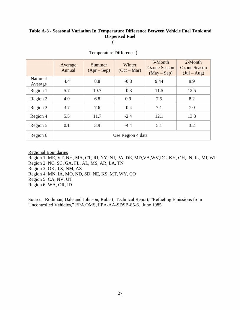
27
Table A-3 - Seasonal Variation In Temperature Difference Between Vehicle Fuel Tank and
Dispensed Fuel
(
Temperature Difference (
Average
Annual
Summer
(Apr – Sep)
Winter
(Oct – Mar)
5-Month
Ozone Season
(May – Sep)
2-Month
Ozone Season
(Jul – Aug)
National
Average 4.4 8.8 -0.8 9.44 9.9
Region 1 5.7 10.7 -0.3 11.5 12.5
Region 2 4.0 6.8 0.9 7.5 8.2
Region 3 3.7 7.6 -0.4 7.1 7.0
Region 4 5.5 11.7 -2.4 12.1 13.3
Region 5 0.1 3.9 -4.4 5.1 3.2
Region 6 Use Region 4 data
Regional Boundaries
Region 1: ME, VT, NH, MA, CT, RI, NY, NJ, PA, DE, MD,VA,WV,DC, KY, OH, IN, IL, MI, WI
Region 2: NC, SC, GA, FL, AL, MS, AR, LA, TN
Region 3: OK, TX, NM, AZ
Region 4: MN, IA, MO, ND, SD, NE, KS, MT, WY, CO
Region 5: CA, NV, UT
Region 6: WA, OR, ID
Source: Rothman, Dale and Johnson, Robert, Technical Report, “Refueling Emissions from
Uncontrolled Vehicles,” EPA.OMS, EPA-AA-SDSB-85-6. June 1985.
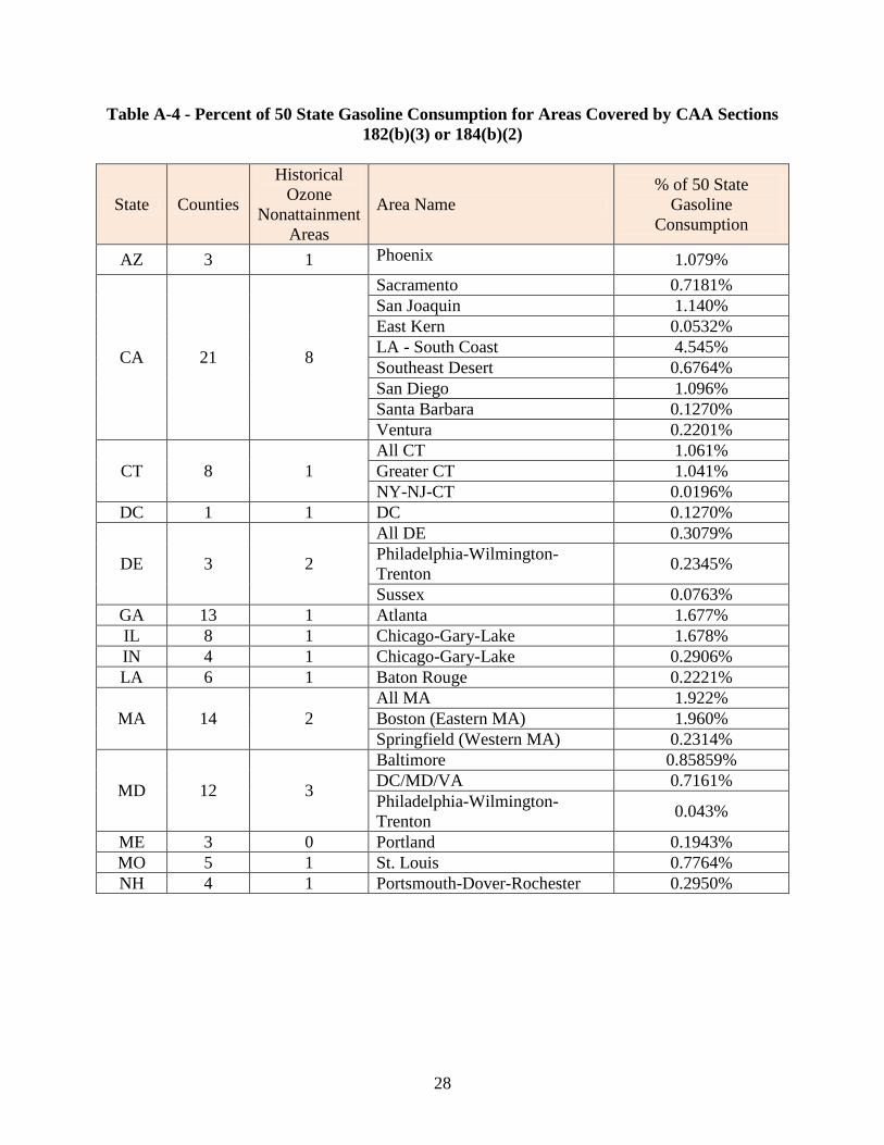
28
Table A-4 - Percent of 50 State Gasoline Consumption for Areas Covered by CAA Sections
182(b)(3) or 184(b)(2)
State Counties
Historical
Ozone
Nonattainment
Areas
Area Name
% of 50 State
Gasoline
Consumption
AZ 3 1 Phoenix 1.079%
CA 21 8
Sacramento 0.7181%
San Joaquin 1.140%
East Kern 0.0532%
LA - South Coast 4.545%
Southeast Desert 0.6764%
San Diego 1.096%
Santa Barbara 0.1270%
Ventura 0.2201%
CT 8 1
All CT 1.061%
Greater CT 1.041%
NY-NJ-CT 0.0196%
DC 1 1 DC 0.1270%
DE 3 2
All DE 0.3079%
Philadelphia-Wilmington-
Trenton 0.2345%
Sussex 0.0763%
GA 13 1 Atlanta 1.677%
IL 8 1 Chicago-Gary-Lake 1.678%
IN 4 1 Chicago-Gary-Lake 0.2906%
LA 6 1 Baton Rouge 0.2221%
MA 14 2
All MA 1.922%
Boston (Eastern MA) 1.960%
Springfield (Western MA) 0.2314%
MD 12 3
Baltimore 0.85859%
DC/MD/VA 0.7161%
Philadelphia-Wilmington-
Trenton 0.043%
ME 3 0 Portland 0.1943%
MO 5 1 St. Louis 0.7764%
NH 4 1 Portsmouth-Dover-Rochester 0.2950%
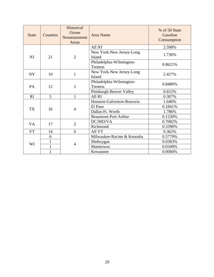
29
State Counties
Historical
Ozone
Nonattainment
Areas
Area Name
% of 50 State
Gasoline
Consumption
NJ 21 2
All NJ 2.598%
New York-New Jersey-Long
Island 1.736%
Philadelphia-Wilmington-
Trenton 0.8621%
NY 10 1 New York-New Jersey-Long
Island 2.427%
PA 12 2
Philadelphia-Wilmington-
Trenton 0.8480%
Pittsburgh-Beaver Valley 0.652%
RI 5 1 All RI 0.307%
TX 16 4
Houston-Galveston-Brazoria 1.646%
El Paso 0.1841%
Dallas-Ft. Worth 1.786%
Beaumont-Port Arthur 0.1230%
VA 17 2 DC/MD/VA 0.7082%
Richmond 0.3390%
VT 14 0 All VT 0.362%
WI
6
4
Milwaukee-Racine & Kenosha 0.5779%
1 Sheboygan 0.0383%
1 Manitowoc 0.0349%
1 Kewaunee 0.0084%

30
Table A-5 - Applicability of Clean Air Act Requirements to Areas Implementing Stage II
Gasoline Vapor Recovery Programs for the Ozone NAAQS
State Nonattainment Areas §110(ℓ)
Only1
§184(b)(2)
(OTR
Comparable
Measures)
§193
(Pre-1990
Savings
Provision)
Attaining
Ozone NAAQS2
1-hour3 1997
8-hour4
2011
DV
2008 8-
hour5
AZ Phoenix X Yes Yes 0.077
No
CA
LA-South Coast X No No 0.107
No
LA-San Bernardino Co (West Mojave Desert)6
X No No 0.097
No
Sacramento Metro X Yes No 0.095
No
San Joaquin Valley6 X No No 0.094
No
Riverside Co (Coachella
Valley)6 X Yes No
0.093 No
Ventura Co X Yes Yes 0.083
No
San Diego X Yes Yes 0.082
No
Santa Barbara-Santa
Maria-Lompoc X Yes Yes
0.076 No
CT NYC-Long Is., NY-NJ-CT X Yes Yes
0.084 No
Greater CT Area X Yes Yes 0.076
No
DE
Philadelphia-Wilmington-
Atlantic City, PA-NJ-MD-DE
X Yes Yes 0.083
No
Sussex County, DE OTR
Area X Yes Yes
0.077 No
GA Atlanta X Yes Yes 0.080
No
IL Chicago-Gary, IL-IN X Yes Yes
0.077 No
St. Louis, MO-IL X Yes Yes 0.077
No
IN Chicago-Gary, IL-IN X Yes Yes 0.077
No
LA Baton Rouge X Yes Yes 0.082
No
ME ME OTR Area X Implementing Stage II in 3
Southern ME Counties. Yes
MD
Baltimore X Yes No 0.092
No
Philadelphia-Wilmington-
Atlantic City, PA-NJ-MD-
DE
X Yes Yes 0.083
No
Washington DC-MD-VA X Yes Yes 0.082
No
MA7
Boston-Lawrence-
Worcester (E. MA) X Yes Yes
0.075 Yes
Springfield (W. MA) X Yes Yes 0.074
Yes
MO St. Louis, MO-IL X Yes Yes 0.079
No
NH
Boston-Lawrence-Worcester (E. MA)
X Yes Yes 0.075
Yes
Portsmouth-Dover-
Rochester X Yes Yes
0.063 Yes
Rest of NH OTR Area X
Implementing Stage II and
RFG to meet comparable measures.
Yes

31
State Nonattainment Areas §110(ℓ)
Only1
§184(b)(2)
(OTR
Comparable
Measures)
§193
(Pre-1990
Savings
Provision)
Attaining
Ozone NAAQS2
1-hour3 1997
8-hour4
2011
DV
2008 8-
hour5
NJ
NYC-Long Is., NY-NJ-CT X X Yes Yes 0.084
No
Philadelphia-Wilmington-
Atlantic City, PA-NJ-MD-DE
X Yes Yes 0.083
No
Rest of NJ OTR Areas X Implementing Stage II in all
counties. Yes
NY NYC-Long Is., NY-NJ-CT X X Yes Yes 0.084
No
PA
Philadelphia-Wilmington-Atlantic City, PA-NJ-MD-
DE
X Yes Yes 0.083
No
Pittsburgh-Beaver Valley,
PA (1-hour Moderate area
under §182(b)(3))
X Yes Yes 0.080
No
RI Providence and all RI
Areas X Yes Yes
0.073 Yes
TX
Houston X No No 0.089
No
Dallas-Ft. Worth X Yes No 0.090
No
Beaumont-Port Arthur X Yes Yes 0.074
Yes
El Paso X Yes Yes 0.071
Yes
VT All of VT (OTR) X Implementing Stage II in all
counties. Yes
VA Washington DC-MD-VA
(Northern VA) X Yes Yes
0.082 No
Richmond, VA X Yes Yes 0.075
Yes
WI Milwaukee-Racine X Yes Yes 0.077
No
1 All states and all areas are required to comply with CAA section 110(ℓ), chart shows states/areas where 110(ℓ) is the only constraint.
2 Based on air quality data from 2009-2011. 3 The 1-hour ozone NAAQS was promulgated in 1979 and was 0.12 ppm. 4 The first 8-hour ozone NAAQS was promulgated in 1997 and is 0.08 ppm and is attained if the area design value is less that or equal to 0.084
ppm. Once an area was designated under the 1997 ozone standard, the 1-hour standard was revoked for that area. As of April 15, 2008, all areas were designated under the 1997 ozone standard. 5 The 2008 8-0hour Ozone NAAQS is 0.075 ppm. 6 History of redistricting and boundary changes between air districts with pre-1990 requirements. District may have Stage II gasoline dispensing rules in some parts of district prior to 1990. 7 The MA Stage II program was adopted prior to 11/15/1990 but was not approved into the SIP until 12/14/1992.

32
Table A-6 - Percent of State/Area GDF Dispensers Using Vacuum Assist Stage II
Technology (June 2012)
State Number
Counties Area name
% GDFs using
Vacuum Assist
ARIZONA 3 Phoenix 85%
CALIFORNIA32
21
Average QSIIva 70%
Sacramento ORVR Compatible
San Joaquin ORVR Compatible
East Kern ORVR Compatible
LA - South Coast ORVR Compatible
Southeast Desert ORVR Compatible
San Diego ORVR Compatible
Santa Barbara ORVR Compatible
Ventura ORVR Compatible
CONNECTICUT 8 All CT 88%
DELAWARE 3 All DE 88%
DC 1 DC 97%
GEORGIA 13 Atlanta 95%
ILLINOIS 8 Chicago metro 92%
INDIANA 4 Chicago-Gary metro 95%
LOUISIANA 6 Baton Rouge 90%
MAINE 3 Portland 95%
MARYLAND 12 Baltimore and Wash DC areas 94%
MASSACHUSETTS 14 All MA 90%
MISSOURI 5 St. Louis 0%
NEW HAMPSHIRE 4 Portsmouth Dover Rochester 93%
NEW JERSEY 21 All NJ 48%
NEW YORK 10 NYC metro 73%
PENNSYLVANIA 12 Philadelphia metro 80%
Pittsburgh -Beaver Valley 96%
RHODE ISLAND 5 All RI 93%
TEXAS33
16
Average QSIIva 90%
Houston-Galveston-Brazoria ORVR Compatible
El Paso ORVR Compatible
Dallas-Fort Worth ORVR Compatible
Beaumont -Port Arthur ORVR Compatible
VIRGINIA 17 Wash DC metro area 93%
Richmond 85%
VERMONT 14 All VT 95%
WISCONSIN 9 All Counties 85%
32
Estimates for California provided by state sources, all vacuum assist must be ORVR compatible. 33
Estimates for Texas provided by state sources, all vacuum assist must be ORVR compatible.
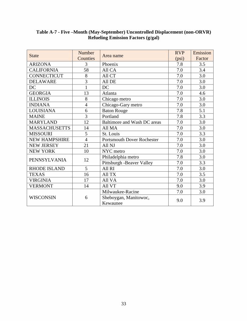
33
Table A-7 - Five –Month (May-September) Uncontrolled Displacement (non-ORVR)
Refueling Emission Factors (g/gal)
State Number
Counties Area name
RVP
(psi)
Emission
Factor
ARIZONA 3 Phoenix 7.8 3.5
CALIFORNIA 58 All CA 7.0 3.4
CONNECTICUT 8 All CT 7.0 3.0
DELAWARE 3 All DE 7.0 3.0
DC 1 DC 7.0 3.0
GEORGIA 13 Atlanta 7.0 4.6
ILLINOIS 8 Chicago metro 7.0 3.0
INDIANA 4 Chicago-Gary metro 7.0 3.0
LOUISIANA 6 Baton Rouge 7.8 5.1
MAINE 3 Portland 7.8 3.3
MARYLAND 12 Baltimore and Wash DC areas 7.0 3.0
MASSACHUSETTS 14 All MA 7.0 3.0
MISSOURI 5 St. Louis 7.0 3.3
NEW HAMPSHIRE 4 Portsmouth Dover Rochester 7.0 3.0
NEW JERSEY 21 All NJ 7.0 3.0
NEW YORK 10 NYC metro 7.0 3.0
PENNSYLVANIA 12 Philadelphia metro 7.8 3.0
Pittsburgh -Beaver Valley 7.0 3.3
RHODE ISLAND 5 All RI 7.0 3.0
TEXAS 16 All TX 7.0 3.5
VIRGINIA 17 All VA 7.0 3.0
VERMONT 14 All VT 9.0 3.9
WISCONSIN 6
Milwaukee-Racine 7.0 3.0
Sheboygan, Manitowoc,
Kewaunee 9.0 3.9

34
Table A-8 - Input Data for States/Areas with Stage II but not Affected by 182(b)(3) or
184(b)(2) (July 2012)
State Number
Counties Area name
Percent of 50
State Gasoline
Consumption
% GDFs
using
Vacuum
Assist34
RVP
(psi)
Five –
Month
(May-
September
Refueling
Emission
Factors
(g/gal)
CALIFORNIA35
37
All AQMDs
& APCDs
not listed in
tables above
2.565% 70% ORVR
Compatible 7.0 3.4
KENTUCKY 3 Jefferson 0.2498% 98% 7.0 3.0
N KY 0.1299% 98% 7.0 3.0
NEVADA 2
Washoe
County 0.1087% 40% 7.8 3.9
Clark
County 0.430% 70% 9.0 4.4
OHIO 16
Cleveland-
Akron 0.8076% 97% 9.0 3.9
Cincinnati 0.4775% 96% 7.8 3.4
Dayton 0.2884% 94% 7.8 3.4
OREGON 3 Portland 0.426% 50% 7.8 3.7
TENNESSEE
1 Davidson 0.2409% 98% 7.8 4.6
4 Nashville
Metro 1.1687% 95% 7.8 4.6
WASHINGTON 5 Seattle 1.088% 80% 9.0 4.3
2 Vancouver 0.1542% 80% 9.0 4.3
34
Estimates for California provided by state sources; all vacuum assist must be ORVR compatible. 35
This data provided by the Petroleum Equipment Institute.

35
Table A-9 – MOVES 2012 Vehicle Class Age Distribution
Calendar Model Gasoline
Year Age Year ID Motorcycle Pass Car LDT1 LDT2 HDGV
2012 30 1982 0.001966 0.000668 0.002037 0.002037 0.005699
2012 29 1983 0.001689 0.000718 0.002178 0.002178 0.005426
2012 28 1984 0.002310 0.001094 0.003234 0.003234 0.006327
2012 27 1985 0.002585 0.001559 0.004318 0.004318 0.008814
2012 26 1986 0.003071 0.002170 0.004989 0.004989 0.011413
2012 25 1987 0.003696 0.002585 0.006043 0.006043 0.009350
2012 24 1988 0.003741 0.003538 0.007146 0.007146 0.011049
2012 23 1989 0.004419 0.004355 0.007774 0.007774 0.011843
2012 22 1990 0.005962 0.005407 0.008745 0.008745 0.010388
2012 21 1991 0.007355 0.006255 0.008972 0.008972 0.009462
2012 20 1992 0.009290 0.008232 0.011363 0.011363 0.011102
2012 19 1993 0.011102 0.011132 0.014774 0.014774 0.014453
2012 18 1994 0.013623 0.015221 0.018422 0.018422 0.020989
2012 17 1995 0.011840 0.018786 0.020574 0.020574 0.023061
2012 16 1996 0.015718 0.023545 0.024745 0.024745 0.025302
2012 15 1997 0.017935 0.028620 0.028422 0.028422 0.027497
2012 14 1998 0.018745 0.034619 0.034691 0.034691 0.032089
2012 13 1999 0.021968 0.044520 0.039503 0.039503 0.045460
2012 12 2000 0.029065 0.054649 0.047137 0.047137 0.048348
2012 11 2001 0.036410 0.056862 0.051960 0.051960 0.052218
2012 10 2002 0.042963 0.057388 0.056257 0.056257 0.047379
2012 9 2003 0.048226 0.056194 0.061399 0.061399 0.052367
2012 8 2004 0.056980 0.057747 0.066770 0.066770 0.058223
2012 7 2005 0.067163 0.060876 0.070393 0.070393 0.064607
2012 6 2006 0.076695 0.063183 0.068310 0.068310 0.063641
2012 5 2007 0.080950 0.062722 0.068566 0.068566 0.063843
2012 4 2008 0.089568 0.056968 0.046968 0.046968 0.048232
2012 3 2009 0.047643 0.051356 0.037902 0.037902 0.040547
2012 2 2010 0.067916 0.061669 0.054558 0.054558 0.052774
2012 1 2011 0.089591 0.070362 0.059917 0.059918 0.057786
2012 0 2012 0.109815 0.076999 0.061931 0.061930 0.060313
Total
1.000000 1.000000 1.000000 1.000000 1.000000
Avg Age
6.9 8.0 8.9 8.9 9.6
LDT1: <6000 lbs GVWR
LDT2 : >6000 but <8500 lbs GVWR
HDGV: > 8500lbs GVWR

36
United States
Environmental Protection
Agency
Office of Air Quality Planning and
Standards
Research Triangle Park, NC
Publication No. EPA-
EPA-457/B-12-001
August 7, 2012
Recommended