Presentation Outline
Introduction
Assumptions
SPSS procedure
Presenting results
Introduction
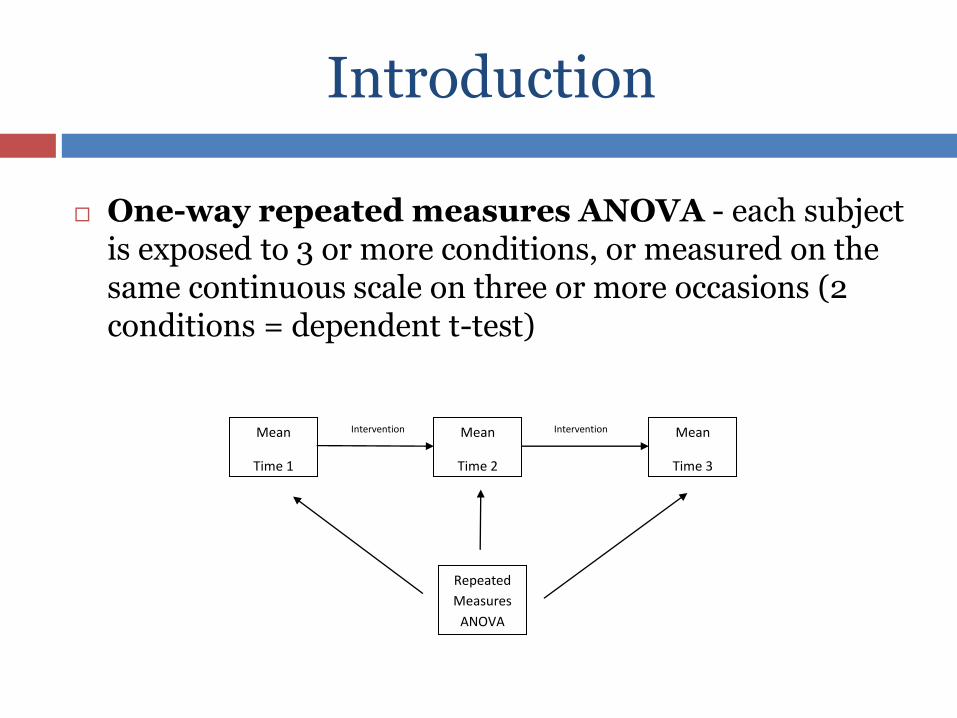
One-way repeated measures ANOVA - each subject is exposed to 3 or more conditions, or measured on the same continuous scale on three or more occasions (2 conditions = dependent t-test)
Mean
Time 1
Mean
Time 2
Mean
Time 3
Repeated
Measures
ANOVA
Intervention Intervention
ONE-WAY Repeated Measures ANOVA
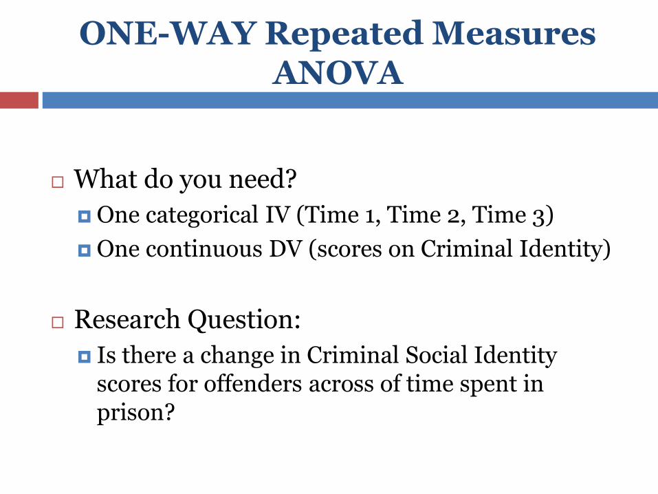
What do you need?
One categorical IV (Time 1, Time 2, Time 3)
One continuous DV (scores on Criminal Identity)
Research Question:
Is there a change in Criminal Social Identity scores for offenders across of time spent in prison?
Assumptions
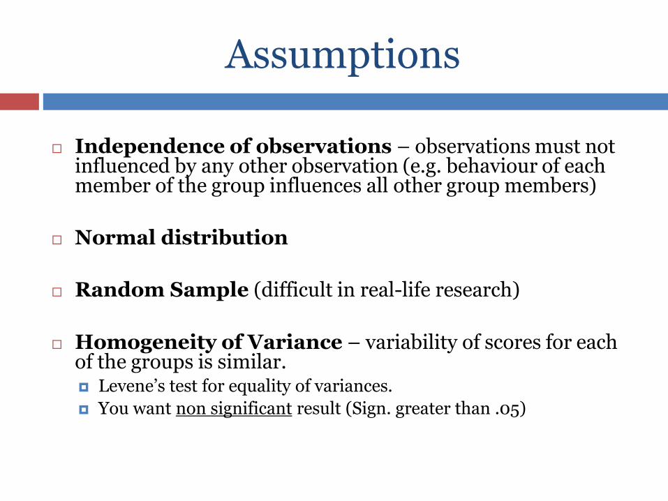
Independence of observations – observations must not influenced by any other observation (e.g. behaviour of each member of the group influences all other group members)
Normal distribution
Random Sample (difficult in real-life research)
Homogeneity of Variance – variability of scores for each of the groups is similar. Levene’s test for equality of variances.
You want non significant result (Sign. greater than .05)
SPSS procedure for One-Way repeated-measures ANOVA
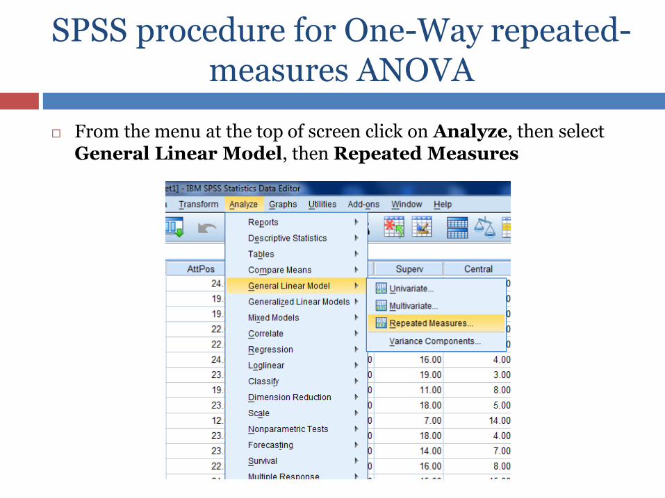
From the menu at the top of screen click on Analyze, then select General Linear Model, then Repeated Measures
SPSS procedure for One-Way repeated-measures ANOVA
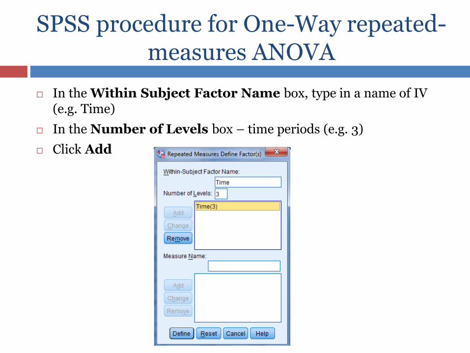
In the Within Subject Factor Name box, type in a name of IV (e.g. Time)
In the Number of Levels box – time periods (e.g. 3)
Click Add
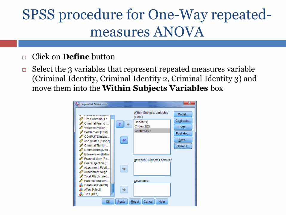
Click on Define button
Select the 3 variables that represent repeated measures variable (Criminal Identity, Criminal Identity 2, Criminal Identity 3) and move them into the Within Subjects Variables box
SPSS procedure for One-Way repeated-measures ANOVA
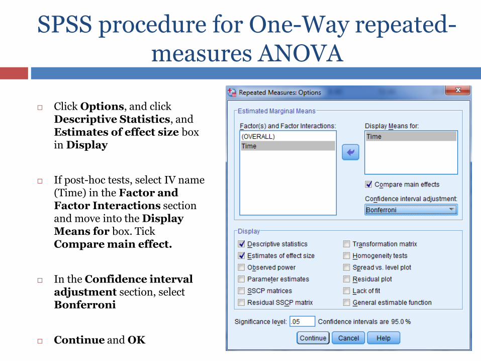
Click Options, and click Descriptive Statistics, and Estimates of effect size box in Display
If post-hoc tests, select IV name (Time) in the Factor and Factor Interactions section and move into the Display Means for box. Tick Compare main effect.
In the Confidence interval adjustment section, select Bonferroni
Continue and OK
SPSS procedure for One-Way repeated-measures ANOVA
Interpretation of SPSS output
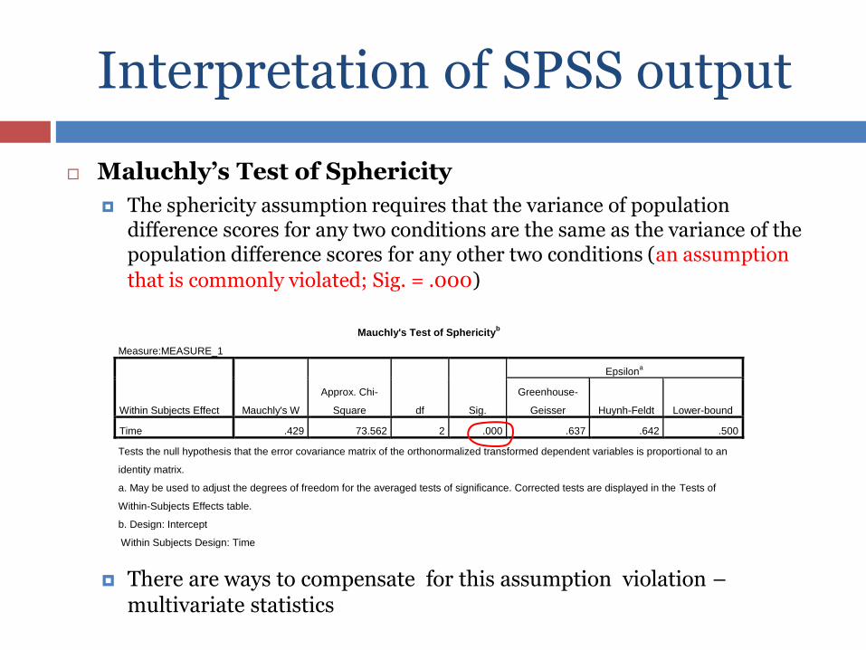
Maluchly’s Test of Sphericity
The sphericity assumption requires that the variance of population difference scores for any two conditions are the same as the variance of the population difference scores for any other two conditions (an assumption
that is commonly violated; Sig. = .000)
There are ways to compensate for this assumption violation – multivariate statistics
Mauchly's Test of Sphericityb
Measure:MEASURE_1
Within Subjects Effect Mauchly's W
Approx. Chi-
Square df Sig.
Epsilona
Greenhouse-
Geisser Huynh-Feldt Lower-bound
Time .429 73.562 2 .000 .637 .642 .500
Tests the null hypothesis that the error covariance matrix of the orthonormalized transformed dependent variables is proportional to an
identity matrix.
a. May be used to adjust the degrees of freedom for the averaged tests of significance. Corrected tests are displayed in the Tests of
Within-Subjects Effects table.
b. Design: Intercept
Within Subjects Design: Time
Interpretation of SPSS output
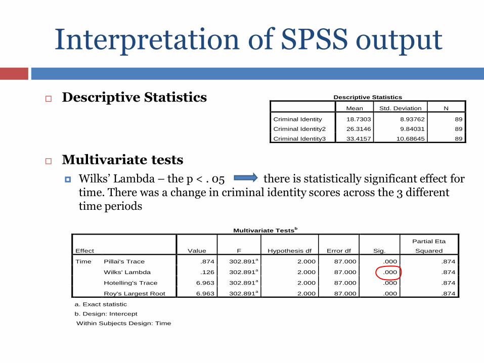
Descriptive Statistics
Mean Std. Deviation N
Criminal Identity 18.7303 8.93762 89
Criminal Identity2 26.3146 9.84031 89
Criminal Identity3 33.4157 10.68645 89
Descriptive Statistics
Multivariate tests
Wilks’ Lambda – the p < . 05 there is statistically significant effect for time. There was a change in criminal identity scores across the 3 different time periods
Multivariate Testsb
Effect Value F Hypothesis df Error df Sig.
Partial Eta
Squared
Time Pillai's Trace .874 302.891a 2.000 87.000 .000 .874
Wilks' Lambda .126 302.891a 2.000 87.000 .000 .874
Hotelling's Trace 6.963 302.891a 2.000 87.000 .000 .874
Roy's Largest Root 6.963 302.891a 2.000 87.000 .000 .874
a. Exact statistic
b. Design: Intercept
Within Subjects Design: Time
Interpretation of SPSS output
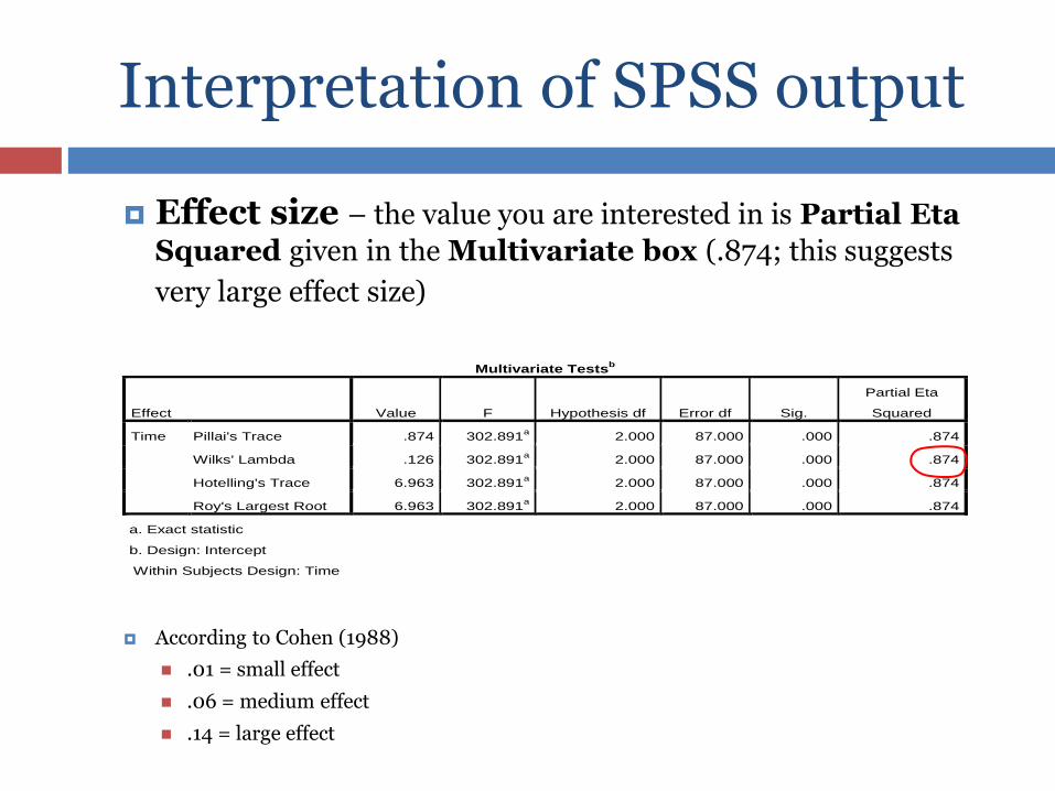
Effect size – the value you are interested in is Partial Eta
Squared given in the Multivariate box (.874; this suggests
very large effect size)
According to Cohen (1988)
.01 = small effect
.06 = medium effect
.14 = large effect
Multivariate Testsb
Effect Value F Hypothesis df Error df Sig.
Partial Eta
Squared
Time Pillai's Trace .874 302.891a 2.000 87.000 .000 .874
Wilks' Lambda .126 302.891a 2.000 87.000 .000 .874
Hotelling's Trace 6.963 302.891a 2.000 87.000 .000 .874
Roy's Largest Root 6.963 302.891a 2.000 87.000 .000 .874
a. Exact statistic
b. Design: Intercept
Within Subjects Design: Time
Interpretation of SPSS output
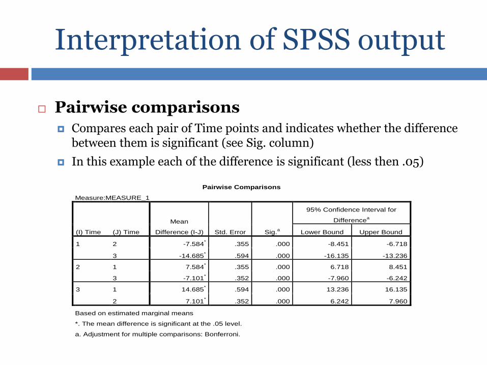
Pairwise comparisons Compares each pair of Time points and indicates whether the difference
between them is significant (see Sig. column)
In this example each of the difference is significant (less then .05)
Pairwise Comparisons
Measure:MEASURE_1
(I) Time (J) Time
Mean
Difference (I-J) Std. Error Sig.a
95% Confidence Interval for
Differencea
Lower Bound Upper Bound
1 2 -7.584* .355 .000 -8.451 -6.718
3 -14.685* .594 .000 -16.135 -13.236
2 1 7.584* .355 .000 6.718 8.451
3 -7.101* .352 .000 -7.960 -6.242
3 1 14.685* .594 .000 13.236 16.135
2 7.101* .352 .000 6.242 7.960
Based on estimated marginal means
*. The mean difference is significant at the .05 level.
a. Adjustment for multiple comparisons: Bonferroni.
Presenting results
A one-way repeated measures analysis of variance was conducted in order to compare scores of criminal social identity among prisoners with a statistic test at time 1 (prior to intervention), time 2 (after intervention), and time 3 (three months follow-up). The means and standard deviations are presented in Table 1. There was a significant effect for time, Wilks’ Lambda = .13, F (2, 87) = 302.89, p < .0005, multivariate partial squared = .874. The results suggest that criminal social identity reported by prisoners significantly increased over time.

Presenting results
Table
Plot
Table 1. Descriptive Statistics for Criminal Social Identity with Statistics Test for Time 1,
Time 2, and Time 3
Time period M SD N
Time 1
Time 2
Time 3
18.73
26.31
33.42
8.94
9.84
10.67
89
89
89
Recommended