Online Knowledge-Based Support

Vector Machines

Gautam Kunapuli∗, Kristin P. Bennett†, Amina Shabbeer†,Richard Maclin‡ and Jude Shavlik∗

∗University of Wisconsin-Madison, †Rensselaer Polytechnic Insitute, and‡University of Minnesota, Duluth

Abstract. Prior knowledge, in the form of simple advice rules, cangreatly speed up convergence in learning algorithms. Online learningmethods predict the label of the current point and then receive the cor-rect label (and learn from that information). The goal of this work is toupdate the hypothesis taking into account not just the label feedback,but also the prior knowledge, in the form of soft polyhedral advice, soas to make increasingly accurate predictions on subsequent examples.Advice helps speed up and bias learning so that generalization can beobtained with less data. Our passive-aggressive approach updates thehypothesis using a hybrid loss that takes into account the margins ofboth the hypothesis and the advice on the current point. Encouragingcomputational results and loss bounds are provided.

1 Introduction

We propose a novel online learning method that incorporates advice into passive-aggressive algorithms, which we call the Adviceptron. Learning with advice andother forms of inductive transfer have been shown to improve machine learningby introducing bias and reducing the number of samples required. Prior work hasshown that advice is an important and easy way to introduce domain knowledgeinto learning; this includes work on knowledge-based neural networks [15] andprior knowledge via kernels [12]. More specifically, for SVMs [16], knowledgecan be incorporated in three ways [13]: by modifying the data, the kernel or theunderlying optimization problem. While we focus on the last approach, we directreaders to a recent survey [9] on prior knowledge in SVMs.

Despite advances to date, research has not addressed how to incorporateadvice into incremental SVM algorithms from either a theoretical or computa-tional perspective. In this work, we leverage the strengths of Knowledge-BasedSupport Vector Machines (KBSVMs) [6] to effectively incorporate advice intothe passive-aggressive framework introduced by Crammer et al., [4]. Our workexplores the various difficulties and challenges in incorporating prior knowledgeinto online approaches and serves as a template to extending these techniquesto other online algorithms. Consequently, we present an appealing frameworkfor generalizing KBSVM-type formulations to online algorithms with simple,closed-form weight-update formulas and known convergence properties.

2

We focus on the binary classification problem and demonstrate the in-corporation of advice that leads to a new algorithm called the passive-aggressiveAdviceptron. In the Adviceptron, as in KBSVMs, advice is specified for convex,polyhedral regions in the input space of data. As shown in Fung et al., [6], advicetakes the form of (a set of) simple, possibly conjunctive, implicative rules. Ad-vice can be specified about every potential data point in the input space whichsatisfies certain advice constraints, such as the rule

(feature7 ≥ 5) ∧ (feature12 ≥ 4) ⇒ (class = +1),

which states that the class should be +1 when feature7 is at least 5 andfeature12 is at least 4. Advice can be specified for individual features as aboveand for linear combinations of features, while the conjunction of multiple rulesallows more complex advice sets. However, just as label information of data canbe noisy, the advice specification can be noisy as well. The purpose of advice istwofold: first, it should help the learner reach a good solution with fewer trainingdata points, and second, advice should help the learner reach a potentially bettersolution (in terms of generalization to future examples) than might have beenpossible learning from data alone.

We wish to study the generalization of KBSVMs to the online case withinthe well-known framework of passive-aggressive algorithms (PAAs, [4]). Given aloss function, the algorithm is passive whenever the loss is zero, i.e., the datapoint at the current round t is correctly classified. If misclassified, the algorithmupdates the weight vector (wt) aggressively, such that the loss is minimized overthe new weights (wt+1). The update rule that achieves this is derived as theoptimal solution to a constrained optimization problem comprising two terms: aloss function, and a proximal term that requires wt+1 to be as close as possible towt. There are several advantages of PAAs: first, they readily apply to standardSVM loss functions used for batch learning. Second, it is possible to deriveclosed-form solutions and consequently, simple update rules. Third, it is possibleto formally derive relative loss bounds where the loss suffered by the algorithmis compared to the loss suffered by some arbitrary, fixed hypothesis.

We evaluate the performance of the Adviceptron on two real-world tasks:diabetes diagnosis, and Mycobacterium tuberculosis complex (MTBC) isolateclassification into major genetic lineages based on DNA fingerprints. The lattertask is an essential part of tuberculosis (TB) tracking, control, and research byhealth care organizations worldwide [7]. MTBC is the causative agent of tuber-culosis, which remains one of the leading causes of disease and morbidity world-wide. Strains of MTBC have been shown to vary in their infectivity, transmissioncharacteristics, immunogenicity, virulence, and host associations depending ontheir phylogeographic lineage [7]. MTBC biomarkers or DNA fingerprints areroutinely collected as part of molecular epidemiological surveillance of TB. Clas-sification of strains of MTBC into genetic lineages can help implement suitablecontrol measures. Currently, the United States Centers for Disease Control andPrevention (CDC) routinely collect DNA fingerprints for all culture positive TBpatients in the United States. Dr. Lauren Cowan at the CDC has developed

3

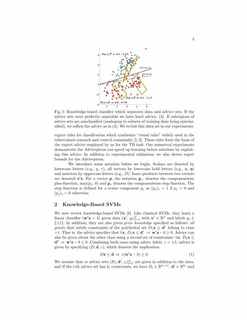
Fig. 1: Knowledge-based classifier which separates data and advice sets. If theadvice sets were perfectly separable we have hard advice, (3). If subregions ofadvice sets are misclassified (analogous to subsets of training data being misclas-sified), we soften the advice as in (4). We revisit this data set in our experiments.

expert rules for classification which synthesize “visual rules” widely used in thetuberculosis research and control community [1, 3]. These rules form the basis ofthe expert advice employed by us for the TB task. Our numerical experimentsdemonstrate the Adviceptron can speed up learning better solutions by exploit-ing this advice. In addition to experimental validation, we also derive regretbounds for the Adviceptron.

We introduce some notation before we begin. Scalars are denoted bylowercase letters (e.g., y, τ), all vectors by lowercase bold letters (e.g., x, η)and matrices by uppercase letters (e.g., D). Inner products between two vectorsare denoted x′z. For a vector p, the notation p+ denotes the componentwiseplus-function, max(pj , 0) and p⋆ denotes the componentwise step function. Thestep function is defined for a scalar component pj as (pj)⋆ = 1 if pj > 0 and(pj)⋆ = 0 otherwise.

2 Knowledge-Based SVMs

We now review knowledge-based SVMs [6]. Like classical SVMs, they learn alinear classifier (w′x = b) given data (xt, yt)

Tt=1 with xt ∈ R

n and labels yt ∈{±1}. In addition, they are also given prior knowledge specified as follows: allpoints that satisfy constraints of the polyhedral set D1x ≤ d1 belong to class+1. That is, the advice specifies that ∀x, D1x ≤ d1 ⇒ w′x− b ≥ 0. Advice canalso be given about the other class using a second set of constraints: ∀x, D2x ≤d2 ⇒ w′x− b ≤ 0. Combining both cases using advice labels, z = ±1, advice isgiven by specifying (D,d, z), which denotes the implication

Dx ≤ d ⇒ z(w′x− b) ≥ 0. (1)

We assume that m advice sets (Di,di, zi)

mi=1 are given in addition to the data,

and if the i-th advice set has ki constraints, we have Di ∈ Rki×n, di ∈ R

ki and

4

zi = {±1}. Figure 1 provides an example of a simple two-dimensional learningproblem with both data and polyhedral advice.

Note that due to the implicative nature of the advice, it says nothingabout points that do not satisfy Dx ≤ d. Also note that the notion of margincan easily be introduced by requiring that Dx ≤ d ⇒ z(w′x − b) ≥ γ, i.e.,that the advice sets (and all the points contained in them) be separated by amargin of γ analogous to the notion of margin for individual data points. Advicein implication form cannot be incorporated into an SVM directly; this is done byexploiting theorems of the alternative [11]. Observing that p ⇒ q is equivalentto ¬p ∨ q, we require that the latter be true; this is same as requiring that thenegation (p ∧ ¬q) be false or that the system of equations

{Dx − d τ ≤ 0, zw′x − zb τ < 0, −τ < 0} has no solution (x, τ). (2)

The variable τ is introduced to bring the system to nonhomogeneous form. Usingthe nonhomogeneous Farkas theorem of the alternative [11] it can be shown that(2) is equivalent to

{D′u + zw = 0, −d′u− zb ≥ 0, u ≥ 0} has a solution u. (3)

The set of (hard) constraints above incorporates the advice specified by a singlerule/advice set. As there are m advice sets, each of the m rules is added as theequivalent set of constraints of the form (3). When these are incorporated into astandard SVM, the formulation becomes a hard-KBSVM; the formulation is hardbecause the advice is assumed to be linearly separable, that is, always feasible.Just as in the case of data, linear separability is a very limiting assumption andcan be relaxed by introducing slack variables (ηi and ζi) to soften the constraints(3). If P and L are some convex regularization and loss functions respectively,the full soft-advice KBSVM is

minimize(ξ,ui,ηi,ζi)≥0,w,b

P(w) + λLdata(ξ) + µm∑

i=1

Ladvice(ηi, ζi)

subject to Y (Xw − be) + ξ ≥ e,D′

iui + ziw + ηi = 0,

−di′ui − zib + ζi ≥ 1, i = 1, . . . , m,

(4)

where X is the T × n set of data points to be classified with labels y ∈ {±1}T ,Y = diag(y) and e is a vector of ones of the appropriate dimension. The variablesξ are the standard slack variables that allow for soft-margin classification of thedata. There are two regularization parameters λ, µ ≥ 0, which tradeoff the dataand advice errors with the regularization.

While converting the advice from implication to constraints, we intro-duced new variables for each advice set: the advice vectors ui ≥ 0. The advicevectors perform the same role as the dual multipliers α in the classical SVM.Recall that points with non-zero α’s are the support vectors which additivelycontribute to w. Here, for each advice set, the constraints of the set which havenon-zero uis are called support constraints.

5

3 Passive-Aggressive Algorithms with Advice

We are interested in an online version of (4) where the algorithm is given Tlabeled points (xt, yt)

Tt=1 sequentially and required to update the model hy-

pothesis, wt, as well as the advice vectors, ui,t, at every iteration. The batchformulation (4) can be extended to an online passive-aggressive formulation byintroducing proximal terms for the advice variables, ui:

arg minξ,ui,ηi,ζi,w

1

2‖w − wt‖2 +

1

2

m∑

i=1

‖ui − ui,t‖2 +λ

2ξ2 +

µ

2

m∑

i=1

(‖ηi‖2 + ζ2

i

)

subject to ytw′xt − 1 + ξ ≥ 0,

D′iu

i + ziw + ηi = 0

−di′ui − 1 + ζi ≥ 0

ui ≥ 0

i = 1, . . . , m.

(5)

Notice that while L1 regularization and losses were used in the batch version [6],we use the corresponding L2 counterparts in (5). This allows us to derive passive-aggressive closed-form solutions. We address this illustrative and effective specialcase, and leave the general case of dynamic online learning of advice and weightvectors for general losses as future work.

Directly deriving the closed-form solutions for (5) is impossible owing tothe fact that satisfying the many inequality constraints at optimality is a com-binatorial problem which can only be solved iteratively. To circumvent this, weadopt a two-step strategy when the algorithm receives a new data point (xt, yt):first, fix the advice vectors ui,t in (5) and use these to update the weight vectorwt+1, and second, fix the newly updated weight vector in (5) to update the ad-vice vectors and obtain ui,t+1, i = 1, . . . , m. While many decompositions of thisproblem are possible, the one considered above is arguably the most intuitiveand leads to an interpretable solution and also has good regret minimizing prop-erties. In the following subsections, we derive each step of this approach and inthe section following, analyze the regret behavior of this algorithm.

3.1 Updating w Using Fixed Advice Vectors ui,t

At step t (= 1, . . . , T ), the algorithm receives a new data point (xt, yt). Thehypothesis from the previous step is wt, with corresponding advice vectors ui,t,i = 1, . . . , m, one for each of the m advice sets. In order to update wt basedon the advice, we can simplify the formulation (5) by fixing the advice variablesui = ui,t. This gives a fixed-advice online passive-aggressive step, where thevariables ζi drop out of the formulation (5), as do the constraints that involvethose variables. We can now solve the following problem (the correspondingLagrange multipliers for each constraint are indicated in parentheses):

wt+1 = minimizew,ξ,ηi

1

2‖w − wt‖2

2 +λ

2ξ2 +

µ

2

m∑

i=1

‖ηi‖22

subject to ytw′xt − 1 + ξ ≥ 0, (α)

D′iu

i + ziw + ηi = 0, i = 1, . . . , m. (βi)

(6)

6

In (6), D′iu

i is the classification hypothesis according to the i-th knowledgeset. Multiplying D′

iui by the label zi, the labeled i-th hypothesis is denoted

ri = −ziD′iu

i. We refer to the ris as the advice-estimates of the hypothesisbecause they represent each advice set as a point in hypothesis space. We willsee later that the next step when we update the advice using the fixed hypothesiscan be viewed as representing the hypothesis-estimate of the advice as a pointin that advice set. The effect of the advice on w is clearly through the equalityconstraints of (6) which force w at each round to be as close to each of theadvice-estimates as possible by aggressively minimizing the error, ηi. Moreover,Theorem 1 proves that the optimal solution to (6) can be computed in closed-form and that this solution requires only the centroid of the advice estimates,r = (1/m)

∑m

i=1 ri. For fixed advice, the centroid or average advice vector r,provides a compact and sufficient summary of the advice.

Update Rule 1 (Computing wt+1 from ui,t) For λ, µ > 0, and given ad-vice vectors ui,t ≥ 0, let rt = 1/m

∑m

i=1 ri,t = −1/m∑m

i=1 ziD′iu

i,t, withν = 1/(1 + mµ). Then, the optimal solution of (6) which also gives the closed-form update rule is given by

wt+1 = w

t + αtytxt +

m∑

i=1

ziβi,t = ν (wt + αtytx

t) + (1 − ν) rt,

αt =

(1 − ν ytw

t′xt − (1 − ν) ytrt′xt

)

+

1

λ+ ν‖xt‖2

,ziβ

i,t

µ= r

i,t − wt + αt⋆ λytxt + mµ rt

1

ν+ αt⋆ λ‖xt‖2

.

(7)

The numerator of αt is the combined loss function,

ℓt = max(

1 − ν ytwt′xt − (1 − ν) ytr

t′xt, 0)

, (8)

which gives us the condition upon which the update is implemented. This isexactly the hinge loss function where the margin is computed by a convex com-bination of the current hypothesis wt and the current advice-estimate of thehypothesis rt. Note that for any choice of µ > 0, the value of ν ∈ (0, 1] withν → 0 as µ → ∞. Thus, ℓt is simply the hinge loss function applied to a con-vex combination of the margin of the hypothesis, wt from the current iterationand the margin of the average advice-estimate, rt. Furthermore, if there is noadvice, m = 0 and ν = 1, and the updates above become exactly identical toonline passive-aggressive algorithms for support vector classification [4]. Also, itis possible to eliminate the variables βi from the expressions (7) to give a verysimple update rule that depends only on αt and rt:

wt+1 = ν(wt + αtytxt) + (1 − ν)rt. (9)

This update rule is a convex combination of the current iterate updated by thedata, xt and the advice, rt.

7

3.2 Updating ui,t Using the Fixed Hypothesis wt+1

When w is fixed to wt+1, the master problem breaks up into m smaller sub-problems, the solution of each one yielding updates to each of the ui for the i-thadvice set. The i-th subproblem (with the corresponding Lagrange multipliers)is shown below:

ui,t+1 = arg minui,η,ζ

1

2‖ui − ui,t‖2 +

µ

2

(‖ηi‖2

2 + ζ2i

)

subject to D′iu

i + ziwt + ηi = 0, (βi)

−di′ui − 1 + ζi ≥ 0, (γi)

ui ≥ 0. (τ i)

(10)

The first-order gradient conditions can be obtained from the Lagrangian:

ui = ui,t + Diβi − diγi + τ i, ηi =

βi

µ, ζi =

γi

µ. (11)

The complicating constraints in the above formulation are the cone constraintsui ≥ 0. If these constraints are dropped, it is possible to derive a closed-formintermediate solution, ui ∈ R

ki . Then, observing that τ i ≥ 0, we can computethe final update by projecting the intermediate solution onto ui ≥ 0.

ui,t+1 =(ui,t + Diβ

i − diγi

)+

. (12)

When the constraints ui ≥ 0 are dropped from (10), the resulting problem can besolved (analogous to the derivation of the update step for wt+1) to give a closed-form solution which depends on the dual variables: ui,t+1 = ui,t + Diβ

i − diζi.This solution is then projected into the positive orthant by applying the plusfunction: ui,t+1 = ui,t+1

+ . This leads to the advice updates, which need to appliedto each advice vector ui,t, i = 1, . . . , m individually.

Update Rule 2 (Computing ui,t+1 from wt+1) For µ > 0, and given thecurrent hypothesis wt+1, for each advice set, i = 1, . . . , m, the update rule isgiven by

ui,t+1 =

(u

i,t + Diβi − d

iγi

)

+

,

[βi

γi

]= H−1

i gi,

Hi,t =

−(D′

iDi + 1

µIn) D′

idi

di′Di −(di′di + 1

µ)

, gi,t =

D′iu

i,t + ziwt

−di′ui,t − 1

, (13)

with the untruncated solution being the optimal solution to (10) without the coneconstraints ui ≥ 0.

Recall that, when updating the hypothesis wt using new data points xt and thefixed advice (i.e., ui,t is fixed), each advice set contributes an estimate of the

hypothesis (rti= −ziD

′iu

i,t) to the update. We termed the latter the advice-estimate of the hypothesis. Here, given that when there is an update, β 6= 0,

8

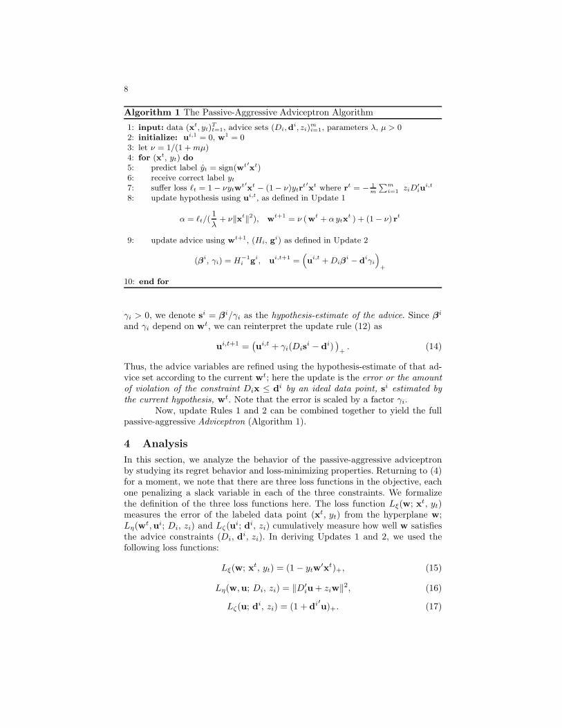
Algorithm 1 The Passive-Aggressive Adviceptron Algorithm

1: input: data (xt, yt)Tt=1, advice sets (Di,d

i, zi)mi=1, parameters λ, µ > 0

2: initialize: ui,1 = 0, w1 = 03: let ν = 1/(1 + mµ)4: for (xt, yt) do

5: predict label yt = sign(wt′xt)6: receive correct label yt

7: suffer loss ℓt = 1 − νytwt′xt − (1 − ν)ytr

t′xt where rt = − 1

m

∑m

i=1ziD

′iu

i,t

8: update hypothesis using ui,t, as defined in Update 1

α = ℓt/(1

λ+ ν‖xt‖2), w

t+1 = ν (wt + α ytxt ) + (1 − ν) rt

9: update advice using wt+1, (Hi, gi) as defined in Update 2

(βi, γi) = H−1

i gi, u

i,t+1 =(u

i,t + Diβi − d

iγi

)

+

10: end for

γi > 0, we denote si = βi/γi as the hypothesis-estimate of the advice. Since βi

and γi depend on wt, we can reinterpret the update rule (12) as

ui,t+1 =(ui,t + γi(Dis

i − di))+

. (14)

Thus, the advice variables are refined using the hypothesis-estimate of that ad-vice set according to the current wt; here the update is the error or the amountof violation of the constraint Dix ≤ di by an ideal data point, si estimated bythe current hypothesis, wt. Note that the error is scaled by a factor γi.

Now, update Rules 1 and 2 can be combined together to yield the fullpassive-aggressive Adviceptron (Algorithm 1).

4 Analysis

In this section, we analyze the behavior of the passive-aggressive adviceptronby studying its regret behavior and loss-minimizing properties. Returning to (4)for a moment, we note that there are three loss functions in the objective, eachone penalizing a slack variable in each of the three constraints. We formalizethe definition of the three loss functions here. The loss function Lξ(w; xt, yt)measures the error of the labeled data point (xt, yt) from the hyperplane w;Lη(wt,ui; Di, zi) and Lζ(u

i; di, zi) cumulatively measure how well w satisfiesthe advice constraints (Di, di, zi). In deriving Updates 1 and 2, we used thefollowing loss functions:

Lξ(w; xt, yt) = (1 − ytw′xt)+, (15)

Lη(w,u; Di, zi) = ‖D′iu + ziw‖2, (16)

Lζ(u; di, zi) = (1 + di′u)+. (17)

9

Also, in the context of (4), Ldata = 12L2

ξ and Ladvice = 12 (Lη + L2

ζ). Note that inthe definitions of the loss functions, the arguments after the semi-colon are thedata and advice, which are fixed.

Lemma 1. At round t, if we define the updated advice vector before projectionfor the i-th advice set as ui, the following hold for all w ∈ R

n:

1. ui = ui,t − µ∇uiLadvice(ui,t),

2. ‖∇uiLadvice(ui,t)‖2 ≤

(‖Di‖

2Lη(ui,t,w) + ‖di‖2L2ζ(u

i,t))

.

The first inequality above can be derived from the definition of the loss functionsand the first-order conditions (11). The second inequality follows from the firstcondition using convexity: ‖∇uiLadvice(u

i,t)‖2 = ‖Diηi−diγi‖

2 = ‖Di(D′iu

i,t +

ziwt+1) + di(di′ui,t + 1)‖2 ≤ ‖Di(D

′iu

i,t + ziwt+1)‖2 + ‖di(di′ui,t + 1)‖2. The

inequality follows by applying ‖Ax‖ ≤ ‖A‖‖x‖. We now state additional lemmasthat can be used to derive the final regret bound. The proofs are in the appendix.

Lemma 2. Consider the rules given in Update 1, with w1 = 0 and λ, µ > 0.For all w∗ ∈ R

n we have

‖w∗ − wt+1‖2 − ‖w∗ − wt‖2 ≤

νλLξ(w∗)2 −

νλ

1 + νλX2Lξ(w

t)2 + (1 − ν)‖w∗ − rt‖2.

where wt = νwt + (1− ν)rt, the combined hypothesis that determines if there isan update, ν = 1/(1 + mµ), and we assume that ‖xt‖2 ≤ X2, ∀t = 1, . . . , T .

Lemma 3. Consider the rules given in Update 2, for the i-th advice set withui,1 = 0, and µ > 0. For all u∗ ∈ R

ki

+ , we have

‖u∗ − ui,t+1‖2 − ‖u∗ − ui,t‖2 ≤ µLη(u∗,wt) + µLζ(u∗)2

−µ((1 − µ∆2)Lη(ui,t,wt) + (1 − µδ2)Lζ(u

i,t)2).

where we assume that ‖Di‖2 ≤ ∆2 and ‖di‖2 ≤ δ2.

Lemma 4. At round t, given the current hypothesis and advice vectors wt andui,t, for any w∗ ∈ R

n and ui,∗ ∈ Rki

+ , i = 1, . . . , m, we have

‖w∗ − rt‖2 ≤1

m

m∑

i=1

Lη(w∗,ui,t) =1

m

m∑

i=1

‖w∗ − ri,t‖2

The overall loss suffered over one round t = 1, . . . , T is defined as follows:

R(w,u; c1, c2, c3) =

(c1Lξ(w)2 +

m∑

i=1

(c2Lη(w,u) + c3Lζ(u)2)

).

This is identical to the loss functions defined in the batch version of KBSVMs(4) and its online counterpart (10). The Adviceptron was derived such that it

10

minimizes the latter. The lemmas are used to prove the following regret boundfor the Adviceptron1.

Theorem 1. Let S = {(xt, yt)}Tt=1 be a sequence of examples with (xt, yt) ∈

Rn × {±1}, and ‖xt‖2 ≤ X ∀t. Let A = {(Di, di, zi)}

mi=1 be m advice sets

with ‖Di‖2 ≤ ∆ and ‖di‖2 ≤ δ. Then the following holds for all w∗ ∈ Rn and

ui ∈ Rki

+ :

1

T

T∑

t=1

R

(wt,ut;

λ

1 + νλX2, µ(1 − µ∆2), µ(1 − µδ2)

)

≤1

T

T∑

t=1

R(w∗,u∗; λ, 0, µ) + R(w∗,ut; 0, µ, 0) + R(wt+1,u∗; 0, µ, 0)

+1

νT‖w∗‖2 +

1

T

M∑

i=1

‖ui,∗‖2.

(18)

If the last two R terms in the right hand side are bounded by 2R(w∗,u∗; 0, µ, 0),then the regret behavior becomes similar to truncated-gradient algorithms [8].

5 Experiments

We performed experiments on three data sets: one artificial (see Figure 1) andtwo real world. Our real world data sets are Pima Indians Diabetes data setfrom the UCI repository [2] and M. tuberculosis spoligotype data set (both aredescribed below). We also created a synthetic data set where one class of the datacorresponded to a mixture of two small σ Gaussians and the other (overlapping)class was represented by a flatter (large σ) Gaussian. For this set, the learner isprovided with three hand-made advice sets (see Figure 1).

5.1 Diabetes Data Set

The diabetes data set consists of 768 points with 8 attributes. For domain ad-vice, we constructed two rules based on statements from the NIH web site on risksfor Type-2 Diabetes2. A person who is obese, characterized by high body massindex (BMI ≥ 30) and high bloodglucose level (≥ 126) is at strong risk for dia-betes, while a person who is at normal weight (BMI ≤ 25) and low bloodglucose

level (≤ 100) is unlikely to have diabetes. As BMI and bloodglucose are featuresof the data set, we can give advice by combining these conditions into conjunc-tive rules, one for each class. For instance, the rule predicting that diabetes isfalse is (BMI ≤ 25) ∧ (bloodglucose≤ 100) ⇒ ¬diabetes.

5.2 Tuberculosis Data Set

These data sets consist of two types of DNA fingerprints of M. tuberculosis com-plex (MTBC): the spacer oglionucleotide types (spoligotypes) and Mycobacterial

1 The complete derivation can be found at http://ftp.cs.wisc.edu/machine-

learning/shavlik-group/kunapuli.ecml10.proof.pdf2 http://diabetes.niddk.nih.gov/DM/pubs/riskfortype2

11

#pieces of #pieces ofClass #isolates Positive Advice Negative Advice

East-Asian 4924 1 1East-African-Indian 1469 2 4Euro-American 25161 1 2Indo-Oceanic 5309 5 5M. africanum 154 1 3M. bovis 693 1 3

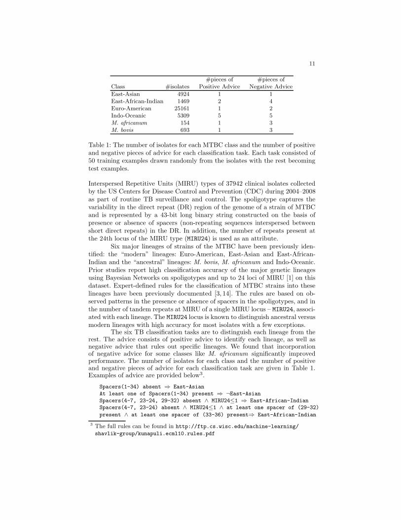
Table 1: The number of isolates for each MTBC class and the number of positiveand negative pieces of advice for each classification task. Each task consisted of50 training examples drawn randomly from the isolates with the rest becomingtest examples.

Interspersed Repetitive Units (MIRU) types of 37942 clinical isolates collectedby the US Centers for Disease Control and Prevention (CDC) during 2004–2008as part of routine TB surveillance and control. The spoligotype captures thevariability in the direct repeat (DR) region of the genome of a strain of MTBCand is represented by a 43-bit long binary string constructed on the basis ofpresence or absence of spacers (non-repeating sequences interspersed betweenshort direct repeats) in the DR. In addition, the number of repeats present atthe 24th locus of the MIRU type (MIRU24) is used as an attribute.

Six major lineages of strains of the MTBC have been previously iden-tified: the “modern” lineages: Euro-American, East-Asian and East-African-Indian and the “ancestral” lineages: M. bovis, M. africanum and Indo-Oceanic.Prior studies report high classification accuracy of the major genetic lineagesusing Bayesian Networks on spoligotypes and up to 24 loci of MIRU [1] on thisdataset. Expert-defined rules for the classification of MTBC strains into theselineages have been previously documented [3, 14]. The rules are based on ob-served patterns in the presence or absence of spacers in the spoligotypes, and inthe number of tandem repeats at MIRU of a single MIRU locus – MIRU24, associ-ated with each lineage. The MIRU24 locus is known to distinguish ancestral versusmodern lineages with high accuracy for most isolates with a few exceptions.

The six TB classification tasks are to distinguish each lineage from therest. The advice consists of positive advice to identify each lineage, as well asnegative advice that rules out specific lineages. We found that incorporationof negative advice for some classes like M. africanum significantly improvedperformance. The number of isolates for each class and the number of positiveand negative pieces of advice for each classification task are given in Table 1.Examples of advice are provided below3.

Spacers(1-34) absent ⇒ East-Asian

At least one of Spacers(1-34) present ⇒ ¬East-AsianSpacers(4-7, 23-24, 29-32) absent ∧ MIRU24≤1 ⇒ East-African-Indian

Spacers(4-7, 23-24) absent ∧ MIRU24≤1 ∧ at least one spacer of (29-32)

present ∧ at least one spacer of (33-36) present⇒ East-African-Indian

3 The full rules can be found in http://ftp.cs.wisc.edu/machine-learning/

shavlik-group/kunapuli.ecml10.rules.pdf

12

Spacers(3, 9, 16, 39-43) absent ∧ spacer 38 present ⇒ M. bovis

Spacers(8, 9, 39) absent ∧ MIRU24>1 ⇒ M. africanum

Spacers(3, 9, 16, 39-43) absent ∧ spacer 38 present ⇒ ¬ M. africanum

For each lineage, both negative and positive advice can be naturally expressed.For example, the positive advice for M. africanum closely corresponds to a knownrule: if spacers(8, 9, 13) are absent ∧ MIRU24 ≤1⇒ M. africanum. How-ever, this rule is overly broad and is further refined by exploiting the fact that M.africanum is an ancestral strain. Thus, the following rules out all modern strains:if MIRU24 ≤ 1 ⇒ ¬ M. africanum. The negative advice captures the fact thatspoligotypes do not regain spacers once lost. For example, if at least one of

Spacers(8, 9, 39) is present ⇒ ¬ M. africanum. The final negative rulerules out M. bovis, a close ancestral strain easily confused with M. africanum.

5.3 Methodology

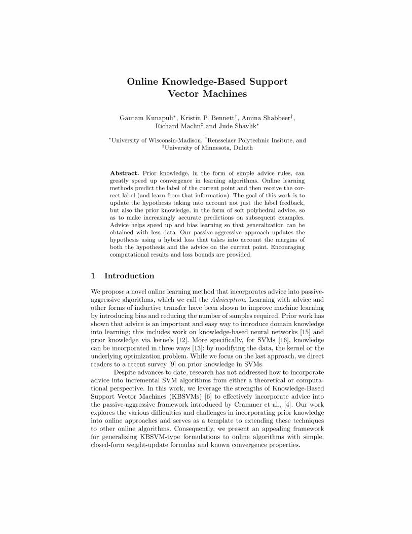
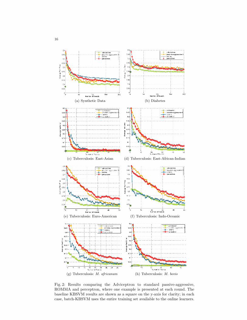
The results for each data set are averaged over multiple randomized iterations(20 iterations for synthetic and diabetes, and 200 for the tuberculosis tasks).For each iteration of the synthetic and diabetes data sets, we selected 200points at random as the training set and used the rest as the test set. For eachiteration of the tuberculosis data sets, we selected 50 examples at randomfrom the data set to use as a training set and tested on the rest. Each time, thetraining data was presented in a random order, one example at a time, to thelearner to generate the learning curves shown in Figures 2(a)–2(h). We comparethe results to well-studied incremental algorithms: standard passive-aggressivealgorithms [4], margin-perceptron [5] and ROMMA [10]. We also compare it tothe standard batch KBSVM [6], where the learner was given all of the examplesused in training the online learners (e.g., for the synthetic data we had 200 datapoints to create the learning curve, so the KBSVM used those 200 points).

5.4 Analysis of Results

For both artificial and real world data sets, the advice leads to significantly fasterconvergence of accuracy over the no-advice approaches. This reflects the intuitiveidea that a learner, when given prior knowledge that is useful, will be able tomore quickly find a good solution. In each case, note also, that the learner is ableto use the learning process to improve on the starting accuracy (which wouldbe produced by advice only). Thus, the Adviceptron is able to learn effectivelyfrom both data and advice.

A second point to note is that, in some cases, prior knowledge allowsthe learner to converge on a level of accuracy that is not achieved by the othermethods, which do not benefit from advice. While the results demonstrate thatadvice can make a significant difference when learning with small data sets, inmany cases, large amounts of data may be needed by the advice-free algorithmsto eventually achieve performance similar to the Adviceptron. This shows thatadvice can provide large improvements over just learning with data.

13

Finally, it can be seen that, in most cases, the generalization performanceof the Adviceptron converges rapidly to that of the batch-KBSVM. However,the batch-KBSVMs take, on average, 15–20 seconds to compute an optimalsolution as they have to solve a quadratic program. In contrast, owing to thesimple, closed-form update rules, the Adviceptron is able to obtain identical test-set performance in under 5 seconds on average. Further scalability experimentsrepresent one of the more immediate directions of future work. One minor pointto note is regarding the results on East-Asian and M. bovis (Figures 2(e) and2(h)): the advice (provided by a tuberculosis domain expert) was so effective thatthese problems were almost immediately learned (with few to no examples).

6 Conclusions and Related Work

We have presented a new online learning method, the Adviceptron, that is a novelapproach that makes use of prior knowledge in the form of polyhedral advice.This approach is an online extension to KBSVMs [6] and differs from previouspolyhedral advice-taking approaches and the neural-network-based KBANN [15]in two significant ways: it is an online method with closed-form solutions and itprovides a theoretical mistake bound.

The advice-taking approach was incorporated into the passive-aggressiveframework because of its many appealing properties including efficient updaterules and simplicity. Advice updates in the adviceptron are computed usinga projected-gradient approach similar to the truncated-gradient approaches byLangford et al., [8]. However, the advice updates are truncated far more aggres-sively. The regret bound shows that as long as the projection being consideredis non-expansive, it is still possible to minimize regret.

We have presented a bound on the effectiveness of this method and aproof of that bound. In addition, we performed several experiments on artificialand real world data sets that demonstrate that a learner with reasonable advicecan significantly outperform a learner without advice. We believe our approachcan serve as a template for other methods to incorporate advice into onlinelearning methods.

One drawback of our approach is the restriction to certain types of lossfunctions. More direct projected-gradient approach or other related online con-vex programming [17] approaches can be used to develop algorithms with similarproperties. This also allows for the derivation of general algorithms for differentloss functions. KBSVMs can also be extended to kernels as shown in [6], and isyet another direction of future work.

Acknowledgements

The authors would like to thank Dr. Lauren Cowan of the CDC for providing the

TB dataset and the expert-defined rules for lineage classification. The authors grate-

fully acknowledge support of the Defense Advanced Research Projects Agency under

DARPA grant FA8650-06-C-7606 and the National Institute of Health under NIH grant

14

1-R01-LM009731-01. Views and conclusions contained in this document are those of

the authors and do not necessarily represent the official opinion or policies, either

expressed or implied of the US government or of DARPA.

References

1. M. Aminian, A. Shabbeer, and K. P. Bennett. A conformal Bayesian network forclassification of Mycobacterium tuberculosis complex lineages. BMC Bioinformat-

ics, 11(Suppl 3):S4, 2010.2. A. Asuncion and D.J. Newman. UCI machine learning repository, 2007.3. K. Brudey, J.R. Driscoll, L. Rigouts, W.M. Prodinger, A. Gori, S.A. Al-Hajoj,

C. Allix, L. Aristimuno, J. Arora, V. Baumanis, et al. Mycobacterium tuberculosis

complex genetic diversity: Mining the fourth international spoligotyping database(spoldb 4) for classification, population genetics and epidemiology. BMC Microbi-

ology, 6(1):23, 2006.4. K. Crammer, O. Dekel, J. Keshet, S. Shalev-Shwartz, and Y. Singer. Online

passive-aggressive algorithms. J. of Mach. Learn. Res., 7:551–585, 2006.5. Y. Freund and R. E. Schapire. Large margin classification using the perceptron

algorithm. Mach. Learn., 37(3):277–296, 1999.6. G. Fung, O. L. Mangasarian, and J. W. Shavlik. Knowledge-based support vector

classifiers. In S. Becker, S. Thrun, and K. Obermayer, editors, NIPS, volume 15,pages 521–528, 2003.

7. S. Gagneux and P. M. Small. Global phylogeography of Mycobacterium tubercu-losis and implications for tuberculosis product development. The Lancet Infectious

Diseases, 7(5):328–337, 2007.8. J. Langford, L. Li, and T. Zhang. Sparse online learning via truncated gradient.

J. Mach. Learn. Res., 10:777–801, 2009.9. F. Lauer and G. Bloch. Incorporating prior knowledge in support vector machines

for classification: A review. Neurocomp., 71(7-9):1578–1594, 2008.10. Y. Li and P. M. Long. The relaxed online maximum margin algorithm. Mach.

Learn., 46(1/3):361–387, 2002.11. O. L. Mangasarian. Nonlinear Programming. McGraw-Hill, 1969.12. B. Scholkopf, P. Simard, A. Smola, and V. Vapnik. Prior knowledge in support

vector kernels. In NIPS, volume 10, pages 640–646, 1998.13. B. Scholkopf and A. Smola. Learning with Kernels: Support Vector Machines,

Regularization Optimization and Beyond. MIT Press, Cambridge, MA, USA, 2001.14. A. Shabbeer, L. Cowan, J. R. Driscoll, C. Ozcaglar, S. L Vandenberg, B. Yener,

and K. P Bennett. TB-Lineage: An online tool for classification and analysis ofstrains of Mycobacterium tuberculosis Complex. Unpublished manuscript, 2010.

15. G. G. Towell and J. W. Shavlik. Knowledge-based artificial neural networks. Ar-

tificial Intelligence, 70(1-2):119–165, 1994.16. V. Vapnik. The Nature of Statistical Learning Theory. Springer-Verlag, 2000.17. M. Zinkevich. Online convex programming and generalized infinitesimal gradient

ascent. In Proc. 20th Int. Conf. on Mach. Learn., 2003.

Appendix

Proof of Lemma 2

The progress at trial t is ∆t = 1

2‖w∗ − wt+1‖2 − 1

2‖w∗ − wt‖2 =

1

2‖wt+1 − w

t‖2 +

(wt − w∗)′(wt+1 − w

t). Substituting wt+1 − wt = ν αtytxt + (1 − ν)(rt − wt), from

15

the update rules, we have

∆t ≤ 1

2ν2α2

t‖xt‖2 + ναt

(ν ytw

t′x

t + (1 − ν) ytrt′x

t − ytw∗′x

t)

+1

2(1 − ν) ‖rt − w

∗‖2.

The loss suffered by the adviceptron is defined in (8). We focus only on the casewhen the loss is > 0. Define wt = νwt + (1 − ν)rt. Then, we have 1 − Lξ(w

t) =ν ytw

t′xt + (1 − ν) ytrt′xt. Furthermore, by definition, Lξ(w

∗) ≥ 1 − ytw∗′xt. Using

these two results,

∆t ≤ 1

2ν2α2

t‖xt‖2 + ν αt(Lξ(w∗) − Lξ(w

t)) +1

2(1 − ν) ‖rt − w

∗‖2. (19)

Adding 1

2ν ( αt√

λ−√

λℓ∗t )2 to the left-hand side of the and simplifying, using Update 1:

∆t ≤ 1

2

ν Lξ(wt)2(

1

λ+ ν ‖xt‖2

) − 1

2ν λLξ(w

∗)2

+1

2(1 − ν) ‖rt − w

∗‖2.

Rearranging the terms above and using ‖xt‖2 ≤ X2 gives the bound. �

Proof of Lemma 3

Let ui,t = ui,t + Diβi − diγi be the update before the projection onto u ≥ 0. Then,

ui,t+1 = ui,t+ . We also write Ladvice(u

i,t) compactly as L(ui,t). Then,

1

2‖u∗ − u

i,t+1‖2 ≤ 1

2‖u∗ − u

i,t‖2

=1

2‖u∗ − u

i,t‖2 +1

2‖ui,t − u

i,t‖2 + (u∗ − ui,t)′(ui,t − u

i,t)

=1

2‖u∗ − u

i,t‖2 +µ2

2‖∇

uiL(ui,t)‖2 + µ(u∗ − u

i,t)′∇u

iL(ui,t)

The first inequality is due to the non-expansiveness of projection and the next stepsfollow from Lemma 1.1. Let ∆t = 1

2‖u∗ − ui,t+1‖2 − 1

2‖u∗ − ui,t‖2. Using Lemma 1.2,

we have

∆t ≤ µ2

2

(‖Di‖2Lη(ui,t, wt) + ‖di‖2Lζ(u

i,t)2)

+µ(u∗ − ui,t)′(

1

2∇

uiLη(ui,t, wt) + Lζ(u

i,t)∇u

iLζ(ui,t)

)

≤ µ2

2

(‖Di‖2Lη(ui,t, wt) + ‖di‖2Lζ(u

i,t)2)

+µ

2

(Lη(u∗, wt) − Lη(ui,t,wt)

)+

µ

2

(Lζ(u

∗)2 − Lζ(ui,t)2

)

where the last step follows from the convexity of the loss function Lη and the fact that

Lζ(ui,t)(u∗ − ui,t)′∇

uiLζ(u

i,t)

≤ Lζ(ui,t)(Lζ(u

∗) − Lζ(ui,t))

(convexity of Lζ)

≤ Lζ(ui,t)(Lζ(u

∗) − Lζ(ui,t))

+1

2

(Lζ(u

∗) − Lζ(ui,t))2

.

Rearranging the terms and bounding ‖Di‖2 and ‖di‖2 proves the lemma. �

16

(a) Synthetic Data (b) Diabetes

(c) Tuberculosis: East-Asian (d) Tuberculosis: East-African-Indian

(e) Tuberculosis: Euro-American (f) Tuberculosis: Indo-Oceanic

(g) Tuberculosis: M. africanum (h) Tuberculosis: M. bovis

Fig. 2: Results comparing the Adviceptron to standard passive-aggressive,ROMMA and perceptron, where one example is presented at each round. Thebaseline KBSVM results are shown as a square on the y-axis for clarity; in eachcase, batch-KBSVM uses the entire training set available to the online learners.