NAVAL
POSTGRADUATE
SCHOOL
MONTEREY, CALIFORNIA
THESIS
Approved for public release; distribution is unlimited
SIMULATING THE SPREAD OF AN OUTBREAK OF FOOT AND MOUTH DISEASE IN CALIFORNIA
by
Brian S. Axelsen
June 2012
Thesis Advisor: Nedialko B. Dimitrov Second Readers: David Alderson Pam Hullinger Mark Stevenson

THIS PAGE INTENTIONALLY LEFT BLANK

i
REPORT DOCUMENTATION PAGE Form Approved OMB No. 0704-0188Public reporting burden for this collection of information is estimated to average 1 hour per response, including the time for reviewing instruction, searching existing data sources, gathering and maintaining the data needed, and completing and reviewing the collection of information. Send comments regarding this burden estimate or any other aspect of this collection of information, including suggestions for reducing this burden, to Washington headquarters Services, Directorate for Information Operations and Reports, 1215 Jefferson Davis Highway, Suite 1204, Arlington, VA 22202-4302, and to the Office of Management and Budget, Paperwork Reduction Project (0704-0188) Washington DC 20503.
1. AGENCY USE ONLY (Leave blank)
2. REPORT DATE June 2012
3. REPORT TYPE AND DATES COVERED Master’s Thesis
4. TITLE AND SUBTITLE Simulating the Spread of an Outbreak of Foot and Mouth Disease in California
5. FUNDING NUMBERS
6. AUTHOR(S) Brian S. Axelsen
7. PERFORMING ORGANIZATION NAME(S) AND ADDRESS(ES) Naval Postgraduate School Monterey, CA 93943-5000
8. PERFORMING ORGANIZATION REPORT NUMBER
9. SPONSORING /MONITORING AGENCY NAME(S) AND ADDRESS(ES) N/A
10. SPONSORING/MONITORING AGENCY REPORT NUMBER
11. SUPPLEMENTARY NOTES The views expressed in this thesis are those of the author and do not reflect the official policy or position of the Department of Defense or the U.S. Government. IRB Protocol number ______N/A______.
12a. DISTRIBUTION / AVAILABILITY STATEMENT Approved for public release; distribution is unlimited
12b. DISTRIBUTION CODE A
13. ABSTRACT (maximum 200 words) Foot and mouth disease (FMD) is a highly contagious viral disease affecting cloven-hoofed domestic and some wild animals. A hypothetical outbreak of FMD begun in California was recently estimated to have a national impact of up to $55 billion, mostly due to international trade restrictions (Carpenter, O’Brien, Hagerman, & McCarl, 2011). Therefore, preparedness for an outbreak is a high priority within the livestock industry, and state and federal government.
We use simulation and a designed experiment to identify robust governmental and industrial surveillance response strategies to control the spread of FMD. A strategy is considered robust if it is effective across a number of outbreak scenarios and a variety of disease spread characteristics.
The main contributions of this thesis are: (1) the development of FMD outbreak scenarios across California that can be used in conjunction with a state-of-the-art, animal disease simulation model, and (2) the development and analysis of an efficient experimental design that allows for the identification of key parameters affecting the spread and containment of an FMD outbreak.
The analysis of over 400,000 simulations in the experimental design indicates two key areas for the control ofFMD:
(1) surveillance activities at dairy and dairy-like premises are a dominant factor in early identification of the disease and increased surveillance leads to lower impacts of an outbreak; and (2) fast initial response and capacity of depopulation resources are also key factors in controlling an FMD outbreak, even when no preemptive depopulation strategies are considered.
14. SUBJECT TERMS Foot and mouth disease, disease modeling, simulation analysis, nearly orthogonal and balanced design, design of experiment, California, InterSpread Plus
15. NUMBER OF PAGES
159
16. PRICE CODE
17. SECURITY CLASSIFICATION OF REPORT
Unclassified
18. SECURITY CLASSIFICATION OF THIS PAGE
Unclassified
19. SECURITY CLASSIFICATION OF ABSTRACT
Unclassified
20. LIMITATION OF ABSTRACT
UU
NSN 7540-01-280-5500 Standard Form 298 (Rev. 2-89) Prescribed by ANSI Std. 239-18

ii
THIS PAGE INTENTIONALLY LEFT BLANK

iii
Approved for public release; distribution is unlimited
SIMULATING THE SPREAD OF AN OUTBREAK OF FOOT AND MOUTH DISEASE IN CALIFORNIA
Brian S. Axelsen Lieutenant Colonel, United States Army Reserve
B.B.A., Texas Christian University, 1994
Submitted in partial fulfillment of the requirements for the degree of
MASTER OF SCIENCE IN OPERATIONS RESEARCH
from the
NAVAL POSTGRADUATE SCHOOL June 2012
Author: Brian S. Axelsen
Approved by: Nedialko B. Dimitrov
Thesis Advisor
David Alderson Second Reader
Pam Hullinger Second Reader Mark Stevenson Second Reader
Robert F. Dell Chair, Department of Operations Research

iv
THIS PAGE INTENTIONALLY LEFT BLANK
v
ABSTRACT
Foot and mouth disease (FMD) is a highly contagious viral disease affecting cloven-
hoofed domestic and some wild animals. An A hypothetical outbreak of FMD begun in
California was recently estimated to have a national impact of up to $55 billion, mostly
due to international trade restrictions (Carpenter, O’Brien, Hagerman, & McCarl,
Carpenter et al., 2011 ). Therefore, preparedness for an outbreak is a high priority within
the livestock industry, and state and federal government.
We use simulation and a designed experiment to identify robust governmental and
industrial surveillance response strategies to control the spread of FMD. A strategy is
considered robust if it is effective across a number of outbreak scenarios and a variety of
disease spread characteristics.
The main contributions of this thesis are: (1) the development of FMD outbreak
scenarios across California that can be used in conjunction with a state-of-the-art, animal
disease simulation model, and (2) the development and analysis of an efficient
experimental design that allows for the identification of key parameters affecting the
spread and containment of an FMD outbreak.
The analysis of over 400,000 simulations in the experimental design indicates two
key areas for the control of FMD: (1) surveillance activities at dairy and dairy-like
premises are a dominant factor in early identification of the disease and increased
surveillance leads to lower impacts of an outbreak, and (2) fast initial responsiveness
response and capacity of depopulation resources are also a key factors in controlling an
FMD outbreak, even when no pre-emptive depopulation strategies are considered.

vi
THIS PAGE INTENTIONALLY LEFT BLANK
vii
TABLE OF CONTENTS
I. INTRODUCTION........................................................................................................1 A. PURPOSE .........................................................................................................1 B. BACKGROUND ..............................................................................................2 C. CURRENT PREVENTION AND RESPONSE STRATEGIES
AGAINST FMD ...............................................................................................3 1. Prevention .............................................................................................3 2. Detection ...............................................................................................4 3. Selection of a Control Strategy ...........................................................5 4. Management of the Control Strategy .................................................6
D. LITERATURE REVIEW ...............................................................................9 E. RESEARCH QUESTIONS ...........................................................................10
II. METHODOLOGY AND DATA DEVELOPMENT ..............................................13 A. SIMULATION MODELLING OF FOOT AND MOUTH DISEASE
(FMD) ..............................................................................................................13 1. Why Model? .......................................................................................13 2. Choosing a Simulation Software Package or Simulation Model ...14 3. Characteristics of the Chosen Model ...............................................15
B. DATA DESCRIPTION .................................................................................18 1. Description of the Dataset .................................................................18 2. Our Procedure to Interpret and Modify the Dataset for Use in
ISP 20 a. The Farm File .........................................................................21 b. The Contact Location File ......................................................26 c. The Epidemic History File ......................................................27 d. The Zone File ..........................................................................27
C. SIMULATION SOFTWARE PARAMETER AND INITIAL INFECTION SCENARIO DEVELOPMENT ............................................28 1. Overview of the Control File .............................................................30 2. Development of the Model Parameters ............................................30 3. Development of the Disease-Spread Parameters ............................32
a. Movement Type .......................................................................33 b. Local Spread ............................................................................38 c. Infectivity .................................................................................39
4. Development of the Disease-Spread Control Parameters ..............40 a. Zones........................................................................................41 b. Surveillance .............................................................................43 c. Resources .................................................................................44 d. Depopulation ...........................................................................44 e. Vaccination..............................................................................45 f. Tracing ....................................................................................45 g. Movement Restrictions ............................................................46
5. Development of Starting Scenarios ..................................................47

viii
III. PLAUSIBILITY TESTING OF INITIAL DISEASE-SPREAD MODELS .........49 A. THE UNCONTROLLED SPREAD MODEL .............................................50 B. THE CONTROLLED SPREAD MODEL ..................................................52
IV. SIMULATION EXPERIMENTAL DESIGN .........................................................55 A. WHY WE USE AN EXPERIMENTAL DESIGN ......................................55 B. OUR EXPERIMENTAL DESIGN IMPLEMENTATION .......................57 C. MEASURES OF EFFECTIVENESS (MOE) ..............................................58
V. DATA ANALYSIS .....................................................................................................61 A. CORRELATION ...........................................................................................62
1. Factor and MOE Correlation ...........................................................62 2. Impact of Factor Correlations on Potential Models .......................62 3. Between MOE Correlation ................................................................63
B. MODELS USED TO EXPLORE SIMULATION OUTPUT ....................64 1. Multiple Regression Analysis ............................................................65 2. Partition Trees ....................................................................................65
C. IMPACT OF STARTING SCENARIOS.....................................................66 D. TIME UNTIL THE FIRST DETECTION OF AN INFECTED
PREMISES .....................................................................................................68 1. Distribution of Detection Times ........................................................69 2. Infection vs. Detection Results ..........................................................69 3. Multiple-Regression Model ...............................................................72 4. Partition Tree Model .........................................................................76
E. MEAN NUMBER OF INFECTED PREMISES .........................................77 1. Distribution of Infected Premises .....................................................78 2. Multiple-Regression Model ...............................................................78 3. Partition Tree Model .........................................................................83
F. MODELS TO EXPLORE THE POTENTIAL FOR A LARGE OUTBREAK ...................................................................................................84 1. Multiple-Regression Model ...............................................................85 2. Partition Tree Model .........................................................................88
VI. CONCLUSIONS ........................................................................................................91 A. DISEASE-SPREAD PARAMETERS ..........................................................91
1. The Local Spread Multiplier .............................................................91 2. The All Movements Distance Multiplier ..........................................92 The all Movements Distance Multiplier .......................................................92 3. The Farm Probability of Transmission............................................93 The Farm Probability of Transmission........................................................93 4. Market Movement Type 12 ...............................................................93 Market Movement Type 12 ...........................................................................93
B. CONTROL AREA AND SURVEILLANCE ZONE SIZES ......................93 C. SURVEILLANCE ..........................................................................................94 D. STARTING SCENARIOS ............................................................................94 E. DEPOPULATION RESOURCES ................................................................94 F. SUMMARY ....................................................................................................95

ix
VII. RECOMMENDATIONS FOR FUTURE RESEARCH .........................................97 A. ISP CONTROL FILE ....................................................................................97 B. DESIGN OF THE EXPERIMENT (DOE) ................................................100 C. ADDITIONAL OUTPUT ............................................................................101 D. GENERAL RESEARCH ............................................................................102 E. KNOWLEDGE OF DIRECT AND INDIRECT MOVEMENT
RATES AT LOCATIONS OUTSIDE OF CENTRAL CALIFORNIA: 103 F. FINAL REMARKS ......................................................................................103
APPENDIX A. DESCRIPTION OF THE DESIGN OF EXPERIMENT .............105
APPENDIX B. INTERSPREADPLUS CONTROL FILE .....................................111
LIST OF REFERENCES ....................................................................................................127
INITIAL DISTRIBUTION LIST .......................................................................................133

x
THIS PAGE INTENTIONALLY LEFT BLANK
xi
LIST OF FIGURES
Figure 1. FMD outbreaks after 2005 (OIE, 2012) .............................................................4 Figure 2. Examples of zones, areas, and premises (From USDA, 2011) ..........................8 Figure 3. States used in the model ...................................................................................15 Figure 4. The transmission processes, disease characteristics, and control methods
used in our simulation. Notice that some overlap exists between “Transmission Processes” and “Disease Characteristics.” Some parameters listed under “Movements” are actually characteristics of the disease. .............................................................................................................17
Figure 5. Histograms and descriptive statistics of the within 20-km densities of premises and animals. The histograms show the proportion of premises (y-axis) that have premises or animal densities of the amount shown along the x-axis. One interesting comparison between these two densities is how differently they are shaped. Premises densities are much more uniformly distributed between densities of 0 and 525 premises and the distribution is bimodal. Animal densities, however, are highly skewed, with almost 50% of the premises having densities of less than 25,000 animals. .........................24
Figure 6. Contour plot showing the density of premises within 20 km of each premise in the dataset. Contour lines indicate that premises within the contour have a 20-km premise density of at least the amount indicated in the legend. ........................................................................................................25
Figure 7. Contour plot showing the density of animals within 20 km of each of the premises in the dataset. Contrast the location of the animal densities in this plot with the premises densities in Figure 6 and notice how the most premises-dense areas do not necessarily correspond to the most animal-dense areas. For example, areas in Northern California are premises dense, but are not animal dense. ......................................................................26
Figure 8. California Premises Locations: Shown are the locations of all coordinate data input into ISP for the initial plausibility testing of the model. .................28
Figure 9. Cumulative distribution describing probabilities associated with the time between animal infection and the onset of clinical signs of the disease (Sanson, 2006b). All species use the same distribution. .................................40
Figure 10. The distribution of disease-spread mechanisms during plausibility testing of the Uncontrolled Spread Model. The spread mechanisms with the highest probability of causing disease spread are MovementType12, which is market movement; MovementType15, which is indirect contact at many types of premises; and local spread. The x-axis shows the probability that the spread mechanism shown along the y-axis causes disease spread. The counts to the right of each bar show how many times the spread mechanism caused the disease spread over the 100 iterations that the simulation was run. See Appendix A for the details of each spread type. ......51
Figure 11. Comparison of Plausibility Models: Uncontrolled Spread vs. Controlled Spread. By observing the infected premises curve for both the
xii
uncontrolled and the controlled spread on a log scale, we can see the effect of detecting an infected premise. Here, the minimum detection time over 100 simulation iterations was two days, but the effect of the detection begins on Day 4, based on the length of time needed to apply controls. .........52
Figure 12. The distribution of disease-spread mechanisms during plausibility testing of the Controlled Spread Model. The spread mechanisms with the highest probability of causing disease spread are local spread and MovementType12, which is market movement. Notice that Epidemic History, which is merely the initially infected premises, contains almost 20% of the spread and how the counts along each bar are significantly reduced from Figure 10, which indicates that the controls are having an effect on the disease spread. .............................................................................53
Figure 13. Screenshot from the experimental design with the first five design points of the first three starting scenarios. The six factors shown are varied in a nearly orthogonal and balanced way between the low and high levels shown in the first two rows of the spreadsheet. ...............................................57
Figure 14. Average Number of Premises Infected vs. Several Noise and Decision Factors. The relationship between the MOEs and each of the factors is not clearly linear and there exists a large amount of variation within the data. .....63
Figure 15. Graphs showing how similar various calculations of MOEs are when plotted against the same variables—here two depopulation resource factors. The vertical axis describes several different MOEs. The horizontal axis within each column describes a change in the “Resource1.TimePeriodStart2.FullUtilization,” which is the number of days until all depopulation resources are available. Each column of graphs represents a bin for the “Resource1.PerTimePeriod,” which is the full number of resources available for depopulation. The smoother lines in each column of graphs, where the MOE changes, but the factors vary similarly, are virtually identical. This is the effect of having highly correlated MOE. ...............................................................................................64
Figure 16. Tukey-Kramer HSD comparison of means test for Detection Time. The graph shows the respective detection times output for each starting scenario. The green diamonds represent the mean detection time along with a 95% confidence interval. Generally, if the diamonds do not overlap, then the means are different. The statistical tests printed below the graph show which starting scenarios have statistically significant differences. The first matrix of values is Tukey’s honestly significant difference (HSD) subtracted from the absolute difference between the means. In this case, the HSD is 0.2217, which is the value along the diagonal. Positive values show that the pairs of means are significantly different. The table displayed at the bottom of the figure is a sorted list of the means. The capital letters displayed in the middle of the table show which scenarios are within the HSD of another scenario. Scenarios not connected by the same letter are significantly different. .................................67
xiii
Figure 17. Tukey-Kramer honestly significant difference (HSD) comparison of means test for Infected Premises. The graph shows the respective number of infected premises output for each starting scenario. ....................................68
Figure 18. Distribution of Detection Time means across all factors and scenarios ..........69 Figure 19. Average number of infected premises vs. average detection time. The
smoother line shows the trend of the output, while the contours show the concentration of the data—the darker the area, the more data are located there. Red data points are those iterations of the simulation for which the data point has the potential to be large (over 7,700 premises), while blue data points are from design points that do not have this potential. Notice that as the average detection time increases, the number of infected premises also increases for a short time, then decreases steadily after about 3.7 days. ...........................................................................................................70
Figure 20. Average number of infected premises vs. average detection time for scenarios (design points) with the potential of a large outbreak. Notice the similar behavior in this figure and Figure 21. ..................................................71
Figure 21. Average number of infected premises vs. average detection time for scenarios with low potential of a large outbreak. ............................................71
Figure 22. Fitted model for Detect Time mean. Adjusted R2 is 0.417. Actual vs. Predicted responses are plotted and an Analysis of Variance (ANOVA) is shown indicating that the model is significant, with a p-value of < 0.0001. The “Prob>F” statistic shows the p-value of the test. Since the p-value is smaller than 0.05, we reject the null hypothesis that the factors included in the regression have no effect on the response variable. ...................................72
Figure 23. Residual by Predicted plot of multiple-regression model of the Detect Time mean. The mean of the residuals is 0, identified by the blue dashed line; however, the residuals display heteroscedasticity. ..................................73
Figure 24. Distribution of the residual errors of the multiple-regression model of the Detect Time mean. We fit the distribution to a normal curve in the right column of the figure. Using the mean and standard deviation of the residuals, shown in the “Moments” column, JMP builds a fitted normal distribution. We then perform a Kolmogorov-Smirnov-Lillefors (KSL) Test for goodness of fit between the distribution of the residuals and the fitted normal distribution. The “Prob>D” statistic shows the p-value of the test. Since the p-value is smaller than 0.05, we reject the null hypothesis that the distribution of residuals is normal.....................................73
Figure 25. Fitted model for Square Root of Detect Time mean. Adjusted R2 is 0.402. Actual vs. Predicted responses are plotted and an Analysis of Variance (ANOVA) is shown indicating that the model is significant, with a p-value of < 0.0001. ......................................................................................................74
Figure 26. Residual by Predicted plot of the multiple-regression model of the Square Root of Detect Time mean. The mean of the residuals is 0, identified by the blue dashed line, and we have removed the heteroscedasticity. ................75
Figure 27. Distribution of the residual errors of the multiple-regression model of the Square Root of Detect Time mean. We fit the distribution to a normal

xiv
curve and perform a KSL Test for goodness of fit, which the distribution fails. ..................................................................................................................75
Figure 28. Sorted Parameter Estimates of the Square Root of Detect Time mean model. The “Term” column lists the factors used in the model. The “Estimate” is the parameter estimate for the linear model, and the “Std Error” is the standard error of the parameter estimate. The “t-Ratio” is the ratio of the parameter estimate to the standard error and is used as the test statistic when testing the factor’s importance to the model. The horizontal bars graphically show the relative t-ratio of each factor in relation to the most important factor, while the Prob>|t| shows the probability of obtaining a t-ratio greater than the factor t-ratio at random. This is called the p-value. Overall, this figure shows the relative importance of the surveillance procedures at dairies to the mean detection time of the first detected premises. Appendix A describes the parameters modeled in detail. ................................................................................................................76
Figure 29. Partition Tree model for Detect Time mean. The “Term” column shows the most significant factors affecting the mean detection time. Here, those factors are the surveillance operations on dairy premises. The “Number of Splits” column shows how many times the partition tree was split on a factor. The “SS” column shows the sum, over the multiple splits, of the squared differences between the two leaves into which the factor was split. Larger numbers show a larger distance between the means of the leaves. The horizontal bars simply show the relative contribution of the factors in terms of the first factor displayed. For example, 525.2224 is approximately 20% of 2626.9895. Therefore, the second bar is approximately 20% of the size of the first bar. ................................................77
Figure 30. Distribution of Infected Premises means across all factors and scenarios .......78 Figure 31. Fitted model for Infected Premises mean. Adjusted R2 is 0.213. Actual
vs. Predicted responses are plotted and an Analysis of Variance (ANOVA) is shown, indicating that the model is significant, with a p-value of < 0.0001...............................................................................................................79
Figure 32. Residual by Predicted plot of a multiple -egression model of the mean number of Infected Premises. The mean of the residuals is 0, identified by the blue dashed line. We have removed the heteroscedasticity. .....................80
Figure 33. Distribution of the residual errors of the multiple-regression model of the mean number of Infected Premises. We fit the distribution to a normal curve and perform a KSL Test for goodness of fit, which the distribution fails. ..................................................................................................................80
Figure 34. Fitted model for Box-Cox transformed Infected Premises mean. Adjusted R2 is 0.323. Actual vs. Predicted responses are plotted and an Analysis of Variance (ANOVA) is shown indicating that the model is significant with a p-value of < 0.0001. .....................................................................................81
Figure 35. Residual by Predicted plot of multiple regression model of the Box-Cox transformed mean number of Infected Premises. The mean of the

xv
residuals is 0, identified by the blue dashed line. We have removed the heteroscedasticity. ............................................................................................81
Figure 36. Distribution of the residual errors of the multiple-regression model of the Box-Cox transformed mean number of Infected Premises. We fit the distribution to a normal curve and perform a KSL Test for goodness of fit, which the distribution fails, even though the plots look fairly normal ............82
Figure 37. Sorted Parameter Estimates of the Box-Cox transformed mean number of Infected Premises model. This shows that noise factors including the local spread, the probability of transmission, the overall movement distances, and some indirect movement types, are the most significant factors to the mean number of infected premises. The most significant decision factors include the surveillance procedures at dairies, the size of the surveillance zone, the number of resources available to depopulate, and the length of time between the first detection and when the full amount of depopulation resources are available. Appendix A describes the parameters modeled in detail. ................................................................................................................83
Figure 38. Partition Tree model for Infected Premises mean. The most significant noise factors affecting the mean number of infected premises are the Local Spread Multiplier, the premises probability of transmission, and the detection probability of infected sheep in the surveillance zone. The most significant decision factors are the number of resources available to depopulate, the amount of ramp-up time until all depopulation resources are available, and the amount of delay between surveillance visits at likeDairy premises after the first infected premises of the outbreak is detected. ...........................................................................................................84
Figure 39. Fitted model for Frequency Iterations with the Maximum Number of Infected Premises. Adjusted R2 is 0.402. Actual vs. Predicted responses are plotted and an Analysis of Variance (ANOVA) is shown indicating that the model is significant, with a p-value of < 0.0001. ................................85
Figure 40. Fitted model for the Log of Frequency Iterations with the Maximum Number of Infected Premises. Adjusted R2 is 0.50. Actual vs. Predicted responses are plotted and an Analysis of Variance (ANOVA) is shown indicating that the model is significant with a p-value of < 0.0001. ................86
Figure 41. Residual by Predicted plot of the multiple-regression model of the log transformed Frequency of Iterations with the Maximum Number of Infected Premises. The mean of the residuals is 0, identified by the blue dashed line. We have removed the heteroscedasticity. ...................................86
Figure 42. Distribution of the residual errors of the multiple-regression model log transformed Frequency of Iterations with the Maximum Number of Infected Premises. We fit the distribution to a normal curve and perform a Shapiro-Wilk W Test for goodness of fit, which JMP uses when the number of data points is less than 2,000. The distribution fails even though the plots appear fairly normal. .............................................................87
Figure 43. Sorted Parameter Estimates of the log transformed Frequency of Iterations with the Maximum Number of Infected Premises model. This shows that
xvi
noise factors, including the local spread, the probability of transmission, the overall movement distances, and some indirect movement types, are the most significant factors to the model. The most significant decision factors include the number of resources available to depopulate, the length of time between the first detection and when the full amount of depopulation resources are available, the surveillance procedures at dairies, and the size of the surveillance zone. ..................................................88
Figure 44. Partition Tree model for Infected Premises mean. The most significant noise factors affecting the mean number of infected premises are the Local Spread Multiplier and the farm probability of transmission. The most significant decision factors are the amount of ramp-up time until all depopulation resources are available, the number of resources available to depopulate, the general surveillance frequency of all non-dairy-like premises prior to the first premises of the outbreak is detected, and the amount of delay between surveillance visits at likeDairy premises after the first infected premises of the outbreak is detected. ..........................................89

xvii
LIST OF TABLES
Table 1. Minimum sizes of zones and areas (From USDA, 2011) ..................................8 Table 2. The state trigger matrix. This matrix shows which triggers allow premises
to move into a new state. Depending on the states involved, the new state may be in addition to or a replacement of the original state. For example, the only way that a farm can move into the state “In Control Area” is by an infected premises being detected within the control area, outside the radius distance from the farm. In this example, the farm described would retain the state “Infected” and have an additional state of “In Control Area.” ...............................................................................................................16
Table 3. A sample of the original data provided by Lawrence Livermore National Laboratory (LLNL) ..........................................................................................19
Table 4. Descriptive Statistics of the Data by Premises Type. Premises column includes the following codes: B-Backyard, S-Small, M-Medium, L-Large. A description of the development of this dataset is found in NASS (2012). ...20
Table 5. Example of the farm file loaded as input into ISP ...........................................26 Table 6. Example from the contact location file (“market file”) loaded as input into
ISP ....................................................................................................................27 Table 7. Shipments from livestock premises. We consider the numeric premises
“Type Codes” from our data to be equivalent to the “Facility Types” from Bates et al. (2001). Green highlighted columns in this table show the data or calculations we add to the authors’ data. The “Actual Mean” column is calculated by multiplying the “Mean Shipments” by the “% reporting shipments.” The “Average Daily Shipments ” is the “Actual Mean” column divided by 30 to determine a daily rate. This column was used in determining the plausibility of the model. The similarly calculated “Average Daily Shipments +/– 95% CI” columns are used as high and low limits within the experimental design for their corresponding movement type rates. .........................................................................................................35
Table 8. Movement Distance Probabilities used to model farm-to-farm movements. We estimate the probabilities from the corresponding graphs in Bates et al. (2001). Again, we consider the numeric premises “Type Codes” from our data to be equivalent to the “Facility Types” from Bates et al. (2001). ...........35
Table 9. Indirect Contact Rates. Green highlighted columns show the data or calculations we add to the corresponding table in Bates et al. (2001). We consider the numeric premises “Type Codes” from our data to be equivalent to the “Facility Types” from Bates et al. (2001). We calculate the Average Daily Movement Rate by multiplying the average daily indirect contact rate by the probability of a movement given an indirect contact. We then average similar movement rates in order to increase the efficiency of running the model in ISP. The second table below shows how these combinations were modeled in the ISP. ..........................................37
xviii
Table 10. Movement Distance Probabilities used to model indirect contacts. We estimate the probabilities for each of the specified distances from the corresponding table in Bates et al. (2001). ......................................................37
Table 11. Movement Distance Probabilities used to model farm to and from market movements. We estimate these probabilities for each of the specified distances from the corresponding graphs in Bates et al. (2001). .....................38
Table 12. Probability of local spread of the virus at distance bands of 0–1 km, 1–2 km, and 2–3 km from the infected premises. We allow this spread to begin one day prior to and four days after clinical signs for the disease are evident on the premises. ...................................................................................39
Table 13. Parameter settings for the seven Surveillance types within our model. ..........44 Table 14. Description, methodology, and rationale behind the scenarios we model. ......48 Table 15. Six out of seven scenarios we examined that are similar to the 2001 U.K.
FMD outbreak have an average outbreak size after 21 days that are in the same order of magnitude as the U.K. outbreak, which had an estimated 57 infectious premises on the 21st day of the outbreak (Gibbens et al., 2002). We conclude from this comparison, that our model is a plausible model of uncontrolled spread within California. ............................................................50
xix
LIST OF ACRONYMS AND ABBREVIATIONS
AIC Akaike Information Criterion
ANOVA Analysis of Variance
ARP At Risk Premises
Avg Average
AHFSS Animal Health and Food Safety Services
BZ Buffer Zone
CA Control Area
CalTrans California Department of Transportation
CART classification and regression trees
CCS83 California Coordinate System
CDFA California Department of Food and Agriculture
CP Contact Premises
DoD Department of Defense
DOE Design of Experiment
EPA Environmental Protection Agency
FADD Foreign Animal Disease Diagnostician
FADDL Federal Foreign Animal Disease Diagnostic Laboratory
FEMA Federal Emergency Management Agency
FIPS Federal Information Processing Standard
FMD Foot and mouth disease
FP Free Premises
GAO U.S. General Accounting Office
GIS Geographic Information System
HSD honestly significant difference
I/O Input/Output
IP Infected Premises
ISP InterSpread Plus
IZ Infected Zone

xx
km Kilometer
KSL Kolmogorov-Smirnov-Lillefors
Lat Latitude
LLNL Lawrence Livermore National Laboratory
Long Longitude
m Meter
MESA Multiscale Epidemiological/Economic Simulation and Analysis
MOE measure(s) of effectiveness
MP Monitored Premises
MPVM Master of Preventive Veterinary Medicine
NAADSM North American Animal Disease Spread Model
NAHLN National Animal Health Laboratory Network
NASS National Agricultural Statistics Service
NOLH nearly orthogonal Latin hypercube
NSTC National Science and Technology Council
OIE WORLD ORGANISATION FOR ANIMAL HEALTH
QUADS Quadrilateral countries (Australia, Canada, New Zealand, and the United
States)
SEED Simulation Experiments and Efficient Design
SP Suspect Premises
SS Sum of Squares
Std Dev Standard Deviation
SZ Surveillance Zone
U.K.
U.S.
United Kingdom
United States
USAHA U.S. Animal Health Association
USDA U.S. Department of Agriculture
VP Vaccinated Premises
VZ Vaccination Zone

xxi
EXECUTIVE SUMMARY
Foot and mouth disease (FMD) is a highly contagious viral disease affecting
cloven-hoofed domestic and some wild animals. Most adult animals recover from the
disease, but it debilitates them; leading to severely decreased meat and milk production.
The economic impact on a country with an FMD outbreak can be extensive due to the
cost of eradicating the virus, the secondary effects to local economies, and the
international trade impact on all animal products that the country exports. For example,
the 2001 outbreak of FMD in the United Kingdom led to the destruction of approximately
4 million animals at an estimated economic loss of $5 billion to the food and agriculture
sector, and a comparable amount to the tourism industry (U.S. General Accounting
Office [GAO], 2002). Even though the United States has been free of this disease since
1929, the Executive Office of the President, Office of Science and Technology Policy has
listed FMD as one of four animal diseases that are “high priority threats” in its Research
& Development Plan for 2008–2012 (National Science and Technology Council [NSTC],
2007).
We study the spread of FMD in California using a specifically designed
herd-based, disease-spread simulation software package and an efficient design of
experiment (DOE) to explore a number of “what-if” scenarios of FMD outbreaks in
California. The software package, called InterSpread Plus (ISP), has been used
extensively to model outbreaks of this disease in modern livestock countries including the
United Kingdom, Republic of Korea, and New Zealand.
Our research makes two major contributions to the study and modeling of FMD in
California. First, we undertake a significant data development effort to use a
state-of-the-art animal disease simulation, ISP, to analyze potential FMD outbreaks in
California. This data will allow future researchers to study alternative scenarios and
control strategies as they are developed. Second, we develop an efficient DOE, which
allows us to explore 26 disease-spread factors and 46 response factors across 8 outbreak
scenarios, using hundreds of thousands of simulations, as opposed to a naive strategy that

xxii
would require more than trillions (273). In this way, we can perform simulation analysis
of the output to identify the relevant disease and control factors for the spread of FMD in
California
The two major results for the control of FMD, as indicated by our analysis, are:
The most important disease surveillance is done at dairy and dairy-like
facilities, or premises. We see that the surveillance parameters of these
premises are the dominant control factors in both decreasing the detection
time and decreasing the size of the outbreak. This is likely because these
types of premises usually have personnel on staff who have daily contact
with their animals and because the clinical signs of infection in cattle are
generally easier to detect than in other species. These characteristics lead
to decreased time until detection, which leads to quicker implementation
of controls and smaller outbreaks. Continued research into how to make
this type of surveillance as efficient as possible could have a significant
impact on the size of an outbreak if it ever occurs in California.
The size and responsiveness of depopulation resources play a significant
role in decreasing the size of outbreaks. This is surprising, because our
models do not use preemptive depopulation. Instead, the model only
depopulates detected premises. The analysis confirmed that depopulating
infected premises quickly and significantly limited the spread of the
disease. This requires the availability of large amounts of resources in a
timely manner. The analysis suggests that if the state does not plan on
using preemptive depopulation, then depopulation resources should be
readily available on very short notice to facilitate the rapid control of an
FMD outbreak.

xxiii
ACKNOWLEDGMENTS
As I come to the end of this thesis, I do so with a humble heart, knowing that it
was not my talents alone that produced this document. Many people added their time,
talents, expertise, and support to get me through this process, and I am grateful.
To my Lord, without whom, I am lost.
To my wife, Rajalakshmi, I thank you for your support and words of
encouragement, even when you were frustrated by the long days I spent at school and
locked in my office. You are the most important person in my life, and I love you.
To my children, Riya and Somya, I missed spending more time with you both.
Your smiles and hugs brightened my spirits and gave me strength to endure.
To Professor Dimitrov, I thank you for your insights, teaching, and mentorship.
Your ability to break down complicated concepts into manageable ideas I could
understand and act on were invaluable to me.
To Professor Alderson, your ability to focus on the big picture gave me a better
understanding of the relevance of the work we do. I appreciate your help and guidance.
To Dr. Pam Hullinger, I appreciate your candor and thoughtful comments as I
developed this thesis. It is obvious that you are a professional and an expert in your field,
and I thank you for the time you took out of your schedule to help me.
To Dr. Mark Stevenson, I wouldn’t have been able to complete this thesis using
InterSpread Plus were it not for your help with the details of how the model worked. I
also thank you for your suggestions and the responses to my inquiries.
To Team Purple at the International Data Farming Workshop, which consisted of
Maxwell Bottiger, Dave Goldsman, Pranav Pandit, Sirithorn Ratanapreukskul, Klaus-
Peter Schwierz, Dashi Singham, and Dan Widdis—thank you.
To Steve Upton, thank you for your help automating the simulation and getting it
to run; and to Paul Roeder, thank you for your help in analyzing the simulation output.

xxiv
THIS PAGE INTENTIONALLY LEFT BLANK
1
I. INTRODUCTION
A. PURPOSE
Foot and mouth disease (FMD) is a highly contagious viral disease affecting
cloven-hoofed domestic and some wild animals. The United States has been free of this
disease since 1929, but preparedness for an outbreak is a high priority within the
livestock industry, and state and federal government. The Executive Office of the
President, Office of Science and Technology Policy has listed FMD as one of four animal
diseases that are “high priority threats” in its Research & Development Plan for 2008–
2012 (National Science and Technology Council [NSTC], 2007, p. 5). This document
goes on to state that:
An incursion of FMD within U.S. borders could result in severe disruption of the dairy, cattle, and swine industries and allied sectors, the loss of export markets, and stop movement restrictions that would create significant disruption to the national economy (including transportation systems, travel, and consumer confidence).
FMD is a top priority for the state of California in particular. According to the
2010 Census of Agriculture, California is ranked #1 in dairy production and #4 in beef
production in the United States. The combined market value of these two industries is
$9.1 billion annually (United States Department of Agriculture National Agricultural
Statistics Service [NASS], 2010). An outbreak of FMD is a large potential threat to these
industries in terms of both their health and economic productivity (Hagerman, McCarl,
Carpenter, & O’Brien, 2009). The California Department of Food and Agriculture
(CDFA) lists FMD as one of two animal diseases that are “potential emergencies” within
the state. The CDFA’s Animal Health and Food Safety Services Division (AHFSS)
maintains several websites devoted to the disease, including general information about
the disease, livestock producer guides to preventing and reporting suspected occurrences
of FMD, and emergency preparedness guides in case of an outbreak.
Because the disease spreads so quickly, authorities tasked with controlling the
outbreak must move aggressively to implement control measures to stop its geographic
expansion. What measures they implement and how they are implemented can have
2
tremendous impacts on both local and state economies. For example, if movement
restrictions are applied to too small an area, the disease may spread outside of the
controlled area and cause a larger outbreak. If, however, they are applied to an overly
large area, it may cause undue collateral damage because all industries in those controlled
areas suffer economic hardship either directly (e.g., to farm revenue due to depopulation
of infected premises), or indirectly (e.g., to small business revenue due to movement
restrictions).
Our research uses simulation and a designed experiment to attempt to determine
robust governmental and industrial surveillance and response strategies across a number
of outbreak-starting scenarios and considers a variety of disease-spread parameters. We
hope to provide insight to policy makers so that they can be prepared if, and when, an
outbreak occurs in California.
B. BACKGROUND
FMD is extremely contagious and difficult to control. Its most significant impact
is generally on cattle and swine, although it also affects sheep, goats, deer, and several
other, mostly cloven-hoofed, animals. The virus can be spread by animals, people,
inanimate objects, or by aerosol. It is a moderately robust virus that can persist for weeks
or months given neutral pH and favorable environmental conditions. There are seven
distinct serotypes of the virus along with many more subtypes of each serotype. Any
vaccine used must be specific to the type and subtype of the virus in order to be most
effective. The symptoms of the disease vary in severity with serotype and species
infected, but FMD is generally characterized by a fever and painful blister-like lesions in
the mouth, on the tongue and lips, between the hooves, and on the teats of an infected
animal. Most adult animals recover from the disease, but it debilitates them, which leads
to severely decreased meat and milk production. FMD is not zoonotic, which means that
it is not transmittable to humans under natural conditions; however, it does indirectly
affect the health of nearby human populations through increased incidence of clinical
3
depression, posttraumatic stress, and suicides due to the emotional and economic impacts
of rapid and large-scale depopulation of animals that is sometimes needed to control
historic outbreaks (United States Animal Health Association (USAHA), 2008).
The economic impact on a country with an FMD outbreak can be extensive due to
the cost of eradicating the virus, the secondary effects to local economies, and the
international trade impact on animal product exports. The trade impacts could be
particularly expensive for the United States because all nonpasteurized animal products
for the entire country would be restricted under international trade rules. Therefore, an
outbreak of FMD in California would impact non-infected states such as Iowa and
Missouri, where there is a large pork products exporting industry. The United States
(U.S.) has not had an FMD outbreak since 1929, but a recent study funded by the
Department of Homeland Security estimated that an outbreak begun in California could
have a national impact of up to $55 billion if the disease was not detected for 21 days,
which was the detection delay in the United Kingdom (U.K.) in 2001 (Carpenter et al.,
2011). That outbreak of FMD in the U.K. led to the destruction of approximately
4 million animals, at an estimated economic loss of $5 billion to the food and agriculture
sector, and a comparable amount to the tourism industry (U.S. General Accounting
Office [GAO], 2002).
C. CURRENT PREVENTION AND RESPONSE STRATEGIES AGAINST FMD
Mainly due to the potential economic impact of FMD on the country, the U.S.
government has developed a plan to prevent and control (if necessary) an outbreak of this
disease. This plan can be divided into several parts: prevention, detection, selection of a
control strategy, and management of the control strategy.
1. Prevention
Outbreaks of FMD are constantly occurring globally and the disease is endemic in
many parts of the world (see Figure 1). The USDA is the lead government organization
charged with protecting the country from foreign animal diseases, and it utilizes a
multilayered defense. The first layer is outside of our borders, where they conduct

4
multinational outbreak response exercises, monitor reported outbreaks, provide monetary
and expert resources to affected countries, and help to set up FMD control zones in
regions such as Central and South America. The USDA’s next layer is at the national
borders, where it works alongside U.S. Customs to implement preventative measures for
international passenger and cargo traffic, livestock and animal product imports,
international mail, and garbage from international carriers. U.S. efforts to protect itself
have been effective for over 80 years, but the magnitude and volume of legal and illegal
people and products crossing our borders means that the country is still vulnerable to
the disease.
Figure 1. FMD outbreaks after 2005 (OIE, 2012)
2. Detection
If FMD is detected within the U.S., the federal government, as well as most state
governments, has developed and tested emergency response plans. At the federal level,
the Federal Emergency Management Agency (FEMA) would coordinate the response and
the USDA would be the lead agency. Some of the more than 20 federal agencies
involved would be the Department of Defense (DoD) to provide personnel, equipment
and transport; the Environmental Protection Agency (EPA) to advise on the disposal of

5
animal carcasses; and the National Park Service to advise on susceptible wildlife
management. Since this thesis applies specifically to an outbreak of FMD in California,
we focus on California’s, as well as the USDA’s, response plans.
The initial indication of an FMD outbreak will most likely come from a private
veterinarian called by, or on the staff of, a livestock owner who notices unusual patterns
of sick animals or significant production losses. The veterinarian is required by law to
report a suspected case of FMD to the CDFA. A government agency, such as the Food
and Drug Administration, the USDA, or U.S. Customs may also originate a report. Upon
notification, the CDFA contacts the USDA and dispatches a Foreign Animal Disease
Diagnostician (FADD) to collect samples and classify the diagnosis as “unlikely,”
“possible,” or “highly likely.” For the first two scenarios, the FADD orders the livestock
facility to stop all animal movement until lab results rule out FMD. In the event of a
diagnosis of “highly likely” by the FADD, the State Veterinarian places a State
Quarantine on the facility, establishes an appropriate movement control area around the
premises, and directs that all contacts to the facility be traced back to an appropriate point
in time. The FADD then works with the facility to ensure that proper biosecurity
measures are implemented. In all three scenarios, the FADD sends the sample to an
approved National Animal Health Laboratory Network (NAHLN) lab for further
evaluation, with the conformational diagnosis being made by the Federal Foreign Animal
Disease Diagnostic Laboratory (FADDL) at Plum Island, New York.
3. Selection of a Control Strategy
Once FMD is confirmed by USDA, the CDFA and USDA select response
strategies to use within the control areas. These responses could include one of or a
combination of the following:
Stamping-Out, which would depopulate all infected premises, contact
premises, and at-risk susceptible animals;
6
Stamping-Out with Emergency Vaccination to Slaughter, which modifies
the Stamping-Out response by vaccinating at-risk susceptible animals
prior to slaughtering or depopulating them;
Stamping-Out with Emergency Vaccination to Live, which is the same as
Stamping-Out with Emergency Vaccination to Slaughter except that the
vaccinated animals would be allowed to live out their useful lives; or,
Emergency Vaccination without Stamping-Out, which is highly unlikely to
be used during an initial outbreak, but may be used if the disease becomes
widespread and resources to stamp-out do not exist.
The selection of one or a combination of these responses is based on the scale and
circumstances of the outbreak. For example, Stamping-Out is most appropriate to a
well-contained region where the probability of spreading beyond the region is low and
the resources to depopulate and dispose of the animals are readily available. Whereas,
Stamping-Out with Emergency Vaccination to Live may be most appropriate where
public opinion is opposed to slaughtering uninfected animals, or where there is a need to
protect high value genetic stock, facilities that have long-lived production animals, or a
high density population of high risk susceptible animals.
4. Management of the Control Strategy
The USDA has several designations for specific locations in the event of an FMD
outbreak in order to better manage the response to the outbreak. The responses listed
above may be used at any of these designated locations. Premises are the smallest
designation and identify, among others:
Infected Premises (IP), where a presumptive positive or confirmed
positive case exists;
Contact Premises (CP), where susceptible animals may have been
exposed either directly or indirectly to FMD;
Suspect Premises (SP), which is under investigation due to the presence of
susceptible animals reported to have clinical symptoms similar to FMD;

7
At-Risk Premises (ARP), which have susceptible animals, but none of
those susceptible animals have clinical signs compatible with FMD;
Monitored Premises (MP), which objectively demonstrate that they are not
an Infected Premises, Contact Premises, or Suspect Premises;
Free Premises (FP), which are outside of a Control Area and not a
Contact or Suspect Premises; or
Vaccinated Premises (VP), where emergency vaccination has been
performed. This may be a secondary premises designation.
Zones and Areas may surround premises, other zones, or locations where
vaccination is taking place. These include:
an Infected Zone (IZ), which surrounds Infected Premises;
a Buffer Zone (BZ), which surrounds an Infected Zone or Contact
Premises;
a Control Area (CA), which includes the IZ and BZ;
a Surveillance Zone (SZ), which surrounds the Control Area;
a Vaccination Zone (VZ), which surrounds areas conducting vaccination;
and
a Free Area, which is an area not included in the CA.
The USDA has stated the minimum sizes of the zones/areas as well as the factors
that should be used in determining that size. Examples of zones/areas and their minimum
sizes are shown in Figure 2 and Table 1. Examples of the factors that help to determine
the actual zone/area sizes include: jurisdictional areas, physical boundaries, premises’
characteristics, environmental conditions, and premises biosecurity status (USDA, 2011).

8
Figure 2. Examples of zones, areas, and premises (From USDA, 2011)
Table 1. Minimum sizes of zones and areas (From USDA, 2011)
The placement of zones and areas can have a major impact on the resource
requirements needed to control an FMD outbreak. Large control areas have a higher
certainty that all of the IPs are contained in the area and a lower probability that the virus
will spread outside of the control area. However, they will also be more resource intense,
have more premises to manage, and have a larger negative economic impact to normal
business operations of uninfected premises in the zone. The opposite characteristics will
be expected of smaller control areas (USDA, 2011).
Zone/Area Minimum Size Infected Zone (IZ) At least 3 km beyond the perimeters of Infected Premises
(IP) Buffer Zone (BZ) At least 7 km beyond the perimeter of IZ Control Area (CA) At least 10 km beyond the perimeter of the closest IP (sum
of the IZ and BZ) Surveillance Zone (SZ) At least 10 km beyond the perimeter of the CA
9
D. LITERATURE REVIEW
FMD is well documented and has been reported in the literature since 1546
(Knowles, 1990). In light of this, we will focus this literature review on studies
conducted to define disease-spread characteristics, studies that focus on an outbreak of
FMD in California, and studies that use InterSpread Plus (ISP), the simulation software
package we have chosen to use in our analysis of FMD spread.
The United States Animal Health Association’s “Gray Book” (USAHA, 2008)
provides a general overview of FMD, many of the disease-spread characteristics, as well
as some of the strategies to control the spread. It is written for an audience of
veterinarians and covers many foreign animal diseases. Mardones, Perez, Sanchez,
Alkhamis, and Carpenter (2010) discuss the infectiousness durations for various
susceptible species and attempt to parameterize them for use in simulation models.
Sutmoller, Barteling, Olascoaga, and Sumption (2003) provide great detail on a number
of topics covering FMD, including its epidemiology, vaccines, and control strategies.
McLaws and Ribble (2007) study the relationship between outbreak size and early
detection during outbreaks between 1992 and 2003, and find that there is no direct
relationship. They attribute the movement of animals through markets as being the most
critical factor in the size of an outbreak.
There have been several studies that simulate the spread of FMD in California,
although most are limited to the Central Valley, where many of the large dairy facilities
are located. Pineda-Krch, O’Brien, Thunes, and Carpenter (2010), however, conduct
simulations of several areas of the state in places where reports of hunters killing feral
hogs are high. Their results show that the duration and size of outbreaks are impacted
greatly by where the outbreak occurred and on what type of facility, but they also find
that a statewide movement ban decreases both of those measures consistently across
location and type of facility infected. Bates, Thurmond, and Carpenter (2001) send
surveys to livestock producers and others who would regularly visit livestock premises
(e.g., veterinarians and hoof trimmers) in three central California counties in order to
determine direct and indirect contact rates and movement distances in the study area.
Direct contacts describe animal movement between two locations, while indirect contacts

10
describe the movement of humans, vehicles, equipment, or other mechanical means of
spreading the virus between two locations. We use the results of this study extensively in
this thesis to parameterize the network movement of the virus. Other California studies
are by Kobayashi, Carpenter, Dickey, and Howitt (2007) and Carpenter, O’Brien,
Hagerman, and McCarl (2011), which simulate the economic impact of an outbreak in
California, and Carpenter, Christiansen, Dickey, Thunes, and Hullinger (2007), which
determine the impact of an outbreak begun at the 2005 California State Fair.
For this thesis, we use ISP as the simulation software package for our experiments
(Massey University, 2008). Initially developed for FMD at Massey University in
New Zealand, ISP can be used to model any contagious disease and has been used
extensively to model animal disease outbreaks before, during, and after they occurred in
modern livestock countries including the United Kingdom, South Korea, and
New Zealand. It is a “herd-based” model, where the unit spreading the disease is a farm
or other livestock premises instead of an individual animal, and is stochastic, meaning
that it includes randomness while modeling the disease spread.
The most prominent use of ISP was during the FMD outbreak in the U.K. in 2001.
In writing about that outbreak, Keeling (2005) acknowledges the flexibility and modeling
capability of ISP, but also states that it can be confusing and relies heavily on expert
opinion for its parameterization. Yoon et al., (2006) utilize ISP to model alternative
control strategies to those that were used during the 2002 outbreak of FMD in the
Republic of Korea. They find that several proposed strategies could have reduced both
the size and variability of the predicted number of infected farms. Dubé (2009) and
Kostova-Vassilevska, Bates, Thurmond, and Carpenter (2004) provide descriptions of
ISP in their studies of FMD models.
E. RESEARCH QUESTIONS
The main topic of this thesis will be to determine the best sizes of these areas and
zones for the control of an FMD outbreak, while minimizing the negative impacts of
those controls on the livestock industry in California. We decompose the main topic into

11
more specific questions in order to focus our research. We believe that by answering the
following research questions, we can contribute to the body of knowledge of FMD spread
and its control in California.
Which disease spread parameters, such as the probability of disease
transmission from a market or the rate at which animals are moved off of a
large dairy farm, are most important to the simulation of an outbreak of
FMD in California?
In response to a variety of outbreak scenarios, what are the optimal sizes
of Control Areas and Surveillance Zones that efficiently eradicate the
disease and also minimize the economic impact on the livestock industry?
How often should livestock facilities be screened for FMD prior to and
during an outbreak?
Which are the most dangerous outbreak scenarios modeled in this thesis
for California?
This thesis makes several contributions from our research to the study and
modeling of FMD in California.
We undertake a significant data development effort to use a state-of-the-
art animal disease simulation, ISP, to analyze potential FMD outbreaks in
California. This data will also be available to future researchers.
We develop an efficient design of experiment that allows us to simulate
hundreds of thousands of possible FMD outbreaks in a relatively short
amount of time. Then, we perform simulation analysis to identify key
parameters affecting the spread and containment of an FMD outbreak.
Finally, we develop and analyze eight specific outbreak scenarios relevant
to FMD in California.
The ultimate objective is to provide insight into the effectiveness of various
control strategies for application in policy decisions.

12
THIS PAGE INTENTIONALLY LEFT BLANK

13
II. METHODOLOGY AND DATA DEVELOPMENT
We use a simulation model and a designed experiment to evaluate robust
governmental response strategies across a number of outbreak scenarios and a variety of
disease parameters. We seek strategies that minimize the overall negative impact of the
disease, whether that impact is caused by the disease itself or by the implemented disease
control strategy. To that end, we divide this chapter into several sections. In Section A,
we discuss the general usage of simulation to model FMD, some of the simulation
software packages considered, and finally our choice of a software package. In
Section B, we describe the dataset we received to input into the software, and how we
interpret and modify this dataset to be able to input it into the software. In Section C, we
describe the parameters used within the software to model the outbreak and its control, as
well as the initial infection scenarios we developed. In Section D, we show the results of
the initial plausibility testing of our model. Finally, in Section E, we describe the purpose
and development of our experimental design and the measures we use to evaluate the
effectiveness, robustness, and impact of various control strategies on the outbreak and the
livestock industry in California. In our research, we use the term “farm” to describe the
location where a group of animals is primarily housed and cared for on a permanent or
semi permanent basis and “premises” to describe locations that could be farms or other
livestock premises, such as markets or sales yards.
A. SIMULATION MODELLING OF FOOT AND MOUTH DISEASE (FMD)
1. Why Model?
Simulation modeling is used extensively to model FMD. Roger Morris (2008,
slide 2) of Massey University lists the objectives of modeling a disease:
To understand complex biological processes, and identify key features
To test a biological hypothesis
To predict the effect of interventions on occurrence of a disease
To compare these predictions with reality after the event
To guide difficult (e.g., nonrepeatable) management decisions
14
Our simulation will focus on the third and fifth of these as we seek to answer the research
questions given in Chapter I, Section E.
2. Choosing a Simulation Software Package or Simulation Model
The choice of a model or software package to conduct the simulation is important
because the use of a reputable software package enables us to have better confidence in
the model’s stability, verification, and validation, and thus the likelihood of producing a
useful output. This is especially important when considering that we seek to inform
policy decisions through the use of our model. In the next few paragraphs, we describe
some of the current models and software packages used and our choice for the purposes
of this project and its characteristics.
Several models are currently in use to simulate the outbreak of livestock disease.
In addition to ISP, we also considered AusSpread (Garner & Beckett, 2005) and the
North American Animal Disease Spread Model (NAADSM) (Harvey et al., 2007). Both
are stochastic state transition models similar to ISP, but AusSpread is run using a
Geographic Information System (GIS) called MapInfo. This allows the model output to
be displayed on detailed maps. NAADSM is a stand-alone package that is easier to
automate, but does not display the output information as well. Both are spatial in that
they are able to model the proximity between livestock premises.
In 2005, AusSpread, ISP, and NAADSM were compared at a workshop on FMD
modeling and policy development by the Quadrilateral (QUADS) countries (Australia,
Canada, New Zealand, and the United States). The QUADS compared the results of
these models, using several FMD scenarios. Even though AusSpread and ISP are able to
explicitly model the network spread of FMD, while NAADSM is not—although there are
methods within that model to at least partially account for network spread
(Dubé, 2009)—the results were similar. Although there were statistically significant
differences between the outputs of the three models for a given outbreak scenario, the
researchers in attendance believed that any decisions based on the output of each model
would not have differed (Dubé et al., 2007). Ultimately, we chose to use ISP because it
15
is a well-known and well-used software package that is able to model the spatial,
temporal, and network spread of FMD, and is easily automated to run on multiple
networked computers. The latter is important to the use of an experimental design.
3. Characteristics of the Chosen Model
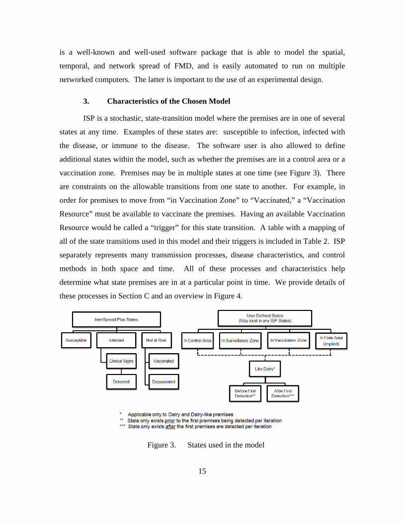
ISP is a stochastic, state-transition model where the premises are in one of several
states at any time. Examples of these states are: susceptible to infection, infected with
the disease, or immune to the disease. The software user is also allowed to define
additional states within the model, such as whether the premises are in a control area or a
vaccination zone. Premises may be in multiple states at one time (see Figure 3). There
are constraints on the allowable transitions from one state to another. For example, in
order for premises to move from “in Vaccination Zone” to “Vaccinated,” a “Vaccination
Resource” must be available to vaccinate the premises. Having an available Vaccination
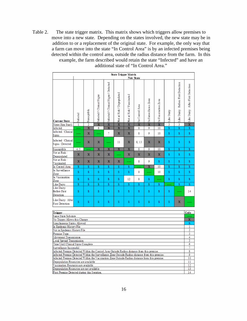
Resource would be called a “trigger” for this state transition. A table with a mapping of
all of the state transitions used in this model and their triggers is included in Table 2. ISP
separately represents many transmission processes, disease characteristics, and control
methods in both space and time. All of these processes and characteristics help
determine what state premises are in at a particular point in time. We provide details of
these processes in Section C and an overview in Figure 4.
Figure 3. States used in the model
16
Table 2. The state trigger matrix. This matrix shows which triggers allow premises to move into a new state. Depending on the states involved, the new state may be in addition to or a replacement of the original state. For example, the only way that a farm can move into the state “In Control Area” is by an infected premises being detected within the control area, outside the radius distance from the farm. In this
example, the farm described would retain the state “Infected” and have an additional state of “In Control Area.”

17
Figure 4. The transmission processes, disease characteristics, and control methods used in our simulation. Notice that some overlap exists between “Transmission Processes” and “Disease Characteristics.” Some
parameters listed under “Movements” are actually characteristics of the disease.
18
B. DATA DESCRIPTION
In this section, we describe the inputs required by the ISP software. Specifically,
we describe the dataset acquired for use in our modeling and our procedure to interpret
and modify it for use by ISP.
1. Description of the Dataset
Although CDFA maintains careful statistics on the location and sizes of
individual farms in California, such information is proprietary and not available to the
public for modeling or analysis. The dataset we use in this thesis is described in Melius,
Robertson, and Hullinger (2006) and includes 25,655 premises locations organized into
the seven columns described below. A sample from the original data is shown in Table 3.
The data were developed from publicly available, county-level, aggregated statistics of
livestock premises provided by the National Agricultural Statistics Service (NASS)
(NASS, 2010). As such, they are an approximation of the locations, sizes, animal types,
and production types of the livestock premises in the state of California. The location
coordinates shown are heterogeneous random locations, selected based on a weighting
scheme using the altitude, flatness, human population, and land use of an area. The size
of the premises is selected by uniformly varying the size according to premises type so
that the average size of each premises type is preserved for each county (Hullinger,
2012). We interpreted the original data as described below:
Premises: a concatenation of the premises type name and the unique
identifier for each premise.
ID: an integer representing a unique identifier for each premise (same
integer as the unique identifier in “Premises”).
Type: a numeric code for the type of premises. Included in the data were
26 of these codes. Premises populated with cattle are assigned codes
between 1 and 99; those populated with swine are assigned codes between
100 and 199; those populated with sheep are assigned codes between
200 and 299; and those populated with goats are assigned codes between
300 and 399. Additionally, code 511 indicates a cattle market and code

19
512 indicates a swine market. We give a complete listing of the type of
codes used in the original data in Table 4.
Size: an integer designating the number of animals on the premises. We
assume that only one type of animal is on each of the premises.
FIPS: the Federal Information Processing Standard (FIPS) code for the
state and county in which the premise is located.
Lat: Latitude of the centroid of the randomized premise location.
Long: Longitude of the centroid of the randomized premise location.
Table 3. A sample of the original data provided by Lawrence Livermore National Laboratory (LLNL)
Premises ID Type Size FIPS Lat Long
Dairy(L):0 0 33
940 6115 39.01372910 -121.5098953
Dairy(L):1 1 33
1,379 6115 39.29288864 -121.5932312
Dairy(L):2 2 33
1,819 6115 39.17738724 -121.4760590
Dairy(L):3 3 33
2,258 6115 39.26313400 -121.5667267
Stocker(S):4
4 61 12 6115 39.10063934 -121.4598846
Stocker(S):5
5 61 15 6115 39.29784775 -121.5664749
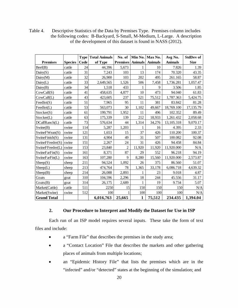
20
Table 4. Descriptive Statistics of the Data by Premises Type. Premises column includes the following codes: B-Backyard, S-Small, M-Medium, L-Large. A description
of the development of this dataset is found in NASS (2012).
Premises SpeciesType Code
Total Animals of Type
No. of Premises
Min No. Animals
Max No. Animals
Avg No. Animals
StdDev of Size
Beef(B) cattle 24 44,396 5,673 1 10 7.826 1.39 Dairy(S) cattle 31 7,243 103 13 174 70.320 43.35 Dairy(M) cattle 32 26,900 103 202 495 261.165 58.87 Dairy(L) cattle 33 2,649,565 1,526 506 7,458 1,736.281 1,057.47 Dairy(B) cattle 34 1,518 433 1 9 3.506 1.85 CowCalf(S) cattle 41 458,635 4,877 10 473 94.040 61.83 CowCalf(L) cattle 43 423,605 237 521 75,512 1,787.363 5,424.75 Feedlot(S) cattle 51 7,965 95 11 381 83.842 81.28 Feedlot(L) cattle 53 563,073 30 1,102 49,667 18,769.100 17,135.79 Stocker(S) cattle 61 199,791 1,952 11 496 102.352 89.49 Stocker(L) cattle 63 175,339 139 212 18,933 1,261.432 2,058.68 DCalfRanch(L) cattle 73 576,634 44 1,314 34,276 13,105.318 9,070.17 Swine(B) swine 114 5,287 1,203 1 16 4.395 2.33 SwineFWean(S) swine 121 1,653 15 37 426 110.200 100.37 SwineFinish(S) swine 131 4,904 49 31 507 100.082 92.08 SwineFFeeder(S) swine 151 2,267 24 31 426 94.458 84.84 SwineFFeeder(L) swine 153 23,840 2 11,920 11,920 11,920.000 N/ASwineFarFin(S) swine 161 8,371 87 29 552 96.218 94.19 SwineFarFin(L) swine 163 107,280 9 8,280 15,560 11,920.000 2,573.87 Sheep(S) sheep 211 94,524 1,092 26 375 86.560 51.07 Sheep(L) sheep 213 474,764 78 1,365 33,178 6,086.718 4,639.32 Sheep(B) sheep 214 26,088 2,893 1 23 9.018 4.87 Goats goat 310 104,596 2,296 18 244 45.556 31.17 Goats(B) goat 314 26,175 2,689 1 19 9.734 5.07 Market(Cattle) cattle 511 2250 15 150 150 150 N/AMarket(Swine) swine 512 100 1 100 100 100 N/AGrand Total 6,016,763 25,665 1 75,512 234.435 1,394.04
2. Our Procedure to Interpret and Modify the Dataset for Use in ISP
Each run of an ISP model requires several inputs. These take the form of text
files and include:
a “Farm File” that describes the premises in the study area;
a “Contact Location” File that describes the markets and other gathering
places of animals from multiple locations;
an “Epidemic History File” that lists the premises which are in the
“infected” and/or “detected” states at the beginning of the simulation; and
21
a “Zone File” listing the boundaries of the area of study in the form of a
series of coordinates forming a polygon.
We describe these inputs in more detail in the following paragraphs.
a. The Farm File
This file is essential to ISP because it describes in detail the area to be
simulated. At a minimum, it must include:
Cartesian coordinates defining where susceptible animals are located (can
be in the form of a centroid or polygon, but here we use the centroid of the
premises);
the number of animals located at each of the premises;
and a premises type for each location (e.g., large dairy, small cattle
feedlot, backyard swine premises).
An arbitrary number of additional columns of user-defined data can also
be included in the farm file to further describe the modeling environment. Next, we
describe the development of our farm file.
In order to develop this farm file, we create a computer program, or
“script,” written in the R Programming Language (R Development Core Team, 2012) to
manipulate the data from the format described above to a text file for import into ISP.
Our first task is to transform the latitude/longitude coordinates provided in our dataset to
integer Cartesian coordinates, as required by ISP. We first add a “zone” column to each
of the premises in the farm file and populate it with an integer between 1 and 6, which
corresponds to the correct California Coordinate System (CCS83) zone to use when
transforming the latitude/longitude columns to northerly/easterly coordinates. The units
of the CCS83 coordinate systems are meters. The correct zone is found by mapping the
FIPS code to the CCS83 zone listed in California Department of Transportation
(Caltrans) (1993). We then use R script, which incorporates the R package “rgdal”
(Stevenson, 2012) as a template to transform the data from latitude/longitude to
northerly/easterly coordinates. We are unable to use the correct zone for each FIPS code
while keeping the correct spatial relationship between the zones. So, we use Zone 3 as

22
the projection for all of the premises locations. From our initial analysis of the distortion
this causes between premises in the far north and far south of the state, it appears that the
incorrect zone usage will not adversely affect our analysis of the simulation.
Next, we split the “Size” column to show the number of each animal
species on each premises. We add five additional columns to indicate species (cattle,
swine, sheep, goat, and other) and initially populate them with zeros. We develop a
mapping table between the “type” column and a “species” column based on the type
described by the “Premises” column in the original data, and use an R script to copy the
number in the “Size” column to the appropriate species column.
Finally, we create another R script to determine the distance between each
of the premises and all other premises in the dataset. This allows us to add six columns
to the data to describe the density of premises and animals within a 3-, 10-, and
20-kilometer (km) radii from each of the premises in the dataset. We will use these
columns to help determine the impact of premises density and animal density on how the
disease spreads within California. These computations are subject to the fact that the
locations given in the dataset are generated by an algorithm and are not the actual
locations of premises. However, we assume that the generated data is representative of
the true locations enough to use these densities in our analysis. We show the
distributions of the densities of premises and animals within the state in Figure 5. We
show similar information in Figures 6 and 7, but display it so that the reader can visualize
where the densely populated areas are located in California. We then show a sample of
the farm file in its final form in Table 5 and describe its columns below.
id: unique identifier (same as original data)
type: numerical code for premises type (same as original data)
FIPS: the FIPS code for the state and county in which the premises are
located (same as original data)
cattle: number of cattle on the premises
swine: number of swine on the premises
sheep: number of sheep on the premises
goat: number of goats on the premises

23
other: number of other animals on the premises (all zeros for this dataset)
premises: description of the type of premises. We develop this column
from the “Premises” column in the original dataset. After splitting the
original column into two columns, a string representing the premises type
name and an integer representing the unique identifier, we remove the
unique identifier column because it is a duplicate of “id.”
premises_3k: number of other premises within a 3-km radius of the given
premises
animal_3k: number of animals (all species) within a 3-km radius of the
given premises
premises_10k: number of other premises within a 3-km radius of the
given premises
animal_10k: number of animals (all species) within a 3-km radius of the
given premises
premises_20k: number of other premises within a 3-km radius of the
given premises
animal_20k: number of animals (all species) within a 3-km radius of the
given premises
xcoord: easterly coordinate (transformed from longitude using a CCS83
Zone 3 projection)
ycoord: northerly coordinate (transformed from latitude using a CCS83
Zone 3 projection)

24
Figure 5. Histograms and descriptive statistics of the within 20-km densities of premises and animals. The histograms show the proportion of premises
(y-axis) that have premises or animal densities of the amount shown along the x-axis. One interesting comparison between these two densities is how differently they are shaped. Premises densities are much more uniformly distributed between densities of 0 and 525 premises and the distribution is bimodal. Animal densities, however, are highly skewed, with almost 50%
of the premises having densities of less than 25,000 animals.
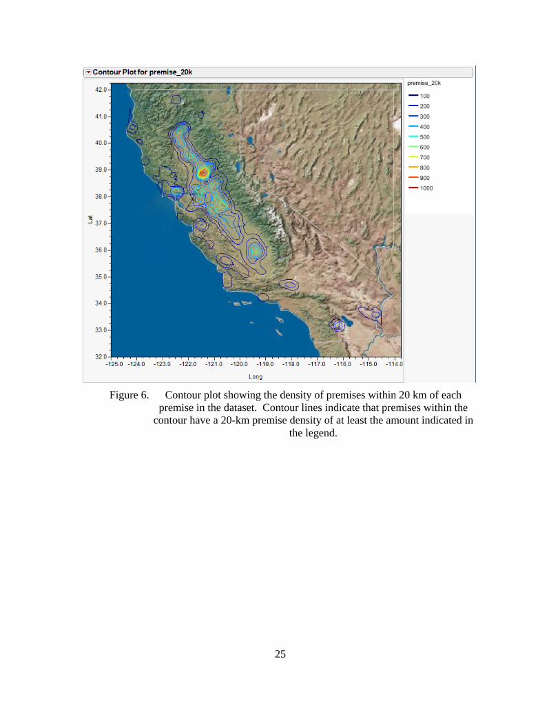
25
Figure 6. Contour plot showing the density of premises within 20 km of each premise in the dataset. Contour lines indicate that premises within the
contour have a 20-km premise density of at least the amount indicated in the legend.
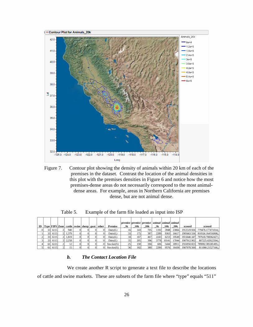
26
Figure 7. Contour plot showing the density of animals within 20 km of each of the premises in the dataset. Contrast the location of the animal densities in this plot with the premises densities in Figure 6 and notice how the most premises-dense areas do not necessarily correspond to the most animal-
dense areas. For example, areas in Northern California are premises dense, but are not animal dense.
Table 5. Example of the farm file loaded as input into ISP
ID Type FIPS Zone cattle swine sheep goat other Premisepremise
_3kpremise
_10kpremise
_20kanimal
_3kanimal_10k
animal_20k xcoord ycoord
0 33 6115 2 940 0 0 0 0 Dairy(L) 16 143 705 1192 3948 23866 1912519.926 779478.177471014;;1 33 6115 2 1,379 0 0 0 0 Dairy(L) 33 175 387 2289 9363 16617 1905663.556 810556.164516908;;2 33 6115 2 1,819 0 0 0 0 Dairy(L) 18 167 467 2243 6213 19549 1915640.347 797618.708362427;;3 33 6115 2 2,258 0 0 0 0 Dairy(L) 35 205 396 3778 10141 17044 1907912.902 807225.65922504;;4 61 6115 2 12 0 0 0 0 Stocker(S) 25 158 594 606 5444 18911 1916950.823 789082.385581495;;5 61 6115 2 15 0 0 0 0 Stocker(S) 36 182 380 2290 9576 16439 1907978.569 811080.21527166;;
b. The Contact Location File
We create another R script to generate a text file to describe the locations
of cattle and swine markets. These are subsets of the farm file where “type” equals “511”
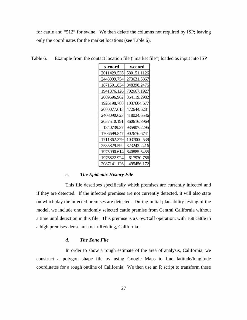
27
for cattle and “512” for swine. We then delete the columns not required by ISP; leaving
only the coordinates for the market locations (see Table 6).
Table 6. Example from the contact location file (“market file”) loaded as input into ISP
x.coord y.coord2011429.535 580151.11262448099.754 273631.58671871501.834 848398.24761941376.126 702667.19272089696.962 354119.29821926198.788 1037604.6772080077.613 472644.62812408090.623 418024.65362057510.191 360616.39691840739.37 935907.2295
1706699.847 902676.67411711862.379 1037000.5392535829.592 323243.24161975990.614 640885.54551976822.924 617930.7862087141.126 495456.172
c. The Epidemic History File
This file describes specifically which premises are currently infected and
if they are detected. If the infected premises are not currently detected, it will also state
on which day the infected premises are detected. During initial plausibility testing of the
model, we include one randomly selected cattle premise from Central California without
a time until detection in this file. This premise is a Cow/Calf operation, with 168 cattle in
a high premises-dense area near Redding, California.
d. The Zone File
In order to show a rough estimate of the area of analysis, California, we
construct a polygon shape file by using Google Maps to find latitude/longitude
coordinates for a rough outline of California. We then use an R script to transform these

28
into CCS83 coordinates that can be used by ISP. Zone 3 is used to transform all
coordinate pairs of the polygon. Figure 8 shows all of the coordinate data included in all
of the ISP input files combined on a single plot.
1600000 1800000 2000000 2200000 2400000 2600000
02
000
004
000
00
60
000
08
000
001
000
000
12
000
00
California Livestock Premises Locations
Easting (m)
No
rthin
g (m
)
PremisesInitially Infected PremisesMarket
Figure 8. California Premises Locations: Shown are the locations of all coordinate data input into ISP for the initial plausibility testing of the model.
C. SIMULATION SOFTWARE PARAMETER AND INITIAL INFECTION SCENARIO DEVELOPMENT
Our first task is to determine a plausible model for how the disease could spread
through California without any controls. This is not to say that this model is predictive of
an actual outbreak of the disease, but that it is plausibly representative of how an

29
outbreak could spread. Then, we develop a model using a generic control strategy and
the same disease spread parameter settings as the uncontrolled model’s settings. In
Chapter III, we describe and compare the results of this plausibility testing.
In order to accomplish the development of these two models, we assembled a
team at the International Data Farming Workshop held March 25–30, 2012, at the Naval
Postgraduate School in Monterey, California to study the problem. The team included
several experts in simulation modeling, computer science, and two veterinarians who are
currently students of the School of Veterinary Medicine at the University of California,
Davis and are studying to attain a Master of Preventive Veterinary Medicine (MPVM)
degree. This team helped us determine the sets of parameters for both the spread of the
disease as well as many of the control parameters shown in Section 4. We divide the
section into six subsections:
Overview of the Control File, which briefly describes the text file used to
input parameter settings into ISP. The control file contains one row
pertaining to each parameter described in the next three topics.
Development of the Model Parameters, which describes the parameters
affecting how the model is run. These include such things as the random
number generator to use and the number of iterations to run the
simulation.
Development of the Disease Spread Parameters, which describes the
network and spatial parameters affecting how the disease is spread from
premises to premises during the simulation.
Development of the Disease Spread Control Parameters, which
describes the strategies and policies to control the spread of the disease as
well as the constraints to those strategies and policies.
Development of Starting Scenarios, which describes the initially
infected premises for eight different scenarios that we model.

30
1. Overview of the Control File
ISP is designed to operate from the command line of a Linux- or Windows-based
single computer, or multiple networked computers, with only one argument specifying
the control file to be used by the software to simulate disease spread. The control file
describes to ISP how the model, disease, and control parameters are used to simulate the
spread of a herd-based disease, both temporally and spatially, through a population. The
development of the control file can be accomplished through the use of a text editor, by a
scripting software language, or by the Control File Editor graphic user interface, which is
packaged with the Windows version of ISP. This text file method enables the modeler to
automate the model to make many different runs of a simulation using many different
scenarios or include different farm, market, or epidemic history files, depending on the
focus of the analysis. We show a sample control file in Appendix B.
2. Development of the Model Parameters
The model parameters section of the control file describes to ISP some basic
information about how the model should be run. In our model, we include the number of
iterations to be completed during the run, the number of time periods to model, a specific
random number generator and seed to use during the run, the maximum infected premises
allowed during the iteration, and a set of user-defined farm states. The parameter settings
and the rationale we use to develop them are given below.
Iteration Count: 100. This is a medium-sized number of runs chosen to
satisfy our computational limitations. The statistical significance from the
experiments is discussed in Chapter V.
Time Period Count: We use 100 days during the experimental design and
40 days during our initial testing. Similar to the iteration count, we
consider 100 days as a medium-sized number that gives us a good idea of
disease behavior without overtaxing processing capability.
Seed: Randomly chosen using a Mersenne Twister generator (Matsumoto
& Nishimura, 1998).
31
Random Generator Name: TRandomMotherOfAll, which is a low-
resolution, low-speed generator with low memory usage (Stevenson,
2012).
Max Infected Farms: 7,700, which is 30% of the total number of premises
in our dataset. We set this limit because we feel that if 30% of premises in
California are infected, the control measures used at the beginning of the
outbreak will be considered ineffective and be replaced with a new
strategy.
User-Defined Farm States
o In Control Area: Premises have been placed in the Control Area.
We trigger this state either when the premises are infected and
detected, or when another premise located at a distance less than or
equal to the designated Control Area outside radius has been
detected.
o In Surveillance Zone: Premises have been placed in the
Surveillance Zone. We trigger this state when another premise
located at a distance less than or equal to the designated
Surveillance Zone outside radius has been detected.
o In Vaccination Zone: Premises have been placed in the
Vaccination Zone. We trigger this state when another premise
located at a distance less than or equal to the designated
Vaccination Zone outside radius has been detected.
o Waiting for Vaccination: The premises have been placed in the
Vaccination Zone and are awaiting resources to become available
to begin vaccination of the animals on the premises.
o Processing Vaccination: Resources have begun vaccination of the
animals on the premises, but are not yet finished with the process.
o Vaccinated: All animals on the premises have been vaccinated.
32
o Waiting for Depopulation: The premises have been infected,
detected, and are awaiting resources to become available to begin
depopulation of the animals on the premises.
o Processing Depopulation: Resources have begun depopulation of
the animals on the premises, but are not yet finished with the
process.
o Depopulated: All animals on the premises have been depopulated.
o likeDairy: Premises have similar surveillance practices to a dairy
facility. These include premises designated as: Dairies (Small-S,
Medium-M, Large-L), Feedlots (S, L), and Dairy Calf Ranches.
o likeDairy before first detection: Premises are designated as
“likeDairy” and no premises have been detected during the current
iteration.
o likeDairy after first detection: Premises are designated as
“likeDairy” and at least one of the premises has been detected
during the current iteration.
o Additional states that were defined, but not used, during this
experiment were Delayed Vaccinated and Delayed Depopulated.
The SetState section of the control file allows the ISP user to designate some
types of premises to a certain modeling state at the beginning of the simulation. We used
this section to designate a modeling state of likeDairy to all Dairy (S, M, L), Feedlot (S,
L), and Dairy Calf Ranches, and we use this modeling state to specify certain surveillance
parameters to use just for dairy and dairy-like premises during the simulation.
3. Development of the Disease-Spread Parameters
ISP has the ability to model many different disease-spread parameters, which
describe the network and spatial disease spread from premises to premises during the
simulation. The sections in the control file describing these parameters are titled:
movement type, route, fixed route, local spread, airborne spread, and infectivity. Of
these, we do not use route and fixed route, which model specific routes between premises

33
(e.g., a milk truck pickup route between several dairy facilities), because data at this level
of detail is not currently available through public sources for California. We also do not
use the airborne spread parameter within ISP. Instead, we assume that varying the local
spread distance parameter will account for the majority of the aerosol spread of the
disease. This assumption is reasonable given that we are modeling a broad range of local
spread distances and the fact that some types/subtypes of the FMD virus do not spread
long distances by aerosol. Additionally, serotype O, which has been responsible for
many recent outbreaks in temperate countries, has shown little tendency for airborne
spread (Stevenson, 2012). We subdivide this section of the thesis by describing the
following sections in the control file:
Movement Type: Network spread of the disease
Local Spread: Spatial spread of the disease over time
Infectivity: Disease characteristics affecting disease spread
a. Movement Type
Even though the zones/areas discussed in Chapter I and Figure 2 seem to
be purely spatial in design, the USDA has recognized that the network spread of FMD
should be considered when designating these zones/areas and recommends the use of
these types of factors in those determinations. Since the virus is easily spread in many
ways, direct and indirect contacts between livestock facilities could happen over greater
distances than are accounted for in a purely spatial design. Direct contact at highly
connected operations, such as livestock markets, occupy a central role in the flow of
animals and should be dealt with differently than other premises in an outbreak area
(Dubé, 2009). Indirect contact, such as by artificial insemination teams or hoof trimmers,
may be higher at different types of operations than others. In a survey of livestock
facilities in California, for example, large swine operations had an over 3,600% higher
mean reported monthly indirect contact rate than small beef farms (Bates et al., 2001).
This seems to be a function of both the size of the herd as well as the species at
the facility.
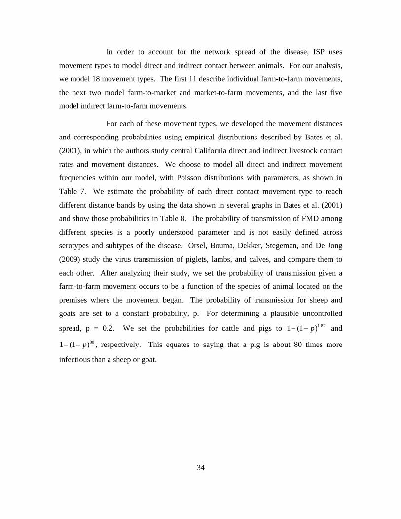
34
In order to account for the network spread of the disease, ISP uses
movement types to model direct and indirect contact between animals. For our analysis,
we model 18 movement types. The first 11 describe individual farm-to-farm movements,
the next two model farm-to-market and market-to-farm movements, and the last five
model indirect farm-to-farm movements.
For each of these movement types, we developed the movement distances
and corresponding probabilities using empirical distributions described by Bates et al.
(2001), in which the authors study central California direct and indirect livestock contact
rates and movement distances. We choose to model all direct and indirect movement
frequencies within our model, with Poisson distributions with parameters, as shown in
Table 7. We estimate the probability of each direct contact movement type to reach
different distance bands by using the data shown in several graphs in Bates et al. (2001)
and show those probabilities in Table 8. The probability of transmission of FMD among
different species is a poorly understood parameter and is not easily defined across
serotypes and subtypes of the disease. Orsel, Bouma, Dekker, Stegeman, and De Jong
(2009) study the virus transmission of piglets, lambs, and calves, and compare them to
each other. After analyzing their study, we set the probability of transmission given a
farm-to-farm movement occurs to be a function of the species of animal located on the
premises where the movement began. The probability of transmission for sheep and
goats are set to a constant probability, p. For determining a plausible uncontrolled
spread, p = 0.2. We set the probabilities for cattle and pigs to 1.821 (1 )p and
801 (1 )p , respectively. This equates to saying that a pig is about 80 times more
infectious than a sheep or goat.

35
Table 7. Shipments from livestock premises. We consider the numeric premises “Type Codes” from our data to be equivalent to the “Facility Types” from Bates et al.
(2001). Green highlighted columns in this table show the data or calculations we add to the authors’ data. The “Actual Mean” column is calculated by multiplying
the “Mean Shipments” by the “% reporting shipments.” The “Average Daily Shipments ” is the “Actual Mean” column divided by 30 to determine a daily rate. This column was used in determining the plausibility of the model. The
similarly calculated “Average Daily Shipments +/– 95% CI” columns are used as high and low limits within the experimental design for their corresponding
movement type rates.
Type CodesPremise
Type No. RespondingNo. Reporting
ShipmentsReporting Shipments
Mean Shipments(Monthly) -95%CI +95%CI Actual Mean
Avg. Daily Shipments
Avg. Daily Shipments
-95%CI
Avg. Daily Shipments+95%CI
24, 34, 114, 214, 314 Backyard 31 29 93.55% 1.7 0 4.2 1.590 0.053 0.000 0.140310 Goat 3 3 100.00% 6.6 0 16.8 6.600 0.220 0.000 0.560211, 213 Sheep 15 15 100.00% 7.9 0 18.8 7.900 0.263 0.000 0.627
Beef51, 61 < 250 52 52 100.00% 0.9 0.5 1.3 0.900 0.030 0.017 0.04353, 63 >= 250 29 28 96.55% 2 0 3 1.931 0.064 0.000 0.100
Dairy31, 32 < 1000 54 52 96.30% 8.2 4.3 12.1 7.896 0.263 0.143 0.403none 1000 - 1999 54 54 100.00% 17.4 12.5 22.3 17.400 0.580 0.417 0.74333 >= 2000 48 48 100.00% 16.4 11.9 20.9 16.400 0.547 0.397 0.697
Calf/heifer41 < 250 10 10 100.00% 0.7 0.3 1.1 0.700 0.023 0.010 0.03743, 73 >= 250 4 4 100.00% 22.4 0 58.8 22.400 0.747 0.000 1.960
Swine121, 131, 151, 161 < 2000 12 11 91.67% 4.8 1.1 8.5 4.400 0.147 0.037 0.283153, 163 >= 2000 5 5 100.00% 20 0.2 39.8 20.000 0.667 0.007 1.327
t = 30
Shipments from the Livestock Premise
Table 8. Movement Distance Probabilities used to model farm-to-farm movements. We estimate the probabilities from the corresponding graphs in Bates et al. (2001).
Again, we consider the numeric premises “Type Codes” from our data to be equivalent to the “Facility Types” from Bates et al. (2001).
Type Code Facility type 19,000 39,000 59,000 79,000 99,000 119,000 139,000 159,000 179,000 24, 34, 114, 214, 314 Backyard 0.615 0.110 0.025 0.060 0.010 0.035 0.010 0.000 0.135211, 213, 310 Goat/Sheep 0.365 0.160 0.090 0.035 0.010 0.000 0.015 0.025 0.30051, 53, 61, 63 Beef 0.390 0.220 0.125 0.055 0.025 0.010 0.020 0.015 0.14031, 32, 33 Dairy 0.570 0.255 0.035 0.010 0.005 0.010 0.005 0.005 0.10541, 43, 73 Calf/heifer 0.410 0.145 0.205 0.000 0.000 0.000 0.020 0.000 0.220121, 131, 151, 153, 161, 163 Swine 0.315 0.290 0.020 0.050 0.120 0.045 0.015 0.000 0.145
Average Probability for Specified Distance Travelled To/From a Livestock Premise(Distance in Meters)
We continue to use Bates et al. (2001) as a basis to develop the parameters
for indirect contact movements. We calculate monthly indirect contact movement rates
by subtracting the employee and friend columns from the total mean number of monthly
indirect contacts shown in the authors’ data, in order to model only higher risk, indirect
contact. We assume employees and friends are lower risk due to their limited exposure to

36
animals on other livestock premises on a single day; however, this may not be true given
the number of farm employees who may have more than one job or keep livestock at
home. We then divide the monthly rates by 30 to determine the daily rates and multiply
this daily rate by a probability that the indirect contact moves to another susceptible
premises. Finally, we combine similar probabilities for efficiency’s sake within the ISP
(see Table 9). We then estimate the probabilities for different movement distances for
indirect contacts from another table by the authors (see Table 10). The probabilities of
transmission use the same function as the direct contact movements given above.
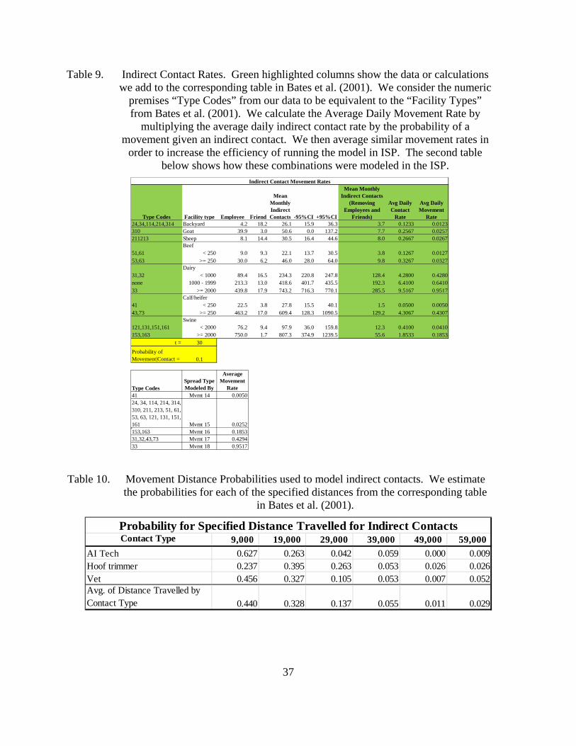
37
Table 9. Indirect Contact Rates. Green highlighted columns show the data or calculations we add to the corresponding table in Bates et al. (2001). We consider the numeric
premises “Type Codes” from our data to be equivalent to the “Facility Types” from Bates et al. (2001). We calculate the Average Daily Movement Rate by
multiplying the average daily indirect contact rate by the probability of a movement given an indirect contact. We then average similar movement rates in
order to increase the efficiency of running the model in ISP. The second table below shows how these combinations were modeled in the ISP.
Type Codes Facility type Employee Friend
Mean Monthly Indirect Contacts -95%CI +95%CI
Mean Monthly Indirect Contacts
(Removing Employees and
Friends)
Avg Daily Contact
Rate
Avg Daily Movement
Rate24,34,114,214,314 Backyard 4.2 18.2 26.1 15.9 36.3 3.7 0.1233 0.0123310 Goat 39.9 3.0 50.6 0.0 137.2 7.7 0.2567 0.0257211213 Sheep 8.1 14.4 30.5 16.4 44.6 8.0 0.2667 0.0267
Beef51,61 < 250 9.0 9.3 22.1 13.7 30.5 3.8 0.1267 0.012753,63 >= 250 30.0 6.2 46.0 28.0 64.0 9.8 0.3267 0.0327
Dairy31,32 < 1000 89.4 16.5 234.3 220.8 247.8 128.4 4.2800 0.4280none 1000 - 1999 213.3 13.0 418.6 401.7 435.5 192.3 6.4100 0.641033 >= 2000 439.8 17.9 743.2 716.3 770.1 285.5 9.5167 0.9517
Calf/heifer41 < 250 22.5 3.8 27.8 15.5 40.1 1.5 0.0500 0.005043,73 >= 250 463.2 17.0 609.4 128.3 1090.5 129.2 4.3067 0.4307
Swine121,131,151,161 < 2000 76.2 9.4 97.9 36.0 159.8 12.3 0.4100 0.0410153,163 >= 2000 750.0 1.7 807.3 374.9 1239.5 55.6 1.8533 0.1853
t = 30
Probability of Movement|Contact = 0.1
Type CodesSpread Type Modeled By
Average Movement
Rate41 Mvmt 14 0.005024, 34, 114, 214, 314, 310, 211, 213, 51, 61, 53, 63, 121, 131, 151, 161 Mvmt 15 0.0252153,163 Mvmt 16 0.185331,32,43,73 Mvmt 17 0.429433 Mvmt 18 0.9517
Indirect Contact Movement Rates
Table 10. Movement Distance Probabilities used to model indirect contacts. We estimate the probabilities for each of the specified distances from the corresponding table
in Bates et al. (2001).
Contact Type 9,000 19,000 29,000 39,000 49,000 59,000
AI Tech 0.627 0.263 0.042 0.059 0.000 0.009Hoof trimmer 0.237 0.395 0.263 0.053 0.026 0.026Vet 0.456 0.327 0.105 0.053 0.007 0.052Avg. of Distance Travelled by Contact Type 0.440 0.328 0.137 0.055 0.011 0.029
Probability for Specified Distance Travelled for Indirect Contacts
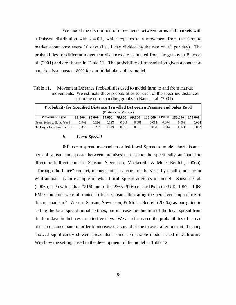
38
We model the distribution of movements between farms and markets with
a Poisson distribution with , which equates to a movement from the farm to
market about once every 10 days (i.e., 1 day divided by the rate of 0.1 per day). The
probabilities for different movement distances are estimated from the graphs in Bates et
al. (2001) and are shown in Table 11. The probability of transmission given a contact at
a market is a constant 80% for our initial plausibility model.
Table 11. Movement Distance Probabilities used to model farm to and from market movements. We estimate these probabilities for each of the specified distances
from the corresponding graphs in Bates et al. (2001).
Movement Type 19,000 39,000 59,000 79,000 99,000 119,000 139000 159,000 179,000
From Seller to Sales Yard 0.546 0.216 0.167 0.018 0.005 0.014 0.004 0.006 0.024To Buyer from Sales Yard 0.383 0.202 0.119 0.061 0.013 0.069 0.04 0.021 0.092
Probability for Specified Distance Travelled Between a Premise and Sales Yard(Distance in Meters)
b. Local Spread
ISP uses a spread mechanism called Local Spread to model short distance
aerosol spread and spread between premises that cannot be specifically attributed to
direct or indirect contact (Sanson, Stevenson, Mackereth, & Moles-Benfell, 2006b).
“Through the fence” contact, or mechanical carriage of the virus by small domestic or
wild animals, is an example of what Local Spread attempts to model. Sanson et al.
(2006b, p. 3) writes that, “2160 out of the 2365 (91%) of the IPs in the U.K. 1967 – 1968
FMD epidemic were attributed to local spread, illustrating the perceived importance of
this mechanism.” We use Sanson, Stevenson, & Moles-Benfell (2006a) as our guide to
setting the local spread initial settings, but increase the duration of the local spread from
the four days in their research to five days. We also increased the probabilities of spread
at each distance band in order to increase the spread of the disease after our initial testing
showed significantly slower spread than some comparable models used in California.
We show the settings used in the development of the model in Table 12.
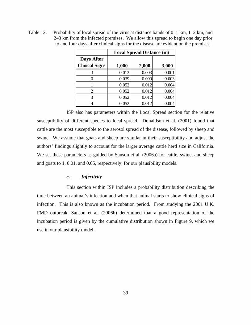
39
Table 12. Probability of local spread of the virus at distance bands of 0–1 km, 1–2 km, and 2–3 km from the infected premises. We allow this spread to begin one day prior to and four days after clinical signs for the disease are evident on the premises.
Days After Clinical Signs 1,000 2,000 3,000
-1 0.013 0.003 0.0010 0.039 0.009 0.0031 0.052 0.012 0.0042 0.052 0.012 0.0043 0.052 0.012 0.0044 0.052 0.012 0.004
Local Spread Distance (m)
ISP also has parameters within the Local Spread section for the relative
susceptibility of different species to local spread. Donaldson et al. (2001) found that
cattle are the most susceptible to the aerosol spread of the disease, followed by sheep and
swine. We assume that goats and sheep are similar in their susceptibility and adjust the
authors’ findings slightly to account for the larger average cattle herd size in California.
We set these parameters as guided by Sanson et al. (2006a) for cattle, swine, and sheep
and goats to 1, 0.01, and 0.05, respectively, for our plausibility models.
c. Infectivity
This section within ISP includes a probability distribution describing the
time between an animal’s infection and when that animal starts to show clinical signs of
infection. This is also known as the incubation period. From studying the 2001 U.K.
FMD outbreak, Sanson et al. (2006b) determined that a good representation of the
incubation period is given by the cumulative distribution shown in Figure 9, which we
use in our plausibility model.

40
Figure 9. Cumulative distribution describing probabilities associated with the time between animal infection and the onset of clinical signs of the disease
(Sanson, 2006b). All species use the same distribution.
The other parameter we used in the Infectivity section describes the
variation of herd infectiousness over time. This parameter is multiplied by the
probability of transmission parameters in the other sections to specify an overall
probability of transmission. Sanson et al. (2006b) estimated this parameter by utilizing a
Delphi conference of FMD experts. The participants at this conference determined that
this parameter could be represented by a linear function decreasing from the 16th day
after herd infection to the 33rd day after herd infection at a rate of 0.059.
4. Development of the Disease-Spread Control Parameters
Similar to Section 3, we wish to first check that our controlled spread model is
plausible, so we initially set it up with mean or most likely parameter settings and test it
to ensure that the disease control parameters are having an effect on the spread of the
disease. ISP contains eight sections that model the control measures that may be
undertaken to combat an outbreak of FMD. We do not model a statewide movement
standstill, since this response is not specifically included in the CDFA FMD response
plans (CDFA, 2006). The seven sections we use are listed below and described in the
following paragraphs.

41
Zones: apply to premises based on its modeling state and proximity to
explicit boundaries or other premises
Surveillance: models the detection of an infected premises
Resources: applies constraints to the amount of depopulation or
vaccination controls
Depopulation: describes the depopulation strategy used by the model
Vaccination: describes the vaccination strategy used by the model
Tracing: models the detection of movements of the disease on or off a
premise
Movement Restrictions: describes how different movement types are
restricted upon the first detection of an infected premise during the
simulation
a. Zones
Similar to how ISP applies different modeling states to specific premises
during the course of a simulation, ISP applies “Zones” to specific premises based on their
geographic location. A user can define these zones explicitly using coordinate polygons
or radially around a specific premise, in a specific modeling state. The user may also
specify specific start and stop times for these zones, or have them triggered by a premise
being assigned a specific modeling state. For our model, we use two explicit zones and
three radial zones and describe them below:
ZoneCalifornia: Explicit zone used to describe the boundaries of the
modeling area, which is the state of California. We start this zone at the
simulation start and keep it active for the entire simulation. This zone
contains all premises in our dataset.
Zone_ControlArea: Radial zone used to represent the Control Area and to
define an area within a certain distance from a detected premise. If a
premise is located in this zone, ISP will assign a model state of
in_control_area and apply certain movement restrictions and surveillance
methods to that premise as described below. Control area zones will be
42
active for the entire length of the simulation, beginning when the first
premises are detected with the disease. The outside radius used for initial
plausibility testing will be 10 km, which is the minimum radius
recommended by the USDA for a control area (USDA, 2011).
Zone_Vaccinate: Radial zone used to represent a Vaccination zone and to
define an area within a certain distance from a detected premise. If a
premise is located in this zone, ISP will assign a model state of
in_vacc_zone and the premise will be added to a vaccination premises list,
which will be described in the Vaccination paragraph below. Vaccination
zones will be active for the entire length of the simulation, beginning
when the first premises are detected with the disease. The USDA does not
have a recommended radius for a vaccination zone, so we use 10 km as
the outside radius for initial plausibility testing of the model.
Zone_Surv: Radial zone used to represent the Surveillance Zone and to
define an area within a certain distance from a detected premise. For
premises located in this zone, ISP will assign a model state of
in_surv_zone unless those premises are already in a control area. ISP will
then apply certain movement restrictions and surveillance methods to
those premises as described below. Surveillance zones will be active for
the entire length of the simulation beginning when the first premises are
detected with the disease. The outside radius used for initial plausibility
testing will be 25 km, which is 5 km larger than the minimum radius
recommended by the USDA for a control area (USDA, 2011).
Zone_likeDairy: Explicit zone with the same boundaries as
ZoneCalifornia above, but used to represent premises with a likeDairy
modeling state. If premises are located in this zone, ISP applies certain
movement restrictions and surveillance methods to those premises as
described below. The likeDairy zone will be active for the entire length of
the simulation.

43
b. Surveillance
ISP models the detection of infected premises using the Surveillance
section of the control file. When a premises changes from an infected state to a detected
state, authorities would assumedly impose some types of control measures to limit the
disease spread. ISP uses two parameters to determine the likelihood of detection. The
proportion of premises that participate in a surveillance type is called the selection
probability, whereas the probability of an infected premise being detected, given that it is
visited by a surveillance team, is called the detection probability. The detection
probability can also be specified for each species modeled as desired by the user. We use
Sanson et al. (2006b) and Hullinger (2012) as guides to these probabilities for the
plausibility test of our model. Additionally, ISP models three rates within each type of
surveillance:
Visit delay, which is the rate at which the surveillance is delayed to a
premise given it is selected for certain surveillance type;
Visit frequency, which is the rate between visits while the premise is still
on a surveillance list; and
Delay to detection, which is the amount of time that passes between when
a successful visit occurred on an infected premise and when that premise
will be given the detected model state.
We show the surveillance parameter settings for our model in Table 13.
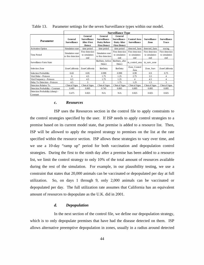
44
Table 13. Parameter settings for the seven Surveillance types within our model.
ParameterGeneral
Surveillance
General Surveillance After First
Detect
General Surveillance - Dairy Before First Detect
General Surveillance - Dairy After First Detect
Control Area Surveillance
Surveillance Zone
Surveillance Trace
Activation Option Simulation start time period time period time period detected_farm detected_farm tracing
Time PeriodSimulation start to first detection
First detection to simulation
end
Simulation start to first detection
First detection to simulation
end
First detection to simulation
end
First detection to simulation
end
First detection to simulation
end
Surveillance Farm StatelikeDairy_before
DetectlikeDairy_after
Detectin_control_area in_surv_zone
Selection Zone ZoneCalifornia ZoneCalifornia likeDairy likeDairyZone_Control
AreaZone_Surv ZoneCalifornia
Selection Probability 0.65 0.85 0.999 0.999 0.99 0.9 0.75Visit Delay - Poisson 6 4.5 1.75 1.25 2.75 3.5 4Visit Frequency - Poisson 6.5 4.5 1.75 1.25 4 4.5 4Delay To Detection - Poisson 4.5 3 3 1.75 1.25 1.5 3Detection Relative To Clinical Signs Clinical Signs Clinical Signs Clinical Signs Clinical Signs Clinical Signs Clinical SignsDetection Probability - Constant 0.495 0.895 0.745 0.895 0.895 0.895 0.895Detection Probability (sheep) - Constant
0.475 0.825 N/A N/A 0.825 0.825 0.825
Surveillance Type
c. Resources
ISP uses the Resources section in the control file to apply constraints to
the control strategies specified by the user. If ISP needs to apply control strategies to a
premise based on its current model state, that premise is added to a resource list. Then,
ISP will be allowed to apply the required strategy to premises on the list at the rate
specified within the resource section. ISP allows these strategies to vary over time, and
we use a 10-day “ramp up” period for both vaccination and depopulation control
strategies. During the first to the ninth day after a premise has been added to a resource
list, we limit the control strategy to only 10% of the total amount of resources available
during the rest of the simulation. For example, in our plausibility testing, we use a
constraint that states that 20,000 animals can be vaccinated or depopulated per day at full
utilization. So, on days 1 through 9, only 2,000 animals can be vaccinated or
depopulated per day. The full utilization rate assumes that California has an equivalent
amount of resources to depopulate as the U.K. did in 2001.
d. Depopulation
In the next section of the control file, we define our depopulation strategy,
which is to only depopulate premises that have had the disease detected on them. ISP
allows alternative preemptive depopulation in zones, usually in a radius around detected
45
premises, but we chose not to model this control measure because of our understanding
of the current views in California to such a practice (Hullinger, 2012). The parameter
settings we use are to activate a depopulation action upon ISP assigning a premise to the
modeling state of “detected” and the action will only be applied to that particular
premise. We will constrain this action using the depopulation resource described above.
e. Vaccination
Our vaccination strategy for the plausibility test is to vaccinate likeDairy
premises that are assigned to the vaccination zone. Vaccinations are completed from the
outside to the inside of a radial vaccination zone and are constrained by the resources
described in the “Resources” paragraph above. Once a premise is vaccinated, its
probability of infection by another premise is reduced, based on a user-defined lookup
table. This table defines the proportion of animals on the premise that are not immune to
infection at a given point in time. We use conservative estimates of this proportion,
which we derived from Doel et al. (1994). The authors examined the rate of development
of immunity in several FMD susceptible species, including cattle, and found that all of
the cattle they tested were immune four days after vaccination. However, they also cite
other studies that indicated that this result may be optimistic. Our table states that 10% of
the animals on the premises are not immune after four days and 0.5% are not immune
after 15 days. The effect of this proportion is that ISP multiplies the probability of
transmission by this proportion to determine a new overall probability of transmission.
For example, if a certain infected premise attempted to spread the disease to other
premises that were in their fifth day after vaccination, ISP would multiply the calculated
probability of transmission (e.g., 0.5) by 0.1, the number in the table, to reach an overall
probability of transmission of 0.05.
f. Tracing
This is the attempt to find contacts that have been made onto or off of a
particular detected premise. ISP can model both types of tracing, backward and forward.
Backward tracing involves interviewing the staff of a certain detected premise to
determine what direct and indirect contacts were possible between the start of the

46
outbreak and the presumed date of the premise’s infection, which is based on the
observation of the clinical signs of the disease. The goal of backward tracing is to
determine what premises could have infected the detected premise and then to apply
certain controls or surveillance to the possibly infected premise. In contrast, the goal of
forward tracing is to determine what other premises that the detected premises could have
infected since the presumed date of infection. This is accomplished in the same manner
as backward tracing, by personal interview of the staff of the detected premise.
The ISP user can define tracing parameters for forward and backward
tracing for each individual movement type or define them globally for all movement
types. We apply the settings globally within our model. The tracing parameters available
include: when the tracing action will begin, the probability that a movement is forgotten,
and the rate at which tracing interviews are accomplished. We use all of these parameters
as described below:
Time period to start tracing: We begin tracing operations two days after
the first detection and continue them through the entire simulation.
Probability the movement is forgotten: We use a setting of 42.5% of
movements will be forgotten.
Tracing delay: We use a Poisson distribution with a mean rate of delay of
3.75 for this setting. This equates to having to an average time until
tracing is complete of almost four days.
g. Movement Restrictions
ISP reduces the rate for each movement type after the first infected
premise is detected using the movement restriction parameters within the control file.
For our model, we define three movement restrictions. For all movement types with a
source or destination premise in a control area, the probability that the movement will not
occur is set to 92%. For all movement types with a source or destination premise in a
surveillance zone, the probability that the movement will not occur is set to 84.5%. We
added an additional movement restriction on all to or from market movement within
California in order to test that control strategy. This restriction is turned on or off by

47
setting the probability that the movement will not occur to either 0% or 99%, depending
on the strategy used. For our plausibility testing, this probability was set to 0%, meaning
that only markets in a control area or surveillance zone are affected by a movement
restriction.
5. Development of Starting Scenarios
As mentioned earlier, the majority of the studies conducted on the spread of FMD
in California have been limited to the Central Valley of the state, where the majority of
the large livestock premises are located. We wish to broaden that scope by starting
outbreaks of the disease randomly chosen from all premises in California if they meet
certain conditions. The conditions we choose are based on the suspected sources of FMD
outbreaks of modern livestock countries as well as expert opinion (Hullinger, 2012 &
Stevenson, 2012). We show the scenarios we model in Table 14.

48
Table 14. Description, methodology, and rationale behind the scenarios we model.
Scenario Description Methodology Rationale
Southern Border
Randomly infect five cattle facilities along the southern border of California to represent spread from a Mexican FMD outbreak.
If [(Latitude <= 33 or Longitude >= -115) And number of Cattle on Farm > 10], then eligible for selection. Randomly selected 5 initially infected premise from eligible list.
Bulgaria, 2011. Index case was near the Turkish border and a feral pig was antemordem diagnosed with FMD. Turkey had an FMD outbreak occuring at the time.
MarketRandomly infect one market to represent spread from direct or indirect contact.
If Type = 511 OR 512, then eligible for selection. Randomly select 1 to be initially infected premise.
Markets are known to be supernodes in the spread of FMD. The source of infection to the market could have been a person involved in the livestock industry who had recently returned from travel to a country with a current FMD outbreak.
San Francisco Port
Randomly infect one swine facility near San Francisco to represent illegal import of feed for swine (as in UK outbreak of 2001).
If [(37.25 < Latitude <= 38.25 And Longitude < -121.75) And number of Swine on Farm > 10], then eligible for selection. Randomly selected 1 initially infected premise from the eligible list.
LA Port
Randomly infect one swine facility near Los Angeles to represent illegal import of feed for swine (as in UK outbreak of 2001).
If [(33.2 < Latitude <= 34.2 And Longitude < -117) And number of Swine on Farm > 10], then eligible for selection. Randomly selected 1 initially infected premise from the eligible list.
High Animal DensityRandomly infect one cattle facility in an area in the 90th percentile or higher of animal-dense locations.
If [(Number of Animals within 10k > 47779 (90th Percentile)) And (Latitude > 34) And number of Cattle on Farm > 10)], then eligible for selection. Randomly selected 1 initially infected premise from the eligible list.
Conducted in order to compare our model to other models of FMD in California, most of which are in high animal dense areas. Also, this is the most likely area to be infected by an terrorist organization.
Low Animal DensityRandomly infect one cattle facility in an area in the 10th percentile or lower of animal-dense locations.
If [(Number of Animals within 10k < 647 (10th Percentile)) And (Latitude > 34) And number of Cattle on Farm > 10)], then eligible for selection. Randomly selected 1 initially infected premise from the eligible list.
Conducted to contrast with the High Animal Density Scenario.
High Premise DensityRandomly infect one cattle facility in an area in the 90th percentile or higher of premise-dense locations.
If [(Number of Farms within 10k > 185 (90th Percentile)) And (Latitude > 34) And number of Cattle on Farm > 10)], then eligible for selection. Randomly selected 1 initially infected premise from the eligible list.
Conducted in order to determine how ISP reacts to high premise dense areas in comparison with high animal dense areas. This may also indicate how the disease could spread through Northern California, which is a geographic area which has not been studied as much as other areas of the state.
Low Premise DensityRandomly infect one cattle facility in an area in the 10th percentile or lower of premise-dense locations.
If [(Number of Farms within 10k < 12 (10th Percentile)) And (Latitude > 34) And number of Cattle on Farm > 10)], then eligible for selection. Randomly selected 1 initially infected premise from the eligible list.
Conducted to contrast with the High Premise Density Scenario.
Swine infected by feeding on illegally imported meat were the probable sources of infection in Taiwan (1997), the UK (2001), and South Korea (2011)
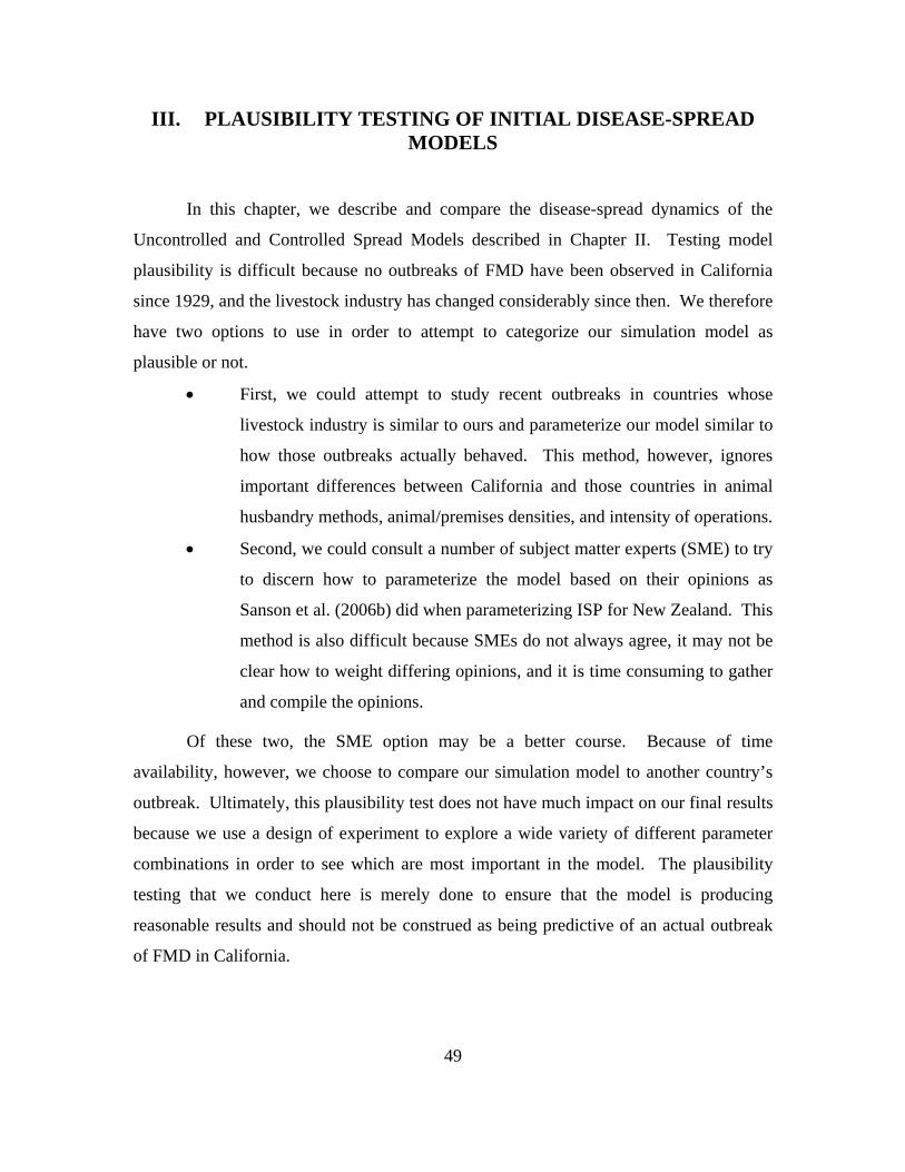
49
III. PLAUSIBILITY TESTING OF INITIAL DISEASE-SPREAD MODELS
In this chapter, we describe and compare the disease-spread dynamics of the
Uncontrolled and Controlled Spread Models described in Chapter II. Testing model
plausibility is difficult because no outbreaks of FMD have been observed in California
since 1929, and the livestock industry has changed considerably since then. We therefore
have two options to use in order to attempt to categorize our simulation model as
plausible or not.
First, we could attempt to study recent outbreaks in countries whose
livestock industry is similar to ours and parameterize our model similar to
how those outbreaks actually behaved. This method, however, ignores
important differences between California and those countries in animal
husbandry methods, animal/premises densities, and intensity of operations.
Second, we could consult a number of subject matter experts (SME) to try
to discern how to parameterize the model based on their opinions as
Sanson et al. (2006b) did when parameterizing ISP for New Zealand. This
method is also difficult because SMEs do not always agree, it may not be
clear how to weight differing opinions, and it is time consuming to gather
and compile the opinions.
Of these two, the SME option may be a better course. Because of time
availability, however, we choose to compare our simulation model to another country’s
outbreak. Ultimately, this plausibility test does not have much impact on our final results
because we use a design of experiment to explore a wide variety of different parameter
combinations in order to see which are most important in the model. The plausibility
testing that we conduct here is merely done to ensure that the model is producing
reasonable results and should not be construed as being predictive of an actual outbreak
of FMD in California.
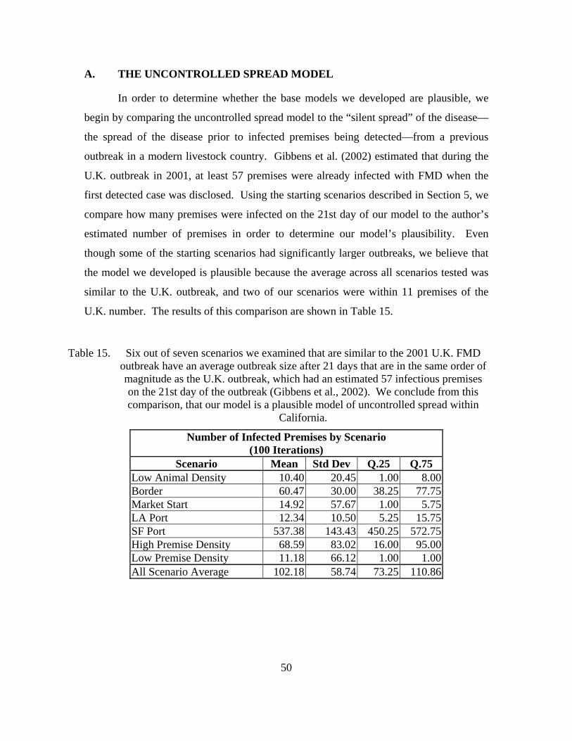
50
A. THE UNCONTROLLED SPREAD MODEL
In order to determine whether the base models we developed are plausible, we
begin by comparing the uncontrolled spread model to the “silent spread” of the disease—
the spread of the disease prior to infected premises being detected—from a previous
outbreak in a modern livestock country. Gibbens et al. (2002) estimated that during the
U.K. outbreak in 2001, at least 57 premises were already infected with FMD when the
first detected case was disclosed. Using the starting scenarios described in Section 5, we
compare how many premises were infected on the 21st day of our model to the author’s
estimated number of premises in order to determine our model’s plausibility. Even
though some of the starting scenarios had significantly larger outbreaks, we believe that
the model we developed is plausible because the average across all scenarios tested was
similar to the U.K. outbreak, and two of our scenarios were within 11 premises of the
U.K. number. The results of this comparison are shown in Table 15.
Table 15. Six out of seven scenarios we examined that are similar to the 2001 U.K. FMD outbreak have an average outbreak size after 21 days that are in the same order of magnitude as the U.K. outbreak, which had an estimated 57 infectious premises on the 21st day of the outbreak (Gibbens et al., 2002). We conclude from this comparison, that our model is a plausible model of uncontrolled spread within
California.
Number of Infected Premises by Scenario (100 Iterations)
Scenario Mean Std Dev Q.25 Q.75 Low Animal Density 10.40 20.45 1.00 8.00 Border 60.47 30.00 38.25 77.75 Market Start 14.92 57.67 1.00 5.75 LA Port 12.34 10.50 5.25 15.75 SF Port 537.38 143.43 450.25 572.75 High Premise Density 68.59 83.02 16.00 95.00 Low Premise Density 11.18 66.12 1.00 1.00 All Scenario Average 102.18 58.74 73.25 110.86
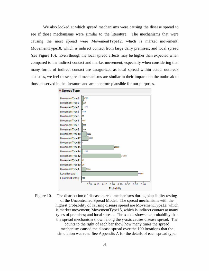
51
We also looked at which spread mechanisms were causing the disease spread to
see if those mechanisms were similar to the literature. The mechanisms that were
causing the most spread were MovementType12, which is market movement;
MovementType18, which is indirect contact from large dairy premises; and local spread
(see Figure 10). Even though the local spread effects may be higher than expected when
compared to the indirect contact and market movement, especially when considering that
many forms of indirect contact are catagorized as local spread within actual outbreak
statistics, we feel these spread mechanisms are similar in their impacts on the outbreak to
those observed in the literature and are therefore plausible for our purposes.
Figure 10. The distribution of disease-spread mechanisms during plausibility testing of the Uncontrolled Spread Model. The spread mechanisms with the
highest probability of causing disease spread are MovementType12, which is market movement; MovementType15, which is indirect contact at many types of premises; and local spread. The x-axis shows the probability that the spread mechanism shown along the y-axis causes disease spread. The
counts to the right of each bar show how many times the spread mechanism caused the disease spread over the 100 iterations that the
simulation was run. See Appendix A for the details of each spread type.
52
B. THE CONTROLLED SPREAD MODEL
Determining the plausibility of the controlled spread model is more difficult than
the uncontrolled model, since the controls used are unique to what we believe are “most
likely” control scenarios for the United States and, as such, are not comparable to
outbreaks in other countries. In order to determine plausibility, we simply observe how
the uncontrolled spread model is affected by the same set of controls over all starting
scenarios to ensure that the outputs are reasonable. We found that the control parameter
settings affected the uncontrolled spread model predictably for all scenarios. An example
showing the spread comparison between models, using the High Premises Density
scenario, is shown in Figure 11, and the distribution of spread mechanisms is shown in
Figure 12.
Figure 11. Comparison of Plausibility Models: Uncontrolled Spread vs. Controlled Spread. By observing the infected premises curve for both the
uncontrolled and the controlled spread on a log scale, we can see the effect of detecting an infected premise. Here, the minimum detection time over
100 simulation iterations was two days, but the effect of the detection begins on Day 4, based on the length of time needed to apply controls.
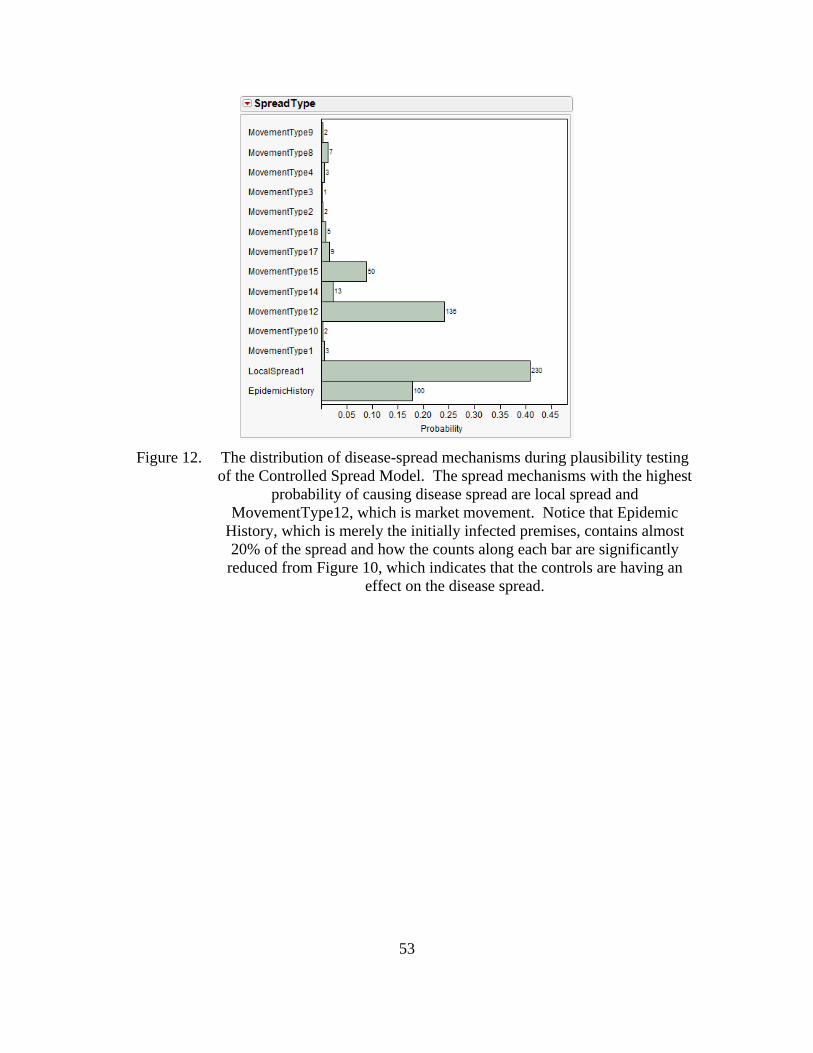
53
Figure 12. The distribution of disease-spread mechanisms during plausibility testing of the Controlled Spread Model. The spread mechanisms with the highest
probability of causing disease spread are local spread and MovementType12, which is market movement. Notice that Epidemic
History, which is merely the initially infected premises, contains almost 20% of the spread and how the counts along each bar are significantly reduced from Figure 10, which indicates that the controls are having an
effect on the disease spread.

54
THIS PAGE INTENTIONALLY LEFT BLANK

55
IV. SIMULATION EXPERIMENTAL DESIGN
Because intentionally introducing the virus into a large livestock population is not
a viable method for scientific inquiry, FMD is generally studied in one of three ways:
Live virus infection and study of a limited quantity of susceptible animals
to determine virus and vaccine characteristics;
Statistical studies of past or current outbreaks to study how diseases have
spread through populations, given the characteristics of the study area and
virus type/subtype; and
Simulation modeling to attempt to predict the characteristics of future
outbreaks.
We intend to use the research completed by others in the first two ways to inform
our research of the third way—simulation modeling. We do this by designing an
efficient experimental design that varies the parameters of the simulation in order to find
response strategies that are robust to those variations. The next section explains how this
was done by giving an overview of why we use an experimental design in general, and
then how we implemented our design specifically.
A. WHY WE USE AN EXPERIMENTAL DESIGN
In Chapter II, Section A, we described some of the objectives of simulation
modeling of a disease. There exists significant uncertainty in the way that a disease
spreads through a population; the manner in which the first premises are infected; and
what policies, technologies, and logistical constraints we may have in our attempts to
control the disease. In order to study how the disease may spread and to find control
measures that are robust to these uncertainties, we run the simulation many times using a
variety of simulation parameter settings, initial infection scenarios, and control strategies.
With 73 factors considered in our model, conducting a full-factorial design—one that
tries every combination of factors—is computationally intractable. Even by making
every factor binary, having only a high and low setting, it would require 273 simulation

56
runs. Instead, we conduct this experiment in an intelligent way in order to maximize our
insights and conclusions. So, we use an efficient experimental design. As Sanchez
(2008, p. 73) states,
…for those interested in exploring the I/O (Input/Output) behavior of their simulation model, efficient experimental design has a much higher payoff at a much lower cost. A well-designed experiment allows the analyst to examine many more factors than would otherwise be possible, while providing insights that cannot be gleaned from trial-and-error approaches or by sampling factors one at a time.
An experimental design is a matrix in which every row represents one simulation
run, called a design point, and every column represents a certain parameter, called a
factor. In our case, the factors include the different ways the disease could behave, the
environment in which the disease starts and spreads, and the controls we impose to stop
that spread. Examples of the factors we look at in the experimental design include: the
rate at which animals start to show clinical signs of FMD, the probability of an animal
being moved some distance and spreading the disease, and how often animals are
observed for signs of the disease. Our goal is to then test the factors at many different
settings, called levels, in an efficient way that allows us to see the factor levels’ effects on
the spread of the disease without undue strain on our computational resources.
Many experimental designs for simulations exist in the literature and several have
been designed at the Naval Postgraduate School’s Simulation Experiments and Efficient
Design (SEED) Center. Most of these designs are based on nearly orthogonal Latin
hypercube (NOLH) designs and may be crossed with a traditional factorial design to
make a mixed design (Cioppa & Lucas, 2007). NOLH designs have good qualities in
that they are “space-filling” and have minimal pairwise correlations between factors. The
former is beneficial because it explores the entire sample space and the latter because it
ensures that the metamodel developed from the design will indicate factor coefficients
very similar to the true, unknown, coefficients—even in the presence or absence of other
more significant factors. In other words, even if the factors we include in our experiment
are not the most significant factors impacting the simulation output, the metamodel is still
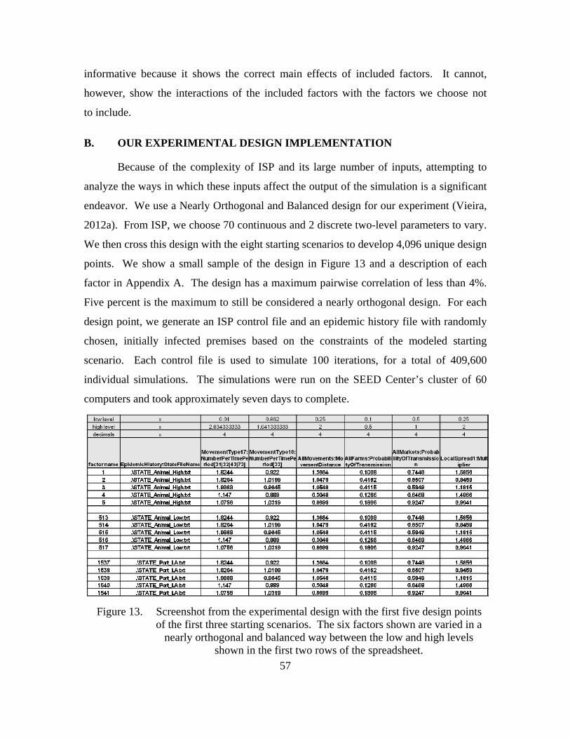
57
informative because it shows the correct main effects of included factors. It cannot,
however, show the interactions of the included factors with the factors we choose not
to include.
B. OUR EXPERIMENTAL DESIGN IMPLEMENTATION
Because of the complexity of ISP and its large number of inputs, attempting to
analyze the ways in which these inputs affect the output of the simulation is a significant
endeavor. We use a Nearly Orthogonal and Balanced design for our experiment (Vieira,
2012a). From ISP, we choose 70 continuous and 2 discrete two-level parameters to vary.
We then cross this design with the eight starting scenarios to develop 4,096 unique design
points. We show a small sample of the design in Figure 13 and a description of each
factor in Appendix A. The design has a maximum pairwise correlation of less than 4%.
Five percent is the maximum to still be considered a nearly orthogonal design. For each
design point, we generate an ISP control file and an epidemic history file with randomly
chosen, initially infected premises based on the constraints of the modeled starting
scenario. Each control file is used to simulate 100 iterations, for a total of 409,600
individual simulations. The simulations were run on the SEED Center’s cluster of 60
computers and took approximately seven days to complete.
Figure 13. Screenshot from the experimental design with the first five design points of the first three starting scenarios. The six factors shown are varied in a
nearly orthogonal and balanced way between the low and high levels shown in the first two rows of the spreadsheet.
58
C. MEASURES OF EFFECTIVENESS (MOE)
There are many ways to measure how effective the control policies implemented
during an outbreak are in terms of their impact on the livestock industry and the animals
on the premises. Depending on the priorities and costs involved with a particular
outbreak, some authorities will be most concerned with the number of animals or
premises infected, while others will care more about how many of either are vaccinated,
depopulated, or put under some type of movement restriction. For our analysis, we focus
on those measures of effectiveness (MOEs) we feel have the most impact on the livestock
industry and the state of California:
Detection Time: the amount of time between the start of the simulation
and when the first infected premises are detected.
Infected: the number of cattle or premises infected. We include cattle in
this MOE because it is the animal that has the most impact on the
economy in California.
Affected by Movement Restrictions: the number of cattle or premises
affected by movement restrictions, either in the control area or
surveillance zone. We include this because movement restrictions pose an
economic burden on premises in the control area. We view this MOE as
as a surrogate to explicitly modeling the economic impact, which would
require significantly more research and detail in the model to be accurate.
Weighted Average of Infected and Affected: Sixty percent of the
weight was given to Infected and 40% to Affected, signifying that infected
premises are more detrimental to the study area than affected premises.
This MOE allows us to combine the previous MOE in order to see if
controls can be effective against both simultaneously.
Frequency of Max Infected Premises: the number out of 100 simulation
iterations reaching the maximum infected premises limit. This MOE helps
us determine the potential for a large outbreak.
We considered four ways of calculating each MOE, with the exception of the
Frequency of Max Infected Premises, which is measured by a simple count. The first
59
way is the mean over all simulation iterations. This is the simplest and most easily
explainable method to describe the data; however, it does not account for any variability
displayed within the simulation and may oversimplify the characteristics of the outbreak.
Some modelers prefer using the median instead of the mean because the distributions of
the output variables in most FMD models are highly skewed. The median is a better
predictor of what would be most often seen of the MOE. We prefer the mean, however,
because our purpose is to limit “worst-case” outbreaks, which we believe are not modeled
as well by the median. The second way is the upper quartile mean. This statistic is
calculated by taking the mean of the upper quartile of the simulation results and is a more
pessimistic view of the data than the mean, since it only includes the largest 25% of the
outbreaks represented by a design point. It provides a better measure to compare control
strategies aimed at limiting large outbreaks while not being overly influenced by outliers.
Like the mean, it does not expressly measure the variability of the output, though. The
final way we consider is to calculate the MOE by using a quadratic loss function, which
is the sum of the mean squared and standard deviation squared; a standard measure in
simulation analysis (Sanchez, 2000).

60
THIS PAGE INTENTIONALLY LEFT BLANK

61
V. DATA ANALYSIS
In this chapter, we describe the results of our simulation model and the analysis of
the data. We leave our interpretations and conclusions from each result for Chapter VI.
Primarily, we use JMP Pro 9.0 (JMP, 2012) as the statistical software package to conduct
our analysis. When describing the factors within our model, we use the term “decision
factor” with factors that are controlled by livestock producers, livestock-related
individuals or companies, or state or federal authorities before or during an FMD
outbreak. Examples include the size of a control area or a particular vaccination strategy.
Alternatively, we use the term “noise factor” with factors that are not controlled or only
controlled at a significant cost, such as the average time until clinical signs are apparent
or the number of animal movements that originate at small dairy premises prior to the
detection of an outbreak. We do not describe each factor modeled in detail in this
chapter. Instead, we provide these detailed descriptions in Appendix A. We divide the
chapter into six sections:
Correlation: a description of how the factors correlate with the MOEs
and how the MOEs correlate with each other.
Models used to explore simulation output: descriptions of the modeling
techniques we use to explore the simulation output.
Impact of starting scenarios: a description of how the starting scenarios
impacted the simulation results.
Time until the first detection of infected premises: a description of the
detection time results and the models we use to determine its contributing
factors.
Mean number of infected premises: a description of the number of
infected premises results and the models we use to determine this MOE’s
contributing factors.
Model to explore the potential for a large outbreak: a description of
the model we develop to address the impact of the maximum number of
infected premises parameter within our simulation.

62
A. CORRELATION
Correlation is an indicator of the linearity in the relationship between two factors.
(Montgomery, Peck, & Vining, 2006). It is a number between –1 and 1, with negative
numbers indicating that as one factor grows, the other decreases. It should not be used to
predict the value of one factor given another factor, but can be valuable as a first step
towards looking for relationships between two factors and getting an idea of how well
predictive models may perform. We produce a correlation matrix in order to check the
pairwise correlations between all of the factors and MOEs within our model and provide
our analysis in the next three sections.
1. Factor and MOE Correlation
Correlations between the factors and MOEs are generally between –0.25 and 0.25,
with only two exceptions. The first is the Local Spread Multiplier, which is a noise
factor. This is a multiplier applied to the distance bands of the local spread parameter
within ISP (see Table 12). For example, the distance bands used in the base model for
Local Spread are 1,000 m, 2,000 m, and 3,000 m. The Local Spread Multiplier varies
these bands through multiplication. Thus, if a Local Spread Multiplier of 1.5 was applied
to a specific design point, then the resulting distance bands would be 1,500 m, 3,000 m,
and 4,500 m. The probability of the disease spread to those distance bands would remain
the same, however. The Local Spread Multiplier was correlated at 0.25 or above to all
MOEs except Average Detection Time and Robust Weighted Average of Infected Cattle.
This indicates that as the Local Spread Multiplier increases, so would the MOE. The
second factor showing some correlation is the Delay To Detection of Dairy or Dairy-like
Premises, which describes the amount of time between when a certain premises is
inspected for disease and when the disease is actually detected. This factor is positively
correlated with the Average Detection Time at 0.53.
2. Impact of Factor Correlations on Potential Models
Since the correlations between both the noise and decision factors with the MOE
are low, we suspect that there is significant nonlinearity within the simulation output (see

63
Figure 14), and that no simple linear or quadratic functions will represent the outbreaks
with high confidence. This is to be expected, however, within a complex system such as
disease spread. Keeling (2005, p. 1196) states,
For the spread of FMD, existing biological and veterinary knowledge is still not sufficiently quantified to enable the creation of a complex model that can accurately encompass all the mechanisms of disease transmission both within and between farms, and more basic research is needed.
Figure 14. Average Number of Premises Infected vs. Several Noise and Decision Factors. The relationship between the MOEs and each of the factors is not clearly linear and there exists a large amount of variation within the data.
3. Between MOE Correlation
Correlations between all MOE pairs, with the exception of Detection Time, are
generally above 0.8. This indicates that the MOEs are highly positively correlated. We
show a sample of the effect of a high correlation in the graph in Figure 15. Because of
the similarity between MOEs, for simplicity’s sake, we will generally discuss our
simulation results using the mean of the MOEs.
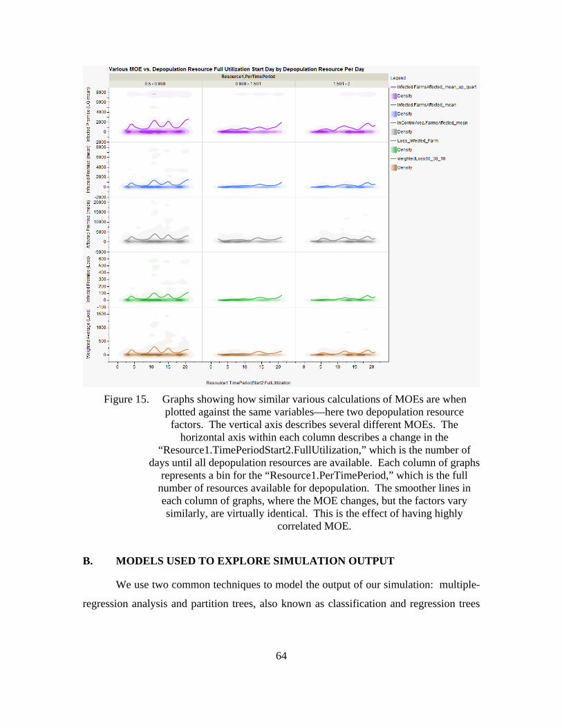
64
Figure 15. Graphs showing how similar various calculations of MOEs are when plotted against the same variables—here two depopulation resource
factors. The vertical axis describes several different MOEs. The horizontal axis within each column describes a change in the
“Resource1.TimePeriodStart2.FullUtilization,” which is the number of days until all depopulation resources are available. Each column of graphs
represents a bin for the “Resource1.PerTimePeriod,” which is the full number of resources available for depopulation. The smoother lines in each column of graphs, where the MOE changes, but the factors vary similarly, are virtually identical. This is the effect of having highly
correlated MOE.
B. MODELS USED TO EXPLORE SIMULATION OUTPUT
We use two common techniques to model the output of our simulation: multiple-
regression analysis and partition trees, also known as classification and regression trees
65
(CART). Both of these will be impacted by low correlations between the factors and the
MOEs, and by the suspected nonlinearity within the simulation. Below are descriptions
of the two techniques.
1. Multiple Regression Analysis
Multiple regression analysis seeks to explore the relationship between several
factors, called regressors, and a response variable, which we call an MOE (Montgomery,
Peck, & Vining, 2006). It does this by attempting to approximate the behavior of the
response variable with a linear equation incorporating the regressors. By observing the
coefficients of the linear equation, we are then able to identify which factors have the
greatest impact on the response variable or MOE. We evaluate the models using the
adjusted R2, a common measure to compare how models are able to describe the data.
This statistic is a score between 0 and 1 that measures how much variability is explained
by the factors in the model, but penalizes for adding insignificant factors to the model
(Montgomery, Peck, & Vining, 2006). In order for the regression to be adequate, four
assumptions about the residual errors between the actual response and the predicted
response must be met. They are: the mean of the errors must equal zero, the errors must
have constant variance, all errors are independent, and all errors are normally distributed.
The most difficult of the assumptions for us to meet is the normality assumption because
tests for normality are highly influenced by outliers, which are prevalent within our
simulations. We will test all of these assumptions for the models presented later in this
section.
2. Partition Trees
Partition trees are graphical representations of a hierarchy of questions asked of
the data to determine how they should be classified or grouped (Montgomery, Peck, &
Vining, 2006). The questions are displayed as an upside down tree, with the root at the
top containing the entire dataset. The data are then split sequentially in order to
maximize the difference in the mean of continuous factors or the probability of
categorical factors so that the nodes, or leaves, are as much alike as possible. Many
66
algorithms exist to accomplish these splits. JMP uses a log Worth calculation for
categorical factors and a Sum of Squares (SS) calculation for continuous factors (SAS,
2010).
C. IMPACT OF STARTING SCENARIOS
Since ISP is a spatial model, we expect that it will behave differently given
different starting scenarios, and that some scenarios are more likely to produce long
detection times or large outbreaks. We tested these assumptions by conducting
Tukey-Kramer HSD (honestly significant difference) comparison of means tests
(Mendenhall & Sincich, 1984) on the Detection Time mean and the Infected Premises
mean. This test calculates a single statistically significant critical difference (the HSD),
in our case at a 95% confidence level, for the mean pairs and then groups the factor
means in bins according to the computed critical difference. The results show that there
are significant differences in the behavior of the model, based on a starting scenario using
both MOEs. The Southeast Border scenario has a statistically significant lower mean
detection time, while the High Animal Density scenario has a statistically significant
higher mean number of infected premises. These results are shown in Figures 16 and 17.
Additionally, all multiple-regression models and partition trees explained in Sections D,
E, and F are first run with the starting scenario allowed in the model. In all cases, it is the
most significant factor in the model. We present the rest of our models without the
contribution of the starting scenarios, however, in order to focus on which factors
contribute most to the MOEs across all starting scenarios.
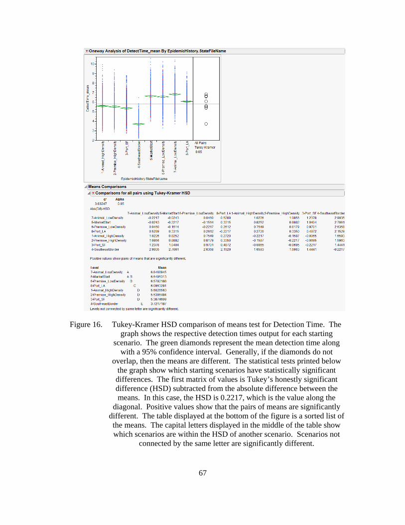
67
Figure 16. Tukey-Kramer HSD comparison of means test for Detection Time. The graph shows the respective detection times output for each starting
scenario. The green diamonds represent the mean detection time along with a 95% confidence interval. Generally, if the diamonds do not
overlap, then the means are different. The statistical tests printed below the graph show which starting scenarios have statistically significant differences. The first matrix of values is Tukey’s honestly significant difference (HSD) subtracted from the absolute difference between the means. In this case, the HSD is 0.2217, which is the value along the
diagonal. Positive values show that the pairs of means are significantly different. The table displayed at the bottom of the figure is a sorted list of the means. The capital letters displayed in the middle of the table show which scenarios are within the HSD of another scenario. Scenarios not
connected by the same letter are significantly different.

68
Figure 17. Tukey-Kramer honestly significant difference (HSD) comparison of means test for Infected Premises. The graph shows the respective number
of infected premises output for each starting scenario.
D. TIME UNTIL THE FIRST DETECTION OF AN INFECTED PREMISES
There is some debate within the literature about the importance of the length of
time between when the first premises are infected and when the first premises are
detected. Carpenter et al. (2011) use simulation to vary the length of time between when
a facility is infected and when it is detected to estimate the economic impact of the
outbreak to the United States and California, specifically. The authors find that the
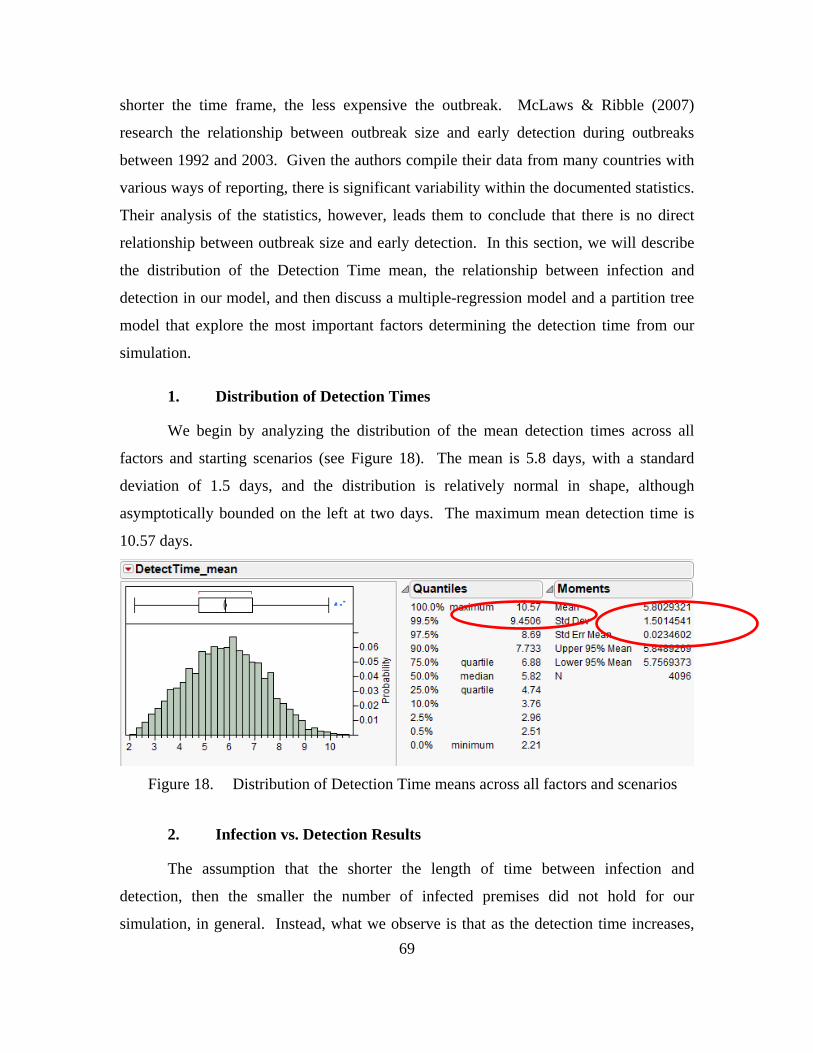
69
shorter the time frame, the less expensive the outbreak. McLaws & Ribble (2007)
research the relationship between outbreak size and early detection during outbreaks
between 1992 and 2003. Given the authors compile their data from many countries with
various ways of reporting, there is significant variability within the documented statistics.
Their analysis of the statistics, however, leads them to conclude that there is no direct
relationship between outbreak size and early detection. In this section, we will describe
the distribution of the Detection Time mean, the relationship between infection and
detection in our model, and then discuss a multiple-regression model and a partition tree
model that explore the most important factors determining the detection time from our
simulation.
1. Distribution of Detection Times
We begin by analyzing the distribution of the mean detection times across all
factors and starting scenarios (see Figure 18). The mean is 5.8 days, with a standard
deviation of 1.5 days, and the distribution is relatively normal in shape, although
asymptotically bounded on the left at two days. The maximum mean detection time is
10.57 days.
Figure 18. Distribution of Detection Time means across all factors and scenarios
2. Infection vs. Detection Results
The assumption that the shorter the length of time between infection and
detection, then the smaller the number of infected premises did not hold for our
simulation, in general. Instead, what we observe is that as the detection time increases,
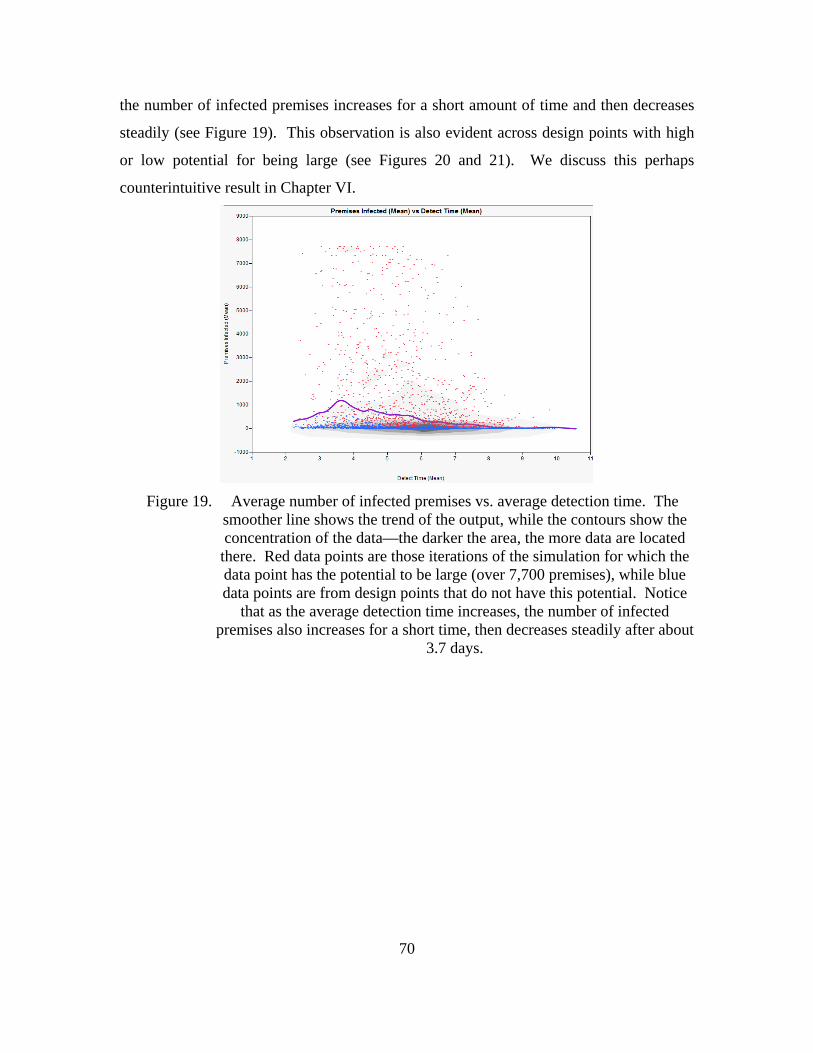
70
the number of infected premises increases for a short amount of time and then decreases
steadily (see Figure 19). This observation is also evident across design points with high
or low potential for being large (see Figures 20 and 21). We discuss this perhaps
counterintuitive result in Chapter VI.
Figure 19. Average number of infected premises vs. average detection time. The smoother line shows the trend of the output, while the contours show the concentration of the data—the darker the area, the more data are located
there. Red data points are those iterations of the simulation for which the data point has the potential to be large (over 7,700 premises), while blue data points are from design points that do not have this potential. Notice
that as the average detection time increases, the number of infected premises also increases for a short time, then decreases steadily after about
3.7 days.

71
Figure 20. Average number of infected premises vs. average detection time for scenarios (design points) with the potential of a large outbreak. Notice the
similar behavior in this figure and Figure 21.
Figure 21. Average number of infected premises vs. average detection time for scenarios with low potential of a large outbreak.
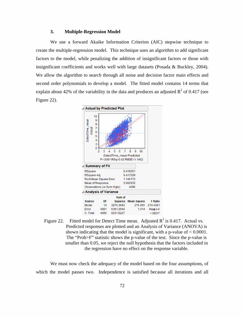
72
3. Multiple-Regression Model
We use a forward Akaike Information Criterion (AIC) stepwise technique to
create the multiple-regression model. This technique uses an algorithm to add significant
factors to the model, while penalizing the addition of insignificant factors or those with
insignificant coefficients and works well with large datasets (Posada & Buckley, 2004).
We allow the algorithm to search through all noise and decision factor main effects and
second order polynomials to develop a model. The fitted model contains 14 terms that
explain about 42% of the variability in the data and produces an adjusted R2 of 0.417 (see
Figure 22).
Figure 22. Fitted model for Detect Time mean. Adjusted R2 is 0.417. Actual vs. Predicted responses are plotted and an Analysis of Variance (ANOVA) is shown indicating that the model is significant, with a p-value of < 0.0001. The “Prob>F” statistic shows the p-value of the test. Since the p-value is smaller than 0.05, we reject the null hypothesis that the factors included in
the regression have no effect on the response variable.
We must now check the adequacy of the model based on the four assumptions, of
which the model passes two. Independence is satisfied because all iterations and all

73
design points were randomly chosen, and the residual mean is zero, as shown in
Figure 23. However, the residuals do not display constant variance (see Figure 23), nor
are they normally distributed (see Figure 24).
Figure 23. Residual by Predicted plot of multiple-regression model of the Detect Time mean. The mean of the residuals is 0, identified by the blue dashed
line; however, the residuals display heteroscedasticity.
Figure 24. Distribution of the residual errors of the multiple-regression model of the Detect Time mean. We fit the distribution to a normal curve in the right
column of the figure. Using the mean and standard deviation of the residuals, shown in the “Moments” column, JMP builds a fitted normal distribution. We then perform a Kolmogorov-Smirnov-Lillefors (KSL) Test for goodness of fit between the distribution of the residuals and the fitted normal distribution. The “Prob>D” statistic shows the p-value of
the test. Since the p-value is smaller than 0.05, we reject the null hypothesis that the distribution of residuals is normal.

74
We attempt to correct the heteroscedasticity of the residuals by performing a
transformation on the Detect Time and rerunning the forward AIC stepwise algorithm.
We select a transformation to correct the nonconstant variance and nonnormality by
trying several usual transformations including the log, square root, and exponential
(Montgomery, Peck, & Vining, 2006). Ultimately, we choose the square root
transformation because it best corrects the problems. The resulting fitted model has a
lower adjusted R2 of 0.402 (see Figure 25), but now passes the constant variance
assumption (see Figure 26). However, we were unable to meet the assumption of the
residuals being normally distributed (see Figure 27).
Figure 25. Fitted model for Square Root of Detect Time mean. Adjusted R2 is 0.402. Actual vs. Predicted responses are plotted and an Analysis of Variance
(ANOVA) is shown indicating that the model is significant, with a p-value of < 0.0001.

75
Figure 26. Residual by Predicted plot of the multiple-regression model of the Square Root of Detect Time mean. The mean of the residuals is 0, identified by
the blue dashed line, and we have removed the heteroscedasticity.
Figure 27. Distribution of the residual errors of the multiple-regression model of the Square Root of Detect Time mean. We fit the distribution to a normal
curve and perform a KSL Test for goodness of fit, which the distribution fails.
Even though our model violates the normality of residuals assumption, we present
it regardless. The factors within the model sorted by significance are presented in
Figure 28. Dairy surveillance parameters, especially the amount of delay between when
a certain premises is inspected and when it is determined to be infected
(DelayToDetection), are the most significant factors. These three parameters all have
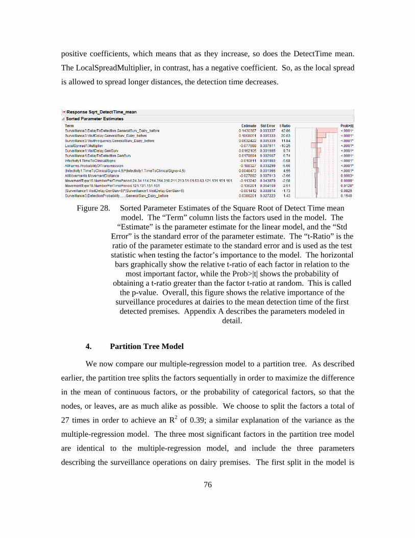
76
positive coefficients, which means that as they increase, so does the DetectTime mean.
The LocalSpreadMultiplier, in contrast, has a negative coefficient. So, as the local spread
is allowed to spread longer distances, the detection time decreases.
Figure 28. Sorted Parameter Estimates of the Square Root of Detect Time mean model. The “Term” column lists the factors used in the model. The
“Estimate” is the parameter estimate for the linear model, and the “Std Error” is the standard error of the parameter estimate. The “t-Ratio” is the ratio of the parameter estimate to the standard error and is used as the test statistic when testing the factor’s importance to the model. The horizontal bars graphically show the relative t-ratio of each factor in relation to the
most important factor, while the Prob>|t| shows the probability of obtaining a t-ratio greater than the factor t-ratio at random. This is called
the p-value. Overall, this figure shows the relative importance of the surveillance procedures at dairies to the mean detection time of the first
detected premises. Appendix A describes the parameters modeled in detail.
4. Partition Tree Model
We now compare our multiple-regression model to a partition tree. As described
earlier, the partition tree splits the factors sequentially in order to maximize the difference
in the mean of continuous factors, or the probability of categorical factors, so that the
nodes, or leaves, are as much alike as possible. We choose to split the factors a total of
27 times in order to achieve an R2 of 0.39; a similar explanation of the variance as the
multiple-regression model. The three most significant factors in the partition tree model
are identical to the multiple-regression model, and include the three parameters
describing the surveillance operations on dairy premises. The first split in the model is

77
on the amount of delay between when premises are inspected and when they are
determined to be infected (DelayToDetection). The optimal split point is at 3.411. This
means that the average Detect Time of those design points tested in the model, which
have DelayToDetection parameter settings of less than 3.411 days, are most different
from those with settings above 3.411 days. In this case, the mean Detect Time of those
design points with the DelayToDetection setting below 3.411 is 5.23 days, and the mean
of those design points above 3.411 is 6.67 days. We display the contributions of the
significant parameters in Figure 29.
Figure 29. Partition Tree model for Detect Time mean. The “Term” column shows the most significant factors affecting the mean detection time. Here, those factors are the surveillance operations on dairy premises. The “Number of
Splits” column shows how many times the partition tree was split on a factor. The “SS” column shows the sum, over the multiple splits, of the
squared differences between the two leaves into which the factor was split. Larger numbers show a larger distance between the means of the leaves.
The horizontal bars simply show the relative contribution of the factors in terms of the first factor displayed. For example, 525.2224 is
approximately 20% of 2626.9895. Therefore, the second bar is approximately 20% of the size of the first bar.
E. MEAN NUMBER OF INFECTED PREMISES
As discussed in Section A, the correlations between the MOEs we use are high.
So, here we show the models developed for the mean number of infected premises as a
proxy for the other MOE. We first describe a multiple-regression model, followed by a
partition tree.
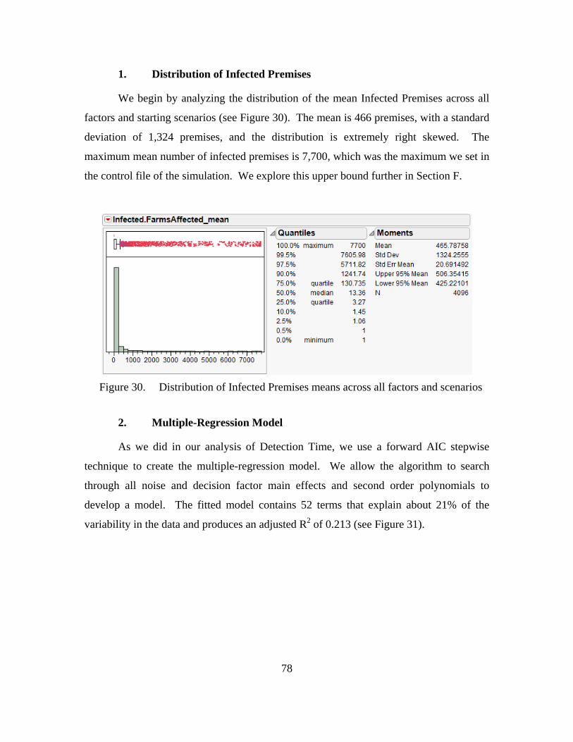
78
1. Distribution of Infected Premises
We begin by analyzing the distribution of the mean Infected Premises across all
factors and starting scenarios (see Figure 30). The mean is 466 premises, with a standard
deviation of 1,324 premises, and the distribution is extremely right skewed. The
maximum mean number of infected premises is 7,700, which was the maximum we set in
the control file of the simulation. We explore this upper bound further in Section F.
Figure 30. Distribution of Infected Premises means across all factors and scenarios
2. Multiple-Regression Model
As we did in our analysis of Detection Time, we use a forward AIC stepwise
technique to create the multiple-regression model. We allow the algorithm to search
through all noise and decision factor main effects and second order polynomials to
develop a model. The fitted model contains 52 terms that explain about 21% of the
variability in the data and produces an adjusted R2 of 0.213 (see Figure 31).

79
Figure 31. Fitted model for Infected Premises mean. Adjusted R2 is 0.213. Actual vs. Predicted responses are plotted and an Analysis of Variance (ANOVA)
is shown, indicating that the model is significant, with a p-value of < 0.0001.
We now check the adequacy of the model based on the four assumptions, of
which the model passes two. Independence is satisfied because all iterations and all
design points were randomly chosen, and the residual mean is zero, as shown in
Figure 32. However, the residuals do not display constant variance (see Figure 32), nor
are they normally distributed (see Figure 33).

80
Figure 32. Residual by Predicted plot of a multiple -egression model of the mean number of Infected Premises. The mean of the residuals is 0, identified by
the blue dashed line. We have removed the heteroscedasticity.
Figure 33. Distribution of the residual errors of the multiple-regression model of the mean number of Infected Premises. We fit the distribution to a normal
curve and perform a KSL Test for goodness of fit, which the distribution fails.
In order to address the constant variance and normality assumptions, we again
attempt to transform the response variable with one of several methods described in
Section D.3. The usual transformations do not correct the problems, however, so we
apply a Box-Cox transformation of the Infected Premises mean. Box and Cox (1964) use
a method of maximum likelihood to estimate a power to be applied to the response
variable in order to correct these problems. The resulting model contains 35 terms and

81
has an adjusted R2 of 0.323 (see Figure 34). The transformation corrects the
heteroscedasticity (see Figure 35) and the residuals appear normal, even though they fail
the goodness of fit test (see Figure 36).
Figure 34. Fitted model for Box-Cox transformed Infected Premises mean. Adjusted R2 is 0.323. Actual vs. Predicted responses are plotted and an Analysis of Variance (ANOVA) is shown indicating that the model is significant with
a p-value of < 0.0001.
Figure 35. Residual by Predicted plot of multiple regression model of the Box-Cox transformed mean number of Infected Premises. The mean of the
residuals is 0, identified by the blue dashed line. We have removed the heteroscedasticity.
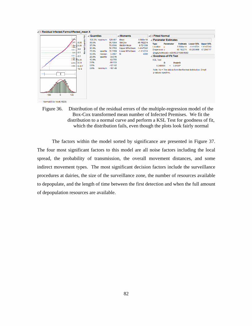
82
Figure 36. Distribution of the residual errors of the multiple-regression model of the Box-Cox transformed mean number of Infected Premises. We fit the
distribution to a normal curve and perform a KSL Test for goodness of fit, which the distribution fails, even though the plots look fairly normal
The factors within the model sorted by significance are presented in Figure 37.
The four most significant factors to this model are all noise factors including the local
spread, the probability of transmission, the overall movement distances, and some
indirect movement types. The most significant decision factors include the surveillance
procedures at dairies, the size of the surveillance zone, the number of resources available
to depopulate, and the length of time between the first detection and when the full amount
of depopulation resources are available.

83
Figure 37. Sorted Parameter Estimates of the Box-Cox transformed mean number of Infected Premises model. This shows that noise factors including the local
spread, the probability of transmission, the overall movement distances, and some indirect movement types, are the most significant factors to the mean number of infected premises. The most significant decision factors include the surveillance procedures at dairies, the size of the surveillance zone, the number of resources available to depopulate, and the length of
time between the first detection and when the full amount of depopulation resources are available. Appendix A describes the parameters modeled in
detail.
3. Partition Tree Model
We again compare our multiple-regression model to a partition tree. We choose
to split the factors a total of 50 times in order to achieve an R2 of 0.31; a similar
explanation of the variance as the multiple-regression model (see Figure 38). The noise
factors are still prevalent within the model, with the Local Spread Multiplier as the first
split. It splits at 1.5788, which is equivalent to stating that the distance bands for this
parameter are increased from the base case of 1,000 m, 2,000 m, and 3,000 m to 1,578 m,
3,157 m, and 4,736 m, respectively. Interestingly, the parameter describing the total
capacity to depopulate animals is the second split. It splits for those observations with a
Local Spread Multiplier of greater than 1.5788 at 0.638. This is equivalent to having
resources to depopulate 12,760 animals per day. The detection probability for sheep in
the surveillance zone is a factor that is not significant in any of the models up to this
point, but is in this model.

84
Figure 38. Partition Tree model for Infected Premises mean. The most significant noise factors affecting the mean number of infected premises are the Local
Spread Multiplier, the premises probability of transmission, and the detection probability of infected sheep in the surveillance zone. The most
significant decision factors are the number of resources available to depopulate, the amount of ramp-up time until all depopulation resources
are available, and the amount of delay between surveillance visits at likeDairy premises after the first infected premises of the outbreak is
detected.
F. MODELS TO EXPLORE THE POTENTIAL FOR A LARGE OUTBREAK
One concern we have with the multiple-regression and partition tree models for
the mean number of Infected Premises is that we set a maximum number of this MOE
within the simulation. Because of this, we feel that the model may be underestimating
the mean over all simulation iterations since outbreaks were stopped once the number of
infected premises reached 7,700. Therefore, we present a new MOE describing the
percentage of times a design point reached 7,700 infected premises. This MOE can be
thought of as a surrogate for whether the design point has the potential to be a large
outbreak. In this section, we describe the results obtained with the new MOE using a
multiple-regression model and with a partition tree.

85
1. Multiple-Regression Model
We add another column to our data with the frequency that the design point
reached the maximum number of infected premises out of the 100 iterations, and use this
new column as the response variable in a multiple-regression model. We exclude five
out of the seven starting scenarios because they rarely reach the maximum infected
premises limit and focus on those that do. The starting scenarios modeled using this
MOE are the High Animal Density, High Premises Density, and Port of San Francisco
scenarios. Again, we use a forward AIC stepwise technique, and allow the algorithm to
search through all noise and decision factor main effects, two-way interactions, and
second order polynomials to develop a model. The fitted model contains 45 terms, which
produces an adjusted R2 of 0.402 (see Figure 39).
Figure 39. Fitted model for Frequency Iterations with the Maximum Number of Infected Premises. Adjusted R2 is 0.402. Actual vs. Predicted responses are plotted and an Analysis of Variance (ANOVA) is shown indicating
that the model is significant, with a p-value of < 0.0001.
We again check the adequacy of the model based on the four assumptions, of
which the model passes two. Independence is satisfied because all iterations and all
design points were randomly chosen, and the residual mean is zero. However, the

86
residuals do not display constant variance, nor are they normally distributed. Again, we
attempt to transform the MOE using the usual methods, and ultimately use a log
transformation to obtain the model shown in Figure 40. The resulting model includes 45
terms and produces an adjusted R2 of 0.50. The transformed model now displays
constant variance and the residuals appear normal, even though they fail the goodness of
fit test (see Figures 41 and 42).
Figure 40. Fitted model for the Log of Frequency Iterations with the Maximum Number of Infected Premises. Adjusted R2 is 0.50. Actual vs. Predicted responses are plotted and an Analysis of Variance (ANOVA) is shown
indicating that the model is significant with a p-value of < 0.0001.
Figure 41. Residual by Predicted plot of the multiple-regression model of the log transformed Frequency of Iterations with the Maximum Number of
Infected Premises. The mean of the residuals is 0, identified by the blue dashed line. We have removed the heteroscedasticity.
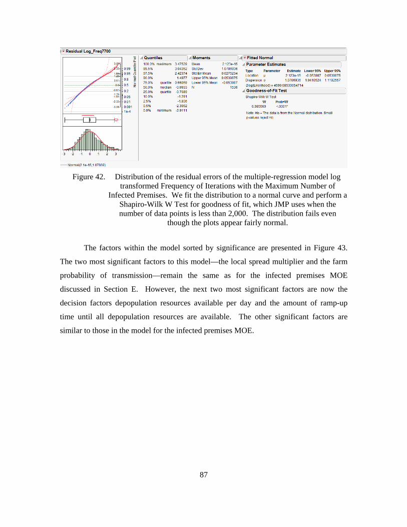
87
Figure 42. Distribution of the residual errors of the multiple-regression model log transformed Frequency of Iterations with the Maximum Number of
Infected Premises. We fit the distribution to a normal curve and perform a Shapiro-Wilk W Test for goodness of fit, which JMP uses when the number of data points is less than 2,000. The distribution fails even
though the plots appear fairly normal.
The factors within the model sorted by significance are presented in Figure 43.
The two most significant factors to this model—the local spread multiplier and the farm
probability of transmission—remain the same as for the infected premises MOE
discussed in Section E. However, the next two most significant factors are now the
decision factors depopulation resources available per day and the amount of ramp-up
time until all depopulation resources are available. The other significant factors are
similar to those in the model for the infected premises MOE.
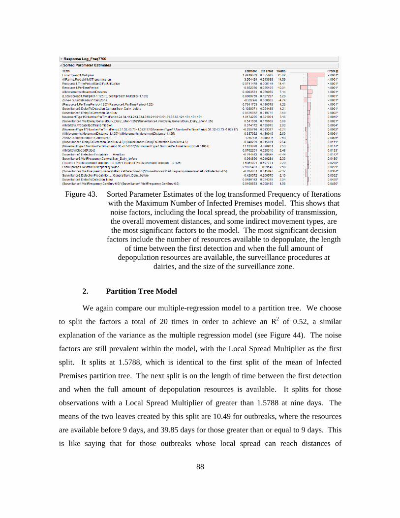
88
Figure 43. Sorted Parameter Estimates of the log transformed Frequency of Iterations with the Maximum Number of Infected Premises model. This shows that noise factors, including the local spread, the probability of transmission, the overall movement distances, and some indirect movement types, are the most significant factors to the model. The most significant decision
factors include the number of resources available to depopulate, the length of time between the first detection and when the full amount of
depopulation resources are available, the surveillance procedures at dairies, and the size of the surveillance zone.
2. Partition Tree Model
We again compare our multiple-regression model to a partition tree. We choose
to split the factors a total of 20 times in order to achieve an R2 of 0.52, a similar
explanation of the variance as the multiple regression model (see Figure 44). The noise
factors are still prevalent within the model, with the Local Spread Multiplier as the first
split. It splits at 1.5788, which is identical to the first split of the mean of Infected
Premises partition tree. The next split is on the length of time between the first detection
and when the full amount of depopulation resources is available. It splits for those
observations with a Local Spread Multiplier of greater than 1.5788 at nine days. The
means of the two leaves created by this split are 10.49 for outbreaks, where the resources
are available before 9 days, and 39.85 days for those greater than or equal to 9 days. This
is like saying that for those outbreaks whose local spread can reach distances of
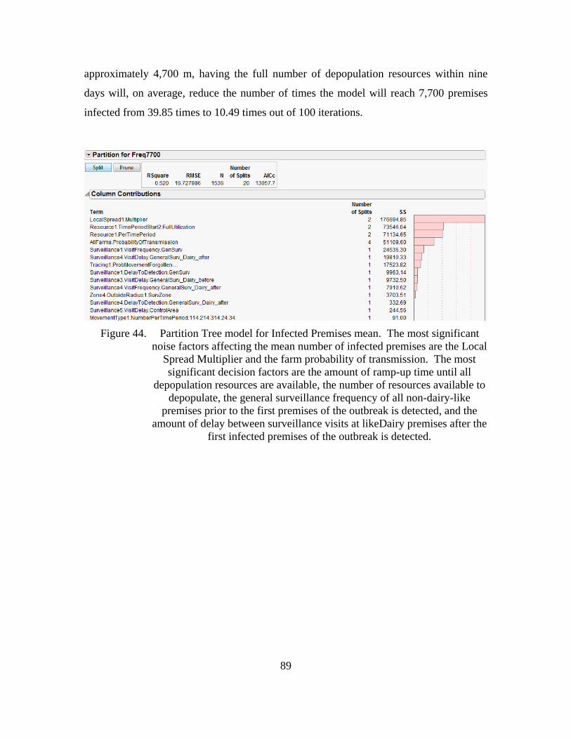
89
approximately 4,700 m, having the full number of depopulation resources within nine
days will, on average, reduce the number of times the model will reach 7,700 premises
infected from 39.85 times to 10.49 times out of 100 iterations.
Figure 44. Partition Tree model for Infected Premises mean. The most significant noise factors affecting the mean number of infected premises are the Local
Spread Multiplier and the farm probability of transmission. The most significant decision factors are the amount of ramp-up time until all
depopulation resources are available, the number of resources available to depopulate, the general surveillance frequency of all non-dairy-like
premises prior to the first premises of the outbreak is detected, and the amount of delay between surveillance visits at likeDairy premises after the
first infected premises of the outbreak is detected.

90
THIS PAGE INTENTIONALLY LEFT BLANK

91
VI. CONCLUSIONS
The results of Chapter V should not be interpreted as individual predictions on
outbreak scenarios. Instead, we vary the model 400,000 times to attempt to indicate
which parameters are the most important when modeling an outbreak in a modern,
state-of-the-art simulator, ISP. In Chapter I, we pose four research questions in order to
focus our analysis. Based on the results in Chapter V, we address those initial research
questions as well as discuss a surprising finding about depopulation resources. We
organize the sections of this chapter in the following manner:
Disease Spread Parameters: Which disease spread parameters are most
important to the simulation of an outbreak of FMD in California?
Control Area and Surveillance Zone Sizes: In response to a variety of
outbreak scenarios, what are the optimal sizes of Control Areas and
Surveillance Zones that efficiently eradicate the disease and also minimize
the economic impact to the livestock industry?
Surveillance Procedures: How often should livestock facilities be
screened for FMD prior to and during an outbreak?
Starting Scenarios: Of the outbreak scenarios modeled in this thesis,
which are the most dangerous for California?
Depopulation Resources: How do the availability and number of
depopulation resources affect the spread of FMD in California?
A. DISEASE-SPREAD PARAMETERS
Several disease parameters affect all of the models we develop. The three that
seem most significant to our models are: the Local Spread Multiplier, the All
Movements Distance Multiplier, and the Farm Probability of Transmission. Below, we
discuss these disease-spread parameters, as well as a parameter we expected to be more
significant—the movements between farms and markets.
1. The Local Spread Multiplier is a significant factor in all of the
regressions and all of the partition trees. Its effect on the mean detection time is negative,

92
meaning that as the local spread is allowed to move farther away from the infected
premises, the mean detection time decreases. This is probably because the farther the
virus moves, the more premises it comes in contact with. This leads to more premises
being infected and increases the all of the surveillance factors probabilities to detect the
disease.
The Local Spread Multiplier also has a significant effect on the size of the
outbreaks, measured both by mean number of infected premises and by the frequency of
iterations reaching 7,700 infected premises. Both MOE partition trees split first on the
Local Spread Multiplier and they split at the same point. This suggests that there may be
either an issue with the simulator at this distance of spread or that when the randomized
premises were located during the development of the data, this distance was significant in
the calculation. Whether or not this distance is truly significant is difficult to determine
since the locations of the premises are not exact. The local spread parameter serves as a
“catch all” parameter describing the spread of the disease when we are unable to
determine a reason for a premises to be infected other than its proximity to another
infected premises. So, as we begin to understand more about how the virus spreads, the
impact of the local spread parameter will likely be decreased because infections will be
able to be attributed to other causes.
2. The All Movements Distance Multiplier
The all Movements Distance Multiplier is significant in all of the regression
models, but is not significant in any of the partition trees. This parameter is similar to the
Local Spread Multiplier in that it controls how far movements of infected animals can
travel, but it is different in that movements only occur at specific rates. So, its effect on
how many other premises are infected is less direct than the local spread parameter. By
being able to move greater distances, this parameter increases the chances that the virus
will spread to a geographic area outside of the effect of local spread, or beyond the effect
of implemented control measures. This increases the probability that certain premises are
infected even though they at a lower risk from local spread or in locations outside of

93
restricted areas. The other significant characteristic of this parameter is that its effect is
greatly diminished once the first detection of infected premises is made and movement
restrictions are put in place.
3. The Farm Probability of Transmission
The Farm Probability of Transmission is significant in all of the models, which is
not surprising. The higher the probability of transmission is, the larger the outbreak is,
and the shorter the detection time is—since there is more disease to find. The fact that
this parameter shows up in all of our models is more of a confirmation that the simulation
is running correctly than an insight into the disease spread.
4. Market Movement Type 12
Market Movement Type 12 was not a factor in any of our models. This was
likely because the experimental design did not sufficiently vary the market movement
parameters and thus it is difficult to draw conclusions on their effects on the MOE.
However, the preliminary results of the plausibility models described in Chapter III are
consistent with the literature in showing that market movements are a significant
contributor to FMD spread.
B. CONTROL AREA AND SURVEILLANCE ZONE SIZES
The sizes of the control area and the surveillance zone were not as significant to
our models as we expected at the beginning of our research. The size of the surveillance
zone was always more significant than the size of the control area in our models. This is
counterintuitive since movement restrictions are tighter and surveillance for the disease is
conducted more frequently in the control areas than in the surveillance zones. It may be
that since the disease parameters so dominated our models that the effects of these zone
sizes seemed insignificant by comparison. Perhaps once we have a better understanding
of the limits of the disease parameters, the sizes of these zones will have more impact on
the models.
94
C. SURVEILLANCE
Of the 35 surveillance factors we model, two types of surveillance seem to have
the greatest significance in our models. First, all forms of likeDairy surveillance
consistently showed up as significant in our models. This is probably because
surveillance is done so frequently on these types of premises that if the virus does infect
one of them, it is detected quickly and therefore controls can be instituted quickly.
Second, the delay until detection parameters—especially on likeDairy premises, but also
generally and on traced premises—was significant to all of the regression models and
most of the partition trees. This would indicate that one way to have an effect on limiting
the size of the outbreak would be to prioritize dairy premises during lab testing so that the
amount of time between initial testing and confirmation of the virus is kept to
a minimum.
D. STARTING SCENARIOS
The most dangerous starting scenario in our model was the high animal density
model, which is not surprising. Our model reinforces the choice made by other
researchers, which is to focus on these areas of California when modeling this disease.
However, all of the starting scenarios were able to generate large outbreaks given the
correct combinations of the other parameters. Moreover, two scenarios—the high
premises dense and the San Francisco Port—were able to consistently produce large
outbreaks. This would suggest that the areas in Northern California could also be
important to study in more detail. One could also argue that since the San Francisco Port
is able to consistently produce large outbreaks, maintenance of surveillance resources at
international ports is justified. Since we did not observe the same consistency of large
outbreaks from the Los Angeles Port scenario, however, we feel that additional
exploration of port scenarios is needed before making that claim.
E. DEPOPULATION RESOURCES
Two decision factors that were consistently significant to our models were the two
depopulation resource parameters that described how many resources were available per
day and how quickly those resources could be available. The partition trees split on these
95
parameters at about 12,000 animals per day and at a ramp-up time of less than nine days.
These factors are probably so significant because there was not a preemptive culling
strategy implemented in our model and because the local spread probabilities were not
reduced based on detection of the disease on a premises. So, in order to control the
disease, depopulation resources had to be readily available in large supply to quickly
depopulate premises that became infected. If perfect biosecurity was established at the
time of quarantine, and aerosol transmission was not a significant factor, then the disease
should not spread from the premises. Therefore, our conclusions about the depopulation
resources are also linked to the fact that we did not model the effect of biosecurity on the
local spread parameters. Sensitivity analysis should be conducted to determine how these
two parameters interact.
F. SUMMARY
Even though our models had relatively low adjusted R2 values, we believe they
still give us a fair amount of insight into the characteristics of the spread and control of an
FMD outbreak in California. We believe that there are two major takeaways from our
research for policymakers, and some for FMD researchers. We present the former below,
and the latter in Chapter VII.
The most important disease surveillance is done at likeDairy premises.
We see the surveillance parameters of likeDairy premises as significant to
both the detection time and size of outbreak regression models and
partition trees. This is likely because these types of premises usually have
personnel on staff who have daily contact with their animals and that the
clinical signs of infection in cattle are generally easier to detect than in
other species. These characteristics lead to decreased time until detection,
which leads to quicker implementation of controls and smaller outbreaks.
Continued research into how to make this type of surveillance as efficient
as possible could have a significant impact on how large an outbreak
becomes if it ever occurs in California.

96
The size and availability of depopulation resources are significant in all of
the size of outbreak models. Unlike many other authors’ models and due
to our understanding of the current views in California, we do not use
preemptive depopulation in our model. Since we only depopulate detected
premises and do not explore the effects of biosecurity on the local spread
from those premises, we must accomplish depopulation as efficiently as
possible to prevent or limit the spread of the disease. This requires the
availability of large amounts of resources in a timely matter. Our model
suggests the amount of resources necessary could be the ability to
depopulate over 12,000 animals per day within nine days of the first
detection of infected livestock premises. If the state does not plan on
using preemptive depopulation, then this magnitude of depopulation
resources should be readily available on a very short ramp-up timeline to
facilitate the rapid control of an FMD outbreak.
97
VII. RECOMMENDATIONS FOR FUTURE RESEARCH
We feel that there are several areas where our research could be improved. When
discussing the benefits of a simulation experimental design, Sanchez (2008, p. 83) writes,
“This process typically follows an iterative cycle, where insights gained from
simulation experiments can be used in many ways. Results can be used to
evaluate or improve the simulation model. By identifying important factors,
interactions, and nonlinear effects, the experimenter can improve their
understanding, find robust solutions, or raise questions to be explored in
subsequent experiments. Thresholds, plateaus, or other interesting features of the
response surfaces might provide guidance about situations that are particularly
good (or particularly bad).”
This thesis is one step in the iterative cycle of which Sanchez writes. During the
rest of this chapter, we will discuss the changes that are needed or which would be
interesting to explore in the ISP control file, the experimental design, the output statistics,
and more general areas we feel should be further researched regarding the spread of FMD
in California.
A. ISP CONTROL FILE
The development of the ISP control file was a difficult task due to the complexity
and sheer number of parameters included in our simulation. Below is a list of the
changes or fixes we recommend to those who would conduct follow-on research using
ISP to model an outbreak of FMD in California.
Parameterize Dairy Tanker movement as “Fixed Routes”: Our results
indicate that the diary premises in California have a significant impact on
FMD control, and those premises also make up a large part of California’s
agricultural economic output. Our model could be improved by
specifically modeling the movements of vehicles on and off of dairy
premises. Data on tanker movements would be extremely useful, whether
98
gathered from industry groups, where the data resides, or from
government organizations interested in controlling FMD.
Parameterize Airborne Spread: Airborne spread can be an important
factor for some FMD serotypes (Stevenson, 2012). Future models could
benefit from adding predominant winds within the state. This may be
especially important for areas of the state that are not within a “local
spread” distance from a large farm, which can produce significant virus
plumes, but may be downwind of one that is farther away.
Surveillance Zone Parameters: In our base control file, we did not
correctly use the option to preempt a premises being added to the
surveillance zone if it had already been added to a control area. This did
not affect our results since we corrected for this oversight in the output
data. Future researchers should set the parameter “ExcludeFarmsInZones”
to the zone name for the control area.
County Zones: Radial zones are difficult to manage during an outbreak
and would not generally be used under USDA guidelines (USDA, 2011).
More likely, counties or similar-sized areas would be designated as certain
zones or areas. ISP does not currently have the functionality to apply
zones in this manner, but there may be ways to accomplish this in future
updates to the software.
Restricting Movements on Farm Class: Our model restricts all
movements within a zone equally after the first detection of infected
premises. This is perhaps not the best strategy given that some premises
are more infectious, or have other applicable characteristics, than others.
If strategies can be found that reduce the impact of movement restrictions
on some premises, the overall impact on the California livestock industry
could be reduced. The first step would be to quantify how much

99
movement restrictions actually hurt a livestock premises and then attempt
to minimize the overall economic impact on the state, as opposed to
surrogates such as the number of premises affected or infected.
Probabilities of Contact Between Farm Types: Our model does not use
the “RestrictOnAnimalType” or “RestrictOnFarmClass” parameters for
direct and indirect movements. These parameters allow the user to specify
restrictions to the destinations of specific movements. An example of this
type of restriction is for direct contact movements originating from small
swine premises to only be allowed to have destinations at other swine
premises. Or, more specifically, for those same movements to only be
allowed to have destinations at other small swine premises. We did not
use them due to the complexity they add, as well as the fact that only one
animal type is present on each of the premises in our data. However,
adding these parameters would more closely resemble actual contact
between premises.
Regional Movement Standstill: Pineda-Krch et al. (2010) found that
setting up a statewide movement ban on all livestock movements was
beneficial in their research. While we believe that a statewide ban may
not be necessary, given the large distances between livestock production
regions within the state, we feel that future research should compare the
impact of statewide “movement standstills” to more regionalized
movement restrictions such as overlapping northern, central, and southern
regions. ISP does have parameters to allow for such a comparison.
Regional California Dataset: Due to the number of and geographic
distances between the premises in our dataset, the development of smaller
regional models, or a small mock “California,” would allow closer
examination of each factor. This may also help to more easily evaluate
model behavior and identify problems with parameterization or bugs in the
implementation of the software.
100
B. DESIGN OF THE EXPERIMENT (DOE)
The most difficult part of designing the experiment was in setting the high and
low limits of each parameter studied. Based on the results of our model, we suggest the
following modifications to the DOE:
Surveillance Rates: The surveillance rates’ high and low limits were
generally set fairly wide apart in order to estimate their overall effect
within the model. Now that we understand their importance to the model,
more thought and expertise should be applied towards finding more
realistic rates for each surveillance type. This could then give more
fidelity to where limited surveillance resources should be applied.
Farm Probability of Transmission: Our DOE currently applies low and
high limits on farm probability of transmission from sheep and goats to
0% and 50%, respectively. We then apply a function to that probability in
order to determine the probabilities for cattle and swine farms. After
further review, this function for cattle may not allow probabilities to be as
high as they should be when modeling direct and indirect contact between
animals. We believe the exponent used should be closer to 15 instead of
1.82, in order to better model how much virus is shed by cattle by means
other than aerosol, which is how we determine the current exponent used
in the function.
Rate of Market Movement: McLaws and Ribble (2007) propose that the
factor that contributes most to an FMD outbreak becoming a large is virus
movement through markets. However, we do not vary the number of
farm-to-market movements per time period in our current design due to
insufficient understanding of this parameter in the literature. Future
research should vary this rate based on subject matter expert
understanding or funding should be made available to collect data in order
to better understand the spread of the virus prior to the first detection of
infected premises.
101
Local Spread Multiplier Limits: As discussed in Chapter VI, local
spread is a dominant factor within our model. Since the first splits within
all the partition trees we use in our analysis are on a local spread multiplier
of approximately 1.6, which equates to a maximum distance band of
roughly 4,800 m, it may merit checking the ISP software for
idiosyncrasies at around the 5,000 m value. If such an anomaly exists
within the software, our model may have more reliable results if the
maximum local spread distance can be kept under that size.
Greater SME Input and Review: The DOE high and low limits were set
to widely vary the parameter settings as a first step in observing the effects
of those factors. Now that we understand a bit more about these effects,
SMEs should be used to narrow these ranges and therefore obtain more
realistic outbreak results.
C. ADDITIONAL OUTPUT
In order to organize the simulation output for analysis, we use several scripts to
read the output files developed by ISP during the simulation and calculate the MOEs we
use for our analysis. Knowing the results of our analysis, we believe that three additional
measures should be calculated by this script in order to further our understanding of the
outbreaks simulated.
Day of last infection and/or day of last detection during each
simulation iteration: Currently, our model does not have a way to
measure if or when the outbreak ended during the course of the
simulation. For example, setting a time period of a certain number of
days, say 28 days, since a detection would declare the epidemic over.
Having this information would allow us to better understand the
effectiveness of the control strategies.
The number of infected premises when the first detection occurs
during each iteration: We believe that we would better understand the
relationship between the outbreak size and detection time if we knew how

102
fast the silent spread, the disease spread prior to first detection, is moving.
Our belief is that when the outbreak spreads quickly, the virus is easier to
detect. This is because we sample the susceptible population at a certain
rate, and when more premises are infected, the time it takes to find an
infected facility decreases. Having the number of infected premises and
the types of those premises at the first detection would allow us to more
fully explore this belief.
The locations of the randomly selected initially infected premises:
These locations should have been preserved in order to conduct some
additional location-based analysis. We believe our starting scenarios do a
good job of capturing the outbreak characteristics based on densities of
animals or premises, but may not fully capture the geographic
characteristics of California. Having more information about the exact
initially infected premises location may better inform this area.
The projected number of infected premises when an iteration reaches
the maximum number of infected premises: Since our iterations were
cut off when the number of infected premises reached 7,700, we had to
develop a surrogate MOE to study the largest outbreaks. If the number of
infected premises could be accurately projected, a surrogate MOE would
not have to be used.
D. GENERAL RESEARCH
This thesis makes several assumptions because of either our lack of understanding
or by an absence in the literature of several areas impacting a potential outbreak of FMD
or any foreign animal disease in California. In this section, we describe two areas we feel
need additional emphasis, research, or published information by the scientific community
to inform the modeling of livestock diseases in the state.
Better knowledge of facility locations/species mix: Because the data we
used to construct our model were developed from publicly available,
county-level aggregated statistics of livestock premises, they only
103
approximate the locations, sizes, animal types, and production types of the
livestock premises in the state. Since ISP uses all of these characteristics
to determine how the virus spreads, if the actual characteristics differ
greatly from the approximate characteristics, the virus spread could also
vary greatly.
E. KNOWLEDGE OF DIRECT AND INDIRECT MOVEMENT RATES AT LOCATIONS OUTSIDE OF CENTRAL CALIFORNIA:
Since the direct and indirect movement distances and probabilities were generated
from a study of only central California, we may be over or underestimating the outbreaks
in other areas of the state. Having better knowledge of these movements in other areas
could help in better defining high-risk locations/regions of the state.
F. FINAL REMARKS
FMD is a fast-moving disease with potentially catastrophic consequences for
California and the United States. It is important that policy makers are prepared to
respond effectively and immediately if and when an outbreak occurs. Circumstances and
details of an outbreak can greatly affect the behavior and consequences. There will not
be time for model development during a crisis, so timely analysis requires having the
appropriate models in reserve. This thesis takes an important step toward this ultimate
objective.

104
THIS PAGE INTENTIONALLY LEFT BLANK
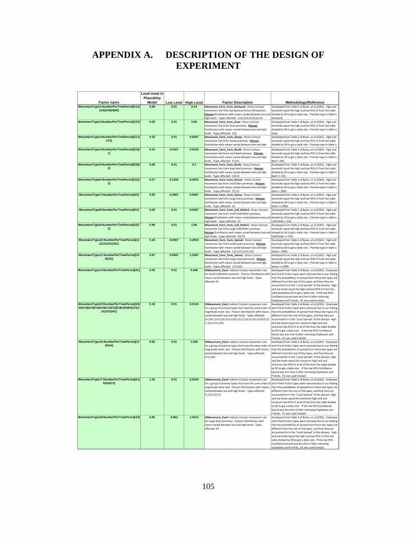
105
APPENDIX A. DESCRIPTION OF THE DESIGN OF EXPERIMENT
Factor name
Level Used in Plausiblity
Model Low Level High Level Factor Description Methodology/ReferenceMovementType1:NumberPerTimePeriod[114|
214|314|24|34]0.08 0.01 0.14 Movement_Farm_Farm_Backyard: Direct Contact
movement rate from backyard premises (All Species).
Poisson Distribution with means varied between low and
high levels. Types affected: 114|214|314|24|34
Developed from Table 2 of Bates, et al (2001). High and
low levels equal the high and low 95% CI from the table
divided by 30 to get a daily rate. Premise type in table is
Backyard.
MovementType2:NumberPerTimePeriod[310] 0.29 0.01 0.56 Movement_Farm_Farm_Goat: Direct Contact
movement rate from Goat premises. Poisson
Distribution with means varied between low and high
levels. Types affected: 310
Developed from Table 2 of Bates, et al (2001). High and
low levels equal the high and low 95% CI from the table
divided by 30 to get a daily rate. Premise type in table is
Goat.
MovementType3:NumberPerTimePeriod[211|213]
0.32 0.01 0.6267 Movement_Farm_Farm_Sheep: Direct Contact
movement rate from Sheep premises. Poisson
Distribution with means varied between low and high
l l T ff d 211|213
Developed from Table 2 of Bates, et al (2001). High and
low levels equal the high and low 95% CI from the table
divided by 30 to get a daily rate. Premise type in table is
ShMovementType4:NumberPerTimePeriod[51|61]
0.03 0.0167 0.0433 Movement_Farm_Farm_BeefS: Direct Contact
movement rate from smal Beef premises. Poisson
Distribution with means varied between low and high
levels. Types affected: 51|61
Developed from Table 2 of Bates, et al (2001). High and
low levels equal the high and low 95% CI from the table
divided by 30 to get a daily rate. Premise type in table is
Beef < 250.
MovementType5:NumberPerTimePeriod[53|63]
0.06 0.01 0.1 Movement_Farm_Farm_BeefL: Direct Contact
movement rate from large Beef premises. Poisson
Distribution with means varied between low and high
levels. Types affected: 53|63
Developed from Table 2 of Bates, et al (2001). High and
low levels equal the high and low 95% CI from the table
divided by 30 to get a daily rate. Premise type in table is
Beef >= 250.
MovementType6:NumberPerTimePeriod[31|32]
0.27 0.1433 0.4033 Movement_Farm_Farm_DairyS: Direct Contact
movement rate from Small Dairy premises. Poisson
Distribution with means varied between low and high
levels. Types affected: 31|32
Developed from Table 2 of Bates, et al (2001). High and
low levels equal the high and low 95% CI from the table
divided by 30 to get a daily rate. Premise type in table is
Dairy < 1000.
MovementType7:NumberPerTimePeriod[33] 0.55 0.3967 0.6967 Movement_Farm_Farm_DairyL: Direct Contact
movement rate from Large Dairy premises. Poisson
Distribution with means varied between low and high
levels. Types affected: 33
Developed from Table 2 of Bates, et al (2001). High and
low levels equal the high and low 95% CI from the table
divided by 30 to get a daily rate. Premise type in table is
Dairy >= 2000.
MovementType8:NumberPerTimePeriod[41] 0.02 0.01 0.0367 Movement_Farm_Farm_Calf_HeiferS: Direct Contact
movement rate from Small Calf/Heifer premises.
Poisson Distribution with means varied between low and
high levels. Types affected: 41
Developed from Table 2 of Bates, et al (2001). High and
low levels equal the high and low 95% CI from the table
divided by 30 to get a daily rate. Premise type in table is
Calf/Heifer < 250.
MovementType9:NumberPerTimePeriod[43|73]
0.99 0.01 1.96 Movement_Farm_Farm_Calf_HeiferL: Direct Contact
movement rate from Large Calf/Heifer premises.
Poisson Distribution with means varied between low and
high levels. Types affected: 43|73
Developed from Table 2 of Bates, et al (2001). High and
low levels equal the high and low 95% CI from the table
divided by 30 to get a daily rate. Premise type in table is
Calf/Heifer >= 250.
MovementType10:NumberPerTimePeriod[121|131|151|161]
0.16 0.0367 0.2833 Movement_Farm_Farm_SwineS: Direct Contact
movement rate from Small Swine premises. Poisson
Distribution with means varied between low and high
levels. Types affected: 121|131|151|161
Developed from Table 2 of Bates, et al (2001). High and
low levels equal the high and low 95% CI from the table
divided by 30 to get a daily rate. Premise type in table is
Swine < 2000.
MovementType11:NumberPerTimePeriod[153|163]
0.67 0.0067 1.3267 Movement_Farm_Farm_SwineL: Direct Contact
movement rate from Large Swind premises. Poisson
Distribution with means varied between low and high
levels. Types affected: 153|163
Developed from Table 2 of Bates, et al (2001). High and
low levels equal the high and low 95% CI from the table
divided by 30 to get a daily rate. Premise type in table is
Swine >= 2000.
MovementType14:NumberPerTimePeriod[41] 0.03 0.01 0.046 IDMovement_Size1: Indirect Contact movement rate
for Small Calf/Heifer premises. Poisson Distribution with
means varied between low and high levels. Types
affected: 41
Developed from Table 3 of Bates, et al (2001). Employee
and Friend Visitor types were removed due to our feeling
that the probabilities of spread from those two types are
different from the rest of the types, and that they are
accounted for in the "Local Spread" of the disease. High
and low levels equal the high and low 95% CI from the
table divided by 30 to get a daily rate. If the low 95%
Confidence bound was less than 0 after removing
Employees and Friends, .01 was used instead.
MovementType15:NumberPerTimePeriod[24|34|114|214|314|310|211|213|51|61|53|63|121|1
31|151|161]
0.16 0.01 0.3143 IDMovement_Size2: Indirect Contact movement rate
for a group of premise types that have the same order of
magnitude mean rate. Poisson Distribution with means
varied between low and high levels. Types affected:
24|34|114|214|314|310|211|213|51|61|53|63|12
1|131|151|161
Developed from Table 3 of Bates, et al (2001). Employee
and Friend Visitor types were removed due to our feeling
that the probabilities of spread from those two types are
different from the rest of the types, and that they are
accounted for in the "Local Spread" of the disease. High
and low levels equal the maximum high and and
minimum low 95% CI of all of the from the table divided
by 30 to get a daily rate. If the low 95% Confidence
bound was less than 0 after removing Employees and
Friends, .01 was used instead.
MovementType16:NumberPerTimePeriod[153|163]
0.82 0.01 1.626 IDMovement_Size3: Indirect Contact movement rate
for a group of premise types that have the same order of
magnitude mean rate. Poisson Distribution with means
varied between low and high levels. Types affected:
153|163
Developed from Table 3 of Bates, et al (2001). Employee
and Friend Visitor types were removed due to our feeling
that the probabilities of spread from those two types are
different from the rest of the types, and that they are
accounted for in the "Local Spread" of the disease. High
and low levels equal the maximum high and and
minimum low 95% CI of all of the from the table divided
by 30 to get a daily rate. If the low 95% Confidence
bound was less than 0 after removing Employees and
Friends, .01 was used instead.
MovementType17:NumberPerTimePeriod[31|32|43|73]
1.02 0.01 2.0343 IDMovement_Size4: Indirect Contact movement rate
for a group of premise types that have the same order of
magnitude mean rate. Poisson Distribution with means
varied between low and high levels. Types affected:
31|32|43|73
Developed from Table 3 of Bates, et al (2001). Employee
and Friend Visitor types were removed due to our feeling
that the probabilities of spread from those two types are
different from the rest of the types, and that they are
accounted for in the "Local Spread" of the disease. High
and low levels equal the maximum high and and
minimum low 95% CI of all of the from the table divided
by 30 to get a daily rate. If the low 95% Confidence
bound was less than 0 after removing Employees and
Friends, .01 was used instead.
MovementType18:NumberPerTimePeriod[33] 0.95 0.862 1.0413 IDMovement_Size5: Indirect Contact movement rate
for Large Dairy premises. Poisson Distribution with
means varied between low and high levels. Types
affected: 33
Developed from Table 3 of Bates, et al (2001). Employee
and Friend Visitor types were removed due to our feeling
that the probabilities of spread from those two types are
different from the rest of the types, and that they are
accounted for in the "Local Spread" of the disease. High
and low levels equal the high and low 95% CI from the
table divided by 30 to get a daily rate. If the low 95%
Confidence bound was less than 0 after removing
Employees and Friends, .01 was used instead.
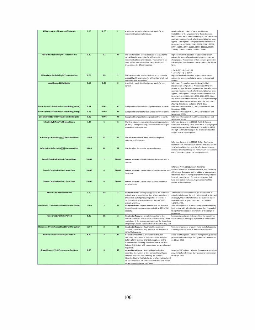
106
AllMovements:MovementDistance 1.13 0.25 2 A multiplier applied to the distance bands for all
movement types simultaneously.
Developed from Table 3 of Bates, et al (2001).
Probabilities of the virus moving to these distances
remains fixed across all movement types, but refer to the
updated movement bands after the multiplier has been
applied. A multiplier = 1 will produce movement bands
(in meters) of: 0‐19000, 19001‐39000, 39001‐59000,
59001‐79000, 79001‐99000, 99001‐119000, 119001‐
139000, 139001‐159000, 159001‐179000.
AllFarms:ProbabilityOfTransmission 0.30 0.1 0.5 The constant to be used as the basis to calculate the
probability of transmission for all farm to farm
movements (Direct and Indirect). This number is an
input to functions to calculate the probability of
transmission for different species.
High and low levels based on subject matter expert
opinion for farm to farm direct or indirect contact for
sheep/goats. This constant is then an input (p) into the
following functions based on species type on the source
farm.
> Cattle POT = 1‐(1‐p)^1.82
> Swine POT = 1‐(1‐p)^80
AllMarkets:ProbabilityOfTransmission 0.75 0.5 1 The constant to be used as the basis to calculate the
probability of transmission for all farm to market and
market to farm movements.
High and low levels based on subject matter expert
opinion for farm to market and market to farm direct
contact.
LocalSpread1:Multiplier 1.13 0.25 2 A multiplier applied to the distance bands for local
spread.
Reference: Personal communication with Mark
Stevenson on 11 Apr 2012. Probabilities of the virus
moving to these distances remains fixed, but refer to the
updated movement bands after the multiplier has been
applied. A multiplier = 1 will produce movement bands
(in meters) of: 0‐1000, 1001‐2000, 2001‐3000. Note:
The probabilities of transmission for Local Spread change
over time. Local spread initiates when the farm starts
showing clinical signs and stops after 6 days.
LocalSpread1:RelativeSusceptibility[swine] 0.01 0.001 0.1 Suceptability of swine to local spread relative to cattle. Reference (Donaldson et al., 2001; Alexanderson and
Donaldson, 2002).
LocalSpread1:RelativeSusceptibility[sheep] 0.05 0.005 0.5 Suceptability of sheep to local spread relative to cattle. Reference (Donaldson et al., 2001; Alexanderson and
Donaldson, 2002).
LocalSpread1:RelativeSusceptibility[goat] 0.05 0.005 0.5 Suceptability of goat to local spread relative to cattle. Reference (Donaldson et al., 2001; Alexanderson and
Donaldson, 2002).
Infectivity1:TimeToClinicalSigns 4.38 1 8 The Beta value of a LogLogistic Curve with parameters
(2, Beta, 4.1436) describing the time until clinical signs
are evident on the premise.
Reference Sanson, et al (2006b). Table 2 shows a
cumulative probability table, which we fit to a LogLogistic
Curve with parameters (0,beta=4.3770,alpha=4.1436)
The high and low levels adjust the B value are based on
subject matter expert opinion.
Infectivity1:Infectivity[][][]:DecreaseStart 17.00 12 22 The day after infection when infectivity begins to
decrease on the premise.
Infectivity1:Infectivity[][][]:DecreaseEnd 33.00 28 38 The day when the premise becomes immune.
Zone2:OutsideRadius1:ControlArea 10001 1 20000 Control Measure: Outside radius of the control area in
meters.
Zone3:OutsideRadius1:VaccZone 10000 0 20000 Control Measure: Outside radius of the vaccination zone
in meters.
Zone4:OutsideRadius1:SurvZone 25000 0 50000 Control Measure: Outside radius of the Surveillance
zone in meters.
Resource1:PerTimePeriod 1.00 0.5 2 DepopResource: a multiplier applied to the number of
animals able to be culled in a day. When multiplier = 1,
the animals culled per day (regardless of species) =
20,000 animals after full utilization day, and 2000
animals until then.
20000 animals developed from the total number of
animals culled during the U.K. FMD outbreak (4.5M) and
dividing by the number of months the outbreak lasted
multiplied by 30 to give a daily rate. i.e.: 20000 =
4.5M/(7.5*30).
Resource1:TimePeriodStart2:FullUtilization 11.00 2 21 DepopResource: Day that all Resources are available.
Up until this day, resources are available at 10% of full
capacity.
Tests the importance of a quick ramp up to full capacity.
Early testing with full utilization longer than 21 days led
to significant increases in the runtime of the design of
experiment.
Resource2:PerTimePeriod 1.00 0.5 2 VaccinationResource: a multiplier applied to the
number of animals able to be vaccinated in a day. When
multiplier = 1, the animals vaccinated per day (regardless
of species) = 20,000 animals after full utilization day, and
Same as depopulation. Estimated that the capacity to
vaccinate would be roughly equivalent to depopulation.
Resource2:TimePeriodStart2:FullUtilization 11.00 2 21 VaccinationResource: Day that all Resources are
available. Up until this day, resources are available at
10% of full capacity.
Tests the importance of a quick ramp up to full capacity.
Same high and low levels as depopulation resource.
Surveillance1:VisitDelay:GenSurv 6.00 2 10 GeneralSurveillance: A probability distribution
describing the number of time periods that will pass
before a farm is visited prior to being placed on the
surveillance list following a detected farm in the area.
Poisson Distribution with means varied between low and
high levels.
Based on SME opinion. Adapted from general guidelines
provided by Pam Hullinger during personal conversation
on 12 Apr 2012.
Surveillance1:VisitFrequency:GenSurv 6.50 3 10 GeneralSurveillance: A probability distribution
describing the number of time periods that will pass
between visits to a farm following the first visit
(described by the VisitDelay) prior to a farm being placed
on the surveillance list. Poisson Distribution with means
varied between low and high levels.
Based on SME opinion. Adapted from general guidelines
provided by Pam Hullinger during personal conversation
on 12 Apr 2012.
Reference Sanson, et al (2006b). Delphi Conference
estimated that premise would be most infectious on day
16 after initial infection, and the infectiousness would
decrease linearly until day 33. Here we vary the start and
end of the infectiousness decline by +/‐ 5 days.
Reference APHIS (2012), Ready Reference
Guide—Quarantine, Movement Control, and Continuity
of Business. Developed radii by adding or subtracting a
reasonable distance from published minimum guidelines
for small control areas. Once other parameter limits
have been better evaluated, larger zones should be
studied within the design.

107
Surveillance1:DelayToDetection:GenSurv 4.50 2 7 GeneralSurveillance: A probability distribution
returning the number of time periods from when the
visit occurred to when that farm will receive the
detected state (prior to a farm being placed on the
surveillance list). Poisson Distribution with means varied
between low and high levels.
Based on SME opinion. Adapted from general guidelines
provided by Pam Hullinger during personal conversation
on 12 Apr 2012.
Surveillance1:DetectionProbability[][][]:GenSurv
0.50 0 0.99 GeneralSurveillance: A function describing the
probability of an infected farm being detected at each
visit by the number of time periods since the farm was
infected. In our case, the function is constant, but
would vary between the Lo and Hi values shown.
Based on SME opinion. Adapted from general guidelines
provided by Pam Hullinger during personal conversation
on 12 Apr 2012.
Surveillance1:DetectionProbability[][][sheep]:GenSurv
0.48 0 0.95 GeneralSurveillance: A function describing the
probability of an infected Sheep farm being detected at
each visit by the number of time periods since the farm
was infected. In our case, the function is constant, but
would vary between the Lo and Hi values shown.
Based on SME opinion. Adapted from general guidelines
provided by Pam Hullinger during personal conversation
on 12 Apr 2012.
Surveillance2:VisitDelay:GeneralAfterFirstDetection
4.50 2 7 GeneralSurveillance_AfterDetect: A probability
distribution describing the number of time periods that
will pass before a farm is visited after being placed on
the surveillance list following a detected farm in the
area. Poisson Distribution with means varied between
low and high levels.
Based on SME opinion. Adapted from general guidelines
provided by Pam Hullinger during personal conversation
on 12 Apr 2012.
Surveillance2:VisitFrequency:GeneralAfterFirstDetection
4.50 2 7 GeneralSurveillance_AfterDetect: A probability
distribution describing the number of time periods that
will pass between visits to a farm following the first visit
(described by the VisitDelay) while a farm is on the
surveillance list. Poisson Distribution with means varied
between low and high levels.
Based on SME opinion. Adapted from general guidelines
provided by Pam Hullinger during personal conversation
on 12 Apr 2012.
Surveillance2:DelayToDetection:GeneralAfterFirstDetection
3.00 1 5 GeneralSurveillance_AfterDetect: A probability
distribution returning the number of time periods from
when the visit occurred to when that farm will receive
the detected state. Poisson Distribution with means
varied between low and high levels.
Based on SME opinion. Adapted from general guidelines
provided by Pam Hullinger during personal conversation
on 12 Apr 2012.
Surveillance2:DetectionProbability[][][]:GeneralAfterFirstDetection
0.90 0.8 0.99 GeneralSurveillance_AfterDetect: A function
describing the probability of an infected farm being
detected at each visit by the number of time periods
since the farm was infected. In our case, the function is
constant, but would vary between the Lo and Hi values
shown.
Based on SME opinion. Adapted from general guidelines
provided by Pam Hullinger during personal conversation
on 12 Apr 2012.
Surveillance2:DetectionProbability[][][sheep]:GeneralAfterFirstDetection
0.83 0.7 0.95 GeneralSurveillance_AfterDetect: A function
describing the probability of an infected Sheep farm
being detected at each visit by the number of time
periods since the farm was infected. In our case, the
function is constant, but would vary between the Lo and
Hi values shown.
Based on SME opinion. Adapted from general guidelines
provided by Pam Hullinger during personal conversation
on 12 Apr 2012.
Surveillance3:VisitDelay:GeneralSurv_Dairy_before
1.75 0.5 3 GeneralSurv_Dairy_before: A probability distribution
describing the number of time periods that will pass
before a farm is visited after being placed on the
surveillance list following a detected farm in the area.
Poisson Distribution with means varied between low and
high levels.
Based on SME opinion. Adapted from general guidelines
provided by Pam Hullinger during personal conversation
on 12 Apr 2012.
Surveillance3:VisitFrequency:GeneralSurv_Dairy_before
1.75 0.5 3 GeneralSurv_Dairy_before: A probability distribution
describing the number of time periods that will pass
between visits to a farm following the first visit
(described by the VisitDelay) while a farm is on the
surveillance list. Poisson Distribution with means varied
between low and high levels.
Based on SME opinion. Adapted from general guidelines
provided by Pam Hullinger during personal conversation
on 12 Apr 2012.
Surveillance3:DelayToDetection:GeneralSurv_Dairy_before
3.00 1 5 GeneralSurv_Dairy_before: A probability distribution
returning the number of time periods from when the
visit occurred to when that farm will receive the
detected state. Poisson Distribution with means varied
between low and high levels.
Based on SME opinion. Adapted from general guidelines
provided by Pam Hullinger during personal conversation
on 12 Apr 2012.
Surveillance3:DetectionProbability[][][]:GeneralSurv_Dairy_before
0.75 0.5 0.99 GeneralSurv_Dairy_before: A function describing the
probability of an infected farm being detected at each
visit by the number of time periods since the farm was
infected. In our case, the function is constant, but
would vary between the Lo and Hi values shown.
Based on SME opinion. Adapted from general guidelines
provided by Pam Hullinger during personal conversation
on 12 Apr 2012.
Surveillance4:VisitDelay:GeneralSurv_Dairy_after
1.25 0.5 2 GeneralSurv_Dairy_after: A probability distribution
describing the number of time periods that will pass
before a farm is visited after being placed on the
surveillance list following a detected farm in the area.
Poisson Distribution with means varied between low and
Based on SME opinion. Adapted from general guidelines
provided by Pam Hullinger during personal conversation
on 12 Apr 2012.
Surveillance4:VisitFrequency:GeneralSurv_Dairy_after
1.25 0.5 2 GeneralSurv_Dairy_after: A probability distribution
describing the number of time periods that will pass
between visits to a farm following the first visit
(described by the VisitDelay) while a farm is on the
Based on SME opinion. Adapted from general guidelines
provided by Pam Hullinger during personal conversation
on 12 Apr 2012.
Surveillance4:DelayToDetection:GeneralSurv_Dairy_after
1.75 0.5 3 GeneralSurv_Dairy_after: A probability distribution
returning the number of time periods from when the
visit occurred to when that farm will receive the
detected state. Poisson Distribution with means varied
between low and high levels.
Based on SME opinion. Adapted from general guidelines
provided by Pam Hullinger during personal conversation
on 12 Apr 2012.
Surveillance4:DetectionProbability[][][]:GeneralSurv_Dairy_after
0.90 0.8 0.99 GeneralSurv_Dairy_after: A function describing the
probability of an infected farm being detected at each
visit by the number of time periods since the farm was
infected. In our case, the function is constant, but
would vary between the Lo and Hi values shown.
Based on SME opinion. Adapted from general guidelines
provided by Pam Hullinger during personal conversation
on 12 Apr 2012.
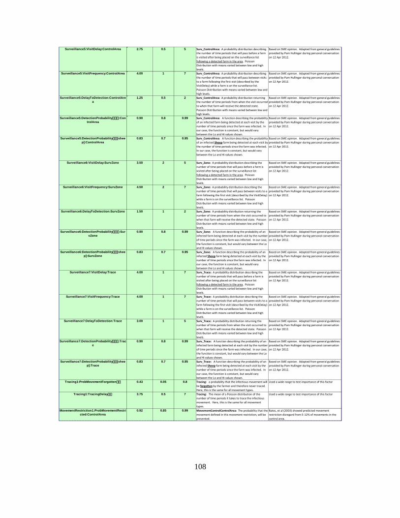
108
Surveillance5:VisitDelay:ControlArea 2.75 0.5 5 Surv_ControlArea: A probability distribution describing
the number of time periods that will pass before a farm
is visited after being placed on the surveillance list
following a detected farm in the area. Poisson
Distribution with means varied between low and high
levels.
Based on SME opinion. Adapted from general guidelines
provided by Pam Hullinger during personal conversation
on 12 Apr 2012.
Surveillance5:VisitFrequency:ControlArea 4.00 1 7 Surv_ControlArea: A probability distribution describing
the number of time periods that will pass between visits
to a farm following the first visit (described by the
VisitDelay) while a farm is on the surveillance list.
Poisson Distribution with means varied between low and
high levels.
Based on SME opinion. Adapted from general guidelines
provided by Pam Hullinger during personal conversation
on 12 Apr 2012.
Surveillance5:DelayToDetection:ControlArea
1.25 0.5 2 Surv_ControlArea: A probability distribution returning
the number of time periods from when the visit occurred
to when that farm will receive the detected state.
Poisson Distribution with means varied between low and
high levels.
Based on SME opinion. Adapted from general guidelines
provided by Pam Hullinger during personal conversation
on 12 Apr 2012.
Surveillance5:DetectionProbability[][][]:ControlArea
0.90 0.8 0.99 Surv_ControlArea: A function describing the probability
of an infected farm being detected at each visit by the
number of time periods since the farm was infected. In
our case, the function is constant, but would vary
between the Lo and Hi values shown.
Based on SME opinion. Adapted from general guidelines
provided by Pam Hullinger during personal conversation
on 12 Apr 2012.
Surveillance5:DetectionProbability[][][sheep]:ControlArea
0.83 0.7 0.95 Surv_ControlArea: A function describing the probability
of an infected Sheep farm being detected at each visit by
the number of time periods since the farm was infected.
In our case, the function is constant, but would vary
between the Lo and Hi values shown.
Based on SME opinion. Adapted from general guidelines
provided by Pam Hullinger during personal conversation
on 12 Apr 2012.
Surveillance6:VisitDelay:SurvZone 3.50 2 5 Surv_Zone: A probability distribution describing the
number of time periods that will pass before a farm is
visited after being placed on the surveillance list
following a detected farm in the area. Poisson
Distribution with means varied between low and high
levels.
Based on SME opinion. Adapted from general guidelines
provided by Pam Hullinger during personal conversation
on 12 Apr 2012.
Surveillance6:VisitFrequency:SurvZone 4.50 2 7 Surv_Zone: A probability distribution describing the
number of time periods that will pass between visits to a
farm following the first visit (described by the VisitDelay)
while a farm is on the surveillance list. Poisson
Distribution with means varied between low and high
levels.
Based on SME opinion. Adapted from general guidelines
provided by Pam Hullinger during personal conversation
on 12 Apr 2012.
Surveillance6:DelayToDetection:SurvZone 1.50 1 2 Surv_Zone: A probability distribution returning the
number of time periods from when the visit occurred to
when that farm will receive the detected state. Poisson
Distribution with means varied between low and high
levels.
Based on SME opinion. Adapted from general guidelines
provided by Pam Hullinger during personal conversation
on 12 Apr 2012.
Surveillance6:DetectionProbability[][][]:SurvZone
0.90 0.8 0.99 Surv_Zone: A function describing the probability of an
infected farm being detected at each visit by the number
of time periods since the farm was infected. In our case,
the function is constant, but would vary between the Lo
and Hi values shown.
Based on SME opinion. Adapted from general guidelines
provided by Pam Hullinger during personal conversation
on 12 Apr 2012.
Surveillance6:DetectionProbability[][][sheep]:SurvZone
0.83 0.7 0.95 Surv_Zone: A function describing the probability of an
infected Sheep farm being detected at each visit by the
number of time periods since the farm was infected. In
our case, the function is constant, but would vary
between the Lo and Hi values shown.
Based on SME opinion. Adapted from general guidelines
provided by Pam Hullinger during personal conversation
on 12 Apr 2012.
Surveillance7:VisitDelay:Trace 4.00 1 7 Surv_Trace: A probability distribution describing the
number of time periods that will pass before a farm is
visited after being placed on the surveillance list
following a detected farm in the area. Poisson
Distribution with means varied between low and high
levels.
Based on SME opinion. Adapted from general guidelines
provided by Pam Hullinger during personal conversation
on 12 Apr 2012.
Surveillance7:VisitFrequency:Trace 4.00 1 7 Surv_Trace: A probability distribution describing the
number of time periods that will pass between visits to a
farm following the first visit (described by the VisitDelay)
while a farm is on the surveillance list. Poisson
Distribution with means varied between low and high
levels.
Based on SME opinion. Adapted from general guidelines
provided by Pam Hullinger during personal conversation
on 12 Apr 2012.
Surveillance7:DelayToDetection:Trace 3.00 1 5 Surv_Trace: A probability distribution returning the
number of time periods from when the visit occurred to
when that farm will receive the detected state. Poisson
Distribution with means varied between low and high
levels.
Based on SME opinion. Adapted from general guidelines
provided by Pam Hullinger during personal conversation
on 12 Apr 2012.
Surveillance7:DetectionProbability[][][]:Trace
0.90 0.8 0.99 Surv_Trace: A function describing the probability of an
infected farm being detected at each visit by the number
of time periods since the farm was infected. In our case,
the function is constant, but would vary between the Lo
and Hi values shown.
Based on SME opinion. Adapted from general guidelines
provided by Pam Hullinger during personal conversation
on 12 Apr 2012.
Surveillance7:DetectionProbability[][][sheep]:Trace
0.83 0.7 0.95 Surv_Trace: A function describing the probability of an
infected Sheep farm being detected at each visit by the
number of time periods since the farm was infected. In
our case, the function is constant, but would vary
between the Lo and Hi values shown.
Based on SME opinion. Adapted from general guidelines
provided by Pam Hullinger during personal conversation
on 12 Apr 2012.
Tracing1:ProbMovementForgotten[][] 0.43 0.05 0.8 Tracing: a probability that the infectious movement will
be forgotten by the farmer and therefore never traced.
Here, this is the same for all movement types.
Used a wide range to test importance of this factor
Tracing1:TracingDelay[][] 3.75 0.5 7 Tracing: The mean of a Poisson distribution of the
number of time periods it takes to trace the infectious
movement. Here, this is the same for all movement
types.
Used a wide range to test importance of this factor
MovementRestriction1:ProbMovementRestricted:ControlArea
0.92 0.85 0.99 MovementControlControlArea: The probability that the
movement defined in this movement restriction, will be
prevented.
Bates, et al (2003) showed predicted movement
restriction disregard from 5‐12% of movements in the
control area.

109
MovementRestriction2:ProbMovementRestricted:SurvZone
0.85 0.7 0.99 MovementControl_Surv: The probability that the
movement defined in this movement restriction, will be
prevented.
Bates, et al (2003). We estimated that restrictions
outside of the control area may be disregarded at a
higher percentage than within the control area.
Vaccination1:FarmClasses:DairyOnly 0 1 Vacc_Zone: Binary. If 0, then all cattle will be
vaccinated. If 1, only Dairy premises, Dairy calf ranches,
and feedlots will be vaccinated.
Based on SME opinion. Adapted from general guidelines
provided by Pam Hullinger during personal conversation
on 12 Apr 2012. If there is a 1 here, this then applies to
farm types ("31 | 32 | 33 | 51 | 53 | 73").
MovementRestriction3:ProbMovementRestricted:StopMarkets
0 0.995 StopMarkets: Binary variable defining the movement
restrictions put on the market will be set for all
markets (hi value) or only markets in a control area or
surveillance zone.
Tests whether shutting down all markets or only those in
the control area is a better strategy.
Binary Variables

110
THIS PAGE INTENTNIONALLY LEFT BLANK
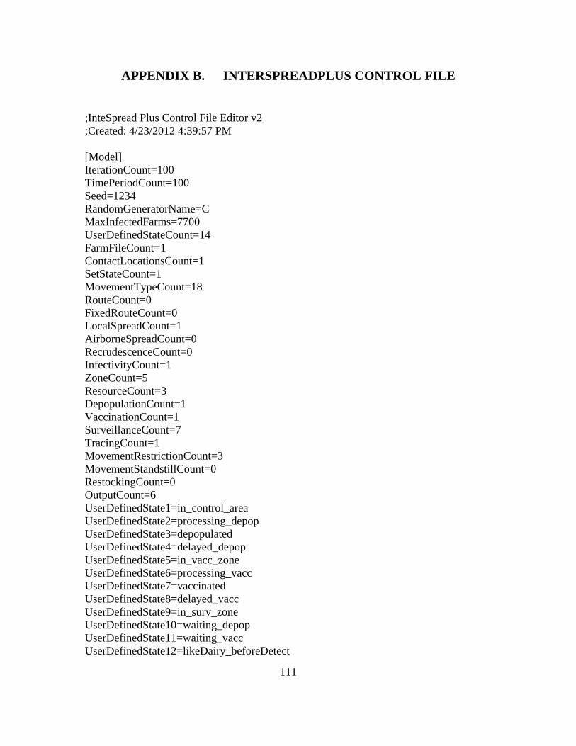
111
APPENDIX B. INTERSPREADPLUS CONTROL FILE
;InteSpread Plus Control File Editor v2 ;Created: 4/23/2012 4:39:57 PM [Model] IterationCount=100 TimePeriodCount=100 Seed=1234 RandomGeneratorName=C MaxInfectedFarms=7700 UserDefinedStateCount=14 FarmFileCount=1 ContactLocationsCount=1 SetStateCount=1 MovementTypeCount=18 RouteCount=0 FixedRouteCount=0 LocalSpreadCount=1 AirborneSpreadCount=0 RecrudescenceCount=0 InfectivityCount=1 ZoneCount=5 ResourceCount=3 DepopulationCount=1 VaccinationCount=1 SurveillanceCount=7 TracingCount=1 MovementRestrictionCount=3 MovementStandstillCount=0 RestockingCount=0 OutputCount=6 UserDefinedState1=in_control_area UserDefinedState2=processing_depop UserDefinedState3=depopulated UserDefinedState4=delayed_depop UserDefinedState5=in_vacc_zone UserDefinedState6=processing_vacc UserDefinedState7=vaccinated UserDefinedState8=delayed_vacc UserDefinedState9=in_surv_zone UserDefinedState10=waiting_depop UserDefinedState11=waiting_vacc UserDefinedState12=likeDairy_beforeDetect

112
UserDefinedState13=likeDairy_afterDetect UserDefinedState14=likeDairy [FarmFile1] Pathname=.\CalFarmFinal_withDensity.txt NumberOfColumns=17 Column1=farmid Column2=farm_class Column3=user_defined FIPS_Code long Column4=user_defined UTM_Zone double Column5=animals cattle Column6=animals swine Column7=animals sheep Column8=animals goat Column9=animals other Column10=user_defined Type_Name string Column11=user_defined premise_3k long Column12=user_defined premise_10k long Column13=user_defined premise_20k long Column14=user_defined animal_3k long Column15=user_defined animal_10k long Column16=user_defined animal_20k long Column17=coordinates [ContactLocations1] ContactLocationsName=Markets_Combined Pathname=.\CAMarket_combined.txt [EpidemicHistory] StateFileName=.\STATE_Port_LA11.txt HistoryEndTimePeriod=1 InfectedFarmHandling=include_always [SetState1] TimePeriod=1 Coordinates=.\ZoneCalUTM.txt FarmClasses=31 | 32 | 33 | 51 | 53 | 73 ProportionOfFarms=1.0 StatesToSet=likeDairy [MovementType1] MovementName=Movement_Farm_Farm_Backyard TimePeriodStart=1 TimePeriodStop=1000 NumberPerTimePeriod=Constant 0
113
NumberOfDirectContacts=Constant 1 DestinationType=farm MovementDistance=1,0,0.615,0.11,0.025,0.06,0.01,0.035,0.01,0,0.135;0,0,19000,39000,59000,79000,99000,119000,139000,159000,179000 ProbabilityOfTransmission=Constant 0.2 NumberPerTimePeriod[114|214|314|24|34]=Poisson 0.049 [MovementType2] MovementName=Movement_Farm_Farm_Goat TimePeriodStart=1 TimePeriodStop=1000 NumberPerTimePeriod=Constant 0 NumberOfDirectContacts=Constant 1 DestinationType=farm MovementDistance=1,0,0.365,0.16,0.09,0.035,0.01,0,0.015,0.025,0.3;0,0,19000,39000,59000,79000,99000,119000,139000,159000,179000 ProbabilityOfTransmission=Constant 0.2 NumberPerTimePeriod[310]=Poisson 0.115 [MovementType3] MovementName=Movement_Farm_Farm_Sheep TimePeriodStart=1 TimePeriodStop=1000 NumberPerTimePeriod=Constant 0 NumberOfDirectContacts=Constant 1 DestinationType=farm MovementDistance=1,0,0.365,0.16,0.09,0.035,0.01,0,0.015,0.025,0.3;0,0,19000,39000,59000,79000,99000,119000,139000,159000,179000 ProbabilityOfTransmission=Constant 0.2 NumberPerTimePeriod[211|213]=Poisson 0.154 [MovementType4] MovementName=Movement_Farm_Farm_BeefS TimePeriodStart=1 TimePeriodStop=1000 NumberPerTimePeriod=Constant 0 NumberOfDirectContacts=Constant 1 DestinationType=farm MovementDistance=1,0,0.39,0.22,0.125,0.055,0.025,0.01,0.02,0.015,0.14;0,0,19000,39000,59000,79000,99000,119000,139000,159000,179000 ProbabilityOfTransmission=Constant 0.338 NumberPerTimePeriod[51|61]=Poisson 0.02 [MovementType5] MovementName=Movement_Farm_Farm_BeefL

114
TimePeriodStart=1 TimePeriodStop=1000 NumberPerTimePeriod=Constant 0 NumberOfDirectContacts=Constant 1 DestinationType=farm MovementDistance=1,0,0.39,0.22,0.125,0.055,0.025,0.01,0.02,0.015,0.14;0,0,19000,39000,59000,79000,99000,119000,139000,159000,179000 ProbabilityOfTransmission=Constant 0.338 NumberPerTimePeriod[53|63]=Poisson 0.038 [MovementType6] MovementName=Movement_Farm_Farm_DairyS TimePeriodStart=1 TimePeriodStop=1000 NumberPerTimePeriod=Constant 0 NumberOfDirectContacts=Constant 1 DestinationType=farm MovementDistance=1,0,0.57,0.255,0.035,0.01,0.005,0.01,0.005,0.005,0.105;0,0,19000,39000,59000,79000,99000,119000,139000,159000,179000 ProbabilityOfTransmission=Constant 0.338 NumberPerTimePeriod[31|32]=Poisson 0.164 [MovementType7] MovementName=Movement_Farm_Farm_DairyL TimePeriodStart=1 TimePeriodStop=1000 NumberPerTimePeriod=Constant 0 NumberOfDirectContacts=Constant 1 DestinationType=farm MovementDistance=1,0,0.57,0.255,0.035,0.01,0.005,0.01,0.005,0.005,0.105;0,0,19000,39000,59000,79000,99000,119000,139000,159000,179000 ProbabilityOfTransmission=Constant 0.338 NumberPerTimePeriod[33]=Poisson 0.298 [MovementType8] MovementName=Movement_Farm_Farm_Calf_HeiferS TimePeriodStart=1 TimePeriodStop=1000 NumberPerTimePeriod=Constant 0 NumberOfDirectContacts=Constant 1 DestinationType=farm MovementDistance=1,0,0.41,0.145,0.205,0,0,0,0.02,0,0.22;0,0,19000,39000,59000,79000,99000,119000,139000,159000,179000 ProbabilityOfTransmission=Constant 0.338 NumberPerTimePeriod[41]=Poisson 0.017
115
[MovementType9] MovementName=Movement_Farm_Farm_Calf_HeiferL TimePeriodStart=1 TimePeriodStop=1000 NumberPerTimePeriod=Constant 0 NumberOfDirectContacts=Constant 1 DestinationType=farm MovementDistance=1,0,0.41,0.145,0.205,0,0,0,0.02,0,0.22;0,0,19000,39000,59000,79000,99000,119000,139000,159000,179000 ProbabilityOfTransmission=Constant 0.338 NumberPerTimePeriod[43|73]=Poisson 0.657 [MovementType10] MovementName=Movement_Farm_Farm_SwineS TimePeriodStart=1 TimePeriodStop=1000 NumberPerTimePeriod=Constant 0 NumberOfDirectContacts=Constant 1 DestinationType=farm MovementDistance=1,0,0.315,0.29,0.02,0.05,0.12,0.045,0.015,0,0.145;0,0,19000,39000,59000,79000,99000,119000,139000,159000,179000 ProbabilityOfTransmission=Constant 0.9999 NumberPerTimePeriod[121|131|151|161]=Poisson 0.088 [MovementType11] MovementName=Movement_Farm_Farm_SwineL TimePeriodStart=1 TimePeriodStop=1000 NumberPerTimePeriod=Constant 0 NumberOfDirectContacts=Constant 1 DestinationType=farm MovementDistance=1,0,0.315,0.29,0.02,0.05,0.12,0.045,0.015,0,0.145;0,0,19000,39000,59000,79000,99000,119000,139000,159000,179000 ProbabilityOfTransmission=Constant 0.9999 NumberPerTimePeriod[153|163]=Poisson 0.334 [MovementType12] MovementName=Movement_market-farm TimePeriodStart=1 TimePeriodStop=1000 NumberPerTimePeriod=Constant 0 NumberOfDirectContacts=Constant 0 DestinationType=farm RestrictOnAnimals=N

116
MovementDistance=1,0,0.383,0.202,0.119,0.061,0.013,0.069,0.04,0.021,0.092;0,0,19000,39000,59000,79000,99000,119000,139000,159000,179000 ProbabilityOfTransmission=Constant 0.8 MaxResampleAttempts=0 [MovementType13] MovementName=Movement_farm-market TimePeriodStart=1 TimePeriodStop=1000 NumberPerTimePeriod=Poisson 0.1 NumberOfDirectContacts=Constant 1 DestinationType=contact_location ContactLocationControlName=Markets_Combined RestrictOnAnimals=N MovementDistance=1,0,0.546,0.216,0.167,0.018,0.005,0.014,0.004,0.006,0.024;0,0,19000,39000,59000,79000,99000,119000,139000,159000,179000 ProbabilityOfTransmission=Constant 0.8 MaxResampleAttempts=0 SourceOfSecondaryContacts=source NumberOfSecondaryContacts[Movement_market-farm]=Poisson 1 [MovementType14] MovementName=IDMovement_Size1 TimePeriodStart=1 TimePeriodStop=1000 NumberPerTimePeriod=Constant 0 NumberOfDirectContacts=Constant 1 DestinationType=farm MovementDistance=1,0,0.44,0.3283,0.1367,0.055,0.011,0.029;0,0,9000,19000,29000,39000,49000,59000 ProbabilityOfTransmission=Constant 0.338 NumberPerTimePeriod[41]=Poisson 0.005 [MovementType15] MovementName=IDMovement_Size2 TimePeriodStart=1 TimePeriodStop=1000 NumberPerTimePeriod=Constant 0 NumberOfDirectContacts=Constant 1 DestinationType=farm MovementDistance=1,0,0.44,0.3283,0.1367,0.055,0.011,0.029;0,0,9000,19000,29000,39000,49000,59000 ProbabilityOfTransmission=Constant 0.338 NumberPerTimePeriod[24|34|114|214|314|310|211|213|51|61|53|63|121|131|151|161]=Poisson 0.0252

117
[MovementType16] MovementName=IDMovement_Size3 TimePeriodStart=1 TimePeriodStop=1000 NumberPerTimePeriod=Constant 0 NumberOfDirectContacts=Constant 1 DestinationType=farm MovementDistance=1,0,0.44,0.3283,0.1367,0.055,0.011,0.029;0,0,9000,19000,29000,39000,49000,59000 ProbabilityOfTransmission=Constant 0.338 NumberPerTimePeriod[153|163]=Poisson 0.1853 [MovementType17] MovementName=IDMovement_Size4 TimePeriodStart=1 TimePeriodStop=1000 NumberPerTimePeriod=Constant 0 NumberOfDirectContacts=Constant 1 DestinationType=farm MovementDistance=1,0,0.44,0.3283,0.1367,0.055,0.011,0.029;0,0,9000,19000,29000,39000,49000,59000 ProbabilityOfTransmission=Constant 0.338 NumberPerTimePeriod[31|32|43|73]=Poisson .4294 [MovementType18] MovementName=IDMovement_Size5 TimePeriodStart=1 TimePeriodStop=1000 NumberPerTimePeriod=Constant 0 NumberOfDirectContacts=Constant 1 DestinationType=farm MovementDistance=1,0,0.44,0.3283,0.1367,0.055,0.011,0.029;0,0,9000,19000,29000,39000,49000,59000 ProbabilityOfTransmission=Constant 0.338 NumberPerTimePeriod[33]=Poisson .9517 [LocalSpread1] TimePeriodStart=1 TimePeriodStop=1000 POTOffsetRelativeTo=clinical_signs ProbabilityOfTransmission=7,1000,2000,3000;-1,0,0,0;0,0.013,0.003,0.001;1,0.039,0.009,0.003;2,0.052,0.012,0.004;3,0.052,0.012,0.004;4,0.052,0.012,0.004;5,0.052,0.012,0.004 RelativeSusceptibility[swine]=0.01

118
RelativeSusceptibility[sheep]=0.05 RelativeSusceptibility[goat]=0.05 RelativeSusceptibility[cattle]=1.0 [Infectivity1] TimePeriodStart=1 TimePeriodStop=1000 TimeToClinicalSigns=Lookup 1,2,3,4,5,6,7,8,9,11,12,16,17;0,0.035,0.158,0.333,0.772,0.789,0.825,0.877,0.912,0.947,0.965,0.982,1 InfectivityRelativeTo=clinical_signs WithinFarmSpreadProb=1.0 Infectivity[][][]=Table 1,16,17,18,19,20,21,22,23,24,25,26,27,28,29,30,31,32,33;0,1,0.941,0.882,0.823,0.764,0.705,0.646,0.587,0.528,0.469,0.41,0.351,0.292,0.233,0.174,0.115,0.056,0 [Zone1] ZoneName=ZoneCalifornia ZoneType=explicit IncludeEntireFarm=N TimePeriodStartReference=simulation_start TimePeriodStopReference=simulation_start ChangeCount=1 TimePeriodStart1=1 TimePeriodStop1=1000 Coordinates1=.\ZoneCalUTM.txt [Zone2] ZoneName=Zone_ControlArea ZoneType=radial FarmState=in_control_area UseFarmCentroid=Y IncludeEntireFarm=N ChangeCount=1 TimePeriodStart1=1 TimePeriodStop1=1000 InsideRadius1=0 OutsideRadius1=3000 [Zone3] ZoneName=Zone_Vaccinate ZoneType=radial FarmState=in_vacc_zone UseFarmCentroid=Y IncludeEntireFarm=N
119
ChangeCount=1 TimePeriodStart1=1 TimePeriodStop1=1000 InsideRadius1=0 OutsideRadius1=3000 [Zone4] ZoneName=Zone_Surv ZoneType=radial FarmState=in_surv_zone UseFarmCentroid=Y IncludeEntireFarm=N ExcludeFarmsInZones=Zone_ControlArea ChangeCount=1 TimePeriodStart1=1 TimePeriodStop1=1000 InsideRadius1=0 OutsideRadius1=3000 [Zone5] ZoneName=Zone_likeDairy ZoneType=explicit FarmState=likeDairy TimePeriodStartReference=simulation_start TimePeriodStopReference=first_detection ChangeCount=1 TimePeriodStart1=1 TimePeriodStop1=1 Coordinates1=.\ZoneCalUTM.txt [Resource1] ResourceName=DepopResource WaitingFarmState=waiting_depop ProcessingFarmState=processing_depop CompletedFarmState=depopulated DelayedFarmState=delayed_depop TimePeriodToDelayedState=1 ActionOption=depopulation FarmListOption=single_list FarmProcessingOption=animals_per_time_period ChangeCount=2 TimePeriodStart1=1 TimePeriodStop1=9 cattlePerTimePeriod1=2000 goatPerTimePeriod1=2000
120
otherPerTimePeriod1=2000 sheepPerTimePeriod1=2000 swinePerTimePeriod1=2000 TimePeriodStart2=10 TimePeriodStop2=1000 cattlePerTimePeriod2=20000 goatPerTimePeriod2=20000 otherPerTimePeriod2=20000 sheepPerTimePeriod2=20000 swinePerTimePeriod2=20000 [Resource2] ResourceName=VaccinationResource WaitingFarmState=waiting_vacc ProcessingFarmState=processing_vacc CompletedFarmState=vaccinated DelayedFarmState=delayed_vacc TimePeriodToDelayedState=1 ActionOption=vaccination FarmListOption=single_list FarmProcessingOption=animals_per_time_period ChangeCount=2 TimePeriodStart1=1 TimePeriodStop1=9 cattlePerTimePeriod1=2000 goatPerTimePeriod1=2000 otherPerTimePeriod1=2000 sheepPerTimePeriod1=2000 swinePerTimePeriod1=2000 TimePeriodStart2=10 TimePeriodStop2=1000 cattlePerTimePeriod2=20000 goatPerTimePeriod2=20000 otherPerTimePeriod2=20000 sheepPerTimePeriod2=20000 swinePerTimePeriod2=20000 [Resource3] ResourceName=SurvResource ActionOption=depopulation SurveillanceControl=Surv_ControlArea FarmListOption=single_list FarmProcessingOption=farms_per_time_period ChangeCount=1 TimePeriodStart1=1

121
TimePeriodStop1=1000 FarmsPerTimePeriod1=0 [Depopulation1] ControlName=Depop_Detected ActivationOption=detected_farm TimePeriodStartReference=simulation_start TimePeriodStopReference=simulation_start FarmSelectionOption=detected_farm ActionResource=DepopResource WaitingFarmState=waiting_depop ProcessingFarmState=processing_depop CompletedFarmState=depopulated DelayedFarmState=delayed_depop TimePeriodToDelayedState=1 [Vaccination1] ControlName=Vacc_Zone ActivationOption=detected_farm TimePeriodStartReference=simulation_start TimePeriodStopReference=simulation_start FarmSelectionOption=zone SelectionZone=Zone_Vaccinate SelectionZoneFarmSortOrder=outer_to_inner FarmClasses=31 | 32 | 33 | 51 | 53 | 73 AnimalTypes=cattle ActionResource=VaccinationResource WaitingFarmState=waiting_vacc ProcessingFarmState=processing_vacc CompletedFarmState=vaccinated DelayedFarmState=delayed_vacc TimePeriodToDelayedState=1 RemoveDetectedFarms=N ImmunityFunction=Table 1,0,4,15;0,0,0.1,0.05 [Surveillance1] ControlName=GeneralSurveillance ActivationOption=time_period TimePeriodStartReference=simulation_start TimePeriodStart=1 TimePeriodStopReference=first_detection TimePeriodStop=1 SelectionZone=ZoneCalifornia SelectionProbability=0.65 VisitDelay=Poisson 2

122
VisitFrequency=Poisson 7 VisitDuration=Constant 1000 DelayToDetection=Poisson 3 DetectionRelativeTo=Clinical_signs DetectionProbability[][][]=Constant 0.95 DetectionProbability[][][sheep]=Constant 0.5 [Surveillance2] ControlName=GeneralSurveillance_AfterDetect ActivationOption=time_period TimePeriodStartReference=first_detection TimePeriodStart=1 TimePeriodStopReference=first_detection TimePeriodStop=1000 SelectionZone=ZoneCalifornia SelectionProbability=0.85 VisitDelay=Poisson 2 VisitFrequency=Poisson 7 VisitDuration=Constant 1000 DelayToDetection=Poisson 3 DetectionRelativeTo=Clinical_signs DetectionProbability[][][]=Constant 0.95 DetectionProbability[][][sheep]=Constant 0.85 [Surveillance3] ControlName=GeneralSurv_Dairy_before ActivationOption=time_period TimePeriodStartReference=simulation_start TimePeriodStart=1 TimePeriodStopReference=first_detection TimePeriodStop=1 SurveillanceFarmState=likeDairy_beforeDetect SelectionZone=Zone_likeDairy SelectionProbability=0.999 VisitDelay=Poisson 1 VisitFrequency=Poisson 2 VisitDuration=Constant 1000 DelayToDetection=Poisson 3 DetectionRelativeTo=Clinical_signs DetectionProbability[][][]=Constant 0.5 [Surveillance4] ControlName=GeneralSurv_Dairy_after ActivationOption=time_period TimePeriodStartReference=first_detection

123
TimePeriodStart=1 TimePeriodStopReference=first_detection TimePeriodStop=1000 SurveillanceFarmState=likeDairy_afterDetect SelectionZone=Zone_likeDairy SelectionProbability=0.999 VisitDelay=Poisson 0.5 VisitFrequency=Poisson 1 VisitDuration=Constant 1000 DelayToDetection=Poisson 1 DetectionRelativeTo=Clinical_signs DetectionProbability[][][]=Constant 0.95 [Surveillance5] ControlName=Surv_ControlArea ActivationOption=detected_farm TimePeriodStartReference=first_detection TimePeriodStart=1 TimePeriodStopReference=first_detection TimePeriodStop=1000 SurveillanceFarmState=in_control_area SelectionZone=Zone_ControlArea SelectionProbability=0.99 VisitDelay=Poisson 2 VisitFrequency=Poisson 3 VisitDuration=Constant 1000 DelayToDetection=Poisson 1 DetectionRelativeTo=Clinical_signs DetectionProbability[][][]=Constant 0.99 DetectionProbability[][][sheep]=Constant 0.9 [Surveillance6] ControlName=Surv_Zone ActivationOption=detected_farm TimePeriodStartReference=first_detection TimePeriodStart=1 TimePeriodStopReference=first_detection TimePeriodStop=1000 SurveillanceFarmState=in_surv_zone SelectionZone=Zone_Surv SelectionProbability=0.9 VisitDelay=Poisson 3 VisitFrequency=Poisson 7 VisitDuration=Constant 1000 DelayToDetection=Poisson 2

124
DetectionRelativeTo=Clinical_signs DetectionProbability[][][]=Constant 0.99 DetectionProbability[][][sheep]=Constant 0.9 [Surveillance7] ControlName=Surv_Trace ActivationOption=time_period TimePeriodStartReference=first_detection TimePeriodStart=1 TimePeriodStopReference=first_detection TimePeriodStop=1000 SelectionZone=ZoneCalifornia SelectionProbability=0.75 VisitDelay=Poisson 2 VisitFrequency=Poisson 5 VisitDuration=Constant 1000 DelayToDetection=Poisson 3 DetectionRelativeTo=Clinical_signs DetectionProbability[][][]=Constant 0.95 DetectionProbability[][][sheep]=Constant 0.85 [Tracing1] ControlName=Tracing TimePeriodStartReference=first_detection TimePeriodStart=2 TimePeriodStopReference=first_detection TimePeriodStop=1000 TracingRequired[][]=Y ProbMovementForgotten[][]=0.2 TracingDelay[][]=Poisson 2 SurveillanceControls[][]=Surv_Trace [MovementRestriction1] ControlName=MovementControlControlArea TimePeriodStartReference=first_detection TimePeriodStart=1 TimePeriodStopReference=first_detection TimePeriodStop=1000 MovementTypes=IDMovement_Size1 IDMovement_Size2 IDMovement_Size3 IDMovement_Size4 IDMovement_Size5 Movement_farm-market Movement_Farm_Farm_Backyard Movement_Farm_Farm_BeefL Movement_Farm_Farm_BeefS Movement_Farm_Farm_Calf_HeiferL Movement_Farm_Farm_Calf_HeiferS Movement_Farm_Farm_DairyL Movement_Farm_Farm_DairyS Movement_Farm_Farm_Goat
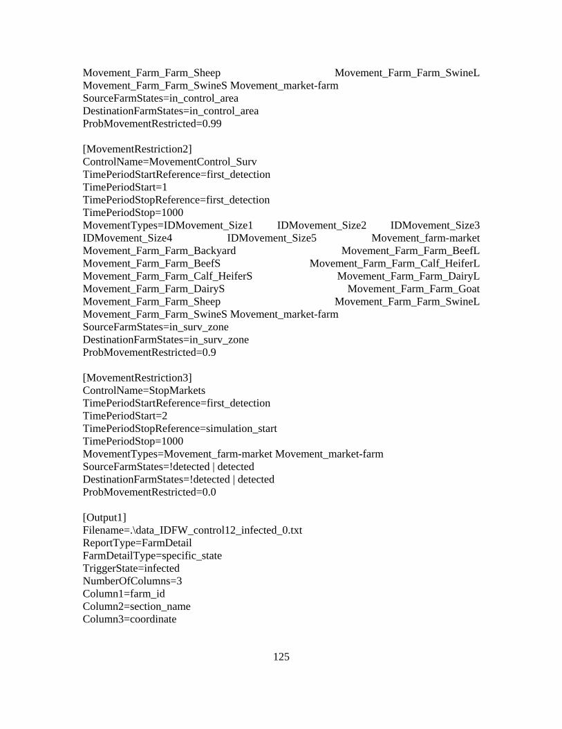
125
Movement_Farm_Farm_Sheep Movement_Farm_Farm_SwineL Movement_Farm_Farm_SwineS Movement_market-farm SourceFarmStates=in_control_area DestinationFarmStates=in_control_area ProbMovementRestricted=0.99 [MovementRestriction2] ControlName=MovementControl_Surv TimePeriodStartReference=first_detection TimePeriodStart=1 TimePeriodStopReference=first_detection TimePeriodStop=1000 MovementTypes=IDMovement_Size1 IDMovement_Size2 IDMovement_Size3 IDMovement_Size4 IDMovement_Size5 Movement_farm-market Movement_Farm_Farm_Backyard Movement_Farm_Farm_BeefL Movement_Farm_Farm_BeefS Movement_Farm_Farm_Calf_HeiferL Movement_Farm_Farm_Calf_HeiferS Movement_Farm_Farm_DairyL Movement_Farm_Farm_DairyS Movement_Farm_Farm_Goat Movement_Farm_Farm_Sheep Movement_Farm_Farm_SwineL Movement_Farm_Farm_SwineS Movement_market-farm SourceFarmStates=in_surv_zone DestinationFarmStates=in_surv_zone ProbMovementRestricted=0.9 [MovementRestriction3] ControlName=StopMarkets TimePeriodStartReference=first_detection TimePeriodStart=2 TimePeriodStopReference=simulation_start TimePeriodStop=1000 MovementTypes=Movement_farm-market Movement_market-farm SourceFarmStates=!detected | detected DestinationFarmStates=!detected | detected ProbMovementRestricted=0.0 [Output1] Filename=.\data_IDFW_control12_infected_0.txt ReportType=FarmDetail FarmDetailType=specific_state TriggerState=infected NumberOfColumns=3 Column1=farm_id Column2=section_name Column3=coordinate

126
[Output2] Filename=.\data_IDFW_control12_in_control_area_0.txt ReportType=FarmDetail FarmDetailType=specific_state TriggerState=in_control_area NumberOfColumns=1 Column1=farm_id [Output3] Filename=.\data_IDFW_control12_in_vacc_zone_0.txt ReportType=FarmDetail FarmDetailType=specific_state TriggerState=in_vacc_zone NumberOfColumns=1 Column1=farm_id [Output4] Filename=.\data_IDFW_control12_in_surv_zone_0.txt ReportType=FarmDetail FarmDetailType=specific_state TriggerState=in_surv_zone NumberOfColumns=1 Column1=farm_id [Output5] Filename=.\data_IDFW_control12_depopulated_0.txt ReportType=FarmDetail FarmDetailType=specific_state TriggerState=depopulated NumberOfColumns=1 Column1=farm_id [Output6] Filename=.\data_IDFW_control12_detected_0.txt ReportType=FarmDetail FarmDetailType=specific_state TriggerState=detected NumberOfColumns=2 Column1=farm_id Column2=section_name ;Checksum=1760877

127
LIST OF REFERENCES
Bates, T. W., Thurmond, M. C., & Carpenter, T. E. (2001). Direct and indirect contact rates among beef, dairy, goat, sheep, and swine herds in three California counties, with reference to control of potential foot-and-mouth disease transmission. American Journal of Veterinary Research, 62(7), 1121–1129.
Box, G. E. P., & Cox, D. R. (1964). An analysis of transformations. Journal of the Royal Statistical Society. Series B (Methodological), 211–252.
California Department of Food and Agriculture (CDFA). (2006). Mobilization plan for emergency animal disease of livestock. Retrieved from http://www.cdfa.ca.gov/ ahfss/Animal_Health/pdfs/Overview_FAD_Response_1.pdf
California Department of Transportation (Caltrans). (1993). California Department of Transportation LS/LSIT exam preparation course. Retrieved from http://www.dot.ca.gov/hq/row/landsurveys/LSITWorkbook/WorkbookTOC.html
Carpenter, T. E., Christiansen, L. E., Dickey, B. F., Thunes, C., & Hullinger, P. J. (2007). Potential impact of an introduction of foot-and-mouth disease into the california state fair. Journal of the American Veterinary Medical Association, 231(8), 1231–1235.
Carpenter, T. E., O’Brien, J. M., Hagerman, A. D., & McCarl, B. A. (2011). Epidemic and economic impacts of delayed detection of foot-and-mouth disease: A case study of a simulated outbreak in California. Journal of Veterinary Diagnostic Investigation, 23(1), 26–33.
Cioppa, T. M., & Lucas, T. W. (2007). Efficient nearly orthogonal and space-filling Latin hypercubes. Technometrics, 49(1), 45–55.
Doel, T., Williams, L., & Barnett, P. (1994). Emergency vaccination against foot-and-mouth disease: Rate of development of immunity and its implications for the carrier state. Vaccine, 12(7), 592–600
Donaldson, A., Alexandersen, S., Sorensen, J., & Mikkelsen, T. (2001). Relative risks of the uncontrollable (airborne) spread of FMD by different species. Veterinary Record, 148(19), 602–604.
Dubé, C. (2009). Network analysis of dairy cattle movements in Ontario to support livestock disease simulation modelling (Doctoral dissertation). The University of Guelph, Ontario, Canada.
128
Dubé, C. et al. (2007). The use of epidemiological models for the management of animal diseases. Report to 75th General Session, World Organization for Animal Health. Retrieved from http://www.mattilsynet.no/mattilsynet/ multimedia/archive/00029/A_75SG_9_1__29995a.pdf
Garner, M., & Beckett, S. (2005). Modelling the spread of foot‐and‐mouth disease in Australia. Australian Veterinary Journal, 83(12), 758–766.
Gibbens, J., & Wilesmith, J. (2002). Temporal and geographical distribution of cases of foot-and-mouth disease during the early weeks of the 2001 epidemic in Great Britain. Veterinary Record, 151(14), 407–412.
Hagerman, A. D., McCarl, B. A., Carpenter, T., & O’Brien, J. (2009, October 30). Impact of foot-and-mouth disease management alternatives in the California dairy industry. Foreign Animal and Zoonotic Disease Defense (FAZD) Center, Texas A&M University. Retrieved from http://agecon2.tamu.edu/people/faculty/ mccarl-bruce/papers/1832DADS-ASM_Report10-09.pdf
Harvey, N. et al. (2007). The North American animal disease spread model: A simulation model to assist decision making in evaluating animal disease incursions. Preventive Veterinary Medicine, 82, 176–197.
Hullinger, P. (2012). Personal communication in reference to Melius et al. update and parameters settings to be used in InterSpreadPlus to model the spread and control of an outbreak of FMD in California.
JMP® Pro, Version 9.0.3. SAS Institute Inc., Cary, NC, 1989–2012.
Keeling, M. J. (2005). Models of foot-and-mouth disease. Proceedings of the Royal Society B: Biological Sciences, 272(1569), 1195–1202.
Knowles, N.J. (1990). Molecular and antigenic variation of foot-and-mouth disease virus. M.Phil Thesis, March, 1990, Council for National Academic Awards. Retrieved from http://www.picornaviridae.com/aphthovirus/fmdv/ fmd_history.htm
Kobayashi, M., Carpenter, T. E., Dickey, B. F., & Howitt, R. E. (2007). A dynamic, optimal disease control model for foot-and-mouth disease: I. model description. Preventive Veterinary Medicine, 79(2), 257–273.
Kostova-Vassilevska, T., Consultants, L., Bates, T., Thurmond, M., & Carpenter, T. (2004). On the use of models to assess foot-and-mouth disease transmission and control. United States Department of Energy.
129
Mardones, F., Perez, A., Sanchez, J., Alkhamis, M., & Carpenter, T. (2010). Parameterization of the duration of infection stages of serotype O foot-and-mouth disease virus: An analytical review and meta-analysis with application to simulation models. Veterinary Research, 41(4).
Massey University. (2008). InterSpreadPlus model description. Retrieved from http://www.interspreadplus.com/info.asp
Matsumoto, M., & Nishimura, T. (1998). Mersenne twister: A 623-dimensionally equidistributed uniform pseudo-random number generator. ACM Transactions on Modeling and Computer Simulation (TOMACS), 8(1), 3–30.
McLaws, M., & Ribble, C. (2007). Description of recent foot and mouth disease outbreaks in nonendemic areas: Exploring the relationship between early detection and epidemic size. The Canadian Veterinary Journal, 48(10), 1051.
Melius, C., Robertson, A., & Hullinger, P. (2006). Developing livestock facility type information from USDA agricultural census data for use in epidemiological and economic models. Department of Homeland Security, Lawrence Livermore National Laboratory, UCRL-TR-226008.
Mendenhall, W., & Sincich, T. (1984). Statistics for the engineering and computer sciences. San Francisco: Dellen Publishing Company.
Montgomery, D. C., Peck, E. A., & Vining, G. G. (2006). Introduction to linear regression analysis. New Jersey: John Wiley & Sons.
Morris, R. (2008). Spatial modelling of animal disease on real world geography using interspread plus. Slide presentation, Massey University, Palmerston North, New Zealand.
National Science and Technology Council (NSTC). (2007). Protecting against high consequence animal diseases: Research & development plan for 2008-2012. Retrieved from http://www.whitehouse.gov/sites/default/files/microsites/ostp/ fadt_rd_16_feb_2007.pdf
Orsel, K., Bouma, A., Dekker, A., Stegeman, J., & De Jong, M. (2009). Foot and mouth disease virus transmission during the incubation period of the disease in piglets, lambs, calves, and dairy cows. Preventive Veterinary Medicine, 88(2), 158–163.
Pineda-Krch, M., O’Brien, J. M., Thunes, C., & Carpenter, T. E. (2010). Potential impact of introduction of foot-and-mouth disease from wild pigs into commercial livestock premises in California. American Journal of Veterinary Research, 71(1), 82–88.

130
Posada, D., & Buckley, T. R. (2004). Model selection and model averaging in phylogenetics: Advantages of Akaike information criterion and bayesian approaches over likelihood ratio tests. Systematic Biology, 53(5), 793–808.
R Development Core Team. (2012). R: A language and environment for statistical computing. R Foundation for Statistical Computing, Vienna, Austria. ISBN 3-900051-07-0, URL http://www.R-project.org/.
Sanchez, S. M. (2000). Robust design: Seeking the best of all possible worlds. Proceedings of the 2000 Winter Simulation Conference, Miami, FL.
Sanchez, S. (2008). Better than a petaflop: The Power of efficient experimental design. Proceedings of the 2008 Winter Simulation Conference, Miami, FL. Retrieved from http://or.nps.edu/oa4333/handouts/BetterThanPetaflop_wsc08.pdf
Sanson, R. L., Stevenson, M. A., & Moles-Benfell, N. (2006, August). Quantifying local spread probabilities for foot-and-mouth disease. International Symposia on Veterinary Epidemiology and Economics (ISVEE) proceedings, ISVEE 11: Proceedings of the 11th Symposium of the International Society for Veterinary Epidemiology and Economics, Cairns, Australia, Theme 4 - Tools & training for epidemiologists: Simulation modelling session, p. 681.
Sanson, R. L., Stevenson, M. A., Mackereth, G. F., & Moles-Benfell, N. (2006, August)). The development of an interspread plus parameter set to simulate the spread of FMD in New Zealand. International Symposia on Veterinary Epidemiology and Economics (ISVEE) proceedings, ISVEE 11: Proceedings of the 11th Symposium of the International Society for Veterinary Epidemiology and Economics, Cairns, Australia, Theme 4 - Tools & training for epidemiologists: Simulation modelling session, p. 682.
SAS Institute Inc. (2010). JMP® 9, Modeling and multivariate methods. Cary, NC: SAS Institute Inc.
Stevenson, M. (2012). Personal communication in reference to parameters settings to be used in InterSpreadPlus to model multiple FMD virus types.
Sutmoller, P., Barteling, S. S., Olascoaga, R. C., & Sumption, K. J. (2003). Control and eradication of foot-and-mouth disease. Virus Research, 91(1), 101–144.
U.S. Animal Health Association (USAHA). (2008). Foreign animal diseases, Seventh Edition. Retrieved from http://www.usaha.org/Portals/6/Publications/FAD.pdf
U.S. Department of Agriculture (USDA). (2011). Quarantine, movement control, and continuity of business for a foot-and-mouth disease (fmd) outbreak: Ready reference guide. Retrieved from https://fadprep.lmi.org/Ready%20Reference% 20Guides/COB_RRG_Nov1_FINAL_formeeting_v2.pdf
131
U.S. General Accounting Office (GAO). (2002). Foot and mouth disease: To protect US livestock, USDA must remain vigilant and resolve outstanding issues. Report to the honorable Tom Daschle, U.S. Senate.
United States Department of Agriculture National Agricultural Statistics Service (NASS), (2010). State agricultural overview: California. Retrieved from http://www.nass.usda.gov/Statistics_by_State/Ag_Overview/AgOverview_CA.pdf
Vieira, Jr., H. (2012). NOB_Mixed_512DP_template_v1.xls design spreadsheet. Retrieved from http://harvest.nps.edu
Vieira, Jr., H., Sanchez, S. M., Kienitz, K. H., & Belderrain, M. C. N. (2012). Conducting trade-off analyses via simulation: Efficient nearly orthogonal nearly balanced mixed designs. Working paper, Operations Research Department, Naval Postgraduate School, Monterey, CA.
World Organisation for Animal Health (OIE). (2012). Map developed online using the World Animal Health Information Database (WAHID) Interface. Retrieved from http://web.oie.int/wahis/public.php?page=disease_outbreak_map
Yoon, H. et al. (2006). Simulation analyses to evaluate alternative control strategies for the 2002 foot-and-mouth disease outbreak in the Republic of Korea. Preventive Veterinary Medicine, 74(2), 212–225.

132
THIS PAGE INTENTIONALLY LEFT BLANK

133
INITIAL DISTRIBUTION LIST
1. Defense Technical Information Center Ft. Belvoir, Virginia 2. Dudley Knox Library Naval Postgraduate School Monterey, California 3. John Rowden Program Manager
Department of Food and Agriculture Animal Health and Food Safety Services Emergency Preparedness and Support Unit Sacramento, California
4. Norma Schroeder Emergency: Training, Exercise, & Continuity Planning California Department of Food and Agriculture Sacramento, California
5. Pamela J Hullinger, DVM, MPVM, DACVPM Davis, California
6. Mark Stevenson Institute of Veterinary, Animal and Biomedical Sciences Massey University, Palmerston, North New Zealand
7. Kent Fowler, DVM Sacramento, California 8. Dr. Annette Whiteford (Chief Veterinarian)
California Department of Food and Agriculture Sacramento, California
Recommended