METHODOLOGIES AND APPLICATION
Optimal job scheduling in grid computing using efficient binaryartificial bee colony optimization
Sung-Soo Kim • Ji-Hwan Byeon • Hongbo Liu •
Ajith Abraham • Sean McLoone
Published online: 20 November 2012
� Springer-Verlag Berlin Heidelberg 2012
Abstract The artificial bee colony has the advantage of
employing fewer control parameters compared with other
population-based optimization algorithms. In this paper a
binary artificial bee colony (BABC) algorithm is developed
for binary integer job scheduling problems in grid com-
puting. We further propose an efficient binary artificial bee
colony extension of BABC that incorporates a flexible
ranking strategy (FRS) to improve the balance between
exploration and exploitation. The FRS is introduced to
generate and use new solutions for diversified search in
early generations and to speed up convergence in latter
generations. Two variants are introduced to minimize the
makepsan. In the first a fixed number of best solutions is
employed with the FRS while in the second the number of
the best solutions is reduced with each new generation.
Simulation results for benchmark job scheduling problems
show that the performance of our proposed methods is
better than those alternatives such as genetic algorithms,
simulated annealing and particle swarm optimization.
Keywords Artificial bee colony (ABC) �Binary artificial bee colony (BABC) �Efficient binary artificial bee colony (EBABC) �Flexible ranking strategy (FRS) � Job scheduling �Grid computing
1 Introduction
A computational grid is a large scale, heterogeneous col-
lection of autonomous systems, geographically distributed
and interconnected by low-latency and high-bandwidth
networks (Foster and Kesselman 2004). It provides the
underlying infrastructure for the rapidly growing field of
cloud computing (Foster et al. 2008; Wei and Blake 2010).
The sharing of computational jobs is a major application
for grids. In a computational grid, resources are dynamic
and diverse and can be added and withdrawn at any time at
the owner’s discretion, and their performance or load can
change frequently over time. Grid resource management
provides functionality for the discovery and publishing of
resources as well as scheduling, submission and monitoring
of jobs. Scheduling is a particularly challenging problem as
Communicated by F. Herrera.
S.-S. Kim � J.-H. Byeon
Department of Industrial Engineering, Kangwon National
University, Chunchon 200-701, Korea
e-mail: [email protected]
J.-H. Byeon
e-mail: [email protected]
H. Liu (&)
School of Information Science and Technology, Dalian Maritime
University, Dalian 116026, China
e-mail: [email protected]
H. Liu
Institute for Neural Computation, University of California San
Diego, La Jolla, CA 92093, USA
A. Abraham
Machine Intelligence Research Labs, Scientific Network for
Innovation and Research Excellence, Auburn, WA 98071, USA
e-mail: [email protected]
A. Abraham
IT For Innovations - Center of Excellence, VSB - Technical
University of Ostrava, Ostrava - Poruba 708 33, Czech Republic
S. McLoone
Department of Electronic Engineering, National University of
Ireland Maynooth, Maynooth, Kildare, Ireland
e-mail: [email protected]
123
Soft Comput (2013) 17:867–882
DOI 10.1007/s00500-012-0957-7
it is known to be NP-complete (Garey and Johnson 1979).
Dong and Akl (2006) provide a detailed analysis of the
scheduling problem as it pertains to the grid.
Swarm intelligence is an innovatively distributed intel-
ligent paradigm whereby the intelligence that emerges in
nature from the collective behaviours of unsophisticated
individuals interacting locally with their environment is
exploited to develop optimization algorithms that identify
optimum solutions efficiently in complex search spaces
(Bonabeau et al. 1999; Kennedy et al. 2001; Liu et al.
2007). Within this paradigm algorithms have been devel-
oped that mimic swarming behaviours observed in flocks of
birds, schools of fish, or swarms of bees, colonies of ants
and even human social behaviour, from which intelligence
is seen to emerge (Clerc 2006; Walker 2007; Forestiero
et al. 2008; Su et al. 2009; Banks et al. 2009; Singh and
Sundar 2011; Yang 2011; Cuevas et al. 2012; Abraham
et al. 2012; Yue et al. 2012). Recently, these algorithms
have been investigated as a means of efficiently estimating
optimal job allocation on computational grids in applica-
tion-level scheduling (Abraham et al. 2008; Izakian et al.
2010; Liu et al. 2010).
In this paper we introduce the efficient binary artificial
bee colony (EBABC) algorithm as an enhancement of the
binary artificial bee colony (BABC) algorithm (Pampara
and Engelbrecht 2011; Chandrasekaran et al. 2012) for
solving the makespan minimization problem in grid com-
puting job scheduling (an NP-complete problem). We
demonstrate theoretically that the proposed algorithm
converges with a probability of 1 towards the global opti-
mal and with the aid of benchmark job scheduling prob-
lems illustrate its operation and performance.
The rest of the paper is organized as follows: Section 2
describes related work on swarm intelligence based
approaches to optimal job scheduling. Section 3 deals with
some theoretical foundations related to job scheduling in
grid computing. In Sect. 4, we describe the proposed
EBABC algorithm in detail. Experimental results and
analysis are then presented in Sect. 5 and finally conclu-
sions are presented in Sect. 6.
2 Related work
The job scheduling problem has attracted the attention of
researchers worldwide, not only because of its practical and
theoretical importance, but also because of its complexity.
It is a NP-complete optimization problem (Garey and
Johnson 1979; Brucker 2007; Liu et al. 2009; Pinedo
2012). Different approaches have been proposed to solve
this problem. Bruker and Schlie (1990) illustrated a poly-
nomial algorithm for solving job shop scheduling problems
with two jobs. Mastrolilli and Gambardella (1999)
introduced a solution graph representation of the problem
and developed a local tabu search-based algorithm to identify
new solutions in the neighbourhood of existing solutions.
Jansen et al. (2000) provided a linear time approximation
scheme for problems where the number of machines and the
maximum number of operations per job are fixed. Because of
the intractable nature of the problem and its importance in
practical applications, it is desirable to explore other avenues
for developing heuristic algorithms.
Braun et al. (2001) investigated 11 static heuristics for
the job scheduling that try to capture different degrees of
heterogeneity of grid resources and workload of jobs and
resources. This study compared the techniques using a set
of simulated scheduling problems defined in terms of
expected time to compute (ETC) matrices and provided
insights into circumstances where one technique outper-
forms another. Genetic algorithms (GA) were investigated
for job scheduling in grid computing by Di Martino and
Mililotti (2004), Gao et al. (2005) and Xhafa et al. (2007).
They used the benchmark job scheduling problems introduced
by Braun et al. (2001) to verify their proposed method. They
considered 12 different types of ETC matrices.
Liu et al. (2010) proposed fuzzy particle swarm opti-
mization (FPSO) and verified the performance of particle
swarm optimization (PSO) compared with GA and simu-
lated annealing (SA). Their FPSO approach to scheduling
jobs on computational grids is based on using fuzzy
matrices to represent the position and velocity of the par-
ticles in PSO. Abraham et al. (2008) and Izakian et al.
(2010) proposed the discrete particle swarm optimization
(DPSO) algorithm for job scheduling in grid computing.
Laalaoui and Drias (2010) present an ant colony optimi-
zation (ACO) algorithm to search for feasible schedules of
real-time tasks on identical processors. A learning tech-
nique is introduced to detect and postpone possible pre-
emptions between tasks. Ritchie and Levine (2003, 2004)
applied local search, the ant algorithm combined with local
and tabu search for scheduling independent jobs in grid
computing. They demonstrate that the hybrid ant algorithm
can find shorter schedules on benchmark problems than
local search, tabu search or genetic algorithms. In Izakian’s
paper (Izakian et al. 2010), the scheduler seeks to minimize
makespan in the grid environment. They compare their
DPSO with GA, ACO, continuous particle swarm optimi-
zation (CPSO) and FPSO using 12 ETC matrices for 512
jobs and 16 machines (Braun et al. 2001) to illustrate that
their proposed method is more efficient. Xiao et al. (2012)
proposed a hybrid approach for solving the multi-mode
resource-constrained multi-project scheduling problem, in
which the labour division feature of ACO is employed to
establish a task priority scheduling model and improved
particle swarm optimization is used to identify the opti-
mum scheduling scheme. Vivekanandan et al. (2011)
868 S.-S. Kim et al.
123
developed an artificial bee colony (ABC) algorithm for grid
computing to reduce the makespan and showed that it
outperformed ACO.
The job scheduling problem in grid computing is similar
to the multiprocessor scheduling problem (MSP). Hou
et al. (1994) used genetic algorithms for multiprocessor
scheduling. They assume that the multiprocessor system is
uniform and non-preemptive, that is, the processors are
identical, and a processor completes the current task before
executing a new one. Davidovic et al. (2009) used bee
colony optimization for multiprocessor systems. They also
assume that the problem of static scheduling has indepen-
dent tasks on homogeneous multiprocessors (identical
processors). The survey paper by Davis and Burns (2011)
covers research into hard real-time scheduling for homo-
geneous multiprocessor systems. The grid computing job
scheduling problem considered in this paper is one of
allocating independent jobs to different grids (different
processors in MSP). There are more specific papers of
state-of-art for MSPs (Thesen 1998; Fujita and Yamashita
2000; Wu et al. 2004).
Pan et al. (2011) proposed a discrete implementation of
the basic ABC algorithm so that it could be used to solve
the lot-streaming flow shop scheduling problem. They
developed a population initialization method and discrete
implementations of the three phases of ABC operation
(represented by employed bees, onlooker bees and scout
bees) for their discrete artificial bee colony (DABC)
algorithm. Ziarati et al. (2011) developed a bee algorithm,
artificial bee colony and bee swarm optimization for the
resource constrained project scheduling problem (RCPSP).
They considered the applicability of the bee methods for
RCPSP. Wong et al. (2010) investigated an improved bee
colony optimization algorithm with Big Valley landscape
exploitation (BCBV) to solve the job shop scheduling
problem. The BCBV algorithm mimics the bee foraging
behaviour where information of a newly discovered food
source is communicated via waggle dances. Li et al. (2011)
proposed a hybrid Pareto-based artificial bee colony
(HABC) algorithm for solving the multi-objective flexible
job shop scheduling problem to balance the exploration and
exploitation capability.
Sharma and Pant (2011) proposed intermediate ABC (I-
ABC) by suggesting some modifications to the structure of
basic ABC to further improve its performance. Bao and
Zeng (2009) proposed and compared disruptive selection,
tournament selection and rank selection strategies for
avoiding premature convergence of ABC to local optima.
Alzaqebah and Abdullah (2011) compared three selection
strategies (i.e. disruptive, tournament and rank) with the
not proportional selection strategy used by onlooker bees in
the original ABC. Mezura-Montes and Velez-Koeppel
(2010) proposed an elitist artificial bee colony for
constrained real-parameter optimization by generating
more diverse and convenient solutions using three types of
bees (employed, onlooker and scout). However, a critical
disadvantage of this method is that it increases the number of
parameters that need to be determined. Lee and Cai (2011)
proposed a diversity strategy to resolve the problem of pre-
mature convergence and difficulties escaping local optima for
the improved ABC algorithm. The main consideration with
ABC like heuristic algorithms is how to achieve the correct
balance between exploration for diversified search and
exploitation for convergence to the optimal solution.
3 Job scheduling in grid computing
In the computational grid environment, there is usually a
general framework focusing on the interaction between a grid
resource broker, domain resource manager and the grid
information server (Abraham et al. 2000). Computational
grids usually assume that the physical and virtual levels are
completely split with a mapping existing between resources
and users of the two layers (Nemeth and Sunderam 2003). Han
and Berry (2008) proposed a novel semantic-supported and
agent-based decentralized grid resource discovery mecha-
nism. Without overhead of negotiation, the algorithm allows
individual resource agents to semantically interact with
neighbour agents based on local knowledge and to dynami-
cally form a resource service chain to complete the tasks.
Chung and Chang (2009) presented a Grid Resource Infor-
mation Monitoring (GRIM) prototype to manage resources
for dynamic access, resource management in a large-scale grid
environment. In a grid environment it is usually easy to obtain
information about the speed of the available grid nodes but
quite challenging to determine the computational processing
time requirements of the user. To conceptualize the problem
as an algorithm, we need to dynamically estimate the job
lengths from user application specifications or historical data
(Liu et al. 2010).
Some key terminologies associated with job scheduling
in grid computing are discussed in Liu et al. (2010). Here,
we explain only the terminology relevant to our objective
problems. A grid node (computing unit) is a set of com-
putational resources with limited capacities. A job is con-
sidered as a single set of multiple atomic operations/tasks.
A schedule is the mapping of the tasks to specific time
intervals on the grid nodes. Consider Jj (j 2 f1; 2; . . .;Ng)independent user jobs on Gi (i 2 f1; 2; . . .;Mg) heteroge-
neous grid nodes and an overall objective of scheduling the
jobs so as to minimize the completion time. The speed of
each node is expressed as the number of Cycles Per Unit
Time (CPUT) and the length of each job as the number of
cycles. Each job Jj has its processing requirement (cycles)
and the node Gi has its calculating speed (cycles/second).
Optimal job scheduling in grid computing using EBABC 869
123
Individual jobs Jj must be processed until completion on a
single grid node. To formulate our objective, we define Cij
as the time it takes grid node Gi to complete job Jj. We use
an M 9 N binary matrix X = xij to denote decision vari-
ables, with xij = 1 if job j is assigned to grid node i and
xij = 0 otherwise. As mentioned above, scheduling is an
NP-complete problem. Generally assumptions are made to
simplify, formulate and solve scheduling problems. We
also comply with the most common assumptions:
– a successor job is performed immediately after its prede-
cessor is finished (provided the machine is available);
– each machine can handle only one job at a time;
– each job can only be performed on one machine at a
time;
– there is no interruption of jobs or reworking once they
have been processed successfully;
– setup and transfer times are zero or have uniform
duration;
– jobs are independent.
The time required to complete the processing of all jobs for
a given schedule X is known as the ‘‘makespan‘‘, MS. Since all
grid nodes begin computing at the same time, the schedule
completion time is determined by the grid node that has the
longest processing time for all the jobs assigned to it; hence
MSðXÞ ¼ maxi21;2;...;M
XN
j¼1
Cij � xij ð1Þ
The objective of the binary integer programming problem
is to determine the schedule X that minimizes the
makespan MS(X) while satisfying the schedule feasibility
constraints, that is,
Y� ¼ minX
MSðXÞ ð2Þ
subject to
xij ¼1 if job j is assigned to grid node i0 otherwise.
�
PM
i¼1
xij ¼ 1 8jð3Þ
An optimal schedule will be one that optimizes the
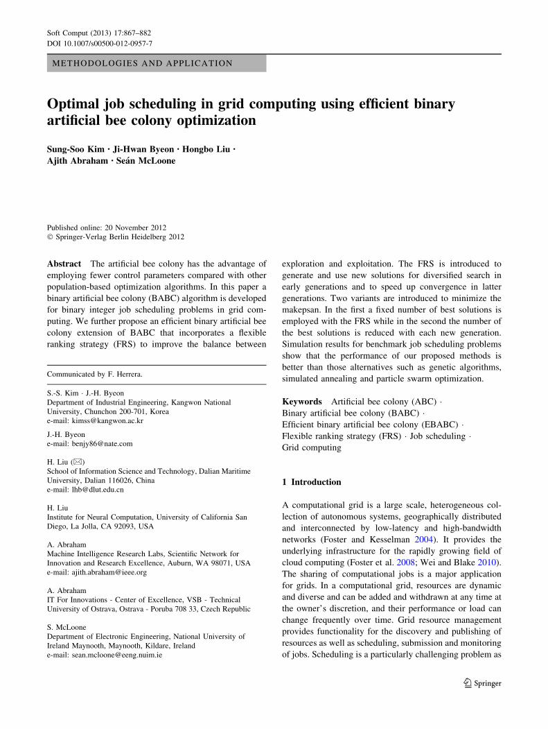
makespan. For example, the jobs J1, J2, J3, J6, J7, J9 and
J12 are allocated on grid node 1 in Fig. 1, C1,1 =
1.5, C1,2 = 3, C1,3 = 4, C1,6 = 7, C1,7 = 7.5, C1,9 = 10
and C1,12 = 13. For grid node 1, the single node flowtimePj=1N C1j = 46. The other two grid node flowtimes are also
46. So the makespan is 46 in the schedule solution.
4 Efficient binary artificial bee colony for job
scheduling
In this section, we introduce the EBABC for solving job
scheduling problems. First, the basic artificial bee colony
(ABC) is summarized. Then the BABC is developed for job
scheduling in grid computing. The efficient BABC algo-
rithm (EBABC) is presented as an extension of BABC
incorporating a flexible ranking strategy to improve per-
formance. We also prove that the proposed algorithm con-
verges with a probability of 1 towards the global optimum.
4.1 Artificial bee colony
The ABC is an algorithm motivated by the intelligent
behaviour exhibited by honeybees when searching for
food. The performance of ABC is better than or similar to
other population-based algorithms with the added advan-
tage of employing fewer control parameters (Ma et al.
2011; Li et al. 2012). The only important control parameter
for ABC is Limit; the number of unsuccessful trials before
a food source is deemed to be abandoned (Karaboga and
Akay 2009; Karaboga and Basturk 2007, 2008). The main
steps of the basic ABC algorithm are summarized in
Algorithm 1 (Karaboga and Akay 2009).
In ABC, the colony of artificial bees contains three
groups of bees: employed bees, onlooker bees and scout
bees. For every food source (FS) there is only one
employed bee. A fitness function is used to assign a quality
or ‘nectar’ value to the food sources. Each employed bee
searches for a new food source within its own neighbour-
hood and moves to it if it has a higher nectar value.
Employed bees then share their food source information
(location and nectar value) with the onlooker bees waiting
in the hive. Each onlooker bee then selects one of the
employed bee food sources probabilistically in a process
similar to roulette wheel selection, The probability
assigned to the kth food source, Pk, is given by
Fig. 1 The scheduling solution
for (3, 13)
870 S.-S. Kim et al.
123
Pk ¼1fkPSNi¼1
1fi
ð4Þ
where fk is the nectar value of the kth food source and SN is the
total number of food sources (=Number of employed bees).
After selecting its food source each onlooker bee then seeks
out one new food source within its neighbourhood and moves
to this food source if it has a higher nectar value. If the number
of active food sources outnumbers the maximum allowed,
those with the lowest nectar values are abandoned. An
employed bee for a food source that has been abandoned
becomes a scout bee and starts to search for a new food source
randomly. Thus, while onlooker bees and employed bees are
targeted at exploitation, scout bees provide a mechanism for
exploration (Karaboga and Basturk 2008).
4.2 Binary artificial bee colony
The BABC algorithm is formulated in this section for appli-
cation to job scheduling in grid computing. A job scheduling
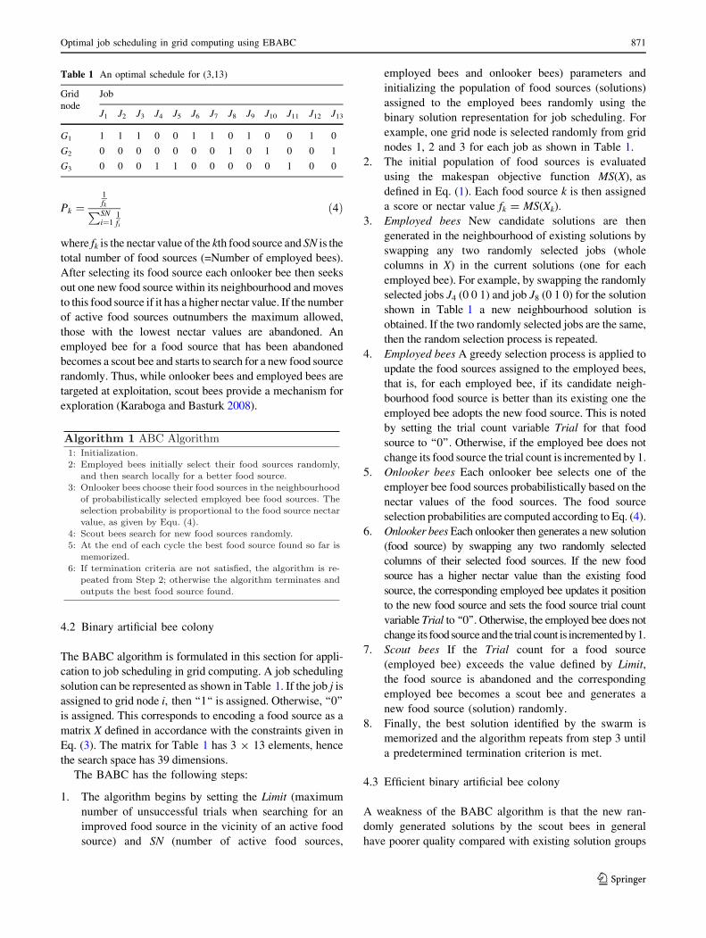
solution can be represented as shown in Table 1. If the job j is
assigned to grid node i, then ‘‘1‘‘ is assigned. Otherwise, ‘‘0’’
is assigned. This corresponds to encoding a food source as a
matrix X defined in accordance with the constraints given in
Eq. (3). The matrix for Table 1 has 3 9 13 elements, hence
the search space has 39 dimensions.
The BABC has the following steps:
1. The algorithm begins by setting the Limit (maximum
number of unsuccessful trials when searching for an
improved food source in the vicinity of an active food
source) and SN (number of active food sources,
employed bees and onlooker bees) parameters and
initializing the population of food sources (solutions)
assigned to the employed bees randomly using the
binary solution representation for job scheduling. For
example, one grid node is selected randomly from grid
nodes 1, 2 and 3 for each job as shown in Table 1.
2. The initial population of food sources is evaluated
using the makespan objective function MS(X), as
defined in Eq. (1). Each food source k is then assigned
a score or nectar value fk = MS(Xk).
3. Employed bees New candidate solutions are then
generated in the neighbourhood of existing solutions by
swapping any two randomly selected jobs (whole
columns in X) in the current solutions (one for each
employed bee). For example, by swapping the randomly
selected jobs J4 (0 0 1) and job J8 (0 1 0) for the solution
shown in Table 1 a new neighbourhood solution is
obtained. If the two randomly selected jobs are the same,
then the random selection process is repeated.
4. Employed bees A greedy selection process is applied to
update the food sources assigned to the employed bees,
that is, for each employed bee, if its candidate neigh-
bourhood food source is better than its existing one the
employed bee adopts the new food source. This is noted
by setting the trial count variable Trial for that food
source to ‘‘0’’. Otherwise, if the employed bee does not
change its food source the trial count is incremented by 1.
5. Onlooker bees Each onlooker bee selects one of the
employer bee food sources probabilistically based on the
nectar values of the food sources. The food source
selection probabilities are computed according to Eq. (4).
6. Onlooker bees Each onlooker then generates a new solution
(food source) by swapping any two randomly selected
columns of their selected food sources. If the new food
source has a higher nectar value than the existing food
source, the corresponding employed bee updates it position
to the new food source and sets the food source trial count
variable Trial to ‘‘0’’. Otherwise, the employed bee does not
change its food source and the trial count is incremented by1.
7. Scout bees If the Trial count for a food source
(employed bee) exceeds the value defined by Limit,
the food source is abandoned and the corresponding
employed bee becomes a scout bee and generates a
new food source (solution) randomly.
8. Finally, the best solution identified by the swarm is
memorized and the algorithm repeats from step 3 until
a predetermined termination criterion is met.
4.3 Efficient binary artificial bee colony
A weakness of the BABC algorithm is that the new ran-
domly generated solutions by the scout bees in general
have poorer quality compared with existing solution groups
Table 1 An optimal schedule for (3,13)
Grid
node
Job
J1 J2 J3 J4 J5 J6 J7 J8 J9 J10 J11 J12 J13
G1 1 1 1 0 0 1 1 0 1 0 0 1 0
G2 0 0 0 0 0 0 0 1 0 1 0 0 1
G3 0 0 0 1 1 0 0 0 0 0 1 0 0
Optimal job scheduling in grid computing using EBABC 871
123
identified by the employee and onlooker bees. Even though
the generation of random solutions is desirable for exploration
purposes the overall performance of the algorithm can be
impacted as the number of these solutions is increased. In
order to solve this problem and to generate new solutions
whose quality is not significantly different from existing
solutions we propose a modification to the BABC algorithm
involving a flexible ranking strategy (FRS). The resulting
algorithm, referred to as the EBABC algorithm, is summa-
rized in Algorithm 2. Steps 1 to 10 of EBABC correspond to
steps 1 to 6 of the BABC algorithm as described in the pre-
vious section. The new FRS step is introduced between step 6
and 7 of the BABC algorithm and proceeds as follows:
– FRS step The food sources of the employed bee popula-
tion are arranged in order of ascending nectar value
(Makespan). Then the worst solution in the population is
removed and a new solution is generated probabilistically
as a combination of the best RSN solutions in the
population. The probability of selecting a job from the kth
solution among the RSN best solutions is computed as
Pk ¼1fkPRSN
i¼11fi
ð5Þ
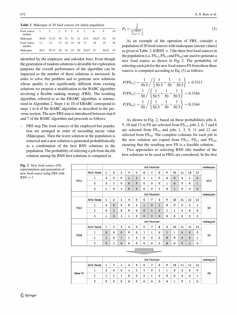
As an example of the operation of FRS, consider a
population of 20 food sources with makespans (nectar values)
as given in Table 2. If RSN = 3 the three best food sources in
the population (i.e. FS11, FS13 and FS16) are used to generate a
new food source as shown in Fig. 2. The probability of
selecting each job for the new food source FS from these three
sources is computed according to Eq. (5) as follows:
PðFS11Þ ¼1
50:5
1
50:5þ 1
50þ 1
50:5
� ��¼ 0:3311
PðFS13Þ ¼1
50
1
50:5þ 1
50þ 1
50:5
� �¼ 0:3344
�
PðFS16Þ ¼1
50
1
50:5þ 1
50þ 1
50:5
� �¼ 0:3344
�
As shown in Fig. 2, based on these probabilities jobs 4,
5, 10 and 13 in FS are selected from FS11, jobs 2, 6, 7 and 8
are selected from FS13 and jobs 1, 3, 9, 11 and 12 are
selected from FS16. The complete columns for each job in
the new solution are copied from FS11, FS13 and FS16,
ensuring that the resulting new FS is a feasible solution.
Two approaches to selecting RSN (the number of the
best solutions to be used in FRS) are considered. In the first
Fig. 2 New food source (FS)
representation and generation of
new food source using FRS with
RSN = 3
Table 2 Makespan of 20 food sources for initial population
Food sourcenumber
1 2 3 4 5 6 7 8 9 10
Makespan 50.67 51.33 54 51 51 51 51.5 50.67 52 54
Food sourcenumber
11 12 13 14 15 16 17 18 19 20
Makespan 50.5 55.33 50 52 55 50 54.67 51 50.67 55
872 S.-S. Kim et al.
123
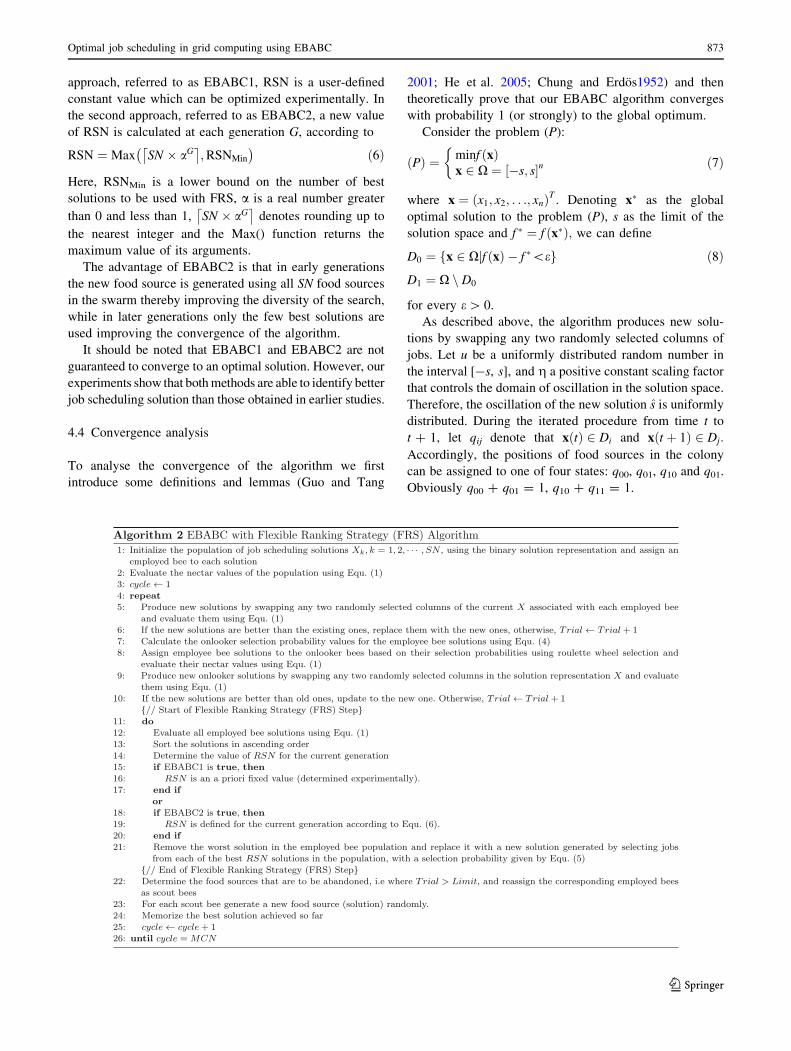
approach, referred to as EBABC1, RSN is a user-defined
constant value which can be optimized experimentally. In
the second approach, referred to as EBABC2, a new value
of RSN is calculated at each generation G, according to
RSN ¼ Max SN � aG� �
;RSNMin
� �ð6Þ
Here, RSNMin is a lower bound on the number of best
solutions to be used with FRS, a is a real number greater
than 0 and less than 1, SN � aG� �
denotes rounding up to
the nearest integer and the Max() function returns the
maximum value of its arguments.
The advantage of EBABC2 is that in early generations
the new food source is generated using all SN food sources
in the swarm thereby improving the diversity of the search,
while in later generations only the few best solutions are
used improving the convergence of the algorithm.
It should be noted that EBABC1 and EBABC2 are not
guaranteed to converge to an optimal solution. However, our
experiments show that both methods are able to identify better
job scheduling solution than those obtained in earlier studies.
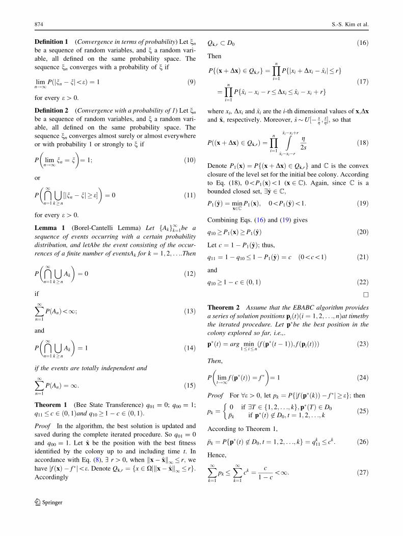
4.4 Convergence analysis
To analyse the convergence of the algorithm we first
introduce some definitions and lemmas (Guo and Tang
2001; He et al. 2005; Chung and Erdos1952) and then
theoretically prove that our EBABC algorithm converges
with probability 1 (or strongly) to the global optimum.
Consider the problem (P):
ðPÞ ¼ minf ðxÞx 2 X ¼ ½�s; s�n
�ð7Þ
where x ¼ ðx1; x2; . . .; xnÞT . Denoting x� as the global
optimal solution to the problem (P), s as the limit of the
solution space and f � ¼ f ðx�Þ; we can define
D0 ¼ fx 2 Xjf ðxÞ � f �\eg ð8ÞD1 ¼ X n D0
for every e [ 0.
As described above, the algorithm produces new solu-
tions by swapping any two randomly selected columns of
jobs. Let u be a uniformly distributed random number in
the interval [-s, s], and g a positive constant scaling factor
that controls the domain of oscillation in the solution space.
Therefore, the oscillation of the new solution s is uniformly
distributed. During the iterated procedure from time t to
t ? 1, let qij denote that xðtÞ 2 Di and xðt þ 1Þ 2 Dj:
Accordingly, the positions of food sources in the colony
can be assigned to one of four states: q00, q01, q10 and q01.
Obviously q00 ? q01 = 1, q10 ? q11 = 1.
Optimal job scheduling in grid computing using EBABC 873
123
Definition 1 (Convergence in terms of probability) Let nn
be a sequence of random variables, and n a random vari-
able, all defined on the same probability space. The
sequence nn converges with a probability of n if
limn!1
Pðjnn � nj\eÞ ¼ 1 ð9Þ
for every e [ 0.
Definition 2 (Convergence with a probability of 1) Let nn
be a sequence of random variables, and n a random vari-
able, all defined on the same probability space. The
sequence nn converges almost surely or almost everywhere
or with probability 1 or strongly to n if
P
lim
n!1nn ¼ n
¼ 1; ð10Þ
or
P
\1
n¼1
[
k� n
½jnn � nj � e�¼ 0 ð11Þ
for every e [ 0.
Lemma 1 (Borel-Cantelli Lemma) Let fAkg1k¼1be a
sequence of events occurring with a certain probability
distribution, and letAbe the event consisting of the occur-
rences of a finite number of eventsAk for k ¼ 1; 2; . . .:Then
P
\1
n¼1
[
k� n
Ak
¼ 0 ð12Þ
if
X1
n¼1
PðAnÞ\1; ð13Þ
and
P
\1
n¼1
[
k� n
Ak
¼ 1 ð14Þ
if the events are totally independent and
X1
n¼1
PðAnÞ ¼ 1: ð15Þ
Theorem 1 (Bee State Transference) q01 = 0; q00 = 1;
q11� c 2 ð0; 1Þand q10� 1� c 2 ð0; 1Þ:
Proof In the algorithm, the best solution is updated and
saved during the complete iterated procedure. So q01 = 0
and q00 = 1. Let x be the position with the best fitness
identified by the colony up to and including time t. In
accordance with Eq. (8), A r [ 0, when kx� xk1 � r; we
have jf ðxÞ � f �j\e: Denote Qx;r ¼ fx 2 Xjkx� xk1 � rg:Accordingly
Qx;r D0 ð16Þ
Then
Pfðxþ DxÞ 2 Qx;rg ¼Yn
i¼1
Pfjxi þ Dxi � xij � rg
¼Yn
i¼1
Pfxi � xi � r�Dxi� xi � xi þ rgð17Þ
where xi, Dxi and xi are the i-th dimensional values of x;Dx
and x; respectively. Moreover, sU½� sg ;
sg�; so that
Pððxþ DxÞ 2 Qx;rÞ ¼Yn
i¼1
Zxi�xiþr
xi�xi�r
g2s
ð18Þ
Denote P1ðxÞ ¼ Pfðxþ DxÞ 2 Qx;rg and C is the convex
closure of the level set for the initial bee colony. According
to Eq. (18), 0\P1ðxÞ\1 (x 2 C). Again, since C is a
bounded closed set, 9y 2 C;
P1ðyÞ ¼ minx2C
P1ðxÞ; 0\P1ðyÞ\1: ð19Þ
Combining Eqs. (16) and (19) gives
q10�P1ðxÞ�P1ðyÞ ð20Þ
Let c ¼ 1� P1ðyÞ; thus,
q11 ¼ 1� q10� 1� P1ðyÞ ¼ c ð0\c\1Þ ð21Þ
and
q10� 1� c 2 ð0; 1Þ ð22Þ
h
Theorem 2 Assume that the EBABC algorithm provides
a series of solution positions piðtÞði ¼ 1; 2; . . .; nÞat timetby
the iterated procedure. Let p�be the best position in the
colony explored so far, i.e.,.
p�ðtÞ ¼ arg min1� i� n
ðf ðp�ðt � 1ÞÞ; f ðpiðtÞÞÞ ð23Þ
Then,
P
limt!1
f ðp�ðtÞÞ ¼ f �¼ 1 ð24Þ
Proof For 8e [ 0; let pk ¼ Pfjf ðp�ðkÞÞ � f �j � eg; then
pk ¼0 if 9T 2 f1; 2; . . .; kg; p�ðTÞ 2 D0
�pk if p�ðtÞ 62 D0; t ¼ 1; 2; . . .; k
�ð25Þ
According to Theorem 1,
�pk ¼ Pfp�ðtÞ 62 D0; t ¼ 1; 2; . . .; kg ¼ qk11� ck: ð26Þ
Hence,
X1
k¼1
pk �X1
k¼1
ck ¼ c
1� c\1: ð27Þ
874 S.-S. Kim et al.
123
According to Lemma 1,
P
\1
t¼1
[
k� t
jf ðp�ðkÞÞ � f �j � e
¼ 0 ð28Þ
Therefore, as defined in Definition 2, the sequence f ðp�ðtÞÞconverges almost surely or almost everywhere or with
probability 1 or strongly towards f*. The theorem is
proven. h
5 Experiments and analysis
5.1 Experimental settings
In the following sections we present experimental results
for the BABC, EBABC1 and EBABC2 algorithms applied
to a serious of benchmark job scheduling problems as defined
in Liu et al. (2010). The experiments were conducted on a
desktop computer with an IntelrCoreTM2 Duo 2.66GHz CPU
and 2G RAM. In total seven different dimensions of job
scheduling problem were investigated, namely (3, 13), (5,
100), (8, 60), (10, 50), (10, 100), (60, 500) and (100, 1000).
Here the notation (G, J) is employed to indicate the number of
computing nodes on the grid (G) and number of jobs (J) to be
scheduled for each problem. The specific parameter settings
employed with BABC, EBABC1 and EBABC2 for each
problem are given in Table 3.
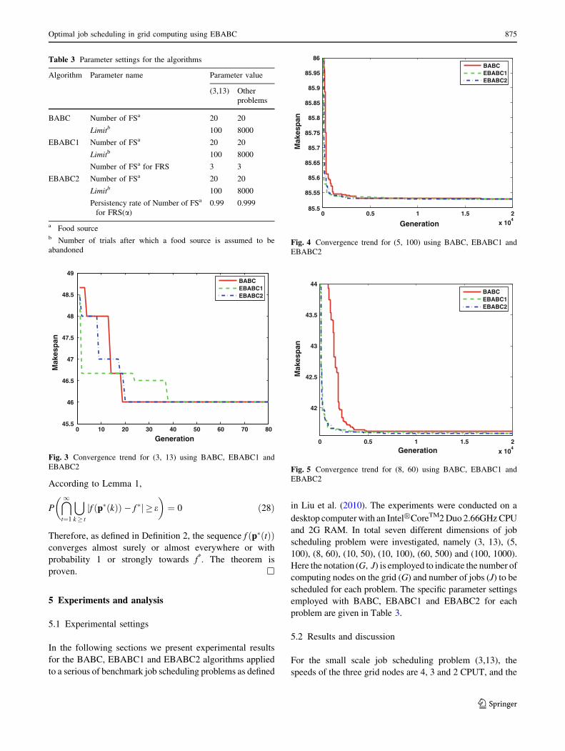
5.2 Results and discussion
For the small scale job scheduling problem (3,13), the
speeds of the three grid nodes are 4, 3 and 2 CPUT, and the
Table 3 Parameter settings for the algorithms
Algorithm Parameter name Parameter value
(3,13) Other
problems
BABC Number of FSa 20 20
Limitb 100 8000
EBABC1 Number of FSa 20 20
Limitb 100 8000
Number of FSa for FRS 3 3
EBABC2 Number of FSa 20 20
Limitb 100 8000
Persistency rate of Number of FSa
for FRS(a)
0.99 0.999
a Food sourceb Number of trials after which a food source is assumed to be
abandoned
0 0.5 1 1.5 2
x 104
42
42.5
43
43.5
44
Generation
Mak
esp
anBABCEBABC1EBABC2
Fig. 5 Convergence trend for (8, 60) using BABC, EBABC1 and
EBABC2
0 0.5 1 1.5 2
x 104
85.5
85.55
85.6
85.65
85.7
85.75
85.8
85.85
85.9
85.95
86
Generation
Mak
esp
an
BABCEBABC1EBABC2
Fig. 4 Convergence trend for (5, 100) using BABC, EBABC1 and
EBABC2
0 10 20 30 40 50 60 70 8045.5
46
46.5
47
47.5
48
48.5
49
Generation
Mak
esp
an
BABCEBABC1EBABC2
Fig. 3 Convergence trend for (3, 13) using BABC, EBABC1 and
EBABC2
Optimal job scheduling in grid computing using EBABC 875
123
job lengths of the 13 jobs are 6, 12, 16, 20, 24, 28, 30, 36,
40, 42, 48, 52 and 60 cycles. Figure 3 shows the conver-
gence trend for job scheduling (3, 13) using BABC,
EBABC1 and EBABC2. In the best job scheduling solution
jobs 1, 2, 3, 6, 7, 9 and 12 are assigned to grid node 1, jobs
8, 10 and 13 are assigned to grid node 2 and the jobs 4, 5
and 11 are assigned to node 3 as shown in Fig. 1. The
optimal makespan is 46. This is computed by dividing the
total job length on each grid node by its speed and selecting
the largest value. Thus, grid node 1 gives (6 ? 12 ?
16 ? 28 ? 30 ? 40 ? 52)/4 = 46, grid node 2 gives
(36 ? 42 ? 60)/3=46 and grid node 3 gives (20 ? 24 ?
48)/2 = 46. Since all grid nodes have identical computation
times this is the global optimum solution. All ten algorithm
runs of BABC, EBABC1 and EBABC2 identify optimum
solutions (makespan = 46) within 1000 generations. This
compares to success rates of 2, 3 and 4 out of 10 runs
within 2000 generations when using GA, SA and PSO as
reported in Liu et al. (2010).
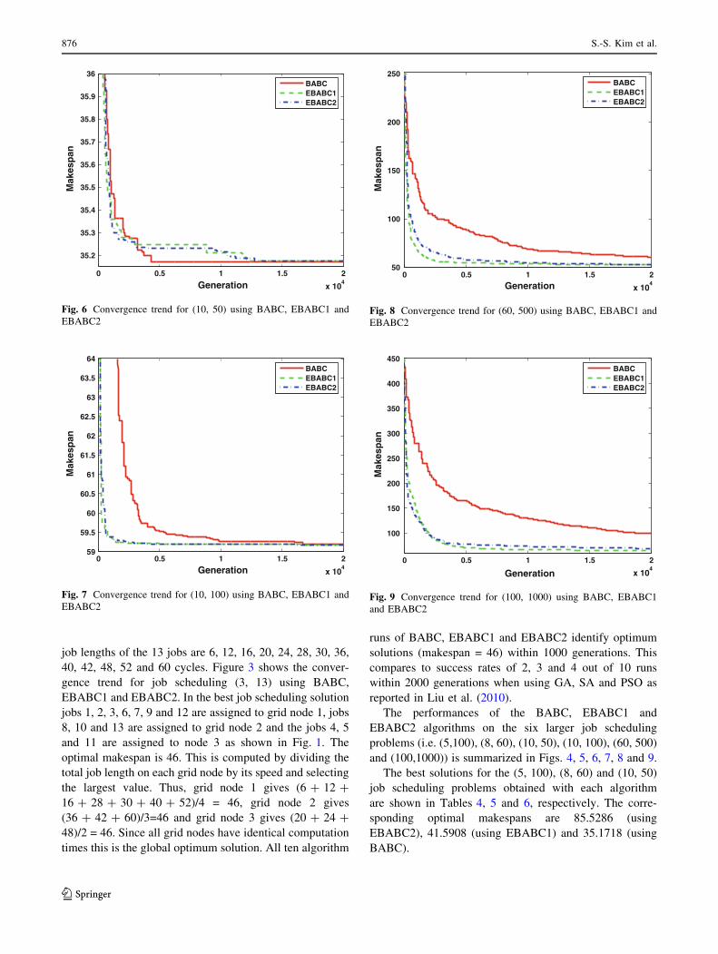
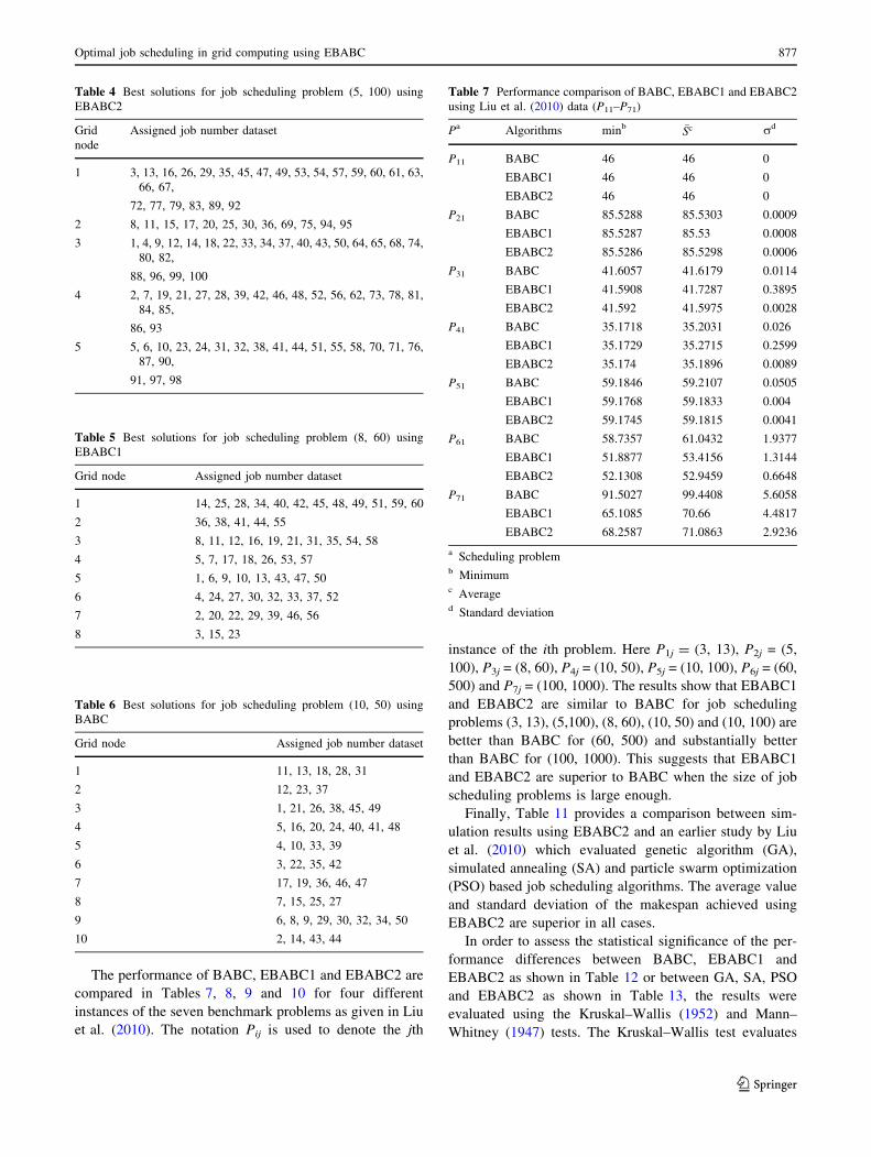
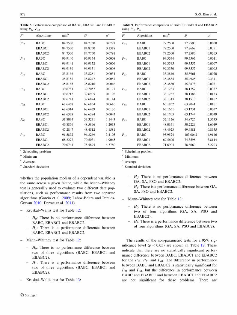
The performances of the BABC, EBABC1 and
EBABC2 algorithms on the six larger job scheduling
problems (i.e. (5,100), (8, 60), (10, 50), (10, 100), (60, 500)
and (100,1000)) is summarized in Figs. 4, 5, 6, 7, 8 and 9.
The best solutions for the (5, 100), (8, 60) and (10, 50)
job scheduling problems obtained with each algorithm
are shown in Tables 4, 5 and 6, respectively. The corre-
sponding optimal makespans are 85.5286 (using
EBABC2), 41.5908 (using EBABC1) and 35.1718 (using
BABC).
0 0.5 1 1.5 2
x 104
100
150
200
250
300
350
400
450
Generation
Mak
esp
anBABCEBABC1EBABC2
Fig. 9 Convergence trend for (100, 1000) using BABC, EBABC1
and EBABC2
0 0.5 1 1.5 2
x 104
50
100
150
200
250
Generation
Mak
esp
an
BABCEBABC1EBABC2
Fig. 8 Convergence trend for (60, 500) using BABC, EBABC1 and
EBABC2
0 0.5 1 1.5 2
x 104
59
59.5
60
60.5
61
61.5
62
62.5
63
63.5
64
Generation
Mak
esp
an
BABCEBABC1EBABC2
Fig. 7 Convergence trend for (10, 100) using BABC, EBABC1 and
EBABC2
0 0.5 1 1.5 2
x 104
35.2
35.3
35.4
35.5
35.6
35.7
35.8
35.9
36
Generation
Mak
esp
an
BABCEBABC1EBABC2
Fig. 6 Convergence trend for (10, 50) using BABC, EBABC1 and
EBABC2
876 S.-S. Kim et al.
123
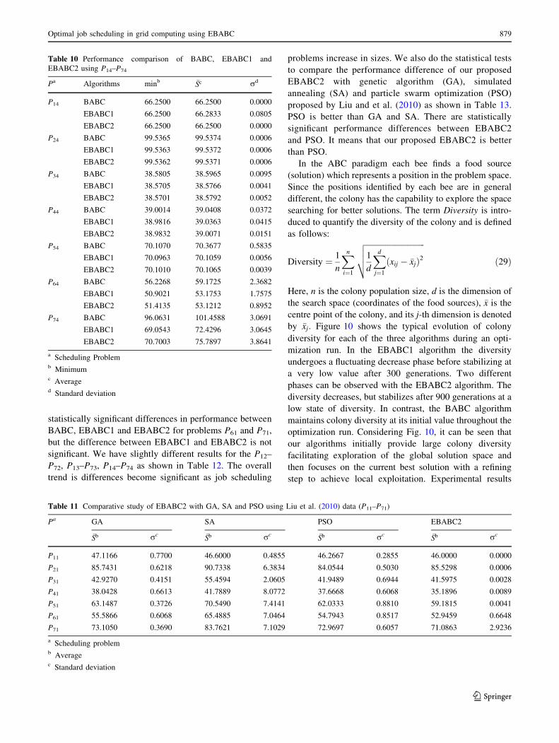
The performance of BABC, EBABC1 and EBABC2 are
compared in Tables 7, 8, 9 and 10 for four different
instances of the seven benchmark problems as given in Liu
et al. (2010). The notation Pij is used to denote the jth
instance of the ith problem. Here P1j = (3, 13), P2j = (5,
100), P3j = (8, 60), P4j = (10, 50), P5j = (10, 100), P6j = (60,
500) and P7j = (100, 1000). The results show that EBABC1
and EBABC2 are similar to BABC for job scheduling
problems (3, 13), (5,100), (8, 60), (10, 50) and (10, 100) are
better than BABC for (60, 500) and substantially better
than BABC for (100, 1000). This suggests that EBABC1
and EBABC2 are superior to BABC when the size of job
scheduling problems is large enough.
Finally, Table 11 provides a comparison between sim-
ulation results using EBABC2 and an earlier study by Liu
et al. (2010) which evaluated genetic algorithm (GA),
simulated annealing (SA) and particle swarm optimization
(PSO) based job scheduling algorithms. The average value
and standard deviation of the makespan achieved using
EBABC2 are superior in all cases.
In order to assess the statistical significance of the per-
formance differences between BABC, EBABC1 and
EBABC2 as shown in Table 12 or between GA, SA, PSO
and EBABC2 as shown in Table 13, the results were
evaluated using the Kruskal–Wallis (1952) and Mann–
Whitney (1947) tests. The Kruskal–Wallis test evaluates
Table 6 Best solutions for job scheduling problem (10, 50) using
BABC
Grid node Assigned job number dataset
1 11, 13, 18, 28, 31
2 12, 23, 37
3 1, 21, 26, 38, 45, 49
4 5, 16, 20, 24, 40, 41, 48
5 4, 10, 33, 39
6 3, 22, 35, 42
7 17, 19, 36, 46, 47
8 7, 15, 25, 27
9 6, 8, 9, 29, 30, 32, 34, 50
10 2, 14, 43, 44
Table 4 Best solutions for job scheduling problem (5, 100) using
EBABC2
Grid
node
Assigned job number dataset
1 3, 13, 16, 26, 29, 35, 45, 47, 49, 53, 54, 57, 59, 60, 61, 63,
66, 67,
72, 77, 79, 83, 89, 92
2 8, 11, 15, 17, 20, 25, 30, 36, 69, 75, 94, 95
3 1, 4, 9, 12, 14, 18, 22, 33, 34, 37, 40, 43, 50, 64, 65, 68, 74,
80, 82,
88, 96, 99, 100
4 2, 7, 19, 21, 27, 28, 39, 42, 46, 48, 52, 56, 62, 73, 78, 81,
84, 85,
86, 93
5 5, 6, 10, 23, 24, 31, 32, 38, 41, 44, 51, 55, 58, 70, 71, 76,
87, 90,
91, 97, 98
Table 5 Best solutions for job scheduling problem (8, 60) using
EBABC1
Grid node Assigned job number dataset
1 14, 25, 28, 34, 40, 42, 45, 48, 49, 51, 59, 60
2 36, 38, 41, 44, 55
3 8, 11, 12, 16, 19, 21, 31, 35, 54, 58
4 5, 7, 17, 18, 26, 53, 57
5 1, 6, 9, 10, 13, 43, 47, 50
6 4, 24, 27, 30, 32, 33, 37, 52
7 2, 20, 22, 29, 39, 46, 56
8 3, 15, 23
Table 7 Performance comparison of BABC, EBABC1 and EBABC2
using Liu et al. (2010) data (P11–P71)
Pa Algorithms minb �Sc rd
P11 BABC 46 46 0
EBABC1 46 46 0
EBABC2 46 46 0
P21 BABC 85.5288 85.5303 0.0009
EBABC1 85.5287 85.53 0.0008
EBABC2 85.5286 85.5298 0.0006
P31 BABC 41.6057 41.6179 0.0114
EBABC1 41.5908 41.7287 0.3895
EBABC2 41.592 41.5975 0.0028
P41 BABC 35.1718 35.2031 0.026
EBABC1 35.1729 35.2715 0.2599
EBABC2 35.174 35.1896 0.0089
P51 BABC 59.1846 59.2107 0.0505
EBABC1 59.1768 59.1833 0.004
EBABC2 59.1745 59.1815 0.0041
P61 BABC 58.7357 61.0432 1.9377
EBABC1 51.8877 53.4156 1.3144
EBABC2 52.1308 52.9459 0.6648
P71 BABC 91.5027 99.4408 5.6058
EBABC1 65.1085 70.66 4.4817
EBABC2 68.2587 71.0863 2.9236
a Scheduling problemb Minimumc Averaged Standard deviation
Optimal job scheduling in grid computing using EBABC 877
123
whether the population median of a dependent variable is
the same across a given factor, while the Mann–Whitney
test is generallly used to evaluate two different data pop-
ulations, such as performance results from two separate
algorithms (Garcıa et al. 2009; Lahoz-Beltra and Perales-
Gravan 2010; Derrac et al. 2011).
– Kruskal–Wallis test for Table 12:
– H0: There is no performance difference between
BABC, EBABC1 and EBABC2.
– H1: There is a performance difference between
BABC, EBABC1 and EBABC2.
– Mann–Whitney test for Table 12:
– H0: There is no performance difference between
two of three algorithms (BABC, EBABC1 and
EBABC2).
– H1: There is a performance difference between
two of three algorithms (BABC, EBABC1 and
EBABC2).
– Kruskal–Wallis test for Table 13:
– H0: There is no performance difference between
GA, SA, PSO and EBABC2.
– H1: There is a performance difference between GA,
SA, PSO and EBABC2.
– Mann–Whitney test for Table 13:
– H0: There is no performance difference between
two of four algorithms (GA, SA, PSO and
EBABC2).
– H1: There is a performance difference between two
of four algorithms (GA, SA, PSO and EBABC2).
The results of the non-parametric tests for a 95% sig-
nificance level (p \ 0.05) are shown in Table 12. These
indicate that there are no statistically significant perfor-
mance difference between BABC, EBABC1 and EBABC2
for the P11, P21 and P41. The difference in performance
between BABC and EBABC2 is statistically significant for
P31 and P51, but the difference in performance between
BABC and EBABC1 and between EBABC1 and EBABC2
are not significant for these problems. There are
Table 8 Performance comparison of BABC, EBABC1 and EBABC2
using P12–P72
Pa Algorithms minb �Sc rd
P12 BABC 84.7500 84.7750 0.0791
EBABC1 84.7500 84.8750 0.1318
EBABC2 84.7500 84.7750 0.0791
P22 BABC 96.9140 96.9154 0.0008
EBABC1 96.9141 96.9152 0.0006
EBABC2 96.9139 96.9151 0.0008
P32 BABC 35.8166 35.8281 0.0054
EBABC1 35.8187 35.8247 0.0052
EBABC2 35.8165 35.8216 0.0046
P42 BABC 39.6781 39.7057 0.0177
EBABC1 39.6712 39.6905 0.0198
EBABC2 39.6741 39.6874 0.0144
P52 BABC 68.6468 68.6854 0.0616
EBABC1 68.6314 68.6439 0.0136
EBABC2 68.6338 68.6384 0.0043
P62 BABC 51.8034 53.3231 1.1443
EBABC1 46.8856 48.5896 1.2013
EBABC2 47.2847 48.4512 1.1581
P72 BABC 91.5892 96.3269 3.4105
EBABC1 68.2272 70.5031 1.9065
EBABC2 70.0744 75.5895 4.3780
a Scheduling problemb Minimumc Averaged Standard deviation
Table 9 Performance comparison of BABC, EBABC1 and EBABC2
using P13–P73
Pa Algorithms minb �Sc rd
P13 BABC 77.2500 77.2500 0.0000
EBABC1 77.2500 77.2667 0.0351
EBABC2 77.2500 77.2583 0.0263
P23 BABC 99.3544 99.3563 0.0011
EBABC1 99.3545 99.3557 0.0007
EBABC2 99.3550 99.3557 0.0005
P33 BABC 35.3846 35.3961 0.0070
EBABC1 35.3834 35.4925 0.3341
EBABC2 35.3830 35.3878 0.0031
P43 BABC 38.1283 38.1757 0.0387
EBABC1 38.1237 38.1388 0.0133
EBABC2 38.1313 38.1510 0.0167
P53 BABC 63.1832 63.2041 0.0161
EBABC1 63.1651 63.1731 0.0057
EBABC2 63.1705 63.1744 0.0039
P63 BABC 52.1126 54.8725 1.5633
EBABC1 48.0351 50.2229 1.6019
EBABC2 48.4923 49.6881 0.8955
P73 BABC 95.9524 103.0042 4.9146
EBABC1 69.5606 74.3598 3.8114
EBABC2 71.6904 78.8660 5.2703
a Scheduling problemb Minimumc Averaged Standard deviation
878 S.-S. Kim et al.
123
statistically significant differences in performance between
BABC, EBABC1 and EBABC2 for problems P61 and P71,
but the difference between EBABC1 and EBABC2 is not
significant. We have slightly different results for the P12–
P72, P13–P73, P14–P74 as shown in Table 12. The overall
trend is differences become significant as job scheduling
problems increase in sizes. We also do the statistical tests
to compare the performance difference of our proposed
EBABC2 with genetic algorithm (GA), simulated
annealing (SA) and particle swarm optimization (PSO)
proposed by Liu and et al. (2010) as shown in Table 13.
PSO is better than GA and SA. There are statistically
significant performance differences between EBABC2
and PSO. It means that our proposed EBABC2 is better
than PSO.
In the ABC paradigm each bee finds a food source
(solution) which represents a position in the problem space.
Since the positions identified by each bee are in general
different, the colony has the capability to explore the space
searching for better solutions. The term Diversity is intro-
duced to quantify the diversity of the colony and is defined
as follows:
Diversity ¼ 1
n
Xn
i¼1
ffiffiffiffiffiffiffiffiffiffiffiffiffiffiffiffiffiffiffiffiffiffiffiffiffiffiffiffiffiffi1
d
Xd
j¼1
ðxij � �xjÞ2vuut ð29Þ
Here, n is the colony population size, d is the dimension of
the search space (coordinates of the food sources), �x is the
centre point of the colony, and its j-th dimension is denoted
by �xj: Figure 10 shows the typical evolution of colony
diversity for each of the three algorithms during an opti-
mization run. In the EBABC1 algorithm the diversity
undergoes a fluctuating decrease phase before stabilizing at
a very low value after 300 generations. Two different
phases can be observed with the EBABC2 algorithm. The
diversity decreases, but stabilizes after 900 generations at a
low state of diversity. In contrast, the BABC algorithm
maintains colony diversity at its initial value throughout the
optimization run. Considering Fig. 10, it can be seen that
our algorithms initially provide large colony diversity
facilitating exploration of the global solution space and
then focuses on the current best solution with a refining
step to achieve local exploitation. Experimental results
Table 10 Performance comparison of BABC, EBABC1 and
EBABC2 using P14–P74
Pa Algorithms minb �Sc rd
P14 BABC 66.2500 66.2500 0.0000
EBABC1 66.2500 66.2833 0.0805
EBABC2 66.2500 66.2500 0.0000
P24 BABC 99.5365 99.5374 0.0006
EBABC1 99.5363 99.5372 0.0006
EBABC2 99.5362 99.5371 0.0006
P34 BABC 38.5805 38.5965 0.0095
EBABC1 38.5705 38.5766 0.0041
EBABC2 38.5701 38.5792 0.0052
P44 BABC 39.0014 39.0408 0.0372
EBABC1 38.9816 39.0363 0.0415
EBABC2 38.9832 39.0071 0.0151
P54 BABC 70.1070 70.3677 0.5835
EBABC1 70.0963 70.1059 0.0056
EBABC2 70.1010 70.1065 0.0039
P64 BABC 56.2268 59.1725 2.3682
EBABC1 50.9021 53.1753 1.7575
EBABC2 51.4135 53.1212 0.8952
P74 BABC 96.0631 101.4588 3.0691
EBABC1 69.0543 72.4296 3.0645
EBABC2 70.7003 75.7897 3.8641
a Scheduling Problemb Minimumc Averaged Standard deviation
Table 11 Comparative study of EBABC2 with GA, SA and PSO using Liu et al. (2010) data (P11–P71)
Pa GA SA PSO EBABC2
�Sb rc �Sb rc �Sb rc �Sb rc
P11 47.1166 0.7700 46.6000 0.4855 46.2667 0.2855 46.0000 0.0000
P21 85.7431 0.6218 90.7338 6.3834 84.0544 0.5030 85.5298 0.0006
P31 42.9270 0.4151 55.4594 2.0605 41.9489 0.6944 41.5975 0.0028
P41 38.0428 0.6613 41.7889 8.0772 37.6668 0.6068 35.1896 0.0089
P51 63.1487 0.3726 70.5490 7.4141 62.0333 0.8810 59.1815 0.0041
P61 55.5866 0.6068 65.4885 7.0464 54.7943 0.8517 52.9459 0.6648
P71 73.1050 0.3690 83.7621 7.1029 72.9697 0.6057 71.0863 2.9236
a Scheduling problemb Averagec Standard deviation
Optimal job scheduling in grid computing using EBABC 879
123
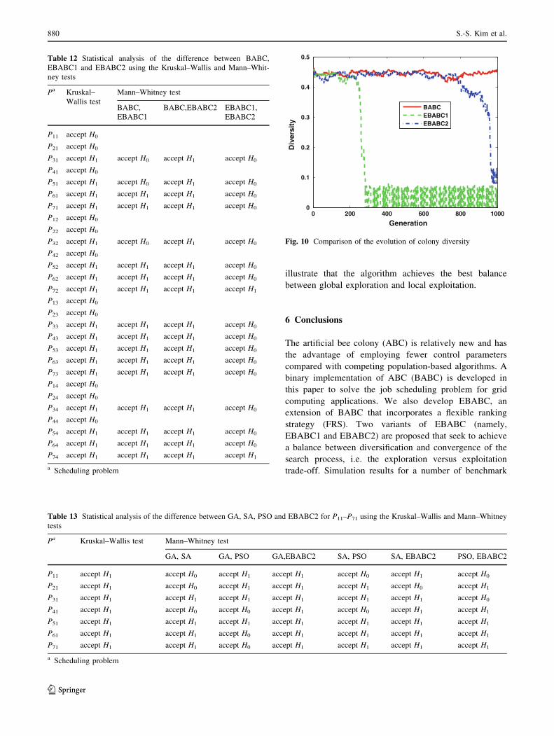
illustrate that the algorithm achieves the best balance
between global exploration and local exploitation.
6 Conclusions
The artificial bee colony (ABC) is relatively new and has
the advantage of employing fewer control parameters
compared with competing population-based algorithms. A
binary implementation of ABC (BABC) is developed in
this paper to solve the job scheduling problem for grid
computing applications. We also develop EBABC, an
extension of BABC that incorporates a flexible ranking
strategy (FRS). Two variants of EBABC (namely,
EBABC1 and EBABC2) are proposed that seek to achieve
a balance between diversification and convergence of the
search process, i.e. the exploration versus exploitation
trade-off. Simulation results for a number of benchmark
Table 12 Statistical analysis of the difference between BABC,
EBABC1 and EBABC2 using the Kruskal–Wallis and Mann–Whit-
ney tests
Pa Kruskal–
Wallis test
Mann–Whitney test
BABC,
EBABC1
BABC,EBABC2 EBABC1,
EBABC2
P11 accept H0
P21 accept H0
P31 accept H1 accept H0 accept H1 accept H0
P41 accept H0
P51 accept H1 accept H0 accept H1 accept H0
P61 accept H1 accept H1 accept H1 accept H0
P71 accept H1 accept H1 accept H1 accept H0
P12 accept H0
P22 accept H0
P32 accept H1 accept H0 accept H1 accept H0
P42 accept H0
P52 accept H1 accept H1 accept H1 accept H0
P62 accept H1 accept H1 accept H1 accept H0
P72 accept H1 accept H1 accept H1 accept H1
P13 accept H0
P23 accept H0
P33 accept H1 accept H1 accept H1 accept H0
P43 accept H1 accept H1 accept H1 accept H0
P53 accept H1 accept H1 accept H1 accept H0
P63 accept H1 accept H1 accept H1 accept H0
P73 accept H1 accept H1 accept H1 accept H0
P14 accept H0
P24 accept H0
P34 accept H1 accept H1 accept H1 accept H0
P44 accept H0
P54 accept H1 accept H1 accept H1 accept H0
P64 accept H1 accept H1 accept H1 accept H0
P74 accept H1 accept H1 accept H1 accept H1
a Scheduling problem
Table 13 Statistical analysis of the difference between GA, SA, PSO and EBABC2 for P11–P71 using the Kruskal–Wallis and Mann–Whitney
tests
Pa Kruskal–Wallis test Mann–Whitney test
GA, SA GA, PSO GA,EBABC2 SA, PSO SA, EBABC2 PSO, EBABC2
P11 accept H1 accept H0 accept H1 accept H1 accept H0 accept H1 accept H0
P21 accept H1 accept H0 accept H1 accept H1 accept H1 accept H0 accept H1
P31 accept H1 accept H1 accept H1 accept H1 accept H1 accept H1 accept H0
P41 accept H1 accept H0 accept H0 accept H1 accept H0 accept H1 accept H1
P51 accept H1 accept H1 accept H1 accept H1 accept H1 accept H1 accept H1
P61 accept H1 accept H1 accept H0 accept H1 accept H1 accept H1 accept H1
P71 accept H1 accept H1 accept H0 accept H1 accept H1 accept H1 accept H1
a Scheduling problem
0 200 400 600 800 10000
0.1
0.2
0.3
0.4
0.5
Generation
Div
ersi
ty
BABCEBABC1EBABC2
Fig. 10 Comparison of the evolution of colony diversity
880 S.-S. Kim et al.
123
job scheduling problems show that EBABC1 and EBABC2
outperform BABC for larger job scheduling problems and
that in general they provide superior results to competing
genetic algorithm, simulated annealing and particle swarm
optimization based job scheduling algorithms.
An analysis of the dynamical diversity of the bee col-
onies further illustrates that the proposed algorithms, and in
particular EBABC2, delivers a good balance between
global exploration and local exploitation.
Acknowledgments The authors would like to thank Zhihua Cui for
his scientific collaboration in this research work. This work is sup-
ported partly by the Kangwon National University, the National
Natural Science Foundation of China (Grant No. 61173035,
61105117), the Fundamental Research Funds for the Central Uni-
versities (Grant No. 2012TD027), the Program for New Century
Excellent Talents in University (Grant No. NCET-11-0861), and the
Dalian Science and Technology Fund (Grant No. 2010J21DW006).
References
Abraham A, Buyya R, Nath B (2000) Nature’s heuristics for
scheduling jobs on computational grids. In: The 8th IEEE
international conference on advanced computing and communi-
cations (ADCOM 2000), pp 45–52
Abraham A, Liu H, Zhao M (2008) Particle swarm scheduling for
work-flow applications in distributed computing environments.
Metaheuristics for scheduling in industrial and manufacturing
applications. Stud Comput Intell 128:327–342
Abraham A, Jatoth R, Rajasekhar A (2012) Hybrid differential
artificial bee colony algorithm. J Comput Theor Nanosci
9(2):249–257
Alzaqebah M, Abdullah S (2011) Comparison on the selection
strategies in the artificial bee colony algorithm for examination
timetabling problems. Int J Soft Comput Eng 1:158–163
Banks A, Vincent J, Phalp K (2009) Natural strategies for search. Nat
Comput 8(3):547–570
Bao L, Zeng J (2009) Comparison and analysis of the selection
mechanism in the artificial bee colony algorithm. In: Ninth
international conference on hybrid intelligent systems, 2009,
HIS’09, vol 1. IEEE, pp 411–416
Bonabeau E, Dorigo M, Theraulaz G (1999) Swarm intelligence: from
natural to artificial systems. Oxford University Press, Oxford
Braun T, Siegel H, Beck N, Boloni L, Maheswaran M, Reuther A,
Robertson J, Theys M, Yao B (2001) A comparison of eleven
static heuristics for mapping a class of independent tasks onto
heterogeneous distributed computing systems. J Parallel Distrib
Comput 61(6):810–837
Brucker P (2007) Scheduling algorithms. Springer, Berlin
Brucker P, Schlie R (1990) Job-shop scheduling with multi-purpose
machines. Comput Lett 45(4):369–375
Chandrasekaran K, Hemamalini S, Simon S, Padhy N (2012) Thermal
unit commitment using binary/real coded artificial bee colony
algorithm. Electric Power Syst Res 84(1):109–119
Chung K, Erdos P (1952) On the application of the Borel-Cantelli
lemma. Trans Am Math Soc 72:179–186
Chung W, Chang R (2009) A new mechanism for resource monitoring in
grid computing. Future Gen Comput Syst 25(1):1–7
Clerc M (2006) Particle swarm optimization. Wiley-ISTE
Cuevas E, Sencion-Echauri F, Zaldivar D, Perez-Cisneros M (2012)
Multi-circle detection on images using artificial bee colony (abc)
optimization. Soft Comput 16(2):1–16
Davidovic T, Selmic M, Teodorovic D (2009) Scheduling indepen-
dent tasks: bee colony optimization approach. In: 17th Mediter-
ranean conference on control and automation, 2009, MED’09.
IEEE, pp 1020–1025
Davis R, Burns A (2011) A survey of hard real-time scheduling for
multiprocessor systems. ACM Comput Surveys 43(4):35
Derrac J, Garcıa S, Molina D, Herrera F (2011) A practical tutorial on
the use of nonparametric statistical tests as a methodology for
comparing evolutionary and swarm intelligence algorithms.
Swarm Evol Comput 1:3–18
Di Martino V, Mililotti M (2004) Sub optimal scheduling in a grid
using genetic algorithms. Parallel Comput 30(5-6):553–565
Dong F Akl S (2006) Scheduling algorithms for grid computing: state
of the art and open problems. Technical report, School of
Computing, Queen’s University, Kingston, Ontario
Forestiero A, Mastroianni C, Spezzano G (2008) So-grid: a self-
organizing grid featuring bio-inspired algorithms. ACM Trans
Auton Adapt Syst 3(2):1–37
Foster I, Kesselman C (2004) The grid: blueprint for a new computing
infrastructure. Morgan Kaufmann
Foster I, Zhao Y, Raicu I, Lu S (2008) Cloud computing and grid
computing 360-degree compared. In: Grid computing environ-
ments workshop, 2008, GCE’08. IEEE, pp 1–10
Fujita S, Yamashita M (2000) Approximation algorithms for multi-
processor scheduling problem. IEICE Trans Inf Syst 83(3):
503–509
Gao Y, Rong H, Huang J (2005) Adaptive grid job scheduling with
genetic algorithms. Future Gen Comput Syst 21(1):151–161
Garcıa S, Molina D, Lozano M, Herrera F (2009) A study on the use
of non-parametric tests for analyzing the evolutionary algorithms
behaviour: a case study on the cecn2005 special session on real
parameter optimization. J Heuristics 15(6):617–644
Garey M, Johnson D (1979) Computers and intractability: a guide to
the theory of NP-completeness. WH Freeman & Co
Guo C, Tang H (2001) Global convergence properties of evolution
stragtegies. Math Numer Sin 23(1):105–110
Han L, Berry D (2008) Semantic-supported and agent-based decen-
tralized grid resource discovery. Future Gen Comput Syst
24(8):806–812
He R, Wang Y, Wang Q, Zhou J, Hu C (2005) Improved particle
swarm optimization based on self-adaptive escape velocity. Chin
J Softw 16(12):2036–2044
Hou E, Ansari N, Ren H (1994) A genetic algorithm for multipro-
cessor scheduling. IEEE Trans Parallel Distrib Syst
5(2):113–120
Izakian H, Ladani B, Abraham A, Snasel V (2010) A discrete particle
swarm optimization approach for grid job scheduling. Int J Innov
Comput Inf Control 6:1–15
Jansen K, Mastrolilli M, Solis-Oba R (2000) Approximation
algorithms for flexible job shop problems. In: Lecture notes in
computer science. LATIN 2000: theoretical informatics, vol
1776, pp 68–77
Karaboga D, Akay B (2009) A comparative study of artificial bee
colony algorithm. Appl Math Comput 214(1):108–132
Karaboga D, Basturk B (2007) A powerful and efficient algorithm for
numerical function optimization: artificial bee colony (abc)
algorithm. J Global Optim 39(3):459–471
Karaboga D, Basturk B (2008) On the performance of artificial bee
colony (abc) algorithm. Appl Soft Comput 8(1):687–697
Kennedy J, Eberhart R, Shi Y (2001) Swarm intelligence. Springer,
Germany
Kruskal W, Wallis W (1952) Use of ranks in one-criterion variance
analysis. J Am Stat Assoc 47:583–621
Laalaoui Y, Drias H (2010) Aco approach with learning for
preemptive scheduling of real-time tasks. Int J Bio-Inspired
Comput 2(6):383–394
Optimal job scheduling in grid computing using EBABC 881
123
Lahoz-Beltra R, Perales-Gravan C (2010) A survey of nonparametric
tests for the statistical analysis of evolutionary computational
experiments. Int J Inf Theor Appl 17(1):41–61
Lee W, Cai W (2011) A novel artificial bee colony algorithm with
diversity strategy. In: 2011 Seventh international conference on
natural computation (ICNC), vol 3. IEEE, pp 1441–1444
Li J, Pan Q, Xie S, Wang S (2011) A hybrid artificial bee colony
algorithm for flexible job shop scheduling problems. Int J
Comput Commun Control 6(2):286–296
Li G, Niu P, Xiao X (2012) Development and investigation of
efficient artificial bee colony algorithm for numerical function
optimization. Appl Soft Comput 12(1):320–332
Liu H, Abraham A, Clerc M (2007) Chaotic dynamic characteristics
in swarm intelligence. Appl Soft Comput 7(3):1019–1026
Liu H, Abraham A, Wang Z (2009) A multi-swarm approach to multi-
objective flexible job-shop scheduling problems. Fundam Inf
95(4):465–489
Liu H, Abraham A, Hassanien A (2010) Scheduling jobs on
computational grids using a fuzzy particle swarm optimization
algorithm. Future Gen Comput Syst 26(8):1336–1343
Ma M, Liang J, Guo M, Fan Y, Yin Y (2011) Sar image segmentation
based on artificial bee colony algorithm. Appl Soft Comput
11(8):5205–5214
Mann H, Whitney D (1947) On a test of whether one of two random
variables is stochastically larger than the other. Ann Math Stat
18(1):50–60
Mastrolilli M, Gambardella L (1999) Effective neighborhood func-
tions for the flexible job shop problem. J Sched 3(1):3–20
Mezura-Montes E, Velez-Koeppel R (2010) Elitist artificial bee colony
for constrained real-parameter optimization. In: 2010 IEEE Con-
gress on evolutionary computation (CEC). IEEE, pp 1–8
Nemeth Z, Sunderam V (2003) Characterizing grids: attributes,
definitions, and formalisms. J Grid Comput 1(1):9–23
Pampara G, Engelbrecht A (2011) Binary artificial bee colony
optimization. In: Proceedings of 2011 IEEE symposium on
swarm intelligence (SIS). IEEE, pp 1–8
Pan Q, Fatih Tasgetiren M, Suganthan P, Chua T (2011) A discrete
artificial bee colony algorithm for the lot-streaming flow shop
scheduling problem. Inf Sci 181(12):2455–2468
Pinedo M (2012) Scheduling: theory, algorithms, and systems.
Springer, Berlin
Ritchie G, Levine J (2003) A fast, effective local search for
scheduling independent jobs in heterogeneous computing
environments. Technical report, Centre for Intelligent Systems
and their Applications, University of Edinburgh
Ritchie G, Levine J (2004) A hybrid ant algorithm for scheduling
independent jobs in heterogeneous computing environments. In:
Proceedings of 23rd workshop of the UK Planning and
Scheduling Special Interest Group, PLANSIG 2004
Sharma T, Pant M (2011) Enhancing the food locations in an artificial
bee colony algorithm. In: 2011 IEEE symposium on swarm
intelligence (SIS). IEEE, pp 1–5
Singh A, Sundar S (2011) An artificial bee colony algorithm for the
minimum routing cost spanning tree problem. Soft Comput
15(12):1–11
Su M, Su S, Zhao Y (2009) A swarm-inspired projection algorithm.
Pattern Recogn Lett 42(11):2764–2786
Thesen A (1998) Design and evaluation of tabu search algorithms for
multiprocessor scheduling. J Heuristics 4(2):141–160
Vivekanandan K, Ramyachitra D, Anbu B (2011) Artificial bee
colony algorithm for grid scheduling. J Converg Inf Technol
6:328–339
Walker R (2007) Purposive behavior of honeybees as the basis of an
experimental search engine. Soft Comput 11(8):697–716
Wei Y, Blake M (2010) Service-oriented computing and cloud
computing: challenges and opportunities. IEEE Internet Comput
14(6):72–75
Wong L, Puan C, Low M, Wong Y (2010) Bee colony optimisation
algorithm with big valley landscape exploitation for job shop
scheduling problems. Int J Bio-Inspired Comput 2(2):85–99
Wu A, Yu H, Jin S, Lin K, Schiavone G (2004) An incremental
genetic algorithm approach to multiprocessor scheduling. IEEE
Trans Parallel Distrib Syst 15(9):824–834
Xhafa F, Carretero J, Abraham A (2007) Genetic algorithm based
schedulers for grid computing systems. Int J Innov Comput Inf
Control 3(5):1–19
Xiao R, Chen W, Chen T (2012) Modeling of ant colony’s labor
division for the multi-project scheduling problem and its solution
by pso. J Comput Theor Nanosci 9(2):223–232
Yang X (2011) Nature-inspired metaheuristic algorithms. Luniver
Press
Yue B, Liu H, Abraham A (2012) Dynamic trajectory and conver-
gence analysis of swarm algorithm. Comput Inf 31(2):371–392
Ziarati K, Akbari R, Zeighami V (2011) On the performance of bee
algorithms for resource-constrained project scheduling problem.
Appl Soft Comput 11:3720–3733
882 S.-S. Kim et al.
123
Recommended