Calhoun: The NPS Institutional Archive
Theses and Dissertations Thesis Collection
1995-09
Optimal loadout of the supply class (AOE 6) fast
combat stores ship
Schmitt, William Joseph
Monterey, California. Naval Postgraduate School
http://hdl.handle.net/10945/35193
NAVAL POSTGRADUATE SCHOOL MONTEREY, CALIFORNIA
THESIS
OPTIMAL LOADOUT OF THE SUPPLY CLASS (AOE 6) FAST COMBAT
STORES SHIP
19960215 015 by
William Joseph Schmitt
September, 1995
Thesis Advisor: William Kroshl
Approved for public release; distribution is unlimited.
DTIC QUALITY INSPECTED 3
REPORT DOCUMENTATION PAGE Form Approved OMB No. 0704-0188
Public reporting burden for this collection of information is estimated to average 1 hour per response, including the time for reviewing instruction, searching existing data sources, gathering and maintaining the data needed, and completing and reviewing the collection of information. Send comments regarding this burden estimate or any other aspect of this collection of information, including suggestions for reducing this burden, to Washington Headquarters Services, Directorate for Information Operations and Reports, 1215 Jefferson Davis Highway, Suite 1204, Arlington, VA 22202-4302, and to the Office of Management and Budget, Paperwork Reduction Project (0704-0188) Washington DC 20503.
1. AGENCY USE ONLY (Leave blank) 2. REPORT DATE September 1995
3. REPORT TYPE AND DATES COVERED Master's Thesis
4. TITLE AND SUBTITLE OPTIMAL LOADOUT OF THE SUPPLY CLASS (APE 6) FAST COMBAT STORES SHIP
6. AUTHOR(S) Schmitt, William Joseph
5. FUNDING NUMBERS
7. PERFORMING ORGANIZATION NAME(S) AND ADDRESS(ES) Naval Postgraduate School Monterey CA 93943-5000
PERFORMING ORGANIZATION REPORT NUMBER
9. SPONSORING/MONITORING AGENCY NAME(S) AND ADDRESS(ES) 10. SPONSORING/MONITORING AGENCY REPORT NUMBER
11. SUPPLEMENTARY NOTES The views expressed in this thesis are those of the author and do not reflect the official policy or position of the Department of Defense or the U.S. Government.
12a. DISTRmUTION/AVAJLABJLITY STATEMENT Approved for public release; distribution is unlimited.
12b. DISTRIBUTION CODE
13. ABSTRACT (maximum 200 words) This analysis develops a methodology to determine the optimal loadout for the Supply (AOE-6) class fast combat stores ship. The methodology employed tests the ability of a Supply class AOE station ship to resupply and rearm a battle group for offensive operations, including combat. Given a generic scenario, the AOE-6 is loaded with ordnance that provides the maximum benefit to the battle group. Once the AOE-6 is loaded with ordnance, several generic battle groups are developed where the quantity of each necessary commodity in the battle group is tracked daily, and the consolidation schedule for the AOE-6 is determined. From this data, the optimization model finds the minimum number of CONSOLS required to maintain the minimum levels and consequently the optimal cargo fuel mix to configure the AOE-6 station ship. The output for each battle group composition is then analyzed and a cargo fuel mix for the AOE-6 is determined that will respond to the largest number of possible tasking with minimum reconfiguration of fuel tanks.
14. SUBJECT TERMS Combat Logistics Force, Underway Replenishment, AOE-6
Supply Class Fast Combat Stores Ship, Station Ship, Logistics, Optimization, Integer Programming, GAMS.
17. SECURITY CLASSIFI- CATION OF REPORT Unclassified
18. SECURITY CLASSIFI- CATION OF THIS PAGE Unclassified
19. SECURITY CLASSIFICA- TION OF ABSTRACT Unclassified
15. NUMBER OF PAGES 175
16. PRICE CODE
20. LIMITATION OF ABSTRACT UL
NSN 7540-01-280-5500 Standard Form 298 (Rev. 2-89) Prescribed by ANSI Std. 239-18 298-102
11
Approved for public release; distribution is unlimited.
OPTIMAL LOADOUT OF THE SUPPLY CLASS (AOE 6)
FAST COMBAT STORES SHIP
William Joseph Schmitt Lieutenant, United States Navy
B.S., U.S. Naval Academy, 1988 Submitted in partial fulfillment
of the requirements for the degree of
MASTER OF SCIENCE IN OPERATIONS RESEARCH
from the
NAVAL POSTGRADUATE SCHOOL September, 1995
Author:
Approved by:
William Joseph Schmitt
William Kroshl, Thesis Advisor
David A. Schrady, Second Reader
Frank Petho, Chairman Department of Operations Research
in
IV
ABSTRACT
This analysis develops a methodology to determine the
optimal loadout for the Supply (AOE-6) class fast combat
stores ship. The methodology employed tests the ability of a
Supply class AOE station ship to resupply and rearm a battle
group for offensive operations, including combat. Given a
generic scenario, the AOE-6 is loaded with ordnance that
provides the maximum benefit to the battle group. Once the
AOE-6 is loaded with ordnance, several generic battle groups
are developed where the quantity of each necessary commodity
in the battle group is tracked daily, and the consolidation
schedule for the AOE-6 is determined. From this data, the
optimization model finds the minimum number of CONSOLS
required to maintain the minimum levels and consequently the
optimal cargo fuel mix to configure the AOE-6 station ship.
The output for each battle group composition is then analyzed
and a cargo fuel mix for the AOE-6 is determined that will
respond to the largest number of possible tasking with minimum
reconfiguration of fuel tanks.
VI
THESIS DISCLAIMER
The reader is cautioned that computer programs developed in
this research may not have been exercised for all cases of
interest. While effort has been made, within the time available, to
ensure the programs are free of computational and logic errors,
they cannot be considered validated. Any application of these
programs without additional verification is at the risk of the
user.
vn
Vlll
TABLE OF CONTENTS
I . INTRODUCTION 1
A. BACKGROUND 1 1. Development and History of the CLF 2 2 . Role of the AOE in Current CLF Planning 4 3. Role of the AOE-6 Class in Future Operations 4
B . THESIS OBJECTIVES 5 1. Thesis Organization 6 2 . Scope of Study. 6
II . SUPPLY CLASS FAST COMBAT STORES SHIP 9
A. INTRODUCTION 9
B . UNREP CAPABILITIES 11
C . AMMUNITION STORAGE 13 1. Ordnance Stowage Planning Factors 15 2 . Method of Ordnance Storage 16
D . STORES AND PROVISIONS 17
E . CARGO FUEL SYSTEM 17
III. SCENARIO DEVELOPMENT 21
A. GENERAL CONCEPT 21 1. Description of Scenario 21
B . DATA BASE SPECIFICS 23 1. DFM 24 2. JP-5 25 3 . Ordnance 27 4 . Stores 29 5 . Summary of Data 31
C. SCENARIO ASSUMPTIONS 32
IV. SURVEY 33
A. SURVEY METHODOLOGY 35 1. Ordnance 36
B . SURVEY QUESTIONNAIRE STATISTICS 36
IX
C . RAW FREQUENCY DATA 38
D . SCALING OF SURVEY RESULTS 40 1. Interval Scale Construction 40 2. Ten-Step Procedure for Obtaining Scale
Values 41 3 . Scale Values from the Survey Data 42
V. MODEL DEVELOPMENT 45
A. ORDNANCE LOAD MODEL 45 1. Methodology 45 2 . Model Assumptions 46 3 . Description 47 4 . Formulation 52
B . CARGO FUEL MODEL 54 1. Methodology 54 2 . Model Assumptions 56 3 . Description 57 4. Formulation 60
C . GENERAL ALGEBRAIC MODEL SYSTEM 61
VI . SUMMARY OF RESULTS AND CONCLUSIONS 63
A. ORDNANCE LOAD MODEL RESULTS 63
B . CARGO FUEL MODEL RESULTS 66 1. Nuclear Powered CV and Escorts (Scenario 1) 67 2. Conventional Powered CV and Escorts
(Scenario 1A) 68 3. Nuclear Powered CV, Escorts and 3 Ship ARG
(Scenario IB) 68 4. Conventional Powered CV, Escorts and 3 Ship
ARG (Scenario 1C) 69
C. ANALYSIS 69 1. Ordnance Load Model 69 2 . Cargo Fuel Model 70
D . SENSITIVITY ANALYSIS 72 1. Ordnance Load Model 72 2 . Cargo Fuel Model 74
a. Impact of Lowering Minimum Commodity Reserve Levels 74
b. Impact of Having a Smaller Battle Group....75
E. SUBSTITUTING THE AOE-1 CLASS FOR THE AOE-6 CLASS AS THE ASSIGNED BATTLE GROUP STATION SHIP 77 1. Ordnance Load Model 78 2 . Cargo Fuel Model 83
F . CONCLUSIONS 85
G. RECOMMENDATIONS FOR FUTURE STUDY. . 86 1. Ordnance Load Model 86 2 . Cargo Fuel Model „ 87
APPENDIX A. UNREP DEVELOPMENT TIMELINE 89
APPENDIX B. USS SUPPLY UNREP STATIONS 91
APPENDIX C. USS SUPPLY AMMUNITION AND CARGO HOLD LAYOUT .93
APPENDIX D. USS SUPPLY CARGO FUEL TANK AND PUMP ROOM LAYOUT....95
APPENDIX E . SURVEY INSTRUCTIONS 97
APPENDIX F . SURVEY 99
APPENDIX G. SURVEY INFORMATION 103
APPENDIX H. DEMONSTRATION OF OBTAINING SCALE VALUES FROM
SURVEY DATA 105
APPENDIX I. SUPPLY (AOE 6) ORDNANCE LOAD MODEL GAMS PROGRAM AND
RESULTS 117
APPENDIX J. SEATTLE (AOE 3) ORDNANCE LOAD MODEL GAMS PROGRAM AND
RESULTS 131
APPENDIX K. SCENARIO 1 GAMS LINEAR PROGRAM 13 9
APPENDIX L. RESULTS OF CARGO FUEL MODEL PROGRAM 143
LIST OF REFERENCES 147
INITIAL DISTRIBUTION LIST 151
XI
Xll
LIST OF FIGURES
1. Transformed Survey Results 44
xui
XIV
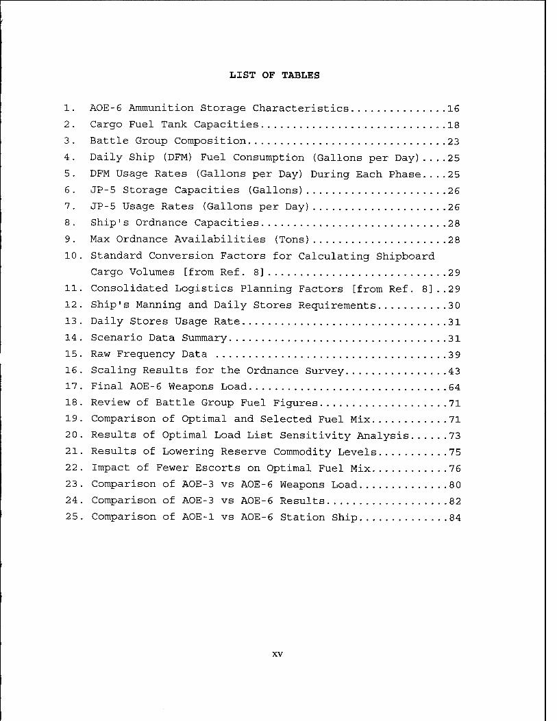
LIST OF TABLES
I. AOE-6 Ammunition Storage Characteristics 16
2 . Cargo Fuel Tank Capacities „ „ . 18
3 . Battle Group Composition 23
4. Daily Ship (DFM) Fuel Consumption (Gallons per Day)....25
5. DFM Usage Rates (Gallons per Day) During Each Phase....25
6. JP-5 Storage Capacities (Gallons) 26
7. JP-5 Usage Rates (Gallons per Day) 26
8 . Ship ' s Ordnance Capacities 28
9. Max Ordnance Availabilities (Tons) 28
10. Standard Conversion Factors for Calculating Shipboard
Cargo Volumes [from Ref. 8] 29
II. Consolidated Logistics Planning Factors [from Ref. 8]..29
12 . Ship' s Manning and Daily Stores Requirements 3 0
13 . Daily Stores Usage Rate 31
14 . Scenario Data Summary 31
15. Raw Frequency Data 3 9
16. Scaling Results for the Ordnance Survey 43
17. Final AOE-6 Weapons Load 64
18 . Review of Battle Group Fuel Figures 71
19. Comparison of Optimal and Selected Fuel Mix 71
20. Results of Optimal Load List Sensitivity Analysis 73
21. Results of Lowering Reserve Commodity Levels 75
22 . Impact of Fewer Escorts on Optimal Fuel Mix 76
23. Comparison of AOE-3 vs AOE-6 Weapons Load 80
24 . Comparison of AOE-3 vs AOE-6 Results 82
25. Comparison of AOE-1 vs AOE-6 Station Ship 84
xv
XVI
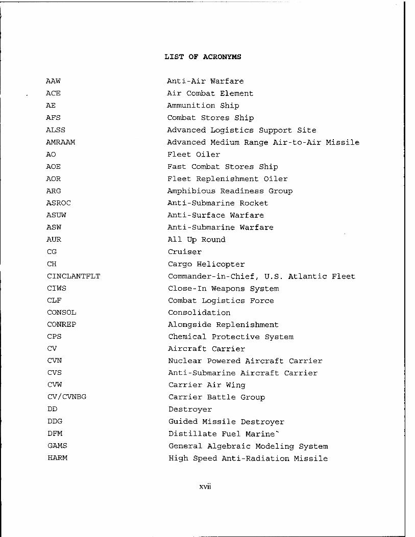
LIST OF ACRONYMS
AAW
ACE
AE
AFS
ALSS
AMRAAM
AO
AOE
AOR
ARG
ASROC
ASUW
ASW
AUR
CG
CH
CINCLANTFLT
CIWS
CLF
CONSOL
CONREP
CPS
CV
CVN
CVS
CVW
CV/CVNBG
DD
DDG
DFM
GAMS
HARM
Anti-Air Warfare
Air Combat Element
Ammunition Ship
Combat Stores Ship
Advanced Logistics Support Site
Advanced Medium Range Air-to-Air Missile
Fleet Oiler
Fast Combat Stores Ship
Fleet Replenishment Oiler
Amphibious Readiness Group
Anti-Submarine Rocket
Anti-Surface Warfare
Anti-Submarine Warfare
All Up Round
Cruiser
Cargo Helicopter
Commander-in-Chief, U.S. Atlantic Fleet
Close-in Weapons System
Combat Logistics Force
Consolidation
Alongside Replenishment
Chemical Protective System
Aircraft Carrier
Nuclear Powered Aircraft Carrier
Anti-Submarine Aircraft Carrier
Carrier Air Wing
Carrier Battle Group
Destroyer
Guided Missile Destroyer
Distillate Fuel Marine"
General Algebraic Modeling System
High Speed Anti-Radiation Missile
xvn
*
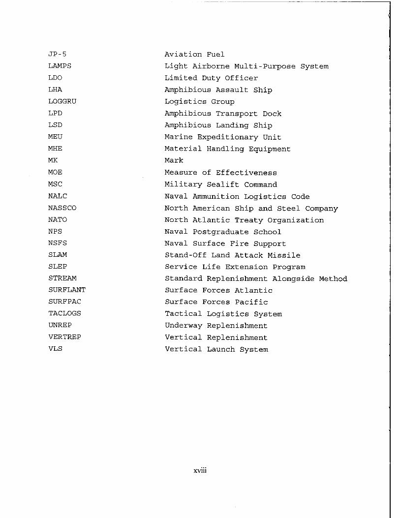
JP-5 Aviation Fuel
LAMPS Light Airborne Multi-Purpose System
LDO Limited Duty Officer
LHA Amphibious Assault Ship
LOGGRU Logistics Group
LPD Amphibious Transport Dock
LSD Amphibious Landing Ship
MEU Marine Expeditionary Unit
MHE Material Handling Equipment
MK Mark
MOE Measure of Effectiveness
MSC Military Sealift Command
NALC Naval Ammunition Logistics Code
NASSCO North American Ship and Steel Company
NATO North Atlantic Treaty Organization
NPS Naval Postgraduate School
NSFS Naval Surface Fire Support
SLAM Stand-Off Land Attack Missile
SLEP Service Life Extension Program
STREAM Standard Replenishment Alongside Method
SURFLANT Surface Forces Atlantic
SURFPAC Surface Forces Pacific
TACLOGS Tactical Logistics System
UNREP Underway Replenishment
VERTREP Vertical Replenishment
VLS Vertical Launch System
xviii
ACKNOWLEDGEMENTS
The author would like to acknowledge the following individuals
for their efforts in making this thesis possible:
Dr. David Morton, for his indispensable help in the design and
testing of the GAMS models.
To the staff at Naval Weapons Station, Earle, especially Mr.
Robert Aten and Ms. Diane Hien, for the time, energy and patience
to teach Ammunition Loading 101.
To CDR William Schworer, MSCLANT N-4, for allowing me to get
such a fast start on this project. Your expertise and guidance were
key to the early progress.
Mr. Mark Miller, NAVSEASCOM, for his technical support.
Lisa, for giving me the time to write it, without getting too
upset.
XIX
XX
EXECUTIVE SUMMARY
With the commissioning of the USS Supply (AOE 6) , a new class
of fast combat stores ship entered fleet. The lead ship in a class
of four, Supply brings to the fleet the latest features in combat
survivability, habitability and underway replenishment technology.
In 1952, Admiral Arleigh Burke spoke of the need of a multi-product
underway replenishment ship with the ability to transfer several
commodities simultaneously as well as the speed to travel with a
carrier battle group. The Supply Class is the fulfillment of
Admiral Burke's desire.
The purpose of this research is to develop a methodology to
determine the optimal loadout for the Supply (AOE-6) class fast
combat stores ship. Current operational planning indicates that a
fast combat stores ship will deploy with each carrier battle group
to act as an on station resupply ship. The methodology employed in
this research tests the ability of a Supply class fast combat
stores station ship to resupply and rearm a battle group for
offensive operations, including combat.
To complete this research, a generic scenario was developed
that required the Supply (AOE 6) to enter a weapons station to
complete an ordnance onload. Linear programming techniques are
employed to ensure the AOE-6 is loaded with ordnance that provides
the maximum benefit to the battle group. Once the AOE-6 is loaded
with ordnance, several generic battle groups are developed where
the quantity of each necessary commodity in the battle group is
tracked daily, and the consolidation schedule for the AOE-6 is
determined. From this data, the optimization model finds the
minimum number of CONSOLS required to maintain the minimum levels
and consequently the optimal cargo fuel mix to configure the AOE-6
station ship. The output for each battle group composition is then
analyzed and a cargo fuel mix for the AOE-6 is determined that will
respond to the largest number of possible tasking with minimum
xxi
reconfiguration of fuel tanks.
The final product of this research is the development of two
optimization models. The first model, when loaded with the correct
data for a particular ship platform, will load ordnance in a safe,
compatible manner, using ordnance utilities provided by the
programmer. The second model will aid a logistics planner in
determining a replenishment schedule for a deployed battle group.
Be optimizing the replenishment schedule, the logistics planner can
also determine the optimal cargo fuel mix to be carried aboard the
Supply class fast combat stores ship.
XXll
I. INTRODUCTION
A. BACKGROUND
The demise of the former Soviet Union forced a major
restructuring of the United States Defense establishment. With a
shrinking fleet and a shrinking budget, strategic overseas
logistics bases were no longer fiscally, or politically, possible
to maintain. In this post Cold War era, the Navy has operated
under the "... From the Sea" strategy [Ref. 1]. This vision of
Navy/Marine Corps operations in the post Cold War era was recently
updated. The new strategy paper is titled "Forward ...From the
Sea" and this new vision provides the outlook for the Navy/Marine
Corps team in the overall national strategy [Ref. 30] . The
significant aspect of this updated strategy is that despite budget
cuts, a shrinking fleet and the reduction of overseas support
bases, the Navy will still be asked to fulfill the same
commitments. This means that the Navy of tomorrow must be
flexible, capable and ready to accomplish an ever increasing
variety of missions.
The key ingredient to any successful military campaign, from
a full blown shooting war such as Desert Storm, to a humanitarian
mission such as Restore Hope in Somalia or Restore Democracy in
Haiti, is logistics. For the Navy, this means making sure the
forces in the fleet have the fuel, food, ordnance and spare parts
to keep the people, ships and aircraft operational for extended
periods of time. One important part of the logistics pyramid is the
logistics ships that transfer the necessary commodities for
sustainment from supply sites ashore to the combatants at sea. The
development and refinement of the Combat Logistics Force (CLF) has
and will continue to be the force multiplier that enables the
United States fleet to maintain the flexibility required in this
post cold war era [Ref. 8: p. 1] .
The US Navy is the world's superior navy not only because of
its weapons, but because of its people and its extraordinary
ability to logistically support its battle groups for sustained
operations at sea [Ref. 5: p. A-3]. The ability to resupply without
entering port is the key to a battle group's ability to remain on
station indefinitely. With technology developed throughout this
century, and greatly enhanced since the 1950's, the United States
has nearly perfected the task of underway replenishment (UNREP)
[Ref. 2: pp. 4-7], able to transfer almost any commodity, day or
night in almost all weather conditions. The notable exception is
the ability to transfer vertically launched weapons without having
to enter port, which is the major challenge currently facing the
UNREP community. With the deployment of vertically launched
weapons aboard most surface combatants, a safe method of
transfering and reloading vertically launched weapons at sea needs
to be developed, tested, evaluated and implemented into the fleet.
1. Development and History of the CLF
UNREP became operational with a limited fueling at sea
capability in 1917. The operational transfer of ammunition and
stores occurred near the end of World War II. The first UNREPs were
conducted by single product replenishment ships that would resupply
the battle group with one particular commodity. The underway
replenishment fleet consisted of ammunition ships (AEs), fleet
oilers (AOs) and combat stores ships (AFSs). A historical time
line detailing the development of UNREP and the CLF force is shown
in Appendix A.
With the defense structure designed to counter the Soviet
threat in the 1960's, the concept of the multi-product, all weather
capable UNREP ship was put to sea with the Sacramento (AOE 1) class
fast combat stores ship in 1963. This class of ship was
specifically designed to deploy with a carrier battle group (CVBG).
While the maximum speed of any single product replenishment ship
was 20 knots, the AOE-1 class has a maximum speed of over 30 knots,
fast enough to conduct a high speed transit with an aircraft
carrier. The AOE-1 class greatly reduced the amount of time a
combatant conducted UNREP evolutions with a CLF ship by providing
the receiving ship "one stop shopping" for parts, food, ordnance
and fuel. This dramatically decreased the time ships were
vulnerable to attack. The AOE-1 class proved to be such a good
concept that it has become a permanent member of the battle group,
able to replenish any ship, any time, with any commodity [Ref. 2:
p.14] .
In the mid 1960's, the fleet replenishment oiler (AOR) was
developed for the purpose of deploying with smaller anti-submarine
warfare (ASW) aircraft carriers (CVS). Older WW II Essex class
aircraft carriers were reassigned to the role of carrying ASW
aircraft to track and prosecute submarines. Due to the great
reduction in the wartime ordnance usage rates with this new
tasking, the AOR contains only a small fraction of the ordnance
storage capacity, travels at a maximum speed of 20 knots and has
half the ammunition transfer rate of an AOE. The AOR served as a
station ship for carrier battle groups during the Vietnam war when
its slow speed and minimal ordnance capacity could be compensated
for by the close distance between the theater of operations and the
resupply base in Subic Bay, RP. It was during the remote Indian
Ocean operations of 1979 that the problems associated with
assigning an AOR as the lone resupply ship to a battle group
surfaced. Their lack of ordnance storage capacity required that an
AE travel with the CVBG. This meant that the CVBG commander had to
plan for two ships that were unable to exceed 20 knots. While the
AOR continued to deploy for many years with carrier battle groups
this class of ships is currently being decommissioned [Ref. 2: p.
36] .
2. Role of the AOE in Current CLF Planning
Today's operational and logistics planners have developed a
comprehensive and responsive logistical support system. This
system includes air and sealift, replenishment ships, mobile repair
facilities and advance logistics support sites (ALSS). The area of
emphasis for the CLF ship will be the movement of commodities from
the ALSS to the battle group. The movement of commodities from the
ALSS to the battle group will be carried out by the single product
ships previously described. These ships are called shuttle ships.
Current plans are for these ships to be manned by civilian crews
with military detachments aboard and managed by the Military
Sealift Command (MSC)[Ref. 5: p. A-l]. These single product ships
deliver their commodities to a multi-product ship called a station
ship [Ref. 8: p. 2]. The station ship then distributes the
commodities to the battle group as required. The station ship will
have a military crew. The role of the AOE is to act as a station
ship for a CVBG.
3. Role of the AOE-6 Class in Future Operations
The shape and composition of today's CLF force is rapidly
changing. The decommissioning of AORs, older AEs and AOs, transfer
to MSC of AFSs and newer AEs all highlight this change. An entire
class of AOs (Kaiser Class) has been built from the keel up with
the intent of being operated by MSC. One thing that does remain
constant, the station ship of the future will continue to be the
AOE. However, the small number, four, and advance age of the
AOE-1 class (the last AOE-1 class ship, Detroit (AOE 4), was
commissioned a quarter of a century ago) shows a need for a new
generation of CLF station ships to enter the fleet [Ref. 8: p. 4].
Technological improvements in the areas of propulsion, ship's
defense and commodity storage have led to the development of a
follow on class to the AOE-1. This new class is named the Supply
class (AOE 6) . The lead ship in the class was commissioned in
February, 1994 and is currently undergoing workups for its maiden
deployment.
Other students have completed studies detailing optimal
loadouts for different CLF ship classes [Refs. 8 and 9]. The AOE-6,
however, is new with several advanced design features. Current
plans call for four Supply class AOEs to join the fleet. At the
present time, no money has been allocated for a follow-on class to
the AOE-6. The bottom line is that for the Operational
Logistician, this class of ship will be a mainstay of fleet
resupply for many years to come and provides excellent research
opportunities that can directly impact fleet operations in the near
future.
B. THESIS OBJECTIVES
The goal of this thesis is to demonstrate the capability to
optimally load the AOE-6 class for CVBG operations. The measure of
effectiveness (MOE) for this goal will be to maximize the length of
time a given CVBG can remain on station without requiring outside
logistical support. This objective will be accomplished in two
phases.
The first phase is to develop a method to generate optimal
ordnance load lists for CLF ships operating with CVBGs. The
surrogate MOE for this step will be to maximize the usefulness of
the ordnance based upon the storage constraints and the utilities
of each ordnance type. This will be accomplished be developing a
computer model that will output the number and storage location for
each ordnance type.
The second phase is to develop a method to track commodity
reserve levels and usage levels for a CVBG. This will involve the
development of a second computer program to track the status of
commodities in a CVBG. The goal of this program is to analyze how
often the battle group needs to be replenished during different
phases of operations. This analysis will also find the optimum mix
of cargo fuel for the station ship to carry.
In the end, two separate computer programs will be generated,
each addressing one of the two phases discussed above. The
developed models will first present an optimal ordnance loadout
list for an AOE-6 for a given mission, and then detail how often
and how much of a given commodity must be transferred from the
shuttle ships to the station ship to keep the carrier battle group
supplied at an acceptable level. The model designed to track
commodity usage will also show the optimal distillate fuel marine
(DFM) to aviation fuel (JP-5) mix for the AOE-6.
1. Thesis Organization
This thesis is organized in such a manner as to highlight for
the reader the methodology that will be employed to attain the
goals stated in the previous paragraphs. The first step will be to
introduce the Supply Class AOE to the reader. Information
concerning the development, the storage and UNREP capabilities as
well as the new design features of this class will be highlighted.
The second step will be to develop a realistic, threat based,
scenario in which to test the capabilities of the AOE-6. This step
will detail the forces that will require resupply as well as the
expected commodity usage rates for a potential CVBG. The next step
is to look at developing a method of ordnance prioritization based
upon our developed scenario that will allow the generation of an
optimal ordnance load list. The fourth step is to detail the
mathematical formulation of the two computer programs. The final
step will be to look at the results of the two computer programs
and provide conclusions based upon the results.
2. Scope of Study
In addition to attaining the goals stated previously,
sensitivity analysis will be conducted to show how the optimal
cargo fuel mix carried aboard the AOE-6 will change if a fossil
fuel powered carrier (CV) is substituted for the nuclear powered
carrier (CVN) and how the number of CONSOLS is impacted. Further
sensitivity analysis will be conducted by adding a three ship
Amphibious Ready Group (ARG) to see how this effects the number of
CONSOLS required in the first two (CVN and CV) model runs. The
impact of lowering the minimum commodity levels will have on the
number of and length of time between CONSOLS will also be
investigated as will reducing the number of escorts assigned to the
CVBG. The impact of reducing the number of escorts assigned to the
battle group will also be analyzed to see if a significant change
occurs in the recommended mix of cargo fuel carried by the AOE-6.
In all studies of sensitivity analysis, the possibilty of end
effects, the fact that the operation ceases at a fixed time, will
also be investigated to see if the end effects impact the final
results.
The final probe of this thesis will look at the storage
capacities of the AOE-1 class as compared to the AOE-6 class.
Just looking at raw numbers, the AOE-1 class carries more fuel,
ammunition, stores and has more UNREP stations then the AOE-6
class. What impact would using an AOE-1 as the station ship have
on the number of CONSOLS required and the length of time the battle
group can be without resupply? Are the qualitative improvements
in the design of the AOE-6 class worth the loss of commodity
capacity and UNREP capability you have with the AOE-1 class? The
goal is to rerun both models and analyze the difference in the
amount of ordnance that can be stored on the AOE-1 as compared to
the AOE-6 and how the required number of CONSOLS differs between
the two ship classes.
II. SUPPLY CLASS FAST COMBAT STORES SHIP
A. INTRODUCTION
The AOE-6 design was intended to be a significantly improved
design compared to the AOE-1 class. The main areas of improvement
were to be combat survivability and habitability . This is the
first ship class to go through the Ships Characteristics
Improvement Board process and several changes were made to the
original design based on the Board's input [Ref. 14: p. 2]. This
process looks at improving the overall quality of life aboard
ship. A few of the many improvements as a result of this process
include improved sanitary facilities, training classrooms, physical
fitness facilities, self service laundry and specific berthing for
transient personnel [Ref. 14: pp. 27-31]. The contract design
started in July, 1983 with the first ship commissioned in 1994.
The original plan called for funding five ships in the Supply
class. North American Steel and Shipbuilding Company (NASSCO) in
San Diego, CA. was awarded the contract to construct the first
three (AOE 6-8) ships in the class. After the funding was
dropped for the fifth ship, causing a lengthy delay in contract
negotiations, plans to build AOE-9 were cancelled. When the
decision was made to proceed with the construction of the fourth
and final ship in the class, AOE-10, NASSCO was again awarded the
contract [Ref. 18]. The lead ship in the class, USS Supply (AOE
6), is homeported in Norfolk, VA assigned to the Atlantic fleet.
The second ship in the class, USS Rainier (AOE 7), is homeported in
Everitt, WA, assigned to the Pacific fleet.
While the primary focus of this research effort is on
commodity storage, some important design features should be
highlighted. The ship class is 753 feet long, 107 feet wide (to
fit through the Panama Canal) , with a full load displacement of
48,500 tons. The crew is made up of over 660 officers and men
including the embarked air and explosive ordnance disposal
detachments. To reduce the manning required in the engineering
department (from 162 to 113), as well as meet maximum noise level
requirements (84 db), the engineering plant design was altered from
a steam plant to four LM-2500 gas turbine engines [Ref. 14: p
73]. These engines power two shafts, providing a maximum speed
of 30 knots. This compares to the AOE-1 class, which is powered by
four 600 psi steam boilers and is capable of 32 knots.
AOE-6 class armament includes the NATO sea sparrow missile
launcher, two Close in Weapon Systems, two 25mm chain guns and
four 50 caliber machine guns for ship defense [Ref. 14: p. 152].
Passive ship defense features, such as a Chemical Protective
System (CPS) for defense against chemical attacks and special
hardening of electronic systems to prevent shock damage in the
event of a nuclear attack, were also included in the construction.
The CPS provides full protection in a chemical, biological and
radiological environment to 54% of the ship's interior areas.
These areas include the bridge, combat information center, living
spaces and all operating spaces [Ref. 14: p. 4]. For added
protection, both in combat and to protect the environment, this
ship class has double hull construction. While the AOE-1 contains
the same active defensive armaments, their design does not contain
the passive features. Due to the large crew size, fully equipped
medical and dental facilities are also located aboard.
While this ship was designed during the cold war, it was built
during the draw down that followed the fall of the Soviet Union.
In an effort to save money, an entire ammunition hold, or 56 ft of
ship length, was deleted from the original design. The AOE-6 class
currently has three holds with a total of 277,000 cubic feet of
designed ordnance storage area. This cost cutting effort saved the
Navy an estimated 56 million dollars [Ref. 18], or roughly 1
million dollars per foot, but forced the ship to reduce its maximum
design storage capacity by 20% for food and stores, 25% for fuel
and 25% for ammunition [Ref. 14: p. 4]. While suggestions have
been made to "jumboize" the AOE-6 class, similar to what the Navy
10
did with the AO-177 class oiler, to regain the lost 56 feet, no
money has been allocated or plans developed to date to perform the
work [Ref. 4: Appendix B].
B. UNREP CAPABILITIES
The mission of the fast combat support ship is to provide the
CVBG with one stop shopping for ammunition, fuel and stores. To do
this mission the AOE-6 uses a combination of helicopters for
vertical replenishment (VERTREP) and UNREP rigs for alongside, or
connected replenishment (CONREP). A 35 foot workboat is included
in the ship's complement to provide services for inport
replenishment [Ref. 14: p. 62].
The Supply class is constructed with three helicopter hangers
and a flight deck on the aft portion of the ship. Plans and
funding have been approved to convert the port side hangar into a
storage and pre-stage area for the gear necessary to conduct
VERTREPs [Ref. 18] . Operational plans call for the AOE-6 to
deploy with two CH-46 helicopters and necessary flight crews and
maintenance personnel to perform required VERTREP missions. The
flight deck is certified to land CH-53 helicopters [Ref. 14: p.
12]. Some of the biggest design improvements for this class over
the AOE-1 class have been in the area of embarked air detachment
work habitability. A real emphasis was placed on making the
designated work areas more efficient. Specific examples include a
sanitary facility near the hanger area, a separate, smaller battery
charging area and a small arms locker which all contribute to
improved working conditions and efficiency for the embarked air
detachment [Ref. 14: p. 65].
The "main batteries" of the CLF ship are the fuel and cargo
delivery stations. The AOE-6 class is outfitted with six cargo
delivery stations and five refueling stations. The port side of
the AOE-6, the side that handles the aircraft carrier, has three
cargo STREAM rigs and three double hose fueling stations. This is
11
one less cargo station than the port side of the AOE-1 class ships.
The aft, port station (Station 14) on the AOE-6 was deleted to cut
costs [Ref. 14: p.27]. Funding has been authorized to install the
station at the first available opportunity [Ref. 18]. Appendix B
provides a topside view of the UNREP stations and flight deck
areas.
The AOE-6 manning allows for ten UNREP rig crews and full
VERTREP flight operations as outlined in the Required Operational
Capabilities (ROC) and the ships manning documents [Ref. 14: p.23].
This allows for six crews to be working the six rigs to the
aircraft carrier, three crews working a smaller ship to starboard
and one crew in standby.
To aid in the movement of ammunition and stores, the ship is
assigned over 30 pieces of material handling equipment (MHE).
Major pieces of MHE include four 8,000 pound electric, six 6,000
pound electric, and ten 6,000 pound diesel forklift trucks, which
are all standard navy design. Four 10,000 pound electric side
loading forktrucks modified for reduced height are included for
handling missiles and engines. The side loaders used on the Supply
are unique to the AOE-6 class which may cause a maintenance
problem because of a lack of spare parts [Refs. 18&19] . One
special 10,000 pound electric pallet truck is also provided for
handling cable reels. Staging areas are located on the 0-1 level
to handle material and pre-stage for UNREPs.
Two design flaws that impact how UNREP operations take place
must be mentioned. The first is a flaw in both the AOE-1 and the
AOE-6 classes. The cargo doors and the elevators do not match up
on either class. This means that when a fork lift operator brings
his load through the cargo doors he must perform an S-turn to align
with the elevators. For smaller loads with a clear deck this does
not pose a problem, but when large number of missiles start being
transferred, this can prove to be a time consuming nemesis. In an
effort to compensate for this flaw, multi-directional forklift
12
trucks are available on the AOE 6 class. The second flaw, unique
to the AOE-6 class, is that the alleyways leading from the cargo
handling areas back to the flight deck are limited by the bulkhead,
overhead and other structures to an eight foot by eight foot box.
This means that any commodity longer then eight feet must be
carried by the modified, reduced height side loader (with a two
inch clearance) or else transferred by CONREP vice VERTREP. Again,
not an impossible problem, but one that definitely needs to be
included in the planning factors when transferring missiles [Refs.
14 and 19]. The AOE-6 class has one cargo stream receiving station
located aft on the starboard side [Ref. 5: p. B-2].
C. AMMUNITION STORAGE
The Supply class is designed with four holds, number one being
forward number, four furthest aft. Appendix C provides a top and
side view of the cargo hold configuration for the AOE-6 class.
Ammunition is stored in the forward three holds. Each hold is
serviced by two elevators to provide fail safe handling capability.
Hold one is serviced by two 12,000 lb. elevators and has three
separate levels. Hold two and three are each serviced by two
16,000 lb. elevators and each hold has four separate levels. All
six weapon elevators are located centerline on the ship to maximize
hold utilization and all terminate at the transfer deck to minimize
cargo handling [Ref. 14: p. 40]. The elevators in holds 2 and 3
are long enough to handle vertically launched (VLS) Tomahawk
missile containers.
The design of the second and third holds is such that the two
elevators bisect each of the four levels. The elevator shaft is
enclosed fore and aft by ship's watertight bulkheads. The port and
starboard sides are enclosed by standard navy J doors. Current
federal regulations state that for an area to be a separated
weapons storage area, a permanent steel bulkhead must be in place
[Ref 3: p. 1,077], This regulation means that currently a total
13
of 11 separate storage decks are available on the AOE-6 for
ammunition. Efforts are now underway to append this regulation to
state that a closed J door, the type of doors located on each side
of the ordnance elevators, will be authorized to act as a
permanent steel bulkhead [Ref. 15] . If the J doors can be treated
the same as a permanent bulkhead, this will give the Supply class
19 separate storage areas, by dividing holds 2 and 3 in half. This
modification is vital when the issue of weapons storage
compatibility is factored into the load planning. Certain weapons
such as the Harpoon missile can not be stored with other weapons.
In the case of the Harpoon, the combination of an explosive warhead
and the flammable liquid fuel make it explosive compatibility group
J [Ref. 16: p. 2-18]. This means that only other J type weapons,
of which there are currently none in the inventory, S type weapons
(Chaff or Sonobouys) or inert items such as practice bombs, wings
and fins can be stored with this weapon [Ref. 16: p. 2-18 and Ref.
3: p. 1,011]. So if an AOE's tailored load list calls for five
Harpoon missiles, or other ordnance that requires special handling,
the potential exists for many cubic feet of valuable storage area
to be wasted.
The total designed ammunition load is 1,800 tons [Ref. 14: p.
6]. The deck stress is 675 lbs. per square foot for the 2nd deck of
all three ordnance holds. The hold level as well as the 1st and
2nd Platform levels all are rated at 1,000 lbs. per square foot
[Ref. 15].
In anticipation of the requirement to carry larger quantities
of VLS Tomahawk missiles, space has been reserved in the overhead
of the 2nd Deck and 1st Platform levels of holds 2 and 3 to install
monorail air hoists. This monorail will transport the missiles
from the handling deck directly to magazines, greatly reducing the
ordnance handling time. This monorail system will permit 20%
greater stowage density and handling flexibility of VLS Tomahawks
14
and other long missiles [Ref. 14: p. 43]. Naval Sea Systems Command
is currently reviewing different maintenance and funding options to
complete this work [Ref. 18] .
1. Ordnance Stowage Planning Factors
To aid in planning, two important stowage factors are used by
load planners. First, a stowage factor of .8 is used by Naval
Weapons Station, Earle [Ref. 15] to insure that only 80% of the
available space is used by the AOE prior to deployment. This means
that 80 percent of the volume in the storage areas will be
designated to contain ordnance, so that a 10,000 cubic feet area
will have 8,000 cubic feet of ordnance. This planning factor
allows for retrograde of ordnance from Europe, Japan or Guam as
well as missile swapping and other necessary operations. The
second stowage factor is .7. This allows extra room for storage,
dunnage, maintenance and working space in the ordnance storage
areas. It is also very important that enough room be left for MHE
to operate in the holds. These two factors are used in determining
a final "usable" cubic feet of storage area available for weapons
stowage. Table 1 shows the useable cubic feet available for each
deck, taking into account both stow factors (.8 X .7). It must be
remembered that 2 0% of the ordnance storage capacity of the AOE-6
will be utilized after the ship has deployed.
15
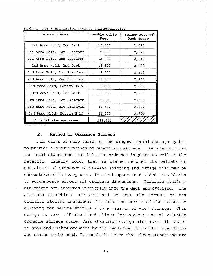
Table 1 AOE 6 Ammunition Storage Characteristics
Storage Area Usable Cubic Feet
Square Feet of Deck Space
1st Ammo Hold, 2nd Deck 12,300 2,070
1st Ammo Hold, 1st Platform 12,300 2,070
1st Ammo Hold, 2nd Platform 12,200 2, 010
2nd Ammo Hold, 2nd Deck 13,600 2,240
2nd Ammo Hold, 1st Platform 13,600 2,240
2nd Ammo Hold, 2nd Platform 11,900 2,240
2nd Ammo Hold, Bottom Hold 11,800 2,200
3rd Ammo Hold, 2nd Deck 12,550 2,220
3rd Ammo Hold, 1st Platform 13,600 2,240
3rd Ammo Hold, 2nd Platform 11,600 2,240
3rd Ammo Hold, Bottom Hold 11,500 2,200
11 total storage areas 136,950 V///////////S.
2. Method of Ordnance Storage
This class of ship relies on the diagonal metal dunnage system
to provide a secure method of ammunition storage. Dunnage includes
the metal stanchions that hold the ordnance in place as well as the
material, usually wood, that is placed between the pallets or
containers of ordnance to prevent shifting and damage that may be
encountered with heavy seas. The deck space is divided into blocks
to accommodate almost all ordnance dimensions. Portable aluminum
stanchions are inserted vertically into the deck and overhead. The
aluminum stanchions are designed so that the corners of the
ordnance storage containers fit into the corner of the stanchion
allowing for secure storage with a minimum of wood dunnage. This
design is very efficient and allows for maximum use of valuable
ordnance storage space. This stanchion design also makes it faster
to stow and unstow ordnance by not requiring horizontal stanchions
and chains to be used. It should be noted that these stanchions are
new and have not yet been tested in the fleet [Ref. 14: pp. 42-44
and Ref. 15].
D. STORES AND PROVISIONS
The fourth hold, the one farthest aft, is for the storage of
dry, refrigerated and frozen goods. This hold has four levels with
the top level, the second deck, being used for dry stores. The
lower three levels are for chilled and frozen goods. The fourth
hold is serviced by one 12,000 pound elevator and a pallet
conveyor, both centerlined to maximize utilization. The pallet
conveyor is rated to carry 3,000 pound, palletized loads [Ref. 14:
p. 49]. The total storage area is 90,400 cubic feet, of which
54,000 is refrigerated [Ref. 5: p. B-l], with an expected stow
factor of .8. This compares to the AOE-1 class which has 105,000
cubic feet of stores with 60,000 being refrigerated [Ref. 5: p. B-
2] .
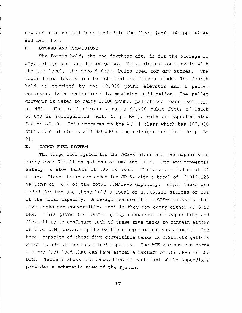
E. CARGO FUEL SYSTEM
The cargo fuel system for the AOE-6 class has the capacity to
carry over 7 million gallons of DFM and JP-5. For environmental
safety, a stow factor of .95 is used. There are a total of 24
tanks. Eleven tanks are coded for JP-5, with a total of 2,812,225
gallons or 40% of the total DFM/JP-5 capacity. Eight tanks are
coded for DFM and these hold a total of 1,963,213 gallons or 30%
of the total capacity. A design feature of the AOE-6 class is that
five tanks are convertible, that is they can carry either JP-5 or
DFM. This gives the battle group commander the capability and
flexibility to configure each of these five tanks to contain either
JP-5 or DFM, providing the battle group maximum sustainment. The
total capacity of these five convertible tanks is 2,281,462 gallons
which is 30% of the total fuel capacity. The AOE-6 class can carry
a cargo fuel load that can have either a maximum of 70% JP-5 or 60%
DFM. Table 2 shows the capacities of each tank while Appendix D
provides a schematic view of the system.
17
Table 2 Cargo Fuel Tank Capacities
Compartment Number 100% Capacity In Gallons 100 % Capacity in Barrels
7-44-0-JJ 108,365 2,408
7-105-0-JJ 386,333 8,585
7-205-0-JJ 18,533 412
7-205-1-JJ 305,753 6,795
7-205-2-JJ 340,764 7,513
7-297-2-JJ 283,340 6,296
7-297-1-JJ 283,335 6,296
7-265-2-JJ 228,921 5,087
7-265-1-JJ 228,917 5,087
7-362-1-JJ 313,981 6,977
7-362-2-JJ 313,983 6,977
7-65-0-FF 336,200 7,471
7-245-0-FF 213,334 4,740
7-395-2-FF 282043 6,268
7-395-1-FF 282,040 6,268
7-425-2-FF 226,404 5,031
7-425-1-FF 226,400 5,031
7-430-0-FF 24,758 550
7-565-0-FF 372,034 8,267
7-150-0-FF/JJ 791,754 17,595
7-265-0-FF/JJ 445,200 9,893
7-330-0-FF/JJ 445,195 9,893
7-330-2-FF/JJ 299,658 6,659
7-330-1-FF/JJ 299,655 6,659
Total of 24 Tanks 7,056,900 ^^^^
Note: JJ are coded to convertible.
carry JP-5, FF carry only DFM and JJ/FF are
For these convertible tanks to be a useful asset, commanders
must understand the process to convert a tank from one fuel system
to the other. Each of the convertible tanks has the necessary 10
18
to 12 feet of piping to connect it with either the DEM or JP-5 fuel
pumping system. This piping is copper-nickel for the DFM system
and steel for the JP-5 system. If the tank is designated to carry
JP-5, the tank must be opened, gas freed and ship's force personnel
must enter the tank. A blank flange is placed on the DFM suction
piping and the blank flange from the JP-5 suction piping is
removed. The most time consuming portion of this process if the
tank is empty is to certify the tank to be gas freed [Ref. 18].
After the piping has been properly aligned, the cargo fuel control
console will be updated to show that this tank is now a JP-5 tank.
If the tank is being converted from DFM to JP-5, additional time
will be spent flushing and "mucking" out the tank prior to
introducing JP-5. This step is necessary to maintain the quality
standard of the JP-5. This step is not necessary when converting
from JP-5 to DFM [Ref. 18].
The decision of which fuel to place in each tank is based on
the propulsion of the aircraft carrier and number of escorts
assigned. If the carrier is nuclear powered, more JP-5 can be
carried vice DFM. The actual decision is made by the immediate
superior type commander, usually the Logistics Group (LOGGRU ONE on
the west coast, LOGGRU TWO on the east coast) for that operating
area. This decision will be made after consulting with the Battle
Group commander and the Surface Type Commander (SURFPAC or
SURFLANT).
The AOE-6 class has a total of nine cargo fuel oil pumps, five
for DFM and four for JP-5. Each pump has a 3,000 gallons per
minute capacity. While the AOE-6 can fuel other ships from both
sides, they can only receive CONSOL cargo fuel from three double
hose receiving stations on the starboard side of the ship [Ref. 5:
p. B-l] .
While the AOE-6 class is designed to carry 21,000 barrels of
fuel less then the AOE-1 class, a very important design feature was
incorporated into the AOE-6. The AOE-1 is designed so that the
19
cargo JP-5 is stored in the forward part of the ship. The cargo
DFM is stored in the midships area. A constraint is placed on how
large a difference can exist between the quantities of JP-5 to DFM
because of stress to the hull caused by hogging and sagging. In an
operational setting, sea water ballast can be used to fill this
constraint. The AOE-6 does not have this constraint because the
JP-5 tanks and DFM tanks are interspersed throughout the ship to
prevent this problem as clearly shown in Appendix D. The
constraint placed upon the AOE-6 is that the ship begins to lose
stability as it approaches 30% of its liquid load. Again, sea
water ballast can be used to compensate for this constraint. Both
the AOE-1 and the AOE-6 classes have the ability to co-mingle
bunker and cargo fuels.
20
III. SCENARIO DEVELOPMENT
The scenario developed for this thesis is designed to test the
capabilities of the AOE-6 class station ship. This model was not
developed to test a specific real-world threat, but is intended to
demonstrate commodity usage for a CVBG during various phases of a
possible future operation. The specific ship combinations are
intended to reflect what would be considered a typical CVBG and ARG
and provide useful information concerning commodity usage rates and
resupply of forces afloat.
A. GENERAL CONCEPT
This scenario is based on historic use of the aircraft carrier
and escorts in the roles of sea control, power projection ashore
and demonstrating national interest by "showing the flag" abroad.
The starting point for this scenario is a forward deployed nuclear
powered aircraft carrier and six gas turbine powered escorts. The
escorts include two Ticonderoga class cruisers, two Burke class
destroyers, one Spruance class destroyer and one Kidd class guided
missile destroyer. The CVBG is inport at an overseas United States
Naval Facility that is co-located with a weapons station. One
AOE-6 class fast combat stores ship is assigned to the battle group
to serve as the station ship. A situation has developed in a
region of the world that requires the carrier battle group to sail
immediately to that area to show an American presence and await
follow on tasking.
1. Description of Scenario
The United States is about to become involved in a possible
regional conflict. The carrier battle group is currently inport
but has been ordered to sortie and proceed to the region. It will
take 10 days for the battle group to arrive. The ALSS has been
reactivated and supplies are already being pushed into the theater.
In an effort to influence events without hostilities and to
show United States resolve, the carrier battle group will proceed
to a station 100 miles off the coast of the troublesome region and
conduct a presence mission while at the same time gearing up for
possible combat operations. This presence mission will last for 30
21
days.
When diplomacy fails the carrier battle group will be ordered
to conduct combat operations. The mission of the CVBG will be to
conduct strike operations (including naval gunfire support) against
enemy bases preceding an amphibious invasion, with a secondary
missions of neutralizing enemy submarines, establishing air and sea
superiority and attacking possible enemy resupply routes.
Current intelligence indicates a medium ASW threat due to the
recent delivery of several diesel submarines, a high ASUW threat
comprised mainly of aggressive patrol craft and land based cruise
missiles. A high AAW threat is largely due to the recent purchase
and delivery of an undetermined number of fourth generation Ex-
Soviet Union fighter and attack aircraft. The enemy has good air
search radar and an adequate air defense missile system.
This scenario (Scenario 1) is intended to demonstrate how an
AOE-6 with a nominal weapons loadout can proceed to a weapons
facility and complete an onload of weapons determined to give
maximum benefit to the battle group. This benefit is based upon a
method of prioritization of each ordnance type that will be
discussed in Chapter IV. This problem is realistic in the sense
that AOEs currently deploy loaded at 80% usable capacity [Ref. 15].
The battle group will then proceed on an extended operation. The
8 0 day operation will be divided into three phases: transit,
presence and combat. Each of the first phase, transit, will last
10 days, while the presence phase will last 3 0 days. The final
phase, combat, will last 40 days. One of the purposes of modeling
the CVBG during an extended operation is to find the optimal mix
of JP-5 and DFM that will allow the battle group to proceed through
the 80 day operation with a minimum number of CONSOLS between the
station ship and shuttle ships.
The first modification to this scenario (Scenario 1A) will be
to replace the nuclear powered aircraft carrier with a fossil fuel
powered aircraft carrier. The second modification will be to have
a three ship ARG join the CVBG in the operation. Scenario IB will
have a nuclear powered carrier while scenario 1C will have a fossil
22
fuel powered carrier. The purpose of these modifications is to
determine the impact on the number and frequency of CONSOL
replenishments that will be required during the operation and
determine if there is a change in the recommended mix of DFM and
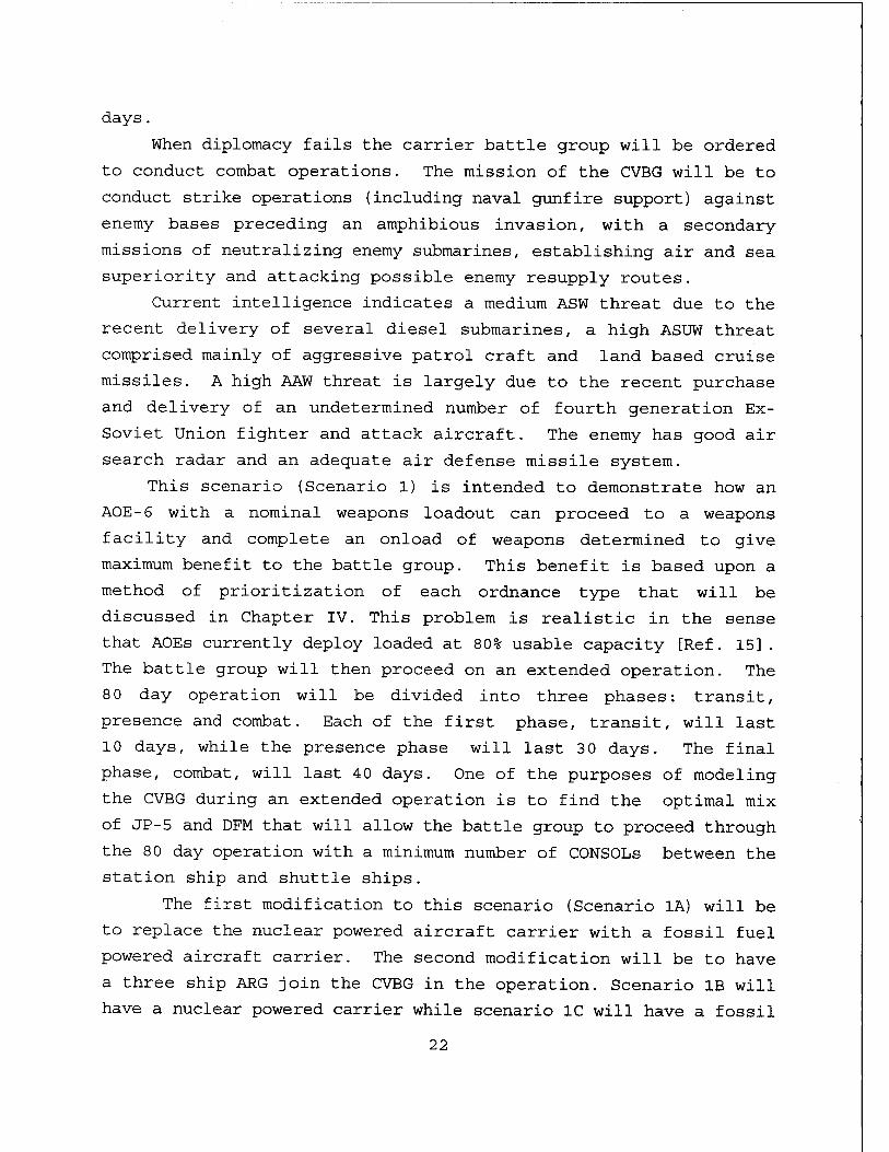
JP-5 to carry. Table 3 shows the ship combinations in each
scenario modification:
Table 3 Battle Group Composition
Forces Scenario 1 Scenario 1A Scenario IB Scenario 1C
Involved
CV Type CVN-68 class CV - 63 class CVN-68 class CV - 63 class
Escorts 2 CG-47 class 2 CG-47 class 2 CG-47 class 2 CG-47 class
2 DDG-51 class 2 DDG-51 class 2 DDG-51 class 2 DDG-51 class
1 DD-963 class 1 DD-963 class 1 DD-963 class 1 DD-963 class
1 DDG-993 class 1 DDG-993 class 1 DDG-993 class 1 DDG-993 class
Station 1 AOE-6 class 1 AOE-6 class 1 AOE-6 class 1 AOE-6 class
Ship
Amphibious NONE NONE 1 LHA 1 LHA
Forces l LPD-4 class
1 LSD-41 class
Embarked MEU
1 LPD-4 class
1 LSD-41 class
Embarked MEU
B. DATA BASE SPECIFICS
The purpose of this section is to clearly lay out for the
reader the data that will later be used in the model formulation.
This data will provide insight into the process that a logistics
planner uses in determining the resupply requirements of a battle
group. Based on this operational scenario and the data shown in
this section, a model will be formulated to track and resupply
four major commodities: DFM, JP-5, ordnance and stores. All of
these commodities will be tracked as a whole in the battle group.
Specifically in this section, the maximum quantity of each
commodity possible at any time in the battle group as well as the
battle group's daily commodity usage rate in each phase of the
operation will be highlighted.
23
1. DFM
The maximum DFM available to the battle group involved in each
scenario is found by summing the maximum fuel capacity for each
ship in the scenario and adding the cargo fuel from the station
ship and multiplying by the stow factor for fuel, .95. The stow
factor for fuel is a safety factor for the environment to prevent
fuel from being discharged into the ocean. In order to keep this
document from being classified, the ship class fuel capacities used
in this model are taken from the Unclassified TACLOGS Database
[Ref. 27].
The battle group DFM daily usage rates are derived by sumv -.g
the fuel consumed by the entire battle group for an average sj d
per day. During the scenario the following speeds will be used. e
average transit speed will be 20 knots, 16 knots when operat.. j
with the ARG. The average presence, or patrolling, speed will ■; 12 knots and the average combat speed will be 16 knots for t,ie
carrier battle group and remain 12 knots for the ARG [Ref. 8: p.
22] . Daily ship fuel usage figures are derived from Naval
Postgraduate Technical Report, Predicting Ship Fuel Consumption
[Ref. 6]. Table 4 shows the daily fuel consumption for individual
ship classes during the three phases of the operation as well as
the maximum individual ship class fuel capacities. Table 5 shows
the maximum DFM available to the battle group in each scenario as
well as the battle group's daily usage rate for each phase of the
scenario.
24
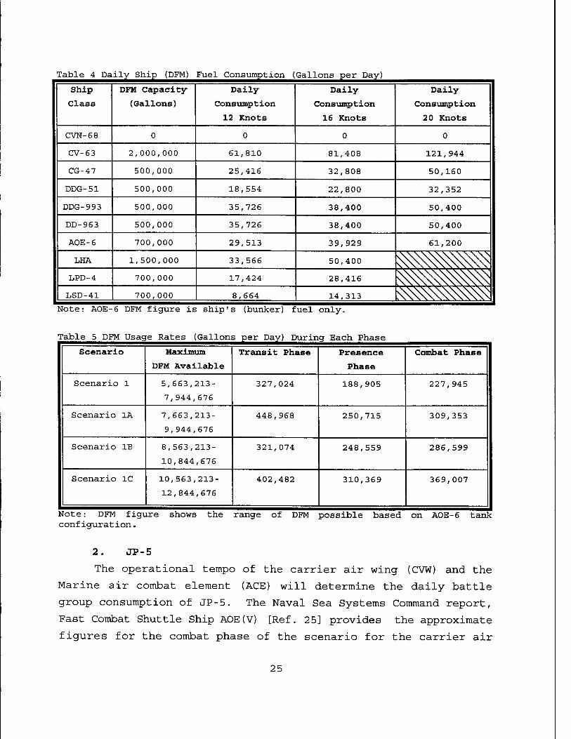
Table 4 Da ily Ship (DFM) Fuel Consumption (Gallons per Day)
Ship
Class
DFM Capacity
(Gallons)
Daily
Consumption
12 Knots
Daily
Consumption
16 Knots
Daily
Consumption
20 Knots
CVN-68 0 0 0 0
CV-63 2,000,000 61,810 81,408 121,944
CG-47 500,000 25,416 32,808 50,160
DDG-51 500,000 18,554 22,800 32,352
DDG-993 500,000 35,726 38,400 50,400
DD-963 500,000 35,726 38,400 50,400
AOE-6 700,000 29,513 39,929 61,200
LHA 1,500,000 33,566 50,400 <^^^ LPD-4 700,000 17,424 28,416 ^^^ LSD-41 700,000 8,664 14,313 ^^^^
Note: AOE-6 DFM figure is ship's (bunker) fuel only.
Table 5 DFM Usag re Rates (Gallons per Day) During Each Phase
Scenario Maximum
DFM Available
Transit Phase Presence
Phase
Combat Phase
Scenario 1 5,663,213-
7,944,676
327,024 188,905 227,945
Scenario 1A 7,663,213-
9,944,676
448,968 250,715 309,353
Scenario IB 8,563,213-
10,844,676
321,074 248,559 286,599
Scenario 1C 10,563,213-
12,844,676
402,482 310,369 369,007
Note: DFM figure shows the range of DFM possible based configuration.
on AOE-6 tank
2. JP-5
The operational tempo of the carrier air wing (CVW) and the
Marine air combat element (ACE) will determine the daily battle
group consumption of JP-5. The Naval Sea Systems Command report,
Fast Combat Shuttle Ship AOE(V) [Ref. 25] provides the approximate
figures for the combat phase of the scenario for the carrier air
25
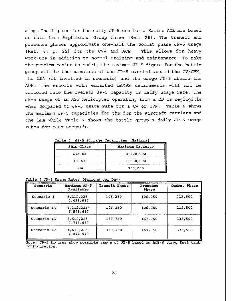
wing. The figures for the daily JP-5 use for a Marine ACE are based
on data from Amphibious Group Three [Ref. 28] . The transit and
presence phases approximate one-half the combat phase JP-5 usage
[Ref. 8: p. 22] for the CVW and ACE. This allows for heavy
work-ups in addition to normal training and maintenance. To make
the problem easier to model, the maximum JP-5 figure for the battle
group will be the summation of the JP-5 carried aboard the CV/CVN,
the LHA (if involved in scenario) and the cargo JP-5 aboard the
AOE. The escorts with embarked LAMPS detachments will not be
factored into the overall JP-5 capacity or daily usage rate. The
JP-5 usage of an ASW helicopter operating from a DD is negligible
when compared to JP-5 usage rate for a CV or CVN. Table 6 shows
the maximum JP-5 capacities for the for the aircraft carriers and
the LHA while Table 7 shows the battle group's daily JP-5 usage
rates for each scenario.
Table 6 JP-5 Storage Capacities (Gallons)
Ship Class Maximum Capacity
CVN-68 2,400,000
CV-63 1,500,000
LHA 300,000
Table 7 JP-5 Usage Rates (Gallons per Day)
Scenario Maximum JP-5 Available
Transit Phase Presence Phase
Combat Phase
Scenario 1 5,212,225- 7,493,687
106,250 106,250 212,500
Scenario 1A 4,312,225- 6,593,687
106,250 106,250 212,500
Scenario IB 5,512,225- 7,793,687
167,750 167,750 335,500
Scenario 1C 4,612,225- 6,893,687
167,750 167,750 335,500
Note: JP-5 figures show possible range of JP-5 based on AOE-6 cargo fuel tank configuration.
26
3. Ordnance
At the beginning of the scenario, the AOE will moving to a
Naval Magazine to conduct a weapons onload. One important aspect
of loading ordnance on a CLF ship is that the main constraints to
loading are volume, measured in cubic feet, and compatibility.
However, expenditure rates are usually measured by weight (tons) of
the ordnance spent. The model to load weapons will look at all
constraints, including weight and volume, while the second model
that tracks commodities available to the battle group on a daily
basis, will track ordnance in tons. For the AOE-6 class, the
designed maximum ordnance capacity is 1,800 tons [Ref. 5: p. B-l].
This design capacity does not include a stow factor.
While the AOE represents a portion of the ordnance carried in
the battle group, aircraft carriers carry even larger quantities of
ordnance. Each ship in the battle group will also be fully loaded
prior to sailing. The maximum ordnance available for any scenario
will be the summation of all the individual ship weapons capacities
as well as the cargo ordnance available from the AOE. Once the
AOE-6 onload is complete and the battle group has left port,
ordnance will be expended as a single commodity measured in tons.
Table 8 provides a look at the ordnance tonnage available for each
ship class in the battle group. Table 9 provides a look at the
total ordnance tonnage when the battle group is fully armed for
each scenario as well as the planned expenditure rates for each
phase of the operation. The ordnance figures for the ship classes
are taken from the Unclassified TACLOGS Database [Ref. 27] and are
estimates based upon the weapon weights of a notional loadout.
The AOE(V) study [Ref. 25] and the 1993 thesis by LT. Reeger
[Ref. 8] also provide guidance for the daily rate of ordnance
expenditures. The usage rate for this model will be 10 tons per day
during the presence phase and 100 tons of ordnance per day during
the combat phase [Ref. 8: p 23, Ref. 25: p. 22]. For the combat
phase, this is half the strike ordnance used per carrier per day
during the Vietnam War and reflects the preponderance of "smart"
weapons in the current ordnance inventory [Ref. 8: p.23]. This
27
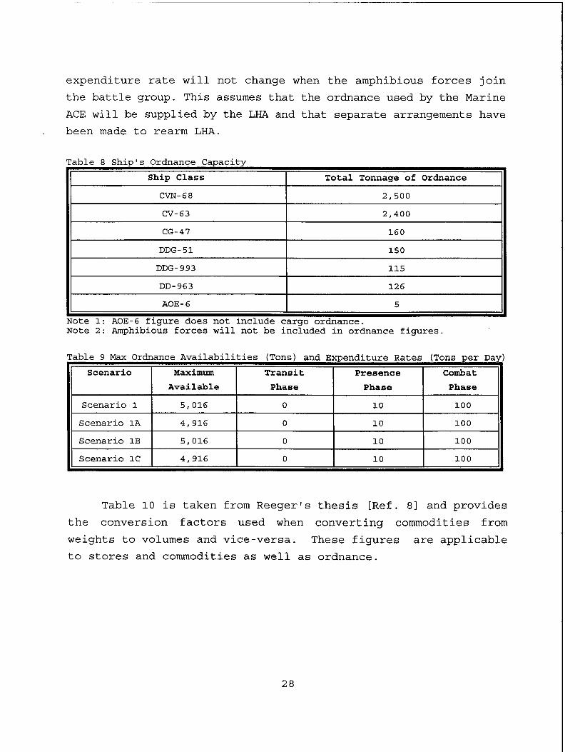
expenditure rate will not change when the amphibious forces join the battle group. This assumes that the ordnance used by the Marine ACE will be supplied by the LHA and that separate arrangements have been made to rearm LHA.
Table 8 Ship's Ordnance Capacity
Ship Class Total Tonnage of Ordnance
CVN-68 2,500
CV-63 2,400
CG-47 160
DDG-51 150
DDG-993 115
DD-963 126
AOE-6 5
Note 1: AOE-6 figure does not include cargo ordnance. Note 2: Amphibious forces will not be included in ordnance figures.
Table 9 Max Ordnance Availabili ties (Tons) and Expenditure Rates (Tons per Day]
Scenario Maximum
Available
Transit
Phase
Presence
Phase
Combat
Phase
Scenario 1 5,016 0 10 100
Scenario 1A 4,916 0 10 100
Scenario IB 5,016 0 10 100
Scenario 1C 4,916 0 10 100
Table 10 is taken from Reeger's thesis [Ref. 8] and provides the conversion factors used when converting commodities from weights to volumes and vice-versa. These figures are applicable to stores and commodities as well as ordnance.
28
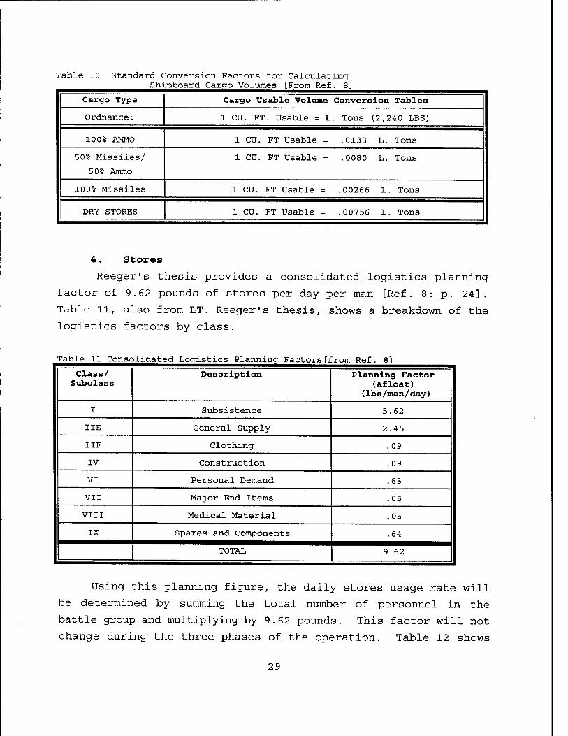
Table 10 Standard Conversion Factors for Calculating Shipboard Cargo Volumes [From Ref. 8]
Cargo Type Cargo Usable Volume Conversion Tables
Ordnance: 1 CU. FT. Usable = L. Tons (2,240 LBS)
100% AMMO 1 CU. FT Usable = .0133 L. Tons
50% Missiles/
50% Ammo
1 CU. FT Usable = .0080 L. Tons
100% Missiles 1 CU. FT Usable = .00266 L. Tons
DRY STORES 1 CU. FT Usable = .00756 L. Tons
4. Stores
Reeger's thesis provides a consolidated logistics planning
factor of 9.62 pounds of stores per day per man [Ref. 8: p. 24].
Table 11, also from LT. Reeger's thesis, shows a breakdown of the
logistics factors by class.
Table 11 Consolidated Logistics Planning Factors[from Ref. 8]
Class/ Subclass
Description Planning Factor (Afloat)
(lbs/man/day)
I Subsistence 5.62
HE General Supply- 2.45
IIF Clothing .09
IV Construction .09
VI Personal Demand .63
VII Major End Items .05
VIII Medical Material .05
IX Spares and Components .64
TOTAL 9.62
Using this planning figure, the daily stores usage rate will
be determined by summing the total number of personnel in the
battle group and multiplying by 9.62 pounds. This factor will not
change during the three phases of the operation. Table 12 shows
29
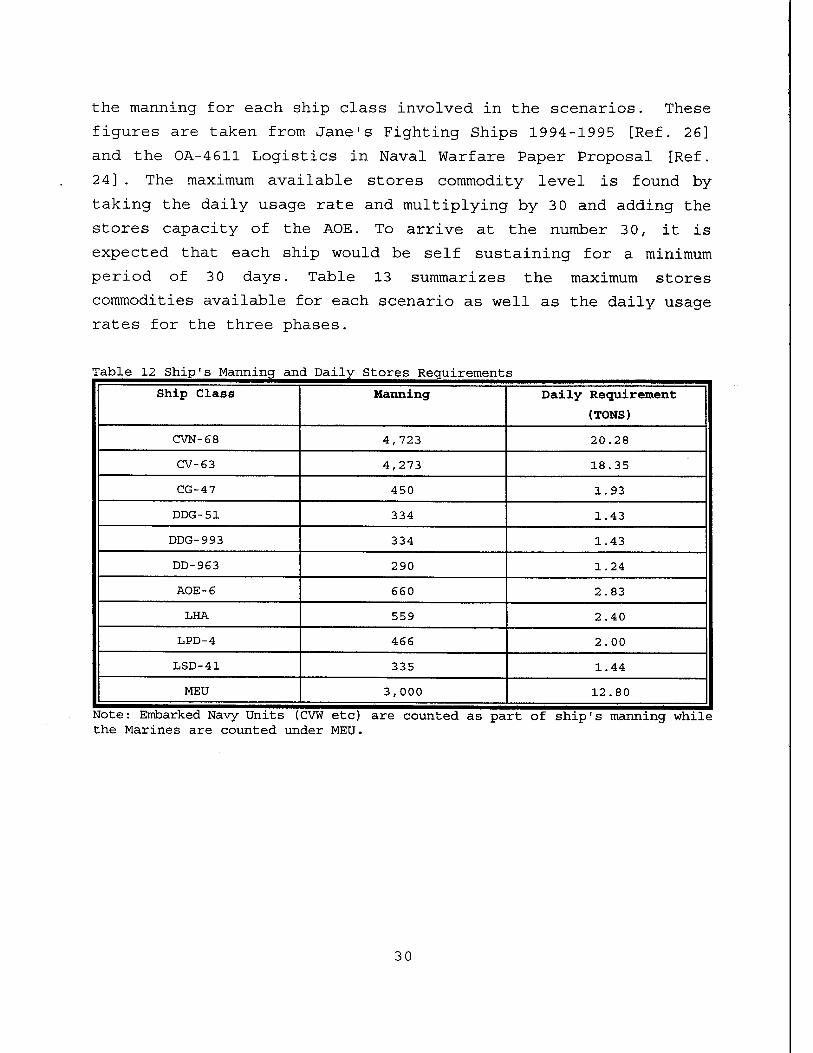
the manning for each ship class involved in the scenarios. These
figures are taken from Jane's Fighting Ships 1994-1995 [Ref. 26]
and the OA-4611 Logistics in Naval Warfare Paper Proposal [Ref.
24] . The maximum available stores commodity level is found by-
taking the daily usage rate and multiplying by 3 0 and adding the
stores capacity of the AOE. To arrive at the number 30, it is
expected that each ship would be self sustaining for a minimum
period of 30 days. Table 13 summarizes the maximum stores
commodities available for each scenario as well as the daily usage
rates for the three phases.
Table 12 Ship's Manning and Daily Stores Requirements
Ship Class Manning Daily Requirement
(TONS)
CVN-68 4,723 20.28
CV-63 4,273 18.35
CG-4 7 450 1.93
DDG-51 334 1.43
DDG-993 334 1.43
DD-963 290 1.24
AOE-6 660 2.83
LHA 559 2.40
LPD-4 466 2.00
LSD-41 335 1.44
MEU 3,000 12.80
Note: Embarked Navy Units (CVW etc) are counted as part of ship's manning while the Marines are counted under MEU.
30
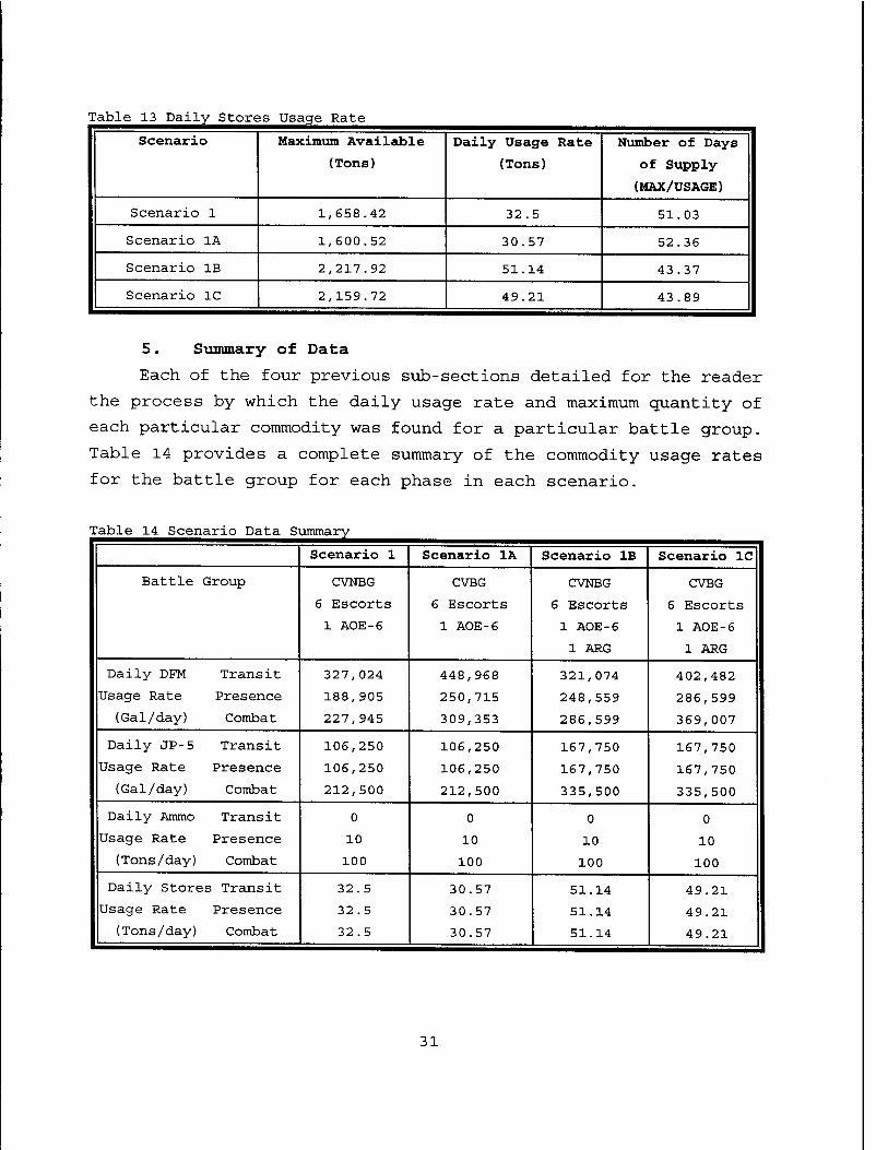
Table 13 Daily Stores Usage Rate
Scenario Maximum Available
(Tons)
Daily Usage Rate
(Tons)
Number of Days
of Supply
(MAX/USAGE)
Scenario 1 1,658.42 32.5 51.03
Scenario 1A 1,600.52 30.57 52.36
Scenario IB 2,217.92 51.14 43.37
Scenario 1C 2,159.72 49.21 43.89
5 . Summary of Data
Each of the four previous sub-sections detailed for the reader
the process by which the daily usage rate and maximum quantity of
each particular commodity was found for a particular battle group.
Table 14 provides a complete summary of the commodity usage rates
for the battle group for each phase in each scenario.
Table 14 Scenario Data Summary
Scenario 1 Scenario 1A Scenario IB Scenario 1C
Battle Group CVNBG CVBG CVNBG CVBG
6 Escorts 6 Escorts 6 Escorts 6 Escorts
1 AOE-6 1 AOE-6 1 AOE-6
1 ARG
1 AOE-6
1 ARG
Daily DFM Transit 327,024 448,968 321,074 402,482
Usage Rate Presence 188,905 250,715 248,559 286,599
(Gal/day) Combat 227,945 309,353 286,599 369,007
Daily JP-5 Transit 106,250 106,250 167,750 167,750
Usage Rate Presence 106,250 106,250 167,750 167,750
(Gal/day) Combat 212,500 212,500 335,500 335,500
Daily Ammo Transit 0 0 0 0
Usage Rate Presence 10 10 10 10
(Tons/day) Combat 100 100 100 100
Daily Store s Transit 32.5 30.57 51.14 49.21
Usage Rate Presence 32.5 30.57 51.14 49.21
(Tons/day) Combat 32.5 30.57 51.14 49.21
31
C. SCENARIO ASSUMPTIONS
Several assumptions are made about the scenario in order to
isolate the AOE. The goal here is to assure that all logistics
support for the battle group flows through the AOE.
* Forward support basing (ALSS) is fully operational.
* Sea and airlift is available to fully supply the ALSS from
the United States .
* Enough single product shuttle ships are available to move
commodities from the ALSS to the battle group station ship.
* CONSOL operations will occur when any single commodity
reaches the minimum level for the battle group. All
commodities will then be replenished to the maximum capacity
for the battle group. The single commodity shuttle ships
will all load, transit, UNREP and return to port
simultaneously.
* Every ship will start the scenario fully fueled, armed and
resupplied, including the AOE.
* The ARG will consist of one LHA, one LPD and one LSD with an
embarked Marine Expeditionary Unit (MEU) of 3,000 Marines,
six Harriers, and 26 Marine helicopters embarked.
* The AOE will supply the ARG with fuel and provisions only.
32
IV. SURVEY
The purpose of this survey is to demonstrate a method of
prioritizing the relative value for each type of ordnance utilized
in the survey. Only by assigning a certain benefit, or "utility",
to each weapon, can an "optimal" load list, or solution be
generated by a linear program. A primary focus of this thesis is
the development of a model that will load ordnance aboard a ship,
based on the physical characteristics of the ship and the ordnance.
This thesis is not however, focused on the optimal method of
finding the relative benefit for each ordnance type. As such,
decreasing marginal returns are not utilized in this model. This
fact is partially compensated for by assigning a minimium and
maximum number of each weapon that can be loaded.
The loadout for any ammunition carrying ship is shown on a
document called a tailored load list. This document lists the
variety and quantity of the various products carried by the ship
[Ref. 23] . The tailored load list used as a planning aid in this
thesis is the USS Seattle's tailored load list for her 1995
deployment [Ref. 23]. Remembering that the main function of the AOE
is to support the CVBG, including the embarked air wing, a load
planning conference is held to determine which weapons and in what
quantity, are to be carried by the AOE. The main participants in
the conference are the aircraft carrier's ordnance officers, the
deploying battle group commander's and air wing's strike
operations people and the surface type commander [Refs. 15 and 22].
Their job is to develop a clear concise list of weapons they desire
the AOE to carry in order to resupply the CVBG. The surface type
commander is involved to ensure that adequate resupply is available
for the escorts traveling with the carrier.
Thanks in large part to the Persian Gulf War, models based on
recent experience exist to accurately predict ordnance expenditures
during combat operations. However, in today's fast changing world,
a deploying battle group has no way of knowing what type of
33
operation they will become involved in. This means the CVBG must
carry a variety, over 300 line items, of ordnance and accompanying
accessories. For the purpose of this survey, 21 weapons were
selected from a current AOE tailored load list [Ref. 23] for use in
the given scenario. One consideration given to what ordnance will
be included on the survey list is that weapons that could not be
loaded, reloaded, fired or transferred at sea would not be
included. Such important weapons as Tomahawk cruise missiles, ship
launched (canister) Harpoon anti-ship missiles and vertically
launched SM-2 missiles fall into this category. The second,
subjective, consideration is that the weapon must have well known
employment features to a "majority" of aviation and surface warfare
qualified naval officers polled in the survey.
As stated previously, the goal of this survey is to develop a
method of prioritization. This is done by establishing a minimal
ordnance loadout, that is a minimum number of each of the 21 weapon
types chosen for the survey, aboard the AOE-6 to respond to the
most likely contingencies a deploying CVBG would encounter. This
minimal loadout is in effect the minimum number of each weapon that
will be carried aboard the AOE and is transparent to the survey
respondent. This minimal ordnance level is determined randomly by
the modeler, in this case the author, to force the AOE to carry a
minimum of each of the 21 weapon types. It does not, nor is it
intended, to reflect a given percentage of the AOE loadout. To
attempt to try to pre-load the AOE with a given percentage, based
solely on the limited number of weapon types would be unrealistic.
A warfare qualified naval officer is then provided a combat
scenario in which that officer will determine which weapons that
individual feels would be most useful given the particular
scenario. A maximum level for each weapon is set to prevent the
model from filling the AOE with a large number of high priority
weapons. Should the mission tasking change to an open ocean ASW
threat, the minimum (and maximum) levels for weapons such as MK-46
and Sonobouys would rise, while the minimum (and maximum) level for
34
Hellfire missiles may drop. The process is modeled after the load
conference, with one person, the author, playing the role of the
conference participants. This method of setting minimums and
maximums also replicates the power that Fleet and CVBG commanders
have to modify load lists.
The naval officer's survey responses are used to assign
weights or values to the different types of ordnance. The ordnance
loading model will then provide an optimum load list, based on the
ordnance values, detailing the number of each weapon type to load
and the storage area to place the weapon in, staying within the
volume, weight and compatibility constraints of the AOE-6. Naval
Weapons Station, Earle, NJ still uses the pencil and paper method
of determining where on the ammunition ship to place ordnance to
meet all the constraints involved in ordnance storage [Ref. 15].
The loading of ordnance on the ship accomplished by the first
computer model will look at five factors. Four of the factors,
weight, volume, compatibility and required accessories are already
determined. The fifth factor is benefit. This survey will scale
each ordnance type of the 21 in the survey and give a scaled
benefit for that ordnance type. These scaled benefit values will
then be transformed to an ordinal scale, from 1 to 100 to be used
in the objective function of the model. The objective function for
this model will be to maximize the benefit to the battle group of
the entire CLF ship weapon loadout. This survey will afford the
individual officers the opportunity to use their experience and
judgment in deciding which ordnance types are most favorable to
have for immediate resupply of the battle group.
A. SURVEY METHODOLOGY
The survey instructions, Appendix E, and the survey, Appendix
F, were designed to provide a method to determine a prioritization
of ordnance to be loaded in the ammunition holds of the AOE-6 class
ship. The survey format is based one developed by Guadalupe [Ref.
12] , and used by Rowland [Ref. 9] . The forms were distributed
evenly between officers at NPS and officers in current fleet
35
operational billets. The goal was to survey officers with
backgrounds in carrier battle group operations. Individuals such
as carrier air wing pilots and naval flight officers as well as
surface warfare officers were sought. Fleet surveys were sent to
aircraft carriers, carrier air wings, commanding officers of
cruisers and destroyers and various aircraft squadron commanding
officers.
A categorical method ( developed by Lindsay [Ref. 11] and used
by Rowland [Ref. 9]) was employed to elicit preferences between the
different ordnance types. The categorical method also makes it
easy for both the person doing the survey and grading the survey to
use. The categories used to prioritize the ordnance were
1. very low,
2. low,
3. medium,
4. high, and
5. great contribution to the CVBG mission accomplishment.
1. Ordnance
The survey form listed 21 types of ordnance for evaluation.
The person responding to the survey placed a mark in the
appropriate category. While a tailored load list may have over 300
line items, the list was pared down by choosing ordnance that could
be used and loaded while remaining at sea and choosing mostly
threat ordnance for evaluation.
B. SURVEY QUESTIONNAIRE STATISTICS
A total of 100 survey forms were sent out, of which 77 were
completed and returned. The Survey Information Questionnaire,
Appendix G, provided information about the officer completing the
survey as well as comments about the survey:
The 77 returned surveys included inputs from 53 lieutenants,
15 lieutenant commanders, eight commanders and one captain. By
designator, the breakdown included 3 8 surface warfare officers, 19
pilots and 20 naval flight officers. The average number of years
spent on active duty in the survey was 10.6 years, with an average
of less than one year of staff duty.
36
The comments concerning the survey indicate that the basic
scenario was understandable. The majority of specific comments
came from fleet aviators and naval flight officers. The main focus
of these comments centered on the desire for more detailed enemy
orders of battle and information on specific targets. The most
common comment was for more information on the ratio of "hard"
targets to "soft" targets. In reality, more detailed information
will be available on specific targets so this comment is a fair
one. One other respondent desired more information about the air
wing composition.
Of the 21 weapons rated in the survey, ASROC, MK 4 6 torpedoes
and MK 60 Captor mines were the weapons that survey takers wanted
to drop from the weapons load list. One specific comment was to
allow land based P-3 and B-52 aircraft conduct offensive mining if
necessary. Most officers felt that the use of rail launched ASROC
is now limited to only one class of ship (DDG-993) so this weapon
could be dropped.
The most common weapon that survey takers wanted added to the
survey weapons list was the Advanced Medium Range Air to Air
Missiles (AMRAAM). This weapon is actually an Air Force design
that is currently being added to the Navy arsenal. While not part
of the USS Seattle tailored load list, it is anticipated that it
will soon become part of the load list for future deploying battle
groups. Other weapons mentioned to add included laser guided
bombs, which actually are not weapons, but a fin set and guidance
package for the MK 80 series bombs, MK 50 torpedoes (to replace MK
4 6 torpedoes), Gator mines, SLAM missiles and 25 MM Chain Gun
ammunition.
The majority of comments made were very constructive. As
expected, the most detailed comments came from officers with a
strike warfare background. These officers were very informative on
the detailed process a strike operations planner goes through prior
37
to launching aircraft. They were very concerned with the level of
detail of the survey and felt they had to make too many assumptions
with their answers. Again, it must be remembered that the focus of
this project is to develop a model to load ordnance, not develop
the best method of determining weapon utility. In an actual
scenario, the strike mission planners will have adequate time to
develop a more detailed prioritization method to work with.
C. RAW FREQUENCY DATA
Table 15 shows the results for survey responses, with the
weapon type being listed down the left column and the contribution
categories listed across the top:
38
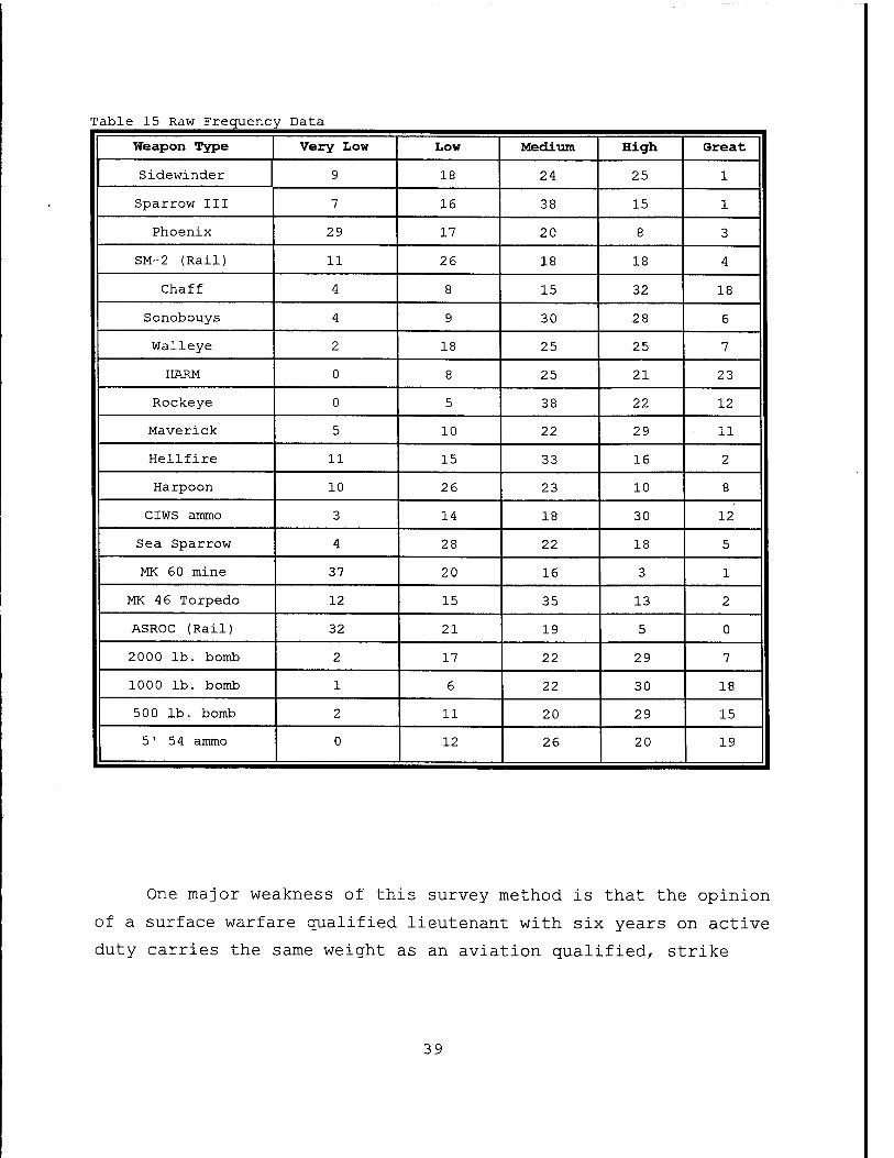
Table 15 Raw Frequency Data
Weapon Type Very Low Low Medium High Great
Sidewinder 9 18 24 25 1
Sparrow III 7 16 38 15 1
Phoenix 29 17 20 8 3
SM-2 (Rail) 11 26 18 18 4
Chaff 4 8 15 32 18
Sonobouys 4 9 30 28 6
Walleye 2 18 25 25 7
HARM 0 8 25 21 23
Rockeye 0 5 38 22 12
Maverick 5 10 22 29 11
Hellfire 11 15 33 16 2
Harpoon 10 26 23 10 8
CIWS ammo 3 14 18 30 12
Sea Sparrow 4 28 22 18 5
MK 60 mine 37 20 16 3 1
MK 46 Torpedo 12 15 35 13 2
ASROC (Rail) 32 21 19 5 0
2000 lb. bomb 2 17 22 29 7
1000 lb. bomb 1 6 22 30 18
500 lb. bomb 2 11 20 29 15
5' 54 ammo 0 12 26 20 19
One major weakness of this survey method is that the opinion
of a surface warfare qualified lieutenant with six years on active
duty carries the same weight as an aviation qualified, strike
39
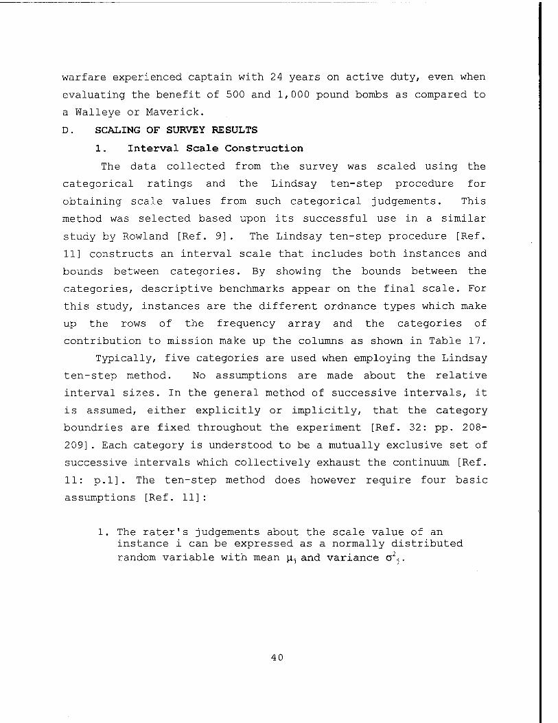
warfare experienced captain with 24 years on active duty, even when
evaluating the benefit of 500 and 1,000 pound bombs as compared to
a Walleye or Maverick.
D. SCALING OF SURVEY RESULTS
1. Interval Scale Construction
The data collected from the survey was scaled using the
categorical ratings and the Lindsay ten-step procedure for
obtaining scale values from such categorical judgements. This
method was selected based upon its successful use in a similar
study by Rowland [Ref. 9]. The Lindsay ten-step procedure [Ref.
11] constructs an interval scale that includes both instances and
bounds between categories. By showing the bounds between the
categories, descriptive benchmarks appear on the final scale. For
this study, instances are the different ordnance types which make
up the rows of the frequency array and the categories of
contribution to mission make up the columns as shown in Table 17.
Typically, five categories are used when employing the Lindsay
ten-step method. No assumptions are made about the relative
interval sizes. In the general method of successive intervals, it
is assumed, either explicitly or implicitly, that the category
boundries are fixed throughout the experiment [Ref. 32: pp. 2 08-
209]. Each category is understood to be a mutually exclusive set of
successive intervals which collectively exhaust the continuum [Ref.
11: p.l]. The ten-step method does however require four basic
assumptions [Ref. 11]:
1. The rater's judgements about the scale value of an instance i can be expressed as a normally distributed random variable with mean JU3 and variance a
2j.
40
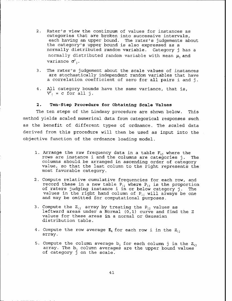
2. Rater's view the continuum of values for instances as categories that are broken into successive intervals, each having an upper bound. The rater's judgements about the category's upper bound is also expressed as a normally distributed random variable. Category j has a normally distributed random variable with mean Uj and variance o2j.
3. The rater's judgement about the scale values of instances are stochastically independent random variables that have a correlation coefficient of zero for all pairs i and j.
4. All category bounds have the same variance, that is, V2j = c for all j .
2. Ten-Step Procedure for Obtaining Scale Values
The ten steps of the Lindsay procedure are shown below. This
method yields scaled numerical data from categorical responses such
as the benefit of different types of ordnance. The scaled data
derived from this procedure will then be used as input into the
objective function of the ordnance loading model.
1. Arrange the raw frequency data in a table Fi;j where the rows are instance i and the columns are categories j. The columns should be arranged in ascending order of category value, so that the last column to the right represents the most favorable category.
2. Compute relative cumulative frequencies for each row, and record these in a new table P±j where Pi;j is the proportion of raters judging instance i in or below category j. The values in the right hand column of Pi;j will always be one and may be omitted for computational purposes.
3. Compute the ZLi array by treating the Pi;j values as leftward areas under a Normal (0,1) curve and find the Z values for these areas in a normal or Gaussian distribution table.
4. Compute the row average Z± for each row i in the ZXj array.
5. Compute the column average b-j for each column j in the ZAj array. The b-j column averages are the upper bound values of category j on the scale.
41
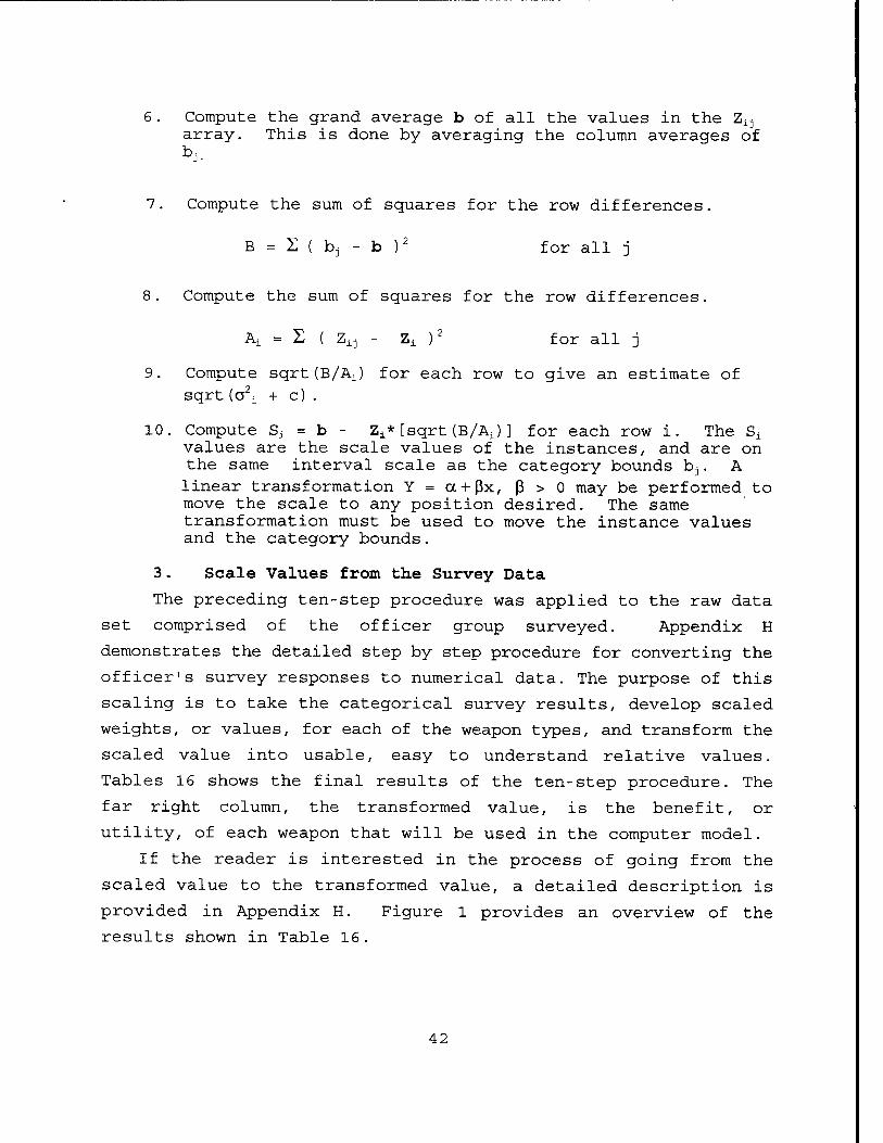
Compute the grand average b of all the values in the Z±j array. This is done by averaging the column averages of b.
7. Compute the sum of squares for the row differences.
B = I ( bj - b )2 for all j
8. Compute the sum of squares for the row differences.
Ai = I ( Zij - Z± )2 for all j
9. Compute sqrt(B/Aj for each row to give an estimate of sqrt (o2i + c) .
10. Compute Si = b - Z±* [sqrt (B/Ai) ] for each row i. The S± values are the scale values of the instances, and are on the same interval scale as the category bounds bj. A linear transformation Y = a + ßx, ß > 0 may be performed to move the scale to any position desired. The same transformation must be used to move the instance values and the category bounds.
3. Scale Values from the Survey Data
The preceding ten-step procedure was applied to the raw data
set comprised of the officer group surveyed. Appendix H
demonstrates the detailed step by step procedure for converting the
officer's survey responses to numerical data. The purpose of this
scaling is to take the categorical survey results, develop scaled
weights, or values, for each of the weapon types, and transform the
scaled value into usable, easy to understand relative values.
Tables 16 shows the final results of the ten-step procedure. The
far right column, the transformed value, is the benefit, or
utility, of each weapon that will be used in the computer model.
If the reader is interested in the process of going from the
scaled value to the transformed value, a detailed description is
provided in Appendix H. Figure 1 provides an overview of the
results shown in Table 16.
42
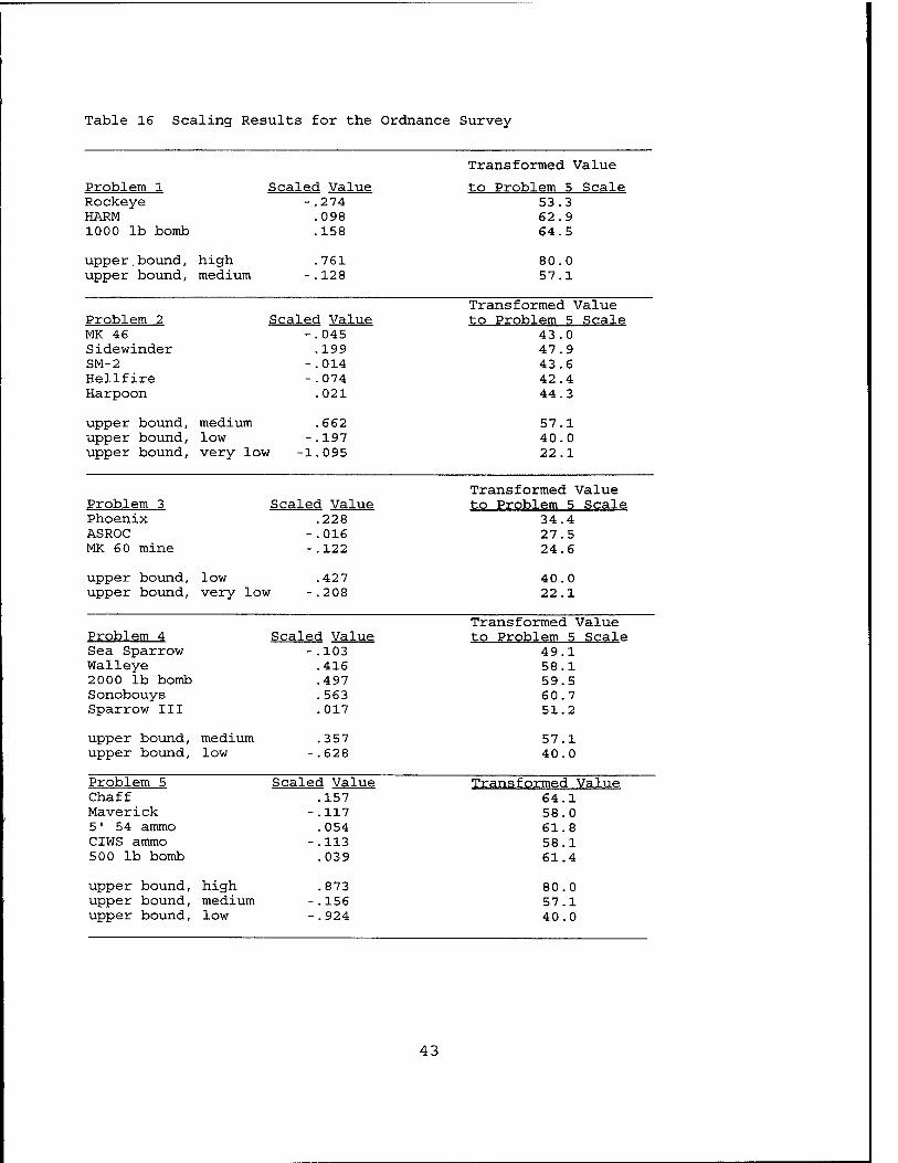
Table 16 Scaling Results for the Ordnance Survey
Transformed Value
Problem 1 Rockeye HARM 1000 lb bomb
Scaled Value -.274 .098 .158
to Problem 5 Scale 53.3 62.9 64.5
upper.bound, upper bound,
high medium
.761 -.128
80.0 57.1
Problem 2 MK 46 Sidewinder SM-2 Hellfire Harpoon
Scaled Value -.045 .199
-.014 -.074 .021
Transformed Value to Problem 5 Scale
43.0 47.9 43.6 42.4 44.3
upper bound, upper bound, upper bound,
medium .662 low -.197 very low -1.095
57.1 40.0 22.1
Problem 3 Phoenix ASROC MK 60 mine
Scaled Value .228
-.016 -.122
Transformed Value to Problem 5 Scale
34.4 27.5 24.6
upper bound, upper bound,
low very
.427 low -.208
40.0 22.1
Problem 4 Sea Sparrow Walleye 2 000 lb bomb Sonobouys Sparrow III
Scaled Value -.103 .416 .497 .563 .017
Transformed Value to Problem 5 Scale
49.1 58.1 59.5 60.7 51.2
upper bound, upper bound,
medium low
.357 -.628
57.1 40.0
Problem 5 Chaff Maverick 5' 54 ammo CIWS ammo 500 lb bomb
Scaled Value .157
-.117 .054
-.113 .039
Transformed Value 64.1 58.0 61.8 58.1 61.4
upper bound, upper bound, upper bound,
high medium low
.873 -.156 -.924
80.0 57.1 40.0
43
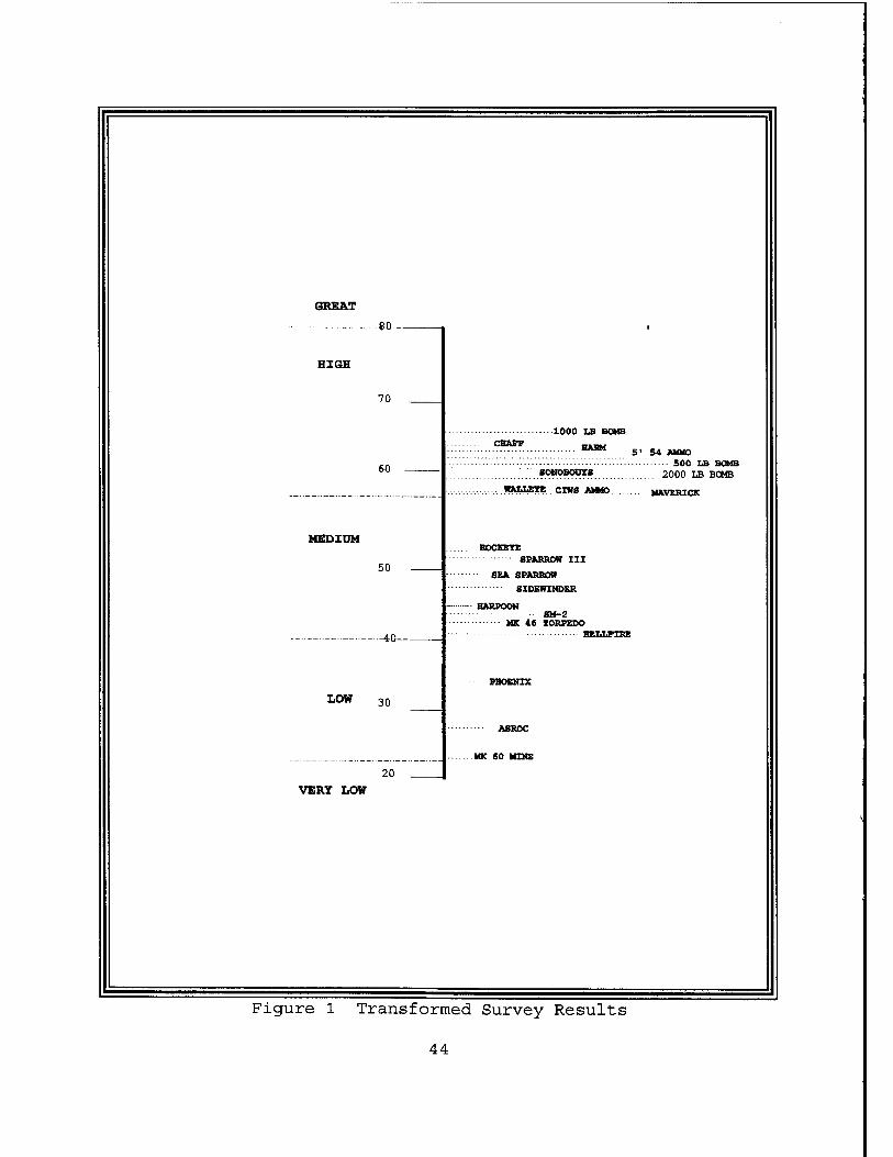
GREAT
HIGH
70
60
MEDIUM
50
-40-
LOW 30
20
1000 IS
HMM 5' 54 AMMO 500 LB BOMB
SOHOBOOYS 2000 LB BOMB
^^^v^..?•*i^^...ClW.*^•«> MAVERICK
ROCKEYE SPARROW III
SEA SPARROW SIDEWINDER
HARPOON SM—2 MK 46 TORPEDO HT.T.TJfTPT.
PHOENIX
■•• ASROC
KK SO MINE
VERY LOW
Figure 1 Transformed Survey Results
44
V. MODEL DEVELOPMENT
A. ORDNANCE LOAD MODEL
1. Methodology
The first step in developing the optimal load list model is to
decide how many weapon types are to be loaded aboard the CLF ship.
For a true AOE tailored load list, the number of different weapon
types is over 300! An example of this process for this thesis would
be the Harpoon anti-ship missile. There are currently three
versions of this missile, rail launched from a Perry class frigate,
the canister launched version, and the air launched version. Since
the escorts did not include a frigate, the rail launched Harpoon
was not included. Since the canister launched version fails the
criteria of being able to reload and fire without entering port it
was also excluded from the model. Other weapons such as 5 inch 54"
gun ammunition or Sonobouys come in many different variations. For
this model all 5 inch ammunition was lumped into one weapon type.
The modeler must also decide what benefit each weapon will bring to
the battle group. The second step is to investigate the physical
characteristics of each selected ordnance type, determine if
additional accessories would be required to employ the weapon, the
weights and volumes of each of these accessories, and the
compatibility type of each weapon. The third step is to look at the
actual size and number of ordnance storage areas on the ship to be
loaded. The fourth step is to gain an awareness for the various
constraints involved in loading ordnance aboard a ship. Factors
such as ship stability, deck stress, available storage volume and
ordnance compatibility constraints must be taken into account if
the AOE that is to be loaded correctly and safely. For this model,
steps one and two were completed in Chapter IV, while steps three
and four were completed in Chapter II.
In the final formulation, step one provides the information
for developing the sets, or indices. Steps two and three provide
45
the information that will make up the input data. Step four
provides the necessary information to be used as constraints in the
formulation equations.
2. Model Assumptions
The major assumption of this model is that all equations
relating the objective function to the constraint are linear. This
assumes that for any given quantity X, of weapon type W,
multiplied by the benefit as described in Chapter IV, is X times
more valuable to the battle group then just one weapon with the
same benefit. Other assumptions used in the design of this model
include:
1. The constraints of this linear program model consist of
volumes, weights, deck stress, ship stability and weapon storage
compatibility.
2 . As described in Chapter IV, a minimum number of each weapon
must be carried aboard the AOE. Other weapons will be loaded as
the various constraints permit.
3. There are sufficient quantities of weapons, personnel, MHE,
stowage gear and time to get the ordnance stored safely and
securely aboard the AOE. Ordnance stockpiles are sufficient to
load up to the maximum level, described in Chapter IV, of each
weapon type.
4. All ordnance loaded aboard the AOE can be transferred,
reloaded, and used, without entering port by a minimum of one ship
in the battle group.
5. The program will specify in which hold and on which deck the
ordnance item should be stowed, but not where on the deck it should
be placed (an example would be the 2nd hold, 1st Platform). Either
ship's company or the accountable Naval Weapons Station will
determine the exact storage configuration based on the model
generated load list.
6. All ordnance, including inert ordnance, will be stored in
designated ordnance storage areas aboard the ship.
46
3. Description
Indices
In this model five indices are utilized. W represents a
weapon type. For this model, the set W includes the 21 weapons as
described in Chapter IV. A second set representing the different
weapon types is also included, called WP, and is simply an alias
for W. The set AC represents a set of weapon accessories that need
to be installed on the weapons in set W to employ them in combat.
The set C represents the compatibility type that are used to
classify each weapon in set W. The final set D, represents the
number of available storage decks on the ship to be loaded.
Input Data
Input data, or parameters, list the given information with which
the model starts. The following describe each parameter in detail.
M = Large scalar number.
Volw = Each pallet or container of ordnance a combatant receives is called a unit round. This parameter shows the volume of each weapon unit round in cubic feet.
ACCVOLn
WTW
Volume of each accessory such as Harpoon wings and fins in cubic feet. While these accessories take up weight and volume on the AOE, they provide no additional benefit to the battle group, yet they must be carried if a weapon that requires an accessory is loaded.
Weight of weapon unit load in lbs divided by 1,000.
ACCWTa Weight of accessory unit load in lbs divided by 1,000.
BENEFIT w - Based upon the prioritization method described in Chapter IV, each weapon in set W received a scaled benefit value. This benefit value will be used in the objective function to optimize the AOE loadout to provide the overall highest benefit to the CVBG of all the weapons carried on the AOE.
47
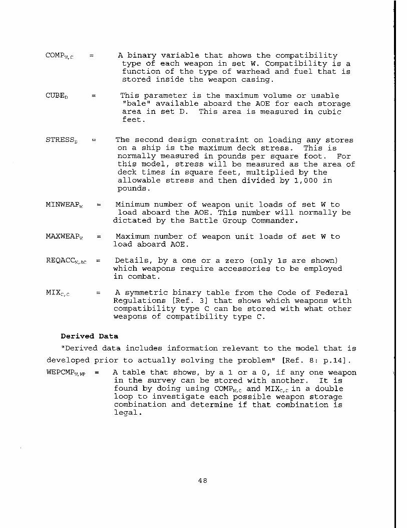
COMP w,c
CUBEr
A binary variable that shows the compatibility- type of each weapon in set W. Compatibility is a function of the type of warhead and fuel that is stored inside the weapon casing.
This parameter is the maximum volume or usable "bale" available aboard the AOE for each storage area in set D. This area is measured in cubic feet.
STRESSr
MINWEAPW
MAXWEAPW
REQACCW,AC
MIX, ■c,c
The second design constraint on loading any stores on a ship is the maximum deck stress. This is normally measured in pounds per square foot. For this model, stress will be measured as the area of deck times in square feet, multiplied by the allowable stress and then divided by 1,000 in pounds.
Minimum number of weapon unit loads of set W to load aboard the AOE. This number will normally be
dictated by the Battle Group Commander.
Maximum number of weapon unit loads of set W to load aboard AOE.
Details, by a one or a zero (only Is are shown) which weapons require accessories to be employed in combat.
A symmetric binary table from the Code of Federal Regulations [Ref. 3] that shows which weapons with compatibility type C can be stored with what other weapons of compatibility type C.
Derived Data
"Derived data includes information relevant to the model that is
developed prior to actually solving the problem" [Ref
WEPCMP - w,wp
8: p.14] .
A table that shows, by a 1 or a 0, if any one weapon in the survey can be stored with another. It is found by doing using COMPW/C and MIXC/C in a double loop to investigate each possible weapon storage combination and determine if that combination is legal.
48
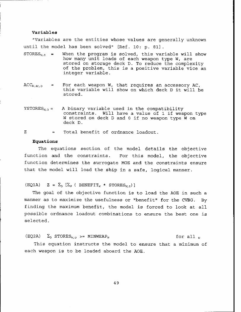
Variables
"Variables are the entities whose values are generally unknown
until the model has been solved" [Ref. 10: p. 81].
STORESWiD = When the program is solved, this variable will show how many unit loads of each weapon type W, are stored on storage deck D. To reduce the complexity of the problem, this is a positive variable vice an integer variable.
ACCW/AC/D = For each weapon W, that requires an accessory AC, this variable will show on which deck D it will be stored.
YSTORESw,D = A binary variable used in the compatibility constraints. Will have a value of 1 if weapon type W stored on deck D and 0 if no weapon type W on deck D.
Z = Total benefit of ordnance loadout.
Equations
The equations section of the model details the objective
function and the constraints. For this model, the objective
function determines the surrogate MOE and the constraints ensure
that the model will load the ship in a safe, logical manner.
(EQ1A) Z = ED [Iw ( BENEFITW * STORESw,D) ]
The goal of the objective function is to load the AOE in such a
manner as to maximize the usefulness or "benefit" for the CVBG. By
finding the maximum benefit, the model is forced to look at all
possible ordnance loadout combinations to ensure the best one is
selected.
(EQ2A) ZD STORES«, D >= MINWEAPW for all w
This equation instructs the model to ensure that a minimum of
each weapon is to be loaded aboard the AOE.
49
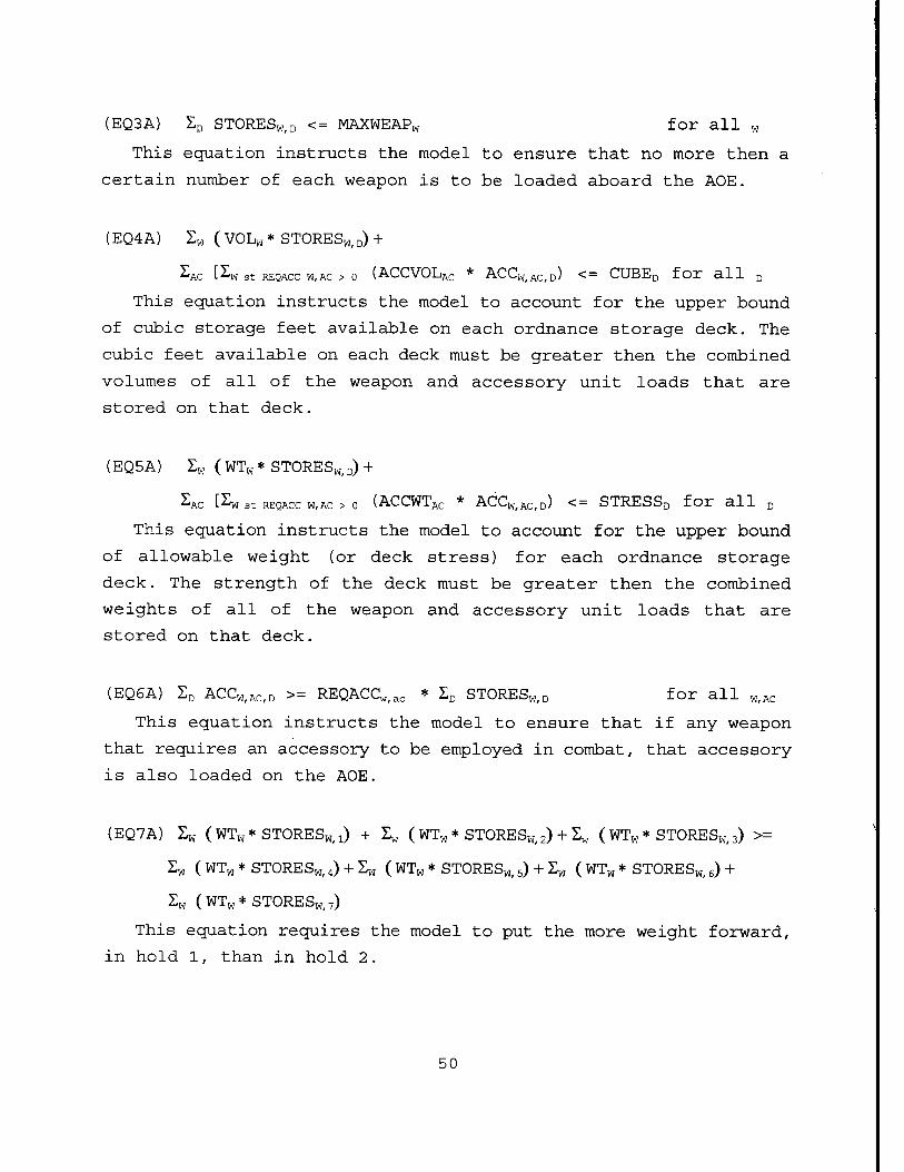
(EQ3A) SD STORES«,D <= MAXWEAPW for all w
This equation instructs the model to ensure that no more then a
certain number of each weapon is to be loaded aboard the AOE.
(EQ4A) Zw ( VOLw * STORESw, D) +
^AC [2W st REQACC W,AC > o (ACCVOLAC * ACCW,AC,D) <= CUBED for all D
This equation instructs the model to account for the upper bound
of cubic storage feet available on each ordnance storage deck. The
cubic feet available on each deck must be greater then the combined
volumes of all of the weapon and accessory unit loads that are
stored on that deck.
(EQ5A) Zw ( WTW * STORES«, D) +
^AC [^w st REQACC W,AC > o (ACCWTAC * ACCW,AC,D) <= STRESSD for all D
This equation instructs the model to account for the upper bound
of allowable weight (or deck stress) for each ordnance storage
deck. The strength of the deck must be greater then the combined
weights of all of the weapon and accessory unit loads that are
stored on that deck.
(EQ6A) ED ACCW/AC,D >= REQACCw,ac * ZD STORESW/D for all W,AC
This equation instructs the model to ensure that if any weapon
that requires an accessory to be employed in combat, that accessory
is also loaded on the AOE.
(EQ7A) Iw (WTw*STORESW/1) + Ew ( WTW * STORES„,2) + Sw ( WTW * STORESWf3) >=
E„ ( WTW * STORESw, d + £w ( WTW * STORESW/ 5) + Ew ( WTW * STORES«, 6) +
Sw (WTW* STORESw, 7)
This equation requires the model to put the more weight forward,
in hold 1, than in hold 2.
50
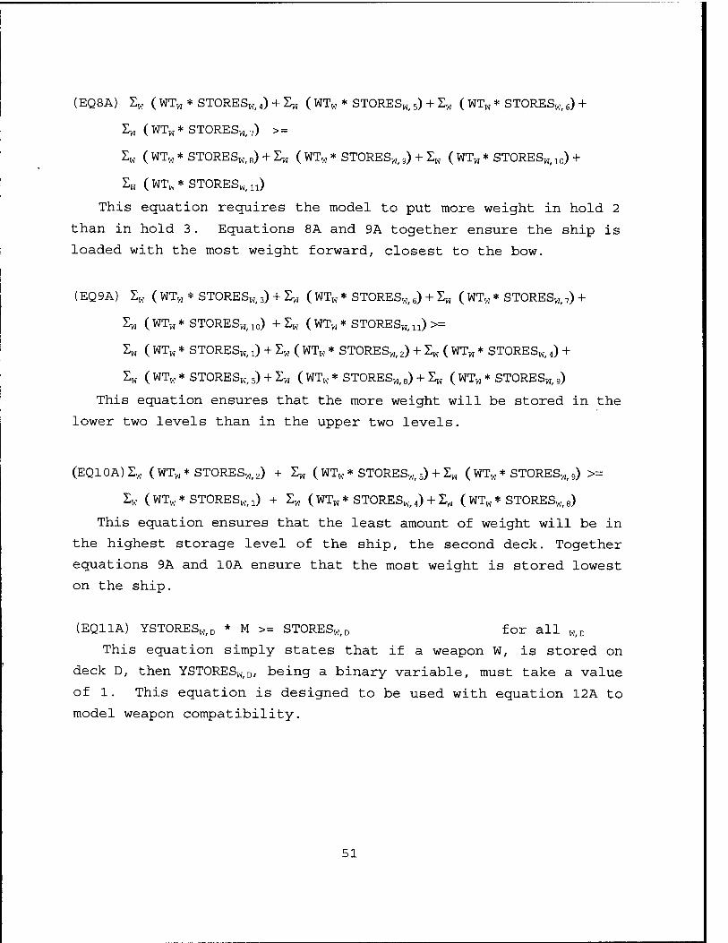
(EQ8A) E« ( WTW * STORESw, 4) + E« ( WTW * STORESW/ 5) + E« ( WTW * STORESw, 6) +
E« (WT«* STORESw,7) > =
E« ( WTW * STORESw, 8) + E„ ( WTW * STORESw, 9) + E„ ( WTW * STORES«, 10) +
E« (WT«*STORESW/11)
This equation requires the model to put more weight in hold 2
than in hold 3. Equations 8A and 9A together ensure the ship is
loaded with the most weight forward, closest to the bow.
(EQ9A) E« ( WTW * STORESw, 3) + E« ( WTW * STORES«, 6) + E« ( WTW * STORESw,7) +
E« (WTW* STORESw, 10) + ^w ( WT« * STORES«, n) >=
E« ( WTW * STORES«, 2) + E« ( WTW * STORES«, 2) + E« ( WTW * STORES«, 4) +
Ew ( WT« * STORES«, 5) + E« ( WT« * STORES«, 8) + E« ( WT« * STORES«, 9)
This equation ensures that the more weight will be stored in the
lower two levels than in the upper two levels.
(EQIOA)E« (WT«* STORES«, 2) + E« ( WT« * STORES«, 5) + E« ( WT« * STORES«, 9) >=
E„ (WT«* STORES«,a) + E« ( WT«* STORES«, 4) + E« ( WT« * STORES«, 8)
This equation ensures that the least amount of weight will be in
the highest storage level of the ship, the second deck. Together
equations 9A and 10A ensure that the most weight is stored lowest
on the ship.
(EQ11A) YSTORES«/D * M >= STORES«,D for all «,D
This equation simply states that if a weapon W, is stored on
deck D, then YSTORES„,D, being a binary variable, must take a value
of 1. This equation is designed to be used with equation 12A to
model weapon compatibility.
51
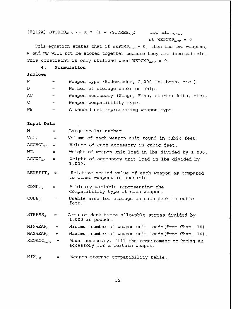
(EQ12A) STORES WP,D M * (1 YSTORES W,D^ for all W,WP,D
St WEPCMPWfMP = 0
This equation states that if WEPCMPWjWP = 0, then the two weapons,
W and WP will not be stored together because they are incompatible.
This constraint is only utilized when WEPCMPW/WP = 0.
4. Formulation
Indices
W = Weapon type (Sidewinder, 2,000 lb. bomb, etc.).
D = Number of storage decks on ship.
AC = Weapon accessory (Wings, Fins, starter kits, etc).
C = Weapon compatibility type.
WP A second set representing weapon type.
JAC —
Input Data
M
Volw
ACCVOLa
WTW
ACCWTAC
BENEFIT*
COMPw,c
CUBED
Large scalar number.
Volume of each weapon unit round in cubic feet.
Volume of each accessory in cubic feet.
Weight of weapon unit load in lbs divided by 1,000
Weight of accessory unit load in lbs divided by 1,000.
Relative scaled value of each weapon as compared to other weapons in scenario.
A binary variable representing the compatibility type of each weapon.
Usable area for storage on each deck in cubic feet.
STRESSD
MINWEAPW
MAXWEAPW
REQACCW,AC
Area of deck times allowable stress divided by 1,000 in pounds.
Minimum number of weapon unit loads(from Chap. IV)
Maximum number of weapon unit loads(from Chap. IV)
When necessary, fill the requirement to bring an accessory for a certain weapon.
MIX, c,c Weapon storage compatibility table.
52
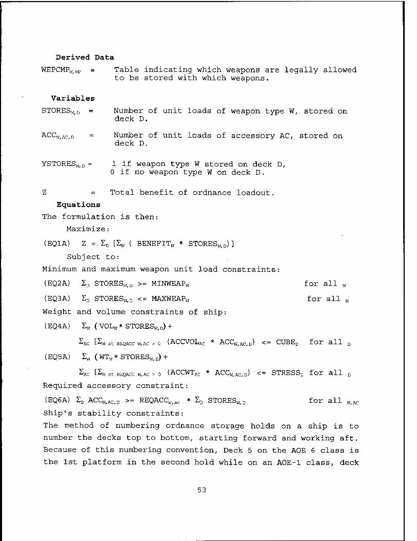
Derived Data
WEPCMPW/Wp = Table indicating which weapons are legally allowed to be stored with which weapons.
Variables
STORESW(D = Number of unit loads of weapon type W, stored on deck D.
ACCW,AC,D = Number of unit loads of accessory AC, stored on deck D.
YSTORESw,D = 1 if weapon type W stored on deck D, 0 if no weapon type W on deck D.
Z = Total benefit of ordnance loadout.
Equations
The formulation is then:
Maximize:
(EQ1A) Z = £D [Ew ( BENEFITW * STORESw,D) ]
Subject to:
Minimum and maximum weapon unit load constraints:
(EQ2A) ZD STORESWfD >= MINWEAPW for all w
(EQ3A) SD STORESW/D <= MAXWEAPW for all „
Weight and volume constraints of ship:
(EQ4A) Ew ( VOLw * STORESw, D) +
SAC [£W st REQACC W,AC > o (ACCVOLAC * ACCW,AC,D) <= CUBED for all D
(EQ5A) Ew ( WTW * STORES«, D) +
^AC [£W st REQACC W,AC > o (ACCWTAC * ACCW/AC/D) <= STRESSD for all D
Required accessory constraint:
(EQ6A) SD ACCW,AC,D >= REQACCw,ac * ED STORESW/D for all W/AC
Ship's stability constraints:
The method of numbering ordnance storage holds on a ship is to
number the decks top to bottom, starting forward and working aft.
Because of this numbering convention, Deck 5 on the AOE 6 class is
the 1st platform in the second hold while on an AOE-1 class, deck
53
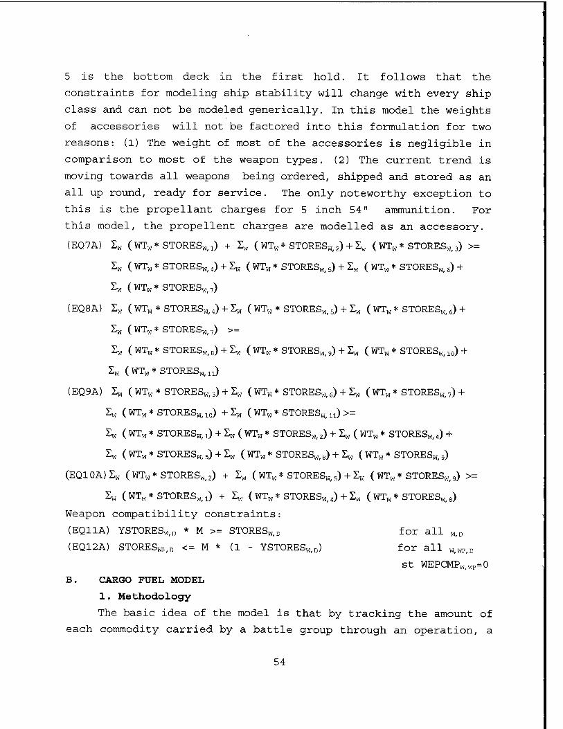
5 is the bottom deck in the first hold. It follows that the
constraints for modeling ship stability will change with every ship
class and can not be modeled generically. In this model the weights
of accessories will not be factored into this formulation for two
reasons: (1) The weight of most of the accessories is negligible in
comparison to most of the weapon types. (2) The current trend is
moving towards all weapons being ordered, shipped and stored as an
all up round, ready for service. The only noteworthy exception to
this is the propellant charges for 5 inch 54" ammunition. For
this model, the propellent charges are modelled as an accessory.
(EQ7A) Z« (WTW* STORES«, 2) + Zw ( WT« * STORES«, 2) + Zw ( WTW * STORESWf 3) >=
Z« ( WTW * STORESW/ 4) + Z« ( WTW * STORESW/ 5) + Z« ( WTW * STORESW/ 6) +
Z« (WTw*STORESW/7)
(EQ8A) Z« ( WTW * STORESw, 4) + Zw ( WTW * STORESw, 5) + Zw ( WTW * STORESw, 6) +
Z« (WTW* STORES«, 7) >=
Zw ( WTW * STORES«, 8) + Z« ( WTW * STORES«, 9) + Z« ( WT« * STORESW/10) +
Zw (WTw*STORESWfll)
(EQ9A) Z« ( WTW * STORESw, 3) + Z„ ( WT« * STORES«, 6) + Z« ( WTW * STORES»,7) +
Z« ( WTW * STORESw, 10) + Z« ( WTW * STORES«, n) >=
Z« ( WTW * STORESw, 0 + Z« ( WTW * STORES«, 2) + Z„ ( WTW * STORES», 4) +
Zw ( WTW * STORESw, 5) + Z„ ( WTW * STORESw, 8) + Zw ( WTW * STORES«, 9)
(EQ10A)ZW (WTW* STORESw, 2) + Zw ( WTW * STORESw, 5) + Z„ ( WTW * STORES«, 9) >=
Z« (WTw* STORES«, 0 + Zw (WT«* STORES«, 4) + Z« ( WT« * STORES«, 8)
Weapon compatibility constraints:
(EQ11A) YSTORES«,D * M >= STORES«,D for all W/D
(EQ12A) STORES„p,D <= M * (1 - YSTORES„,D) for all „,«p,D
st WEPCMP„,«p=0
B. CARGO FUEL MODEL
1. Methodology
The basic idea of the model is that by tracking the amount of
each commodity carried by a battle group through an operation, a
54
logistics planner would have a valuable tool to help in planning
shuttle ship requirements and schedules. By subtracting the daily
commodity usage rate from the current reserves available in the
battle group, the logistics planner can have an accurate, up to
date logistics picture. For the specific case of the Supply class
AOE, where the initial cargo fuel mix is variable, this model will
provide the logistics planner an aid to facilite finding the
optimal initial fuel loadout for the AOE-6 class station ship.
The first step in developing the model is to design a battle
group. After the composition of the battle group is known, each
combatant ship and the station ship in the battle group must be
examined individually to determine the maximum quantity of each of
the commodities that will be tracked is capable of being stored
aboard the ship. The summation of all the individual battle group
combatants, combined with the station ship cargo commodities gives
the maximum amount of each commodity available for the battle
group. With the AOE-6 assigned as a station ship, the JP-5 and DFM
commodities have a maximum initial range.
The next step is to again return to each individual ship in
the battle group and find the individual ship consumption rates
during the various phases of the operation for each commodity.
Again, the summation of the individual ship usage rates for each
of the commodities during each phase of the operation provides the
daily battle group usage rate. For this model, the previous steps
were completed in Chapter III.
In the final formulation, the commodities to be tracked and
the length of the operation, in days, provide the information for
developing the sets. The rest of the information is used to make
up the input data.
The interesting aspect of this model is that while the overall
MOE is to minimize the number of CONSOLS required during the
operation, the objective function in the optimization formulation
is to maximize the quantity of commodities that are transferred to
the CVBG. The objective function performs the task of ensuring
that for every CONSOL operation, the CVBG will attempt to replenish
55
to its initial values. To find the correct or minimum, number of
CONSOLS to perform, a constraint equation will be employed with the
number of CONSOL operations during the model run equal to a
positive integer. This will require the user to set in a specific
number that will be equal to the number of CONSOL operations
throughout the operation. The user will then modify the number of
CONSOL operations, over several model run iterations until the
smallest number of CONSOL operations that provide a feasible
solution can be found. For this model a feasible solution is a
solution which maintains the battle group above the pre-determined
reserve level for each commodity in the battle group throughout the
80 day operation.
The first approach to this model attempted to have an
objective function that minimized the number of CONSOLS during the
operation. The problem with this approach is that the initial load
of cargo fuel for the AOE is a variable, so it is not possible to
force the model to fully load every commodity to its initial levels
at every CONSOL without using non-linear programming techniques.
2. Model Assumptions
Several assumptions were made to simplify the model. The most
important assumption is that all commodities used by the battle
group are aggregated and expended through the AOE, rather then by
the individual units. This is done by expanding the capacity of
the AOE to include the entire battle group. The advantage of this
is the effect of eliminating the need to model specific underway
replenishments to the combatants in the battle group. It also
allows the user to set a minimum commodity level for the battle
group as a whole, vice a minimum for each individual ship.
Other assumptions include:
1. One AOE is assigned to the battle group as a station ship.
Sufficient shuttle ships are available to fully resupply each
commodity to the initial (maximum) level at any time before one
commodity drops to its minimum level. Factors such as turnaround
time and distance from the ALSS will not be considered in this
model.
56
2. Internal distribution from the AOE to the battle group occurs,
but is transparent.
3. While 30% of the AOE-6 cargo fuel tanks are convertible, no
other storage spaces may be used to store any other cargo than
specifically assigned (for example, no placing ordnance in dry
goods storage holds). The common fleet practice of deck loading
dry stores and inert ordnance will also not be modelled.
4. The battle group will begin each scenario at the maximum level
for all commodities.
3. Description
Indices
This model involves only two indices. The first indice is I,
which represents the set of the four commodities, DFM, JP5, STORES
and AMMO, that will be tracked in the model. The second indice T,
represents the day of the operation, in this case day 1 through day
80.
Input Data
MINLEVEL! =
MAXLEVELT =
USED I,T
This is the minimum battle group reserve level for each commodity. This reserve level is normally set by the fleet or battle group commander. It is usually measured as a percentage of the maximum commodity storage level.
This represents the maximum storage capacity in the battle group for each commodity. This is based upon the storage constraints of the ships in the battle group.
A table that represents the daily usage rates for each commodity for each day of the peration. Because of the large size of this table, it is entered as a separate file. The daily usage rates are dependent on which phase of the operation and the composition of the CVBG.
N A scalar number that tells the model the exact number of CONSOL operations to perform during the operation. This number will start high and on each run be made smaller until the model can no longer find a feasible solution. This has the effect of finding the minimum number of CONSOLS based upon the CVBG composition and required minimum reserve levels.
57
Variables
A0E6I/T
CONSOL I,T
INITAOET =
DAYT
OBJECT
This variable represents the reserve quantity of each commodity, I, available to the battle group at the completion of each day, T.
Tracks the quantity of each commodity that was CONSOLed to the CVBG on each day.
This is the variable that will tell the optimal mix of cargo fuel to carry. This is accomplished by setting a high and low range for the maximum CVBG fuel capacity which reflects the alignment of the AOE having all of its convertible tanks to DFM of all to JP5. The STORES and AMMO commodities are fixed at the maximum capacity for the ship.
A binary decision variable of whether or not to CONSOL on day T. If a 1, then the CVBG will conduct a CONSOL operation.
While minimizing the number of CONSOL operations, maximize the quantity of each commodity CONSOLed to the CVBG.
Equations
(EQ1B) OBJECT [ET CONSOL!/T ]
The goal of the objective function is to maximize the quantity
of each commodity transferred to the battle group. This forces the
model to efficiently plan each of the limited number of CONSOLS to
ensure maximum efficiency.
(EQ2B) ZT DAYT = N
This equation is where the number of CONSOL evolutions permitted
during the entire operation is controlled.
(EQ3B) A0E6IfT = INITAOE! - USEDI/T + CONSOLI/T for all I>T=1
This equation shows the reserve level of each commodity at the
end of day 1. This equation is necessary because the initial
loadout of the AOE is a variable. While it is highly unlikely that
the CVBG would need to CONSOL on its first day out of port, the
computer model attempts to do so if the CONSOLIfT were not added to
this equation.
58
(EQ4B) A0E6I/T = AOEG^T.! - USEDI/T + CONSOLIrT for all IrT>1
This equation is the flow balance equation for each of the
commodities from day 2 to the end of the operation.
(EQ5B) A0E6IfT >= MINLEVEI^ for all :
This equation sets the minimum reserve level for each
commodity in the CVBG. When any one of the four commodities
reaches its minimum level a CONSOL must take place to resupply the
battle group.
(EQ6B) A0E6lfT <= INITAOE: for all x
This equation states that once the initial AOE loadout has been
determined, those capacities now become the upper bounds and the
battle group may never carry more then that quantity of each
commodity. This, in concert with equation 7B, also sets the upper
limit on how much of each commodity may be CONSOLed.
(EQ7B) CONSOL:,T <= MAXLEVELx * DAYT for all IfT
This equation is where the YES or NO decision to CONSOL on day
T occurs. If the decision is NO, then CONSOLI/T = 0, if the
decision is YES, then equation IB attempts to CONSOL as much as
possible, while this equation and equation 6B provide the upper
bound constraint.
(EQ8B) 2r INITAOEx = 13,156,901 * .95 for I= JP5,Dm
This equation tells the model that the sum of the initial JP-5
and DFM fuel load, in gallons, is equal to the maximum fuel
capacity for the battle group. INITAOE is given an upper and a
lower bound for the commodities DFM and JP-5 in the model. This
range is based on the convertible tank storage capacity aboard the
AOE-6 class. The quantity, .95, is the stow factor for the fuel
tanks in the battle group.
(EQ9B) INITAOE! = 1,658.42 for I= ST0RES
(EQ10B) INITAOEj = 5,016 for ^ „„,
59
Based upon the unclassified ordnance and stores capacities for
each ship in the battle group, equation 9B and 10B tell the model
to have a maximum initial loadout of these two commodities. The
final three equations are utilized only if modeling a ship that has
a variable initial maximum load such as the AOE-6 class. A stowage
factor was not applied to the final two equations. The reason for
this is that the ship weapon loads were taken from a notional load
list. The weapons, like the stores, are already aboard the ship,
so a stow factor is not required. For the cargo stores and
ordnance, the ship design contractor's expected loadout, by weight
(tons), was used as a planning factor. Stow factors affect volume,
not weight, so again this factor was dropped. If the station ship
in the scenario was an AOE-1 class, the INITAOE variable would not
be required, and the initial loadout would be equal to the maximum
loadout.
4. Formulation
Indices
I = Commodity type.
T = Day of the operation.
Input Data
MINLEVELj = Min CVBG reserve (on-hand) level of commodity I.
MAXLEVEL! = Max CVBG level of commodity I.
USEDIiT = Quantity of commodity I consumed on day T.
N A scalar equal to the number of CONSOL operations.
Variables
A0E6IfT = CVBG reserve level of commodity I on day T.
CONSOLI/T = Amount of commodity I consoled on day T.
INITAOE! = Initial (and maximum) quantity of commodity I.
DAYT = Yes or no decision to CONSOL on day T.
OBJECT = Minimize number of CONSOLS and refill to capacity.
Equations
The formulation is then:
Maximize:
(EQ1B) OBJECT = Zj [ZT CONSOLI/T ]
60
Subject to:
Find the minimum number of CONSOLS:
(EQ2B) IT DAYT = N
The flow balance equations:
(EQ3B) A0E6IfT = INITAOEj - USEDI(T + CONSOLI/T for all IfT_x
(EQ4B) A0E6IfT = AOEÖ!,^! - USEDI/T + CONSOLIfT for all I/T>1
Observe minimum reserve levels:
(EQ5B) A0E6IfT >= MINLEVE^ for all x
Observe storage capacities:
(EQ6B) A0E6IfT <= INITAOEj for all 2
Did a CONSOL occur on a given day:
(EQ7B) CONSOLIfT <= MAXLEVELj * DAYT for all I/T
The initial fuel load on the AOE:
(EQ8B) Ij INITAOEj = 13,156,901 * .95 for I= JP5,Dm
The initial stores and ordnance load:
(EQ9B) INITAOEj = 1,658.42 for i= STORES
(EQ10B) INITAOE! = 5,016 for I= ^o
C. GENERAL ALGEBRAIC MODEL SYSTEM
The General Algebraic Modeling System, or GAMS, is used to
solve both models. "GAMS is designed to make the construction and
solution of large and complex mathematical programming models more
straightforward for programmers and more comprehensible to users of
models from other disciplines" [Ref. 10: Preface]. In the first
model, GAMS is used to find the maximum benefit of the entire
ordnance load aboard the AOE. In the second model, GAMS will be
used to find the optimal initial DFM to JP-5 cargo fuel mix to
carry on the AOE.
Mixed integer programs, like these two models, are generally
difficult to solve and often require extensive computing resources.
GAMS provides an option for relative and absolute termination
tolerances (OPTCR and OPTCA) which can be defined by the user,
allowing GAMS to stop when the objective function value is within
61
a certain tolerance of the optimal solution. Both models will use
termination boundaries of five percent to aid in determining a
final solution.
62
VI. SUMMARY OF RESULTS AND CONCLUSIONS
A. ORDNANCE LOAD MODEL RESULTS
This GAMS program models the loading of ordnance aboard a
Supply class AOE. The measure of effectiveness for this model is
the overall benefit of the ordnance loadout to a carrier battle
group. For the AOE-6 loadout, the objective function value was
109,972.8734. Unfortunately, this program has only been developed
and executed for one class of ship, so the objective function value
has no other results with which to compare and develop conclusions.
One alternative scale of measurement is to look at the total number
of each weapon type loaded aboard the AOE-6. Of the 21 weapon
types used in the model, the program loaded 13 weapon types to the
maximum allowable level, six at the minimum level and two at levels
between the minimum and maximum. Table 17 shows the number of each
weapon loaded aboard the AOE-6. Appendix I contains the complete
output file showing which deck to store each of the weapons as
well as the necessary accessories.
63
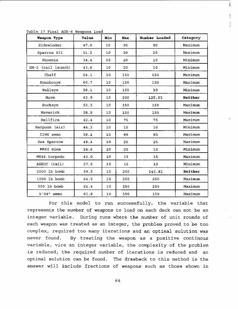
Table 17 Final AOE-6 Weapons Load
Weapon Type Value Min Max Number Loaded Category
Sidewinder 47.9 10 90 90 Maximum
Sparrow III 51.2 10 20 20 Maximum
Phoenix 34.4 10 20 10 Minimum
SM-2 (rail launch) 43.6 10 20 10 Minimum
Chaff 64.1 10 150 150 Maximum
Sonobouys 60.7 10 150 150 Maximum
Walleye 58.1 10 150 10 Minimum
Harm 62.9 10 200 125.53 Neither
Rockeye 53.3 10 150 150 Maximum
Maverick 58.0 10 150 150 Maximum
Hellfire 42.4 10 75 75 Maximum
Harpoon (air) 44.3 10 15 10 Minimum
CIWS ammo 58.1 10 80 80 Maximum
Sea Sparrow 49.1 10 25 25 Maximum
MK60 mine 24.6 10 25 10 Minimum
MK46 torpedo 43.0 10 15 15 Maximum
ASROC (rail) 27.5 10 15 10 Minimum
2000 lb bomb 59.5 10 250 143.81 Neither
1000 lb bomb 64.5 10 250 250 Maximum
500 lb bomb 61.4 10 250 250 Maximum
5'54" ammo 61.8 10 150 150 Maximum
For this model to run successfully, the variable that
represents the number of weapons to load on each deck can not be an
integer variable. During runs where the number of unit rounds of
each weapon was treated as an integer, the problem proved to be too
complex, required too many iterations and an optimal solution was
never found. By treating the weapon as a positive continous
variable, vice an integer variable, the complexity of the problem
is reduced, the required number of iterations is reduced and an
optimal solution can be found. The drawback to this method is the
answer will include fractions of weapons such as those shown in
64
Table 19 for the two "Neither" category weapons. A review of the
output file shown in Appendix I will also reveal this drawback for
some of the weapons and accessories that are stored on several
decks, with fractions of weapon loads on each deck. In these
cases, the experience of the load planner and ship's company will
dictate which course of action to take. In the case of the AOE-6,
the limiting factor is the lack of available weapons storage area.
For this case, the fraction portion of the weapon will probably be
rounded down to the next lower whole unit load.
Another yardstick of the worth of the ordnance onload is the
total tonnage of ordnance the GAMS program was able to place aboard
the AOE. For the data parameters as shown in Appendix I, the total
ordnance tonnage was 2,354. The ship design specifications
anticipate the required ordnance load for this class of ship to be
1,800 tons. This large discrepancy is a result of the limited
selection of weapon types loaded aboard the AOE for this model. The
weapons loaded in this program were all larger, heavier types of
ordnance. When the loadout includes lighter, smaller or less
efficiently stored ordnance such as blasting caps, detonation chord
or small arms ammunition, the result will be a lower overall
tonnage of the ordnance loadout.
The issue of compatibility also did not play a major role in
the program results. While the Harpoon missile did test the
model's compatibility constraints, should the loadout include other
ordnance types that require special handling, such as star shells
(pyrotechnics), possibly special weapons or phosphorous 5 inch 54"
rounds, the compatibility constraint would play a much larger role
in the final load list and would also probably lower the total
loadout tonnage.
The important structural design feature of the AOE-6 class,
brought to light by the results, is that even though the total
ordnance tonnage was greater than the contractors anticipated
tonnage, the loadout did not come within 60% of the rated stress
65
load for any of the storage decks. This significant detail allows
for the free use of forktrucks in the ammunition holds to move
ordnance, without the fear of over stressing the deck.
B. CARGO FUEL MODEL RESULTS
When reviewing the results of the Battle Group Commodity Level
Program, it is very important for the reader to understand that the
results are relative to the data used in the program. While every
effort has been made to model the commodity usage for a battle
group involved in a real world contingency, several items must be
mentioned to ensure the reader fully understands the limitations of
this thesis program.
The figures used to arrive at the maximum fuel capacities of
DFM and JP-5 for the battle group are all taken from unclassified
sources.
The ordnance expenditure rate can fluctuate up or down
depending upon the type of weapons being employed. If the mission
requires a larger number of advanced, smart weapons, the ordnance
usage may drop. Ordnance usage is also dependent on the threat to
the battle group from air, surface and submarine contacts. No
surface ships fired anti-air or anti-surface missiles, or torpedoes
during the Persian Gulf War. Should a scenario develop against a
foe with a formidable AAW, ASUW or ASW threat, the usage rates may
be higher.
The JP-5 daily usage rate is dependent on the number of
sorties flown. A fleet logistics planner would have to evaluate
the strike mission requirements as well as the defensive posture of
the battle group to arrive at his final JP-5 usage rates.
For this program, the minimum reserve level of any commodity
will be set at 70%. The minimum level of the cargo fuel is based
on the minimum possible JP-5 or DFM loadout (to find the 70% DFM
level, assume all convertible tanks are carrying JP-5, total the
remaining DFM in the battle group and multiply by .7) . Sensitivity
analysis discussed later in this chapter will look at the impact of
lowering this level, but fleet experience indicates a preference to
have a minimum on-hand availability of at least 70%. The first run
66
for each scenario will look at finding the optimal fuel mix and the
minimum number of CONSOLS. Two more model runs will be completed
by loading the convertible tanks aboard the AOE-6 with all JP-5 and
then all DFM. The goal is that at the end of all four scenarios,
a cargo fuel mix will be found that when placed in all four
scenarios will come as close as possible to replicating the minimum
number of CONSOLS for each of the individual scenarios as the
generated optimal fuel mix. This will find the best cargo tank
configuration for an AOE-6 to respond to all taskings without
having to empty and convert fuel tanks.
The results of the model runs were slightly different than
anticipated. What the model would do, instead of totally reloading
the battle group to 100% at each CONSOL for each commodity, is
resupply each commodity at such a level as to just make it through
to the next CONSOL, until the last CONSOL of the operation where it
would proceed to load to 100% for every commodity. By conducting
CONSOLS in this manner, it still managed to maximize the objective
function, still managed to minimize the number of CONSOLS, it just
did not act in a way that a fleet logistics planner would. While it
did not do this more then 35% of the time, it required a more
detailed analysis of the results to discover which commodity was
the limiting factor. The difference between the model and the
human planner is the model is strictly looking to optimize the
allocation of CONSOLS to gain a maximum benefit, while the human
planner would be taking other factors such as operations,
availability of shuttle ships and the threat level into account
when planning CONSOLS. The main focus is looking at which
commodities were the limiting factors for the battle group and what
is the recommended split of cargo fuel for the AOE-6 class station
ship to carry.
1. Nuclear Powered CV and Escorts (Scenario 1)
The model required a total of seven CONSOLS for the 80 day
operation. Two CONSOLS occurred during the transit phase, both
motivated by the DFM level, two CONSOLS occurred during the
presence, both due to JP-5 reaching the minimum level, and the
67
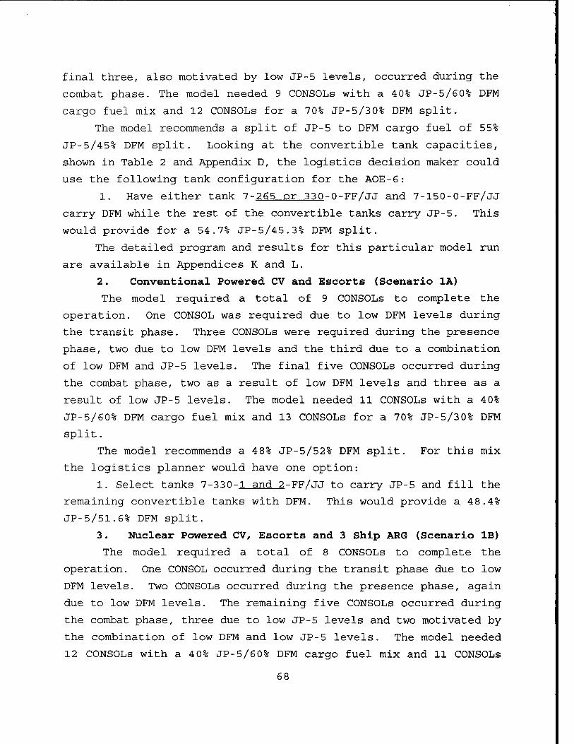
final three, also motivated by low JP-5 levels, occurred during the
combat phase. The model needed 9 CONSOLS with a 40% JP-5/60% DFM
cargo fuel mix and 12 CONSOLS for a 70% JP-5/30% DFM split.
The model recommends a split of JP-5 to DFM cargo fuel of 55%
JP-5/45% DFM split. Looking at the convertible tank capacities,
shown in Table 2 and Appendix D, the logistics decision maker could
use the following tank configuration for the AOE-6:
1. Have either tank 7-265 or 330-0-FF/JJ and 7-150-0-FF/JJ
carry DFM while the rest of the convertible tanks carry JP-5. This
would provide for a 54.7% JP-5/45.3% DFM split.
The detailed program and results for this particular model run
are available in Appendices K and L.
2. Conventional Powered CV and Escorts (Scenario 1A)
The model required a total of 9 CONSOLS to complete the
operation. One CONSOL was required due to low DFM levels during
the transit phase. Three CONSOLS were required during the presence
phase, two due to low DFM levels and the third due to a combination
of low DFM and JP-5 levels. The final five CONSOLS occurred during
the combat phase, two as a result of low DFM levels and three as a
result of low JP-5 levels. The model needed 11 CONSOLS with a 40%
JP-5/60% DFM cargo fuel mix and 13 CONSOLS for a 70% JP-5/30% DFM
split.
The model recommends a 48% JP-5/52% DFM split. For this mix
the logistics planner would have one option:
1. Select tanks 7-330-1 and 2-FF/JJ to carry JP-5 and fill the
remaining convertible tanks with DFM. This would provide a 48.4%
JP-5/51.6% DFM split.
3. Nuclear Powered CV, Escorts and 3 Ship ARG (Scenario IB)
The model required a total of 8 CONSOLS to complete the
operation. One CONSOL occurred during the transit phase due to low
DFM levels. Two CONSOLS occurred during the presence phase, again
due to low DFM levels. The remaining five CONSOLS occurred during
the combat phase, three due to low JP-5 levels and two motivated by
the combination of low DFM and low JP-5 levels. The model needed
12 CONSOLS with a 40% JP-5/60% DFM cargo fuel mix and 11 CONSOLS
68
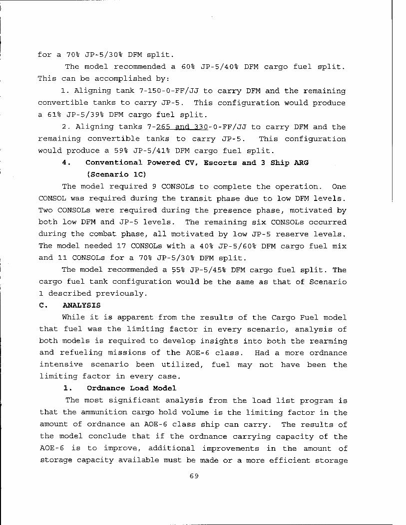
for a 70% JP-5/30% DFM split.
The model recommended a 60% JP-5/40% DFM cargo fuel split.
This can be accomplished by:
1. Aligning tank 7-150-0-FF/JJ to carry DFM and the remaining
convertible tanks to carry JP-5. This configuration would produce
a 61% JP-5/39% DFM cargo fuel split.
2. Aligning tanks 7-265 and 330-0-FF/JJ to carry DFM and the
remaining convertible tanks to carry JP-5. This configuration
would produce a 59% JP-5/41% DFM cargo fuel split.
4. Conventional Powered CV, Escorts and 3 Ship ARG
(Scenario 1C)
The model required 9 CONSOLS to complete the operation. One
CONSOL was required during the transit phase due to low DFM levels.
Two CONSOLS were required during the presence phase, motivated by
both low DFM and JP-5 levels. The remaining six CONSOLS occurred
during the combat phase, all motivated by low JP-5 reserve levels.
The model needed 17 CONSOLS with a 40% JP-5/60% DFM cargo fuel mix
and 11 CONSOLS for a 70% JP-5/30% DFM split.
The model recommended a 55% JP-5/45% DFM cargo fuel split. The
cargo fuel tank configuration would be the same as that of Scenario
1 described previously.
C. ANALYSIS
While it is apparent from the results of the Cargo Fuel model
that fuel was the limiting factor in every scenario, analysis of
both models is required to develop insights into both the rearming
and refueling missions of the AOE-6 class. Had a more ordnance
intensive scenario been utilized, fuel may not have been the
limiting factor in every case.
1. Ordnance Load Model
The most significant analysis from the load list program is
that the ammunition cargo hold volume is the limiting factor in the
amount of ordnance an AOE-6 class ship can carry. The results of
the model conclude that if the ordnance carrying capacity of the
AOE-6 is to improve, additional improvements in the amount of
storage capacity available must be made or a more efficient storage
69
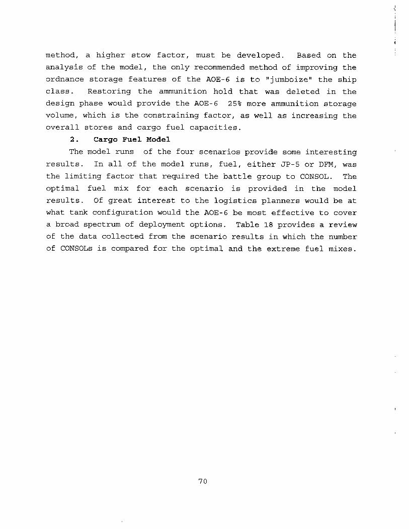
method, a higher stow factor, must be developed. Based on the
analysis of the model, the only recommended method of improving the
ordnance storage features of the AOE-6 is to "jumboize" the ship
class. Restoring the ammunition hold that was deleted in the
design phase would provide the AOE-6 25% more ammunition storage
volume, which is the constraining factor, as well as increasing the
overall stores and cargo fuel capacities.
2. Cargo Fuel Model
The model runs of the four scenarios provide some interesting
results. In all of the model runs, fuel, either JP-5 or DFM, was
the limiting factor that required the battle group to CONSOL. The
optimal fuel mix for each scenario is provided in the model
results. Of great interest to the logistics planners would be at
what tank configuration would the AOE-6 be most effective to cover
a broad spectrum of deployment options. Table 18 provides a review
of the data collected from the scenario results in which the number
of CONSOLS is compared for the optimal and the extreme fuel mixes.
70
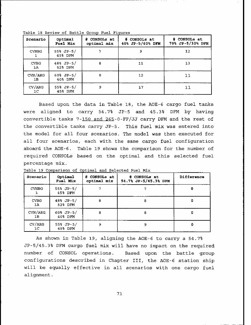
Table 18 Review of Battl e Group Fuel Figures
Scenario Optimal Fuel Mix
# CONSOLS at optimal mix
# CONSOLS at 40% JP-5/60% DFM
# CONSOLS at 70% JP-5/30% DFM
CVNBG 1
55% JP-5/ 45% DFM
7 9 12
CVBG 1A
48% JP-5/ 52% DFM
8 11 13
CVN/ARG IB
60% JP-5/ 40% DFM
8 12 11
CV/ARG 1C
55% JP-5/ 45% DFM
9 17 11
Based upon the data in Table 18, the AOE-6 cargo fuel tanks
were aligned to carry 54.7% JP-5 and 45.3% DFM by having
convertible tanks 7-150 and 265-0-FF/JJ carry DFM and the rest of
the convertible tanks carry JP-5. This fuel mix was entered into
the model for all four scenarios. The model was then executed for
all four scenarios, each with the same cargo fuel configuration
aboard the AOE-6. Table 19 shows the comparison for the number of
required CONSOLS based on the optimal and this selected fuel
percentage mix.
Table 19 Comparison of Optimal and Selected Fuel Mix
Scenario Optimal Fuel Mix
# CONSOLS at optimal mix
# CONSOLS at 54.7% JP-5/45.3% DFM
Difference
CVNBG 1
55% JP-5/ 45% DFM
7 7 0
CVBG 1A
48% JP-5/ 52% DFM
8 8 0
CVN/ARG IB
60% JP-5/ 40% DFM
8 8 0
CV/ARG 1C
55% JP-5/ 45% DFM
9 9 0
As shown in Table 19, aligning the AOE-6 to carry a 54.7%
JP-5/45.3% DFM cargo fuel mix will have no impact on the required
number of CONSOL operations. Based upon the battle group
configurations described in Chapter III, the AOE-6 station ship
will be equally effective in all scenarios with one cargo fuel
alignment.
71
D. SENSITIVITY ANALYSIS
1. Ordnance Load Model
From the results produced in the ordnance loading model, it is
clear that two parameters affect the final generated load list; the
benefit and the volume of each weapon. Attempts to influence the
final results by modifying the weight of the weapons or the
stability constraints yielded no changes. The benefit of each
weapon was taken from the Chapter IV survey results and is employed
in the objective function. The benefit of each weapon was derived
from a comparison with other weapons in a group. To arbitrarily
change any one weapon's worth as compared to the other weapons in
the group is not realistic, so only the volume of the unit round of
each weapon will be explored.
For this analysis, two additional ordnance loads will be
completed. The first will look at a 10% volume increase for each
of the 21 weapon types. The rationale for this is that as the
military moves more towards issuing weapons with all the required
accessories, or as an All-Up-Round (AUR), the size of the unit load
will increase. The second will look at a 10% decrease in the size
of the 21 weapon types. The thought here is that as technology can
produce better fuels, more powerful warheads and better guidance
systems, the size of weapons may actually decrease. Again, the
purpose is to see the effect of these volume changes on the final
ordnance loadout. Table 2 0 shows the results of this sensitivity
analysis.
72
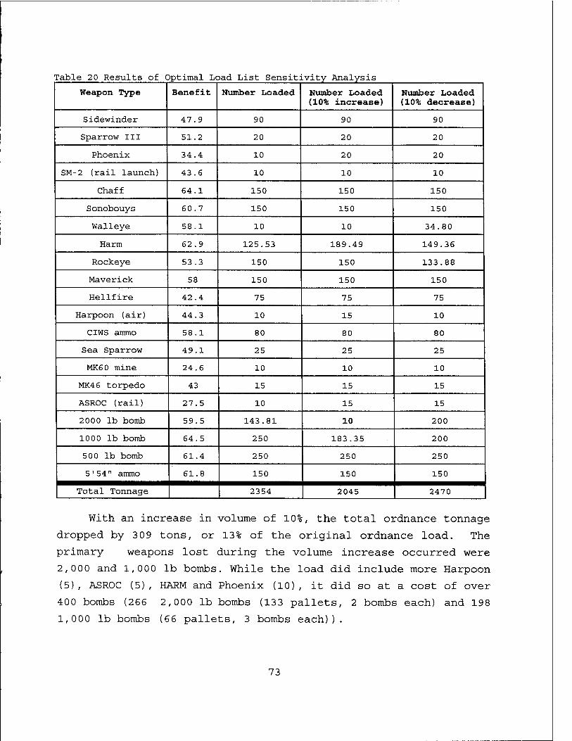
Table 2 0 Results of Optimal Load List Sensitivity Analysis
Weapon Type Benefit Number Loaded Number Loaded (10% increase)
Number Loaded (10% decrease)
Sidewinder 47.9 90 90 90
Sparrow III 51.2 20 20 20
Phoenix 34.4 10 20 20
SM-2 (rail launch) 43.6 10 10 10
Chaff 64.1 150 150 150
Sonobouys 60.7 150 150 150
Walleye 58.1 10 10 34.80
Harm 62.9 125.53 189.49 149.36
Rockeye 53.3 150 150 133.88
Maverick 58 150 150 150
Hellfire 42.4 75 75 75
Harpoon (air) 44.3 10 15 10
CIWS ammo 58.1 80 80 80
Sea Sparrow 49.1 25 25 25
MK60 mine 24.6 10 10 10
MK46 torpedo 43 15 15 15
ASROC (rail) 27.5 10 15 15
2000 lb bomb 59.5 143.81 10 200
1000 lb bomb 64.5 250 183.35 200
500 lb bomb 61.4 250 250 250
5'54" ammo 61.8 150 150 150
Total Tonnage 2354 2045 2470
With an increase in volume of 10%, the total ordnance tonnage
dropped by 3 09 tons, or 13% of the original ordnance load. The
primary weapons lost during the volume increase occurred were
2,000 and 1,000 lb bombs. While the load did include more Harpoon
(5), ASROC (5), HARM and Phoenix (10), it did so at a cost of over
400 bombs (266 2,000 lb bombs (133 pallets, 2 bombs each) and 198
1,000 lb bombs (66 pallets, 3 bombs each)).
73
The decrease in volume of 10% added only an additional 116
tons, or 5% to the original load. The weapons that decreased in
the final load were 1,000 lb bombs (50 pallets or 150 total bombs)
and Rockeye (16), but the final load included 56 more pallets of
2,000 lb bombs (112 bombs), more ASROC (5), HARM (24), and Walleye
(24) .
Again, this model loads ordnance as dimensionless objects.
This allows the model to perfectly fit each container and pallet
with no gaps. When loading actual squares, rectangles and boxes,
the fit may not be as tight, hence the need for dunnage and
bracing. It is obvious from this model that with the advanced
structural design and strength of the ammunition holds aboard the
AOE-6 class, the available storage volume will continue to be the
primary constraint. This sensitivity implies that the AOE-6 will
be much more affected by increases in weapon volume then by
decreases. The real world loading of ammunition may not be as
adversely impacted by the 10% weapon volume increase as was the
model, but an increase will have a much more pronounced impact on
the final load list then a 10% decrease in the volume.
2. Cargo Fuel Model
a. Impact of Lowering the Minimum Commodity Reserve Levels
With a limited number of shuttle ships that can be
deployed at any given moment, just how long can an AOE keep a CVBG
fueled, armed and supplied? What if the contingency developed in
a place where the Navy did not have a regular supply pipeline, yet
the carrier and her escorts were required to go? To look at these
questions, the reserve commodity levels were dropped from 70% to
3 0% in increments of 10% to see the impact on the recommended
optimal fuel mix, as well as the required number of CONSOLS. Table
21 shows the results of the model runs.
74
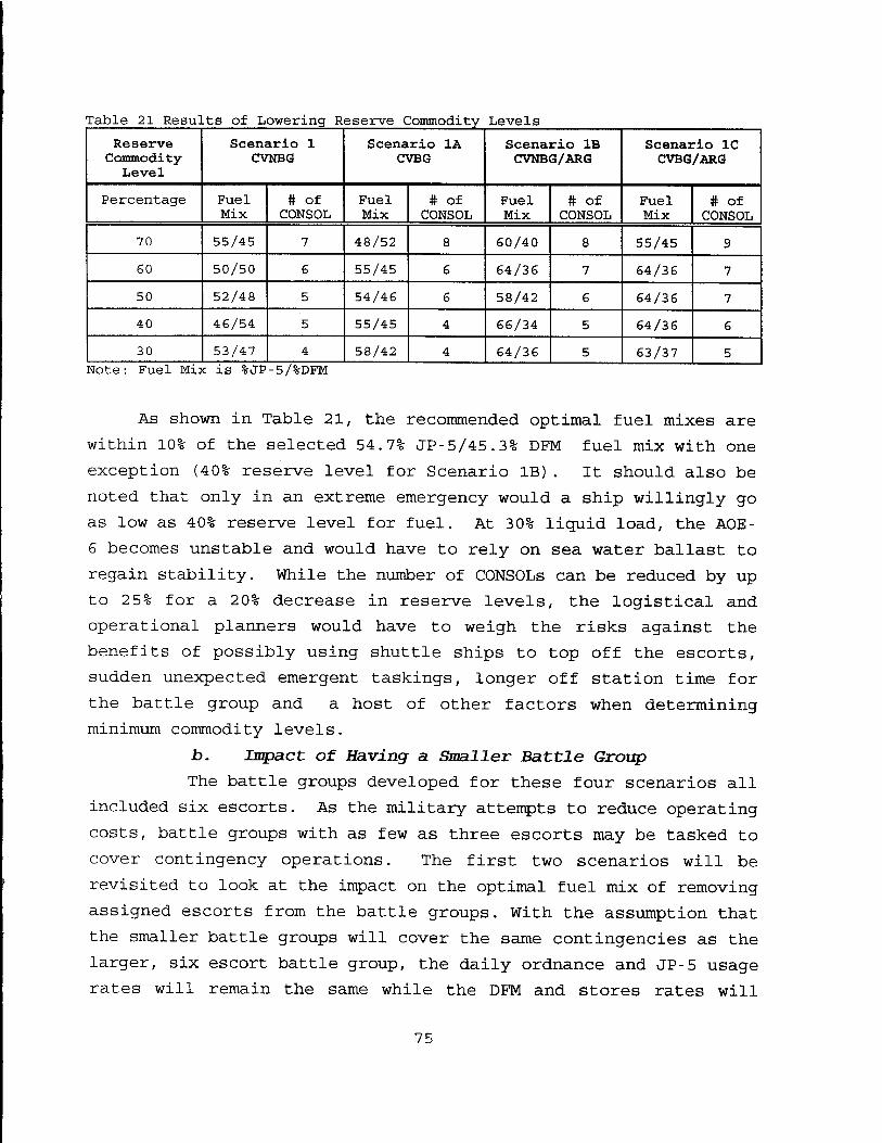
Table 21 Results of Lowering Reserve Commodity- Levels
Reserve Commodity
Level
Scenario 1 CVNBG
Scenario 1A CVBG
Scenario IB CVNBG/ARG
Scenario 1C CVBG/ARG
Percentage Fuel Mix
# of CONSOL
Fuel Mix
# of CONSOL
Fuel Mix
# Of CONSOL
Fuel Mix
# Of CONSOL
70 55/45 7 48/52 8 60/40 8 55/45 9
60 50/50 6 55/45 6 64/36 7 64/36 7
50 52/48 5 54/46 6 58/42 6 64/36 7
40 46/54 5 55/45 4 66/34 5 64/36 6
30 53/47 4 58/42 4 64/36 5 63/37 5 Note: Fuel Mis c is %JP -5/%DFM
As shown in Table 21, the recommended optimal fuel mixes are
within 10% of the selected 54.7% JP-5/45.3% DFM fuel mix with one
exception (40% reserve level for Scenario IB). It should also be
noted that only in an extreme emergency would a ship willingly go
as low as 40% reserve level for fuel. At 30% liquid load, the AOE-
6 becomes unstable and would have to rely on sea water ballast to
regain stability. While the number of CONSOLS can be reduced by up
to 25% for a 20% decrease in reserve levels, the logistical and
operational planners would have to weigh the risks against the
benefits of possibly using shuttle ships to top off the escorts,
sudden unexpected emergent taskings, longer off station time for
the battle group and a host of other factors when determining
minimum commodity levels.
b. Impact of Having a Smaller Battle Group
The battle groups developed for these four scenarios all
included six escorts. As the military attempts to reduce operating
costs, battle groups with as few as three escorts may be tasked to
cover contingency operations. The first two scenarios will be
revisited to look at the impact on the optimal fuel mix of removing
assigned escorts from the battle groups. With the assumption that
the smaller battle groups will cover the same contingencies as the
larger, six escort battle group, the daily ordnance and JP-5 usage
rates will remain the same while the DFM and stores rates will
75
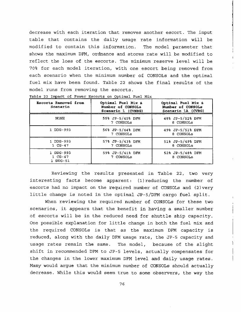
decrease with each iteration that removes another escort. The input
table that contains the daily usage rate information will be
modified to contain this information. The model parameter that
shows the maximum DFM, ordnance and stores rate will be modified to
reflect the loss of the escorts. The minimum reserve level will be
70% for each model iteration, with one escort being removed from
each scenario when the minimum number of CONSOLS and the optimal
fuel mix have been found. Table 22 shows the final results of the
model runs from removing the escorts.
Table 22 Impact of Fewer Escorts on Optimal Fuel Mix
Escorts Removed from Scenario
Optimal Fuel Mix & Number of CONSOLS Scenario 1 (CVNBG)
Optimal Fuel Mix & Number of CONSOLS Scenario 1A (CVBG)
NONE 55% JP-5/45% DFM 7 CONSOLS
48% JP-5/52% DFM 8 CONSOLS
1 DDG-993 56% JP-5/44% DFM 7 CONSOLS
49% JP-5/51% DFM 8 CONSOLS
1 DDG-993 1 CG-47
57% JP-5/43% DFM 7 CONSOLS
51% JP-5/49% DFM 8 CONSOLS
1 DDG-993 1 CG-47 1 DDG-51
59% JP-5/41% DFM 7 CONSOLS
52% JP-5/48% DFM 8 CONSOLS
Reviewing the results presented in Table 22, two very
interesting facts become apparent: (1)reducing the number of
escorts had no impact on the required number of CONSOLS and (2)very
little change is noted in the optimal JP-5/DFM cargo fuel split.
When reviewing the required number of CONSOLS for these two
scenarios, it appears that the benefit in having a smaller number
of escorts will be in the reduced need for shuttle ship capacity.
One possible explanation for little change in both the fuel mix and
the required CONSOLS is that as the maximum DFM capacity is
reduced, along with the daily DFM usage rate, the JP-5 capacity and
usage rates remain the same. The model, because of the slight
shift in recommended DFM to JP-5 levels, actually compensates for
the changes in the lower maximum DFM level and daily usage rates.
Many would argue that the minimum number of CONSOLS should actually
decrease. While this would seem true to some observers, the way the
76
program is modelled prevents this fact from coming to light. One
key element is that the operation ceases at day 80, causing an "end
effect". This means that the ships in the battle group can be
replenished with CONSOL 7 at day 72 and be at 71% on day 80, or the
battle group can be replenished on day 79 and be at 98% on day 80.
The objective function prefers the second alternative, but the
model must first find a feasible solution. In real life, another
CONSOL would be scheduled for day 82 as the ships departed station
for the first battle group. It is a very real possibility that the
scenario is not long enough to produce an appreciable difference in
the required number of CONSOLS. In the case of the scenarios
involving the conventional powered carrier, the primary reason for
for no meaningful difference in the number of CONSOLS is that the
escorts have and use such a small percentage of DFM (and stores)
relative to the CV.
The most important information gained from these results, is
that even with changing CVBG compositions, the recommended fuel
mixes all are within 7% of the selected 44.7% JP-5/54.3% DFM cargo
fuel split.
E. SUBSTITUTING THE AOE-1 CLASS FOR THE AOE-6 CLASS AS THE
ASSIGNED BATTLE GROUP STATION SHIP
As the Navy moves into the 21st century, it is readily
apparent that only eight station ships, four in the AOE-1 class and
four in the AOE-6 class, will be available to deploy with the
currently projected 12 carrier battle groups. This thesis
investigates the design features of the AOE-6 class in depth, as
well as analyzing the commodity storage capacities and how those
capacities impact CVBG operations. While it is readily apparent
that the habitability, combat survivability and the overall
shipboard living environment will be much better on a newly
constructed AOE-6 class ship as opposed to the aging AOE-1 class
ship, will the cost saving design decisions that removed 56 feet of
ship length from the AOE-6 class materialize into a problem that
will possibly impact fleet operation well into the next century?
77
In an attempt to examine this question, both GAMS programs were
edited to contain data for an AOE-1 class station ship, instead of
the AOE-6.
The motivation for examining this particular problem originated
at Naval Weapons Station, Earle, NJ. The lead load planner, Mr.
Robert Aten, conducted a shipboard survey of the ammunition holds
aboard the USS Supply, located in Norfolk, VA. After taking
measurements of the ordnance holds, it became apparent that the
AOE-6 did indeed have much less storage volume then the AOE-1
class. When this information became available to CINCLANTFLT, Mr.
Aten was directed via the chain of command to take the USS Seattle
(AOE 3) tailored load list [Ref. 23] and load that aboard the AOE-6
[Ref. 15]. As Mr. Aten had anticipated, the Seattle's tailored load
list was not able to be loaded aboard Supply, forcing Mr. Aten to
ask his superiors for guidance on which ordnance types to drop from
the list. The second motivation was provided by Mr. Marvin Miller
of the Underway Replenishment Department, Port Hueneme Division of
the Naval Surface Warfare Center. During a phone interview with
Mr. Miller, he expressed concern over the loss of one UNREP station
and the deletion of the fourth ammunition hold [Ref. 19] . His
primary concern was that the Navy had spent a great deal of time,
money and effort to bring the AOE-6 class into the fleet and that
the Navy may have actually purchased less commodity capacity than
a class of ships already in the fleet. When Mr. Miller was
informed of the topic and scope of this thesis, he stated that it
might be useful to run the same battle group commodity program and
see just how much of a difference exists between the AOE-1 and the
AOE-6 classes.
1. Ordnance Load Model
To convert the optimal load list program from loading an AOE
6 class ship to loading an AOE 1 class (parameters for USS Seattle
(AOE 3) were used for this thesis) the following parameters in the
model were modified from those shown in Appendix I:
Indices - the number of storage decks aboard ship increased from 11 to 20.
78
Input Data - CUBED and STRESSD were changed to match the volume and deck stress of AOE 3 [Refs. 16 and 21] .
Equations - The equations representing the stability- constraints were edited to be applicable to the AOE 3.
The first model runs with this data provided some interesting
results. What the model would do to circumvent the stability-
constraint, was to load a very large number of weapon accessories
into the necessary holds. While these accessories added no value
to the objective function, they did increase the total tonnage of
the ordnance loadout with relatively useless items such as 1500
MK46 igniter kits. A second modification was made to the required
accessory constraint to ensure that the model only loaded the same
number of accessories as weapons. This was not necessary for the
AOE-6 model run as volume was the only constraint for that model.
These changes and the results of the model run for these changes
are available in Appendix J.
The first, direct method of comparison is the overall
objective function value. For the AOE 3 model run, the objective
function value was 128,693.3473 as compared to 109,972.8734 for the
AOE 6 model. Again, with only two model runs, it is very hard to
determine any magnitude to the difference of the two objective
functions. The only conclusion supportable from this information
is that the AOE-3 ordnance load is some magnitude better then the
AOE-6 ordnance load. The second method of comparison is total
tonnage. The total ordnance tonnage for the AOE-3 model is
2,905.28 tons as compared to the AOE-6 tonnage of 2,354.31. Table
2 3 shows a direct comparison of the number of each weapon loaded
aboard AOE-3 and AOE-6.
79
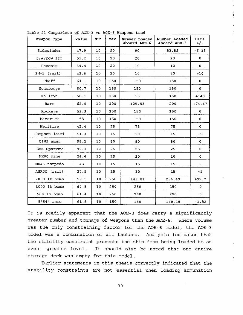
Table 23 Comparison of AOE- 3 vs AOE-6 Weapons Load
Weapon Type Value Min Max Number Loaded Aboard AOE-6
Number Loaded Aboard AOE-3
Diff */-
Sidewinder 47.9 10 90 90 83.85 -6.15
Sparrow III 51.2 10 20 20 20 0
Phoenix 34.4 10 20 10 10 0
SM-2 (rail) 43.6 10 20 10 20 +10
Chaff 64.1 10 150 150 150 0
Sonobouys 60.7 10 150 150 150 0
Walleye 58.1 10 150 10 150 +140
Harm 62.9 10 200 125.53 200 +74.47
Rockeye 53.3 10 150 150 150 0
Maverick 58 10 150 150 150 0
Hellfire 42.4 10 75 75 75 0
Harpoon (air) 44.3 10 15 10 15 +5
CIWS ammo 58.1 10 80 80 80 0
Sea Sparrow 49.1 10 25 25 25 0
MK60 mine 24.6 10 25 10 10 0
MK46 torpedo 43 10 15 15 15 0
ASROC (rail) 27.5 10 15 10 15 +5
2000 lb bomb 59.5 10 250 143.81 236.49 +92.7
1000 lb bomb 64.5 10 250 250 250 0
500 lb bomb 61.4 10 250 250 250 0
5'54" ammo 61.8 10 150 150 148.18 -1.82
It is readily apparent that the AOE-3 does carry a significantly
greater number and tonnage of weapons then the AOE-6. Where volume
was the only constraining factor for the AOE-6 model, the AOE-3
model was a combination of all factors. Analysis indicates that
the stability constraint prevents the ship from being loaded to an
even greater level. It should also be noted that one entire
storage deck was empty for this model.
Earlier statements in this thesis correctly indicated that the
stability constraints are not essential when loading ammunition
80
aboard an AOE. When loading 3,000 tons of ordnance aboard an AE,
it is vitally important for ship's stability that the weight be
distributed properly. The addition of 3,000 tons of ordnance on an
AOE does not impose the same constraints. With an AOE, the weight
of seven million gallons of cargo fuel, stored forward and low in
the ship, as well as over one million gallons of bunker fuel, can
compensate for the placement of the ordnance in maintainig the
ship's stability. Another model run was completed for both the
AOE-6 and the AOE-3 models with the stability constraints removed.
As expected, there was no change for the AOE-6, as that model run
was constrained by the available storage volume of the ship. The
AOE-3 class showed a drastic change. Table 24 shows a comparison
of the AOE-6, the AOE-3 with stability constraints and then the
AOE-3 without stability constraints.
81
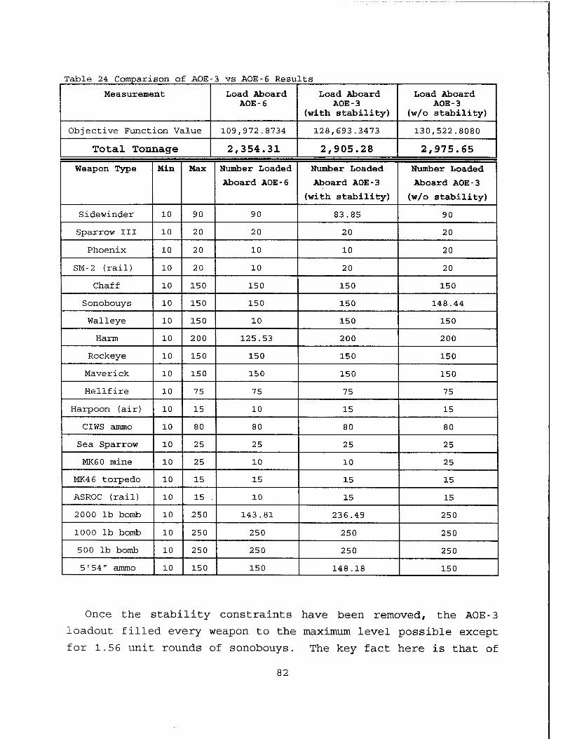
Table 24 Comparison of AOE- 3 vs AOE-6 Results
Measurement Load Aboard AOE-6
Load Aboard AOE-3
(with stability)
Load Aboard AOE-3
(w/o stability)
Objective Function Value 109,972.8734 128,693.3473 130,522.8080
Total Tonnage 2,354.31 2,905.28 2,975.65
Weapon Type Min Max Number Loaded
Aboard AOE-6
Number Loaded
Aboard AOE-3
(with stability)
Number Loaded
Aboard AOE-3
(w/o stability)
Sidewinder 10 90 90 83.85 90
Sparrow III 10 20 20 20 20
Phoenix 10 20 10 10 20
SM-2 (rail) 10 20 10 20 20
Chaff 10 150 150 150 150
Sonobouys 10 150 150 150 148.44
Walleye 10 150 10 150 150
Harm 10 200 125.53 200 200
Rockeye 10 150 150 150 150
Maverick 10 150 150 150 150
Hellfire 10 75 75 75 75
Harpoon (air) 10 15 10 15 15
CIWS ammo 10 80 80 80 80
Sea Sparrow 10 25 25 25 25
MK60 mine 10 25 10 10 25
MK4 6 torpedo 10 15 15 15 15
ASROC (rail) 10 15 10 15 15
2000 lb bomb 10 250 143.81 236.49 250
1000 lb bomb 10 250 250 250 250
500 lb bomb 10 250 250 250 250
5'54" ammo 10 150 150 148.18 150
Once the stability constraints have been removed, the AOE-3
loadout filled every weapon to the maximum level possible except
for 1.56 unit rounds of sonobouys. The key fact here is that of
82
the 2 0 storage decks, nine were volume constrained, four were
weight constrained and one deck was compatibility constrained. One
deck was completely empty! It is clear that with some structural
reinforcement to the decks that are weight constrained, 11 storage
decks for the AOE-3 class still have room to load more ordnance
aboard the ship. Even with the stability constraints, a larger,
more diverse load list will still permit the AOE-3 to carry up to
3 0% more of an ordnance loadout then the AOE-6.
2. Cargo Fuel Model
When comparing the performance of the AOE-6 class to the AOE-1
class, the only area that can be measured is the difference in the
required number of CONSOLS for the two station ships. During the
comparison of the AOE-6 and the AOE-3 in the previous section, it
is readily apparent that the Seattle (AOE 3) can carry more
ordnance then the Supply (AOE 6). Ordnance however, was never a
limiting factor in any scenario. The AOE-1 class also carries more
dry and refrigerated stores then the AOE-6. However, fuel, DFM and
JP-5, was the limiting factor. The question that needs to be
answered is: Does the convertible tank design of the AOE-6 class
give that ship enough flexibility to compensate for more storage
capacity aboard the AOE-1 class?
To convert the GAMS model from the AOE-6 to the AOE-1 station
ship, the variable INITAOE was deleted, and the parameter MAXLEVEL
was changed to match the battle group commodity totals with the
AOE-1 as the station ship. Table 25 shows the comparison in the
minimum required number of CONSOLS for each Scenario with an AOE-6
and then with an AOE-1 class station ship. The AOE-6 and AOE-1 have
the same unclassified ship's ordnance loadout, the same ship's
cargo loadout, and the same ship's bunker fuel loadout. As for
cargo fuel, the AOE-1 has roughly a 7.2 million gallon capacity
(stow factor included), with a fixed 40% JP-5, or 2,669,177 gallons
JP-5, and 60% DFM, or 4,460,344 gallons DFM. The AOE-1 contains an
extra 15 thousand cubic feet, or 113.4 tons of stores capacity
over the AOE-6 as well as a 30 thousand cubic feet, or a design
load of 400 tons, of extra capacity for weapons over the AOE-6. The
83
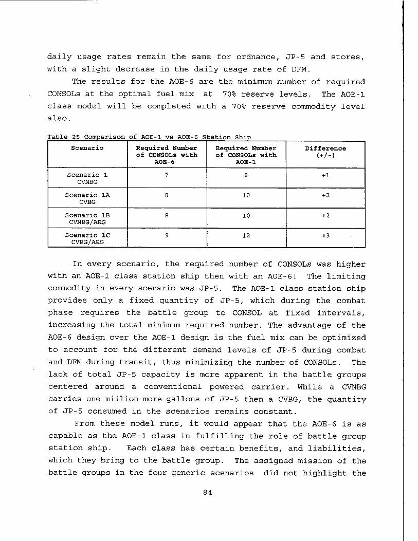
daily usage rates remain the same for ordnance, JP-5 and stores,
with a slight decrease in the daily usage rate of DFM.
The results for the AOE-6 are the minimum number of required
CONSOLS at the optimal fuel mix at 70% reserve levels. The AOE-1
class model will be completed with a 70% reserve commodity level
also.
Table 25 Comparison of AOE-1 vs AOE-6 Station Ship
Scenario Required Number of CONSOLS with
AOE-6
Required Number of CONSOLS with
AOE-1
Difference (+/-)
Scenario 1 CVNBG
7 8 +1
Scenario 1A CVBG
8 10 +2
Scenario IB CVNBG/ARG
8 10 +2
Scenario 1C CVBG/ARG
9 12 +3
In every scenario, the required number of CONSOLS was higher
with an AOE-1 class station ship then with an AOE-6! The limiting
commodity in every scenario was JP-5. The AOE-1 class station ship
provides only a fixed quantity of JP-5, which during the combat
phase requires the battle group to CONSOL at fixed intervals,
increasing the total minimum required number. The advantage of the
AOE-6 design over the AOE-1 design is the fuel mix can be optimized
to account for the different demand levels of JP-5 during combat
and DFM during transit, thus minimizing the number of CONSOLS. The
lack of total JP-5 capacity is more apparent in the battle groups
centered around a conventional powered carrier. While a CVNBG
carries one miilion more gallons of JP-5 then a CVBG, the quantity
of JP-5 consumed in the scenarios remains constant.
From these model runs, it would appear that the AOE-6 is as
capable as the AOE-1 class in fulfilling the role of battle group
station ship. Each class has certain benefits, and liabilities,
which they bring to the battle group. The assigned mission of the
battle groups in the four generic scenarios did not highlight the
84
higher weapons or stores storage capacities of the AOE-1 class, but
instead highlighted the flexibility that the convertible tanks
bring to the AOE-6 class. The results for this model are based on
the AOE-1 class ships having a cargo fuel mix that contains 40%
JP-5/60% DFM. With proper tank alignment, the AOE-1 class can also
be configured to carry a 55% JP-5/45% DFM cargo fuel mix. Future
plans call for the entire AOE-1 class to undergo an extensive
Service Life Extension Program (SLEP) at the end of this century.
This SLEP period would provide an excellent opportunity to
reconfigure all four ships in the AOE-1 class to support a 55% JP-
5/45% DFM cargo fuel mix.
F. CONCLUSIONS
The goal of this thesis was to find the optimal loadout of the
Supply class AOE. The goal was sub-divided into two sections; the
ordnance loadout and the fuel loadout. For the ordnance loadout,
a successful computer model was developed that loaded an AOE-6 in
the same fashion as a professional load planner. This computer
model, for the first time, actually accounted for and prevented,
the loading of incompatible ordnance types in the same cargo holds.
This model has the capability, with some enhancements, to be a
valuable asset to loading all ordnance carrying ships, not just
AOEs. The model highlights the strengths and weaknesses of both
the AOE-6 and the AOE-1 class ships.
The second section, to find an optimal fuel mix, demonstrated
the inherent flexibility that convertible tanks bring to the AOE-6
class. While every scenario has a different optimal fuel mix, by
configuring the AOE-6 to carry roughly 55% JP-5/45% DFM, no change
was found in the minimum number of CONSOLS.
The Supply class AOE is an impressive ship design. Many of
the shortcomings of the AOE-1 class have been corrected and
improved. As the Navy looks to the future, it is easy to see that
the AOEs of the Sacramento (AOE 1) and Supply (AOE 6) classes will
be the mainstay of the CLF. As such, every effort must be made to
improve and upgrade both classes of ship. For the AOE 1 class,
85
this means planning, funding, and executing an ambitious SLEP that
will bring this 1950's design, 1960's built class into the 21st
century. Areas of improvement include preparing the class for the
increase in vertical launch weapons, upgrading the combat
survivability, ship's habitability, the ship's weapon systems and
UNREP gear.
For the AOE-6, this means ensuring the monorail hoist that is
currently planned actually reaches operational status. This class
of ship is impressive now, arguably the most capable replenishment
ship in the world. Allowing this class to regain the lost 56 feet
of length and it will be the premier UNREP ship well into the next
century. Think of the force multiplier you would have traveling
with each battle group with the world's most capable CLF ship.
G. RECOMMENDATIONS FOR FUTURE STUDY
1. Ordnance Load Model
While this program does an excellent job of loading a few
select weapons aboard a single class of ship, several shortcomings
will have to be corrected prior to it being of great benefit to the
fleet:
1. The program as written is extremely user unfriendly. Only
a person with adequate knowledge of GAMS would be able to operate
the program should changes in any of the parameters be needed. The
recommendation is for the development of a program, using software
such as VISUAL BASIC, that would allow for a menu driven version of
the load list program. Enhance the program by expanding the program
parameters to include the data necessary to load every ordnance
carrying ship, including CLF, aircraft carriers and amphibious ship
with every type of ordnance, by its Naval Ammunition Logistics Code
(NALC), currently in the inventory. This would allow the user to
load any ship, with any desired weapon combination. Most of this
information is unclassified and readily available at any Naval
Weapon Station.
The goal here would be to have a menu driven program that
would first give the user the option of selecting which ship class
to load. Then the user would be able to input a weapon type (by
86
NALC) , the minimum and maximum number of each weapon type, and the
associated priority rating in comparison to the other weapons
selected for the loadout. From this information, an initial load
list can be generated for review.
2. While the load list program will tell the user on which
deck to place each weapon, a method should be developed to tell the
user more specifically where on each deck to place the weapon.
This would require the program to be expanded to include many of
the stowage and dunnage factors involved with ordnance loading
aboard ship.
2 . Cargo Fuel Model
The Underway Replenishment Department of the Naval Surface
Warfare Center, Port Hueneme Division, has been looking at several
different options for reducing the total cost of UNREP, without
lowering fleet effectiveness [Ref. 4] . With the decommissioning of
the AORs and the transfer to MSC of the AE-26 class and the AFS
fleet, two options from this study remain viable and worthy of
further analysis.
The first option is to "jumboize" the AOE-6 class, similar to
the process that the AO-J 177 class recently completed. If the
AOE-6 class completed this process, her cargo fuel capacity would
increase to 190,000 barrels, or an additional 34,000 barrels. Her
cargo stores would increase by 30,000 cubic feet to 120,000 cubic
feet, and her cargo ammunition capacity would increase to 367,000
cubic feet [Ref. 4: p. 6]. With a total increase in commodity
capacity, the shuttle ship requirement would be reduced. A cost
benefit analysis of "jumboizing" the AOE-6 class as compared to the
reduced shuttle ship requirement would provide an excellent
research opportunity. The AOE-J-6 class could also be substituted
into the two models presented in this thesis to demonstrate its
expanded capability and usefulness to the fleet.
The second option involves the AOE-1 class. As mentioned in
Chapter I, this class of ship has been in service over a quarter of
a century. If the Navy intends to keep these ships as assets, a
plan must be developed to overhaul and upgrade the entire class.
87
Currently, 200,000 cubic feet of obsolete main deck handling space
is not being fully utilized. The AOE-1 was constructed at a time
when vertical launch weapons were not in the inventory. An
analysis of a plan to upgrade the stores and ammunition storage
area could demonstrate the benefit and cost effectiveness of having
the entire AOE-1 class placed through a SLEP similar to those
undertaken for the fossil fuel aircraft carriers.
The alternative to both of these recommendations is to look at
the cargo capacity requirements for the AOE of the future. Based
upon the currently planned CLF force for the year 2010, research
can be conducted into what size the station ship of the future will
have to be in relation to the future size of the CV/CVN BG and the
number of shuttle ships available. With no money currently
allocated for a follow-on class to the AOE-6, this type of research
could possibly influence the design and cost of future ship
construction.
88
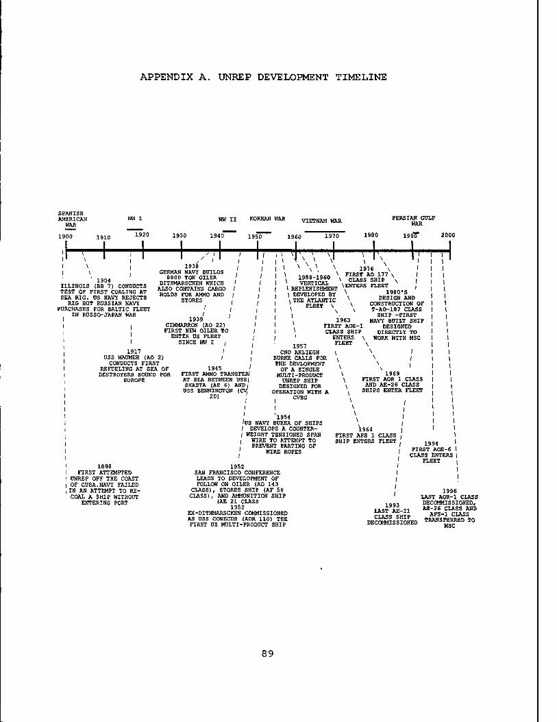
APPENDIX A. UNREP DEVELOPMENT TIMELINE
SPANISH AMERICAN WAR
KOREAN WAR VIETNAM WAR
1910 1920 1930 1940 1950 1960 1970 1980
PERSIAN GULF WAR
199T
r?—I 2000
\ I 1904
ILLINOIS (BB 7) CONDUCTS TEST OP FIRST COALING AT SEA RIG. DS NAVY REJECTS
RIG BDT RUSSIAN NAVY PURCHASES FOR BALTIC FLEET
IN RUSSO-JAPAN WAR
I
/ I 1938
GERMAN NAVY BUILDS 8800 TON OILER
DITHMARSCKEN WHICH ALSO CONTAINS CARGO HOLDS FOR AMMO AND
STORES
/ 1939
CIMMARRON (AO 22) FIRST NEW OILER TO ENTER US FLEET
SINCE WW I
\ \ \
, 1958-1960 1 VERTICAL \ REPLENISHMENT \ DEVELOPED BY i THE ATLANTIC , FLEET \
\ \
1976 \ FIRST AO 177 \
\ CLASS SHIP \ \ENTERS FLEET \
\ \ 1963
FIRST AOE-1 CLASS SHIP
/ 1917
USS MAUMEE (AO 2) CONDUCTS FIRST
REFUELING AT SEA OF DESTROYERS BOUND FOR
EUROPE
' I
1945 ' FIRST AMMO TRANSFER/ AT SEA BETWEEN USS| SHASTA (AE 6) ANDi DSS BENNINGTON (CV
20) *
1957 CNO ARLIEGH
BURKE CALLS FOR THE DEVLOPMENT OF A SINGLE
MULTI-PRODUCT UNREP SHIP DESIGNED FOR
OPERATION WITH A CVBG
ENTERS FLEET
1980'S DESIGN AND
CONSTRUCTION OF T-AO-187 CLASS SHIP -FIRST
NAVY BUILT SHIP DESIGNED
DIRECTLY TO WORK WITH MSC
\ /
1969 FIRST AOR 1 CLASS AND AE-26 CLASS SHIPS ENTER FLEET
1954 'US NAVY BUREA OF SHIPS 1 DEVELOPS A COUNTER- / WEIGHT TENSIONED SPAN i WIRE TO ATTEMPT TO
, PREVENT PARTING OF ' WIRE ROPES
\ \ 1964
FIRST AFS 1 CLASS SHIP ENTERS FLEET
1898 FIRST ATTEMPTED
UNREP OFF THE COAST OF CUBA.NAVY FAILED IN AN ATTEMPT TO RE- COAL A SHIP WITHOUT
ENTERING PORT
1952 SAN FRANCISCO CONFERENCE LEADS TO DEVELOPMENT OF FOLLOW ON OILER (AO 143
CLASS), STORES SHIP (AF 58 CLASS), AND AMMUNITION SHIP
(AE 21 CLASS 1952
EX-DITHMARSCKEN COMMISSIONED AS USS CONECUH (AOR 110) THE FIRST US MULTI-PRODUCT SHIP
1994 FIRST AOE- CLASS ENTERS
FLEET
1993 LAST AE-21 CLASS SHIP
DECOMMISSIONED
1996 LAST AOR-1 CLASS DECOMMISSIONED, AE-26 CLASS AND
AFS-1 CLASS TRANSFERRED TO
MSC
89
90
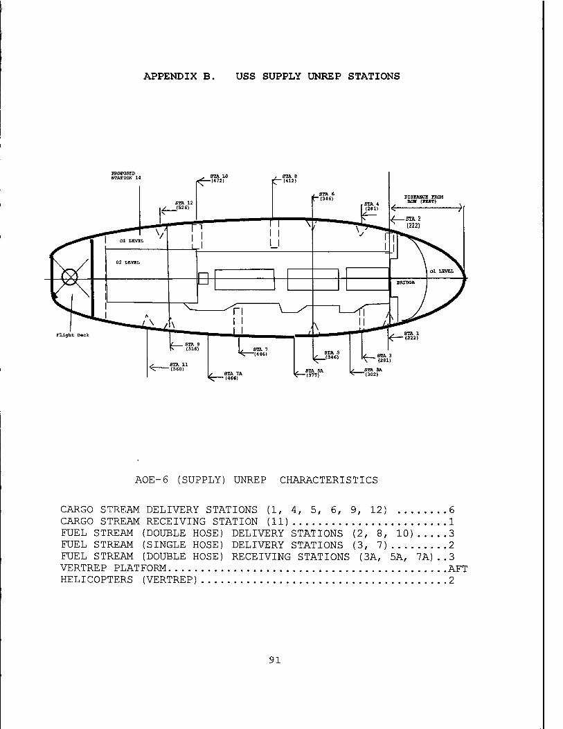
APPENDIX B. USS SUPPLY UNREP STATIONS
PROPOSED STATION 14 . STA 10
r\~~(472) STA e "(412)
, STA 6 l (346) DISTANCE FROH
BOV (FEET)
Flight Deck
. STA 9 (516)
/ STA 11 X (560)
STA 7 -(446)
kr- STA 7A (466)
K~< STA 5 ,(34«)
ly. STA 5A 'S—(377)
, STA 1 ^ (222)
STA 3 ' (261)
STA 3A "(302)
AOE-6 (SUPPLY) UNREP CHARACTERISTICS
CARGO STREAM DELIVERY STATIONS (1, 4, 5, 6, 9, 12) 6 CARGO STREAM RECEIVING STATION (11) 1 FUEL STREAM (DOUBLE HOSE) DELIVERY STATIONS (2, 8, 10) 3 FUEL STREAM (SINGLE HOSE) DELIVERY STATIONS (3, 7) 2 FUEL STREAM (DOUBLE HOSE) RECEIVING STATIONS (3A, 5A, 7A)..3 VERTREP PLATFORM AFT HELICOPTERS (VERTREP) 2
91

92
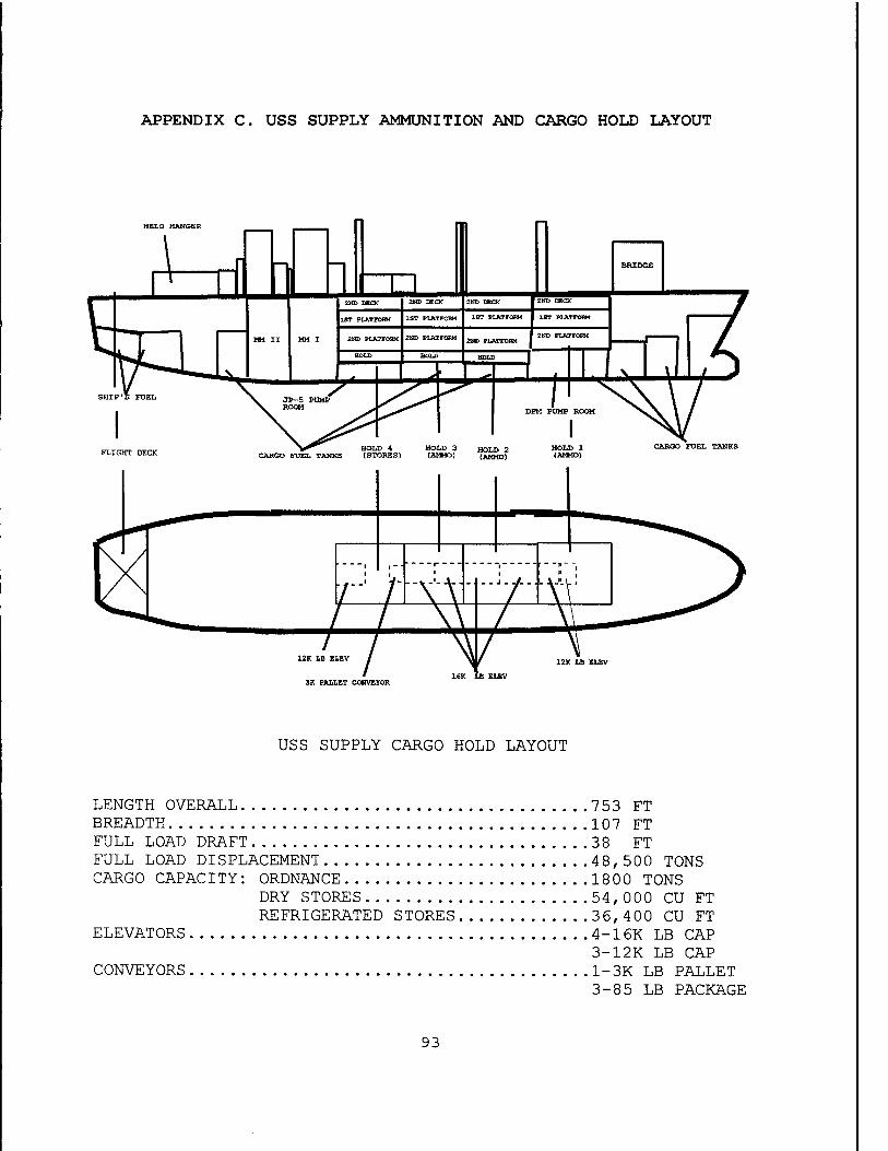
APPENDIX C. USS SUPPLY AMMUNITION AND CARGO HOLD LAYOUT
HELO HANGER
12K LB ELEV
3K PALLET CONVEYOR
12K LB ELEV
16K LB ELEV
USS SUPPLY CARGO HOLD LAYOUT
LENGTH OVERALL 753 FT BREADTH 107 FT FULL LOAD DRAFT 38 FT FULL LOAD DISPLACEMENT 48,500 TONS CARGO CAPACITY: ORDNANCE 1800 TONS
DRY STORES 54,000 CU FT REFRIGERATED STORES 36,400 CU FT
ELEVATORS 4-16K LB CAP 3-12K LB CAP
CONVEYORS 1-3K LB PALLET 3-85 LB PACKAGE
93
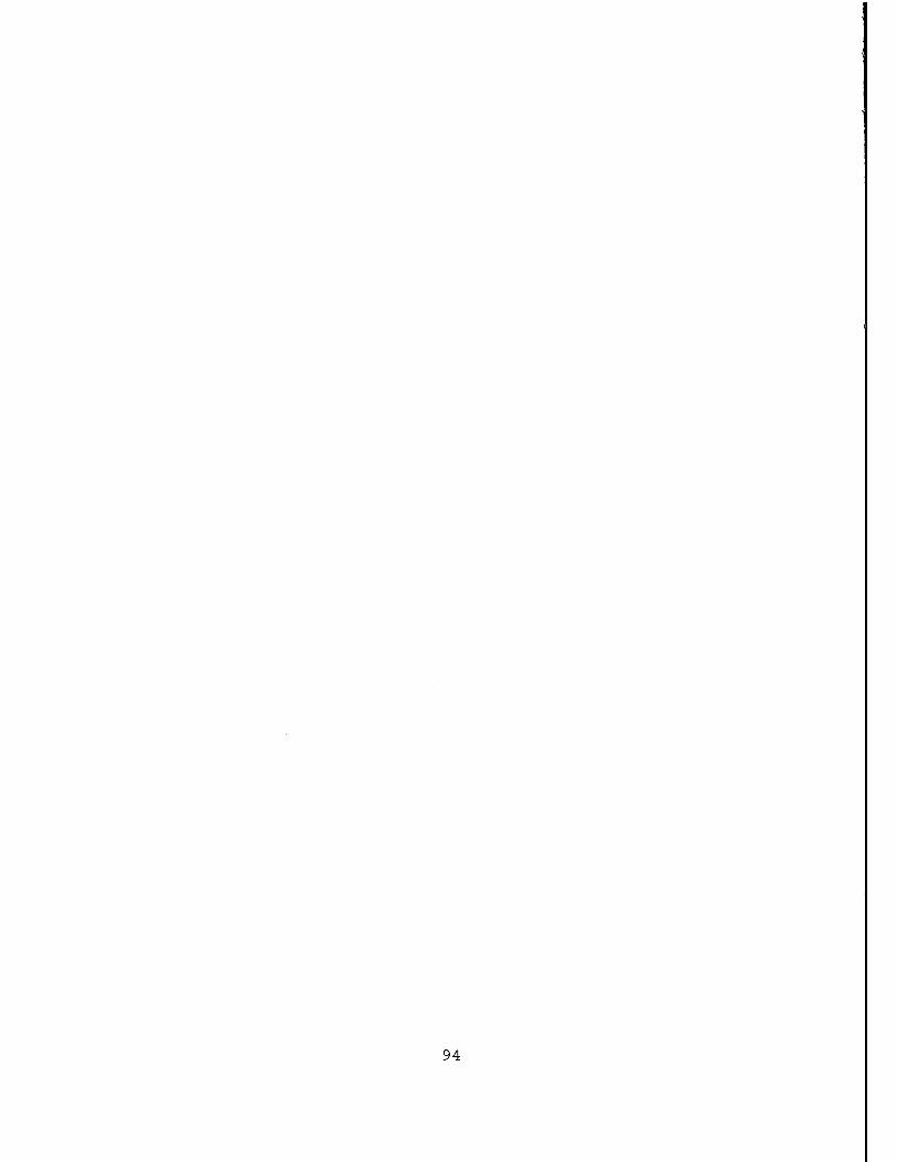
94
APPENDIX D. USS SUPPLY CARGO FUEL TANK AND PUMP ROOM LAYOUT
* "9
ta u>to M-4 CD 1
1 cr»o
WH» ta
P> •% MS ta Ci
95

96
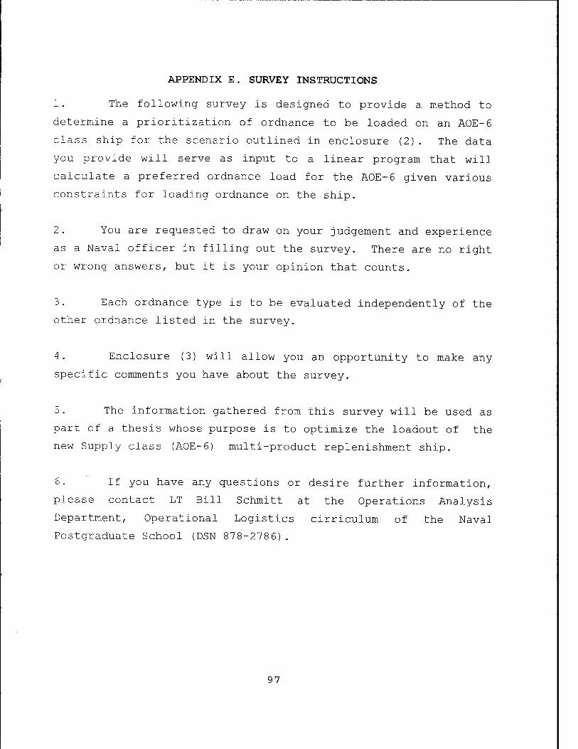
APPENDIX E. SURVEY INSTRUCTIONS
1. The following survey is designed to provide a method to
determine a prioritization of ordnance to be loaded on an AOE-6
class ship for the scenario outlined in enclosure (2). The data
you provide will serve as input to a linear program that will
calculate a preferred ordnance load for the AOE-6 given various
constraints for loading ordnance on the ship.
2. You are requested to draw on your judgement and experience
as a Naval officer in filling out the survey. There are no right
or wrong answers, but it is your opinion that counts.
3. Each ordnance type is to be evaluated independently of the
other ordnance listed in the survey.
4. Enclosure (3) will allow you an opportunity to make any
specific comments you have about the survey.
5. The information gathered from this survey will be used as
part of a thesis whose purpose is to optimize the loadout of the
new Supply class (AOE-6) multi-product replenishment ship.
6. If you have any questions or desire further information,
please contact LT Bill Schmitt at the Operations Analysis
Department, Operational Logistics cirriculum of the Naval
Postgraduate School (DSN 878-2786).
97
98
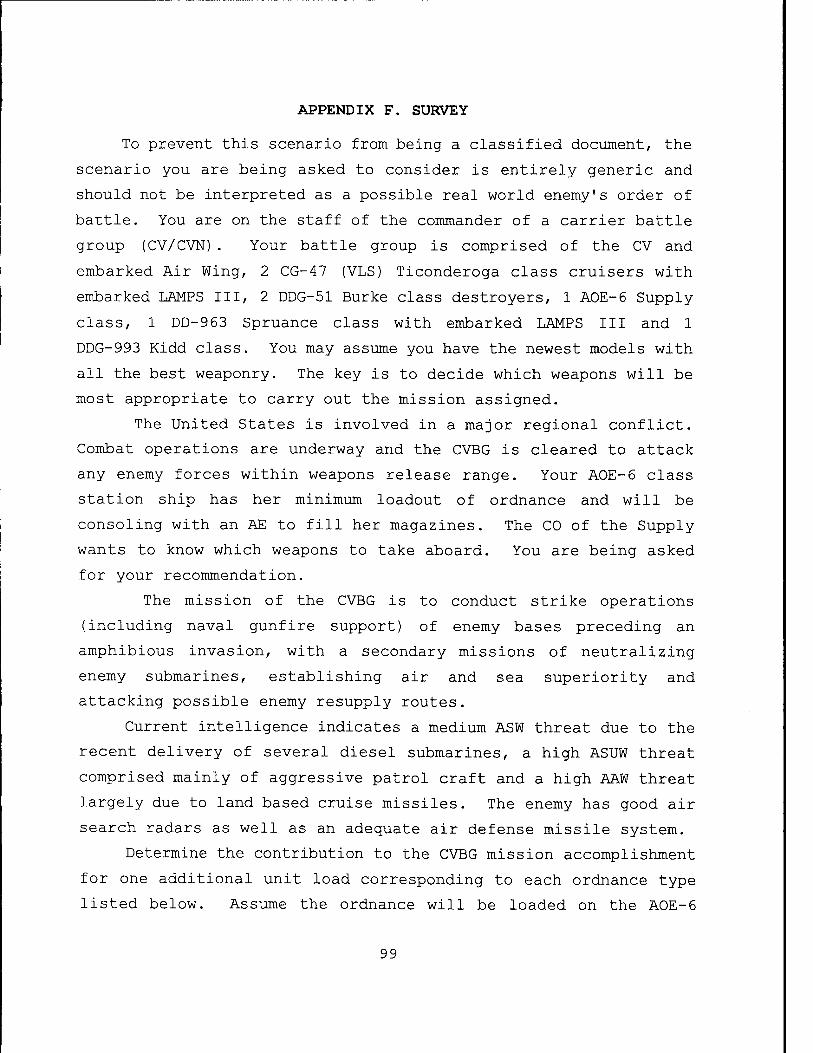
APPENDIX F. SURVEY
To prevent this scenario from being a classified document, the
scenario you are being asked to consider is entirely generic and
should not be interpreted as a possible real world enemy's order of
battle. You are on the staff of the commander of a carrier battle
group (CV/CVN) . Your battle group is comprised of the CV and
embarked Air Wing, 2 CG-47 (VLS) Ticonderoga class cruisers with
embarked LAMPS III, 2 DDG-51 Burke class destroyers, 1 AOE-6 Supply
class, 1 DD-963 Spruance class with embarked LAMPS III and 1
DDG-993 Kidd class. You may assume you have the newest models with
all the best weaponry. The key is to decide which weapons will be
most appropriate to carry out the mission assigned.
The United States is involved in a major regional conflict.
Combat operations are underway and the CVBG is cleared to attack
any enemy forces within weapons release range. Your AOE-6 class
station ship has her minimum loadout of ordnance and will be
consoling with an AE to fill her magazines. The CO of the Supply
wants to know which weapons to take aboard. You are being asked
for your recommendation.
The mission of the CVBG is to conduct strike operations
(including naval gunfire support) of enemy bases preceding an
amphibious invasion, with a secondary missions of neutralizing
enemy submarines, establishing air and sea superiority and
attacking possible enemy resupply routes.
Current intelligence indicates a medium ASW threat due to the
recent delivery of several diesel submarines, a high ASUW threat
comprised mainly of aggressive patrol craft and a high AAW threat
largely due to land based cruise missiles. The enemy has good air
search radars as well as an adequate air defense missile system.
Determine the contribution to the CVBG mission accomplishment
for one additional unit load corresponding to each ordnance type
listed below. Assume the ordnance will be loaded on the AOE-6
99
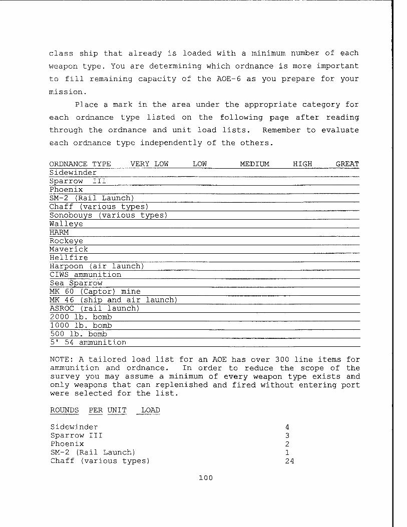
class ship that already is loaded with a minimum number of each
weapon type. You are determining which ordnance is more important
to fill remaining capacity of the AOE-6 as you prepare for your
mission.
Place a mark in the area under the appropriate category for
each ordnance type listed on the following page after reading
through the ordnance and unit load lists. Remember to evaluate
each ordnance type independently of the others.
ORDNANCE TYPE VERY LOW LOW MEDIUM HIGH GREAT Sidewinder Sparrow III Phoenix SM-2 (Rail Launch) Chaff (various types) Sonobouys (various types) Walleye HARM Rockeye Maverick Hellfire Harpoon (air launch) CIWS ammunition Sea Sparrow MK 60 (Captor) mine MK 4 6 (ship and air launch) ASROC (rail launch) 2000 lb. bomb 1000 lb. bomb 500 lb. bomb 5' 54 ammunition
NOTE: A tailored load list for an AOE has over 300 line items for ammunition and ordnance. In order to reduce the scope of the survey you may assume a minimum of every weapon type exists and only weapons that can replenished and fired without entering port were selected for the list.
ROUNDS PER UNIT LOAD
Sidewinder Sparrow III Phoenix SM-2 (Rail Launch) Chaff (various types)
4 3 2 1 24
100
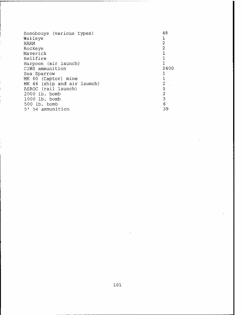
Sonobouys (various types) 48 Walleye 1 HARM 2 Rockeye 2 Maverick 1 Hellfire 1 Harpoon (air launch) 1 CIWS ammunition 2400 Sea Sparrow 1 MK 60 (Captor) mine 1 MK 4 6 (ship and air launch) 2 ASROC (rail launch) 1 2000 lb. bomb 2 1000 lb. bomb 3 500 lb. bomb 6 5' 54 ammunition 39
101
102
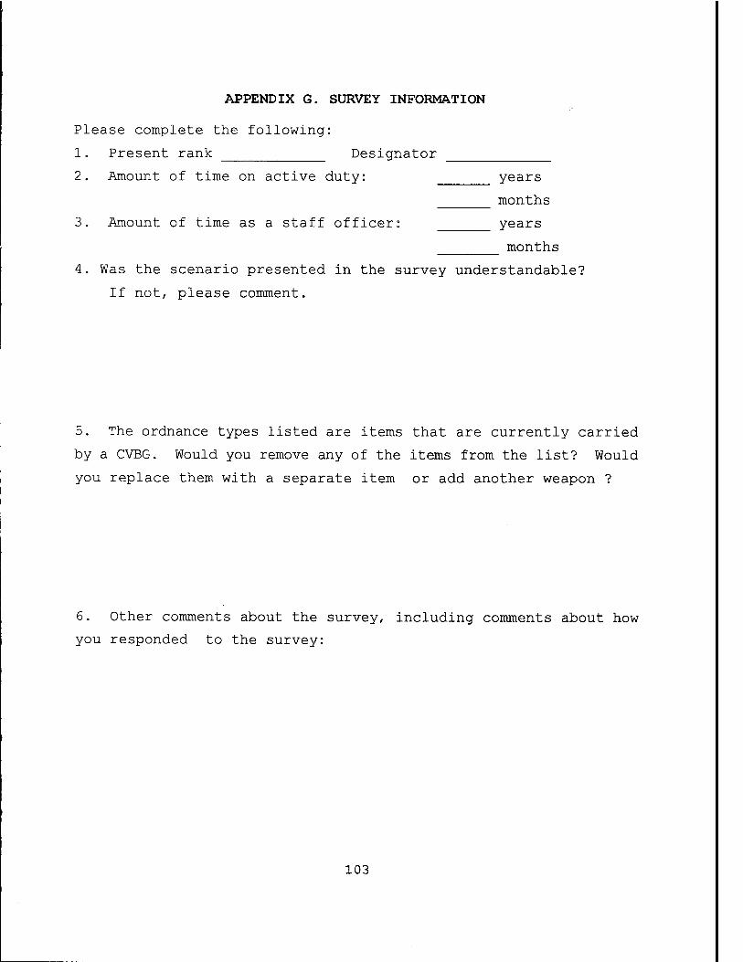
APPENDIX G. SURVEY INFORMATION
Please complete the following:
1. Present rank Designator
2. Amount of time on active duty:
3. Amount of time as a staff officer:
years
months
years
months
4. Was the scenario presented in the survey understandable?
If not, please comment.
5. The ordnance types listed are items that are currently carried
by a CVBG. Would you remove any of the items from the list? Would
you replace them with a separate item or add another weapon ?
6. Other comments about the survey, including comments about how
you responded to the survey:
103
104
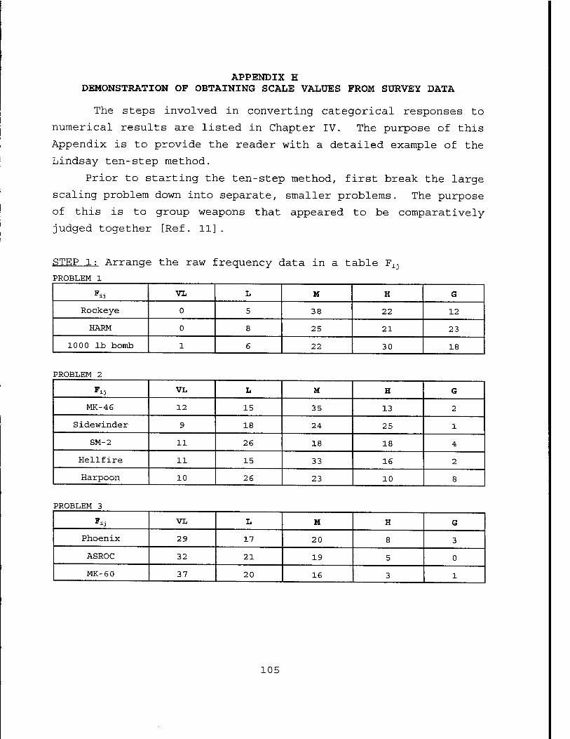
APPENDIX H DEMONSTRATION OF OBTAINING SCALE VALUES FROM SURVEY DATA
The steps involved in converting categorical responses to
numerical results are listed in Chapter IV. The purpose of this
Appendix is to provide the reader with a detailed example of the
Lindsay ten-step method.
Prior to starting the ten-step method, first break the large
scaling problem down into separate, smaller problems. The purpose
of this is to group weapons that appeared to be comparatively-
judged together [Ref. 11].
STEP 1: Arrange the raw frequency data in a table F±j PROBLEM 1
Fi: VL L M H G
Rockeye 0 5 38 22 12
HARM 0 8 25 21 23
1000 lb bomb 1 6 22 30 18
PROBLEM 2
p VL L M H G
MK-46 12 15 35 13 2
Sidewinder 9 18 24 25 1
SM-2 11 26 18 18 4
Hellfire 11 15 33 16 2
Harpoon 10 26 23 10 8
PROBLEM 3
^ VL L M H G
Phoenix 29 17 20 8 3
ASROC 32 21 19 5 0
MK-60 37 20 16 3 1
105
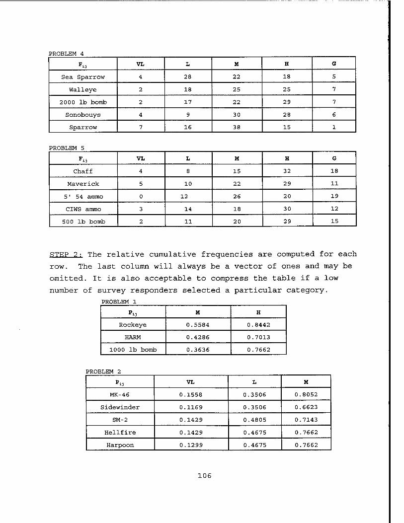
PROBLEM 4
F VL L M H G
Sea Sparrow 4 28 22 18 5
Walleye 2 18 25 25 7
2000 lb bomb 2 17 22 29 7
Sonobouys 4 9 30 28 6
Sparrow 7 16 38 15 1
PROBLEM 5
F VL L M H G
Chaff 4 8 15 32 18
Maverick 5 10 22 29 11
5' 54 ammo 0 12 26 20 19
CIWS ammo 3 14 18 30 12
500 lb bomb 2 11 20 29 15
STEP 2: The relative cumulative frequencies are computed for each
row. The last column will always be a vector of ones and may be
omitted. It is also acceptable to compress the table if a low
number of survey responders selected a particular category. PROBLEM 1
Pii M H
Rockeye 0.5584 0.8442
HARM 0.4286 0.7013
1000 lb bomb 0.3636 0.7662
PROBLEM 2
Pi3 VL L M
MK-46 0.1558 0.3506 0.8052
Sidewinder 0.1169 0.3506 0.6623
SM-2 0.1429 0.4805 0.7143
Hellfire 0.1429 0.4675 0.7662
Harpoon 0.1299 0.4675 0.7662
106
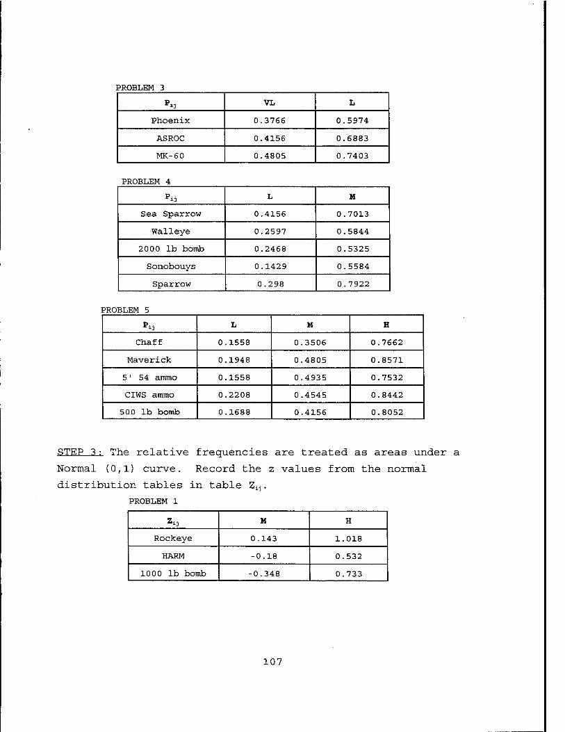
PROBLEM 3
p« VL L
Phoenix 0.3766 0.5974
ASROC 0.4156 0.6883
MK-60 0.4805 0.7403
PROBLEM 4
pii L M
Sea Sparrow 0.4156 0.7013
Walleye 0.2597 0.5844
2000 lb bomb 0.2468 0.5325
Sonobouys 0.1429 0.5584
Sparrow 0.298 0.7922
PROBLEM 5
Pi3 L M H
Chaff 0.1558 0.3506 0.7662
Maverick 0.1948 0.4805 0.8571
5' 54 ammo 0.1558 0.4935 0.7532
CIWS ammo 0.2208 0.4545 0.8442
500 lb bomb 0.1688 0.4156 0.8052
STEP 3: The relative frequencies are treated as areas under a
Normal (0,1) curve. Record the z values from the normal
distribution tables in table Zi:j.
PROBLEM 1
Zi3 M H
Rockeye 0.143 1.018
HARM -0.18 0.532
1000 lb bomb -0.348 0.733
107
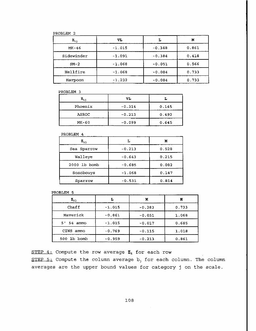
PROBLEM 2
s« VL L M
MK-46 -1.015 -0.348 0.861
Sidewinder -1.091 -0.384 0.418
SM-2 -1.068 -0.051 0.566
Hellfire -1.068 -0.084 0.733
Harpoon -1.232 -0.084 0.733
PROBLEM 3
zü VL L
Phoenix -0.314 0.145
ASROC -0.213 0.492
MK-60 -0.099 0.645
PROBLEM 4
*ii L M
Sea Sparrow -0.213 0.528
Walleye -0.643 0.215
2000 lb bomb -0.685 0.082
Sonobouys -1.068 0.147
Sparrow -0.531 0.814
PRO BLEM 5
Zi; L M H
Chaff L.015 -0.383 0.733
Maverick -( 3.861 -0.051 1.068
5' 54 ammo L.015 -0.017 0.685
CIWS ammo - 3.769 -0.115 1.018
500 lb bomb - 3.959 -0.213 0.861
STEP 4: Compute the row average Z± for each row
STEP 5: Compute the column average bj for each column. The column
averages are the upper bound values for category j on the scale.
108
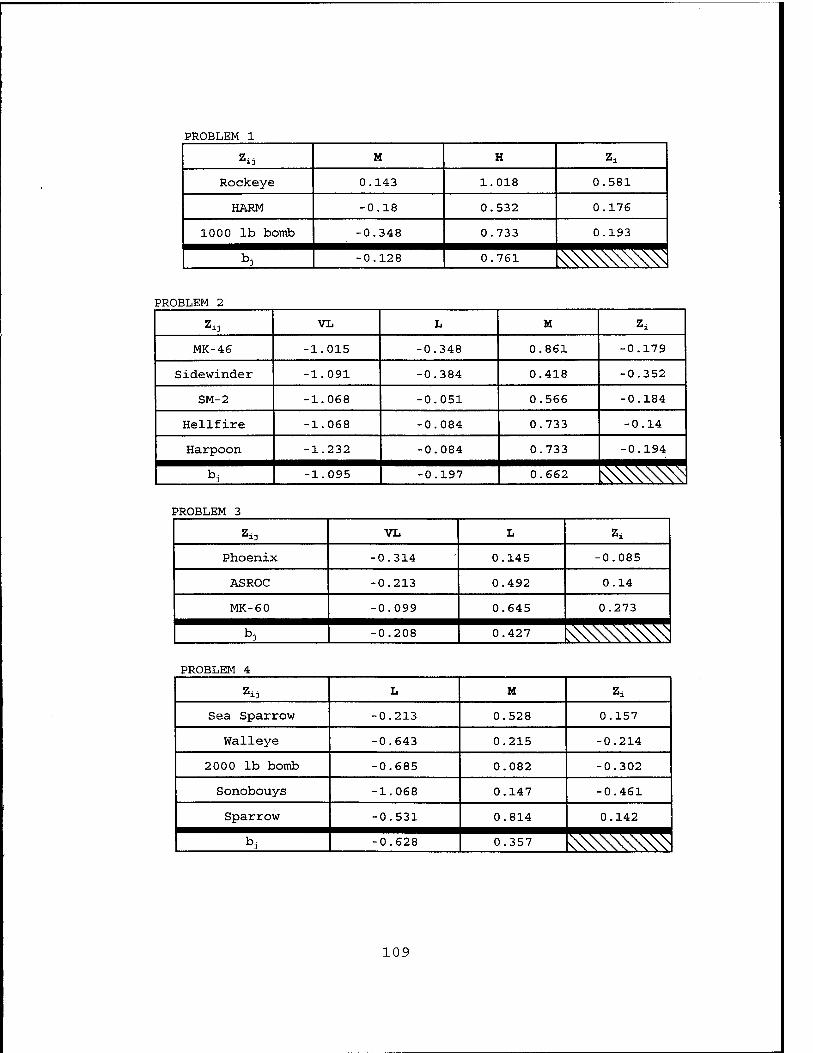
PROBLEM 1
Zi. M H Zi
Rockeye 0.143 1.018 0.581
HARM -0.18 0.532 0.176
1000 lb bomb -0.348 0.733 0.193
*>i -0.128 0.761 mww PROBLEM 2
Zu VL L M Zi
MK-46 -1.015 -0.348 0.861 -0.179
Sidewinder -1.091 -0.384 0.418 -0.352
SM-2 -1.068 -0.051 0.566 -0.184
Hellfire -1.068 -0.084 0.733 -0.14
Harpoon -1.232 -0.084 0.733 -0.194
bj -1.095 -0.197 0.662 M^ PROBLEM 3
Zi3 VL L Zi
Phoenix -0.314 0.145 -0.085
ASROC -0.213 0.492 0.14
MK-60 -0.099 0.645 0.273
*>i -0.208 0.427 wwwww PROBLEM 4
Zii L M Zi
Sea Sparrow -0.213 0.528 0.157
Walleye -0.643 0.215 -0.214
2000 lb bomb -0.685 0.082 -0.302
Sonobouys -1.068 0.147 -0.461
Sparrow -0.531 0.814 0.142
*>j -0.628 0.357 vWWWXW^
109
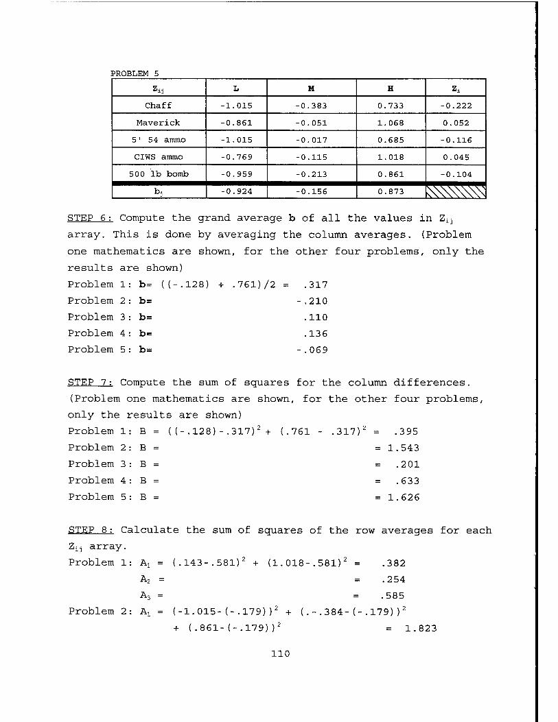
PROBLEM 5
Zi3 L M H Zi
Chaff -1.015 -0.383 0.733 -0.222
Maverick -0.861 -0.051 1.068 0.052
5' 54 ammo -1.015 -0.017 0.685 -0.116
CIWS ammo -0.769 -0.115 1.018 0.045
500 lb bomb -0.959 -0.213 0.861 -0.104
*>J -0.924 -0.156 0.873 ^\\\\\\X STEP 6: Compute the grand average b of all the values in Z±j
array. This is done by averaging the column averages. (Problem
one mathematics are shown, for the other four problems, only the
results are shown)
Problem 1
Problem 2
Problem 3
Problem 4
Problem 5
b= ((-.128) + .76D/2 = .317
b= -.210
b= .110
b= .136
b= -.069
STEP 7: Compute the sum of squares for the column differences.
(Problem one mathematics are shown, for the other four problems,
only the results are shown)
Problem 1
Problem 2
Problem 3
Problem 4
B = ( (-.128)-.317)2 + (.761
B =
B =
B =
Problem 5: B =
.317)2 = .395
= 1.543
= .201
= .633
= 1.626
STEP 8: Calculate the sum of squares of the row averages for each
Zij array.
Problem 1: A1 = (.143-.581)2 + (1.018-.581)2 = .382
A2 =
A3 =
Problem 2: Ax = (-1.015-(-.179))2 +
+ (.861-(-.179))2
.254
.585
384- (-.179))2
= 1.823
110
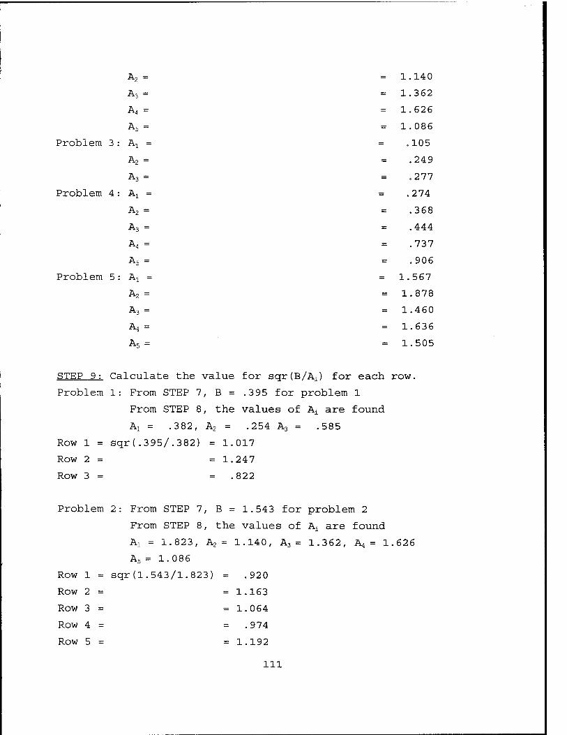
A2 = = 1.140
A3 = = 1.362
A4 = = 1.626
A5 = = 1.086
Problem 3 : Aa = = .105
A2 = = .249
A3 = = .277
Problem 4 : Ax = = .274
A2 = = .368
A3 = = .444
A4 = = .737
A5 = = .906
Problem 5: Ax = = 1.567
A2 = = 1.878
A3 = = 1.460
A4 = = 1.636
A5= = 1.505
STEP 9: Calculate the value for sqr(B/Ai) for each row.
Problem 1: From STEP 7, B = .3 95 for problem 1
From STEP 8, the values of A± are found
Ai = .382, A2 = .254 A3 = .585
Row 1 = sqr(.395/.382) = 1.017
Row 2 = = 1.247
Row 3 = = 822
Problem 2: From STEP 7, B = 1.543 for problem 2
From STEP 8, the values of Ax are found
Ax = 1.823, A2 = 1.140, A3 = 1.362, A4 = 1.626
A5 = 1.086
Row 1 = sqr(1.543/1.823) = .920
Row 2 = = 1.163
Row 3 = = 1.064
Row 4 = = .974
Row 5 = = 1.192
111
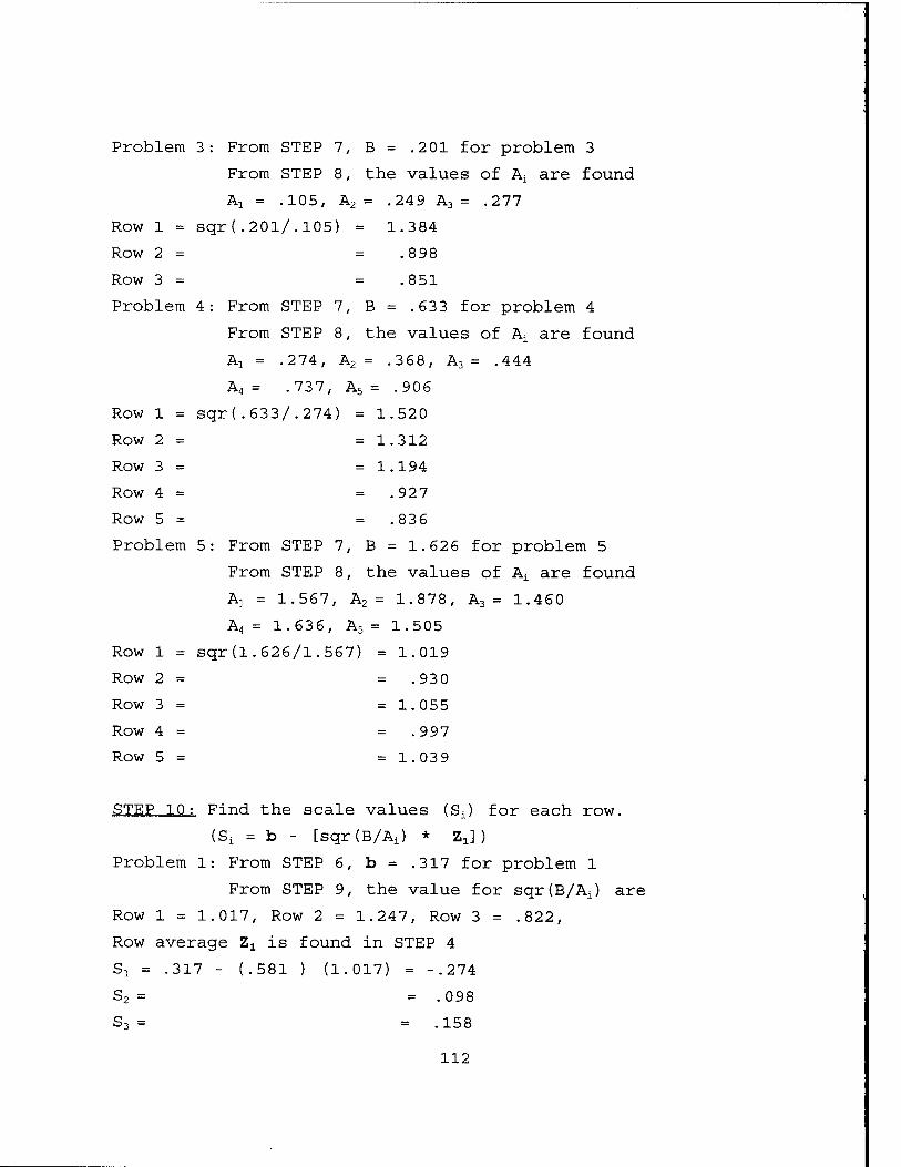
Problem 3: From STEP 7, B = .201 for problem 3
From STEP 8, the values of Ai are found
Al = .105, A2 = .249 A3 = .277
Row 1 = sqr(.20l/.105) = 1.384
Row 2 = .898
Row 3 = .851
Problem 4: From STEP 7, B = .633 for problem 4
From STEP 8, the values of Ai are found
A1 = .274, A2 = .368, A3 = . 444
A4 = .737, A .5 = .906
Row 1 = sqr(.633/.274) = 1.520
Row 2 = = 1.312
Row 3 = = 1.194
Row 4 = = .927
Row 5 = = .836
Problem 5: From STEP 7, B = 1.626 for problem 5
From STEP 8, the values of Ai are found
A1 = 1.567, A2 = 1.878, A3 = 1.460
A4 = 1.63 6, £ L5 = 1.505
Row 1 = sqr(1.626/1.567) = 1.019
Row 2 = = .930
Row 3 = = 1.055
Row 4 = = .997
Row 5 = = 1.039
STEP : LO : Find the scale values (Si) for each row.
(Si = b - [sqr (B/Ai) * ZJ )
Problem 1: From STEP 6, b = .317 for problem 1
From STEP 9, the value for sqr (B/Ai) are ,
Row 1 = 1.017, Row 2 = 1.247, Row 3 = .822,
Row average Zx is found in STEP 4
S1 = • 317 - (.581 ) (1. 317) = -.274
S2 = = .098
S3 = = .158
112
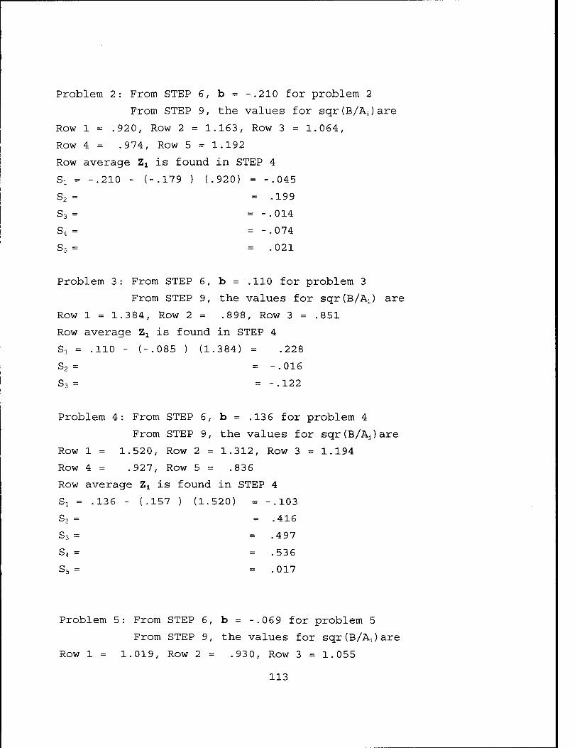
Problem 2: From STEP 6, b = -.210 for problem 2
From STEP 9, the values for sqr(B/Ai)are
Row 1 = .920, Row 2=1 .163, Row 3 = 1.064,
Row 4 = .974, Row 5 = 1.192
Row average Zx is found in STEP 4
Si = -.210 - (-.179 ) (. 920) = -.045
S2 = = .199
s3 = = -.014
s4 = = -.074
s5 = = .021
Problem 3: From STEP 6, b = .110 for problem 3
From STEP 9, the values for sqr(B/Ai) are
Row 1 = 1.3 84, Row 2 = .898, Row 3 = .851
Row average Zx is found in STEP 4
S1 = .110 - (-.085 ) (1 384) = .228
S2 = = -.016
S3 = = -.122
Problem 4: From STEP 6, b = .136 for problem 4
From STEP 9, the values for sqr(B/Ai)are
Row 1 = 1.520, Row 2 = 1.312, Row 3 = 1.194
Row 4 = .927, Row 5 = .836
Row average Zx is found in STEP 4
Si = .136 - (.157 ) (1.! 520) = -.103
S2 = = .416
S3 = = .497
S4 = = .536
s5 = = .017
Problem 5: From STEP 6, b = -.069 for problem 5
From STEP 9, the values for sqr(B/A±)are
Row 1 = 1.019, Row 2 = .930, Row 3 = 1.055
113
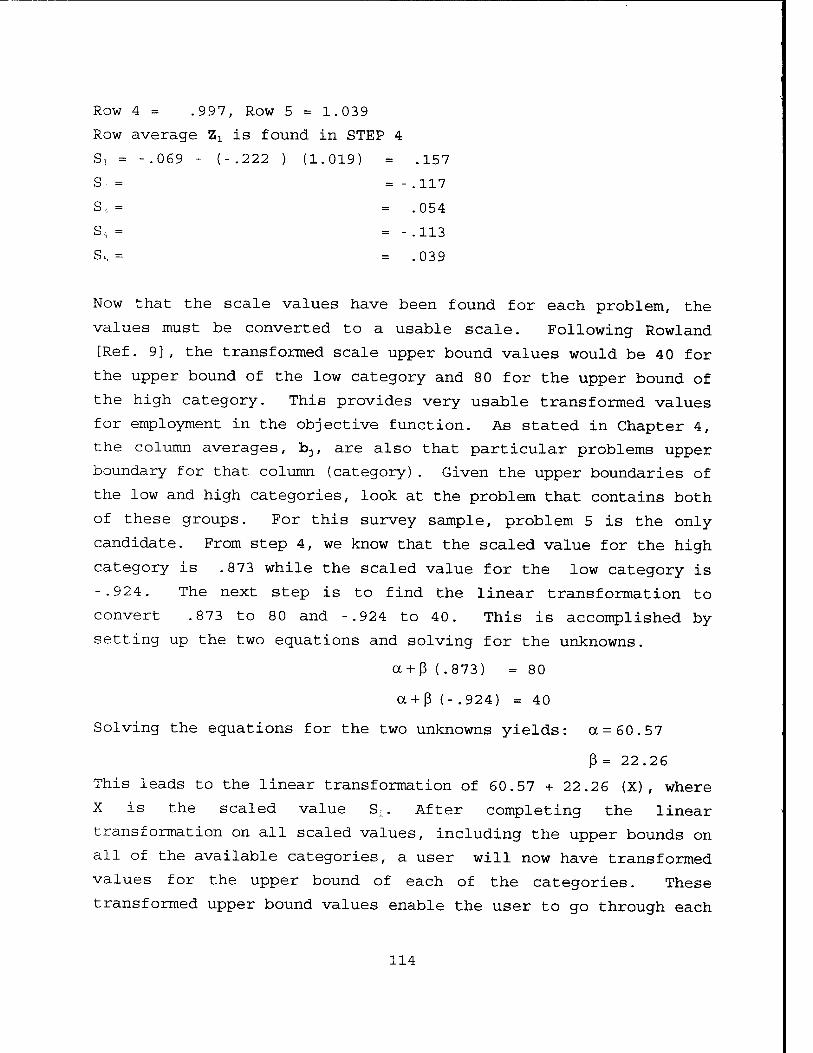
Row 4 = .997, Row 5 = 1.039
Row average Zx is found in STEP 4
S, = -.069 - (-.222 ) (1.019) = .157
S = = - .117
S, = = .054
S, = = -.113
S, = = .039
Now that the scale values have been found for each problem, the
values must be converted to a usable scale. Following Rowland
[Ref. 9], the transformed scale upper bound values would be 40 for
the upper bound of the low category and 80 for the upper bound of
the high category. This provides very usable transformed values
for employment in the objective function. As stated in Chapter 4,
the column averages, b3, are also that particular problems upper
boundary for that column (category). Given the upper boundaries of
the low and high categories, look at the problem that contains both
of these groups. For this survey sample, problem 5 is the only
candidate. From step 4, we know that the scaled value for the high
category is .873 while the scaled value for the low category is
-.924. The next step is to find the linear transformation to
convert .873 to 80 and -.924 to 40. This is accomplished by
setting up the two equations and solving for the unknowns.
oc + ß (.873) = 80
a + ß (- .924) = 40
Solving the equations for the two unknowns yields: a =60.57
ß = 22.26
This leads to the linear transformation of 60.57 + 22.26 (X), where
X is the scaled value SL. After completing the linear
transformation on all scaled values, including the upper bounds on
all of the available categories, a user will now have transformed
values for the upper bound of each of the categories. These
transformed upper bound values enable the user to go through each
114
of the remaining problems and transform the scaled values. The
following are the linear transformations used in the five problems:
Problem 1
Problem 2
Problem 3
Problem 4
Problem 5
60.40 + 25.76 (X)
43.92 + 19.91 (X)
28.00 + 28.20 (X)
50.90 + 17.40 (X)
60.57 + 22.26 (X)
Table 16 in Chapter IV shows the final transformed results.
115
116
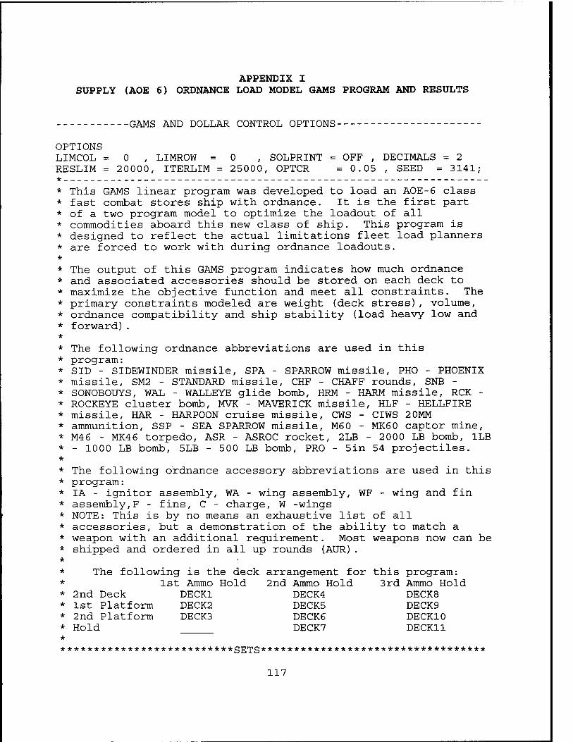
APPENDIX I SUPPLY (AOE 6) ORDNANCE LOAD MODEL GAMS PROGRAM AND RESULTS
-GAMS AND DOLLAR CONTROL OPTIONS-
OPTIONS LIMCOL = 0 , LIMROW = 0 , SOLPRINT = OFF , DECIMALS = 2 RESLIM = 20000, ITERLIM = 25000, OPTCR = 0.05 , SEED = 3141; *
* This GAMS linear program was developed to load an AOE-6 class * fast combat stores ship with ordnance. It is the first part * of a two program model to optimize the loadout of all * commodities aboard this new class of ship. This program is * designed to reflect the actual limitations fleet load planners * are forced to work with during ordnance loadouts. *
* The output of this GAMS program indicates how much ordnance * and associated accessories should be stored on each deck to * maximize the objective function and meet all constraints. The * primary constraints modeled are weight (deck stress), volume, * ordnance compatibility and ship stability (load heavy low and * forward). *
* The following ordnance abbreviations are used in this * program: * SID - SIDEWINDER missile, SPA - SPARROW missile, PHO - PHOENIX * missile, SM2 - STANDARD missile, CHF - CHAFF rounds, SNB - * SONOBOUYS, WAL - WALLEYE glide bomb, HRM - HARM missile, RCK - * ROCKEYE cluster bomb, MVK - MAVERICK missile, HLF - HELLFIRE * missile, HAR - HARPOON cruise missile, CWS - CIWS 20MM * ammunition, SSP - SEA SPARROW missile, M60 - MK60 captor mine, * M46 - MK46 torpedo, ASR - ASROC rocket, 2LB - 2000 LB bomb, 1LB * - 1000 LB bomb, 5LB - 500 LB bomb, PRO - 5in 54 projectiles. *
* The following ordnance accessory abbreviations are used in this * program: * IA - ignitor assembly, WA - wing assembly, WF - wing and fin * assembly,F - fins, C - charge, W -wings * NOTE: This is by no means an exhaustive list of all * accessories, but a demonstration of the ability to match a * weapon with an additional requirement. Most weapons now can be * shipped and ordered in all up rounds (AUR). *
* The following is the deck arrangement for this program: * 1st Ammo Hold 2nd Ammo Hold 3rd Ammo Hold * 2nd Deck DECK1 DECK4 DECK8 * 1st Platform DECK2 DECK5 DECK9 * 2nd Platform DECK3 DECK6 DECK10 * Hold DECK7 DECK11 * ************************** SETS **********************************
117
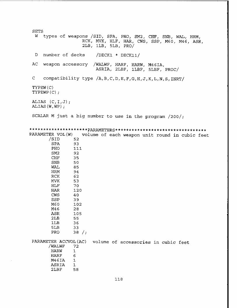
SETS W types of weapons /SID, SPA, PHO, SM2, CHF, SNB, WAL, HRM,
RCK, MVK, HLF, HAR, CWS, SSP, M60, M46, ASR, 2LB, 1LB, 5LB, PRO/
D number of decks /DECK1 * DECKll/
AC weapon accessory /WALWF, HARF, HARW, M46IA, ASRIA, 2LBF, 1LBF, 5LBF, PROC/
C compatibility type /A,B,C,D,E,F,G,H,J,K,L,N,S,INRT/
TYPEW(C) TYPEWP(C);
ALIAS (C,I,J); ALIAS(W,WP);
SCALAR M just a big number to use in the program /2 00/;
********************* PARAMETERS ********************************* PARAMETER VOL(W) volume of each weapon unit round in cubic feet
/SID 52 SPA 93 PHO 111 SM2 92 CHF 35 SNB 50 WAL 85 HRM 94 RCK 62 MVK 53 HLF 70 HAR 120 CWS 40 SSP 39 M6 0 102 M46 28 ASR 105 2 LB 55 1LB 36 5 LB 33 PRO 38 /;
PARAMETER ACCVOL(AC) /WALWF 72 HARW 1 HARF 6 M4 6IA 1 ASRIA 1 2LBF 58
volume of accessories in cubic feet
118
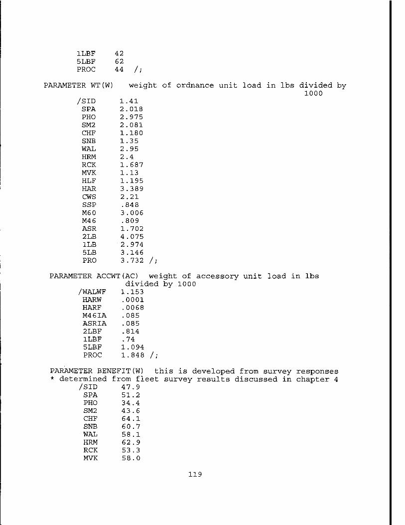
1LBF 42 5LBF 62 PROC 44 /;
A.RAMETER WT (W) weight of ordnance unit load in lbs divided by 1000
/SID 1.41 SPA 2.018 PHO 2.975 SM2 2.081 CHF 1.180 SNB 1.35 WAL 2.95 HRM 2.4 RCK 1.687 MVK 1.13 HLF 1.195 HAR 3.389 CWS 2.21 SSP .848 M60 3.006 M46 .809 ASR 1.702 2 LB 4.075 1LB 2.974 5 LB 3.146 PRO 3.732 /;
PARAMETER ACCWT(AC) weight of accessory unit load in lbs divided by 1000
/WALWF 1.153 HARW .0001 HARF .0068 M46IA .085 ASRIA .085 2LBF .814 1LBF .74 5LBF 1.094 PROC 1.848 /;
PARAMETER BENEFIT(W) this is developed from survey responses * determined from fleet survey results discussed in chapter 4
/SID 47 9 SPA 51 2 PHO 34 4 SM2 43 6 CHF 64 1 SNB 60 7 WAL 58 1 HRM 62 .9 RCK 53 .3 MVK 58 .0
119
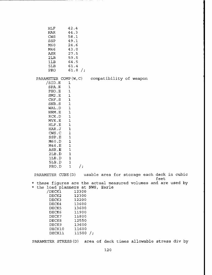
HLF 42.4 HAR 44.3 CWS 58.1 SSP 49.1 M60 24.6 M46 43.0 ASR 27.5 2 LB 59.5 1LB 64.5 5 LB 61.4 PRO 61.8 /
PARAMETER COMP(W,C) /SID.E 1 SPA.E 1 PHO.E 1 SM2.E 1 CHF.S 1 SNB.S 1 WAL.D 1 HRM.E 1 RCK.D 1 MVK.E 1 HLF.E 1 HAR. J 1 CWS.C 1 SSP.E 1 M60.D 1 M46.E 1 ASR.E 1 2LB.D 1 1LB.D 1 5LB.D 1 PRO.D 1 /
compatibility of weapon
PARAMETER CUBE(D) usable area for storage each deck in cubic feet
* these figures are the actual measured volumes and are used by * the load planners at NWS, Earle
DECK1 12300 DECK2 12300 DECK3 12200 DECK4 13600 DECK5 13600 DECK6 11900 DECK7 11800 DECK8 12550 DECK9 13600 DECK10 11600 DECK11 11500 /;
PARAMETER STRESS(D) area of deck times allowable stress div by
120
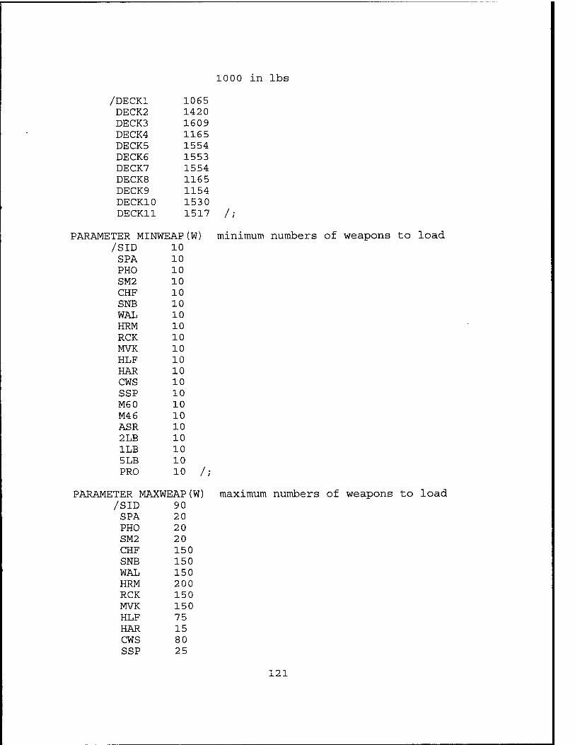
1000 in lbs
/DECK1 1065 DECK2 1420 DECK3 1609 DECK4 1165 DECK5 1554 DECK6 1553 DECK7 1554 DECK8 1165 DECK9 1154 DECK10 1530 DECK11 1517
TER MINWEAP(W) /SID 10 SPA 10 PHO 10 SM2 10 CHF 10 SNB 10 WAL 10 HRM 10 RCK 10 MVK 10 HLF 10 HAR 10 CWS 10 SSP 10 M60 10 M46 10 ASR 10 2 LB 10 1LB 10 5 LB 10 PRO 10 /;
3TER MAXWEAP(W) /SID 90 SPA 20 PHO 20 SM2 20 CHF 150 SNB 150 WAL 150 HRM 200 RCK 150 MVK 150 HLF 75 HAR 15 CWS 80 SSP 25
/;
minimum numbers of weapons to load
maximum numbers of weapons to load
121
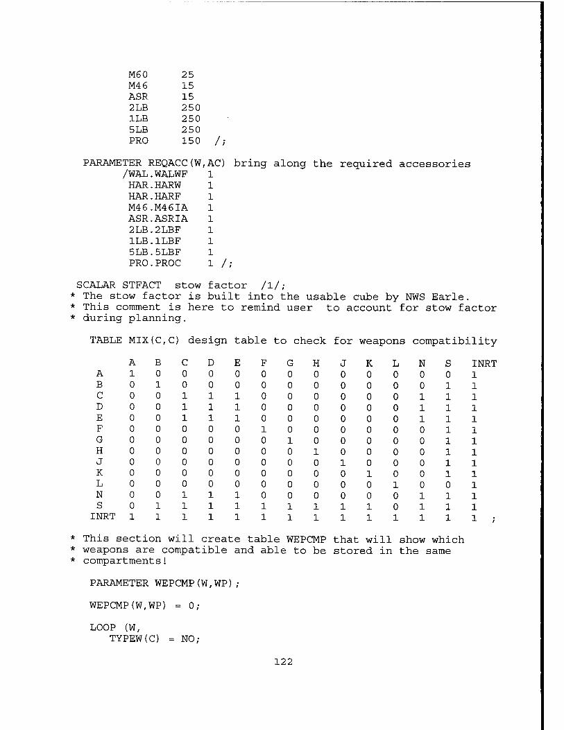
M60 25 M46 15 ASR 15 2LB 250 1LB 250 5LB 250 PRO 150 /;
PARAMETER REQACC(W,AC) bring along the required accessories /WAL.WALWF 1 HAR.HARW 1 HAR.HARF 1 M46.M46IA 1 ASR.ASRIA 1 2LB.2LBF 1 1LB.1LBF 1 5LB.5LBF 1 PRO.PROC 1 /;
SCALAR STFACT stow factor /l/; * The stow factor is built into the usable cube by NWS Earle. * This comment is here to remind user to account for stow factor * during planning.
TABLE MIX(C,C) design table to check for weapons compatibility
ABCDEFGHJKLNS INRT A 1 0 0 0 0 0 0 0 0 0 0 0 0 1 B 0 1 0 0 0 0 0 0 0 0 0 0 1 1 C 0 0 1 1 1 0 0 0 0 0 0 1 1 1 D 0 0 1 1 1 0 0 0 0 0 0 1 1 1 E 0 0 1 1 1 0 0 0 0 0 0 1 1 1 F 0 0 0 0 0 1 0 0 0 0 0 0 1 1 G 0 0 0 0 0 0 1 0 0 0 0 0 1 1 H 0 0 0 0 0 0 0 1 0 0 0 0 1 1 J 0 0 0 0 0 0 0 0 1 0 0 0 1 1 K 0 0 0 0 0 0 0 0 0 1 0 0 1 1 L 0 0 0 0 0 0 0 0 0 0 1 0 0 1 N 0 0 1 1 1 0 0 0 0 0 0 1 1 1 S 0 1 1 1 1 1 1 1 1 1 0 1 1 1 INRT 1111111111111
* This section will create table WEPCMP that will show which * weapons are compatible and able to be stored in the same * compartments!
PARAMETER WEPCMP(W,WP);
WEPCMP(W,WP) = 0;
LOOP (W, TYPEW(C) = NO;
122
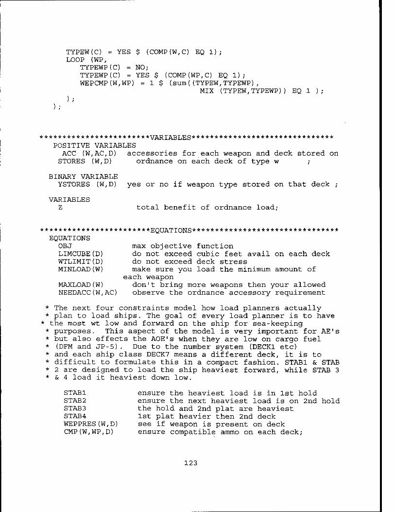
TYPEW(C) = YES $ (COMP(W,C) EQ 1); LOOP (WP,
TYPEWP(C) = NO; TYPEWP(C) = YES $ (COMP(WP,C) EQ 1); WEPCMP(W,WP) = 1 $ (sum((TYPEW,TYPEWP),
MIX (TYPEW,TYPEWP)) EQ 1 ); );
);
************************VARIABLES******************************* POSITIVE VARIABLES ACC (W,AC,D) accessories for each weapon and deck stored on STORES (W,D) ordnance on each deck of type w ;
BINARY VARIABLE YSTORES (W,D) yes or no if weapon type stored on that deck ;
VARIABLES Z total benefit of ordnance load;
************************EQUATIONS******************************** EQUATIONS
OBJ max objective function LIMCUBE(D) do not exceed cubic feet avail on each deck WTLIMIT(D) do not exceed deck stress MINLOAD(W) make sure you load the minimum amount of
each weapon MAXLOAD(W) don't bring more weapons then your allowed NEEDACC(W,AC) observe the ordnance accessory requirement
* The next four constraints model how load planners actually * plan to load ships. The goal of every load planner is to have
* the most wt low and forward on the ship for sea-keeping * purposes. This aspect of the model is very important for AE's * but also effects the AOE's when they are low on cargo fuel * (DFM and JP-5). Due to the number system (DECK1 etc) * and each ship class DECK7 means a different deck, it is to * difficult to formulate this in a compact fashion. STAB1 & STAB * 2 are designed to load the ship heaviest forward, while STAB 3 * & 4 load it heaviest down low.
STAB1 ensure the heaviest load is in 1st hold STAB2 ensure the next heaviest load is on 2nd hold STAB3 the hold and 2nd plat are heaviest STAB4 1st plat heavier then 2nd deck WEPPRES(W,D) see if weapon is present on deck CMP(W,WP,D) ensure compatible ammo on each deck;
123
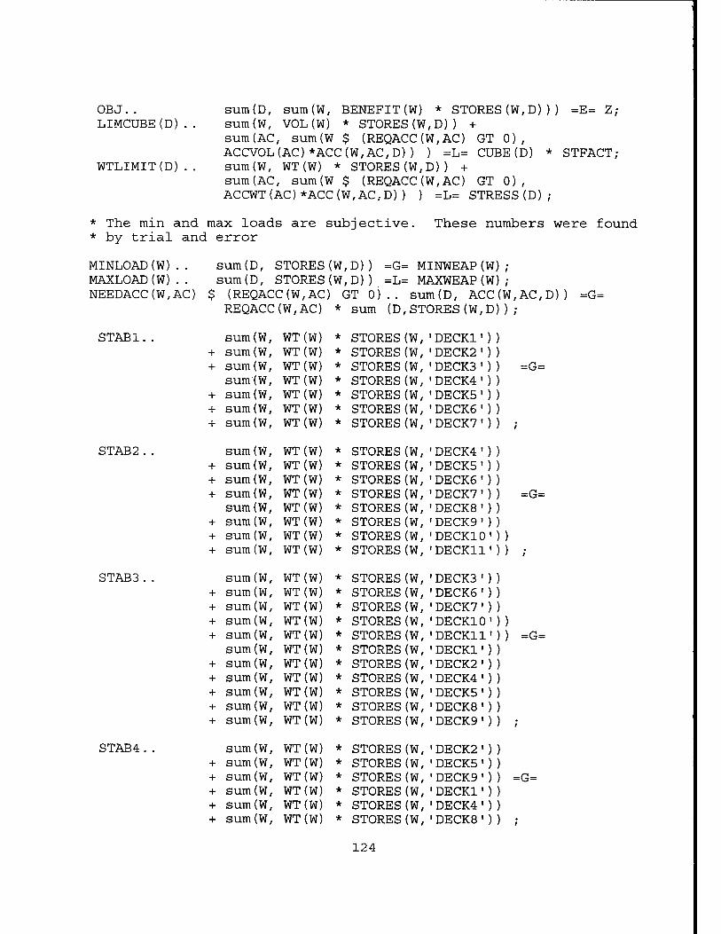
OBJ. . LIMCUBE(D)..
WTLIMIT(D).
sum(D, sum(W, BENEFIT(W) * STORES(W,D))) =E= Z; sum(W, VOL(W) * STORES(W,D)) + sum(AC, sum(W $ (REQACC(W,AC) GT 0), ACCVOL(AC)*ACC(W,AC,D)) ) =L= CUBE(D) * STFACT; sum(W, WT(W) * STORES(W,D)) + sum(AC, sum(W $ (REQACC(W,AC) GT 0), ACCWT(AC)*ACC(W,AC,D)) ) =L= STRESS(D);
* The min and max loads are subjective. * by trial and error
These numbers were found
MINLOAD(W).. MAXLOAD(W).. NEEDACC(W,AC)
STAB1
STAB2
STAB 3
STAB4
sum(D, STORES(W,D)) =G= MINWEAP(W sum(D, STORES(W,D)) =L= MAXWEAP(W
$ (REQACC(W,AC) GT 0).. sum(D, ACC REQACC(W,AC) * sum (D,STORES(W,D
+ +
+ + +
+ + +
+ + +
+ + + +
+ + + +
+ + + + +
sum( w, WT (W) sum ( W WT (w) sum( W WT (W) sum ( W WT (W) sum W WT (W) sum! W WT (W) sum! W WT (W)
sum( W WT (W) sum! W WT (w) sum W WT (W) sum ( W WT (w) sum( W WT (W) sum W WT (w) sum W WT (W) sum W WT (W)
sum W WT (w) sum W WT (w) sum W WT (w) sum W WT (w) sum W , WT (W) sum w , WT (w) sum w , WT (w) sum w , WT (W) sum w , WT (w) sum w , WT (w) sum w , WT (w)
sum w , WT (W) sum w , WT (w) sum iW , WT (w) sum
fw , WT (W) sum w , WT (W) sum kw , WT (w)
* * * * * * *
* * * * * * * *
* * * * * * * * * * *
* * * * * *
STORES (W, STORES (W, STORES (W STORES (W STORES (W STORES (W STORES (W
STORES (W STORES (W STORES (W STORES (W STORES (W STORES (W STORES (W STORES (W
STORES (W STORES (W STORES (W STORES (W STORES (W STORES (W STORES (w STORES (w STORES (W STORES (w STORES (w
STORES (w STORES (w STORES (w STORES (W STORES (w STORES (w
DECK1 DECK2 DECK3 DECK4 DECK5 DECK6 DECK7
DECK4 DECK5 DECK6 DECK7 DECK8 DECK9 DECK10* DECK11*
DECK3') DECK6') DECK7■) DECK10' DECK11' DECK1 DECK2 DECK4 DECK5 DECK8 DECK9
DECK2 DECK5 DECK9 DECK1 DECK4 DECK8
W,AC,D)) );
=G=
=G=
=G=
) =G=
=G=
124
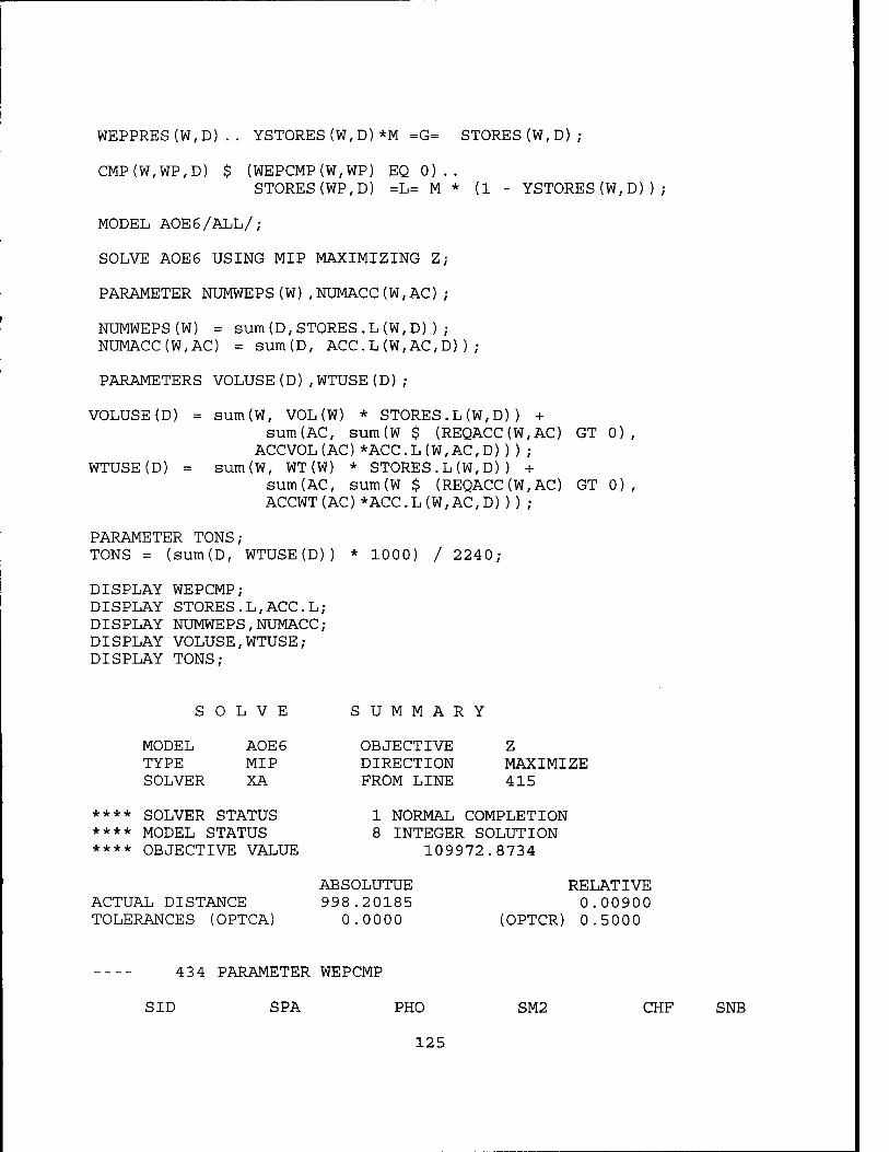
WEPPRES(W,D).. YSTORES(W,D)*M =G= STORES(W,D);
$ (WEPCMP(W,WP) EQ 0).. YSTORES(W,D));
CMP(W,WP,D) $ (WEPCMP(W,WP) EQ 0).. STORES(WP,D) =L= M * (1
MODEL AOE6/ALL/;
SOLVE AOE6 USING MIP MAXIMIZING Z
PARAMETER NUMWEPS(W),NUMACC(W,AC)
NUMWEPS(W) = sum(D,STORES.L(W,D)) NUMACC(W,AC) = sum(D, ACC.L(W,AC,D));
PARAMETERS VOLUSE(D),WTUSE(D);
VOLUSE(D) = sum(W, VOL(W) * STORES.L(W,D)) + sum(AC, sum(W $ (REQACC(W,AC) GT 0),
ACCVOL(AC)*ACC.L(W,AC,D))); WTUSE(D) = sum(W, WT(W) * STORES.L(W,D)) +
sum(AC, sum(W $ (REQACC(W,AC) GT 0), ACCWT(AC)*ACC.L(W,AC,D)));
PARAMETER TONS; TONS = (sura(D, WTUSE(D)) * 1000) / 2240;
DISPLAY WEPCMP; DISPLAY STORES.L,ACC.L; DISPLAY NUMWEPS,NUMACC; DISPLAY VOLUSE,WTUSE; DISPLAY TONS;
SOLVE
MODEL AOE6 TYPE MIP SOLVER XA
**** SOLVER STATUS **** MODEL STATUS **** OBJECTIVE VALUE
ACTUAL DISTANCE TOLERANCES (OPTCA)
SUMMARY
OBJECTIVE DIRECTION FROM LINE
MAXIMIZE 415
1 NORMAL COMPLETION 8 INTEGER SOLUTION
109972.8734
ABSOLUTUE 998.20185
0.0000
RELATIVE 0.00900
(OPTCR) 0.5000
434 PARAMETER WEPCMP
SID SPA PHO
125
SM2 CHF SNB
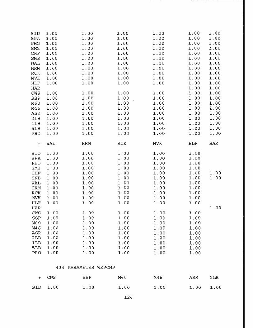
SID 1.00 1.00 1.00 1.00 1.00 1.00 SPA 1.00 1.00 1.00 1.00 1.00 1.00 PHO 1.00 1.00 1.00 1.00 1.00 1.00 SM2 1.00 1.00 1.00 1.00 1.00 1.00 CHF 1.00 1.00 1.00 1.00 1.00 1.00 SNB 1.00 1.00 1.00 1.00 1.00 1.00 WAL 1.00 1.00 1.00 1.00 1.00 1.00 HRM 1.00 1.00 1.00 1.00 1.00 1.00 RCK 1.00 1.00 1.00 1.00 1.00 1.00 MVK 1.00 1.00 1.00 1.00 1.00 1.00 HLF 1.00 1.00 1.00 1.00 1.00 1.00 HAR 1.00 1.00 CWS 1.00 1.00 1.00 1.00 1.00 1.00 SSP 1.00 1.00 1.00 1.00 1.00 1.00 M60 1.00 1.00 1.00 1.00 1.00 1.00 M46 1.00 1.00 1.00 1.00 1.00 1.00 ASR 1.00 1.00 1.00 1.00 1.00 1.00 2 LB 1.00 1.00 1.00 1.00 1.00 1.00 1LB 1.00 1.00 1.00 1.00 1.00 1.00 5 LB 1.00 1.00 1.00 1.00 1.00 1.00 PRO 1.00 1.00 1.00 1.00 1.00 1.00
WAL HRM RCK MVK HLF HAR
SID 1.00 1.00 1.00 1.00 1.00 SPA 1.00 1.00 1.00 1.00 1.00 PHO 1.00 1.00 1.00 1.00 1.00 SM2 1.00 1.00 1.00 1.00 1.00 CHF 1.00 1.00 1.00 1.00 1.00 1.00 SNB 1.00 1.00 1.00 1.00 1.00 1.00 WAL 1.00 1.00 1.00 1.00 1.00 HRM 1.00 1.00 1.00 1.00 1.00 RCK 1.00 1.00 1.00 1.00 1.00 MVK 1.00 1.00 1.00 1.00 1.00 HLF 1.00 1.00 1.00 1.00 1.00 HAR 1.00 CWS 1.00 1.00 1.00 1.00 1.00 SSP 1.00 1.00 1.00 1.00 1.00 M60 1.00 1.00 1.00 1.00 1.00 M4 6 1.00 1.00 1.00 1.00 1.00 ASR 1.00 1.00 1.00 1.00 1.00 2 LB 1.00 1.00 1.00 1.00 1.00 1LB 1.00 1.00 1.00 1.00 1.00 5 LB 1.00 1.00 1.00 1.00 1.00 PRO 1.00 1.00 1.00 1.00 1.00
434 PARAMETER WEPCMP
+ CWS SSP M60
SID 1.00 1.00 1.00
126
M4 6
1.00
ASR 2LB
1.00 1.00
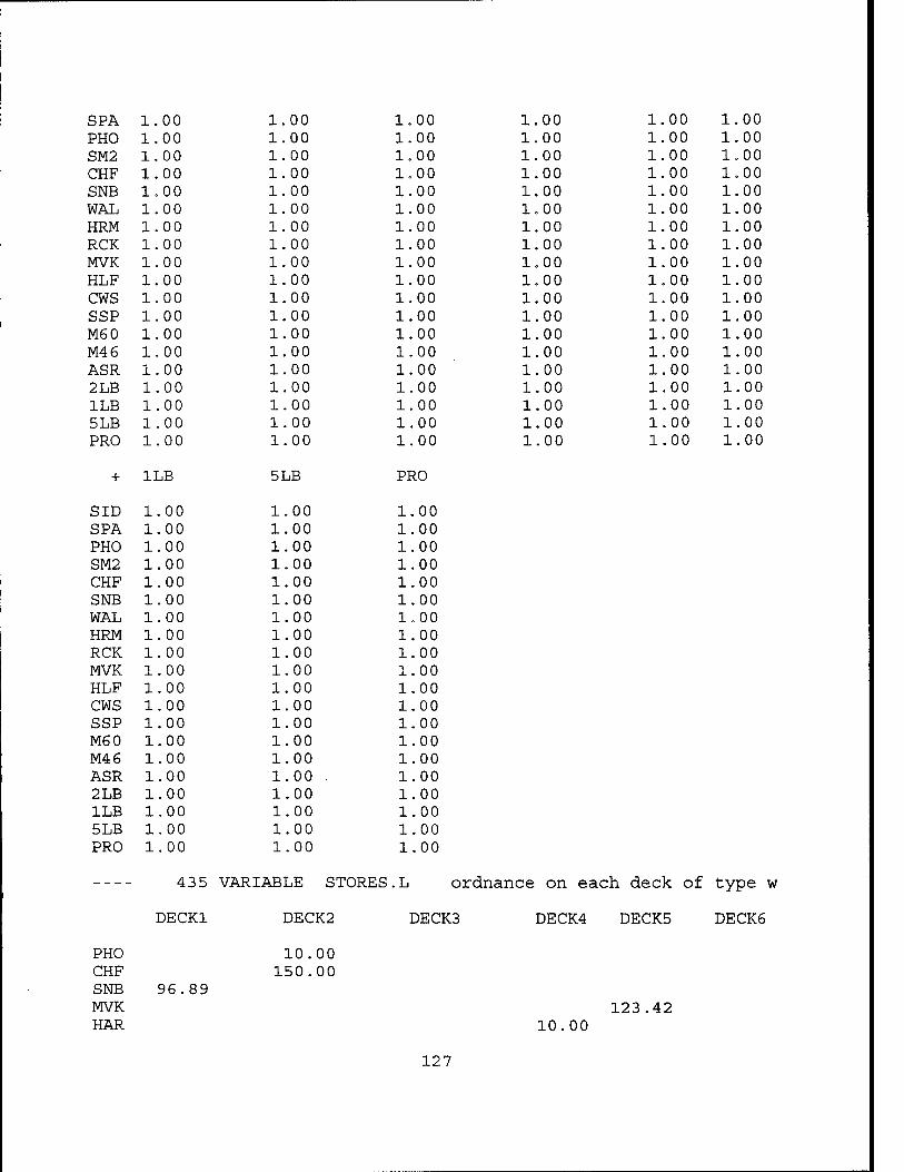
SPA 1.00 1.00 1.00 1.00 1.00 1.00 PHO 1.00 1.00 1.00 1.00 1.00 1.00 SM2 1.00 1.00 1.00 1.00 1.00 1.00 CHF 1.00 1.00 1.00 1.00 1.00 1.00 SNB 1.00 1.00 1.00 1.00 1.00 1.00 WAL 1.00 1.00 1.00 1.00 1.00 1.00 HRM 1.00 1.00 1.00 1.00 1.00 1.00 RCK 1.00 1.00 1.00 1.00 1.00 1.00 MVK 1.00 1.00 1.00 1.00 1.00 1.00 HLF 1.00 1.00 1.00 1.00 1.00 1.00 CWS 1.00 1.00 1.00 1.00 1.00 1.00 SSP 1.00 1.00 1.00 1.00 1.00 1.00 M60 1.00 1.00 1.00 1.00 1.00 1.00 M46 1.00 1.00 1.00 1.00 1.00 1.00 ASR 1.00 1.00 1.00 1.00 1.00 1.00 2 LB 1.00 1.00 1.00 1.00 1.00 1.00 1LB 1.00 1.00 1.00 1.00 1.00 1.00 5 LB 1.00 1.00 1.00 1.00 1.00 1.00 PRO 1.00 1.00 1.00 1.00 1.00 1.00
1LB 5LB PRO
SID 1.00 1.00 1.00 SPA 1.00 1.00 1.00 PHO 1.00 1.00 1.00 SM2 1.00 1.00 1.00 CHF 1.00 1.00 1.00 SNB 1.00 1.00 1.00 WAL 1.00 1.00 1.00 HRM 1.00 1.00 1.00 RCK 1.00 1.00 1.00 MVK 1.00 1.00 1.00 HLF 1.00 1.00 1.00 CWS 1.00 1.00 1.00 SSP 1.00 1.00 1.00 M60 1.00 1.00 1.00 M46 1.00 1.00 1.00 ASR 1.00 1.00 1.00 2 LB 1.00 1.00 1.00 1LB 1.00 1.00 1.00 5 LB 1.00 1.00 1.00 PRO 1.00 1.00 1.00
43 5 VARIABLE STORES.L ordnance on each deck of type w
DECK1 DECK2 DECK3 DECK4 DECK5 DECK6
PHO 10.00 CHF 150.00 SNB MWCf
96.89
HAR 123.42
10.00
127
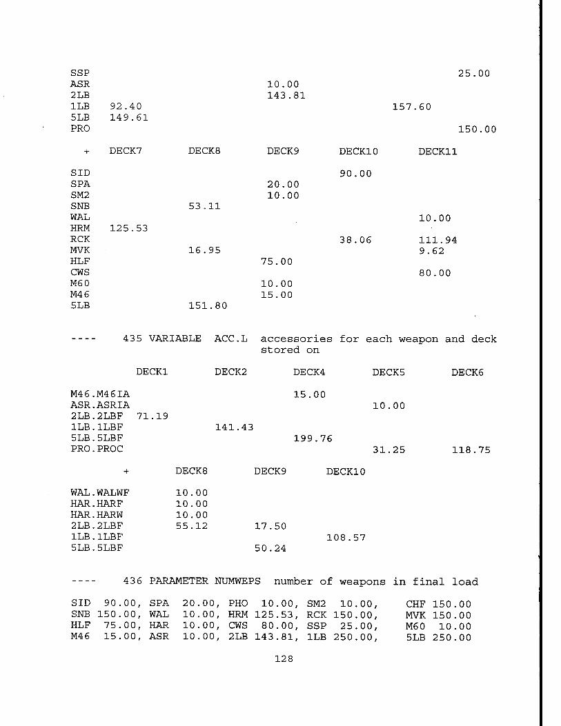
2 LB 1LB 92.40 5 LB 149.61 PRO
25.00
SID SPA SM2 SNB WAL HRM RCK MVK HLF CWS M60 M46 5 LB
DECK7
125.53
DECK8
53.11
16.95
10.00 143.81
DECK9
20.00 10.00
75.00
10.00 15.00
157.60
DECK10 DECK11
90.00
10.00
38.06
150.00
111.94 9.62
80.00
151.80
435 VARIABLE ACC.L accessories for each weapon and deck stored on
DECK1
M46.M46IA ASR.ASRIA 2LB.2LBF 71.19 1LB.1LBF 5LB.5LBF PRO.PROC
DECK2
141.43
DECK4
15.00
199.76
DECK5
10.00
31.25
DECK6
118.75
DECK8 DECK9 DECK10
WAL.WALWF 10.00 HAR.HARF 10.00 HAR.HARW 10.00 2LB.2LBF 55.12 17.50 1LB.1LBF 108.57 5LB.5LBF 50.24
436 PARAMETER NUMWEPS number of weapons in final load
SID 90 00, SPA 20 00, PHO 10 00, SM2 10 00, CHF 150 00 SNB 150 00, WAL 10 00, HRM 125 53, RCK 150 00, MVK 150 00 HLF 75 00, HAR 10 00, CWS 80 00, SSP 25 00, M60 10 00 M4 6 15 00, ASR 10 00, 2 LB 143 81, 1LB 250 00, 5 LB 250 00
128
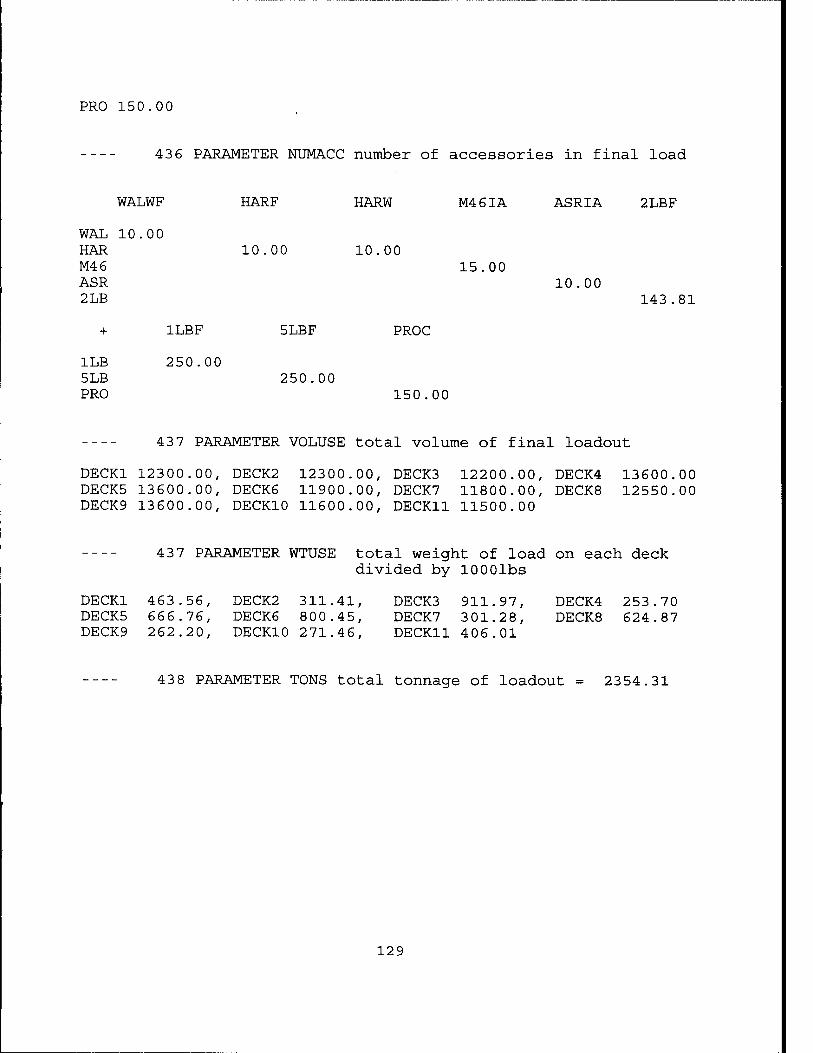
PRO 150.00
436 PARAMETER NUMACC number of accessories in final load
WALWF HARF HARW M46IA ASRIA 2LBF
15.00 10.00
143.81
WAL HAR M46 ASR 2 LB
10 00 10.00 10.00
+ 1LBF 5LBF PROC
ILB 5 LB PRO
250.00 250.00
150.00
437 PARAMETER VOLUSE total volume of final loadout
DECK1 12300.00, DECK2 12300.00, DECK3 12200.00, DECK4 13600.00 DECK5 13600.00, DECK6 11900.00, DECK7 11800.00, DECK8 12550.00 DECK9 13600.00, DECK10 11600.00, DECK11 11500.00
437 PARAMETER WTUSE total weight of load on each deck divided by lOOOlbs
DECK1 463.56, DECK2 311.41, DECK3 911.97, DECK4 253.70 DECK5 666.76, DECK6 800.45, DECK7 301.28, DECK8 624.87 DECK9 262.20, DECK10 271.46, DECK11 406.01
43 8 PARAMETER TONS total tonnage of loadout = 2354.31
129
130
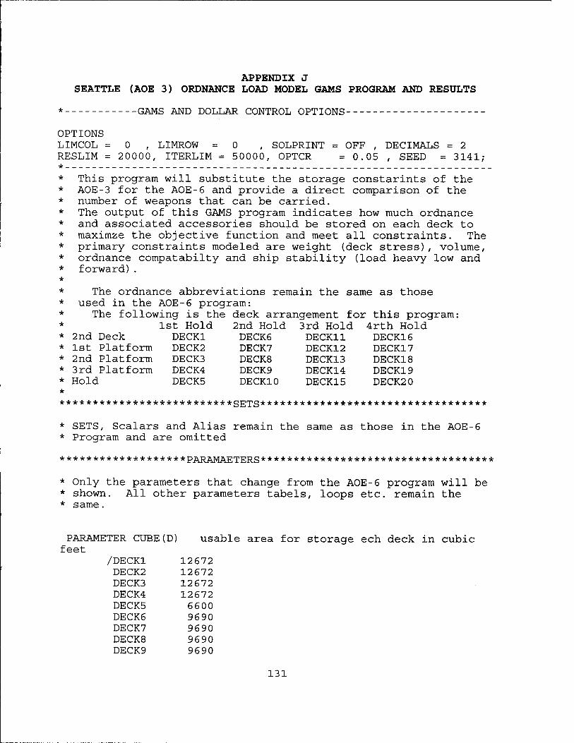
APPENDIX J SEATTLE (AOE 3) ORDNANCE LOAD MODEL GAMS PROGRAM AND RESULTS
* GAMS AND DOLLAR CONTROL OPTIONS
OPTIONS LIMCOL = 0 , LIMROW = 0 , SOLPRINT = OFF , DECIMALS = 2 RESLIM = 20000, ITERLIM = 50000, OPTCR = 0.05 , SEED = 3141; *
* This program will substitute the storage constarints of the * AOE-3 for the AOE-6 and provide a direct comparison of the * number of weapons that can be carried. * The output of this GAMS program indicates how much ordnance * and associated accessories should be stored on each deck to * maximze the objective function and meet all constraints. The * primary constraints modeled are weight (deck stress), volume, * ordnance compatabilty and ship stability (load heavy low and * forward). *
* The ordnance abbreviations remain the same as those * used in the AOE-6 program: * The following is the deck arrangement for this program: * 1st Hold 2nd Hold 3rd Hold 4rth Hold * 2nd Deck DECK1 DECK6 DECK11 DECK16 * 1st Platform DECK2 DECK7 DECK12 DECK17 * 2nd Platform DECK3 DECK8 DECK13 DECK18 * 3rd Platform DECK4 DECK9 DECK14 DECK19 * Hold DECK5 DECK10 DECK15 DECK20 * ************************** SETS **********************************
* SETS, Scalars and Alias remain the same as those in the AOE-6 * Program and are omitted
******************* PARAMAETERS ***********************************
* Only the parameters that change from the AOE-6 program will be * shown. All other parameters tabels, loops etc. remain the * same.
usable area for storage ech deck in cubic PARAMETER CUBE(D) us feet
/DECK1 12672 DECK2 12672 DECK3 12672 DECK4 12672 DECK5 6600 DECK6 9690 DECK7 9690 DECK8 9690 DECK9 9690
131
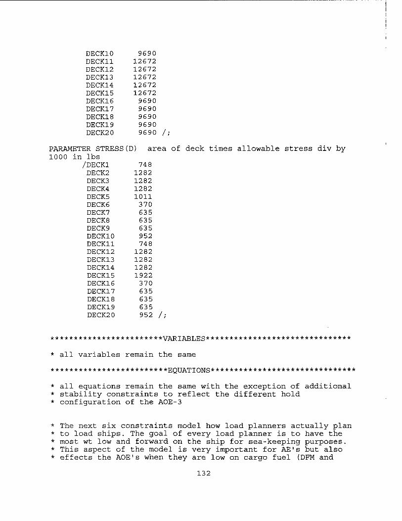
DECK10 9690 DECK11 12672 DECK12 12672 DECK13 12672 DECK14 12672 DECK15 12672 DECK16 9690 DECK17 9690 DECK18 9690 DECK19 9690 DECK2 0 9690
PARAMETER STRESS(D) ar 1000 in lbs
/DECK1 748 DECK2 1282 DECK3 1282 DECK4 1282 DECK5 1011 DECK6 370 DECK7 635 DECK8 635 DECK9 635 DECK10 952 DECK11 748 DECK12 1282 DECK13 1282 DECK14 1282 DECK15 1922 DECK16 370 DECK17 635 DECK18 635 DECK19 635 DECK2 0 952
/;
;a of deck times allowable stress div by
/;
*********************** *VARIABLES *******************************
* all variables remain the same
************************* EQUATIONS *******************************
* all equations remain the same with the exception of additional * stability constraints to reflect the different hold * configuration of the AOE-3
* The next six constraints model how load planners actually plan * to load ships. The goal of every load planner is to have the * most wt low and forward on the ship for sea-keeping purposes. * This aspect of the model is very important for AE's but also * effects the AOE's when they are low on cargo fuel (DFM and
132
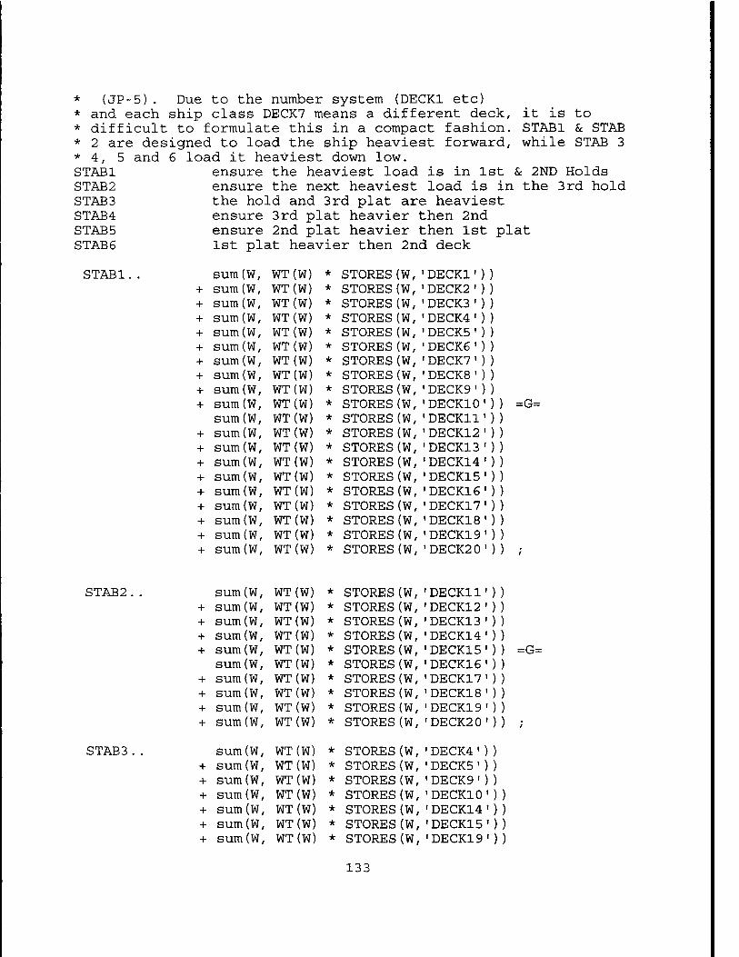
* (JP-5) . * and each * difficult * 2 are des * 4, 5 and STAB1 STAB2 STAB 3 STAB4 STAB5 STAB 6
Due to the number system (DECK1 etc) ship class DECK7 means a different deck, it is to to formulate this in a compact fashion. STAB1 & STAB igned to load the ship heaviest forward, while STAB 3 6 load it heaviest down low.
ensure the heaviest load is in 1st & 2ND Holds ensure the next heaviest load is in the 3rd hold the hold and 3rd plat are heaviest ensure 3rd plat heavier then 2nd ensure 2nd plat heavier then 1st plat 1st plat heavier then 2nd deck
STAB1
STAB2
STAB 3
sum(W, WT(W) * STORES(W,' DECK1')) + sum(W, WT(W) * STORES(W,' DECK2')) + sum(W, WT(W) * STORES(W,' DECK3')) + sum(W, WT(W) * STORES(W,* DECK4')) + sum(W, WT(W) * STORES(W,' DECK5')) + sum(W, WT(W) * STORES(W,' DECK6')) + sum(W, WT(W) * STORES(W,' DECK7')) + sum(W, WT(W) * STORES(W,' DECK8')) + sum(W, WT(W) * STORES(W,' DECK9')) + sum (W, WT(W) * STORES(W,' DECK10'))
sum (W, WT(W) * STORES(W,' DECK11')) + sum(W, WT(W) * STORES(W,' DECK12')) + sum (W, WT(W) * STORES(W, DECK13■)) + sum(W, WT(W) * STORES(W, DECK14')) + sum(W, WT(W) * STORES(W, DECK15')) + sum(W WT(W) * STORES(W, DECK16')) + sum(W WT(W) * STORES(W, DECK17')) + sum(W WT(W) * STORES(W, DECK18')) + sum(W WT(W) * STORES(W, DECK19')) + sum (W WT(W) * STORES(W, DECK201))
sum (W WT(W) * STORES(W, DECK11')) + sum(W , WT(W) * STORES(W, DECK12')) + sum(W , WT(W) * STORES(W, DECK13■)) + sum(W , WT(W) * STORES(W, DECK14')) + sum (W , WT(W) * STORES(W, DECK15'))
sum (W , WT(W) * STORES(W, DECK16')) + sum(W , WT(W) * STORES(W, 'DECK17')) + sum (W , WT(W) * STORES(W, 'DECK18')) + sum (W , WT(W) * STORES(W, ■DECK19')) + sum(W , WT(W) * STORES(W, ■DECK20*))
sum(W , WT(W) * STORES(W, ■DECK4')) + sum(W , WT(W) * STORES(W, 1DECK5')) + sum (W , WT(W) * STORES(W, ■DECK9')) + sum(W , WT(W) * STORES(W, ■DECK10*)) + sum(W , WT(W) * STORES(W, 'DECK14')) + sum(W , WT(W) * STORES(W, 'DECK15')) + sum (W , WT(W) * STORES(W, ■DECK19'))
=G=
=G=
133
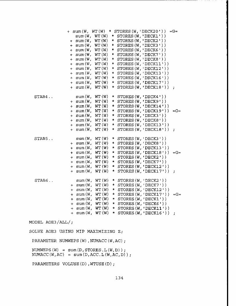
+ sum(W, WT(W)
STAB4
STAB5.
STAB6..
sum sum sum sum sum sum sum sum sum sum sum sum
sum sum sum sum sum sum sum sum
sum sum sum sum sum sum sum sum
sum sum sum sum sum sum sum sum
MODEL A0E3/ALL/;
(W, WT(W) (W, WT(W) (W, WT(W) (w, WT(W) (W, WT(W) (W, WT(W) (w, WT(W) (w, WT(W) (w, WT(W) (W, WT(W) (w, WT(W) (W, WT(W)
(w, WT(W) (W WT(W) (w WT(W) (w WT(W) (W WT(W) (W WT(W) (W WT(W) (w WT(W)
(W WT(W) (W WT(W) (W WT(W) (W WT(W) (W , WT(W) (w , WT(W) (W , WT(W) (W , WT(W)
(W , WT(W) (W , WT (W) (W , WT(W) (w , WT(W) (W , WT(W) (W , WT(W) (w , WT(W) (W , WT(W)
* STORES(W, * STORES(W * STORES(W * STORES(W * STORES(W * STORES(W * STORES(W * STORES(W * STORES(W * STORES(W * STORES(W * STORES(W * STORES(W
STORES(W STORES(W STORES(W STORES(W STORES(W STORES(W. STORES(W. STORES(W.
STORES(W STORES(W STORES(W STORES(W STORES(W STORES(W STORES(W STORES(W
STORES(W STORES(W STORES(W STORES(W STORES(W STORES(W STORES(W STORES(W
SOLVE A0E3 USING MIP MAXIMIZING Z;
PARAMETER NUMWEPS(W),NUMACC(W,AC);
NUMWEPS(W) = sum(D,STORES.L(W,D)); NUMACC(W,AC) = sum(D,ACC.L(W/AC,D));
PARAMETERS VOLUSE(D),WTUSE(D);
DECK20' DECK1■ DECK2■ DECK3■ DECK6' DECK7' DECK8' DECK11 DECK12 DECK13 DECK16 DECK17 DECK18
DECK4' DECK9' DECK14 DECK19 DECK3 * DECK8' DECK13 DECK18
DECK3' DECK8 * DECK13 DECK18 DECK2' DECK7' DECK12 DECK17
DECK2■ DECK7' DECK12 DECK17 DECK1' DECK6' DECK11 DECK16'
=G=
=G=
=G=
=G=
134
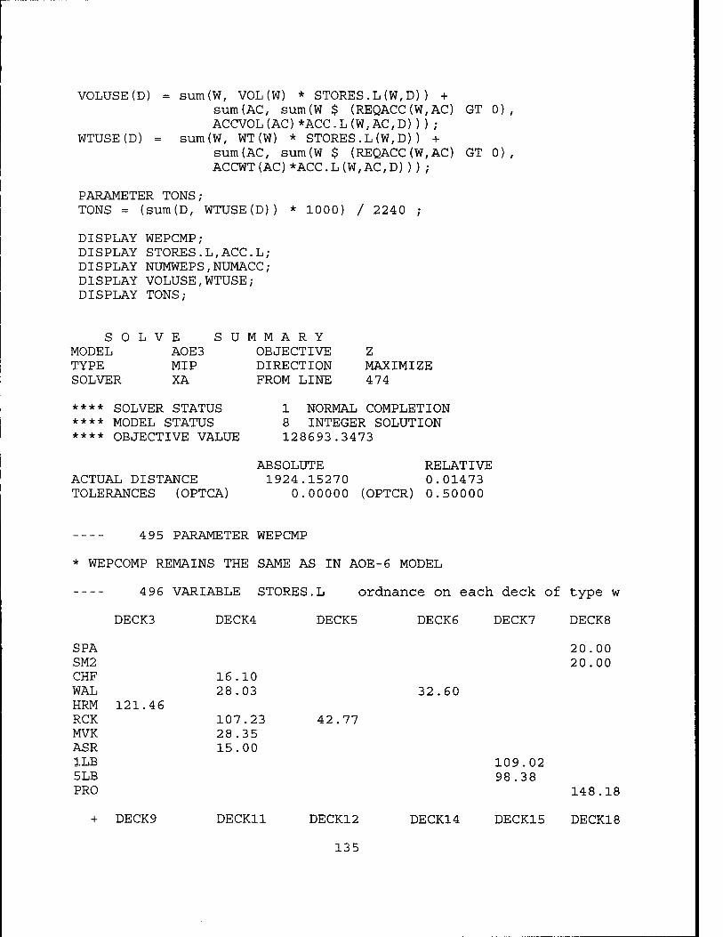
VOLUSE(D) = sum(W, VOL(W) * STORES.L(W,D)) + sum(AC, sum(W $ (REQACC(W,AC) GT 0), ACCVOL(AC)*ACC.L(W,AC,D)));
WTUSE(D) = sura(W, WT(W) * STORES.L(W,D)) + sum(AC, sum(W $ (REQACC(W,AC) GT 0), ACCWT(AC)*ACC.L(W,AC,D)));
PARAMETER TONS; TONS = (sutn(D, WTUSE(D)) * 1000) / 2240 ;
DISPLAY WEPCMP; DISPLAY STORES.L,ACC.L; DISPLAY NUMWEPS,NUMACC; DISPLAY VOLUSE,WTUSE; DISPLAY TONS;
SOLVE SUMMARY MODEL AOE3 OBJECTIVE TYPE MIP DIRECTION SOLVER XA FROM LINE
MAXIMIZE 474
**** SOLVER STATUS **** MODEL STATUS **** OBJECTIVE VALUE
ACTUAL DISTANCE TOLERANCES (OPTCA)
1 NORMAL COMPLETION 8 INTEGER SOLUTION 128693.3473
ABSOLUTE RELATIVE 1924.15270 0.01473
0.00000 (OPTCR) 0.50000
4 95 PARAMETER WEPCMP
* WEPCOMP REMAINS THE SAME AS IN AOE-6 MODEL
496 VARIABLE STORES.L ordnance on each deck of type w
DECK3 DECK4 DECK5 DECK6 DECK7
SPA SM2 CHF 16.10 WAL 28.03 HRM 121.46 RCK 107.23 42.77 MVK 28.35 ASR 15.00 1LB 5 LB PRO
+ DECK 9 DECK11 DECK12
135
32.60
DECK14
109.02 98.38
DECK15
DECK8
20.00 20.00
148.18
DECK18
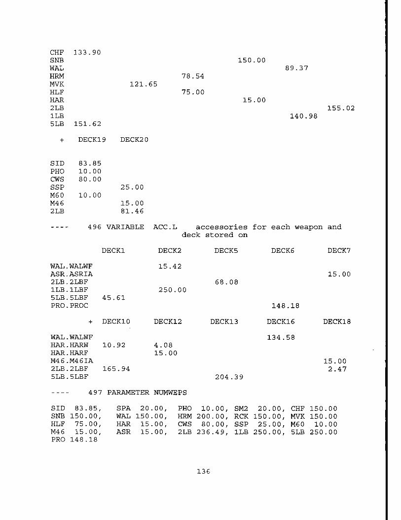
CHF 133.90 SNB 150.00 WAL HRM 78.54 MVK 121.65 HLF 75.00 HAR 15.00 2 LB 1LB 5 LB 151.62
+ DECK19 DECK2 0
SID 83.85 PHO 10.00 CWS 80.00 SSP 25.00 M60 10.00 M46 15.00 2 LB 81.46
89.37
155.02 140.98
496 VARIABLE ACC.L accessories for each weapon and deck stored on
DECK1 DECK6 DECK7
WAL.WALWF 15.42 ASR.ASRIA 2LB.2LBF 68.08 1LB.1LBF 250.00 5LB.5LBF 45.61 PRO.PROC
+ DECK10 DECK12 DECK13
WAL.WALWF HAR.HARW 10.92 4.08 HAR.HARF 15.00 M46.M46IA 2LB.2LBF 165.94 5LB.5LBF 204.39
15.00
148.18
DECK16
134.58
DECK18
15.00 2.47
497 PARAMETER NUMWEPS
SID 83.85, SNB 150.00, HLF 75.00, M46 15.00, PRO 148.18
SPA 20.00, WAL 150.00, HAR 15.00, ASR 15.00,
PHO 10.00, HRM 200.00, CWS 80.00,
SM2 20.00, RCK 150.00, SSP 25.00,
CHF 150.00 MVK 150.00 M60 10.00
2LB 236.49, 1LB 250.00, 5LB 250.00
136
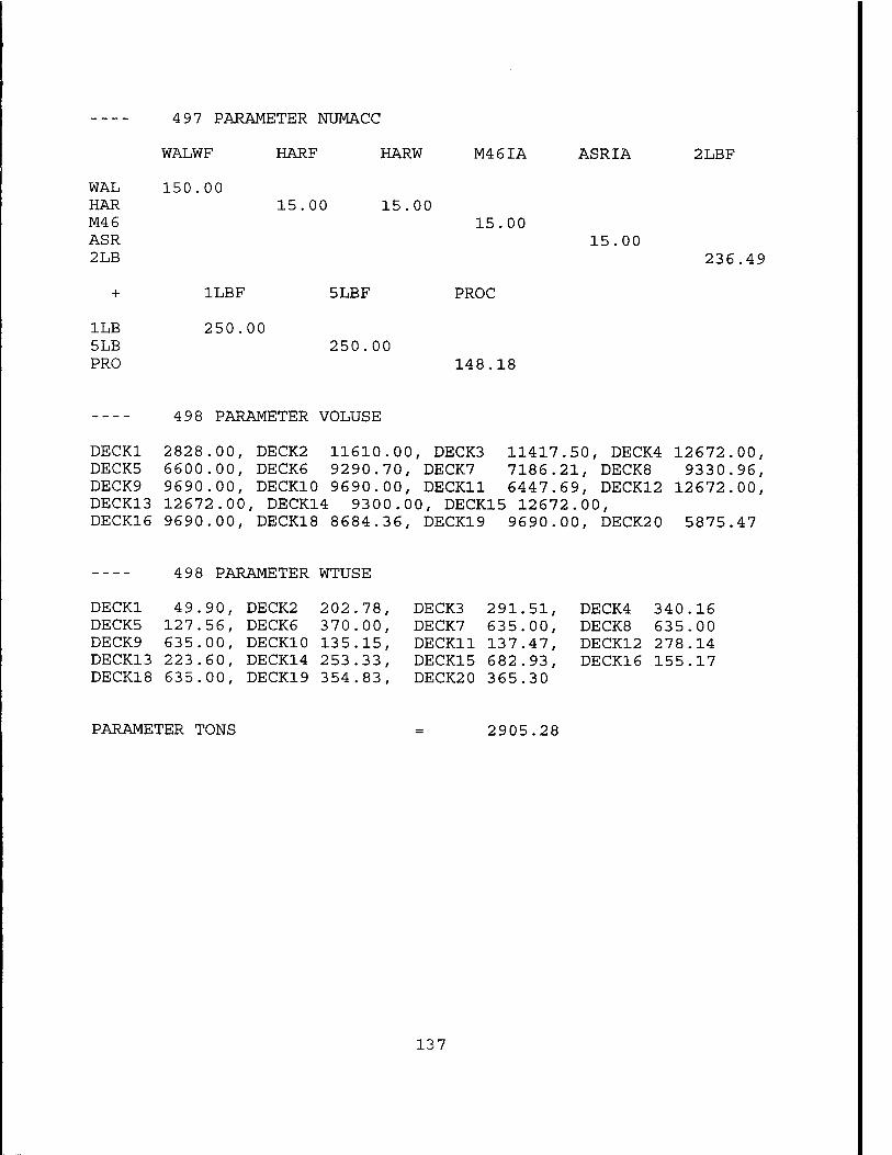
4 97 PARAMETER NUMACC
WALWF HARF HARW M4 6IA ASRIA 2LBF
WAL 150 .00 HAR 15.00 15.00 M46 15.0 ASR 2LB
+ 1LBF 5LBF PROC
1LB 250.00 5LB 250.00 PRO 148.18
15.00 236.49
498 PARAMETER VOLUSE
DECK1 2828.00, DECK2 11610.00, DECK3 11417.50, DECK4 12672.00, DECK5 6600.00, DECK6 9290.70, DECK7 7186.21, DECK8 9330.96, DECK9 9690.00, DECK10 9690.00, DECK11 6447.69, DECK12 12672.00, DECK13 12672.00, DECK14 9300.00, DECK15 12672.00, DECK16 9690.00, DECK18 8684.36, DECK19 9690.00, DECK20 5875.47
4 98 PARAMETER WTUSE
DECK1 49 90, DECK2 202 78 DECK5 127 56, DECK6 370 00 DECK9 635 00, DECK10 135 15 DECK13 223 60, DECK14 253 33 DECK18 635.00, DECK19 354.83,
DECK3 291.51, DECK7 635.00, DECK11 137.47, DECK15 682.93, DECK20 365.30
DECK4 34 0.16 DECK8 635.00 DECK12 278.14 DECK16 155.17
PARAMETER TONS 2905.28
137
138
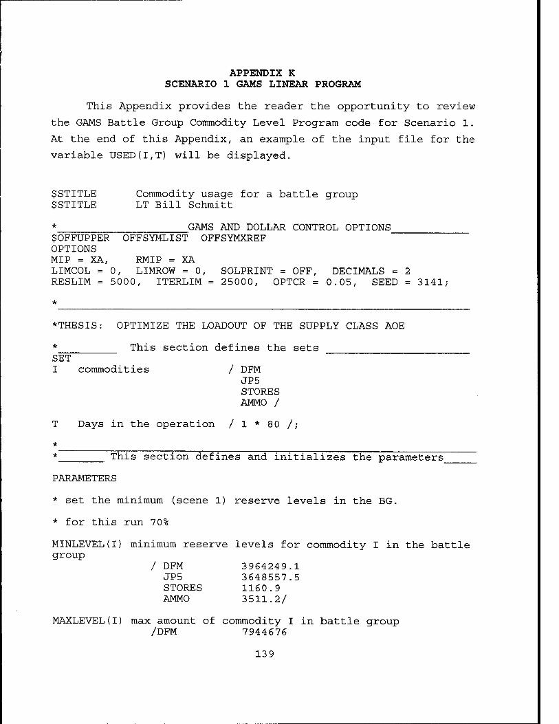
APPENDIX K SCENARIO 1 GAMS LINEAR PROGRAM
This Appendix provides the reader the opportunity to review
the GAMS Battle Group Commodity Level Program code for Scenario 1.
At the end of this Appendix, an example of the input file for the
variable USED(I,T) will be displayed.
$STITLE Commodity usage for a battle group $STITLE LT Bill Schmitt
* GAMS AND DOLLAR CONTROL OPTIONS $OFFUPPER OFFSYMLIST OFFSYMXREF OPTIONS MIP = XA, RMIP = XA LIMCOL = 0, LIMROW = 0, SOLPRINT = OFF, DECIMALS = 2 RESLIM = 5000, ITERLIM = 25000, OPTCR = 0.05, SEED = 3141;
*THESIS: OPTIMIZE THE LOADOUT OF THE SUPPLY CLASS AOE
* This section defines the sets SET I commodities / DFM
JP5 STORES AMMO /
T Days in the operation / 1 * 80 /;
This section defines and initializes the parameters
PARAMETERS
* set the minimum (scene 1) reserve levels in the BG.
* for this run 70%
MINLEVEL(I) minimum reserve levels for commodity I in the battle group
/ DFM 3964249.1 JP5 3648557.5 STORES 1160.9 AMMO 3511.2/
MAXLEVEL(I) max amount of commodity I in battle group /DFM 7944676
139
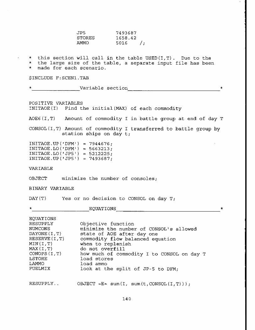
JP5 7493687 STORES 1658.42 AMMO 5016 /;
* this section will call in the table USED(I,T). Due to the * the large size of the table, a separate input file has been * made for each scenario.
$INCLUDE FrSCENl.TAB
* Variable section
POSITIVE VARIABLES INITAOE(I) Find the initial(MAX) of each commodity
AOE6(I,T) Amount of commodity I in battle group at end of day T
CONSOL(I,T) Amount of commodity I transferred to battle group by station ships on day t;
INITAOE.UP('DFM') = 7944676 INITAOE.LO('DFM') = 5663213 INITAOE.LO('JP5') = 5212225 INITAOE.UP('JP5') = 7493687
VARIABLE
OBJECT minimize the number of consoles;
BINARY VARIABLE
DAY(T) Yes or no decision to CONSOL on day T;
* EQUATIONS
EQUATIONS RESUPPLY NUMCONS DAYONE(I,T) RESERVE(I,T) MIN(I,T) MAX(I,T) CONOPS(I,T) LSTORE LAMMO FUELMIX
Objective function minimize the number of CONSOL's allowed state of AOE after day one commodity flow balanced equation when to replenish do not overfill how much of commodity I to CONSOL on day T load stores load ammo look at the split of JP-5 to DFM;
RESUPPLY. OBJECT =E= sum(I, sum(t,CONSOL(I,T)));
140
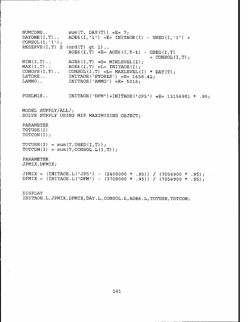
NUMCONS.. sum(T, DAY(T)) =E= 7; DAYONE(I,T) . . AOESd,1!') =E= INITAOE(I) - USED(I,'l') + CONSOL(i,'1'); RESERVE(I,T) $ (ord(T) gt 1)..
AOE6(I;T) =E= AOE6(I,T-l) -USED(I,T) + CONSOL(I,T);
MIN(I,T).. AOE6(I,T) =G= MINLEVEL(I); MAX(I,T).. AOE6(I,T) =L= INITAOE(I); CONOPS(I,T).. CONSOL(I,T) =L= MAXLEVEL(I) *DAY(T); LSTORE.. INITAOE('STORES') =E= 1658.42; LAMMO.. INITAOE('AMMO') =E= 5016;
FUELMIX.. INITAOE('DFM')+INITAOE(*JP5') =E= 13156901 * .95;
MODEL SUPPLY/ALL/; SOLVE SUPPLY USING MIP MAXIMIZING OBJECT;
PARAMETER TOTUSE(I) TOTCON(I);
TOTUSE(I) = sum(T,USED(I,T)); TOTCON(I) = sum(T,CONSOL.L(I,T));
PARAMETER JPMIX,DFMIX;
JPMIX = (INITAOE.L('JP5') - (2400000 * .95)) / (7056900 * .95); DFMIX = (INITAOE.L(■DFM') - (3700000 * .95)) / (7056900 * .95);
DISPLAY INITAOE.L,JPMIX,DFMIX,DAY.L,CONSOL.L,AOE6.L,TOTUSE,TOTCON;
141
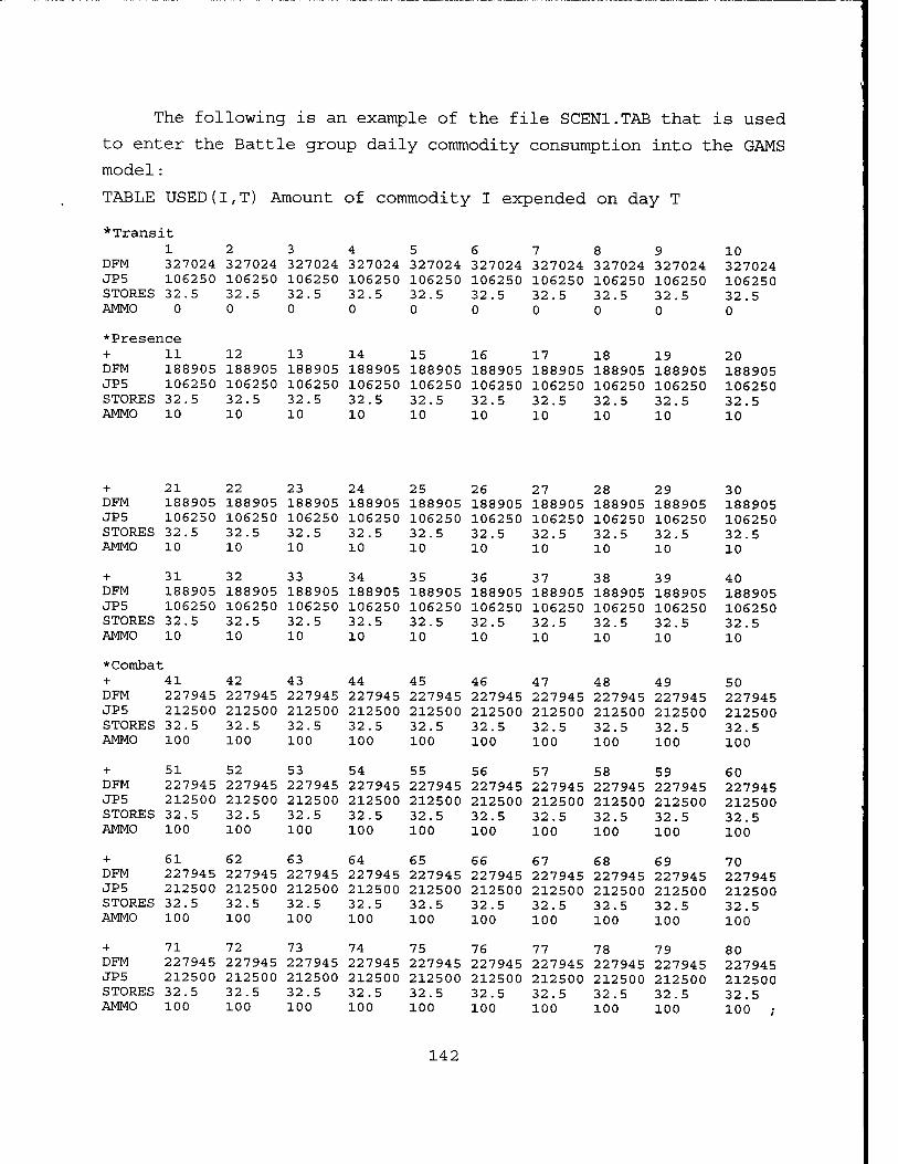
The following is an example of the fi .le SCEN1.TAE that
1
is used
to enter the Battle group daily commodity consumption into the GAMS model :
TABLE USED(I,T) Amount of commodity I expended on day T
*Trans it 1 2 3 4 5 6 7 8 9 10
DFM 327024 327024 327024 327024 327024 327024 327024 327024 327024 327024 JP5 106250 106250 106250 106250 106250 106250 106250 106250 106250 106250 STORES 32.5 32.5 32.5 32.5 32.5 32.5 32.5 32.5 32.5 32.5 AMMO 0 0 0 0 0 0 0 0 0 0
♦Presence + 11 12 13 14 15 16 17 18 19 20 DFM 188905 188905 188905 188905 188905 188905 188905 188905 188905 188905 JP5 106250 106250 106250 106250 106250 106250 106250 106250 106250 106250 STORES 32.5 32.5 32.5 32.5 32.5 32.5 32.5 32.5 32.5 32.5 AMMO 10 10 10 10 10 10 10 10 10 10
+ 21 22 23 24 25 26 27 28 29 30 DFM 188905 188905 188905 188905 188905 188905 188905 188905 188905 188905 JP5 106250 106250 106250 106250 106250 106250 106250 106250 106250 106250 STORES 32.5 32.5 32.5 32.5 32.5 32.5 32.5 32.5 32.5 32.5 AMMO 10 10 10 10 10 10 10 10 10 10
+ 31 32 33 34 35 36 37 38 39 40 DFM 188905 188905 188905 188905 188905 188905 188905 188905 188905 188905 JP5 106250 106250 106250 106250 106250 106250 106250 106250 106250 106250 STORES 32.5 32.5 32.5 32.5 32.5 32.5 32.5 32.5 32.5 32.5 AMMO 10 10 10 10 10 10 10 10 10 10
*Combat + 41 42 43 44 45 46 47 48 49 50 DFM 227945 227945 227945 227945 227945 227945 227945 227945 227945 227945 JP5 212500 212500 212500 212500 212500 212500 212500 212500 212500 212500 STORES 32.5 32.5 32.5 32.5 32.5 32.5 32.5 32.5 32.5 32.5 AMMO 100 100 100 100 100 100 100 100 100 100
+ 51 52 53 54 55 56 57 58 59 60 DFM 227945 227945 227945 227945 227945 227945 227945 227945 227945 227945 JP5 212500 212500 212500 212500 212500 212500 212500 212500 212500 212500 STORES 32.5 32.5 32.5 32.5 32.5 32.5 32.5 32.5 32.5 32.5 AMMO 100 100 100 100 100 100 100 100 100 100
+ 61 62 63 64 65 66 67 68 69 70 DFM 227945 227945 227945 227945 227945 227945 227945 227945 227945 227945 JP5 212500 212500 212500 212500 212500 212500 212500 212500 212500 212500 STORES 32.5 32.5 32.5 32.5 32.5 32.5 32.5 32.5 32.5 32.5 AMMO 100 100 100 100 100 100 100 100 100 100
+ 71 72 73 74 75 76 77 78 79 80 DFM 227945 227945 227945 227945 227945 227945 227945 227945 227945 227945 JP5 212500 212500 212500 212500 212500 212500 212500 212500 212500 212500 STORES 32.5 32.5 32.5 32.5 32.5 32.5 32.5 32.5 32.5 32.5 AMMO 100 100 100 100 100
142
100 100 100 100 100 ;
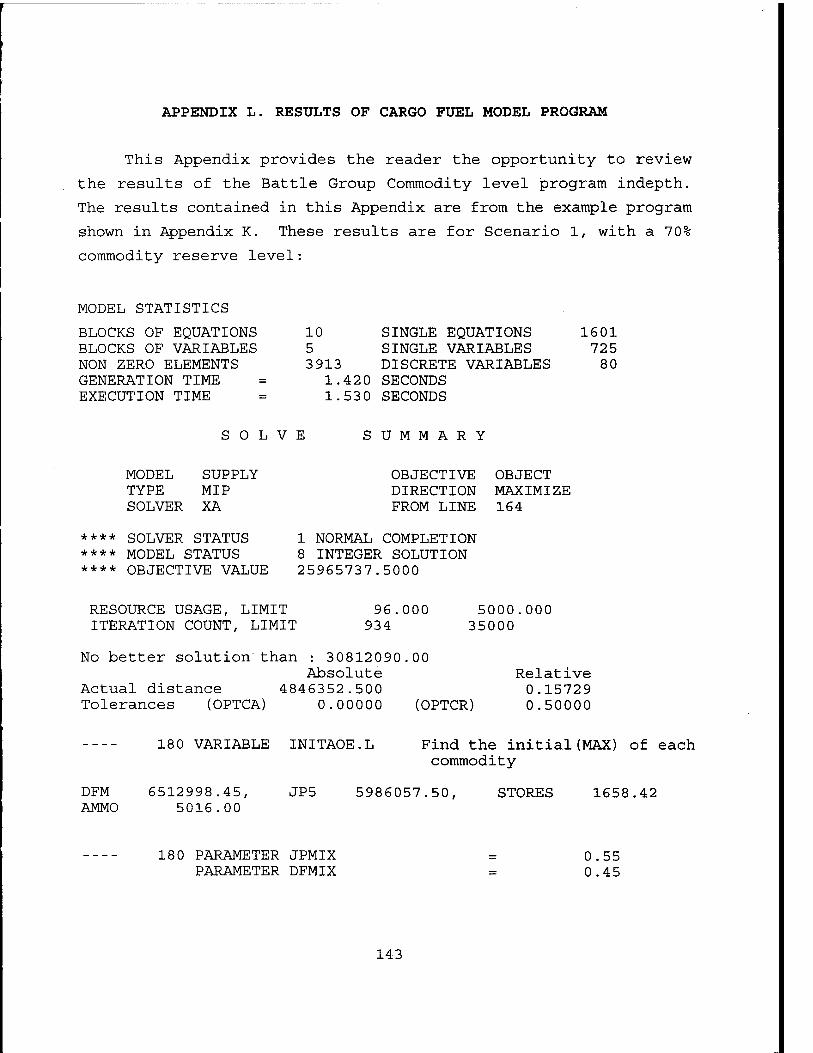
APPENDIX L. RESULTS OF CARGO FUEL MODEL PROGRAM
This Appendix provides the reader the opportunity to review
the results of the Battle Group Commodity level program indepth.
The results contained in this Appendix are from the example program
shown in Appendix K. These results are for Scenario 1, with a 70%
commodity reserve level:
MODEL STATISTICS
BLOCKS OF EQUATIONS BLOCKS OF VARIABLES NON ZERO ELEMENTS GENERATION TIME EXECUTION TIME
10 SINGLE EQUATIONS 1601 5 SINGLE VARIABLES 725 3 913 DISCRETE VARIABLES 80
1.420 SECONDS 1.53 0 SECONDS
SOLVE SUMMARY
MODEL SUPPLY TYPE MIP SOLVER XA
OBJECTIVE OBJECT DIRECTION MAXIMIZE FROM LINE 164
**** SOLVER STATUS **** MODEL STATUS **** OBJECTIVE VALUE
1 NORMAL COMPLETION 8 INTEGER SOLUTION 25965737.5000
RESOURCE USAGE, LIMIT ITERATION COUNT, LIMIT
96.000 934
5000.000 35000
No better solution than : 30812090.00 Absolute Relative
Actual distance 4846352.500 0.15729 Tolerances (OPTCA) 0.00000 (OPTCR) 0.50000
180 VARIABLE INITAOE.L
DFM 6512998.45, AMMO 5016.00
Find the initial(MAX) of each commodity
JP5 5986057.50, STORES 1658.42
180 PARAMETER JPMIX PARAMETER DFMIX
0.55 0.45
143
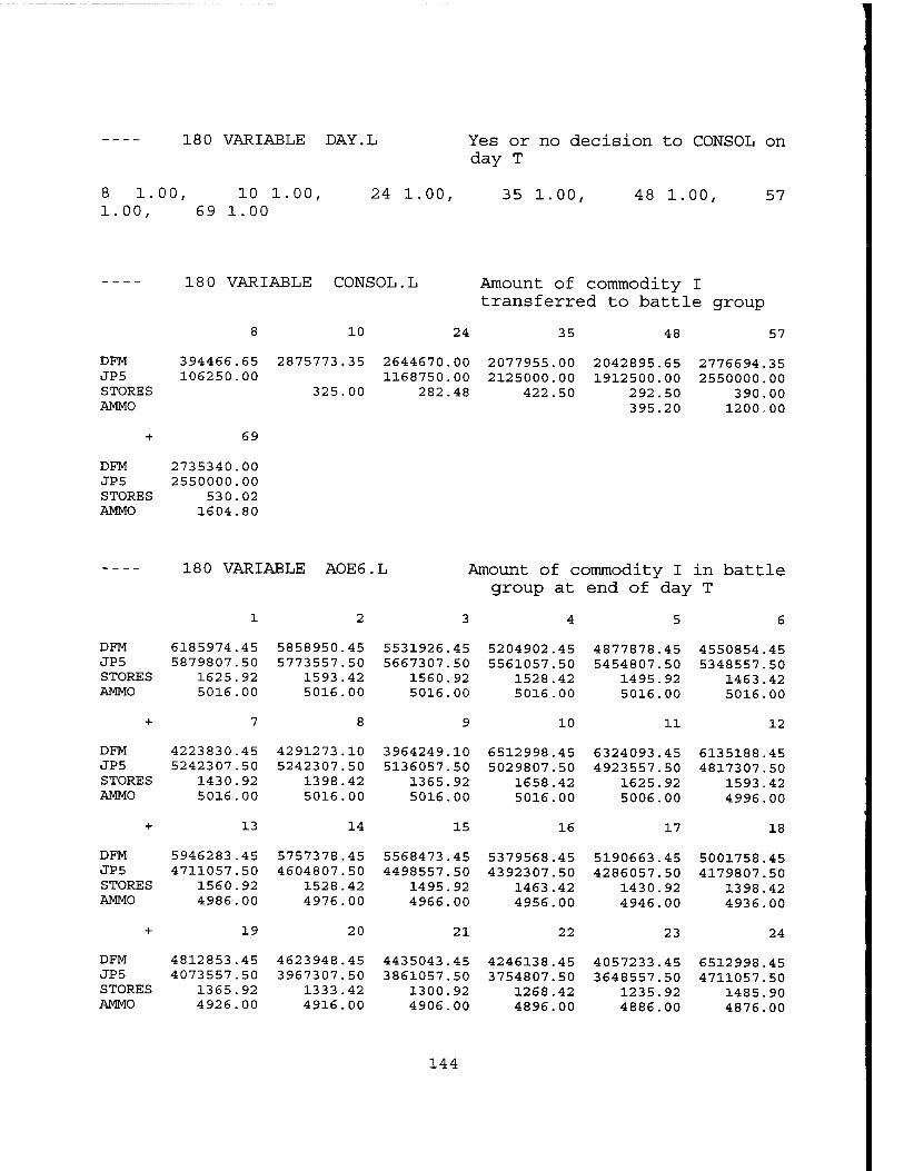
180 VARIABLE DAY.L Yes or no decision to CONSOL on day T
8 1.00, 10 1.00, 24 1.00, 35 1.00, 48 1.00, 57 1.00, 69 1.00
180 VARIABLE CONSOL.L
10
Amount of commodity I transferred to battle group
24 35 48 57
DFM 394466.65 2875773.35 2644670 00 2077955 00 2042895 65 2776694 35 JP5 106250.00 1168750 00 2125000 00 1912500 00 2550000 00 STORES 325.00 282 48 422 50 292 50 390 00 AMMO 395 20 1200 00
+ 69
DFM 2735340.00 JP5 2550000.00 STORES 53 0.02 AMMO 1604.80
180 VARIABLE AOE6.L Amount of commodity I in battle group at end of day T
DFM 6185974 45 5858950 45 5531926 45 5204902 45 4877878 45 4550854 45 JP5 5879807 50 5773557 50 5667307 50 5561057 50 5454807 50 5348557 50 STORES 1625 92 1593 42 1560 92 1528 42 1495 92 1463 42 AMMO 5016 00 5016 00 5016 00 5016 00 5016 00 5016 00
10 11 12
DFM 4223830 45 4291273 10 3964249 10 6512998 45 6324093 45 6135188 45 JP5 5242307 50 5242307 50 5136057 50 5029807 50 4923557 50 4817307 50 STORES 1430 92 1398 42 1365 92 1658 42 1625 92 1593 42 AMMO 5016 00 5016 00 5016 00 5016 00 5006 00 4996 00
13 14 15 16 17 18
DFM 5946283 45 5757378 45 5568473 45 5379568 45 5190663 45 5001758 45 JP5 4711057 50 4604807 50 4498557 50 4392307 50 4286057 50 4179807 .50 STORES 1560 92 1528 42 1495 92 1463 42 1430 92 1398 42 AMMO 4986 00 4976 00 4966 00 4956 00 4946 00 4936 00
19 20 21 22 23 24
DFM 4812853 45 4623948 45 4435043 45 4246138 45 4057233 45 6512998 45 JP5 4073557 50 3967307 50 3861057 50 3754807 50 3648557 50 4711057 50 STORES 1365 92 1333 42 1300 92 1268 42 1235 92 1485 90 AMMO 4926 00 4916 00 4906 00 4896 00 4886 00 4876 00
144
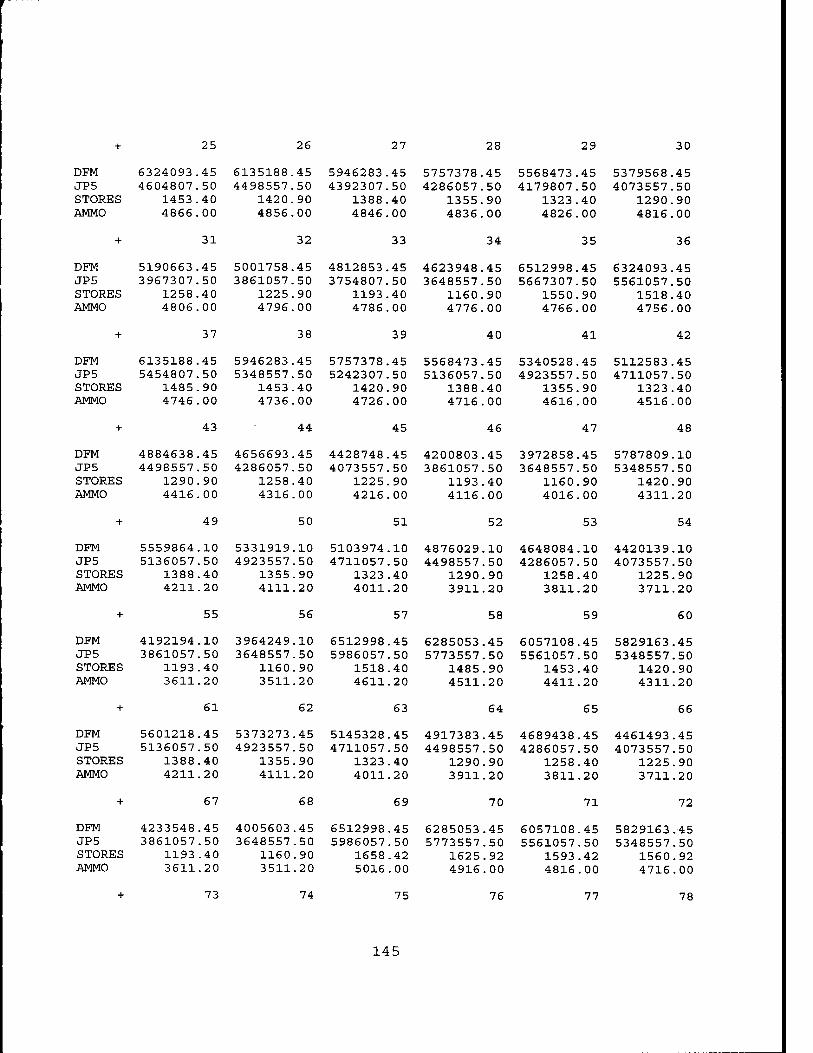
25 26 27 28 29 30
DFM 6324093.45 JP5 4604807.50 STORES 1453.40 AMMO 4866.00
6135188.45 4498557.50
1420.90 4856.00
5946283.45 4392307.50
1388.40 4846.00
5757378.45 4286057.50
1355.90 4836.00
5568473.45 4179807.50
1323.40 4826.00
5379568.45 4073557.50
1290.90 4816.00
31 32 33 34 35 36
DFM 5190663 45 5001758 45 4812853 45 4623948 45 6512998 45 6324093 45 JP5 3967307 50 3861057 50 3754807 50 3648557 50 5667307 50 5561057 50 STORES 1258 40 1225 90 1193 40 1160 90 1550 90 1518 40 AMMO 4806 00 4796 00 4786 00 4776 00 4766 00 4756 00
37 38 39 40 41 42
DFM 6135188 45 5946283 45 5757378 45 5568473 45 5340528 45 5112583 45 JP5 5454807 50 5348557 50 5242307 50 5136057 50 4923557 50 4711057 50 STORES 1485 90 1453 40 1420 90 1388 40 1355 90 1323 .40 AMMO 4746 00 4736 .00 4726 00 4716 00 4616 00 4516 .00
43 44 45 46 47 48
DFM 4884638.45 JP5 4498557.50 STORES 1290.90 AMMO 4416.00
4656693.45 4286057.50
1258.40 4316.00
4428748.45 4073557.50
1225.90 4216.00
4200803.45 3861057.50
1193.40 4116.00
3972858.45 3648557.50
1160.90 4016.00
5787809.10 5348557.50
1420.90 4311.20
49 50 51 52 53 54
DFM 5559864 10 5331919 10 5103974 10 4876029 10 4648084 10 4420139 10 JP5 5136057 50 4923557 50 4711057 50 4498557 50 4286057 50 4073557 50 STORES 1388 40 1355 90 1323 40 1290 90 1258 40 1225 90 AMMO 4211 20 4111 20 4011 20 3911 20 3811 20 3711 20
55 56 57 58 59 60
DFM 4192194 10 3964249 10 6512998 45 6285053 45 6057108 45 5829163 45 JP5 3861057 50 3648557 50 5986057 50 5773557 50 5561057 50 5348557 50 STORES 1193 40 1160 90 1518 40 1485 90 1453 40 1420 90 AMMO 3611 20 3511 20 4611 20 4511 20 4411 20 4311 20
61 62 63 64 65 66
DFM 5601218 45 5373273 45 5145328 45 4917383 45 4689438 45 4461493 45 JP5 5136057 50 4923557 50 4711057 50 4498557 50 4286057 50 4073557 50 STORES 1388 40 1355 90 1323 40 1290 90 1258 40 1225 90 AMMO 4211 20 4111 20 4011 20 3911 20 3811 20 3711 20
67 68 69 70 71 72
DFM 4233548 45 4005603 45 6512998 45 6285053 45 6057108 45 5829163 45 JP5 3861057 50 3648557 50 5986057 50 5773557 50 5561057 50 5348557 50 STORES 1193 40 1160 90 1658 42 1625 92 1593 42 1560 92 AMMO 3611 20 3511 20 5016 00 4916 00 4816 00 4716 00
73 74 75 76 77 78
145
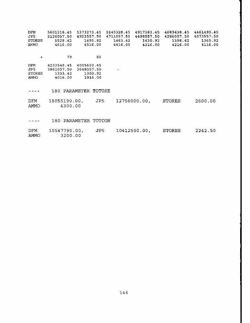
DFM 5601218 45 5373273 45 5145328 45 4917383 45 4689438 45 4461493 45 JP5 5136057 50 4923557 50 4711057 50 4498557 50 4286057 50 4073557 50 STORES 1528 42 1495 92 1463 42 1430 92 1398 42 1365 92 AMMO 4616 00 4516 00 4416 00 4316 00 4216 00 4116 00
79 80
DFM 4233548 45 4005603 45 JP5 3861057 50 3648557 50 STORES 1333 42 1300 92 AMMO 4016 00 3916 00
180 PARAMETER TOTUSE
DFM 18055190.00, AMMO 4300.00
JP5 12750000.00, STORES 2600.00
180 PARAMETER TOTCON
DFM 15547795.00, AMMO 3200.00
JP5 10412500.00, STORES 2242.50
146
LIST OF REFERENCES
1. Secretary of the Navy, ...From the Sea: Preparing the Naval Service for the 21st Century, Navy and Marine Corps White Paper, September, 1992.
2. Miller, M., J. Hammet and T. Murphy, "The Development of the U.S. Navy Underway Replenishment Fleet", paper presented at the annual meeting of the Society of Naval Architects and Marine Engineers, New York, November 1987.
3. Code of Federal Regulations, Parts 100-177, U.S. Government Printing Office, Washington DC 1993.
4. A Lower Cost UNREP System, Underway Replenishment Department, Naval Surface Warfare Center, Port Hueneme Division, January 1993.
5. Combat Logistics Force Ships Underway Replenishment Manning, Underway Replenishment Department, Naval Surface Warfare Center, Port Hueneme Division, January 1993.
6. Schrady, D., et al., Predicting Ship Fuel Consumption, Naval Postgraduate School, NPSOR-91-03, October 1990.
7. Naval Sea Systems Command, SWO-AC-SAF-010, Storage of Ordnance on Department of Navy Controlled Shipping, September 1988.
8. Reeger, Christopher M., Optimal Cargo Volume Mix For a Multi-Product Kaiser Class Oiler, M.S. Thesis, Naval Postgraduate School, Monterey, California, September 1993.
9. Rowland, John K., Optimal Load Lists of Ordnance For the AE-26 Class Ammunition Ship, M.S. Thesis, Naval Postgraduate School, Monterey, California, September 1988.
10. Brooke, A., Kendrick, D. and Meeraus, A., GAMS, A User's Guide, Release 2.25, The Scientific Press, 1992.
11. Lindsay, G.F., Constructing Interval Scales from Categorical Judgements, Unpublished Paper, Naval Postgraduate School, Monterey, California, September 1981.
12. Guadalupe, L.A., Prioritization of Advanced Based Functional Components, M.S. Thesis, Naval Postgraduate School, Monterey, California, September 1988.
13. Crawford, P.M., Dynamic Study of Factors Impacting on Combat Power, M.S. Thesis, Naval Postgraduate School, Monterey, California, March 1988.
147
14. AOE 6 Final Technical Design History, Naval Sea Systems Command, February 1987.
15. Interview between Bob Aten and Diane Hien, Load Planners, Naval Weapons Station Earle, and the author, 13 December 1994.
16. Naval Sea Systems Command, NAVSEA OP 3206 VOL 1, Ammunition Storage in Cargo Magazines, October 1989.
17. Air Launched Missile Navy Ammunition Logistics Code, Weapons Support Directorate, Pacific Missile Test Center, Point Magu, California, January 1988.
18. Telephone conversation between Mark Miller, AOE-6 Project Director, Naval Sea Systems Command, and the author, 12 December 1994.
19. Telephone conversation between Marvin Miller, Underway Replenishment Department, Naval Surface Warfare Center, Port Hueneme Division, and the author, 10 January 1995.
20. COMNAVSEASYSCOM, Washington DC, Naval Message, Subject: Ammunition Height Limitations on Ammunition and Amphibious Ships, 212030Z May 86.
21. Naval Weapons Station, Earle NJ, "Useable Cube per Level for AE 26 Class and AOE 3/4 Class", presented to author by Bob Aten, Load Planner, Naval Weapons Station, Earle, 13 December 1994.
22. Interview between CDR W. Kroshl, former Chief Engineer and Executive Officer aboard two AOEs, 18 January 1995.
23. CINCLANTFLT, Norfolk, VA, Naval Message, Subject: USS Seattle Recommended Ammo Load ISO JTG 95-2, 291435Z Aug 94.
24. LT Long, J.A., " OA - 4611 Logistics in Naval Warfare Paper Proposal ," paper presented by Dr. D. Schrady as part of class discussion on 20 January 1995.
25. AOE(V) Underway Replenishment Station Alignment Study, Naval Ship Weapon Systems Engineering Station for Naval Sea Systems Command, 2 9 June 1990.
26. Jane's Fighting Ships 1994-1995, Butler and Tanner Limited, 1994.
27. Schrady, D.A., "Unclassified Data Version, TACLOGS Tactical Logistics Support System Documentation of Database," Department of Operations Research, Naval Postgraduate School, Monterey, CA, March 1994.
148
28. Telephone conversation between LCDR Rezinski, Amphibious Group Three Air Operations Officer, and the author, 26 January 1995.
29. Mendenhall, W., Wackerly, D., Scheaffer, R., Mathematical Statistics with Applications, Fourth Edition, PWS-Kent Publishing Company, 1990.
30. Secretary of the Navy, Forward...From the Sea, Navy and Marine Corps White Paper, January, 1995.
31. Telephone conversation between Mr. Dick Lord, Stability Division, Naval Sea Systems Command, and the author, 31 May 1995.
32. Torgerson, Warren S., Theory and Methods of Scaling, John Wiley & Sons Inc, 1958.
149
150
INITIAL DISTRIBUTION LIST
1. Defense Technical Information Center 2 Cameron Station Alexandria, Virginia 22304-6145
2. Library, Code 052 2 Naval Postgraduate School Monterey, California 93943-5101
3. Defense Logistic Studies Information Exchange 1 U.S. Army Logistics Management College Fort Lee, Virginia 22134-5027
4 . Dr. David Schrady, Code OR/So 1 Department of Operations Research Naval Postgraduate School Monterey, California 93943-5000
5. CDR William Kroshl, Code OR/Kr 1 Department of Operations Research Naval Postgraduate School Monterey, California 93943-5000
6. LT William J. Schmitt 1 683 Comly Ave. Langhorne, Pennsylvania 19047
7. Deputy Chief of Naval Operations for Logistics 2 N424D, Department of the Navy Washington, DC 20350-2000
8 . Deputy Chief of Naval Operations 2 N8 63D, Department of the Navy Washington, DC 20350-2000
9. Naval Surface Warfare Center, Port Hueneme Div 1 Underway Replenishment Department Attn. Mr. Marvin Miller Port Hueneme, California 93043-5007
10. CDR William Schworer, N4 1 Military Sealift Command, Atlantic Military Ocean Terminal, Bayonne Building 42 Bayonne, New Jersey 07002
151
11. Commander , Combat Logistics Group ONE Building 221-2W, Naval Supply Center Oakland, California 94625
12. Commanding Officer 201 Hwy. 34 S Naval Weapons Station, Earie Colts Neck, New Jersey 07722-5021 Attn. Code 203
13. CINCLANTFLT 5162 Mitscher Ave Suite 250 Attn. N411 Norfolk, Virginia 23551-2487
14. Naval Sea Systems Command ATTN: Mr. Dick Lord Jefferson Davis Highway Arlington, Virginia 22242
15. CAPT William Schmidt, SC, USN. Fleet Logistics, J4 Commander, Second Fleet FPO AP NY 09501-6000
16. CAPT Michael R Kalas, SC, USN. Fleet Logistics, N4 Commander, Third Fleet FPO AP SF 96601-6001
17. Naval Sea Systems Command. ATTN: Mr. Mark Miller Jefferson Davis Highway Arlington, Virginia 22242
152
Recommended