Optimistic Parallel Simulation of TCP/IP over ATM Networks
by
Ming H Chong
B.S.(ComputerEngineering),Universityof Kansas,Lawrence,Kansas,1998
Submittedto theDepartmentof ElectricalEngineeringandComputerScienceandtheFaculty
of theGraduateSchoolof theUniversityof Kansasin partialfulfillment of therequirements
for thedegreeof Masterof Science
Professorin Charge
CommitteeMembers
DateThesisAccepted
Acknowledgments
I would like to expressmy gratitudeto Dr. Victor S.Frost,my advisorandcommitteechairman,for
his guidance,encouragement,andhelpful criticism throughoutthis research.I would like to thankDr.
DouglasNiehausandDr. David Peterfor servingonmy committee,providing invaluablefeedback.
I wouldliketo especiallythankSeanHousewhomI truly enjoyedworkingwith andwhoseenormous
effort haveprovidedtheProTEuSresultsherein.
Finally, I would also like to acknowledgeGeorgios Lazaroufor his many hoursof instructionon
TCP.
I dedicatethis thesisto my mother(Y.H. Tan),father(K.F. Chong),sister(S.L.Chong),brother(C.H.
Chong),anda specialaunt(Y.H. Chong)whowereeachinspirationalto me.
Abstract
DARPA’s Next GenerationInternetImplementationPlancalls for a capabilityof simula-tionsof multiprotocolnetworkswith millions of nodes.Traditionalsequentialsimulatorsarenolongeradequateto performthetask.Parallelsimulatorsandnew modelingframeworksarethebetterapproachto simulatelarge-scalenetworks.This thesisdemonstratesthefeasibilityof op-timistic parallelsimulationonTCP/IPoverATM networks,andcomparestheperformanceof aparallelsimulatorto ProTEuS(adistributedemulationsystemtargetedfor network simulation)in termsof speedupandscalability. Theparallelsimulatorusedin this studyis Georgia Tech.TimeWarp(GTW) whichperformsparalleldiscreteeventsimulationonshared-memorymulti-processormachine.Network modelshave beendevelopedto constructlarge-scaleTCP/IPoverATM scenariosto evaluatetheperformanceof GTW. Resultsindicatethat large-scalenetworksimulationcangreatlybenefitfrom optimisticparallelsimulatordueto GTW’scapabilityin ex-ploiting parallelism.However, GTW lacksscalability, in termsof network size,whencomparedto ProTEuS.
Contents
1 Intr oduction 1
1.1 ParallelDiscreteEventSimulation . . . . . . . . . . . . . . . . . . . . . . . . 2
1.1.1 Conservative approach. . . . . . . . . . . . . . . . . . . . . . . . . . 3
1.1.2 Optimisticapproach:TimeWarp . . . . . . . . . . . . . . . . . . . . . 4
1.2 Motivation . . . . . . . . . . . . . . . . . . . . . . . . . . . . . . . . . . . . . 5
1.3 Thesisorganization . . . . . . . . . . . . . . . . . . . . . . . . . . . . . . . . 6
2 RelatedWork 7
2.1 ProportionalTimeEmulationandSimulation(ProTEuS) . . . . . . . . . . . . 7
3 Georgia TechTime Warp (GTW) 9
3.1 Overview . . . . . . . . . . . . . . . . . . . . . . . . . . . . . . . . . . . . . 9
3.2 GTW kernel . . . . . . . . . . . . . . . . . . . . . . . . . . . . . . . . . . . . 10
3.2.1 Logical processes. . . . . . . . . . . . . . . . . . . . . . . . . . . . . 10
3.2.2 Statesandcheckpointing. . . . . . . . . . . . . . . . . . . . . . . . . 11
3.2.3 Theeventqueuedatastructure . . . . . . . . . . . . . . . . . . . . . . 11
3.2.4 Themainschedulerloop . . . . . . . . . . . . . . . . . . . . . . . . . 13
3.2.5 ComputingGVT . . . . . . . . . . . . . . . . . . . . . . . . . . . . . 13
4 Implementation of simulation modelswith GTW 15
4.1 Overview . . . . . . . . . . . . . . . . . . . . . . . . . . . . . . . . . . . . . 15
4.2 Applicationlayer . . . . . . . . . . . . . . . . . . . . . . . . . . . . . . . . . 17
4.2.1 ABR source. . . . . . . . . . . . . . . . . . . . . . . . . . . . . . . . 17
4.2.2 VBR source. . . . . . . . . . . . . . . . . . . . . . . . . . . . . . . . 17
i
4.2.3 TCPsource . . . . . . . . . . . . . . . . . . . . . . . . . . . . . . . . 18
4.3 TCPlayer . . . . . . . . . . . . . . . . . . . . . . . . . . . . . . . . . . . . . 18
4.4 ATM SegmentationandReassembly(SAR) . . . . . . . . . . . . . . . . . . . 19
4.5 ATM network layer . . . . . . . . . . . . . . . . . . . . . . . . . . . . . . . . 20
4.5.1 Overview of ABR traffic management. . . . . . . . . . . . . . . . . . 20
4.5.2 ABR end-host . . . . . . . . . . . . . . . . . . . . . . . . . . . . . . 23
4.5.2.1 ABR sourcebehavior . . . . . . . . . . . . . . . . . . . . . 23
4.5.2.2 ABR destinationbehavior . . . . . . . . . . . . . . . . . . . 23
4.5.2.3 ABR end-hostqueueingdisciplineandtraffic shaping . . . . 24
4.5.3 SwitchBehavior . . . . . . . . . . . . . . . . . . . . . . . . . . . . . 25
4.5.3.1 Switchroutingandqueueingdiscipline . . . . . . . . . . . . 25
4.5.3.2 Switchcongestioncontrol . . . . . . . . . . . . . . . . . . . 27
4.5.3.3 EPRCA . . . . . . . . . . . . . . . . . . . . . . . . . . . . 28
5 Evaluation 30
5.1 Overview . . . . . . . . . . . . . . . . . . . . . . . . . . . . . . . . . . . . . 30
5.2 Validationof GTW modelsfor ATM Simulation . . . . . . . . . . . . . . . . . 31
5.2.1 Link Utilization . . . . . . . . . . . . . . . . . . . . . . . . . . . . . . 32
5.2.2 MeanQueueingDelay . . . . . . . . . . . . . . . . . . . . . . . . . . 32
5.2.3 ABR QueueLength. . . . . . . . . . . . . . . . . . . . . . . . . . . . 33
5.2.4 ABR SourceRate. . . . . . . . . . . . . . . . . . . . . . . . . . . . . 33
5.2.5 ExecutionTime . . . . . . . . . . . . . . . . . . . . . . . . . . . . . . 34
5.3 GTW performanceon ATM network simulation . . . . . . . . . . . . . . . . . 35
5.3.1 ScenarioA: 2 cores,4 edges,40 hosts . . . . . . . . . . . . . . . . . . 35
5.3.2 ScenarioB: 4 cores,12 edges,120hosts. . . . . . . . . . . . . . . . . 40
5.4 Effectof network characteristicson GTW performance. . . . . . . . . . . . . 44
5.4.1 Effect of feedbackloop in network: RollbacksdegradeGTW perfor-
mance . . . . . . . . . . . . . . . . . . . . . . . . . . . . . . . . . . 44
5.4.2 Effectof roundtrip time (RTT) . . . . . . . . . . . . . . . . . . . . . . 47
5.4.3 Effectof Network Size . . . . . . . . . . . . . . . . . . . . . . . . . . 51
5.5 Effectof simulationparametersonGTW performance. . . . . . . . . . . . . . 54
ii

5.5.1 Eventmemoryandstatememoryallocation . . . . . . . . . . . . . . . 54
6 Conclusionsand Futur eWork 56
iii
List of Tables
4.1 List of parametersin ABR service . . . . . . . . . . . . . . . . . . . . . . . . 21
4.2 New ACR Uponarrival of BRM . . . . . . . . . . . . . . . . . . . . . . . . . 22
4.3 Exampleroutingtable. . . . . . . . . . . . . . . . . . . . . . . . . . . . . . . 26
5.1 Clippersysteminformation . . . . . . . . . . . . . . . . . . . . . . . . . . . . 30
5.2 Systemparameters . . . . . . . . . . . . . . . . . . . . . . . . . . . . . . . . 31
5.3 MeanNormalizedLink Utilization . . . . . . . . . . . . . . . . . . . . . . . . 32
5.4 MeanABR Cell QueuingDelay . . . . . . . . . . . . . . . . . . . . . . . . . 32
5.5 ExecutionTime . . . . . . . . . . . . . . . . . . . . . . . . . . . . . . . . . . 35
5.6 ScenarioA: Sourceparameters. . . . . . . . . . . . . . . . . . . . . . . . . . 35
5.7 ScenarioA: ExecutionTime . . . . . . . . . . . . . . . . . . . . . . . . . . . 37
5.8 ScenarioB: Sourceparameters. . . . . . . . . . . . . . . . . . . . . . . . . . 41
5.9 ScenarioB: ExecutionTime . . . . . . . . . . . . . . . . . . . . . . . . . . . 42
5.10 Sourcetraffic policy . . . . . . . . . . . . . . . . . . . . . . . . . . . . . . . . 47
5.11 Executiontime vs. RoundTrip Time(RTT) . . . . . . . . . . . . . . . . . . . 49
5.12 ExecutionTimevsnetwork size . . . . . . . . . . . . . . . . . . . . . . . . . 52
iv
List of Figures
4.1 Implementation:Protocollayers . . . . . . . . . . . . . . . . . . . . . . . . . 17
4.2 ABR Traffic Management. . . . . . . . . . . . . . . . . . . . . . . . . . . . . 20
4.3 Structureof RM cell . . . . . . . . . . . . . . . . . . . . . . . . . . . . . . . 22
4.4 End-hostqueueingdiscipline . . . . . . . . . . . . . . . . . . . . . . . . . . . 24
4.5 Per-ClassQueuingin theATM switch . . . . . . . . . . . . . . . . . . . . . . 26
5.1 3-switch,5-hosttopology . . . . . . . . . . . . . . . . . . . . . . . . . . . . . 31
5.2 ABR QueueLength(zoom). . . . . . . . . . . . . . . . . . . . . . . . . . . . 33
5.3 ABR SourceRate(zoom) . . . . . . . . . . . . . . . . . . . . . . . . . . . . . 34
5.4 6 Switch40 HostTopology . . . . . . . . . . . . . . . . . . . . . . . . . . . . 36
5.5 ScenarioA: Executiontimevs NumberCPU. . . . . . . . . . . . . . . . . . . 38
5.6 ScenarioA: GTW Speedup(relative to 1 processor). . . . . . . . . . . . . . . 39
5.7 16 Switch120HostTopology . . . . . . . . . . . . . . . . . . . . . . . . . . 40
5.8 ScenarioB: Executiontimevs NumberCPU . . . . . . . . . . . . . . . . . . . 43
5.9 ScenarioB: GTW speedup(relative to 1 processor) . . . . . . . . . . . . . . . 43
5.10 RollbackpercentagevsEventmemoryallocated. . . . . . . . . . . . . . . . . 45
5.11 Numberof abortedeventvsEventmemoryallocated . . . . . . . . . . . . . . 46
5.12 Numberof fossil collectionvsEventmemoryallocated . . . . . . . . . . . . . 46
5.13 ScenarioA: Executiontimevs. RTT (fixedload) . . . . . . . . . . . . . . . . 48
5.14 ScenarioA: Executiontimevs. RTT . . . . . . . . . . . . . . . . . . . . . . . 50
5.15 Executiontime vs. network size . . . . . . . . . . . . . . . . . . . . . . . . . 53
5.16 Executiontime vs. eventmemoryallocated . . . . . . . . . . . . . . . . . . . 54
v
List of Programs
4.1 Pseudocodefor sourcereactionto backwardRM cells . . . . . . . . . . . . . 22
4.2 EPRCAuponreceptionof abackwardRM cell . . . . . . . . . . . . . . . . . 28
vi
Chapter 1
Intr oduction
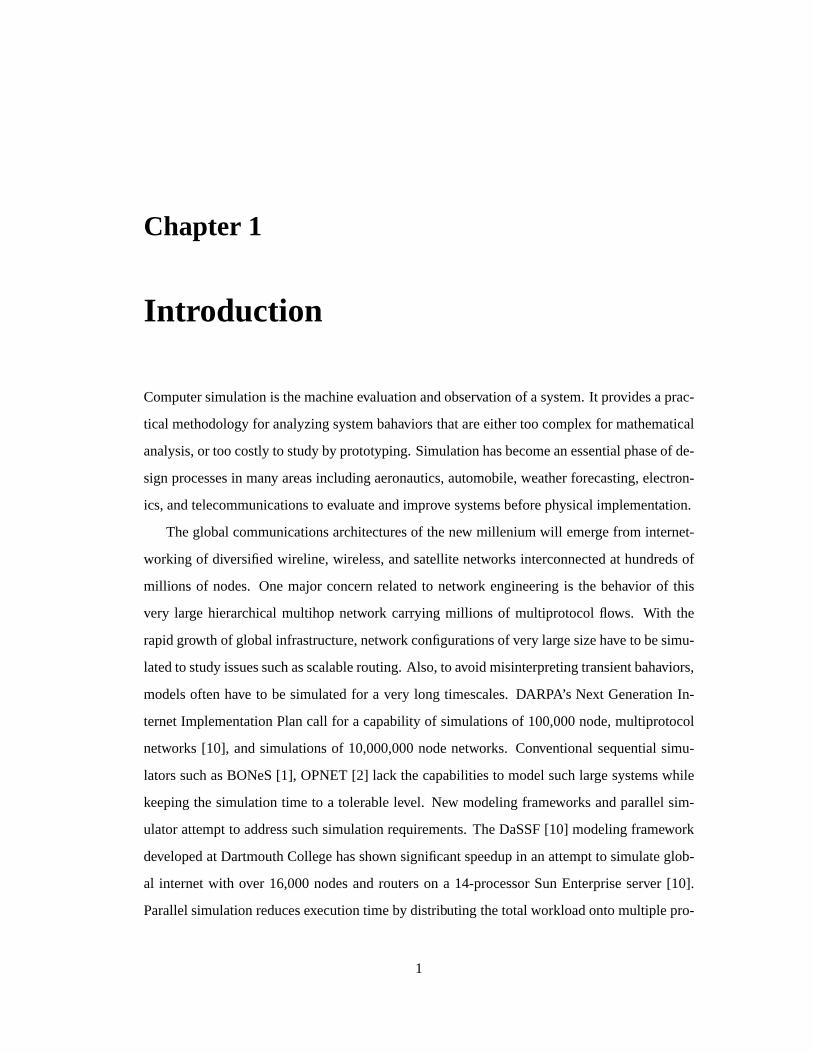
Computersimulationis themachineevaluationandobservationof asystem.It providesaprac-
tical methodologyfor analyzingsystembahaviors thatareeithertoocomplex for mathematical
analysis,or toocostlyto studyby prototyping.Simulationhasbecomeanessentialphaseof de-
signprocessesin many areasincludingaeronautics,automobile,weatherforecasting,electron-
ics,andtelecommunicationsto evaluateandimprove systemsbeforephysicalimplementation.
Theglobalcommunicationsarchitecturesof thenew millenium will emergefrom internet-
working of diversifiedwireline, wireless,andsatellitenetworks interconnectedat hundredsof
millions of nodes. Onemajor concernrelatedto network engineeringis the behavior of this
very large hierarchicalmultihop network carryingmillions of multiprotocolflows. With the
rapidgrowth of globalinfrastructure,network configurationsof very largesizehave to besimu-
latedto studyissuessuchasscalablerouting.Also, to avoid misinterpretingtransientbahaviors,
modelsoften have to be simulatedfor a very long timescales.DARPA’s Next GenerationIn-
ternetImplementationPlancall for a capabilityof simulationsof 100,000node,multiprotocol
networks [10], andsimulationsof 10,000,000nodenetworks. Conventionalsequentialsimu-
latorssuchasBONeS[1], OPNET[2] lack thecapabilitiesto modelsuchlargesystemswhile
keepingthesimulationtime to a tolerablelevel. New modelingframeworks andparallelsim-
ulatorattemptto addresssuchsimulationrequirements.TheDaSSF[10] modelingframework
developedat DartmouthCollegehasshown significantspeedupin anattemptto simulateglob-
al internetwith over 16,000nodesandrouterson a 14-processorSunEnterpriseserver [10].
Parallelsimulationreducesexecutiontimeby distributing thetotalworkloadontomultiplepro-
1
cessingentities(i.e.,processoror workstation).
However, parallel simulationhasnot not yet beenwidely usedin network researchand
industrialpracticedueto the lack of a convenientmodelingmethodologysuitablefor parallel
execution,andtheabsenceof maturesoftwareenvironment.However, parallelsimulationscan
be performedon commoditymultiprocessorservers,andon a network of workstations,all of
whicharenow commonlyavailablein academicresearchlabsandindustryfacilities.
Parallel discreteevent simulation(PDES) techniqueshave beenactively researchedand
improvedover thepastdecade.Promisingresultsof PDES’s feasibility to ATM networkssim-
ulationhave beendemonstratedby Georgia TechPADS group[4] andtheTelesimproject[31].
Experimentswith large ATM network scenarioswith 100 switchesshow that executiontime
speedupsof 3-5 are possibleon a 16-processorshared-memorySGI PowerChallenge[31].
However, therearesignificanttechnicalchallengesto overcomeregardingevent granularity,
simulationpartitioning,andloadbalancing.OtherparallelsimulatorsincludesUCLA’sParSec
[24] andPurdue’s ParaSol[23]. Most parallelsimulatorsrun on shared-memorymultiproces-
sor workstationswhereprocessorsandmemoryarecloselycoupledvia high-speedbus. The
synchronizationcanbevery fastandreliable.Nevertheless,thelow costandscalabilityof aPC
andethernet-basednetwork of workstations(NOW) makesNOW anotherattractive platform
for paralleldiscreteevent simulation. Although suchloosely-coupledsystemsrequirea more
complex inter-processorcommunicationmechanismto ensurecorrectandefficientmessagede-
livery, techniqueshavebeenproposedin Georgia TechTimeWarp(GTW) [6] andParasol[26]
to yield competingperformance.
1.1 Parallel DiscreteEvent Simulation
Discreteevent simulationis a methodusedto model real world systemsby decomposinga
systeminto a setof logical processes(LPs) autonomouslyprogressingthroughtime. All in-
terprocessorand intraprocessorcommunicationsarehandledby messagepassing(i.e., event
scheduling).Eachevent is assigneda timestamp,andmusttake placeon a destinationLP. The
resultof this event canchangethe stateof an LP, and/orgeneratenew eventsto oneor more
otherLPs.
A sequentialdiscreteevent simulationengineassignsall LPs to a single processorand
2
alwaysprocesseventsin strict logical timeorder. Sincetimeorderis strictly enforcedandonly
oneeventcanbeprocessedat a time, interprocessoreventscannever arrive atLPseitheroutof
sequenceor afteraneventwith a laterscheduledtimestamphasbeenprocessed.
Many simulationsaresufficiently large that it is impracticalto run themon a singlepro-
cessorwithin a realistic time-frame. The executiontime of a simulationexperimentcanbe
reducedby distributing theexperimentover multiple processingunits. As a matterfact,using
a multiprocessormachineis much more costeffective than building a singleprocessorwith
equivalentcomputationpower. Theoretically, large-scalesimulationwith hugenumberof LPs
inheritsmoreparallelism.Thereforethesimulationshouldbeperformedin parallelfashionon
multiprocessorcomputers.
Severalpracticalapproachesto parallelsimulationincludesreplication,conservative tech-
nique, and optimistic technique[20, 9, 13, 29]. A simple way for distributing a simulation
experimentover many processorsis to run thesamereplicationwith differentparametervalues
on separateprocessors.This replicationtechniqueis relatively efficient but it cannotextractall
theparallelismavailablein aproblem,especiallywhensearchingthroughaproblem’sparameter
space.
In practice,several processorscanbe usedin a coordinatedfashionto executethe same
simulationreplication. A simulationmodelis partitionedinto LPs. TheseLPsaredistributed
acrossmultiple processorsfor simulationandthey communicateonly by messagepassing.The
difficulty is to ensurethatall messagesandeventsin thePDESareprocessedin thesameorder
andat the samesimulationtime asin a singleprocessorsimulation. Out of orderprocessing
resultsin causalityerrors.Two popularsynchronizationtechniquesto ensureaccurateparallel
discreteeventsimulationaretheconservative andtheoptimisticapproaches.
1.1.1 Conservativeapproach
Conservative approachrepresentsan earliestwork in PDESfirst desicribedby Chandyand
Misra [9]. Simulationsynchronizedby conservative approachconsistsof a network of LPs
communicatingwith timestampedmessages.EachLP advancesits local clock andprocesses
incomingeventsonly if it coulddeterminethatnocausalityerrorswould resultfrom thisevent.
Causalityerror is detectedwhenan LP receivesa messagewith a timestampearlier thanthe
3
LP’s local clock. Deadlockis possible,dependingon theconfigurationof theLPs,whenno LP
canobtainthenecessaryinformationto advanceits clock.
Early researchhasshown that theconservative approachcannotexploit theparallelismin
many simulationmodels. The amountof parallelismis determinedby how muchthe LP can
lookaheadbasedon local knowledge. And the amountof lookaheaddependson the struture
of a simulationmodel. The conservative approachwasknown to be lesssuitablefor general
purposenetwork simulationsincethelookaheadavailableis oftentoolittle to exploit significant
parallelism.
1.1.2 Optimistic approach: Time Warp
In contrastto conservative approach,optimistic approachis ableto exploit parallelismwhen
causalityerrorsareallowedbut infrequent.It allows clock at eachLP to beadvancedwithout
regardto the statesof otherLPs. In otherwords,eachLP executeswithout waiting on other
LPsfor messages.However, a mechanismis requiredto detectandcorrectcausalityerrorsby
restoringthe simulationstatefrom a previously saved stateandresimulatingfrom that point.
Themostcommonoptimistic protocolis theTime Warpprotocol[13] originally proposedby
Jefferson[19].
TheTime Warpprotocolcorrectscausalityerrorsby saving statefor eachLP periodically,
thenrolling thesimulationbackto thepoint whencausalityerrorsaredetected.Variationsof
Time Warp have beenreported[5, 31] to performexcellenton realisticsimulationproblems.
In general,optimistic approacharemoreusefulfor generalpurposeapplicationscomparedto
conservative approachbecausethepreviousrequireslessknowledgeof a system.
A few improvementscanbedonein orderto improve TimeWarp’sperformance.An inher-
entproblemwith optimisticsimulationis theoverheadof state-saving to permit rollback. Fu-
jimoto [13] reportedthat theperformanceof anoptimisticsimulationwascut in half whenLP
statesizeincreasedfrom 100bytesto 2000bytes.Incrementalstate-saving[27] is onemethod
to reducestate-saving overheadwhereonly changesto thestatearesaved.
Rollbackoverheadis anothermajorfactorthataffectsperformance.Oneway to reducethe
costassociatedwith rollbackis to uselazy cancellation.TimeWarpusinglazy cancellationdo
not immediatelycancelthemessagespreviouslysentwhenacausalityerroris detected.Indeed,
4
themessagesarefirst comparedto thosethatwould begeneratedby thecorrectedcomputation
[13]. Only thosemessagesthatwerenotgeneratedby thecorrectedcomputationarecanceled.
Achieving load balancingmay be anotherimprovement. For parallelsimulationto work
effeciently, theLPsmustbedistributedproperlyover theavailablephysicalprocessors.Theop-
timal distribution cannotbeknown without performanceprofiling of thesimulation.Dynamic
partitioningcanbeagoodsolutionthoughit is verycomplicatedto implementin thesimulator.
During anoptimisticsimulation,processorsthatdo not have enoughLPsassignedwill be fre-
quentlyrolledbackby old messagessentfrom heavily loadedprocessorsandthusproducelittle
usefulwork. Dynamicpartitioningattemptsto assignmoreLPsto thoseprocessorswhich are
notdoingmuchusefulwork. This techniquehasbeenshown to decreaselocal time gapamong
LPs,andreducerollbackfrequency.
1.2 Moti vation
Most parallel simulationworks doneon large-scaleATM network have beenfocusingtheir
effort on two distinct areas.First, they exploit inherentparallelismof ATM network scenario
to achieve maximumpossiblespeedup.Thesecondtaskis to studyATM network performance
associatedwith variousqueuingdisciplinesanddifferent traffic flows generatedfrom video,
audio,anddatasources.However, theissueof how parallelsimulatorreactsto certainnetwork,
particularlytheTCPoverATM networkswith multiplecontrolloops,havenotbeenaddressed.
Little work hasbeendoneto studyhow theperformanceof parallelsimulatorsaresensitive
to certainpropertiesof thenetwork beingsimulatedsuchasthenetwork delay(i.e. roundtrip
timeof traffic flow), how doesanetwork protocolwith multiplecontrolloops(e.g.TCP/IPover
ATM, ABR’s EPRCA)affect the rollback frequency, and how well parallel simulatorsscale
with growing network sizeon certainmultiprocessormachines.Furthermore,theperformance
of parallelsimulatorsvarieson differenthardwareplatforms.GTW hasbeenshown to perform
poorlyonthepopularSGIOrigin2000dueto thenewly adoptedCache-CoherentNon-Uniform
MemoryArchitecture(CC-NUMA) in [8]. Theproposedsolutionis discussedin [7].
This thesiscomparesthe performanceof Georgia TechTime Warp (GTW) (i.e., an opti-
mistic paralleldiscreteevent simulator)to ProTEuS(i.e., a distributedproportionaltime net-
work emulator),focusingon theissuesmentionedabove. GTW andProTEuSwill bediscussed
5
in thechapters2 and3.
1.3 Thesisorganization
Chapter2 provides someof the relatedworks regardingProTEuS.Chapter3 illustratesthe
architectureof GTW, andthemodelinginterface.Chapter4 explainsthedesignandimplemen-
tation of ATM network modelsusedin simulation. Chapter5 verified the simulationmodels
andpresentsanevaluationof GTW’sperformance.Finally, chapter6 concludesmy thesis.
6
Chapter 2
RelatedWork
Alternativeapproachesotherthanparalleldiscreteeventsimulation(PDES)havebeenproposed
to simulateATM networks. Onesuchhardwareapproachis theFPGA-basedATM Simulation
Testbed(FAST) developedin Universityof California,SantaCruz[30].The testbedusesfield-
programmablegatearrays(FPGAs)toallow implementationof importantalgorithmsin anATM
switchin hardware.EachFPGAboardenabledwith I/O devicescanbeusedtosimulateanATM
switch,andmultiple boardsmaybeinterconnectedto simulatenetwork of ATM switches.
ProTEuS[17] is anotherdistributed synchronizationtechniqueusedto performcell-level
ATM network simulation. The detail of ProTEuSwill be discussedin the following section
sincethe performancestudiesdonein this thesisare comparedto ProTEuS.It is usedas a
referenceplatformto show theprosandconsof GTW.
2.1 Proportional Time Emulation and Simulation (ProTEuS)
AlthoughPDEShassuccessfullydemonstratedits feasibilityaswell asscalabilityin simulating
large-scalenetwork, it is oftennot known whetherany network specificpropertywill affect its
performance.For instance,network protocolwith feedbackloop suchastheTCPandABR’s
EPRCAhasthe potentialto causeexcessive rollbacksthat will degradeTime Warp’s perfor-
mance.In termsof cost,a rackof personalcomputerrequiredto performdistributedsimulation
costslessthanamultiprocessorserver suchastheSGIOrigin2000.
ProTEuSis a generalnetwork simulationsolutiondevelopedto combatthe shortcomings
of PDES.The focusof ProTEuSis a NOW architecturewith commodityPCswherethe sys-
7
tem usesproportionaltime distributed systemtechnique,andembeddedsystemtechniqueto
synchronizedistributedsimulationsasdescribedin [17]. Thesystemrepresentsan innovative
form of parallelsimulationintendedto speedupsimulationby distributing thework acrossany
numberof physicalmachines. Initial experimentsshown that ProTEuSoutperformedGTW
in termsof scalability. Growing the sizeof a network in a simulationis often limited by the
availablephysicalmemoryin a Time Warpsimulatorwhile this problemcaneasilybesolved
in ProTEuSby includingmoredistributedhosts.Anothermerit of ProTEuSis that it doesnot
incur state-saving androllbacksynchronizationoverheadsasrequiredin TimeWarpsimulator.
ProTEuSusescommercialoff-the-shelfPCsto configurea NOW simulationplatform.The
major interestof ProTEuSis to simulateATM network using real systemcodesuchas the
realoperatingsystemATM protocolstack(Linux with ATM support)andtheATM signaling
supportwhich is thesameasanoff-boardsignalingarchitecture(Q.Port).This featurecreates
a faithful simulationandavoidstheimplementationof systemcodeabstractionsinto asoftware
simulatorasis requiredin GTW. Also, anadditionallayerof virtual network device is usedto
supportarbitrarymappingof simulatednetwork entitiesontoagroupof physicalmachines.The
additionalabstractionenhancesthescalabilityof ProTEuS.
8
Chapter 3
Georgia TechTime Warp (GTW)
3.1 Overview
TheGeorgia TechTime Warp (GTW) is an optimistic paralleldiscreteevent simulatordevel-
opedby thePADS groupof Georgia Instituteof Technologyled by Fujimoto[11]. Thesystem
is built on Jefferson’s Time Warp mechanism[19]. The primary goal in designingGTW is
to supportefficient executionof small granularitydiscreteevent simulationapplications.The
time requiredto processanevent is very little in smallgranularityapplications.Thedominat-
ing performancefactorsarethesend/receive eventoverhead(i.e.,enqueue/dequeue)of network
packets,andthesynchronizationoverheadsincludingstate-saving androllbackprocess.Cell-
level simulationof ATM network is anexampleof smallgranularityapplication.It is thereason
why GTW is chosenamongotherTimeWarp-basedsimulatorsin thiswork.
GTW runsoncache-coherant,shared-memorymultiprocessorserversincludingtheKendall
SquareResearchKSR-1 andKSR-2, SequentSymmetry, SunUltraSPARC workstation,Sun
Enterpriseserver, andSGI Challenge/Origin.The latter threearethemajor platformsusedin
thiswork.
9
3.2 GTW kernel
3.2.1 Logical processes
A GTW programconsistsof thedefinitionof a collectionof logical processes(LPs) thatcom-
municateby exchangingtimestampedmessages/events. EachLP is identifiedby a uniquein-
teger ID, andthe mappingof LPs to physicalprocessorsis static. The dynamicpartitioning
techniquementionedin previous chapteris not enabledin GTW. Theexecutionof eachLP is
entirelymessagedriven.LP cannot”spontaneously”begin new computation.Any computation
is adirectresultof receiving amessage.Hence,thebehavior of eachLP canbedefinedby three
procedures.
1. The initialize() procedure:Initialize theLP at thebeginningof thesimulation.This pro-
cedureallocatesall memoryrequiredby theLP andindicatesto theGTW kernelwhatportion
of thememoryshouldbestate-saved. Also, stateof theLP is usuallyinitializedhereandinitial
messagesaresentto getthesimulationstarted.Theprocedureexecutesat simulatedtimezero.
2. The process-event() procedure:This is the procedurethat will be called whenever a
messageis received. It forwardseventsreceivedto theappropriateuser-definedeventhandlers
for processing.
3. Thewrapup()procedure:It is calledat theendof thesimulationoftento outputstatistics.
The executionof GTW programmovesthroughthreephases:initialization, event-driven
execution,wrap-up.
The Initialization phase: A global initialization anda local initialization of eachLP will
beperformedat this phase.Theglobal initialization mustspecifyall LPs involved in thesim-
ulation, andthe staticmappingof LPs to processors.Local initialization calls the initialize()
procedureof eachLP. This is donein parallelwhereeachprocessorcalls initialize() of theLPs
thataremappedto it.
The Simulation phase: Thesimulationphaseis drivenby calls to eventhandlers,onefor
eachLP receiving anew message.Eventsscheduledfor LPsonaprocessorareprocessedoneat
a time in a time-orderedfashionandmaymodify statevariablesaswell asschedulenew events
to otherLPsincludingitself in thesimulatedfuture.
The Wrap-up phase:Thewrapupphaseconsistsof callsto wrapup()proceduresof all LPs
10
in thesimulation.Simulationterminateswhenall wrapup()proceduresarefinished.
3.2.2 Statesand checkpointing
EachLP mustdefinea statevectorwhich containsall of the variablesusedby the LP. These
variablesshouldneverbeaccessedby otherLPs.A statevectormayincludethreeseparatetypes
of statevariablesthataredistinguishedby thetypeof checkpointingschemethat is performed
on them.
1. Read-only: Read-onlystatevariablesthatwill never bemodifiedaftertheinitialization
phasedonotneedto becheckpointed.
2. Full-copy: Statevariablesthat areautomaticallycheckpointed.The GTW kernelwill
automaticallymakeacopy of all of thesevariables(full-copy checkpointing)prior to processing
eacheventfor theLP. This is donetransparentto theuserapplication.
3. Incremental: Statevariablesthat arecheckpointedwhenthe applicationexplicitly re-
questsa variablebe checkpointed.The GTW kernel usesincrementalcheckpointingwhere
variablesarestate-savedbeforemodificationsaremadeon them.
An LP may chooseto have somevariablesautomaticallycheckpointed,andothersincre-
mentallycheckpointed.Thesedesignationsarestaticandcannotbechangedduringsimulation.
The overheadof checkpointingcanbe large for someapplications,andcaneasilycripple
GTW’s performance.The variousstatevariabletypesaredesignedto reducecheckpointing
overheadthroughcarefulselectionof an appropriatetype for eachstatevariable. If the state
vectoris small, thestate-saving overheadis small relative to theamountof computationin an
event, thenautomaticcheckpointingis recommendedfor all variablesin statevector. Yet if
statevector is large, and only a few variablesare modifiedby eachevent, then incremental
checkpointingshouldbeused.
3.2.3 The event queuedata structure
The original Time Warp proposedby Jeffersonusesthreedistinct datastructures:1.) Input
queuethatholdsprocessedandunprocessedevents;2.) Outputqueuethatholdsanti-messages;
and3.) Statequeuethat holdshistory of LP state.However, GTW usesa singleevent queue
datastructurethat combinesthe functionsof thesethreequeues.Direct cancellationis used.
11
Wheneveraneventcomputationschedulesanew event,apointerto thenew eventis keptin the
sendingevent’sdatastructureThiseliminatestheneedfor explicit anti-messagesandtheoutput
queue.
Theeventqueuedatastructure(EvQ) actuallyconsistsof two queues.
The processedevent queue: Eachindividual LP on a processormaintainsa processed
eventqueuesortedby receive timestamp.Eachprocessedeventcontainspointersto statevector
history to allow rollback, andpointersto messagesscheduledby the computationassociated
with this event. Note that all eventsand saved-statethat are older than global virtual time
(GVT) canbediscardedto reclaimmemorystorage,asit is impossibleto roll backto a virtual
time beforeGVT. This processof destroying informationolder thanGVT is referredasfossil
collection. During fossilcollection, theportionof this queuethat is older thanGVT is located
by scanningthequeuefrom high to low timestamp.Thentheeventsto becollectedaremoved
to theprocessor’s free list. In this case,the fossil collectionprocedureneednot scanthrough
thelist of eventsthatarereclaimed.
The unprocessedevent queue: Unlike theprocessedeventqueue,unprocessedeventsfor
all LPs mappedto a processorarestoredin a singlepriority queue. Using a singlepriority
queuefor all LPs eliminatesthe needfor a schedulingalgorithmto enumeratethe next exe-
cutableLPs. It allows the selectionof the next LP to execute,and location of the smallest
timestampedunprocessedeventin thatLP to beimplementedwith a singledequeueoperation.
This reducestheeventprocessingoverheadandsimplifiestheGVT computation.However, if
dynamicloadmanagementmechanismis enabledin the future,migrationof anLP to another
processorbecomesadifficulty.
Theeventqueuemayonly beexclusively accessedby theprocessormaintainingthequeue.
No locksarerequiredto accessit. In additionto aneventqueue,eachprocessoralsomaintains
two additionalqueuesto hold incomingmessagesfrom otherprocessors.
Messagequeue(MsgQ): Hold incomingpositive messagesthat aresentto an LP resid-
ing on this processor. Eventsareplacedinto this queueby placing”send” commandsin user
applications.Sinceaccessto this queueis sharedamongotherprocessors,locks areusedfor
synchronization.
The messagecancellationqueue(CanQ): Hold messagesthathavebeencancelled.When
12
aprocessorwishesto cancelamessageupondetectionof causalityerrors,it enqueuesthemes-
sagesbeingcancelledinto theCanQof theprocessorto whichthemessageswassent.Messages
enqueuedin CanQcanbeviewedasanti-messages,however, it is themessageitself ratherthan
anexplicit anti-messagethatis enqueued.Accessto thisqueueis alsosynchronizedwith locks.
3.2.4 The main schedulerloop
After the simulationis initialized, eachprocessorentersa loop that repeatedlyperformsthe
following steps:
1.) All incomingmessagesareremovedfrom theMsgQandfiled into EvQ, oneat a time.
If afiled messagecontainstimestampsmallerthanthelasteventprocessedby theLP, causality
erroris detectedandtheLP is rolledback.Messagessentby thisrolledbackeventareenqueued
into theCanQof theprocessorholdingthemessages.
2.) All incoming cancelledmessagesare removed from CanQand processedone at a
time. Anti-messagesannihilatetheircomplementarypositivemessagesin theunprocessedevent
queue.However, if thepositive messageshave beenprocessed,secondaryrollbacksmayhap-
penandarehandledin the samemannerasrollbackscausedby stragglerpositive messages.
Memorystoragetakenby cancelledmessagesis returnedto processor’s freememorypool.
3.) Dequeueanunprocessedeventwith thesmallesttimestampfrom theEvQ,thenprocess
it by calling the LP’s event handler. A smallesttimestampfirst schedulingalgorithmis used
whereeventwith smallesttimestampis alwaysselectedasthenext oneto beprocessed.
3.2.5 Computing GVT
GlobalVirtual Time (GVT) is definedasthelower boundon thetimestampof all unprocessed
or partiallyprocessedmessagesandanti-messagesin thesystem.GVT computationensuresthe
simulationprogressesandreclaimsmemorystorage.In a shared-memoryenvironment,GVT
computationcanbegreatlysimplified.An asynchronousalgorithmis usedin GTW to compute
GVT. The algorithmruns in betweennormalevent processing.It requiresno special”GVT
messages”.All interprocessorcommunicationneededfor GVT computationis realizedusing
threeglobalvariables:1.) aglobalflagvariablecalledGVTFlag; 2.) aglobalarrayto holdeach
processor’s localminimum;and3.) a variableto hold thenew GVT value.
13
Any processorcaninitiate a GVT computationby settingGVTFlag to thenumberof pro-
cessorsin the system. GVTFlag holdsa valueof zerobeforeGVT computation.A lock on
this variableensuresthatat mostoneprocessorinitiatesa GVT computation.Eachprocessor
maintainsa local variablecalledSendMinwhichcontainstheminimumtimestampof any mes-
sagesentafterGVTFlag is set.Uponeachmessageor anti-messagesent,GVTFlag is checked
, andSendMinis updatedif the flag is set. At the beginning of main event processingloop,
eachprocessorchecksif GVTFlag wasset. If GVTFlag wasset,the processorcomputesthe
minimumof theSendMinandthesmallesttimestampon theunprocessedeventqueue.Then,
it writesthis minimumvalueinto its entryof theglobalarray, decrementsGVTFlag to indicate
thatit hasreportedits local minimum. ThenormaleventprocessingresumesandtheGVTFlag
is now ignoreduntil new GVT valueis received.
The last processorto computeits local minimum, which is the processorthat decrements
GVTFlag to zero, computesGVT from local minimum array and writes the new value into
GVT variable.Eachprocessorrealizesthenew GVT by observingthatthevalueof GVT global
variablehaschanged.A fossilcollectionis performedafternew GVT is received.
The overheadassociatedwith this algorithmis minimal. No synchronizationis required.
The major overheadin GVT computationis updatingGVTFlag andSendMin. And the GVT
calculationis performedby oneprocessor.
14
Chapter 4
Implementation of simulation models
with GTW
4.1 Overview
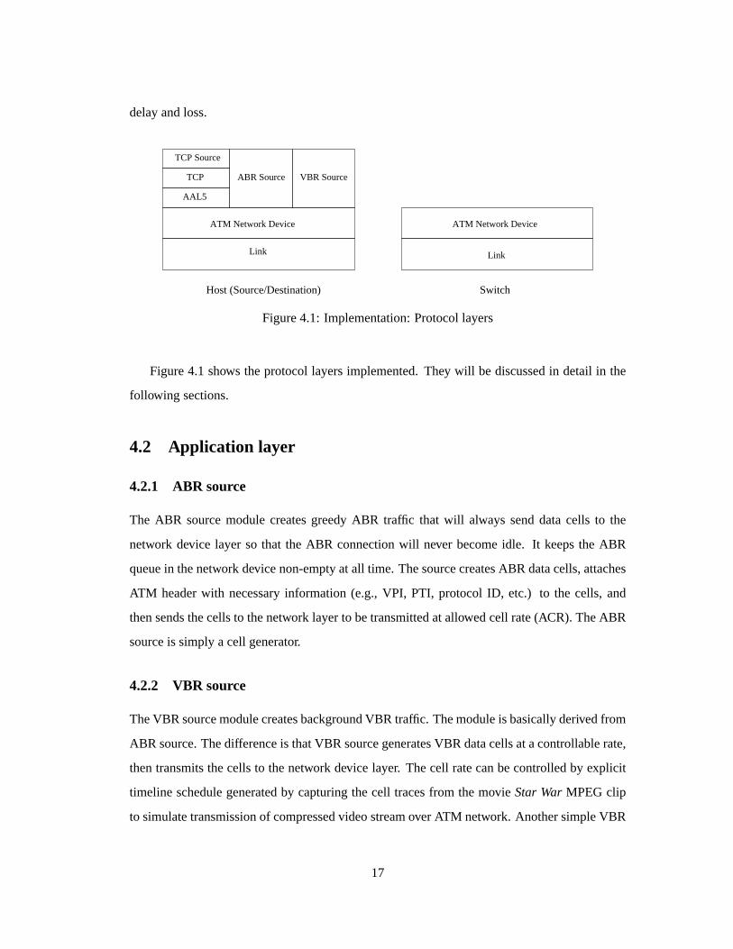
The implementationof ATM network andTCPtime warpsimulationmodelsaremodularized
basedon protocollayers. Protocollayersimplementedintegrateto form network components
suchasATM end-hostandswitch. Threesources:ABR source,VBR source,andTCPsource
with differenttraffic characteristicssimulatetheapplicationlayer. A TCPmodulesimulatesthe
transportlayer. A segmentationandreassembly(SAR)modulesimulatesATM AAL5 layer. An
ATM network module,which canbeviewedasanATM NIC device, simulatesATM network
services(i.e.,ABR, VBR) andmultiplexing. Finally, thereis a link modulethatfunctionsasthe
physicallink layer.
This approachprovidesan easyway in constructingnetwork scenarioespeciallyfor large
networks.Network scenarioconstructioncanadoptabottom-upapproachwherenetwork com-
ponentscanbeinterconnectedto form largernetwork. Also,network scenarioscanbemodified,
extended,andmaintainedat ease.However, theperformanceof this approachon GTW is not
known. Eachmodulerepresentsan LP in GTW. The complexity (e.g.,statesize,amountof
computationper event) of the LPs andthe patternof communicationamongLPs are factors
determiningGTW’s performance.This complex taskhasbeena researchissuein theparallel
simulationcommunityandit wouldbeleft asfuturework.
15
The focal pointsof this implementationaremodelcorrectness,compatibility to ProTEuS,
andoptimumexecutionon GTW. The developmentof eachmoduleis basedon the publicly
availableNISTATM simulator[16] sincethesimulatorperformscell-level ATM network sim-
ulation andis alsoevent-driven. The queuingstructure,ATM services,andevent scheduling
schemefrom theNIST simulatorareusedasa referencein this implementationto ensurecor-
rectnessof ATM simulationsdonein this work. Standardssuchas the ATM forum’s traffic
managementspecificationareanimportantsource.Themodulesdevelopedarealsotailoredto
matchthedesignof ProTEuSin termsof queueingdiscipline,ABR cell ratecontrolmechanis-
m, andotherATM functions.This ensurestheperformancecomparisonbetweenProTEuSand
GTW is fair becausethecomplexities of network modelsin bothplatformsarematching.
ATM technologyis calibratedto supporta broadspectrumof applicationsincluding loss-
sensitive data transmissionand the delay-sensitive real time audio and video transmission.
Hence,ATM layer provides four servicecategories: ConstantBit Rate(CBR), VariableBit
Rate(VBR), AvailableBit Rate(ABR), andUnspecifiedBit Rate(UBR). Theseservicecate-
goriesrelatetraffic characteristicsandQuality of Service(QoS)requirementsto network be-
havior. Eachservicecategory is associatedwith differentfunctionsfor routing,Call Admission
Control(CAC), andresourceallocation.
CBRapplicationsareguaranteedafixedamountof bandwidththroughoutthecourseof the
connection.This serviceis typically usedfor real-timeapplicationswith strict delayrequire-
ments. VBR serviceis intendedfor applicationswith bandwidthrequirementsthat vary with
time suchas interactive multimediaapplicationsand compressedvoice/videotransmissions.
VBR applicationsareguaranteeda sustainedcell rate in compliancewith a maximumburst
size. ABR serviceis aimedfor applicationswhosebandwidthrequirementscannotbe known
precisely, but areknown to bewithin anupperandlowerbound.ExampleABR applicationsare
FTPsessions,or Internettraffic. Theseapplicationsusestheinstantaneousavailablebandwidth
remainingafter all CBR andVBR traffic requirementshave beensatisfied.Thenetwork pro-
videsapplicationwith informationabouttheamountof availablebandwidththroughafeedback
system.EPRCAis onesuchfeedbacksystemthathasbeenimplementedin this work andwill
be discussedin detail later. Finally, UBR receives the remainingbandwithafter the previous
traffic classes.UBR is usedby best-effort services,suchase-mail, which are insensitive to
16
delayandloss.
VBR SourceABR Source
TCP Source
TCP
AAL5
ATM Network Device
Link
ATM Network Device
Link
Host (Source/Destination) Switch
Figure4.1: Implementation:Protocollayers
Figure4.1 shows theprotocollayersimplemented.They will bediscussedin detail in the
following sections.
4.2 Application layer
4.2.1 ABR source
The ABR sourcemodulecreatesgreedyABR traffic that will always senddatacells to the
network device layer so that the ABR connectionwill never becomeidle. It keepsthe ABR
queuein thenetwork devicenon-emptyatall time. ThesourcecreatesABR datacells,attaches
ATM headerwith necessaryinformation(e.g.,VPI, PTI, protocol ID, etc.) to the cells, and
thensendsthecellsto thenetwork layerto betransmittedatallowedcell rate(ACR).TheABR
sourceis simply acell generator.
4.2.2 VBR source
TheVBR sourcemodulecreatesbackgroundVBR traffic. Themoduleis basicallyderivedfrom
ABR source.Thedifferenceis thatVBR sourcegeneratesVBR datacellsatacontrollablerate,
thentransmitsthecells to thenetwork device layer. Thecell ratecanbecontrolledby explicit
timeline schedulegeneratedby capturingthecell tracesfrom themovie StarWar MPEG clip
to simulatetransmissionof compressedvideostreamoverATM network. AnothersimpleVBR
17
traffic generatorwe developedhasa squarewave transmissionpatternwith maximumcell rate,
minimumcell rate,andauser-definedduty cycle.
4.2.3 TCP source
A TCPsourceis alsoa greedysource.Note thatsourcesaredesignedto begreedysothat the
sourcewill alwaysfill up thebandwidthavailableto theconnection.Theaggregatetraffic from
all sourcescanbepredictedandhenceit is easierto control thebandwidthutilization of a link
in a network.
The TCP sourcesendsbuffers to the TCP layer and it will keepthe input buffer of the
TCPlayerbusysothattherearealwayspacketswaiting in theoutputbuffer of TCPlayerto be
propagatedto the lower protocol. A TCP connectionwill never becomeidle with this greedy
TCPsource.
4.3 TCP layer
TransmissionControlProtocol(TCP)offersaconnection-oriented, reliablebyte-streamservice.
It is a full-duplex protocol that guaranteesin-orderdelivery of a streamof bytes. EachTCP
connectionsupportsa pair of byte streams,oneflowing in eachdirection. It also includesa
window-basedflow-control mechanismfor a connectionthat allows the receiver to limit how
muchdatathesendercantransmit.
In additionto the above features,TCPalsoimplementsa highly tunedcongestioncontrol
mechanism.The ideaof this mechanismis to keepthesenderfrom overloadingthenetwork.
Thestrategy of congestioncontrol is for eachsourceto determinehow muchcapacityis avail-
able in the network, so that it knows how many packets it can safely have in transit in the
network. Oncea given sourcehasthis many packets in transit, it usesthe arrival of an ac-
knowledgement(ACK) asa signalthatoneof its packetshasreacheddestination,andthat it is
thereforesafeto insertanew packet into thenetwork without raisingthelevel of congestion.
To determinetheavailablecapacityin thenetwork, TCPusesanaggresive approachcalled
slow start to increasethe congestionwindow rapidly from a cold start. Congestionwindow
limits how many packetscanbe in transit in thenetwork. Thehigherthecongestionwindow,
18
the higher the throughput. Slowstart increasescongestionwindow exponentiallyuntil there
is a loss,at which time a timeoutcausesmultiplicative decrease.In otherwords,slow start
repeatedlyincreasesthe load it imposeson thenetwork in an effort to find thepoint at which
congestionoccurs,andthenit backsoff from thispoint.
Theoriginal implementationof TCPtimeoutsled to long periodsof time duringwhich the
connectionwentidle while waiting for a timer to expire. A new mechanismcalledfastretrans-
mit wasaddedto TCP. Themechanismtriggerstheretransmissionof a droppedpacket sooner
thantheregular timeoutmechanism.Whenthe fast retransmitmechanismsignalscongestion,
ratherthandropthecongestionwindowall thewaybackto 1 packetandrunslowstart, it is pos-
sibleto usetheACKs thatarestill in thepipeto clock thesendingof packets.This mechanism
called fast recovery removesthe slow start phasethat happensbetweenwhen fast retransmit
detectsa lost packet andadditive increasebegins. Slowstart is only usedat thebeginning of
a connectionandwhenever a regular long timeoutoccurs. At all othertimes, the congestion
windowis following apureadditive increase/multiplicative decreasepattern.
TheimplementedTCPlayeris a derivationof theBSD 4.3TCP(Renoversion)which will
behave asdescribedabove. TheTCPlayeralsosupportsdelayedACKs- acknowledgingevery
othersegmentratherthanevery segment- which is optional.
4.4 ATM Segmentationand Reassembly(SAR)
ATM cell is fixedatasizeof 53bytes.Packetshandeddown from high-level protocolareoften
larger than48 bytes,andthus,will not fit in thepayloadof anATM cell. Thesolutionto this
problemis to fragmentthehigh-level messageinto low-level packetsat thesource,transmitthe
individual packets over the network, andthenreassemblethe fragmentsback togetherat the
destination.Thetechniqueis calledsegmentationandreassembly(SAR).
TheATM AdaptationLayer(AAL) representsa SAR layer. AAL sitsbetweenATM layer
andthevariable-lengthpacketprotocolssuchasIP. SinceATM is designedto supportanumber
of services,differentserviceswould have differentAAL needs.Hence,four adaptationlayers
were originally defined. AAL1/2 were designedto supportguaranteedbit rate serviceslike
voice, while AAL3/4 were intendedto provide supportfor packet data transferover ATM.
AAL5 emergesasamoreefficient layeroverAAL3/4 andis thepreferredAAL in theIETF for
19
transmittingIP datagramsover ATM. AAL5 is implementedin this SAR modulesincewe are
assuminginternettraffic on theTCPconnections.
4.5 ATM network layer
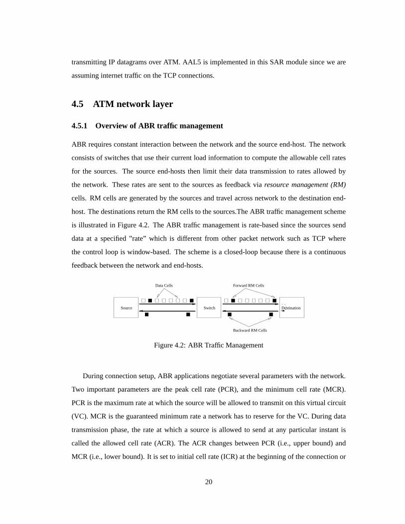
4.5.1 Overview of ABR traffic management
ABR requiresconstantinteractionbetweenthenetwork andthesourceend-host.Thenetwork
consistsof switchesthatusetheir currentloadinformationto computetheallowablecell rates
for the sources.The sourceend-hoststhen limit their datatransmissionto ratesallowed by
the network. Theseratesaresentto the sourcesasfeedbackvia resource management(RM)
cells. RM cellsaregeneratedby thesourcesandtravel acrossnetwork to thedestinationend-
host.ThedestinationsreturntheRM cellsto thesources.TheABR traffic managementscheme
is illustratedin Figure4.2. TheABR traffic managementis rate-basedsincethesourcessend
dataat a specified”rate” which is different from other packet network suchas TCP where
thecontrol loop is window-based.Theschemeis a closed-loopbecausethereis a continuous
feedbackbetweenthenetwork andend-hosts.
Data Cells
Source Switch Destination
Backward RM Cells
Forward RM Cells
Figure4.2: ABR Traffic Management
During connectionsetup,ABR applicationsnegotiateseveralparameterswith thenetwork.
Two importantparametersare the peakcell rate (PCR),and the minimum cell rate (MCR).
PCRis themaximumrateatwhich thesourcewill beallowedto transmiton thisvirtual circuit
(VC). MCR is theguaranteedminimumratea network hasto reserve for theVC. During data
transmissionphase,the rateat which a sourceis allowed to sendat any particularinstantis
called the allowed cell rate (ACR). The ACR changesbetweenPCR(i.e., upperbound)and
MCR (i.e., lower bound).It is setto initial cell rate(ICR) at thebeginningof theconnectionor
20
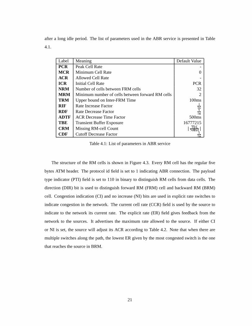
aftera long idle period. The list of parametersusedin theABR serviceis presentedin Table
4.1.
Label Meaning DefaultValuePCR PeakCell Rate -MCR Minimum Cell Rate 0ACR AllowedCell Rate -ICR Initial Cell Rate PCRNRM Numberof cellsbetweenFRM cells 32MRM Minimum numberof cellsbetweenforwardRM cells 2TRM Upperboundon Inter-FRM Time 100msRIF RateIncreaseFactor
����RDF RateDecreaseFactor
����ADTF ACR DecreaseTimeFactor 500msTBE TransientBuffer Exposure 16777215CRM MissingRM-cell Count
��������� ��CDF Cutoff DecreaseFactor
����Table4.1: List of parametersin ABR service
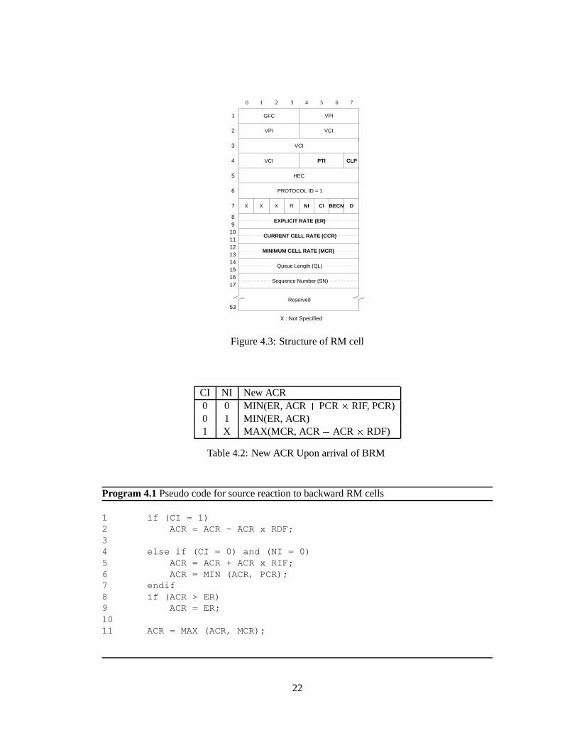
The structureof the RM cells is shown in Figure4.3. Every RM cell hasthe regular five
bytesATM header. The protocolid field is setto 1 indicatingABR connection.Thepayload
type indicator(PTI) field is setto 110 in binary to distinguishRM cells from datacells. The
direction(DIR) bit is usedto distinguishforward RM (FRM) cell andbackward RM (BRM)
cell. Congestionindication(CI) andno increase(NI) bits areusedin explicit rateswitchesto
indicatecongestionin thenetwork. Thecurrentcell rate(CCR)field is usedby thesourceto
indicateto the network its currentrate. The explicit rate (ER) field gives feedbackfrom the
network to the sources. It advertisesthe maximumrateallowed to the source. If eitherCI
or NI is set, the sourcewill adjustits ACR accordingto Table4.2. Note that whenthereare
multiple switchesalongthepath,thelowestER givenby themostcongestedswitchis theone
thatreachesthesourcein BRM.
21
0 1 2 3 4 5 6 7
X X X DR NI
1
2
3
4
5
6
7
8
10
12
14
16
9
11
13
15
17
EXPLICIT RATE (ER)
CURRENT CELL RATE (CCR)
Queue Length (QL)
Sequence Number (SN)
Reserved
PROTOCOL ID = 1
CLP
53
MINIMUM CELL RATE (MCR)
GFC
VPI
VPI
VCI
VCI
VCI PTI
HEC
CI
X : Not Specified
BECN
Figure4.3: Structureof RM cell
CI NI New ACR0 0 MIN(ER, ACR � PCR � RIF, PCR)0 1 MIN(ER, ACR)1 X MAX(MCR, ACR � ACR � RDF)
Table4.2: New ACR Uponarrival of BRM
Program 4.1Pseudocodefor sourcereactionto backwardRM cells
1 if (CI = 1)2 ACR = ACR - ACR x RDF;34 else if (CI = 0) and (NI = 0)5 ACR = ACR + ACR x RIF;6 ACR = MIN (ACR, PCR);7 endif8 if (ACR > ER)9 ACR = ER;1011 ACR = MAX (ACR, MCR);
22
4.5.2 ABR end-host
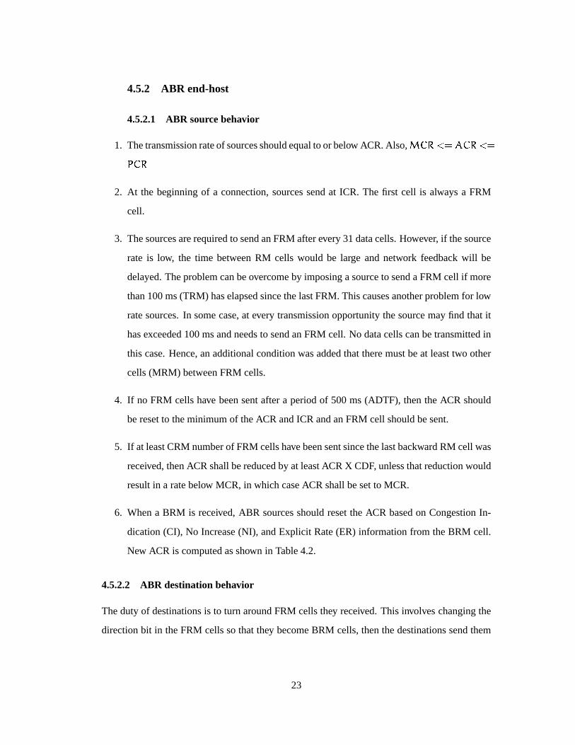
4.5.2.1 ABR sourcebehavior
1. Thetransmissionrateof sourcesshouldequaltoorbelow ACR.Also, ����������������� �! ���
2. At the beginning of a connection,sourcessendat ICR. The first cell is alwaysa FRM
cell.
3. Thesourcesarerequiredto sendanFRM afterevery31datacells.However, if thesource
rate is low, the time betweenRM cells would be large and network feedbackwill be
delayed.Theproblemcanbeovercomeby imposingasourceto sendaFRM cell if more
than100ms(TRM) haselapsedsincethelastFRM. Thiscausesanotherproblemfor low
ratesources.In somecase,at every transmissionopportunitythesourcemayfind that it
hasexceeded100msandneedsto sendanFRM cell. No datacellscanbetransmittedin
this case.Hence,anadditionalconditionwasaddedthat theremustbeat leasttwo other
cells(MRM) betweenFRM cells.
4. If no FRM cellshave beensentaftera periodof 500ms(ADTF), thentheACR should
beresetto theminimumof theACR andICR andanFRM cell shouldbesent.
5. If at leastCRM numberof FRM cellshavebeensentsincethelastbackwardRM cell was
received,thenACRshallbereducedby at leastACRX CDF, unlessthatreductionwould
resultin a ratebelow MCR, in whichcaseACR shallbesetto MCR.
6. Whena BRM is received,ABR sourcesshouldresettheACR basedon CongestionIn-
dication(CI), No Increase(NI), andExplicit Rate(ER) informationfrom theBRM cell.
New ACR is computedasshown in Table4.2.
4.5.2.2 ABR destinationbehavior
Theduty of destinationsis to turn aroundFRM cellsthey received. This involveschangingthe
directionbit in theFRM cellssothat they becomeBRM cells,thenthedestinationssendthem
23
backout on the VC on which they werereceived. The following items illustratedestination
behavior.
1. Whenadatacell is received, its EFCI bit is storedastheEFCI stateof theconnection.
2. Upon receiving FRM cell, the destinationshouldturn aroundthe cell to return to the
source.Thedirectionbit will bechangedfrom ”forward” to ”backward”. Also, settheCI
bit if theEFCI wassetin thelastdatacell received.
3. ABR destinationsmaysetCI and/orNI bits,aswell asmodifying theER in theRM cell
if it is experiencinginternalcongestion.
4. ABR destinationsmaygeneratea BRM cell without first having receiveda FRM cell in
order to increasethe responsivenessof the source. The Backward Explicit Congestion
Notification(BECN) andCI bit in theBRM cell shouldbeset.
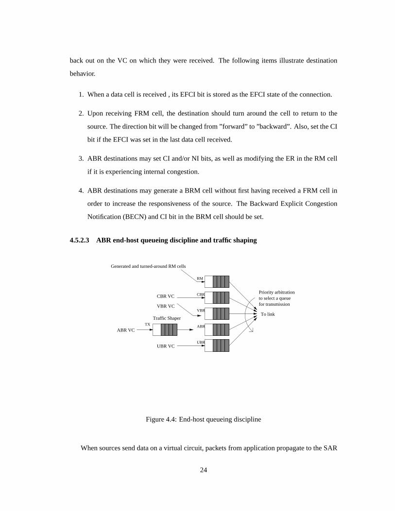
4.5.2.3 ABR end-hostqueueingdiscipline and traffic shaping
RM
CBR
VBR
ABR
UBR
Generated and turned-around RM cells
To link
ABR VC
Traffic Shaper
VBR VC
CBR VC
UBR VC
to select a queue Priority arbitration
for transmission
TX
Figure4.4: End-hostqueueingdiscipline
Whensourcessenddataonavirtual circuit, packetsfrom applicationpropagateto theSAR
24
layer wherethey arechoppedinto 48 byte payloads.Five bytesof ATM headerareaddedto
eachpayloadandastreamof 53 byteATM cellspropagateto thelower protocollayer.
Figure4.4 shows how ATM cells arequeuedat the ATM network device. Cells entering
ATM network layerarequeuedinto a transmitqueueon a per-VC basiswherethey wait to be
enabledby thetraffic shaper. Cell-level traffic shapingis performedon every ABR VC in this
implementation.The purposeof traffic shapingis to decidewhetheror not a VC shouldbe
allowed to senda cell basedon its currentcell rate(CCR).Thealgorithmof traffic shapingis
trivial. Theshaperspacescell transmissionon theVC asevenly aspossibleusingCCR.Each
ATM network device hasfive queuesasshown in Figure4.4. WhenABR cellsareenabledby
theshaper, they aretransferredfrom their VC queueto theABR queue.VBR traffics arenot
shapedandwill proceeddirectly to VBR queue.CBRandUBR queuesareunusedin thiswork.
At eachtransmissionopportunity, thenetwork device is allowedto sendonecell if they areany
in thedevice queues.Theschemeusedto choosea cell is a strict priority which favors traffic
classesin theorder:RM, CBR,VBR, ABR, andUBR. Hence,if anRM cell waiting, it will be
sentwith highestpriority, regardlessof theoccupancy of otherqueues.Theselectedcell is then
sentto thephysicallink.
4.5.3 Switch Behavior
4.5.3.1 Switch routing and queueingdiscipline
The taskof an ATM switch is to switch cells from an incoming(Port, VC) onto an outgoing
(Port,VC)basedon thecontentsof a routing table. Note that thecurrentimplementationdoes
not supportvirtual path(VPI) switchingcapabilities.Table4.3 shows a samplerouting table
with threeconnections.Eachentry representsrouting informationfor a particularconnection.
For instance,cells with VCI=1 comingfrom port number0 areroutedto port number6 with
sameVCI number.
The switch employs per-classqueueingdiscipline. In per-classqueueing,eachport hasa
FIFOqueuefor eachclassof traffic; CBR,VBR, ABR, andUBR. In addition,thereis aseparate
RM queueto segregateRM cells from datacells. As shown in Figure4.5, incomingcellsare
routedto theoutputport of their connectionwherethey arequeuedon theparticularqueuefor
their traffic class.
25
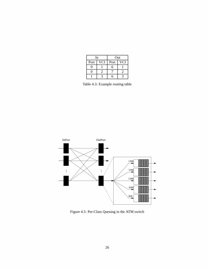
In OutPort VCI Port VCI
0 1 6 10 2 7 21 3 6 3
Table4.3: Exampleroutingtable
CBR
VBR
UBR
ABR
RM
...InPort
...
OutPort
Figure4.5: Per-ClassQueuingin theATM switch
26
Duringeachslottime,onecell fromeachportis transmittedtonext destination.A weighted-
roundrobin schedulingmechanismhasbeenimplementedto servicecellsbetweenclasseson
eachport. Sincethefocusof this work hasbeenABR serviceandbackgroundVBR traffic, the
schedulingsupportis only availablefor ABR andVBR. TheVBR andABR queuesareserviced
with a VBR:ABR weight ratio of 200:1. TheRM cells in theRM queueareservicedwith the
highestpriority.
4.5.3.2 Switch congestioncontrol
Despiteroutingcellsto their destination,theprinciplefunctionof ATM switchesis to monitor
congestionon theswitchesandprovide feedbackto theABR sources.Dueto theburstynature
of VBR traffic, theinstantaneousbandwidthavailableto ABR connectionsvarieswith timeand
maycausecongestionandcell loss.Theswitchesin anetwork shallreducecongestionandkeep
cell lossto minimumwhile efficiently allocatingthenetwork bandwidth.
Upon the receptionof a BRM cell, switchesinvoke a congestioncontrolalgorithmwhich
provides feedbackinformationto the ABR sourcesusingRM cells. Several congestioncon-
trol schemeshave beenproposedandthe two commonforms arebinary feedbacksystemand
explicit-ratefeedbacksystem.
Binary feedbacksystemis feedbackbasedonabinarycondition,normallyaflag to indicate
congestedor not congested. The Explicit Forward CongestionIndication (EFCI) bit in the
ATM headeris usedfor thispurpose.By settingtheEFCIbit, switchesonthepathfrom source
to destinationnotify the destinationthat congestionwasexperienced.Switchesmonitor their
queuelengthsandsetEFCIwhenthey exceededapredefinedthreshold.Sourcesrealizenetwork
congestionby observingtheEFCI bit in thereturningRM cells,thenthey adjusttheir sending
ratesusinganadditionalincrease/multiplicative decreasealgorithm.However, binaryschemes
canbeunfair sincethepenalizedsourcemaynotbetheonecausingthecongestion.
Explicit-rateschemesprovide sourceswith theactualratesat which to sendcells.Explicit-
rateschemesconverge fasterthanbinary schemesandthereforemoresuitablefor high speed
networks.Typicalexplicit-rateschemeperformsthefollowing:
1. Determineloadonswitchby eithermonitoringthequeuelengthor thequeuegrowth rate.
2. Computethefair shareof thebandwidthfor eachVC thatcanbesupported.
27
3. Determinetheexplicit ratesandsendtheseinformationto thesourcesthroughRM cells.
Examplesof explicit rateschemesaretheEnhancedProportionalRateControlAlgorithm
(EPRCA)andExplicit RateIndicationfor CongestionAvoidance(ERICA).
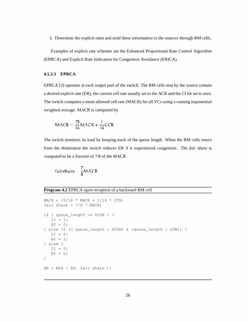
4.5.3.3 EPRCA
EPRCA[3] operatesateachoutputportof theswitch.TheRM cellssentby thesourcecontain
adesiredexplicit rate(ER),thecurrentcell rateusuallysetto theACRandtheCI bit setto zero.
Theswitchcomputesameanallowedcell rate(MACR)for all VCsusingarunningexponential
weightedaverage.MACR is computedby
�"�������#%$#'& �"�����(�
##'& �)���
Theswitchmonitorsits loadby keepingtrackof thequeuelength. WhentheRM cells return
from the destinationthe switch reducesER if it experiencedcongestion. The fair share is
computedto bea fractionof 7/8of theMACR
*,+.-0/'132�+./�4 �56 �"�����
Program 4.2EPRCAuponreceptionof abackwardRM cell
MACR = 15/16 * MACR + 1/16 * CCR;fair share = 7/8 * MACR;
if ( queue_length >= HIGH ) {CI = 1;NI = 0;
} else if (( queue_length < HIGH) & (queue_length > LOW)) {CI = 0;NI = 1;
} else {CI = 0;NI = 0;
}
ER = MIN ( ER, fair share );
28
Program4.2showstheoperationof EPRCAatthereceptionof aBRM cell. EPRCAsetsthe
CI andNI bitsbasedontheABR queuelengthof theportonwhichtheBRM cell wasreceived.
Thevalueof LOW andHIGH thresholdsaresetto 200cellsand300cellsrespectively.
If the calculatedfair share is greaterthanER value in the BRM cell, thenthe ER is un-
changed,otherwisetheERis setto thefair share. Thisensuresthatif BRM cell traversesmore
thanoneswitch, theminimumof the fair share reachesthesource.Thusavoidscongestionat
thebottlenectswitch.
EPRCAis generallya congestionreactionschemewhich is computationallysimple.How-
ever, its congestiondetectionmechanism,whichis basedonqueuelength,hasbeenshown to be
unfair. A betterapproachis ERICA, a congestionavoidanceschemewhich usedqueuegrowth
rateasloadindicator. ERICA is not implementedandhencewill notbediscussedhere.
29
Chapter 5
Evaluation
5.1 Overview
Thischapterevaluatesandcomparestheperformanceof GTW to ProTEuSin termsof speedup,
scalability on network size, as well as the impact of network characteristicsand simulation
parameters.The next sectionvalidatesthe network modulesimplemented.A fairly complex
topologyis usedto generatedetail network resultsto be comparedto thoseof ProTEuS.This
ensurescorrectsimulationresults.Therestof thesectionsfocuson large-scaleATM network
topologiesin performingfurtherperformancestudy.
Experimentsin thischapterwereperformedonan8-processorSunEnterpriseserverknown
asClipper locatedat the LawrenceBerkeley NationalLaboratory. Importantinformationon
Clipper is listedin Table5.1
Nodename ClipperPlatform SUN Ultra-EnterpriseOperatingSystem SunOS5.7Numberof CPU 8CPUclock speed 168MHz
Table5.1: Clippersysteminformation
30
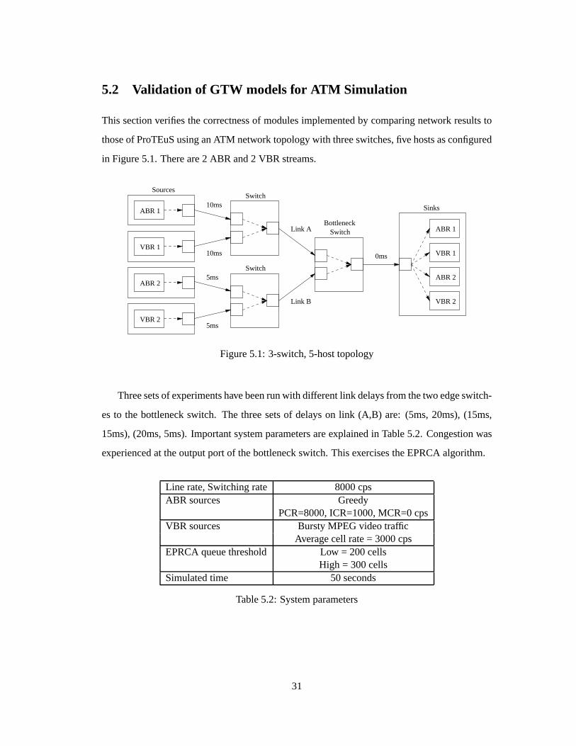
5.2 Validation of GTW modelsfor ATM Simulation
This sectionverifiesthecorrectnessof modulesimplementedby comparingnetwork resultsto
thoseof ProTEuSusinganATM network topologywith threeswitches,fivehostsasconfigured
in Figure5.1.Thereare2 ABR and2 VBR streams.
ABR 1
VBR 1
ABR 2
VBR 2
ABR 1
VBR 1
ABR 2
VBR 2
Switch
Switch
SwitchLink A
Link B
10ms
5ms
10ms
5ms
Bottleneck
Sources
Sinks
0ms
Figure5.1: 3-switch,5-hosttopology
Threesetsof experimentshavebeenrunwith differentlink delaysfrom thetwo edgeswitch-
esto the bottleneckswitch. The threesetsof delayson link (A,B) are: (5ms,20ms),(15ms,
15ms),(20ms,5ms). Importantsystemparametersareexplainedin Table5.2. Congestionwas
experiencedat theoutputportof thebottleneckswitch.ThisexercisestheEPRCAalgorithm.
Line rate,Switchingrate 8000cpsABR sources Greedy
PCR=8000,ICR=1000,MCR=0cpsVBR sources BurstyMPEGvideotraffic
Averagecell rate= 3000cpsEPRCAqueuethreshold Low = 200cells
High = 300cellsSimulatedtime 50 seconds
Table5.2: Systemparameters
31
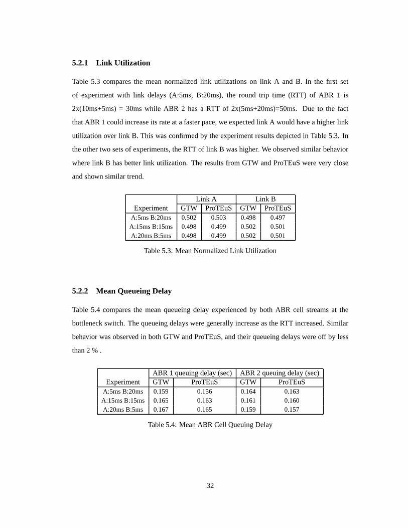
5.2.1 Link Utilization
Table 5.3 comparesthe meannormalizedlink utilizations on link A and B. In the first set
of experimentwith link delays(A:5ms, B:20ms), the round trip time (RTT) of ABR 1 is
2x(10ms+5ms)= 30mswhile ABR 2 hasa RTT of 2x(5ms+20ms)=50ms.Due to the fact
thatABR 1 couldincreaseits rateata fasterpace,weexpectedlink A wouldhave ahigherlink
utilization over link B. This wasconfirmedby theexperimentresultsdepictedin Table5.3. In
theothertwo setsof experiments,theRTT of link B washigher. Weobservedsimilar behavior
wherelink B hasbetterlink utilization. Theresultsfrom GTW andProTEuSwerevery close
andshown similar trend.
Link A Link BExperiment GTW ProTEuS GTW ProTEuS
A:5msB:20ms 0.502 0.503 0.498 0.497A:15msB:15ms 0.498 0.499 0.502 0.501A:20msB:5ms 0.498 0.499 0.502 0.501
Table5.3: MeanNormalizedLink Utilization
5.2.2 Mean QueueingDelay
Table 5.4 comparesthe meanqueueingdelay experiencedby both ABR cell streamsat the
bottleneckswitch. ThequeueingdelaysweregenerallyincreaseastheRTT increased.Similar
behavior wasobserved in bothGTW andProTEuS,andtheir queueingdelayswereoff by less
than2 % .
ABR 1 queuingdelay(sec) ABR 2 queuingdelay(sec)Experiment GTW ProTEuS GTW ProTEuS
A:5msB:20ms 0.159 0.156 0.164 0.163A:15msB:15ms 0.165 0.163 0.161 0.160A:20msB:5ms 0.167 0.165 0.159 0.157
Table5.4: MeanABR Cell QueuingDelay
32
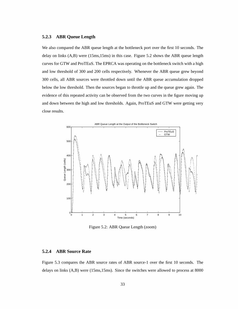
5.2.3 ABR QueueLength
We alsocomparedtheABR queuelengthat thebottleneckport over thefirst 10 seconds.The
delayon links (A,B) were(15ms,15ms)in this case.Figure5.2 shows theABR queuelength
curvesfor GTW andProTEuS.TheEPRCAwasoperatingonthebottleneckswitchwith ahigh
andlow thresholdof 300 and200 cells respectively. Whenever the ABR queuegrew beyond
300 cells, all ABR sourceswere throttleddown until the ABR queueaccumulationdropped
below thelow threshold.Thenthesourcesbeganto throttleup andthequeuegrew again.The
evidenceof this repeatedactivity canbeobservedfrom thetwo curvesin thefiguremoving up
anddown betweenthehigh andlow thresholds.Again, ProTEuSandGTW weregettingvery
closeresults.
0 1 2 3 4 5 6 7 8 9 100
100
200
300
400
500
600ABR Queue Length at the Output of the Bottleneck Switch
Time (seconds)
Que
ue L
engt
h (c
ells
)
ProTEuSGTW
Figure5.2: ABR QueueLength(zoom)
5.2.4 ABR SourceRate
Figure5.3 comparesthe ABR sourceratesof ABR source-1over the first 10 seconds.The
delayson links (A,B) were(15ms,15ms).Sincetheswitcheswereallowed to processat 8000
33
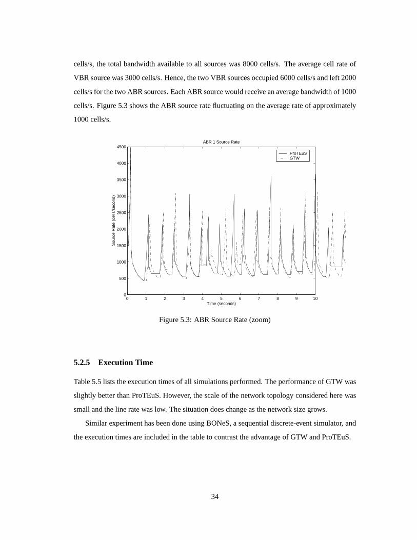
cells/s,the total bandwidthavailableto all sourceswas8000cells/s. The averagecell rateof
VBR sourcewas3000cells/s.Hence,thetwo VBR sourcesoccupied6000cells/sandleft 2000
cells/sfor thetwo ABR sources.EachABR sourcewouldreceiveanaveragebandwidthof 1000
cells/s.Figure5.3shows theABR sourceratefluctuatingon theaveragerateof approximately
1000cells/s.
0 1 2 3 4 5 6 7 8 9 100
500
1000
1500
2000
2500
3000
3500
4000
4500ABR 1 Source Rate
Sou
rce
Rat
e (c
ells
/sec
ond)
Time (seconds)
ProTEuSGTW
Figure5.3: ABR SourceRate(zoom)
5.2.5 ExecutionTime
Table5.5 lists theexecutiontimesof all simulationsperformed.Theperformanceof GTW was
slightly betterthanProTEuS.However, thescaleof thenetwork topologyconsideredherewas
smallandtheline ratewaslow. Thesituationdoeschangeasthenetwork sizegrows.
Similar experimenthasbeendoneusingBONeS,asequentialdiscrete-eventsimulator, and
theexecutiontimesareincludedin thetableto contrasttheadvantageof GTW andProTEuS.
34
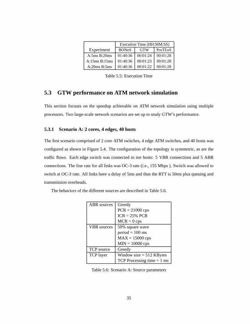
ExecutionTime(HH:MM:SS)Experiment BONeS GTW ProTEuS
A:5msB:20ms 01:40:36 00:01:24 00:01:28A:15msB:15ms 01:40:36 00:01:23 00:01:28A:20msB:5ms 01:40:36 00:01:22 00:01:28
Table5.5: ExecutionTime
5.3 GTW performanceon ATM network simulation
This sectionfocuseson the speedupachievable on ATM network simulationusing multiple
processors.Two large-scalenetwork scenariosaresetup to studyGTW’sperformance.
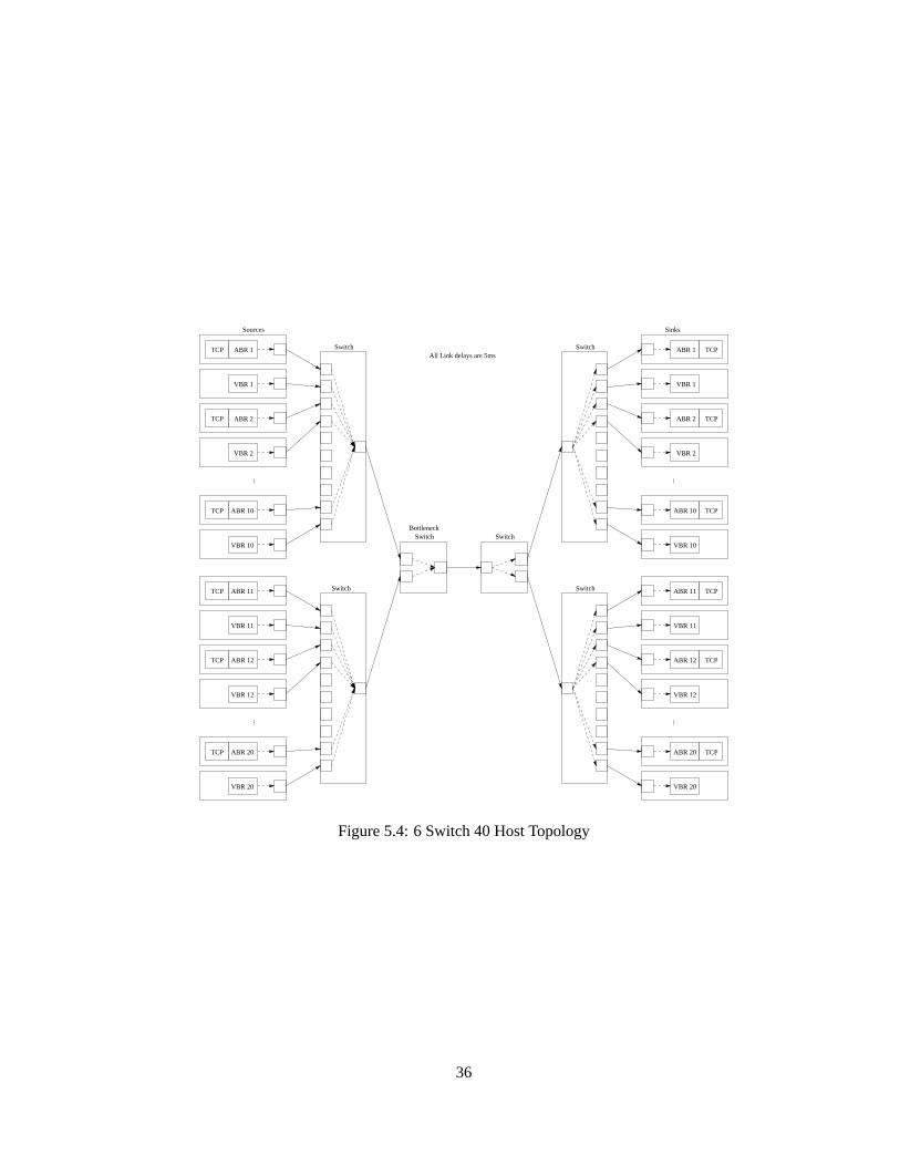
5.3.1 ScenarioA: 2 cores,4 edges,40hosts
Thefirst scenariocomprisedof 2 coreATM switches,4 edgeATM switches,and40 hostswas
configuredasshown in Figure5.4. Theconfigurationof thetopologyis symmetric,asarethe
traffic flows. Eachedgeswitch wasconnectedto ten hosts: 5 VBR connectionsand5 ABR
connections.Theline ratefor all links wasOC-3rate(i.e.,155Mbps). Switchwasallowedto
switchat OC-3rate.All links have a delayof 5msandthustheRTT is 50msplusqueuingand
transmissionoverheads.
Thebehaviors of thedifferentsourcesaredescribedin Table5.6.
ABR sources GreedyPCR= 21000cpsICR = 25%PCRMCR = 0 cps
VBR sources 50%squarewaveperiod= 100msMAX = 15000cpsMIN = 10000cps
TCPsource GreedyTCPlayer Window size= 512KBytes
TCPProcessingtime= 1 ms
Table5.6: ScenarioA: Sourceparameters
35
ABR 1
VBR 1
ABR 2
VBR 2
VBR 10
ABR 11
VBR 11
ABR 12
VBR 12
ABR 20
VBR 20 VBR 20
ABR 20
VBR 12
ABR 12
ABR 11
VBR 11
VBR 10
ABR 10
VBR 2
ABR 2
VBR 1
ABR 1TCP
TCP
TCP
TCP
TCP
TCP TCP
TCP
TCP
TCP
TCP
TCP
ABR 10
Switch
Sources
......
Switch
Switch
SwitchBottleneck
Switch
Switch
Sinks
......
All Link delays are 5ms
Figure5.4: 6 Switch40 HostTopology
36
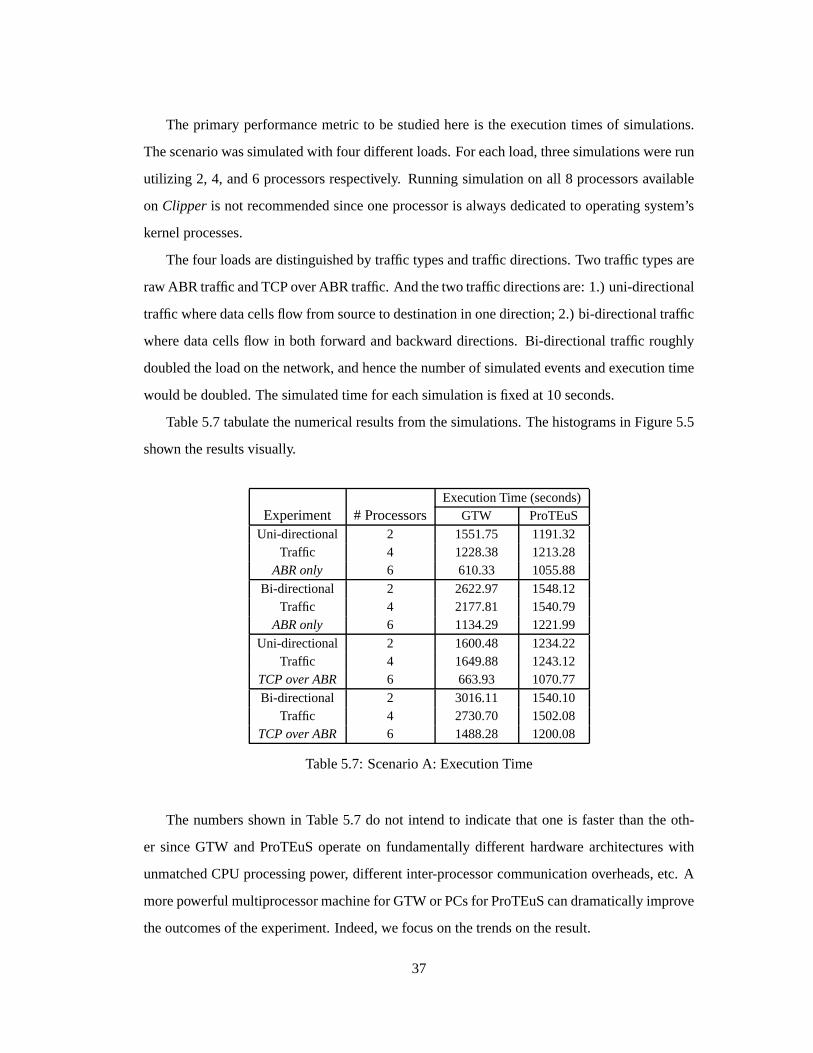
The primary performancemetric to be studiedhereis the executiontimesof simulations.
Thescenariowassimulatedwith four differentloads.For eachload,threesimulationswererun
utilizing 2, 4, and6 processorsrespectively. Runningsimulationon all 8 processorsavailable
on Clipper is not recommendedsinceoneprocessoris alwaysdedicatedto operatingsystem’s
kernelprocesses.
Thefour loadsaredistinguishedby traffic typesandtraffic directions.Two traffic typesare
raw ABR traffic andTCPoverABR traffic. And thetwo traffic directionsare:1.) uni-directional
traffic wheredatacellsflow from sourceto destinationin onedirection;2.) bi-directionaltraffic
wheredatacells flow in both forward andbackward directions. Bi-directionaltraffic roughly
doubledtheloadon thenetwork, andhencethenumberof simulatedeventsandexecutiontime
wouldbedoubled.Thesimulatedtime for eachsimulationis fixedat 10seconds.
Table5.7 tabulatethenumericalresultsfrom thesimulations.Thehistogramsin Figure5.5
shown theresultsvisually.
ExecutionTime(seconds)Experiment # Processors GTW ProTEuS
Uni-directional 2 1551.75 1191.32Traffic 4 1228.38 1213.28
ABRonly 6 610.33 1055.88
Bi-directional 2 2622.97 1548.12Traffic 4 2177.81 1540.79
ABRonly 6 1134.29 1221.99
Uni-directional 2 1600.48 1234.22Traffic 4 1649.88 1243.12
TCPoverABR 6 663.93 1070.77
Bi-directional 2 3016.11 1540.10Traffic 4 2730.70 1502.08
TCPoverABR 6 1488.28 1200.08
Table5.7: ScenarioA: ExecutionTime
The numbersshown in Table5.7 do not intendto indicatethat oneis fasterthanthe oth-
er sinceGTW andProTEuSoperateon fundamentallydifferent hardware architectureswith
unmatchedCPUprocessingpower, differentinter-processorcommunicationoverheads,etc. A
morepowerful multiprocessormachinefor GTW or PCsfor ProTEuScandramaticallyimprove
theoutcomesof theexperiment.Indeed,we focuson thetrendson theresult.
37
2 4 60
500
1000
1500
2000
2500
3000
3500Uni−ABR
Num. CPU
Exe
c. ti
me
(sec
onds
)
GTW ProTEuS
2 4 60
500
1000
1500
2000
2500
3000
3500Bi−ABR
Num. CPU
Exe
c. ti
me
(sec
onds
)2 4 6
0
500
1000
1500
2000
2500
3000
3500Uni−TCP/ABR
Num. CPU
Exe
c. ti
me
(sec
onds
)
2 4 60
500
1000
1500
2000
2500
3000
3500Bi−TCP/ABR
Num. CPUE
xec.
tim
e (s
econ
ds)
Figure5.5: ScenarioA: Executiontimevs NumberCPU
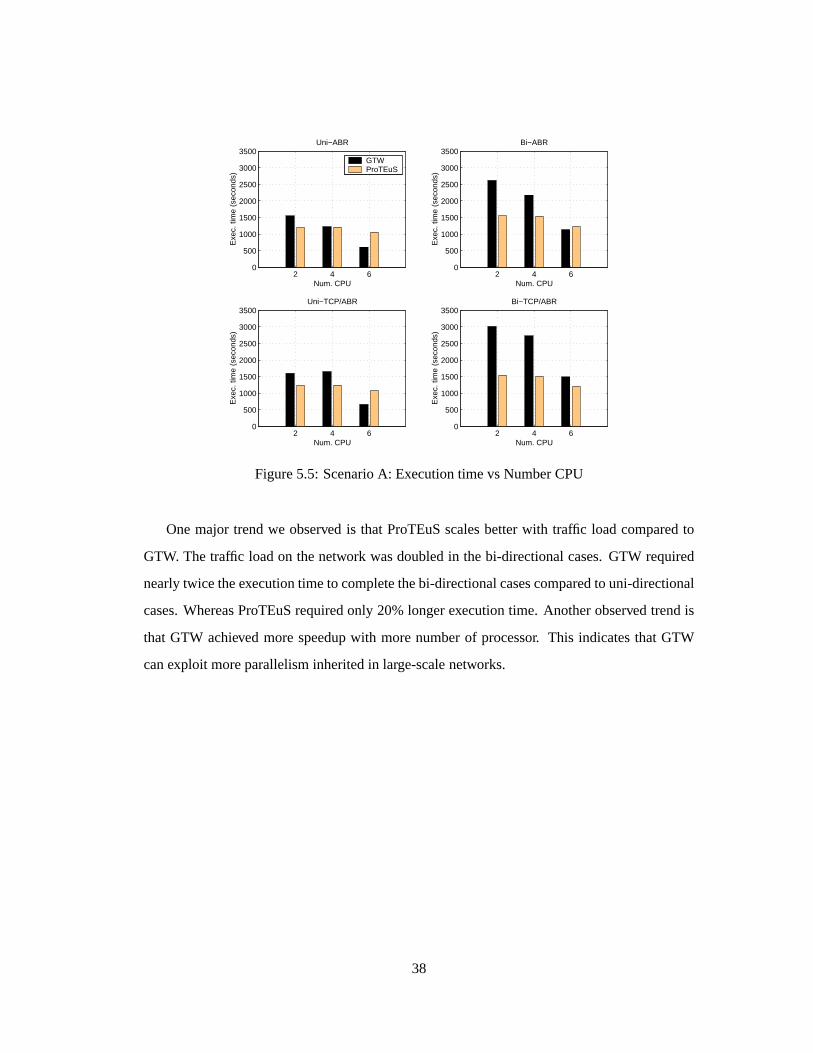
Onemajor trendwe observed is that ProTEuSscalesbetterwith traffic load comparedto
GTW. Thetraffic loadon thenetwork wasdoubledin thebi-directionalcases.GTW required
nearlytwicetheexecutiontimeto completethebi-directionalcasescomparedto uni-directional
cases.WhereasProTEuSrequiredonly 20%longerexecutiontime. Anotherobservedtrendis
that GTW achieved morespeedupwith morenumberof processor. This indicatesthat GTW
canexploit moreparallelisminheritedin large-scalenetworks.
38
1 1.5 2 2.5 3 3.5 4 4.5 5 5.5 61
1.5
2
2.5
3
3.5Speedup vs # Processors ( Scenario A )
Num. Processor
Spe
edup
Uni−ABR Uni−TCP/ABRBi−ABR Bi−TCP/ABR
Figure5.6: ScenarioA: GTW Speedup(relative to 1 processor)
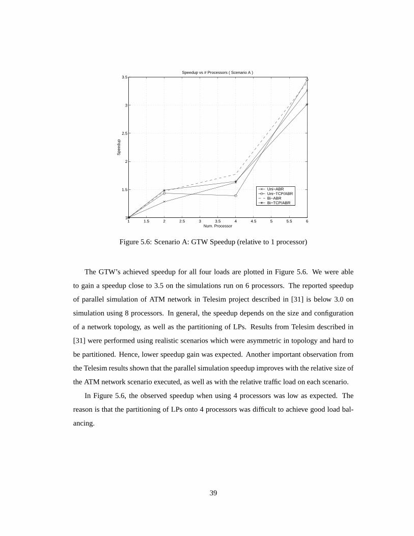
The GTW’s achieved speedupfor all four loadsareplotted in Figure5.6. We wereable
to gain a speedupcloseto 3.5 on the simulationsrun on 6 processors.The reportedspeedup
of parallel simulationof ATM network in Telesimprojectdescribedin [31] is below 3.0 on
simulationusing8 processors.In general,thespeedupdependson thesizeandconfiguration
of a network topology, aswell asthe partitioningof LPs. Resultsfrom Telesimdescribedin
[31] wereperformedusingrealisticscenarioswhich wereasymmetricin topologyandhardto
bepartitioned.Hence,lower speedupgainwasexpected.Anotherimportantobservation from
theTelesimresultsshown thattheparallelsimulationspeedupimproveswith therelativesizeof
theATM network scenarioexecuted,aswell aswith therelative traffic loadoneachscenario.
In Figure5.6, the observed speedupwhenusing4 processorswaslow asexpected. The
reasonis that thepartitioningof LPsonto4 processorswasdifficult to achieve goodloadbal-
ancing.
39
5.3.2 ScenarioB: 4 cores,12 edges,120hosts
TCP ABR
VBR
TCP ABR
VBR...
...
Sources
Edge Switch
TCP ABR
VBR
TCP ABR
VBR
......
Sources
Edge Switch
TCP ABR
VBR
TCP ABR
VBR
......
Sources
Edge Switch
TCP ABR
VBR
TCP ABR
VBR
......
Sources
Edge Switch
TCP ABR
VBR
TCP ABR
VBR
......
Sources
Edge Switch
TCP ABR
VBR
TCP ABR
VBR
......
Sources
Edge Switch
......
ABR
VBR
TCP
ABR TCP
VBR
Edge Switch
Sources
......
ABR
VBR
TCP
ABR TCP
VBR
Edge Switch
Sources
......
ABR
VBR
TCP
ABR TCP
VBR
Edge Switch
Sources
......
ABR
VBR
TCP
ABR TCP
VBR
Edge Switch
Sources
......
ABR
VBR
TCP
ABR TCP
VBR
Edge Switch
Sources
......
ABR
VBR
TCP
ABR TCP
VBR
Edge Switch
Sources
Core SwitchCore Switch
Core SwitchCore Switch
Figure5.7: 16 Switch120HostTopology
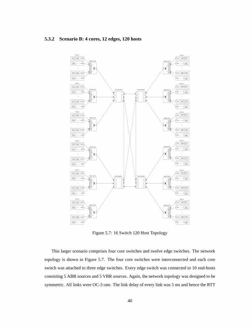
This largerscenariocomprisesfour coreswitchesandtwelve edgeswitches.Thenetwork
topology is shown in Figure5.7. The four coreswitcheswere interconnectedandeachcore
switchwasattachedto threeedgeswitches.Every edgeswitchwasconnectedto 10 end-hosts
consisting5 ABR sourcesand5 VBR sources.Again,thenetwork topologywasdesignedto be
symmetric.All links wereOC-3rate.Thelink delayof every link was5 msandhencetheRTT
40
of all connectionswas50 ms.
Thebehaviors of thedifferentsourcesaredescribedin Table5.8.
ABR sources GreedyPCR= 36000cpsICR = 25%PCRMCR = 0 cps
VBR sources 50%squarewaveperiod= 100msMAX = 36000cpsMIN = 10000cps
TCPsource GreedyTCPlayer Window size= 128KBytes
TCPProcessingtime= 1 ms
Table5.8: ScenarioB: Sourceparameters
Simulationswith different loadsthat have beenperformedon the previous scenariowere
repeatedon this scenario.Theonly changemadewasthat we reducedthesimulatedfrom 10
secondsto 1 second.Thereducedsimulatedtimewouldstill yield stableresultssincethis larger
scenariowould executeapproximatelysix timesmoreeventsthanthepreviousscenario.Table
5.9tabulatesthenumericalresultsfrom thesimulations.Thehistogramsin Figure5.8compared
theresultsvisually.
41
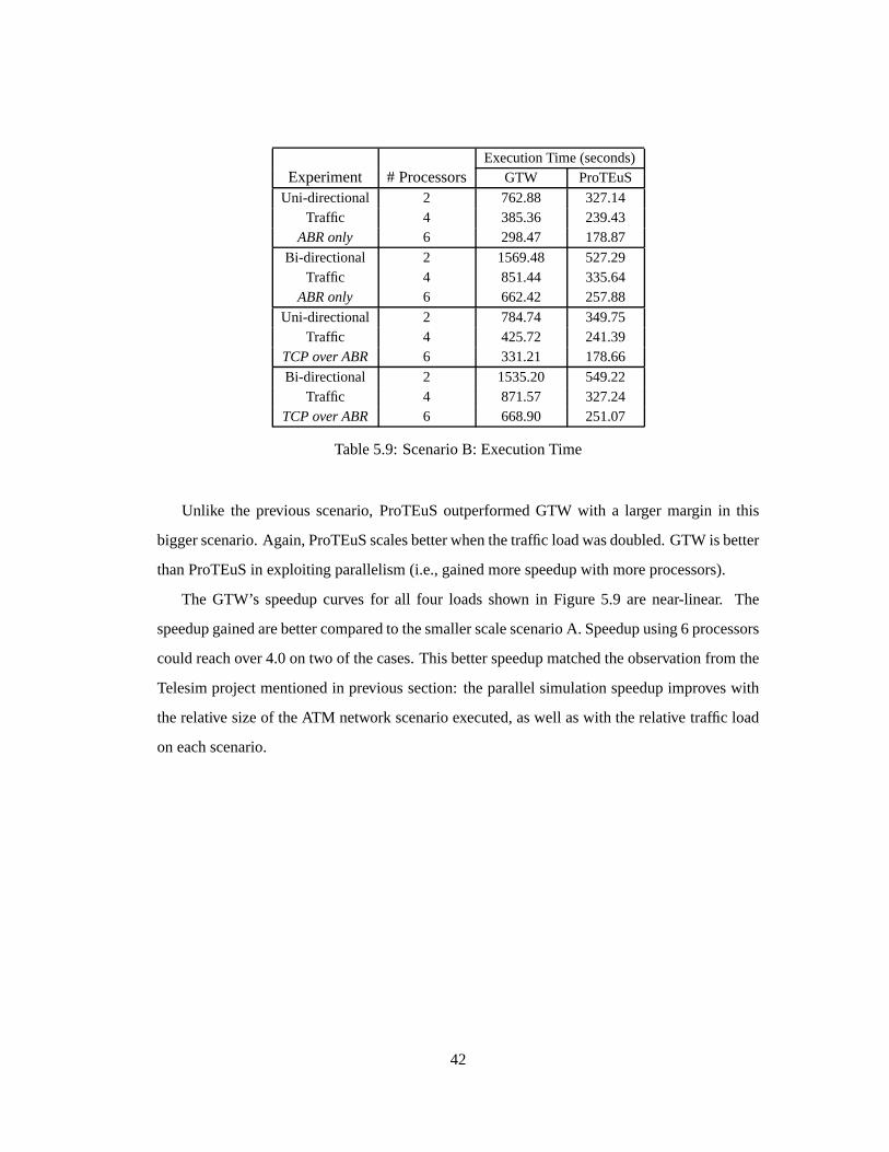
ExecutionTime(seconds)Experiment # Processors GTW ProTEuS
Uni-directional 2 762.88 327.14Traffic 4 385.36 239.43
ABRonly 6 298.47 178.87
Bi-directional 2 1569.48 527.29Traffic 4 851.44 335.64
ABRonly 6 662.42 257.88
Uni-directional 2 784.74 349.75Traffic 4 425.72 241.39
TCPoverABR 6 331.21 178.66
Bi-directional 2 1535.20 549.22Traffic 4 871.57 327.24
TCPoverABR 6 668.90 251.07
Table5.9: ScenarioB: ExecutionTime
Unlike the previous scenario,ProTEuSoutperformedGTW with a larger margin in this
biggerscenario.Again,ProTEuSscalesbetterwhenthetraffic loadwasdoubled.GTW is better
thanProTEuSin exploiting parallelism(i.e.,gainedmorespeedupwith moreprocessors).
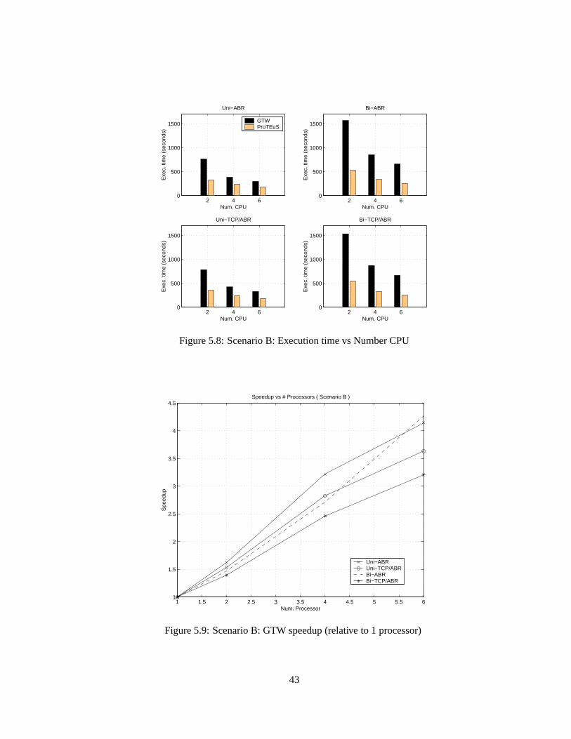
The GTW’s speedupcurves for all four loadsshown in Figure 5.9 are near-linear. The
speedupgainedarebettercomparedto thesmallerscalescenarioA. Speedupusing6 processors
couldreachover4.0ontwo of thecases.Thisbetterspeedupmatchedtheobservationfrom the
Telesimprojectmentionedin previous section:theparallelsimulationspeedupimproveswith
therelative sizeof theATM network scenarioexecuted,aswell aswith therelative traffic load
on eachscenario.
42
2 4 60
500
1000
1500
Uni−ABR
Num. CPU
Exe
c. ti
me
(sec
onds
)
GTW ProTEuS
2 4 60
500
1000
1500
Bi−ABR
Num. CPU
Exe
c. ti
me
(sec
onds
)2 4 6
0
500
1000
1500
Uni−TCP/ABR
Num. CPU
Exe
c. ti
me
(sec
onds
)
2 4 60
500
1000
1500
Bi−TCP/ABR
Num. CPU
Exe
c. ti
me
(sec
onds
)
Figure5.8: ScenarioB: Executiontimevs NumberCPU
1 1.5 2 2.5 3 3.5 4 4.5 5 5.5 61
1.5
2
2.5
3
3.5
4
4.5Speedup vs # Processors ( Scenario B )
Num. Processor
Spe
edup
Uni−ABR Uni−TCP/ABRBi−ABR Bi−TCP/ABR
Figure5.9: ScenarioB: GTW speedup(relative to 1 processor)
43
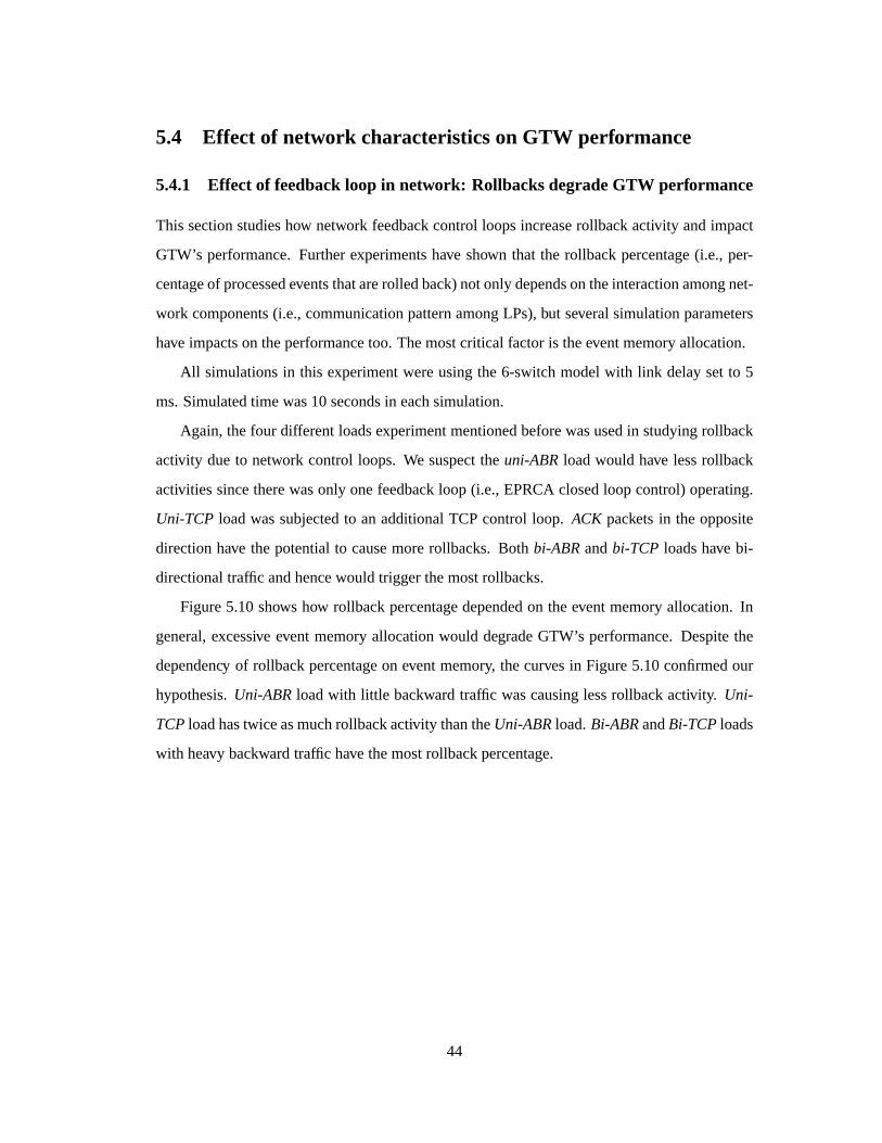
5.4 Effect of network characteristicson GTW performance
5.4.1 Effect of feedbackloop in network: RollbacksdegradeGTW performance
This sectionstudieshow network feedbackcontrol loopsincreaserollbackactivity andimpact
GTW’s performance.Furtherexperimentshave shown that the rollback percentage(i.e., per-
centageof processedeventsthatarerolledback)notonly dependsontheinteractionamongnet-
work components(i.e., communicationpatternamongLPs),but severalsimulationparameters
have impactson theperformancetoo. Themostcritical factoris theeventmemoryallocation.
All simulationsin this experimentwereusingthe6-switchmodelwith link delaysetto 5
ms.Simulatedtime was10 secondsin eachsimulation.
Again, thefour differentloadsexperimentmentionedbeforewasusedin studyingrollback
activity dueto network control loops. We suspecttheuni-ABRloadwould have lessrollback
activities sincetherewasonly onefeedbackloop (i.e., EPRCAclosedloop control)operating.
Uni-TCP loadwassubjectedto an additionalTCPcontrol loop. ACK packets in theopposite
directionhave thepotentialto causemorerollbacks. Both bi-ABRandbi-TCP loadshave bi-
directionaltraffic andhencewould triggerthemostrollbacks.
Figure5.10shows how rollbackpercentagedependedon theeventmemoryallocation. In
general,excessive event memoryallocationwould degradeGTW’s performance.Despitethe
dependency of rollbackpercentageon eventmemory, thecurvesin Figure5.10confirmedour
hypothesis.Uni-ABR loadwith little backward traffic wascausinglessrollbackactivity. Uni-
TCPloadhastwiceasmuchrollbackactivity thantheUni-ABRload.Bi-ABRandBi-TCPloads
with heavy backwardtraffic have themostrollbackpercentage.
44
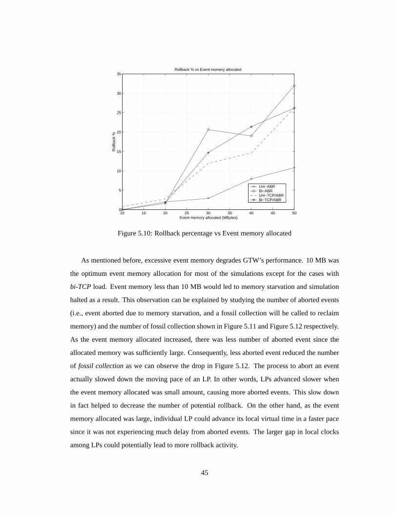
10 15 20 25 30 35 40 45 500
5
10
15
20
25
30
35Rollback % vs Event momery allocated
Event memory allocated (MBytes)
Rol
lbac
k %
Uni−ABR Bi−ABR Uni−TCP/ABRBi−TCP/ABR
Figure5.10:RollbackpercentagevsEventmemoryallocated
As mentionedbefore,excessive eventmemorydegradesGTW’s performance.10 MB was
the optimumevent memoryallocationfor mostof the simulationsexcept for the caseswith
bi-TCP load. Eventmemorylessthan10 MB would led to memorystarvationandsimulation
haltedasa result.This observationcanbeexplainedby studyingthenumberof abortedevents
(i.e., eventaborteddueto memorystarvation,anda fossil collectionwill be calledto reclaim
memory)andthenumberof fossilcollectionshown in Figure5.11andFigure5.12respectively.
As the event memoryallocatedincreased,therewas lessnumberof abortedevent sincethe
allocatedmemorywassufficiently large. Consequently, lessabortedeventreducedthenumber
of fossil collectionaswe canobserve the drop in Figure5.12. The processto abortan event
actuallyslowed down the moving paceof an LP. In otherwords,LPs advancedslower when
theeventmemoryallocatedwassmallamount,causingmoreabortedevents. This slow down
in fact helpedto decreasethe numberof potentialrollback. On the otherhand,as the event
memoryallocatedwaslarge,individual LP couldadvanceits local virtual time in a fasterpace
sinceit wasnot experiencingmuchdelayfrom abortedevents. The larger gapin local clocks
amongLPscouldpotentiallyleadto morerollbackactivity.
45

10 15 20 25 30 35 40 45 500
0.5
1
1.5
2
2.5
3x 10
5 Number of Aborted event vs Event momery allocated
Event memory allocated (MBytes)
Num
ber
of A
bort
ed e
vent
Uni−ABR Bi−ABR Uni−TCP/ABRBi−TCP/ABR
Figure5.11:Numberof abortedeventvs Eventmemoryallocated
10 15 20 25 30 35 40 45 500
0.5
1
1.5
2
2.5
3
3.5
4
4.5x 10
4 Number of Fossil Collection vs Event momery allocated
Event memory allocated (MBytes)
Num
ber
of F
ossi
l Col
lect
ion
Uni−ABR Bi−ABR Uni−TCP/ABRBi−TCP/ABR
Figure5.12:Numberof fossil collectionvsEventmemoryallocated
46
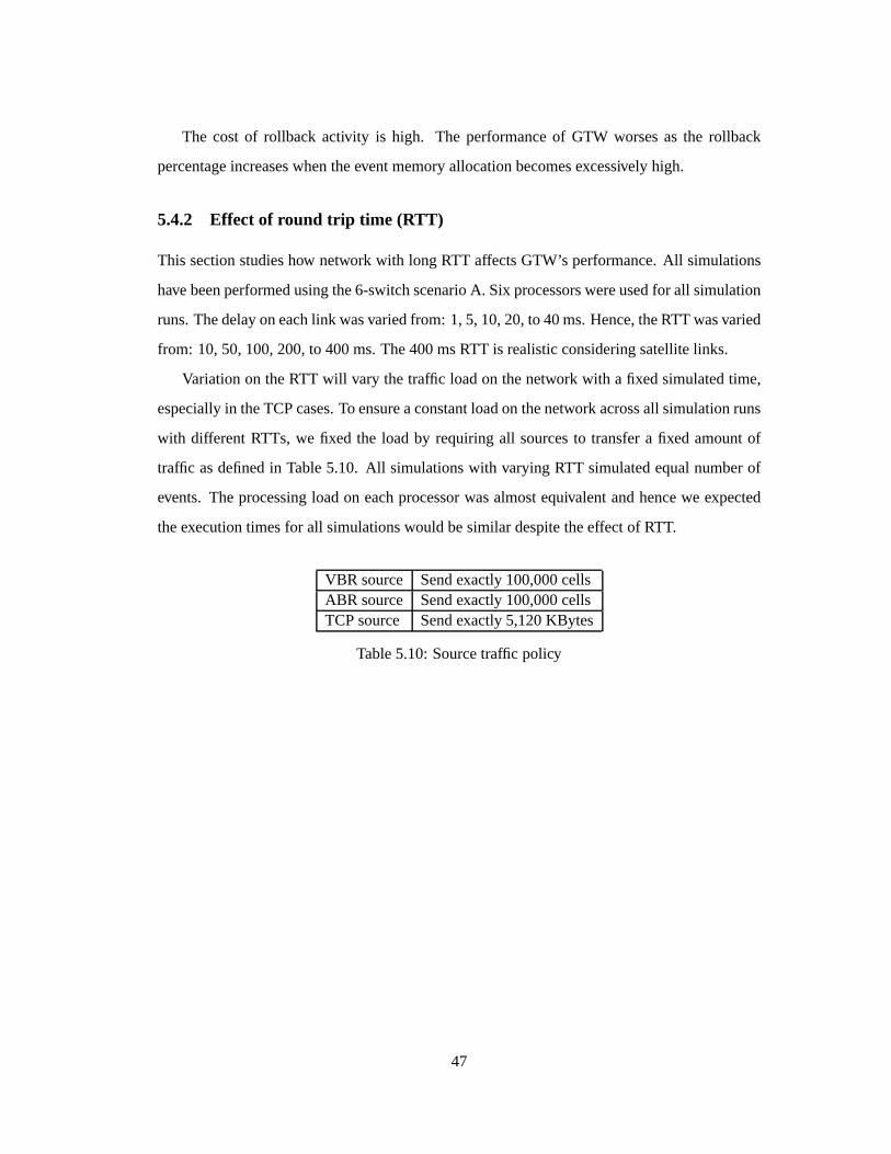
The cost of rollback activity is high. The performanceof GTW worsesas the rollback
percentageincreaseswhentheeventmemoryallocationbecomesexcessively high.
5.4.2 Effect of round trip time (RTT)
This sectionstudieshow network with long RTT affectsGTW’s performance.All simulations
havebeenperformedusingthe6-switchscenarioA. Six processorswereusedfor all simulation
runs.Thedelayoneachlink wasvariedfrom: 1,5,10,20,to 40ms.Hence,theRTT wasvaried
from: 10,50,100,200,to 400ms.The400msRTT is realisticconsideringsatellitelinks.
Variationon theRTT will vary thetraffic loadon thenetwork with a fixedsimulatedtime,
especiallyin theTCPcases.To ensureaconstantloadonthenetwork acrossall simulationruns
with differentRTTs, we fixed the load by requiringall sourcesto transfera fixed amountof
traffic asdefinedin Table5.10. All simulationswith varyingRTT simulatedequalnumberof
events. Theprocessingloadon eachprocessorwasalmostequivalentandhencewe expected
theexecutiontimesfor all simulationswouldbesimilardespitetheeffect of RTT.
VBR source Sendexactly100,000cellsABR source Sendexactly100,000cellsTCPsource Sendexactly5,120KBytes
Table5.10:Sourcetraffic policy
47
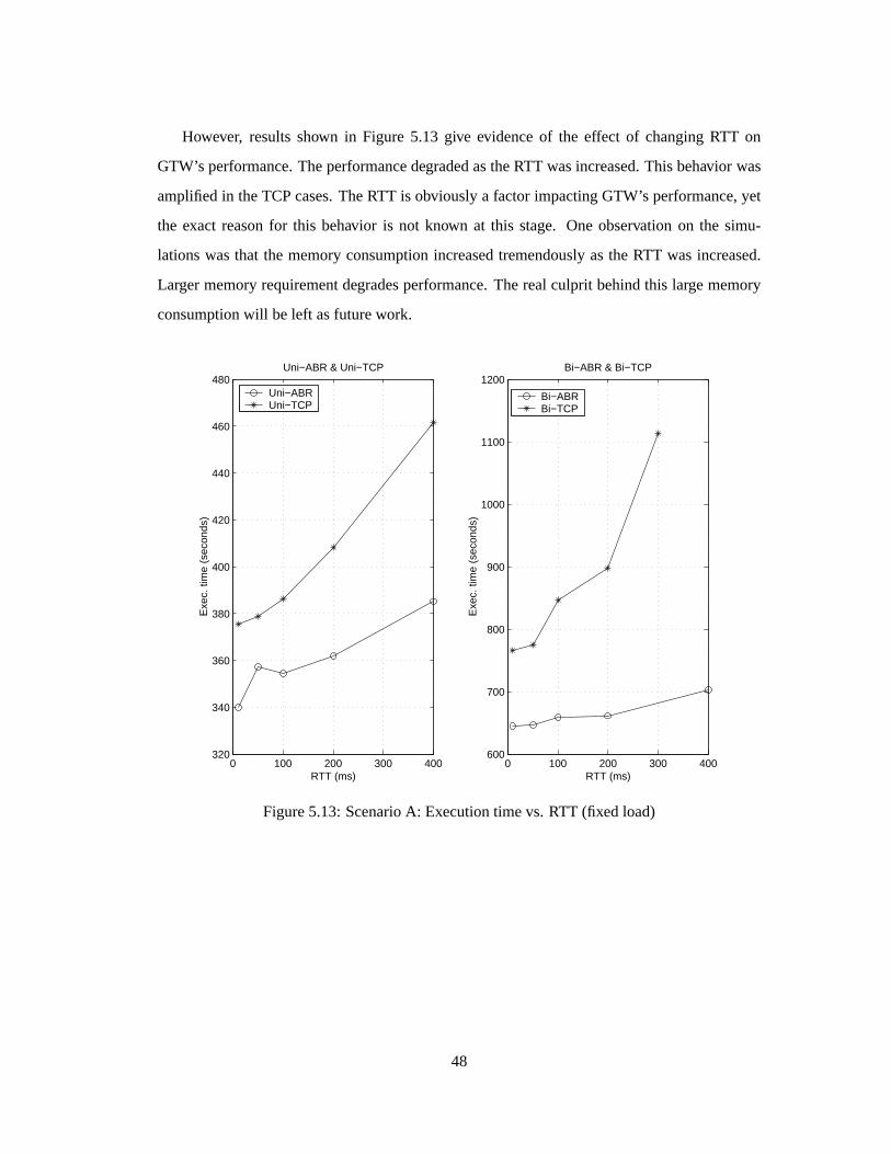
However, resultsshown in Figure 5.13 give evidenceof the effect of changingRTT on
GTW’sperformance.TheperformancedegradedastheRTT wasincreased.This behavior was
amplifiedin theTCPcases.TheRTT is obviously a factorimpactingGTW’s performance,yet
the exact reasonfor this behavior is not known at this stage. Oneobservation on the simu-
lationswasthat the memoryconsumptionincreasedtremendouslyasthe RTT wasincreased.
Largermemoryrequirementdegradesperformance.Therealculprit behindthis largememory
consumptionwill beleft asfuturework.
0 100 200 300 400320
340
360
380
400
420
440
460
480Uni−ABR & Uni−TCP
RTT (ms)
Exe
c. ti
me
(sec
onds
)
Uni−ABRUni−TCP
0 100 200 300 400600
700
800
900
1000
1100
1200Bi−ABR & Bi−TCP
RTT (ms)
Exe
c. ti
me
(sec
onds
)
Bi−ABRBi−TCP
Figure5.13:ScenarioA: Executiontimevs. RTT (fixedload)
48
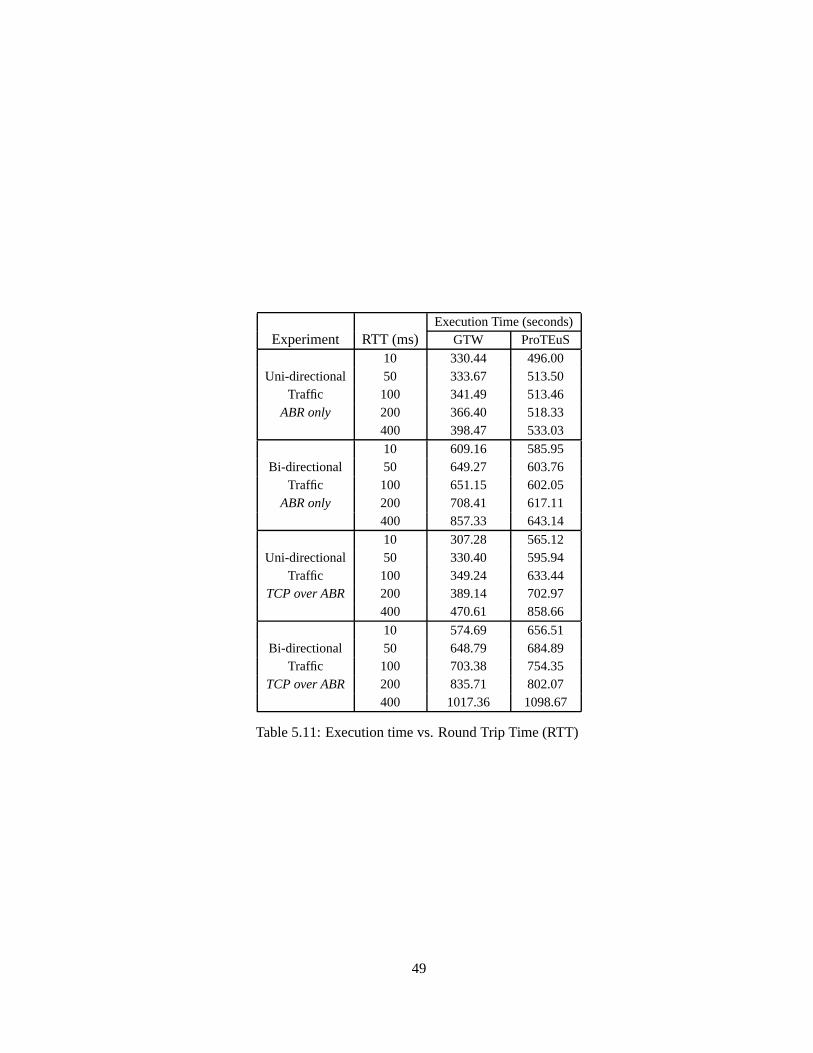
ExecutionTime(seconds)Experiment RTT (ms) GTW ProTEuS
10 330.44 496.00Uni-directional 50 333.67 513.50
Traffic 100 341.49 513.46ABRonly 200 366.40 518.33
400 398.47 533.03
10 609.16 585.95Bi-directional 50 649.27 603.76
Traffic 100 651.15 602.05ABRonly 200 708.41 617.11
400 857.33 643.14
10 307.28 565.12Uni-directional 50 330.40 595.94
Traffic 100 349.24 633.44TCPoverABR 200 389.14 702.97
400 470.61 858.66
10 574.69 656.51Bi-directional 50 648.79 684.89
Traffic 100 703.38 754.35TCPoverABR 200 835.71 802.07
400 1017.36 1098.67
Table5.11:Executiontime vs. RoundTrip Time(RTT)
49
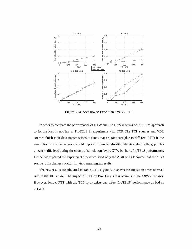
0 100 200 300 4001
1.2
1.4
1.6
1.8Uni−ABR
RTT (ms)
Nor
mal
ized
Exe
cutio
n tim
e (s
)
0 100 200 300 4001
1.2
1.4
1.6
1.8Bi−ABR
RTT (ms)
Nor
mal
ized
Exe
cutio
n tim
e (s
)0 100 200 300 400
1
1.2
1.4
1.6
1.8Uni−TCP/ABR
RTT (ms)
Nor
mal
ized
Exe
cutio
n tim
e (s
)
0 100 200 300 4001
1.2
1.4
1.6
1.8Bi−TCP/ABR
RTT (ms)N
orm
aliz
ed E
xecu
tion
time
(s)
GTW ProTEuS
Figure5.14:ScenarioA: Executiontime vs. RTT
In orderto comparetheperformanceof GTW andProTEuSin termsof RTT. Theapproach
to fix the load is not fair to ProTEuSin experimentwith TCP. The TCP sourcesand VBR
sourcesfinish their datatransmissionsat timesthatarefar apart(dueto differentRTT) in the
simulationwherethenetwork wouldexperiencelow bandwidthutilizationduringthegap.This
uneventraffic loadduringthecourseof simulationfavorsGTW but hurtsProTEuSperformance.
Hence,we repeatedtheexperimentwherewe fixedonly theABR or TCPsource,not theVBR
source.This changeshouldstill yield meaningfulresults.
Thenew resultsaretabulatedin Table5.11.Figure5.14shows theexecutiontimesnormal-
izedto the10mscase.Theimpactof RTT on ProTEuSis lessobvious in theABR-onlycases.
However, longerRTT with the TCP layer exists canaffect ProTEuS’performanceasbadas
GTW’s.
50
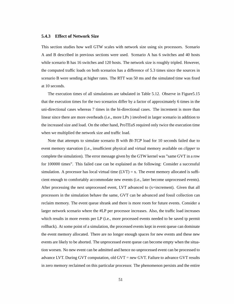
5.4.3 Effect of Network Size
This sectionstudieshow well GTW scaleswith network sizeusingsix processors.Scenario
A andB describedin previous sectionswereused. ScenarioA has6 switchesand40 hosts
while scenarioB has16switchesand120hosts.Thenetwork sizeis roughlytripled. However,
thecomputedtraffic loadson bothscenarioshasa differenceof 5.3 timessincethesourcesin
scenarioB weresendingat higherrates.TheRTT was50 msandthesimulatedtime wasfixed
at10 seconds.
Theexecutiontimesof all simulationsaretabulatedin Table5.12. Observe in Figure5.15
thattheexecutiontimesfor thetwo scenariosdiffer by a factorof approximately6 timesin the
uni-directionalcaseswhereas7 timesin the bi-directionalcases.The incrementis morethan
linearsincetherearemoreoverheads(i.e.,moreLPs) involvedin largerscenarioin additionto
theincreasedsizeandload.Ontheotherhand,ProTEuSrequiredonly twicetheexecutiontime
whenwemultiplied thenetwork sizeandtraffic load.
Note that attemptsto simulatescenarioB with Bi-TCP load for 10 secondsfailed dueto
eventmemorystarvation (i.e., insufficient physicalandvirtual memoryavailableon clipper to
completethesimulation).Theerrormessagegivenby theGTW kernelwas”sameGVT in arow
for 100000times”. This failed casecanbe explainedasthe following: Considera successful
simulation.A processorhaslocal virtual time (LVT) = x. Theeventmemoryallocatedis suffi-
cientenoughto comfortablyaccommodatenew events(i.e., laterbecomeunprocessedevents).
After processingthe next unprocessedevent, LVT advancedto (x+increment).Given that all
processorsin thesimulationbehave thesame,GVT canbeadvancedandfossil collectioncan
reclaimmemory. Theeventqueueshrankandthereis moreroomfor futureevents.Considera
largernetwork scenariowherethe#LP perprocessorincreases.Also, thetraffic loadincreases
which resultsin moreeventsperLP (i.e., moreprocessedeventsneededto besaved tp permit
rollback).At somepointof asimulation,theprocessedeventskeptin eventqueuecandominate
theeventmemoryallocated.Thereareno longerenoughspacesfor new eventsandthesenew
eventsarelikely to beaborted.Theunprocessedeventqueuecanbecomeemptywhenthesitua-
tion worsen.No new eventcanbeadmittedandhencenounprocessedeventcanbeprocessedto
advanceLVT. DuringGVT computation,old GVT = new GVT. Failureto advanceGVT results
in zeromemoryreclaimedonthisparticularprocessor. Thephenomenonpersistsandtheentire
51
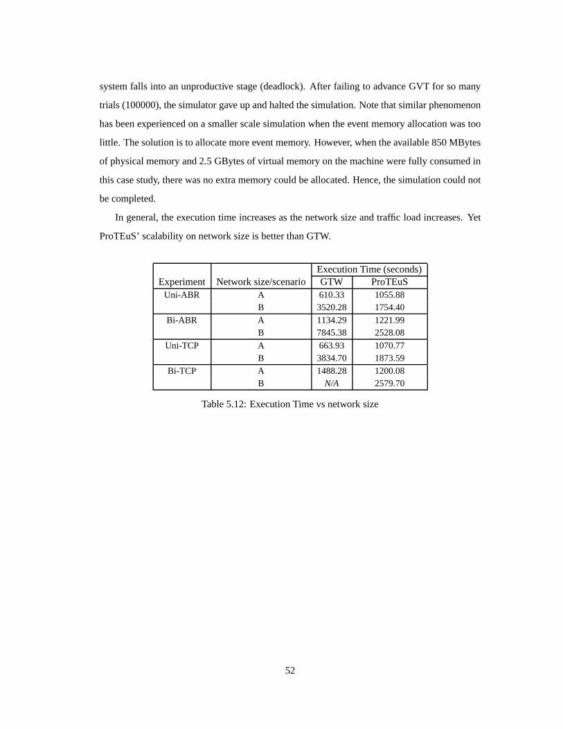
systemfalls into anunproductive stage(deadlock).After failing to advanceGVT for somany
trials (100000),thesimulatorgaveupandhaltedthesimulation.Notethatsimilarphenomenon
hasbeenexperiencedon a smallerscalesimulationwhentheeventmemoryallocationwastoo
little. Thesolutionis to allocatemoreeventmemory. However, whentheavailable850MBytes
of physicalmemoryand2.5GBytesof virtual memoryon themachinewerefully consumedin
thiscasestudy, therewasno extramemorycouldbeallocated.Hence,thesimulationcouldnot
becompleted.
In general,theexecutiontime increasesasthenetwork sizeandtraffic loadincreases.Yet
ProTEuS’scalabilityonnetwork sizeis betterthanGTW.
ExecutionTime(seconds)Experiment Network size/scenario GTW ProTEuS
Uni-ABR A 610.33 1055.88B 3520.28 1754.40
Bi-ABR A 1134.29 1221.99B 7845.38 2528.08
Uni-TCP A 663.93 1070.77B 3834.70 1873.59
Bi-TCP A 1488.28 1200.08B N/A 2579.70
Table5.12:ExecutionTimevsnetwork size
52
1 2 3 40
1
2
3
4
5
6
7Increase in execution time from scenario A to B
Uni−ABR Bi−ABR Uni−TCP Bi−TCP
Rat
io o
f exe
cutio
n tim
e −
− s
cena
rio B
/ A
GTW ProTEuS
Figure5.15:Executiontime vs. network size
53
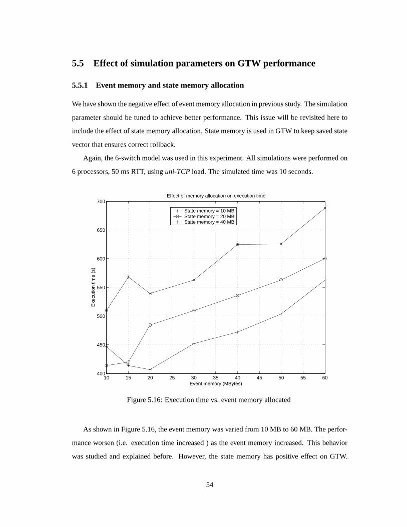
5.5 Effect of simulation parameterson GTW performance
5.5.1 Event memory and statememory allocation
Wehaveshown thenegativeeffectof eventmemoryallocationin previousstudy. Thesimulation
parametershouldbe tunedto achieve betterperformance.This issuewill be revisited hereto
includetheeffectof statememoryallocation.Statememoryis usedin GTW to keepsavedstate
vectorthatensurescorrectrollback.
Again, the6-switchmodelwasusedin thisexperiment.All simulationswereperformedon
6 processors,50 msRTT, usinguni-TCPload.Thesimulatedtime was10seconds.
10 15 20 25 30 35 40 45 50 55 60400
450
500
550
600
650
700Effect of memory allocation on execution time
Event memory (MBytes)
Exe
cutio
n tim
e (s
)
State memory = 10 MBState memory = 20 MBState memory = 40 MB
Figure5.16:Executiontimevs. eventmemoryallocated
As shown in Figure5.16,theeventmemorywasvariedfrom 10MB to 60 MB. Theperfor-
manceworsen(i.e. executiontime increased) asthe eventmemoryincreased.This behavior
was studiedand explainedbefore. However, the statememoryhaspositive effect on GTW.
54
GTW performedbetterasmorestatememorywasallocatedto the simulations. Analysison
simulationstatisticsshown that lessstatememorywould requirethe simulator to pausefor
more memoryallocationduring the courseof simulation. More pre-allocatedstatememory
preventsthisextraoverheadandthusincreasesperformance.
55
Chapter 6
Conclusionsand Futur eWork
In this thesis,theperformanceof an optimistic parallelsimulationengine,GTW, is evaluated
usinglarge-scaleATM network. Modelsof ATM switchesandend-hostshavebeenimplement-
edusingthemodelinginterface,providedby GTW, which separatestheprogrammerfrom the
simulatorkernel. Themodelingframework providesprogrammersa convenientandstructural
way to definethestateandbehavior of anobjectin sections.ThecommunicationamongLPs
aredonetrivially by sendingmessage(i.e.,eventscheduling).
As wehavedemonstrated,ATM network simulationcanbedone4 timesfasterusing6 pro-
cessorsonamultiprocessormachine.To anextent,generalnetwork simulationcantruly benefit
from time warp’s optimisticparallelsimulation.However, loadbalancingis animportantissue
to betackledbeforeanoptimumspeedupcanbeachieved. Imbalancedloadduringthecourseof
simulationoftenleadsto poorspeedupsinceidle processorswouldnotconstributeto theoverall
speedup.The currentversionof GTW requiresstaticmappingof LPs to processors.A care-
ful mappingplanmustbe doneby userto achieve goodspeedup.AutomaticLP-to-processor
mappingmechanismhasbeenproposedto makeparallelsimulatormoreuser-friendly, but such
mechanismis not yet mature. Anothermajor difficulty in performingsimulationon GTW is
that usersare requiredto tuneseveral simulationparametersin order to ensurea simulation
executessuccessfully. Severalmajorparametersrequiredto bedefinedaretheeventmemory,
statememory, local communicationpercentage,GVT period,etc. Insufficient event memory
will breakasimulationandthereis nosystematicwayto predicttheeventmemoryrequirement
(i.e.,eventmemoryrequirementdependsontheLPs’ statesizes,network characteristicssuchas
56
RTT, etc). Experienceis oftenthetool in determiningtheeventmemoryrequirement.Further
tuning,which is very time consuming,is requiredto achieve optimumperformance.Similarly,
ProTEuSneedsto addresstheissueof mappingto achieve loadbalancing.Thevalueof epoch
[17] mustbetunedto a sufficientminimumin orderto reduceexecutiontime.
In general,our evaluationhasshown thatGTW caneffectively utilize theavailableproces-
sorsto achieve greatspeedup.As the network sizegrows, moreparallelismcanbe exploited
usingmoreprocessors.However, ProTEuSoutperformedGTW in term of scalability in net-
work size.Resultsalsoshowedthatnetwork characteristicshave significantimpacton theper-
formanceof GTW. Onecharacteristicwe studiedis network with feedbackloops.We focused
on ABR serviceasits ratecontrolmechanismwith feedbacktraffic canpotentiallyinduceroll-
backs.An additionalTCPlayerontopof ABR caninducemorerollbacksandfurtherlydegrade
theperformance.Figure5.10confirmedthehypothesismade.However, thesefeedbackloops
will never impact the performanceof ProTEuSasthey do to GTW sinceProTEuSis free of
rollback. Anothernetwork characteristicwhich affectstheperformanceis theroundtrip time.
Simulationwith longerRTT requiresmoreexecutiontime. RTT haslessimpacton ProTEuS.
Interestingfuturework is discussedin below:
1. Explorenew strategiesto reducethememoryusageof theexistingmodelssincememory
consumptionlimits thesizeof network scenario.
2. Simulatearealisticscenario(i.e, takenfrom realworld carrier’sbackbone)which is often
asymmetricin topologyandloadedwith variouskindsof traffics. Studyhow well GTW
canexploit parallelismto achieve satisfactory speedupby addressingthe issueof LP-
mapping.
3. IntegrateanIP modelandvariousnetworking technologiesbesidesATM to theexisting
collectionof models.Studythefeasibility of GTW ona moregeneralnetwork.
4. ExperimentGTW on a network of workstation(NOW) platform which is moreclosely
resemblethearchitectureof ProTEuS.
57
Bibliography
[1] http://www.cadence.com.
[2] http://www.opnet.com.
[3] ATM ForumTraffic ManagementSpecificationVersion4.0. ATM ForumTechincal
Committee,Traffic ManagementSub-Working Group,April 1996.
[4] I. Akyildiz, I. Joe,R. Fujimoto,andI. Nikolaidis. ParallelSimulationof End-to-End
ATM Models.ComputerNetworksandISDNSystemsJournal, 29(6):617–630,May
1997.
[5] S.Bhatt,R. Fujimoto,A. Ogielski,andK. Perumalla.ParallelSimulationTechniquesfor
Large-ScaleNetworks. IEEE CommunicationsMagazine, pages42–47,August1998.
[6] C. CarothersandR. Fujimoto. EfficientExecutionof TimeWarpProgramson
Heterogeneous,NOW Platforms.IEEETransactionsonParallel andDistributedSystems
(pendingrevision).
[7] C. Carothers,K. Perumalla,andR. Fujimoto. EfficientOptimisticParallelSimulations
usingReverseComputation.In 1999WorkshoponParallel andDistributedSimulations,
May 1999.
[8] C. Carothers,K. Perumalla,andR. Fujimoto. TheEffectof State-saving in Optimistic
SimulationonaCache-coherentNon-uniformMemoryAccessArchitecture.In
Proceedingsof Winter SimulationConference(WSC), 1999.
[9] K. ChandyandJ.Misra. AsynchronousDistributedSimulationvia aSequenceof Parallel
Computations.Communicationsof theACM, 24(4):198– 206,April 1981.
58
[10] J.H. Cowie, D. M. Nicol, andA. T. Ogielski. Modelingtheglobalinternet.Computing
in Science& Engineering, 1(1):42–50,January/February1999.
[11] S.R. Das,R. Fujimoto,K. Panesar, D. Allision, andM. Hybinette.GTW: A Time Warp
Systemfor SharedMemoryMultiprocessors.In Proceedingsof theWinter Simulation
Conference, pages1332–1339,December1994.
[12] K. Fall. Network Emulationin theVint/NSSimulator.In ISCC99, 1999.
[13] R. Fujimoto. OptimisticApproachesto ParallelDiscreteEventSimulation.ACM
Transactionsof theSocietyfor ComputerSimulation, 7(2):91– 120,June1990.
[14] R. Fujimoto. ParallelDiscreteEventSimulation.Communicationsof theACM,
33(10):30–53,1990.
[15] R. Fujimoto,S.R. Das,andK. S.Panesar. Georgia Tech TimeWarp(GTWVersion2.3)
Programmer’s Manual. Georgia Instituteof Technology, April 1995.
[16] N. Golmie,M. Corner, Y. Saintillan,A. Koenig,andD. Su. TheNISTATM/HFCNetwork
Simulator(Version3.0)Operation andProgramming. NationalInstituteof Standards
andTechnology, March1998.
[17] S.House.ProportionalTime EmulationandSimulationof ATM Networks. Master’s
thesis,Universityof Kansas,December2000.
[18] R. Jain,S.Kalyanaraman,S.Fahmy, R. Goyal, andS.Kim. SourceBehavior for ATM
ABR Traffic Management:An Explanation.IEEE CommunicationsMagazine, 34(11):50
– 57,November1996.
[19] D. Jefferson.Virtual Time. ACM TransactionsonProgrammingLanguagesandSystems,
7(3):404–425,July 1985.
[20] W. LaRUE Jr. New Algorithmsto improvetheefficiencyof Parallel DiscreteEvent
Simulation. PhDthesis,Universityof Kansas,1996.
59
[21] S.Kalyanaraman,R. Jain,S.Fahmy, andR. Goyal. PerformanceandBuffering
Requirementsof InternetProtocolsoverATM ABR andUBR Services.IEEE
CommunicationsMagazine, 36(6):152–157,June1998.
[22] S.Kalyanaraman,R. Jain,S.Fahmy, R. Goyal, J.Jiang,andS.Kim. Performanceof TCP
overABR on ATM backboneandwith variousVBR traffic patterns.Proc. ICC’97,
Montreal, 2:1035–1041,June1997.
[23] E. Mascarenhas,F. Knop,andV. Rego. ParaSol:A MultithreadedSystemfor Parallel
Simulationbasedon Mobile Threads.In Proceedingsof the1995conferenceon Winter
simulationconference, pages690– 697,1995.
[24] R. A. Meyer. PARSECUserManual(Release1.1). UCLA ParallelComputing
Laboratory, August1998.
[25] S.Murthy. A SoftwareEmulationandEvaluationof AvailableBit RateService.Master’s
thesis,Universityof Kansas,October1998.
[26] R. PasquiniandVernonRego. OptimisticParallelSimulationover aNetwork of
Workstations.In Proceedingsof thewinter simulationconferenceonWinter simulation
(Vol. 2), pages1610– 1617,1999.
[27] K. S.Perumalla.TransparentIncrementalStateSaving in GTW++ - Design,
Implementation,VerificationandPerformanceEvaluation.Technicalreport,Georgia
Instituteof Technology, September1996.
[28] K. S.PerumallaandR. Fujimoto. GTW++ - AnObject-orientedInterfacein C++ to the
Georgia Tech TimeWarpSystem. Georgia Instituteof Technology, September1996.
[29] B. Preiss.Performanceof DiscreteEventSimulationon aMultiprocessorUsing
OptimisticandConservative Synchronization.In Proc.1990InternationalConferenceon
Parallel Processing, pages218– 222,August1990.
[30] D. StiliadisandA. Varma.A ReconfigurableHardwareApproachto Network Simulation.
ACM TransactiononModeling& ComputerSimulation, 7(1):131– 156,January1997.
60

[31] C. Williamson,B. Unger, andX. Zhonge.ParallelSimulationof ATM Networks: Case
StudyandLessonsLearned.In Proceedingsof theSecondCanadianConferenceon
BroadbandResearch (CCBR’98), pages78 – 88,June1998.
61
Recommended