American Journal of Physics and Applications 2018; 6(3): 63-75
http://www.sciencepublishinggroup.com/j/ajpa
doi: 10.11648/j.ajpa.20180603.11
ISSN: 2330-4286 (Print); ISSN: 2330-4308 (Online)
Optimization of Hydraulic Horsepower to Predict the Rate of Penetration
Herianto
Petroleum Engineering Department, Faculty of Technology and Mineral, UPN “Veteran” Yogyakarta, D. I. Yogyakarta, Indonesia
Email address:
To cite this article: Herianto. Optimization of Hydraulic Horsepower to Predict the Rate of Penetration. American Journal of Physics and Applications.
Vol. 6, No. 3, 2018, pp. 63-75. doi: 10.11648/j.ajpa.20180603.11
Received: February 22, 2018; Accepted: March 19, 2018; Published: May 10, 2018
Abstract: The rate of penetration has an important role in the success of a drilling operation, this is because if the rate of
penetration is not optimum will have an impact on the cost incurred. Some factors that influence the rate of penetration are the
weight on bit, rotation per minute and horsepower. Based on the analysis obtained WOB and RPM values are optimum so that
optimization is done on horsepower. In this case study the well that will be analyzed is vertical well so that bit’s hydraulic
optimization is performed using Bit Hydraulic Horse Power (BHHP) method by adjusting the nozzle size and circulation rate,
this method will be optimum if BHHP / HPs ratio is 65%. Evaluation on trajectory 12 ¼ well “SGT-01” field “Tranusa", obtained
bit’s hydraulics on the actual conditions at 2657.48 ft - 2723.10 ft depth interval obtained Bit Hydraulic Horse Power (BHHP) of
232.67 hp, Horse Power Surface (HPs) 499.82 hp, Horse Power per Square Inches (HSI) of 1.67 hp / in² and percentage (BHHP
/ HPs) of 46.55% (<65%) indicating less optimum then optimized hydraulic bit circulation rate optimized to 710 gpm with
Horsepower Hydraulic Horse Power (HPH) of 936.47 hp, Horse Power per Square Inches (HSI) of 5.4 hp / in² and percentage
(BHHP / HPs) of 65% (already optimum). The final result of the evaluation and optimization of bit hydraulics and the removal of
cutting is predicted to increase ROP from 46 fph to 125.66 fph.
Keywords: Hydraulic Horsepower, Drilling Optimization, ROP Prediction
1. Introduction
Increasing the complexity of drilling operations has
increased some of the issues that make drilling cost
considerations [1]. There are several parameters that affect
drilling performance and if not done properly or optimum, the
company will lose money because it does not save the cost of
drilling exactly adds to the cost issued. Some of these
parameters, among others, weight on bit (WOB), rotation per
minute (RPM), flow rate, bit hydraulics and bit type are the
most important drilling parameters affecting the rate of
penetration (ROP) and the drilling economy. The rate of
penetration is directly proportional to drilling parameters such
as WOB, RPM, and Horsepower making it a very important
methodology in considering the previous drilling data and
making optimum drill prediction [2].
It has long been known that drilling fluid properties can
dramatically impact drilling rate. This fact was established
early in the drilling literature, and confirmed by numerous
laboratory studies. Several early studies focused directly on
mud properties, clearly demonstrating the effect of kinematic
viscosity at bit conditions on drilling rate. In laboratory
conditions, penetration rates can be affected by as much as a
factor of three by aitering fluid viscosity. It can be concluded
from the early literature that drilling rate is not directly
dependent on the type or amount of solids in the fluid, but on
the impact of those solid on fluid properties, particularly on
the viscosity of the fluid as it flows through bit nozzles. This
conclusion indicates that drilling rates should be directly
correlative to fluid properties which reflect the viscosity of the
fluid at bit shear rate conditions, such as the plastic viscosity.
Secondary fluid properties reflecting solids content in the fluid
should also provide a means of correlating to rate of
penetration, as the solids will impact the viscosity of the fluid
[3].
The factors which affect rate of penetration are exceedingly
numerous and perhaps important variables exist which are
unrecognized up to this time. A rigorous analysis of drilling

64 Herianto: Optimization of Hydraulic Horsepower to Predict the Rate of Penetration
rate is complicated by difficulty of completely isolating the
variable under study. For example, interpretation of field data
may involve uncertainties due to the possibility of undetected
changes in rock properties. Studies of drilling fluid effects are
always plagued by difficulty of preparing two muds having all
properties identical except one which is under observation.
While it is generally desirable to increase penetration rate,
such gains must not be made at the expense of
overcompensating, detrimental effects. The fastest on-bottom
drilling rate does not necessarily result in the lowest cost per
foot of drilled hole. Other factors such as accelerated bit wear,
equipment failure, etc., may raise cost [4]. Optimization of
drilling hydraulics can be obtained by increasing the drilling
rate [5].
In this paper, Hydraulic horsepower has an important role in
drilling operations, the timing of drilling also greatly affects
the costs incurred. The size of the horsepower is directly
proportional to the rate of penetration (ROP) where the greater
the horsepower the faster the rate of penetration. Basically, the
parameters associated with the rate of penetration in the
drilling hydraulics include weight on bits, rotation per minute
and horsepower. Optimization of hydraulics needs to be done
to obtain optimum drilling results if the rapid penetration rate
will be obtained a good drill cleaning effect, good cutting
removal, no regrinding and no bit balling.
2. Method
The steps were taken in hydraulic optimization and cutting
removal are as follows:
1. Calculating actual bit hydraulics.
2. Calculating the actual lifting of the cutting hydraulics.
3. Calculate the maximum pressure conditions.
4. Calculating Qmin.
5. Calculating Qmax.
6. Bit hydraulics optimization.
7. Optimization of hydraulic removal of cutting.
2.1. Drilling Hydraulic and Cutting Lifting Optimization
Data processing performed on drilling hydraulics includes
calculation of pressure loss on the bit, percentage of pressure
loss on the bit and loss of surface power. Calculation of
Pressure Loss on Flow System Except on Bit (Pp) is done by
calculating the average velocity of mud and critical velocity in
both the circuit and in the annulus.
2.1.1. Calculation of Pressure Loss on Flow System Except
on Bit
Loss of pressure on the flow system except on the bit is
influenced by the flow patterns occurring within ranges and
annulus, the first step to determine the flow pattern by
calculating the average velocity of the mud and the critical
velocity of the mud, if V> Vc then the flow pattern is turbulent
otherwise V <Vc then the flow pattern is laminar (Rabia, H.,
1985).
2.1.2. Calculation of Average Flow Rate of Mud (V)
The average velocity of mud flow (V) using the equation:
QdataV
22.45 (ID )
= (1)
Where:
Q data = Data’s Rate, gpm.
ID = Inner Diameter, inch.
The average velocity of mud flow (Van) using the equation:
QdataVanDP
2 22.45 (DH - OD )
= (2)
Where:
Q data = Data’s Rate, gpm.
OD = Outer Diameter, inch.
DH = Hole Diameter, inch.
2.1.3. Critical Velocity Calculation (VC)
Critical Velocity (VC) using the equation:
�� = �.���� ��� + ���� + 12.34���������� (3)
Where:
PV = Plastic viscosity, cp.
ID = Inner Diameter, inch.
YP = Yield point, 100lb/ft.
ρm = Density, ppg.
Critical velocity in annulus (VCan) using the equation:
�� = �.����� ! � ��� + ���� + 9.256�%� − '�������� (4)
Where:
PV = Plastic viscosity, cp.
OD = Outer Diameter, inch.
DH = Hole Diameter, inch.
YP = Yield point, 100lb/ft.
ρm = Density, ppg.
After determining the flow patterns that occur in the string
and in the next annulus calculate the loss of pressure on the
surface connection (PSC). Total loss of pressure on the system
is usually expressed in the equivalent of the discharge line
consisting of 4 categories, including flow line, stand pipe,
swivel, and Kelly. Based on the type of surface connection
used in the drilling operation can be seen the price of constant
pressure loss pressure on the surface. As shown in Table 1 and
Table 2 below.

American Journal of Physics and Applications 2018; 6(3): 63-75 65
Table 1. Surface Connection Type (B. C. Craft, et. Al., 1962).
Surface eq. type
Stand pipe Rotary hose Swivel kelly
Length ID Length ID Length ID length ID
(ft) (in) (ft) (in) (ft) (in) (ft) (in)
1 40 3 40 2 4 2 40 2.25
2 40 3.5 55 2.5 5 2.5 40 3.25
3 45 4 55 3 5 2.5 40 3.25
4 45 4 55 3 6 3 40 4
Table 2. E Constanta Value Based On Surface Connection Type (B. C. Craft,
et. Al., 1962).
surface eq. type Value of E
Imperial units Metric units
1 2.5 x 10⁻⁴ 8.8 x 10⁻⁶
2 9.6 x 10⁻⁵ 3.3 x 10⁻⁶
3 5.3 x 10⁻⁵ 1.3 x 10⁻⁶
4 4.2 x 10⁻⁵ 1.4 x 10⁻⁶
The amount of pressure loss on the surface connection is
calculated by the equation:
�(� = Eρ�.�Q�.�PV�.� (5)
Where:
PSC = Pressure Loss in Surface Connection, psi. E = Surface Connection Cnstanta Type
p = Mud Density, lb/gal.
Q= Mud Rate, gpm
PV= Plastic viscosity, cp
The amount of pressure loss inside the pipe can be
calculated based on the flow pattern (B. C. Craft, et. Al.,
1962).
The flow is Laminar, then it is calculated by using the
equation:
� � ./0/�1��23²� 5.0��123² (6)
Where:
PV = Plastic viscosity, cp.
ID = Inner Diameter, inch.
L = Length, ft.
YP = Yield point, 100lb/ft.
The flow is Turbulent, then it is calculated by using the
equation:
P � 67879:7;<�1.�7=> (7)
Where:
f = friction.
ID = Inner Diameter, inch.
L = Length, ft.
V = Velocity, fps.
ρm = Density, ppg.
The value f is obtained by calculating the Reynold Number
then determined by looking at the fanning friction graph (B. C.
Craft, et. al. 1962).
Nre � B��9C>D (8)
Where:
Ρ = Fluid Density, ppg
V = Velocity, fps
d = Pipe Diameter, in
µ = effective viscosity, cp.
Figure 1. Relation of reynold number with fanning friction (Rabia, 2002)
After calculating the loss of pressure then calculates the
total pressure loss (parasitic pressure loss) on the flow system
by using the equation:
Pp = Psc + PDP + PDC + PHWDP + PMWD + PanDP + PanDC + PanHWDP + PanMWD
2.1.4. Calculation of Actual Hydraulics Bit Using BHHP
Method
The basic principle of this method assumes that the greater
the power delivered by the fluid to the rock will be the greater
the cleaning effect so that the method seeks to optimize the
horsepower used on the surface of the pump. The BHHP
concept assumes that hydraulic optimization is achieved when
the lost horsepower on the bit is 65% of its power. The BHHP
concept is suitable for drilling on vertical wells and rock types
with consideration of gravity (Rabia, H., 1985).
BHHP� E2FGF.H���I (9)
HPs� E2FGF.2FGF���I (10)
Where:
Q = Rate, gpm

66 Herianto: Optimization of Hydraulic Horsepower to Predict the Rate of Penetration
Pb = Pressure Loss on bit, psi
Calculation of how much power on the bit used to clean the
bottom of the wellbore during drilling activity, namely by
comparing BHHP price with the large power pump on the
surface (HPs) (Rabia, H., 1985).
� J%%�%�( K100%
Determining the Horse Power Per Square Inch (HSI) value:
HSI � QRRSTU7�VW�< (11)
Figure 2. Relation of ROP and Horsepower. (Carl Gatlin, 1960).
Figure 2 shows the curve relationship between horsepower
and rate of penetration. In low horsepower conditions, the
cleaning effect of small holes and small ROP. ROP price
increase can be known by increasing horsepower. But at some
point, the sharp increase in speed is achieved from the
relatively small speed (Carl Gatlin, 1960).
2.1.5. Calculation of Actual Cutting Hydraulics
Based on the physical properties of the drilling mud used,
the power law index is calculated by the equation:
2PV YPn 3.32 log
PV YP
+= + (12)
Where:
PV = Plastic Viscosity, cp.
YP = Yield point, 100lb/ft.
The Consistency Index is calculated using the equation:
( )PV YPK n511
+= (13)
Where:
PV = Plastic Viscosity, cp.
n = power law index
YP = Yield point, 100lb/ft.
Based on the mud flow rate, the diameter of the hole and the
drill pipe, the velocity of the mud flow in the annulus can be
calculated by the equation:
QVa
2 22.45 (Dh OD )=
− (14)
Where:
Q = Rate, gpm.
OD = Outer Diameter, inch.
DH = Hole Diameter, inch.
Calculate the critical velocity of mud (Vc) for power-law
fluid by equation:
1 n4 2 n 2 n3.878.(10 )K 2.4 2n 1
Vc510.ρ dh od 3n
− − + = −
(15)
Where:
K = Indeks konsistensi.
n = Indeks power law.
ρ = Density, ppg.
OD = Outer Diameter, inch.
DH = Hole Diameter, inch.
The apparent viscosity is calculated using the equation:
n1 n 12K DH OD nµan
144 Van 0.0208
− +− =
(16)
Where:
K = Consistency Index.
n = Indeks power law.
Van = Annulus Velocity, fps.
OD = Outer Diameter, inch.
DH = Hole Diameter, inch.
The vertical slip speed of cutting for the laminar flow can be
calculated using the equation:
( )282.87Ds ρs ρmVsv
µan
−= (17)

American Journal of Physics and Applications 2018; 6(3): 63-75 67
Where:
ρs = Density cutting, ppg.
Ds = cutting Diameter, inch.
ρm = mud Density, ppg.
µan = apparent Viskosity, cp.
Slip cutting speed after correction of inclination angle,
density, and RPM can be calculated using equation:
θ(600 Rpm)(3 ρm)Vs 1 Vsv
202500
− + = +
(18)
Where:
Rpm = Rotation per minute.
ρm = mud Density, ppg.
Vsv = vertical slip velocity, fps.
Cutting Transport Ratio (Ft) can be calculated using
equation:
v vα sΦτvα
−= (19)
Where:
Va = mud velocity, fps.
Vs = mud slip velocity, fps.
Cutting Concentration (Ca) can be calculated using
equation:
2(ROP) DCa 100%
14.7 Ft Q= (20)
Where:
ROP = Rate Of Penetration, ft/hr.
D = Diameter Hole, inch.
Ft = Cutting transport ratio,%.
Q = Rate, gpm.
Particle Bed Index (PBI) can be calculated by first looking
for the value of Vsa and Vsr equations:
Vsa = Vs cos Ø (21)
Vsr = Vs sin Ø (22)
Where:
Vs = slip velocity, fps.
Cutting will settle within a certain time which can be
calculated using the equation:
1(Dh - OD)
12Tsvsr
= (23)
Where:
DH = Hole Diameter, inch.
OD = Outer Diameter, inch.
Vsr = radial slip velocity, fps.
The distance taken by cutting before settling can be
calculated using the equation:
L (v v )Ta sa scDP = − (24)
Where:
Va= mud velocity, fps.
Vsa= direct mud velocity, fps.
Particle Bed Index (PBI ) can be calculated using the
equation:
1(Dh OD)(v v )a sa
12PBIL vc sr
− −= (25)
Where:
DH = Hole Diameter, inch.
OD = Outer Diameter, inch.
Va = mud Velocity, fps.
Vsa = direct mud Velocity, fps
2.2. Calculation of Pump Flow Rate and Pump Pressure
2.2.1. Calculating Qmax Pump
Calculation of the maximum pump flow rate of the
combined three pumps, namely the duplex pumps arranged in
parallel as follows:
Calculate maximum pump power (HPmax):
HPmax = HP pump max × Eff pump × Number of Pumps
Calculates maximum pump flow rate (Qmax):
Qmax = Number of Pumps × Qmax pump × Eff pump
Calculate pump maximum pressure (Pmax) using the
equation:
��XY( � �.FZ[���IEFZ[ (26)
2.2.2. Qmin with the Annular Velocity Minimum Concept
The calculation of Qmin using the Minimum Annular
Velocity method begins with determining the velocity slip
cutting (Herianto and Subiatmono, 2001). Velocity slip is the
minimum velocity where cutting can begin to rise or in
practice is a reduction in velocity mud and velocity falling
from the cutting expressed by the equation:
Vs = Vmin – Vcut (27)
Where:
Vs = slip Velocity, ft/s.
Vmin = minimum Velocity, ft/s.
Vcut = cutting Velocity, ft/s.
Vcut equation:
2
1 72
ROPVcut
dodp
dh
=
−
(28)
Where:
dodp = Pipe Outer Diameter (Dp atau Dc), in.

68 Herianto: Optimization of Hydraulic Horsepower to Predict the Rate of Penetration
dh = Borehole Diameter, in.
ROP = Rate of penetration, ft/hr.
Then corrected the Vmin Equation on all parameters
(correction of inclination, correction of density, correction to
Rpm), for vertical wells, directional, and horizontal. This
equation can be used for inclination angle 0° to 90°. The
equation is as follows:
Vmin = Vcut + Vs (29)
Where:
Vs = slip Velocity, ft/s.
Vmin = minimum Velocity, ft/s.
Vcut = cutting Velocity, ft/s.
Then the equation becomes:
min (1 * * )V Vcut C C C Vsvmwi Rpm= + + (30)
then for:
45θ ≤
(600 )(3 )min 1
202500
Rpm mV Vcut Vsv
θ ρ− + = + +
(31)
45θ ≥
(600 )(3 )min 1
4500
Rpm mV Vcut Vsv
ρ− + = + +
(32)
Where:
Vcut = cutting Velocity, ft/s.
Vsv = vertical slip Velocity ft/s.
RPM = Rotation per minute.
ρm = mud Density, ppg.
θ = incline degree (°).
Velocity cutting is a function of ROP, dodp, dh. The Vcut
equation is as follows:
2
36 1
ROPVcut
dodpCconc
dh
=
−
(33)
Where:
dodp = Pipe Outer Diameter (Dp atau Dc), in.
dh = BoreHole Diameter, in.
Cconc = cutting concentration,%.
ROP = Rate of penetration, ft/hr.
Equation of cutting concentration:
Cconc = 0.01778 ROP + 0.505 (34)
Then the mud flow rate in the annulus can be calculated by
the equation:
Qmin = K x Aannulus x Vmin
1 2 2min 3.1172 ( ) min4
Q x d d x Vh odpπ= − (35)
Where:
Qmin = minimum rate, gpm.
K = conversion constanta.
Vmin = minimum Velocity, ft/s.
dodp = Pipe Outer Diameter (Dp atau Dc), in.
dh = Borehole Diameter, in.
Calculate the total optimum nozzle area with the equation:
K � ] S:.^<��.�1�..H_
`< (36)
Where:
Q = Rate, gpm.
Pm = maximum pump pressure, psi.
Pb = pressure loss, psi.
z = power factor
Determine nozzle combination from nozzle area by
equation:
ab = �Ic d ef�g� KhijXklimmkn (37)
Where:
x = nozzle area, inch²
3. Result
WELL DATA:
Depth = 2657.48-2723.10 ft.
Hole Diameter = 12.25 in.
Diameter OD DP = 5in.
Pump rate = 660 gpm.
Plastic Viscosity = 23 cp.
Yield Point = 30 lb / 100ft.
Density mud = 11.50 ppg.
Density of drill powder = 19.39 ppg.
Diameter of drill powder = 0.16in.
The rate of penetration = 46 fph.
Inclination = 0.30°
3.1. Calculation of Actual Hydraulics
3.1.1. Calculation of Pressure Loss on Flow System Except
on Bit (Pp)
The calculation of pressure loss is done by calculating the
velocity of the mud flow in the circuit and in the annulus. An
example calculation is done on 12 ¼ trajectory Wells
"SGT-01" with Depth Interval 2657.48 ft - 2723.10 ft:
Average Velocity Calculation of Mud Flow (V)
- Velocity of average mud flow in drill pipe (VDP) using
Equation (1):
QdataVDP
22.45 (ID )=

American Journal of Physics and Applications 2018; 6(3): 63-75 69
659VDP
22.45 (4.28 )=
DP V = 14.71 fps
- Velocity of average mud flow in annulus drill pipe (Van
DP) using Equation (2):
QdataVanDP
2 22.45 (DH - OD )=
660VanDP
2 22.45 (12.25 -5 )=
VanDP = 2.15 fps
The calculation result of mud flow average in Wells
"SGT-01" in the example of Depth Interval 2657.48 ft -
2723.10 ft (trajectory 12 ¼ ") can be seen in Table 3.
Table 3. Results Calculation of Velocity of Mud Flow in Example of Depth Interval 2657.48 ft- 2723.10 ft (trajectory 12 ¼ ') Wells "SGT-01".
Mud Flow Velocity in String
Dp Dc HWDP MWD
Fps Fps fps fps
14.71 29.89 32.54 29.89
Mud Flow Velocity in Annulus
DP DC HWDP MWD
Fps fps fps Fps
2.15 3.13 2.15 3.13
Calculation of Critical Velocity (VC)
- Velocity critical on drill pipe (VCDP) with Equation
(3):
�� � 1.078���� d�� + ���� + 12.34���������g =
1.07811.50K4.28 �23 + �23� + 12.34�4.28��30K11.50� = 6.64fps
- Because VDP> VcDP then the flow that occurs is
Turbulent
- Critical Velocity in Drill pipe annulus (VCanDP) with
Equation (4):
�� = 1.078���%� − '�� d�� + ���� + 9.256�%� − '�������g =
1.07811.50�12.25 − 5� �23 + �23� + 9.256�12.25 − 5��30K11.50�= 5.60fps
Because VanDP <VcanDP then the flow is laminar
The calculation result of mud flow average in Wells
"SGT-01" in the example of Depth Interval 2657.48 ft -
2723.10 ft (12 ¼ " trajectory) can be seen in Table 4.
Table 4. Results Calculation of Critical Velocity of Mud Flow (Vc) in
Example Depth Interval 2657.48 ft - 2723.10 ft 12 ¼ " trajectory.
Critical Velocity in String
DP DC HWDP MWD
fps fps fps fps
6.64 6.88 6.91 6.88
Critical Velocity in Annulus
DP DC HWDP MWD
fps fps fps fps
5.60 5.83 5.60 5.83
Calculation of Loss of Pressure on Surface Connection (Psc).
Calculated by Equation (5), namely:
Data for surface connection:
(Table 1, for combination no 1)
Psc = t. ��.�. u�.�. ���.�
Psc =2.5K10 IK11.50�.�K659�.�K23�.�
= 391.60 psi
Calculation of Pressure Loss in Drill Pipe (PDP)
- Turbulent flow
- Calculate with Equation (8):
NreDP = 928 ���DP��DPw = 928 11.50K14.71K4.2812.79
= 47110.80
- The value of f is obtained from Figure 1 is for DP of
0.003197
- PDP Calculation with Equation (7)

70 Herianto: Optimization of Hydraulic Horsepower to Predict the Rate of Penetration
PDP = xKyDPK��K�DP��25.8����DP� = 0.003197K2570.19K11.50K14.71��25.8��4.28� = 185.38psi Calculation of Pressure Loss in Drill Pipe Annulus (PDP)
- Laminar flow
- Calculate with Equation (6):
�Xb�� = ��y���Xb��1000�%� − '����� +
��y��200�%� − '����
�Xb�� = 23K2570.19K2.151000�12.25 − 5.00�� +
30K2570.19200�12.25 − 5.00� = 55.60psi
Calculation of Total Pressure Loss in Flow System other
than the bit (Total Parasitic Pressure Loss =Pp)
Pp = Psc + PDP + PDC + PHWDP + PMWD + PanDP +
PanDC + PanHWDP + PanMWD
= 391.60 + 185.38 + 10 + 47.43 + 0.94 + 55.01 + 1.19 +
2.59 + 0.11
= 694.85 psi.
3.1.2. Calculation of Actual Hydraulics Using BHHP
Method
The percentage of pressure loss on the bit compared with
the pump pressure on the surface can be known after knowing
the magnitude of parasitic pressure loss (Pp).
Calculation of pressure loss on the bit (PB)
PB = Pdata - Pp = 1300 - 694.85 = 605.15 psi
Calculate the total optimum nozzle area with Equation (36):
ab = { Pm. Q�10.858. �}~
��
ab = { 11.5x660�10.858K605.15~
�� = 27.6in² Determine the nozzle combination of the nozzle area
obtained with Equation (37):
ab = 14 c dK32g
� K���kXℎlimmkn ⇒
27.6 = 14 K3.14K dK32g
� K4
K = 108
Calculation of BHHP data using Equation (9) and HPsdata
using Equation (10):
J%%� = u�XjX�}1714 = 660K605.151714 = 232.67hp
%�( = u�XjX��XjX1714 = 660K13001714 = 499.82hp
Calculating how much power the bit used to clean the
bottom of the wellbore during drilling, by comparing the
BHHP price with the large surface pump power (HPs).
= J%%�%�( K100% = 232.67499.82 �100% = 46.55%
Determine the price Horse Power Per Square Inch (HSI)
with Equation (11):
%�� = J%%�c4 K��ℎ��= 232.673.144 K�12.25�� = 1.97hp/in
�
3.2. Calculation of Actual Cutting Hydraulics
The calculation steps used to optimize the removal of
cutting by drilling mud using the CuttingTransport Ratio (Ft)
method, Cutting Concentration (Ca) and Particle Bed Index
(PBI) are exemplified in the calculation with Depth Interval
2657.48 ft - 2723.10 ft (trajectory 12 ¼ " ) are as follows:
Based on the physical properties of drilling mud used, the
power law index is calculated by Equation (12):
2PV YPn 3.32log
PV YP
+= +
2x23 30n 3.32log
23 30
+= +
n = 0.52
Consistency Index is calculated by using Equation (13):
( )PV YPK n511
+=
( )510 23 30K
0.51511
+=
K = 1057.464
Based on mud Rate, Hole Diameter and drill pipe, velocity
of mud flow in annulus can be calculated with Equation (14):
QVa
2 22.45 (Dh Dp )=
−

American Journal of Physics and Applications 2018; 6(3): 63-75 71
660Va
2 22.45 (12.25 5 )=
−
Va = 2.15 fps
Calculate critical mud velocity (Vc) for power law fluid
with Equation (15):
1 n4 2 n 2 n3.878.(10 )K 2.4 2n 1
Vc510.ρ dh dp 3n
− − + = −
1 0.514 2 0.47 2 0.513.878.(10 )1057.464 2.4 2x0.51 1
Vc510.x11.50 12.25 5 3x0.51
− − + = −
Vc =
377.55 fpm
Vc = 5.62 fps
Apparent Viscosity calculate with Equation (16):
n1 n 12K DH ODDp nµan
144 Van 0.0208
− +− =
0.511 0.51 121057.464 12.25 5 0.51µan
144 2.15 0.0208
− +− =
µan = 139.97 cp
Vertical cutting slip velocity for laminar flow can be
calculated with Equation (17):
( )282.87Ds ρs ρmVsv
µan
−=
( )97.139
11.5019.3920.16×82.87Vsv
−=
Vsv = 0.12 fps
Cutting slip velocity after correction of the inclination angle,
density, and RPM can be calculated using Equation (18):
θ(600 Rpm)(3 ρm)Vs 1 Vsv
202500
− + = +
0.30(600 30)(3 11.50)Vs 1 0.12
202500
− + = +
Vs = 0.12 fps
Cutting Transport Ratio (Ft ) calculated with Equation (19):
v vα sΦτvα
−=
2.15 0.121Ft
2.15
−= × 100%
Ft = 94.51%
Cutting Concentration (Ca) calculated with Equation (20):
2(ROP) D
Ca 100%14.7 Ft Q
=
659×9437.0×14.7
212.25×46Ca= x100%
Ca = 0.75%
Particle Bed Index (PBI) can be calculated by first looking
for Vsa and Vsr value using Equation (21) and Equation
(22):
- Vsa = Vs cos Ø
Vsa = 0.12 cos 0.30’
Vsa = 0.12 fps
- Vsr = Vs sin Ø
Vsr = 0.12 sin 0.30’
Vsr = 0.00063 fps
Cutting will settle within a certain time which can be
calculated using Equation (23):
1(Dh - Dp)
12Tsvsr
=
TsDP( )1 12.25 5
12
0.00063
−=
Ts = 953.02 sec.
The distance was taken by cutting before settling can be
calculated using Equation (24):
L (v v )Ta sa scDP = −
( )Lc 2.15 0.121 x953.02= −
Lc = 1934.53 ft.
Particle Bed Index (PBI ) calculated with Equation (25):
1(Dh Dp)(v v )a sa
12PBIL vc sr
− −=
( )( )112.25 5 2.15 0.121)
12PBI(1934.535) x (0.00063)
− −=
PBI = 1
The results of the actual drilling powder lift calculations
exemplified at the 2657.48 ft - 2723.10 ft (12 ¼ " trajectory)
depth can be seen in Table 5.
Table 5. Actual Cutting Lift Result on Wells "SGT-01" in Example Depth
Interval 2657.48 ft - 2723.10 ft (trajectory 12¼ ").
Depth Interval (ft) Dh === (in) Q Gpm
Drill Pipe
Ft Ca PBI
% % %
2657.48-2723.10 12.25 660 94.51 0.75 1
Furthermore, ROP, BHHP, and % BHHP / HHP are

72 Herianto: Optimization of Hydraulic Horsepower to Predict the Rate of Penetration
evaluated on the actual condition. The evaluation results of
ROP, BHHP, % BHHP / HHP at each depth interval can be
seen in Table 6.
Table 6. Evaluation Results% BHHP / HPs, ROP and BHHP Wells "SGT-01"
at Each Depth Interval (trajectory 12 ¼ ").
Depth Interval Actual
BHHP/HPs ROP BHHP
ft % ft/hr hp
909.55-1072.83 43.34 48.72 248.31
1072.83-1099.88 47.45 59.33 309.64
1099.88-1245.18 42.30 42.76 229.66
1245.18-1393.93 46.94 55.69 305.36
1393.93-1524.68 42.21 40.87 219.95
1524.68-1787.87 43.25 44.39 224.57
1787.87-1830.70 49.09 79.24 362.48
1830.70-2375.32 54.72 94.98 455.81
2375.32-2657.48 63.01 128.45 631.42
2657.48-2723.10 46.55 46 232.67
Figure 3. Graph Evaluation Depth vs ROP, BHHP and% BHHP Wells
"SGT-01" on Each Depth Interval (trajectory 12 1/4 ").
Based on the evaluation of% BHHP / HPs, ROP and BHHP
at the depth of 909.55 ft-2723.10 ft shown in Table 6 found the
price of% BHHP / Hps less optimum, where% BHHP / HPs
condition is still below 65% aims to raise the price of% BHHP
/ HPs. BHHP value is closely related to ROP value, where if
BHHP value is small then ROP is also small otherwise if
BHHP is big value then ROP is also big value, it is illustrated
in (Figure 3). Basically one of the purposes of this research is
to raise the ROP, if the ROP is high then the target drilling time
can be achieved well.
3.3. Calculation of Pump Rate and Pump Pressure
DATA:
- Pump Data
Type / Model: PZ-9 (PZ) / Duplex
Number of Units: 3
Liner Diameter: 6.5 in
Stroke Per Minute: 101.5
Qmax: 504 gpm
Hpmax / Pumps: 1000 hp
Discharge Pressure: 3400.79 psi
Efficiency: 87%
3.3.1. Calculating Qmax Pump
Calculation of the maximum pump Rate from the combined
three pumps, namely the duplex pumps arranged in parallel as
follows:
Calculate maximum pump power (HPmax):
HPmax = HP pump max × Eff pump × Number of Pumps
%��XK � 1000 × 0.87 × 3
%��XK � 2610��
Calculating the maximum pump rate (Qmax):
Qmax � NumberofPumps × Qmaxpump × Effpump Qmax � 3 × 504 × 0.87 Qmax � 1315.12���
- Calculate pump maximum pressure (Pmax) using
Equation (26):
��XK � %��XK × 1714u�XK
��XK � 2610 × 17141315.12 � 3400.79�(�
3.3.2. Calculate Qmin Pump
Qmin is calculated using the Minimum Annular Velocity
Concept in the annulus.
Calculate Cutting Concentration with Equation (34):
Cconc = 0.01778�'� � 0.505
= 0.01778�46� � 0.505
= 1.32%
Calculate cutting velocity (Vcut) with Equation (33):

American Journal of Physics and Applications 2018; 6(3): 63-75 73
Vcut � �'�36 {1 & ]'��%_
�~ ��ib�
Vcut � 4636 {1 & ] 512.25_
�~ 1.32
Vcut � 1.15fps Minimum Velocity, with Equation (31):
Vmin = Vcut + Vs Ɵ ≤ 45
Vmin � Vcut � ����600 & �����3 � ���202500 � �(�
Vmin � 1.15 � �1 �0.30�600 & 20��3 � 11.50�202500 � 0.12
Vmin � 1.27fps Minimum mud Rate in annulus with Equation (35):
Qmin � 14 c���� & i���K���bK3.1172
Qmin � 143.14�12.25� & 5��K1.27K3.1172
Qmin � 390.79gpm. The results of Minimum Annular Velocity calculations at
the "SGT-01" Wells at the 2657.48 ft - 2723.10 ft (12 × 12 cm)
Depth Interval can be seen in Table 7.
Table 7. Results of Annular Velocity Minimum Calculation at Wells "SGT-01"
in Example Interval Interval Depth 2657.48 ft - 2723.10 ft Trajectory 12¼".
Interval Cconc Vcut Vmin Qmin
ft % fps fps gpm
2657.48-2723.10 1.32 1.15 1.27 390.79
3.4. Optimization of Hydraulics and Cutting
DATA:
Depth Interval = 2657.48 ft - 2723.10 ft
Q actual = 660 gpm
P actual = 1300 psi
Pmax = 3400.79 psi
Hp pump = 1000 hp
ρm = 11.5 ppg
HD = 12.25 in
3.4.1. Hydraulic Bit Optimization
Optimization is done by trial and error by raising the Rate
parameter and pump pressure, but in trial and error also must
pay attention to the efficiency of each pump's ability to be
used optimally. On bit hydraulic optimization and removal of
"SGT-01" wells with a depth interval of 2657.48 ft-2723.10 ft.
Pumps are arranged in parallel. Results of trial and error
optimization of bit hydraulic well "SGT-01" can be seen in
Table 8.
Table 8. Results Trial and Error Optimization Hydraulics Bit at Wells
"SGT-01" in Interval example.
Depth Q Ppump BHHP HPs BHHP/HPs
(ft) gpm psi (HP) (HP) %
2657.48-2723.10 660 1300 232.39 500.58 46.42
2657.48-2723.10 670 1520 314.76 594.17 52.98
2657.48-2723.10 680 1740 399.39 690.32 57.86
2657.48-2723.10 690 1960 486.28 789.03 61.63
2657.48-2723.10 710 2260 608.81 936.17 65.03
HSI Nozzle
hp/in² 1/32in²
1.972733 27x27x277x27
2.672018 22x22x22x22
3.390471 21x21x21x21
4.128058 20x20x21x21
5.16819 19x19x20x20
After BHHP optimization, it is possible to predict the
increase of ROP by extrapolation, the result of the predicted
increase of ROP after BHHP optimization. The predicted
increase of ROP can be illustrated in (Figure 4) where the
trendline in actual condition and optimization shows the
change of ROP value after BHHP is optimized.
Extrapolation of ROP vs BHHP is obtained from the
trendline on the graph, that is:
y = 0.2149X-5.1672
y = (0.2149 x 650) -5.1672
y = 134.51 fph
Basically, in conducting an evaluation of mud hydraulics
and removal of cutting, WOB and RPM parameters are also
related to BHHP, but in this paper, the authors focus on the
evaluation and optimization of hydrolysis that is by
predicting the increase of ROP because in this case study
WOB and RPM parameters considered optimum.
At (Figure 4) it can be concluded that the predicted increase of
ROP is obtained by extrapolating linearly, so that ROP value will
be reached up to the optimum condition that is 65% BHHP / HPs,
where after passing the restriction then ROP will decrease so that
regrinding occurs (reforestation) and bit bailing.
Figure 4. Relationship of ROP vs. BHHP Wells "SGT-01" on actual
condition and optimization.
74 Herianto: Optimization of Hydraulic Horsepower to Predict the Rate of Penetration
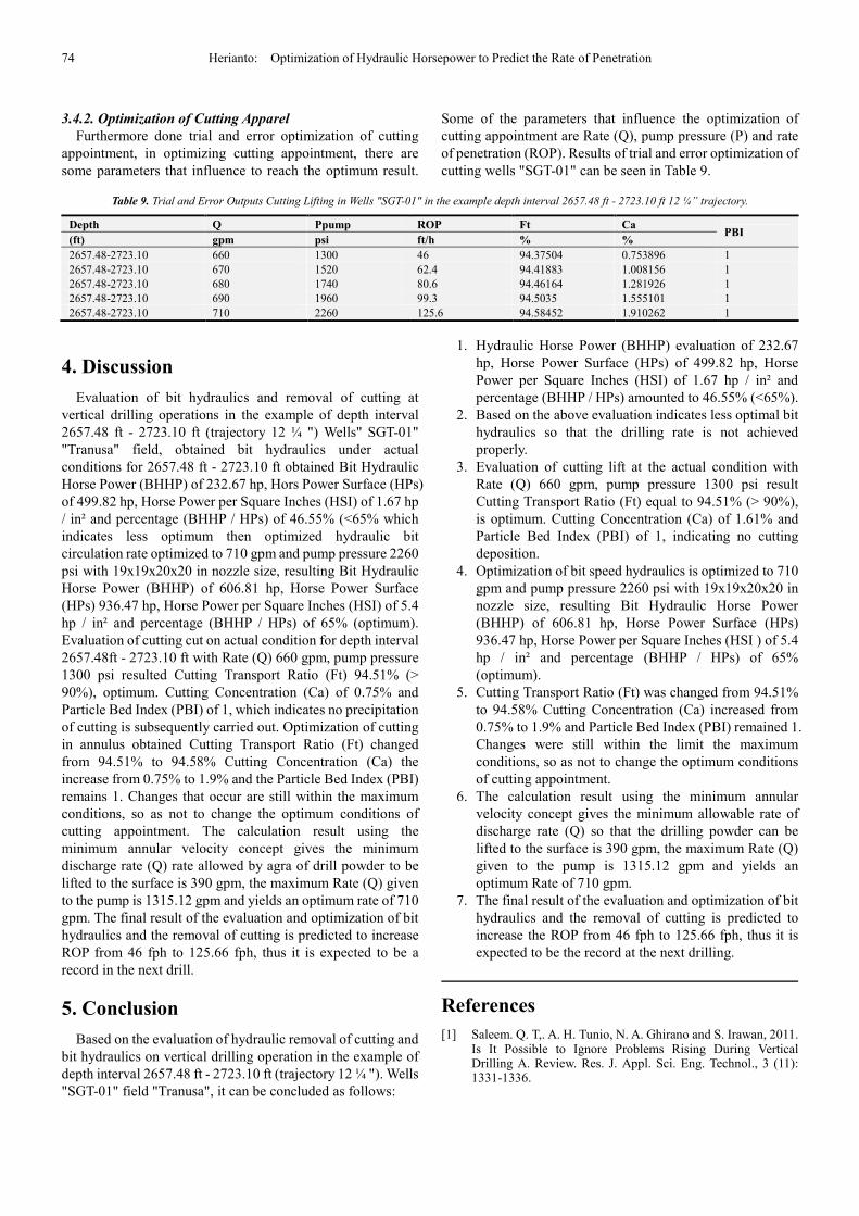
3.4.2. Optimization of Cutting Apparel
Furthermore done trial and error optimization of cutting
appointment, in optimizing cutting appointment, there are
some parameters that influence to reach the optimum result.
Some of the parameters that influence the optimization of
cutting appointment are Rate (Q), pump pressure (P) and rate
of penetration (ROP). Results of trial and error optimization of
cutting wells "SGT-01" can be seen in Table 9.
Table 9. Trial and Error Outputs Cutting Lifting in Wells "SGT-01" in the example depth interval 2657.48 ft - 2723.10 ft 12 ¼” trajectory.
Depth Q Ppump ROP Ft Ca PBI
(ft) gpm psi ft/h % %
2657.48-2723.10 660 1300 46 94.37504 0.753896 1
2657.48-2723.10 670 1520 62.4 94.41883 1.008156 1
2657.48-2723.10 680 1740 80.6 94.46164 1.281926 1
2657.48-2723.10 690 1960 99.3 94.5035 1.555101 1
2657.48-2723.10 710 2260 125.6 94.58452 1.910262 1
4. Discussion
Evaluation of bit hydraulics and removal of cutting at
vertical drilling operations in the example of depth interval
2657.48 ft - 2723.10 ft (trajectory 12 ¼ ") Wells" SGT-01"
"Tranusa" field, obtained bit hydraulics under actual
conditions for 2657.48 ft - 2723.10 ft obtained Bit Hydraulic
Horse Power (BHHP) of 232.67 hp, Hors Power Surface (HPs)
of 499.82 hp, Horse Power per Square Inches (HSI) of 1.67 hp
/ in² and percentage (BHHP / HPs) of 46.55% (<65% which
indicates less optimum then optimized hydraulic bit
circulation rate optimized to 710 gpm and pump pressure 2260
psi with 19x19x20x20 in nozzle size, resulting Bit Hydraulic
Horse Power (BHHP) of 606.81 hp, Horse Power Surface
(HPs) 936.47 hp, Horse Power per Square Inches (HSI) of 5.4
hp / in² and percentage (BHHP / HPs) of 65% (optimum).
Evaluation of cutting cut on actual condition for depth interval
2657.48ft - 2723.10 ft with Rate (Q) 660 gpm, pump pressure
1300 psi resulted Cutting Transport Ratio (Ft) 94.51% (>
90%), optimum. Cutting Concentration (Ca) of 0.75% and
Particle Bed Index (PBI) of 1, which indicates no precipitation
of cutting is subsequently carried out. Optimization of cutting
in annulus obtained Cutting Transport Ratio (Ft) changed
from 94.51% to 94.58% Cutting Concentration (Ca) the
increase from 0.75% to 1.9% and the Particle Bed Index (PBI)
remains 1. Changes that occur are still within the maximum
conditions, so as not to change the optimum conditions of
cutting appointment. The calculation result using the
minimum annular velocity concept gives the minimum
discharge rate (Q) rate allowed by agra of drill powder to be
lifted to the surface is 390 gpm, the maximum Rate (Q) given
to the pump is 1315.12 gpm and yields an optimum rate of 710
gpm. The final result of the evaluation and optimization of bit
hydraulics and the removal of cutting is predicted to increase
ROP from 46 fph to 125.66 fph, thus it is expected to be a
record in the next drill.
5. Conclusion
Based on the evaluation of hydraulic removal of cutting and
bit hydraulics on vertical drilling operation in the example of
depth interval 2657.48 ft - 2723.10 ft (trajectory 12 ¼ "). Wells
"SGT-01" field "Tranusa", it can be concluded as follows:
1. Hydraulic Horse Power (BHHP) evaluation of 232.67
hp, Horse Power Surface (HPs) of 499.82 hp, Horse
Power per Square Inches (HSI) of 1.67 hp / in² and
percentage (BHHP / HPs) amounted to 46.55% (<65%).
2. Based on the above evaluation indicates less optimal bit
hydraulics so that the drilling rate is not achieved
properly.
3. Evaluation of cutting lift at the actual condition with
Rate (Q) 660 gpm, pump pressure 1300 psi result
Cutting Transport Ratio (Ft) equal to 94.51% (> 90%),
is optimum. Cutting Concentration (Ca) of 1.61% and
Particle Bed Index (PBI) of 1, indicating no cutting
deposition.
4. Optimization of bit speed hydraulics is optimized to 710
gpm and pump pressure 2260 psi with 19x19x20x20 in
nozzle size, resulting Bit Hydraulic Horse Power
(BHHP) of 606.81 hp, Horse Power Surface (HPs)
936.47 hp, Horse Power per Square Inches (HSI ) of 5.4
hp / in² and percentage (BHHP / HPs) of 65%
(optimum).
5. Cutting Transport Ratio (Ft) was changed from 94.51%
to 94.58% Cutting Concentration (Ca) increased from
0.75% to 1.9% and Particle Bed Index (PBI) remained 1.
Changes were still within the limit the maximum
conditions, so as not to change the optimum conditions
of cutting appointment.
6. The calculation result using the minimum annular
velocity concept gives the minimum allowable rate of
discharge rate (Q) so that the drilling powder can be
lifted to the surface is 390 gpm, the maximum Rate (Q)
given to the pump is 1315.12 gpm and yields an
optimum Rate of 710 gpm.
7. The final result of the evaluation and optimization of bit
hydraulics and the removal of cutting is predicted to
increase the ROP from 46 fph to 125.66 fph, thus it is
expected to be the record at the next drilling.
References
[1] Saleem. Q. T,. A. H. Tunio, N. A. Ghirano and S. Irawan, 2011. Is It Possible to Ignore Problems Rising During Vertical Drilling A. Review. Res. J. Appl. Sci. Eng. Technol., 3 (11): 1331-1336.

American Journal of Physics and Applications 2018; 6(3): 63-75 75
[2] T. Eren and M. E. Ozbayoglu. Real time optimization of drilling parameters during drilling operations. In SPE Oil and Gas India Conference and Exhibition, 2010, SPE-129126, 2010.
[3] F. E. Beck, Arco Alaska, Inc., and J. W. Powelland MarioZamora, The Effect of Rheology on Rate of Penetration SPE/lADC Drilling Conference held In Amsterdam, 28 February-2 March 1995.
[4] A. M. Palaman, M. K. Ghassem Al-Askari, B. Salmani, B. D. Al-Anazi and M. Masihi, “Effect of Drilling Fluid Properties on Rate of Penetration”, Scientic Original Paper, 2009.
[5] Moses, A. A. and F. Engbon, 2011. Semi-analyical models on the effect of drilling fluid properties on Rate of Penetration (ROP), SPE no. 150806. Proceedings of the Nigeria Annual International Conference and Exhibition, 30 July-3, Abuja, Nigeria.
[6] Bourgoyne, A. T., et al. (1986), “Applied Drilling Engineering”, Society of Drilling Engineerings, Richardson, Texas.
[7] Gatlin, C. (1960), “Petroleum Engineering Drilling and Well Completion”, Prentice Hall Inc., Englewood Clift, New Jersey.
[8] Lummus. J. L. (1986), Drilling Fluids Optimization”, Penn Well Publishing Co., Tulsa Oklahoma.
[9] Millpark Staff (1993), “Drilling Fluid Manual”, Millaprk Drilling Fluids, A Baker Hughes Company.
[10] Preston L. Moore (1974)., “Drilling Practices Manual”, The Petroleum Publishing Co., Tulsa.
[11] Rabia, H. (1985), “Oil Well Drilling Engineering Principles and Practice”, University of New Castle, UK.
[12] Rudi Rubiandini R. S “Diklat Kuliah Teknik dan Alat Pemboran”.
[13] T. I. Larsen, A. A. Pilehvari, and J. J. Azar (1997), SPE Paper “Development of a New Cutting Transport Model for High-Angle Wellbores Including Horizontal Well”, SPE No 25872.
[14] Ziedler. H. Udo, Dr. P. E. (1988), “Drilling Fluid Technology applied to Horisontal Drilling”, Maurer Engineering Inc, Houston, Texas.
[15] Herianto. Dkk (2001) Optimisasi Hidrolika Pada Penggunaan Down Hole Mud Motor (DHMM) dengan Konsep Minimum Annular Velocity untuk Pemboran Sumur-Sumur Berarah.
[16] Norton J Lapeyrouse, “Formulas and Calculations for Drilling, Production and Workover, Second Edition”.
Recommended