1
Overview of Inferential Statistics
Jaranit Kaewkungwal, Ph.D.Faculty of Tropical Medicine
Mahidol University

2
Topics
• Bias & Chance
• Statistical Methods• Descriptive Statistics• Inferential Statistics
• Parameter Estimation• Hypothesis Testing
• Comparisons• Associations• Multi-variable Data Analysis
• Choosing the right statistical procedures

3
I
Bias & Chance

4
Bias Chance Truth
Possible Explanations of Clinical Outcomes
Bias vs.Chance
Observed = Truth + Error
Systematic error + Random error(Bias) (Chance)

5
Bias vs.ChanceObserved = Truth + Error
Systematic error + Random error
syst
olic
agegrp1 3
87
190
<=20 21−40 >= 41age group
τ
ε
τ
ε
Example of Statistical Analysis:
Analysis of variance:F = σ2
(τ+ε) /σ2ε
1890-1962
μ

6
Example of Statistical Analysis:
Regression Analysis:
Y = Y + ε
Y = α + β1 X1Cigarette Consumption per Adult per Day
12108642
CH
D M
orta
lity
per 1
0,00
0 30
20
10
0
Bias vs.ChanceObserved = Truth + Error
Systematic error + Random error
(Y = 11, X = 6)
εY=13, X = 6

7
Example of Statistical Analysis:
Chi-Square test:χ2 = Σ(Ο−Ε)2/Ε
Kappa Statistics:Observed agreement - Expected Agreement
κ = Obs Agreemt - Expct Agreemt1 - Expected Agreement
Bias vs.ChanceObserved = Truth + Error
Systematic error + Random error
100554554522No
46343YesMD#2NoYes
MD #1OBSERVED
10055455429.724.3No
4625.320.7YesMD#2
NoYes
MD #1EXPECTED

8
Bias:• A process at any stage of inference tending to produce results that depart systematically from the true values.
Bias vs.Chance
Chance:• The divergence of an observation on a sample from the true population value in either direction.• The divergence due to chance alone is called random variation
Bias and chance- are not mutually exclusive.

9
Bias vs.Chance
“A well designed, carefully executed study usually gives results that are obvious without a formal analysis and if there are substantial flaws in design or execution a formal analysis will not help.”
Johnson AF. Beneath the technological fix. J Chron Dis 1985 (38), 957-961

10
Chance
“Free kick”
Prob
abili
ty o
f bei
ng h
it
50% 50%68%95%
2.5 %2.5 %

11
Chance
“Free kick”
Prob
abili
ty o
f get
ting
goal
50% 50%68%95%
2.5 %2.5 %

12
Chance in Statistics: Descriptive Statistics
Standard Score
Raw Score
20 25 30 35 40
X = 30;SD = 5

13
Confidence Limits of μ : X + Zα/2,ν SX
X =SD = σ = 0.5 n=16
Upper LimitLower Limit
Chance in Statistics: Parameter Estimation
95% CI
μ = 80 (79.755−80.245)
μ X

14
Chance in Statistics: Hypothesis Testing
Not Reject Ho !!μ1 = μ2
Ho: μ1 = μ2Ho: μ1 − μ2 = 0Ha: μ1 − μ2 = 0
μ1 μ2

15
Chance in Statistics: Hypothesis Testing
μ1 μ2
Ho: μ1 − μ2 = 0Ha: μ1 − μ2 = 0
Reject Ho !!μ1 < μ2

16
II
Statistical Methods

17
What is Statistics?

18
Types of Statistics
• By Level of Generalization– Descriptive Statistics– Inferential Statistics
• Parameter Estimation• Hypothesis Testing
– Comparison– Association– Multivariable data analysis
• By Level of Underlying Distribution– Parametric Statistics– Non-parametric Statistics
Sampling Techniques
Generalization/Inferential Statistics
19
Descriptive Statistics

20
Descriptive Statistics
• Measure of Location (Categorical Vars)– Frequency ( f )
• Measure of Location (Continuous Vars)– Mean
– Median
– Mode
Average
Mid-point
The Most Frequent
X1 X2 X3 X4 X5 X6 X7 X8 X9
xx
n
ii
n
= =∑
1 or μ = =∑
x
N
ii
n
1
X1 X2 X3 X4 X5 X6 X7 X8 X9
( 1 2 2 2 2 3 3 4 5)
Gender
MaleFemale
Coun
t
270
260
250
240
230
220
210
Male
Female

21
Descriptive Statistics• Measure of Spread
– Range
– Standard Deviation / Variance
Max - Min
Xis deviate from Mean
xσ
μ=
−=
∑ ( )x
N
ii
n
1
Sx
n
ii
n
X=
−=
∑ ( )
- 1 1
or

22
Descriptive Statistics
• Measure of Shape– Normal Distribution
– Skewed Distribution• Positively skewed Negatively skewed

23
1. Skew = 0; “symmetric”;
median = mean
2. Skew > 0; “positive” or “right”skewed;
median<mean
3. Skew < 0; “negative” or “left”skewed;
median>mean
Descriptive Statistics

24
Example of Descriptive Statistics

25
Example of Descriptive Statistics
Mon
thly
acc
iden
tal d
eath
s (U
S)
time0 20 40 60 80
6000
8000
10000
12000
Monthly
accid
ental deaths (U
time0 20 40 60 80
6000
8000
10000
12000
Month
ly a
ccid
enta
l death
s (
U
time0 20 40 60 80
6000
8000
10000
12000
Presentation matters!
1
7
12
1 1
7 7
12
12

26
Example of Descriptive Statistics
Information can be seen in two dimensions that isn’t obvious in one dimension
Fra
ctio
n
No. of eggs10000 12000 14000
0
.05
.1
.15
Fra
ctio
n
weight4 6 8 10
0
.1
.2
.3N
o. o
f e
gg
s
weight4 6 8 10
10000
12000
14000
27
Inferential Statistics

28
Inferential Statistics
Ho: X1 = X2 Ho: μ1 = μ2
Ho: rxy = 0 Ho: ρ xy = 0
X μproportion Π
• Purpose of Inferential Statistics– Generalisabiliy of research results from Sample Statistics
to Population Parameters
• Types of Inferential Statistical Methods– Parameter Estimation - to estimate the range of values that is likely
to include the true value in population
– Hypothesis Testing - to ask whether an effect (difference) is present or not among different groups
29
Statistical Methods:Estimation

30
Parameter EstimationPoint Estimates:Single values (Mean, Variance, Correlation, treatment effect, relative risk, etc.) representing characteristics in the whole population
Interval Estimates: Ranges of values, usually centered around point estimates, indicating bounds within which we expect the true values for the whole population to lie (stability of the estimate)
Examples:• US adults have used unconventional therapy = 34%(31% - 37%, 95%CI)
•Sensitivity of clinical examination of splenomegaly =27% (19 - 36%, 95%CI)
• Relative risk of lung cancer of smoker vs. non-smoker = 5.6(2.1 - 8.9, 95%CI)
• Relative risk of HIV infected of male vs. female = 2.1 (0.5 - 6.9,95%CI)

31
Parameter EstimationApplication of Point Estimates & Confidence Intervals:
• Point estimates and confidence intervals are used to characterise the statistical precision of any rates (incidence, prevalence), comparisons of rates (e.g., relative risk), and other statistics.
• The narrower the CI, the more certain one can be about the size of the true effect. The true value is most likely to be close to the point estimate, less likely to be near the outer limits of the interval, and could (5 times out of 100) fall outside these limits altogether.
• CIs allow the reader to see the range of plausible values to decidewhether an effect size they regard as clinically meaningful is consistent with or rule out by the data.

32
Parameter Estimation
• Consideration in confidence level of the estimate
Confidence Interval, usually set at 95% CI, can be interpreted such that - if the study is unbiased and repeated 100 times, there is 95% chance that the true value is included in these intervals
Select a cut-point for CI

33
Example of
Estimate&
95%CI

34
Example of
Estimate&
95%CI

35
Statistical Methods:Hypothesis Testing
• Comparison among different groups
• Association among variables
• Multi-variable Data Analysis (MDA)(Statistical Modeling)

36
Statistical Methods:Hypothesis Testing - Comparisons

37
Hypothesis Testing Comparison of Qualitative Outcome Variable
Total Sample (N)
No exposure Group (N2)
Exposure Group (N1)
No Outcome
(n12)
No Outcome
(n22)
Outcome (n11)
Outcome (n21)

38
·
Outcome No Outcome
Exposure
No Exposure
Hypothesis Testing Comparison of Qualitative Outcome Variable
(n11) (n12)
(n21) (n22)
(N1)
(N2)
(N)
Cross-sectional

39
·
Outcome No Outcome
Exposure
No Exposure
Hypothesis Testing Comparison of Qualitative Outcome Variable
(n11) (n12)
(n21) (n22)
(N1)
(N2)
(N)
Cohort

40
·
Outcome No Outcome
Exposure
No Exposure
Hypothesis Testing Comparison of Qualitative Outcome Variable
(n11) (n12)
(n21) (n22)
(N1)
(N2)
(N)
Case-Control
41
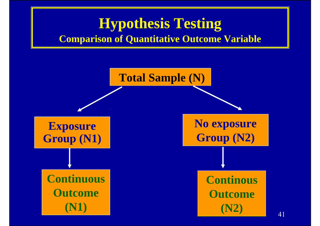
Hypothesis Testing Comparison of Quantitative Outcome Variable
Total Sample (N)
No exposure Group (N2)
Exposure Group (N1)
Continuous Outcome
(N1)
ContinousOutcome
(N2)

42
Hypothesis Testing Comparison of Quantitative Variable (Outcome)
•• Scatter Plot of the dataScatter Plot of the data
• Do you observe a similar amount of variation within each sample?• What about the weight gains? Is there any evident difference?

43
Hypothesis Testing Comparison of Quantitative Variable (Outcome)
••SideSide--byby--side Box plotsside Box plots
• The dots represent the sample average in each group of observations.• Does this graph show any difference among the groups?

44
Hypothesis Testing Comparison of Quantitative Variable (Outcome)
••SideSide--byby--side Box plotsside Box plots
The large variation within groups in the top figure suggests that the difference among the sample medians could be simply due to chance variability.
The data in the picture below are much more convincing that the populations differ.
( )21 −=
xxt
S12/n1 + S2
2/n2

45
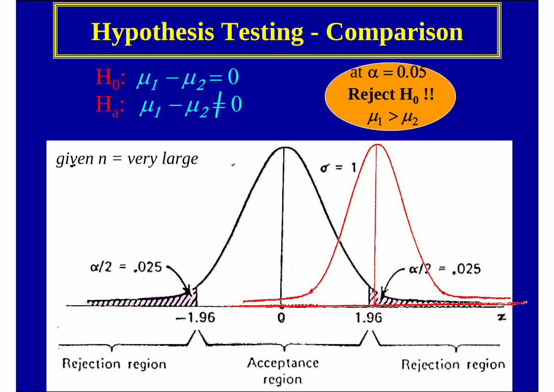
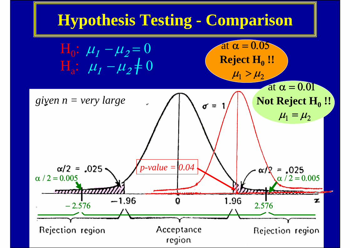
Hypothesis Testing - Comparison
• Basic steps in hypothesis testing
46
Hypothesis Testing - Comparisonat α = 0.05Reject H0 !!
μ1 > μ2
H0: μ1 − μ2 = 0 Ha: μ1 − μ2 = 0
given n = very large

47
Hypothesis Testing - Comparison
• Considerations in hypothesis testing1. What is your outcome of interest?2. What/who are the comparison groups?4. What is/are the hypothesis/hypotheses to be
tested?3. What is a cut-point for decision making about
the hypothesis/hypotheses?

48
Hypothesis Testing - Comparison
• Hypothesis & Tail of the test– One-sided vs. Two-sided Test
Two-sided test:Ex Ho: Outcome 1 = Outcome 2
Ha: Outcome 1 ≠ Outcome 2One-sided test:
Ex Ho: Outcome 1 ≤ Outcome 2Ha: Outcome 1 > Outcome 2Ho: Outcome 1 ≥ Outcome 2Ha: Outcome 1 < Outcome 2
O1<O2 | O1=O2 | O1>O22.5% 95% 2.5%
O1<O2 | O1 >= O25% 95%

49
Hypothesis Testing - Comparison
• Cut-point for decision making (p-value)The p-value is a quantitative estimate of the probability that observed differences in treatment effects in the particular study at hand could have happened by chance alone, assuming that there is in fact no difference between the groups.Or,If there is no difference between treatments and the trial was repeated many times, what proportion of the trials would lead to the conclusion that a treatment is as or more effective than found in the study?
Customary convention: p-value is set at 0.05• < 1 chance in 20 is a small risk of being wrong in decision making process• At the rate of 1/20, it is reasonable to conclude that such an occurrence is unlikely to arisen by chance alone
• Some researchers prefer to report the exact probabilities (e.g., 0.03, 0.001,0.11), rather than lumping them into two categories, p < 0.05 or p > 0.05.
50
Hypothesis Testing - Comparisonat α = 0.05Reject H0 !!
μ1 > μ2
H0: μ1 − μ2 = 0 Ha: μ1 − μ2 = 0
α / 2 = 0.005
− 2.576
α / 2 = 0.005
2.576
at α = 0.01Not Reject H0 !!
μ1 = μ2
given n = very large
p-value = 0.04

51
Exa
mpl
e of
Com
pari
sons

52
Example ofComparisons

53
Preliminary Results of the Phase III Efficacy Trial of AIDSVAX B/B February 23, 2003
All Volunteers 98/1679 (5.8%) 191/3330 (5.7%) 3.8% (-22.9 to 24.7%)
White & Hispanic 81/1508 (5.4%) 179/3003 (6.0%) -9.7% (-42.8 to 15.7%)
Black/Asian/Other 17/171 (9.9%) 12/327 (3.7%) 66.8% (30.2 to 84.2%)*66.8% (30.2 to 84.2%)*
Black 9/111 (8.1%) 4/203 (2.0%) 78.3% (29.0 to 93.3%)**78.3% (29.0 to 93.3%)**
Asian 2/20 (10.0%) 2/53 (3.8%) 68.0% (-129.4 to 95.5%)
Other 6/40 (15.0%) 6/71 (8.5%) 46.2% (-67.8 to 82.8%)
Vaccine EfficacyWeighted cohort Placebo Inf./total Vaccine Inf./total VE (95.12%CI)
** p <0.02* p <0.01
Example of Comparisons

54
Example ofComparisons
∗∗∗

55
Statistical Methods:Hypothesis Testing - Associations

56
Associations
Statistics are also used to describe the degree of association between variables.• Pearson’s product moment correlation for interval data• Spearman’s rank correlation for ordinal data• Odds Ratio , Relative Risk for ordinal or nominal data • etc.
These statistics expressed in quantitative terms the extent to which the value of one variable is associated with the value of the other.
The association coefficient has a corresponding statistical test to assess whether the observed association is greater than might have arisen by chance alone.

57
AssociationsQuantitative Variables
Thig
h c
ircum
fere
nce (
cm
Knee circumference (cm)30 35 40 45 50
40
60
80
100
Many interesting features can be seen in a scatterplot including the overall pattern (i.e. linear, nonlinear, periodic), strength and direction of the relationship, and outliers (values which are far from the bulk of the data).

58
Associations Quantitative Variables
y
x-2 -1 0 1 2
-2
-1
0
1
2
y
x-2 -1 0 1 2
-2
-1
0
1
2
y
x-2 -1 0 1 2
0
1
2
3
4
Perfect positive correlation
(R = 1)
Perfect negative correlation
(R = -1)
Uncorrelated (R = 0)
but dependent

59
Associations Quantitative Variables
y
x0 2 4 6
.4
.6
.8
1
1.2
Scatterplot showing nonlinear relationship
s1
s30 20 40 60
0
20
40
60
O
Scatterplot showing daily rainfall amount (mm) at nearby stations in SW Australia.
Note outliers -- Are they data errors … or interesting science?!

60
Scatterplot of bodyfat vs. height (inches)
HEIGHT
80706050403020
BO
DY
FAT
40
30
20
10
0
Associations Quantitative Variables

61
Scatterplot of bodyfat vs. height (inches)
HEIGHT
787674727068666462
BO
DY
FAT
40
30
20
10
0
Associations Quantitative Variables
62
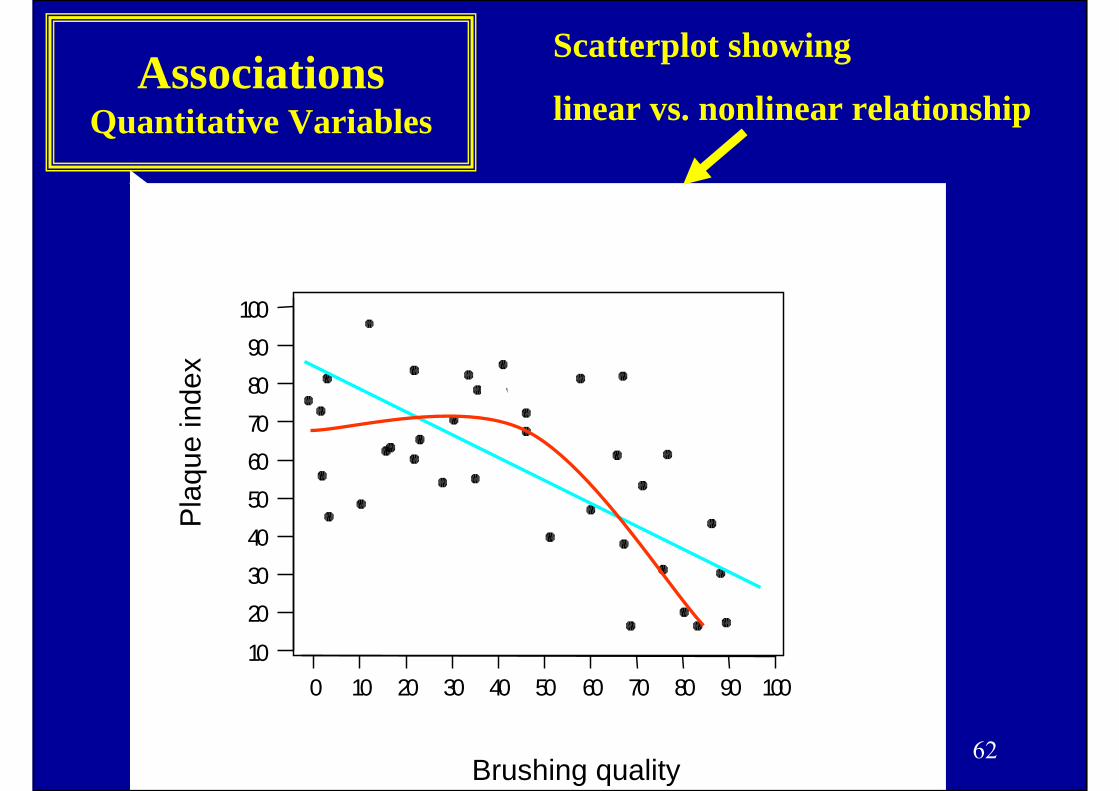
Associations Quantitative Variables
1009080706050403020100
1009080706050403020
10
Pla
que
inde
x
Brushing quality
Scatterplot showing
linear vs. nonlinear relationship

63
Associations Quantitative Variables
Scatterplot showing
linear vs. nonlinear relationship
1009080706050403020100
100908070605040302010
Pla
que
inde
x
Brushing quality
{ { { {{1 2 3 4 5

64
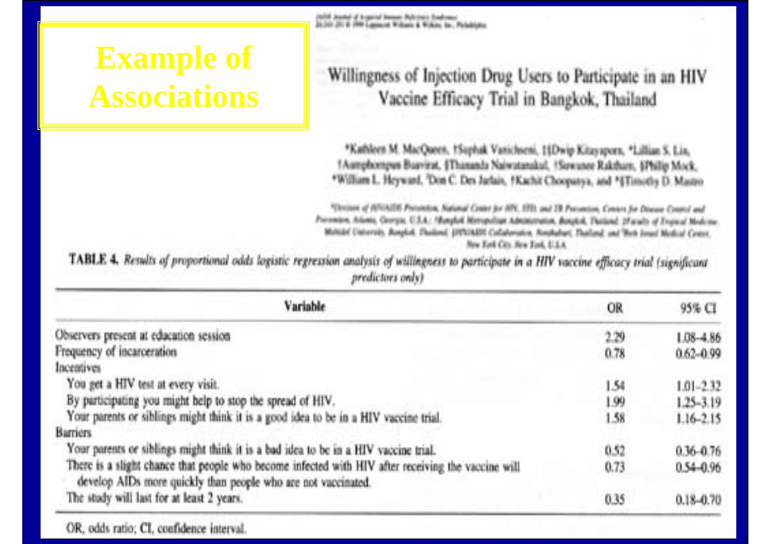
Example ofAssociations

65
Example ofAssociations

66
Associations Qualitative Variables
To assess whether two factors are related, construct an R x C table that cross-classifies the observations according to the two factors.
Example. Education versus willingness to participate in a study of a vaccine to prevent HIV infection if the study was to start tomorrow. Counts, percents and row and column totals are given.
d e f i n i t e l yn o t
p r o b a b l yn o t
P r o b a b l y d e f i n i t e l y T o t a l
< h i g hs c h o o l
5 21 .1 %
7 91 .6 %
3 4 27 .0 %
2 2 64 .6 %
6 9 9
h i g h s c h o o l 6 21 .3 %
1 5 33 .2 %
4 1 78 .6 %
2 6 25 .4 %
8 9 4
s o m ec o l l e g e
5 31 .1 %
2 1 34 .4 %
6 2 91 3 .0 %
3 7 57 .7 %
1 2 7 0
c o l l e g e 5 41 .1 %
2 3 14 .8 %
5 7 11 1 .8 %
2 4 45 .0 %
1 1 0 0
s o m e p o s tc o l l e g e
1 80 .4 %
4 60 .9 %
1 3 92 .9 %
7 41 .5 %
2 7 7
g r a d u a t e /p r o f
2 50 .5 %
1 3 92 .9 %
3 3 06 .8 %
1 1 62 .4 %
6 1 0
T o t a l 2 6 4 8 6 1 2 4 2 8 1 2 9 7 4 8 5 0
The table displays the joint distribution of education and willingness to participate.

67
Associations Qualitative Variables
The marginal distributions of a two-way table are simply the distributions of each measure summed over the other.
E.g. Willingness to participateDefinitelynot
Probablynot
Probably Definitely
264 861 2428 12975.4% 17.8% 50.1% 26.7%
A conditional distribution is the distribution of one measure conditional on (given the) value of the other measure.
E.g. Willingness to participate among those with a college education.
Definitelynot
Probablynot
Probably Definitely
54 231 571 2444.9% 21.0% 51.9% 22.2%
68
Example of Associations

69
Example of Associations
Odds = P (disease) / P (no disease)= (disease/total) / (no disease/total)
Odds Ratio = Odds Grp1 / Odds Grp2
Odds (<=18,500 cpm) = 7.5|92.5 = .08Odds (> 18,500 cpm) = 29.6|70.4 = .42Odds Ratio = .42/.08 = 5.25
(8/107) / (99/107)

70
Example of
Associations
71
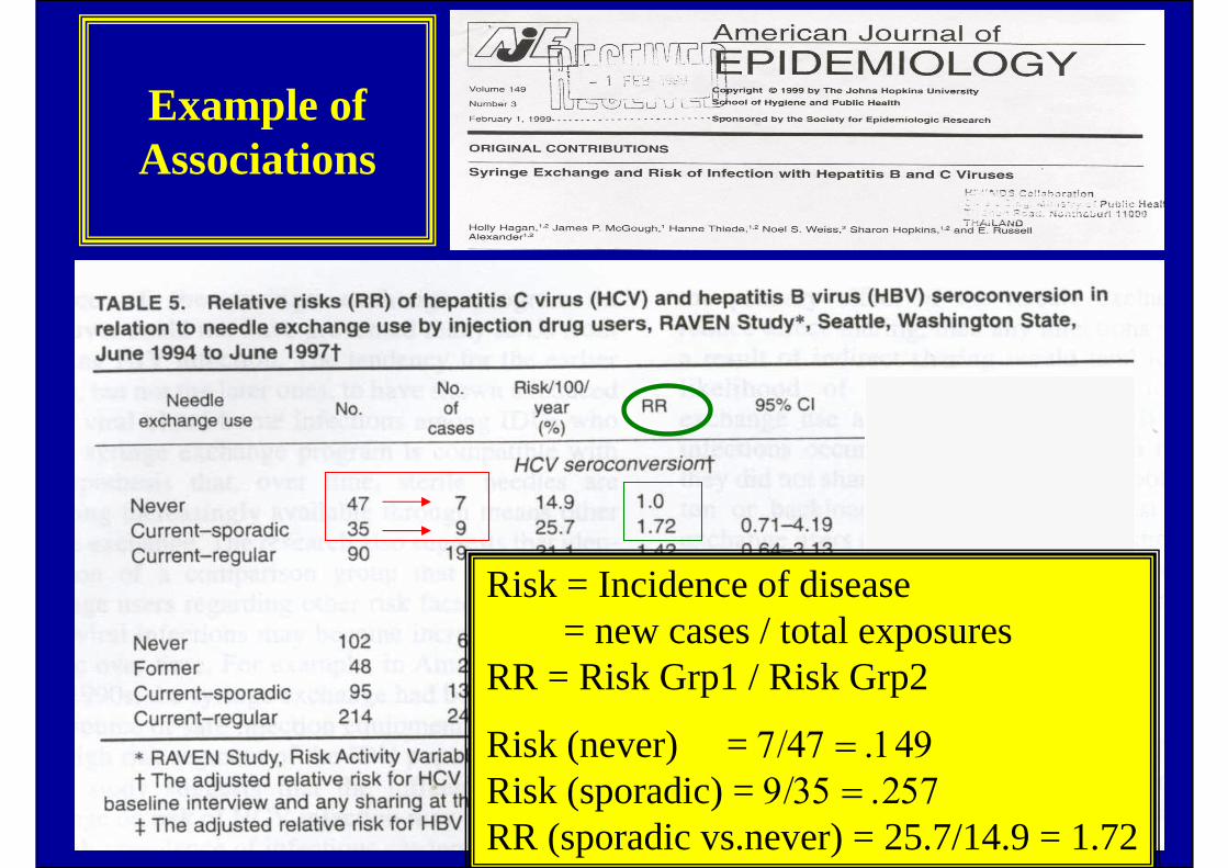
Example of Associations
Risk = Incidence of disease= new cases / total exposures
RR = Risk Grp1 / Risk Grp2
Risk (never) = 7/47 = .149Risk (sporadic) = 9/35 = .257RR (sporadic vs.never) = 25.7/14.9 = 1.72

72
Example of Associations

73
Statistical Methods:Multi-variable Data Analysis

74
Multi-variable Data Analysis Types of Epidemiological/Clinical Studies
75
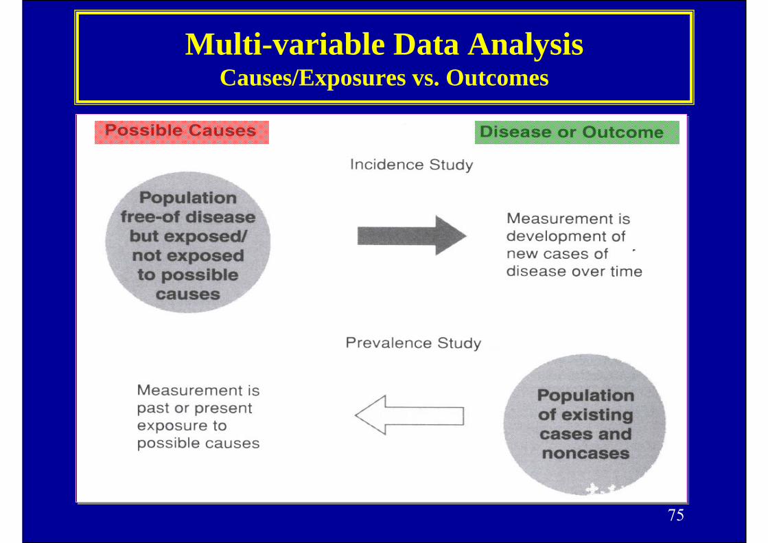
Multi-variable Data Analysis Causes/Exposures vs. Outcomes
76
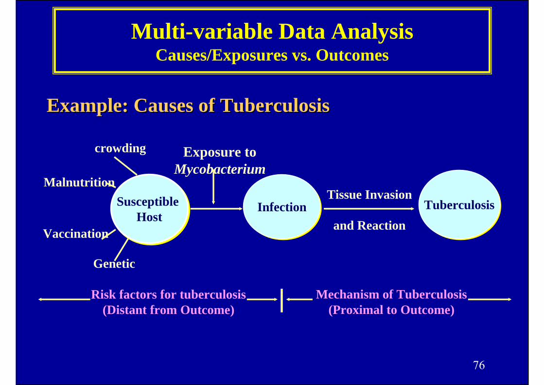
Multi-variable Data Analysis Causes/Exposures vs. Outcomes
crowding
Malnutrition
Vaccination
Genetic
Risk factors for tuberculosis(Distant from Outcome)
Mechanism of Tuberculosis(Proximal to Outcome)
Susceptible Host
Susceptible Host
InfectionInfection TuberculosisTuberculosisTissue Invasion
and Reaction
Exposure to Mycobacterium
ExampleExample:: Causes of TuberculosisCauses of Tuberculosis

77
Multi-variable Data Analysis Causes/Exposures vs. Outcomes
Example: Relationship between risk factors and disease : hypertension ( BP) and congestive heart failure (CHF). Hypertension causes many diseases, including congestive heart failure, and congestive heart failure has many causes, including hypertension.
78
Multi-variable Data AnalysisStatistical Modelling
Most clinical outcomes are the result of many variables acting together in complex ways.
Basic steps in performing MDA:• First try to understand the relationships by examining relatively simple arrangement of the data (e.g., 2 x 2 table), examining whether the effect of one variable is changed by the presence or absence of one or more other variables (stratified analysis).
• In addition to contingency tables, examine the effects of several variables simultaneously at one time using “multi-variable modelling” methods.

79
Multi-variable Data AnalysisStatistical Modelling
• Considerations in MDA• What are the right variables to be included in the model?• What are the right amount of variables to be included in the model?• What is the best model to explain the phenomenon?

80
Multi-variable Data AnalysisStatistical Modelling
• the right variables to be included in the model• identify and measure all the variables that might
be related to the outcome of interest• What is the definition of each variable?• How do you make decision in classifying your subjects?
• the right amount of variables• reduce the number of variables to be considered in the model to manageable number, usually no more than several.
• Often this is done by selecting variables that are, when taken one at a time, most strongly related to the outcome. • Evidence for the biological importance of the variable is alsoconsidered in making the selection.

81
Multi-variable Data AnalysisStatistical Modelling
• the “best” model• try different models and select the theoretical model that is best fitted to the data
• Statistical model may vary from one data-set to another. The validity of the model is based on the assumptions about the data that may not be met or it is sensitive to random variation. • The model is thus needed to be validated. This is commonly done by seeing if the model predicts what is found in another independent sample of patients. The results of the first model are considered a hypothesis, to be tested by new data.

82
Exampleof
MDA
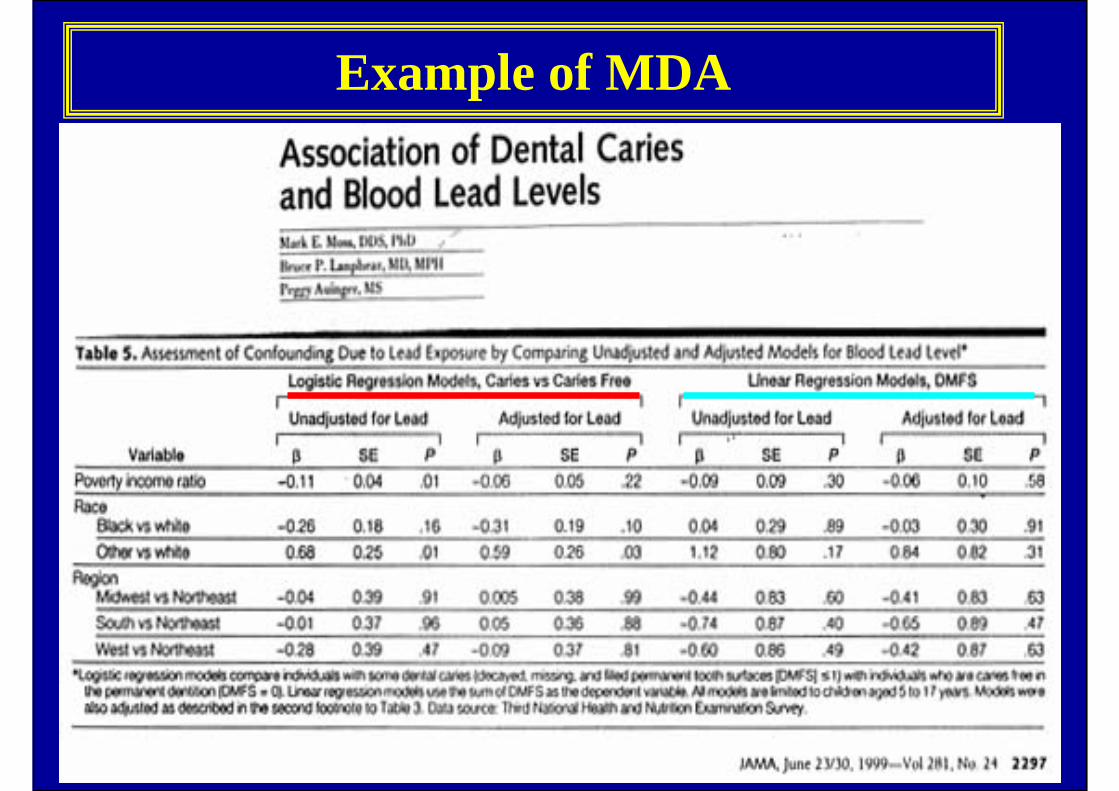
83
Example of MDA

84
Exampleof
MDA

85
Example of MDA

86
Example of MDA

87
IIIChoosing the Right Statistical Procedure

88
Choosing the Right Data Analysis Procedure
Basic questions that you should have answers before you can choose the correct test are the following:
What is the purpose of the analysis?- describe the data; Or- compare groups of data to make decisions; or- examine the association between variables for
prediction or forecasting?
Is the distribution of the data approximately normal?
Is the sample size large enough that the Central Limit Theoremwill allow a normality assumption?

89
Selecting a Statistical Method
Goal Type of Outcome Dataof the Continuous Categorical Binomial Survivalanalysis (from Gaussian Continuous Time
Population) (Non-Gaussian)
DescribeValue of Data
(1 Group)
CompareValue of Data
vs. Hypothetical
Value(1 Group)
Mean,SD
Median,Interquar-tile range
Proportion(Percent)
Kaplan-Meier survival curve
One-sample t-test
Wilcoxon’s test
Chi-square (χ2) orBinomial/ Runs test

90
Selecting a Statistical Method
Goal Type of Outcome Dataof the Continuous Categorical Binomial Survivalanalysis (from Gaussian Continuous Time
Population) (Non-Gaussian)
CompareValues 2 Grpsof Indept >2 GrpsGrps.
CompareValues 2 Grpsof Paired >2 GrpsGrps/Vars.
Unpaired t-test
One-way ANOVA
Mann-Whitney test
Kruskal-Wallis test
χ2 test , Fisher’s Exact,
χ2 test
Log-rank / Mantel-HaenszelCox Prop Haz.Reg.
Paired t-test
Repeated measures ANOVA
Wilcoxon’s test
Friedman’s test
McNemar’s χ2
test
Cochrane’s Q test
Condtn Prop Haz.Reg.
Condtn Prop Haz.Reg.

91
Selecting a Statistical Method
Goal Type of Outcome Dataof the Continuous Categorical Binomial Survivalanalysis (from Gaussian Continuous Time
Population) (Non-Gaussian)
Quantify Association
Values of Two variables(1 Group)
Predict Value of Outcome Var:from 1 Var
(Simple Reg. )from > 2 Vars(Multiple Reg.)
Pearson’s Correlation
Spearman’s Correlation
Contingency coefficient, Crude Odds Ratio, Relatv Risk
Linear orNon-linear
Regression.
Cox’s Proportional Haz. Reg.
Non-parametricRegression
Logistic Regression

92
Selecting a Statistical Method
Goal Type of Outcome Dataof the Continuous Categorical Binomial Survivalanalysis (from Gaussian Continuous Time
Population) (Non-Gaussian)
Measures of Agreement Values
from Two Raters/Methods
Measures of Validity
Values from Two Raters/Methods
Pearson’s Correlation
Weighted Kappa (κ)
Weighted Kappa (κ)
Agreement rate
Cohen’s κ
ICC
ANOVA
Factor Analysis
Non-parametric ANOVA
Factor Analysis
χ2
SensitivitySpecificityROC curve

93
Example: Selecting a Statistical Method

94
Exa
mpl
e: S
elec
ting
a St
atis
tical
Met
hod
r = 0.31
r = 0.05

95
Exa
mpl
e: S
elec
ting
a St
atis
tical
Met
hod

96
Example: Selecting a Statistical Method
Dose-Response

97
Example: Selecting a Statistical Method
Charactersitcs No. of No. of Patients 7-Year survival, Rate ratio patients who died % % (95% CI)* (95% CI)** Age at Infection, years <= 19 105 31 (29.5) 72.3 (62.1-80.1) Referent >=20 89 35 (39.3) 63.3 (50.5-73.6) 1.50 (0.92-2.45) Sex work Brothel 159 54 (34.0) 69.6 (61.1-76.6) 1.34 (0.71-2.52) Nonbrothel 35 12 (34.3) 62.9 (41.6-78.2) Referent Oral contraceptive use Yes 112 36 (32.1) 69.6 (59.2-77.9) 0.83 (0.51-1.36) No 82 30 (36.6) 67.1 (54.7-76.8) Referent Depot medroxyprogesterone use Yes 55 18 (32.7) 70.9 (55.7-81.7) 0.78 (0.45-1.37) No 139 48 (34.5) 67.8 (58.4-75.5) Referent Infection status Seroconverted 34 7 (20.6) *** 1.42 (0.63-3.22) Seropositive at enrl. 160 59 (36.9) 69.6 (61.4-76.4) Referent Viral load, HIV-1 RNA copies/ml. >1000,000 34 24 (70.6) 34.5 (18.8-50.9) 15.40 (5.2-45.2) 10,000-100,000 113 38 (33.6) 70.3 (60.1-78.4) 4.63 (1.64-13.1) <10,000 47 4 (8.5) 92.5 (78.4 -97.5) Referent Total 194 66 (34.0) 68.7 (61.0-75.2) * Survival analysis ** Cox proportional hazard model *** Insufficient follow-up time to this m ore recent converted group; 5-year survival = 77.8 (56.8-89.5) %
Table 2. Survival from time of infection of 194 HIV-infected CSWs

98
Example: Selecting a Statistical MethodSu
rviv
al (%
)
Months
10 20 30 40 50 60 70 80 90 100 110 1200
20
40
60
80
100
A B
Months
10 20 30 40 50 60 70 80 90 100 110 120
20
40
60
80
100 <10,000
>100,000
10,000-100,000
00 0
Surv
ival
(%)
Figure 2. Survival from time of human immunodeficiency virus (HIV) infection of 194 CSWs.
A, Overall. B, By serum virus load (HIV type 1 RNA copies/mL).
Each curve is truncated when <10 women remain in that group.

99
Example: Selecting a Statistical Method
Charactersitcs No. of No. of Pts 5-Year survival, Rate ratio Adjusted rate ratiopatients who died % % (95% CI)* (95% CI)** (95% CI)***
Initial CD4 lymphocyte, cells/μL<200 15 14 (93.3) 0 20.9 (9.00-48.7) 15.5 (6.46-37.4)200-500 88 34 (38.6) 63.4 (51.8-72.9) 2.46 (1.21-5.01) 1.42 (0.67-3.00)>500 54 10 (18.5) 84.7 (70.4-92.4) Referent Referent
Viral load, HIV-1 RNA copies/ml.>1000,000 30 23 (76.7) 26.7 (12.6-43.0) 13.9 (4.78-40.6) 12.5 (4.09-38.2)10,000-100,000 89 31 (34.8) 65.0 (53.1-74.5) 3.87 (1.36-11.0) 3.42 (1.19-9.81)<10,000 38 4 (10.5) 96.7 (78.6-99.5) Referent Referent
Total 157 58 (36.9) 64.6 (56.0-71.9)
* Survival analysis** Cox proportional hazard model*** Cox proporational hazard model adjusted for initial CD4 lymphocyte count and virus load
Table 3. Mortality from time of first CD4 T lymphocyte count of 157 HIV-infected CSWs (125 women were HIV seropositive at study enrollment and 32 seroconvertedduring study).
Recommended