Performance evaluation of Performance evaluation of parallel programsparallel programs
Moreno MarzollaDip. di Informatica—Scienza e Ingegneria (DISI)Università di Bologna
Pacheco, Section 2.6
Performance Evaluation 2

Performance Evaluation 3
Credits
● prof. David Padua– https://courses.engr.illinois.edu/cs420/fa2012/lectures.html
Performance Evaluation 4
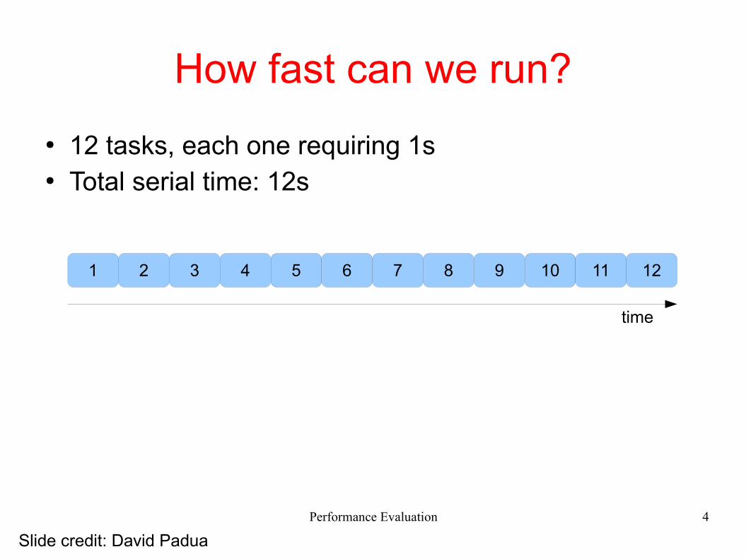
How fast can we run?
● 12 tasks, each one requiring 1s● Total serial time: 12s
1 2 3 4 5 6 7 8 9 10 11 12
time
Slide credit: David Padua
Performance Evaluation 5
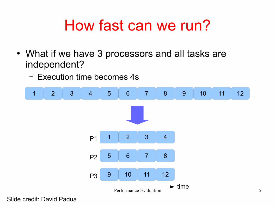
How fast can we run?
● What if we have 3 processors and all tasks are independent?– Execution time becomes 4s
1 2 3 4 5 6 7 8 9 10 11 12
1 2 3 4
5 6 7 8
9 10 11 12
P1
P2
P3
Slide credit: David Padua
time
Performance Evaluation 6
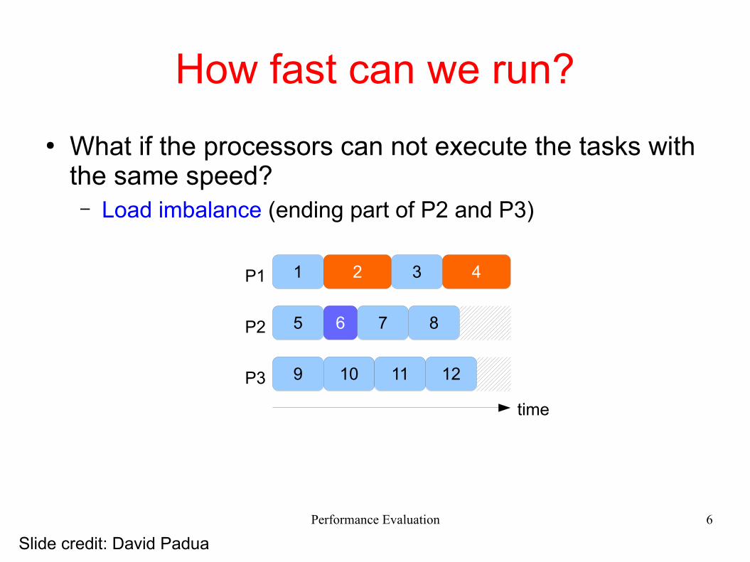
How fast can we run?
● What if the processors can not execute the tasks with the same speed?– Load imbalance (ending part of P2 and P3)
1 2 3 4
5 6 7 8
9 10 11 12
P1
P2
P3
Slide credit: David Padua
time
Performance Evaluation 7
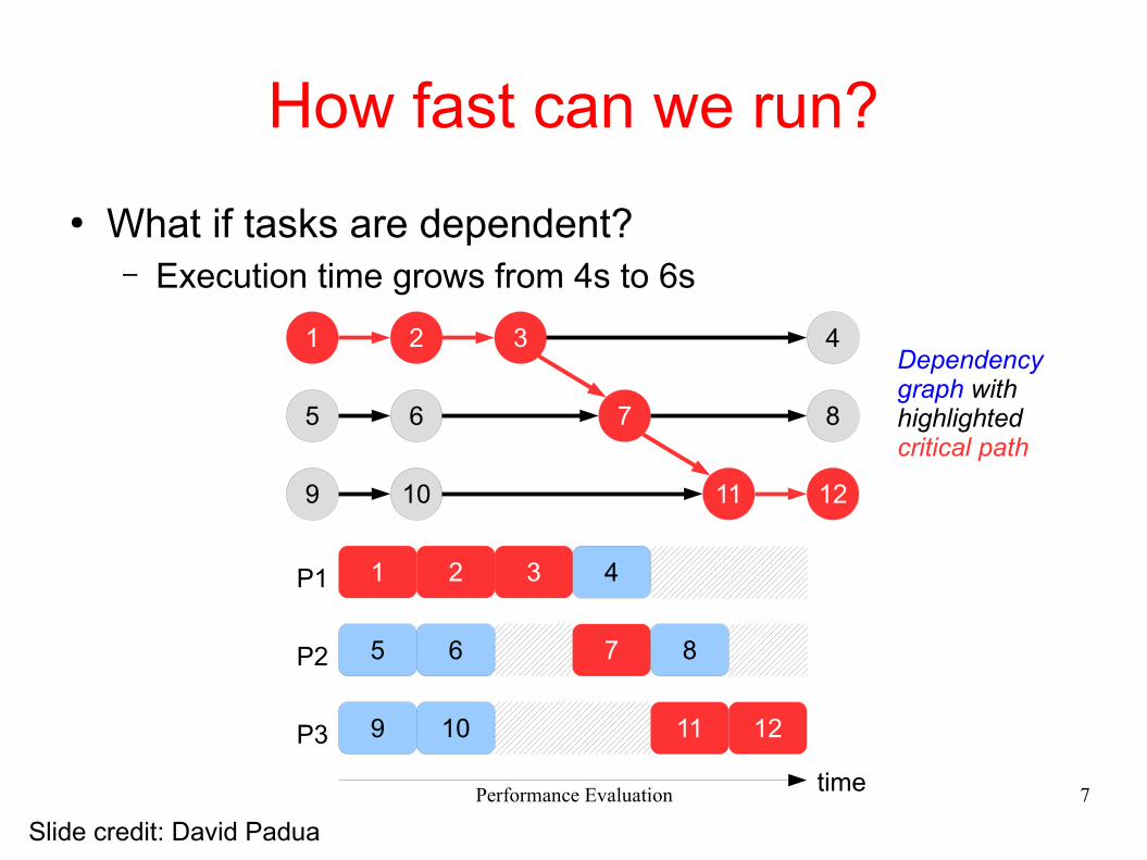
How fast can we run?
● What if tasks are dependent?– Execution time grows from 4s to 6s
1 2 3 4
5 6 7 8
9 10 11 12
P1
P2
P3
1 2 3
5 6 7
9 10 11
4
8
12
Dependency graph with highlighted critical path
Slide credit: David Padua
time
Performance Evaluation 8
Scalability
● How much faster can a given problem be solved with p workers instead of one?
● How much more work can be done with p workers instead of one?
● What impact for the communication requirements of the parallel application have on performance?
● What fraction of the resources is actually used productively for solving the problem?
Slide credit: David Padua
Performance Evaluation 9
Speedup ● Let us define:
– p = Number of processors / cores– Tserial = Execution time of the serial program
– Tparallel (p) = Execution time of the parallel program with p processors / cores
Performance Evaluation 10
Speedup
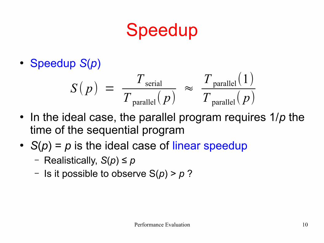
● Speedup S(p)
● In the ideal case, the parallel program requires 1/p the time of the sequential program
● S(p) = p is the ideal case of linear speedup– Realistically, S(p) ≤ p– Is it possible to observe S(p) > p ?
S ( p) =T serial
T parallel( p)≈T parallel(1)
T parallel( p)
Performance Evaluation 11
Warning
● Never use a serial program to compute Tserial
– If you do that, you might see a spurious superlinear speedup that is not there
● Always use the parallel program with p = 1 processors
Performance Evaluation 12
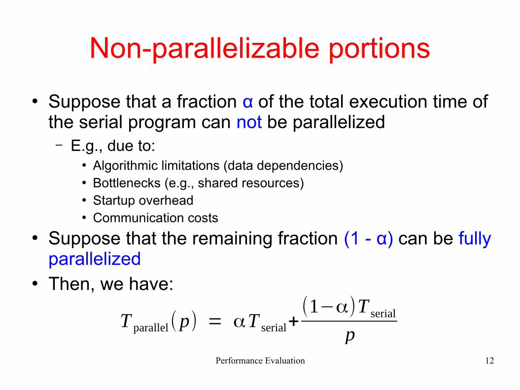
Non-parallelizable portions
● Suppose that a fraction α of the total execution time of the serial program can not be parallelized– E.g., due to:
● Algorithmic limitations (data dependencies)● Bottlenecks (e.g., shared resources)● Startup overhead● Communication costs
● Suppose that the remaining fraction (1 - α) can be fully parallelized
● Then, we have:
T parallel(p) = αT serial+(1−α)T serial
p
Performance Evaluation 13
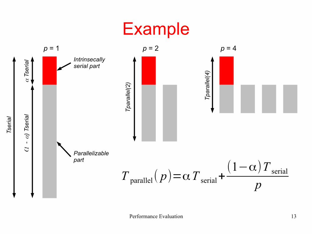
Example
Intrinsecally serial part
Parallelizable part
p = 1 p = 2 p = 4
Tser
ial
α T
seri
al
(1 - α
) Ts
eri
al
T parallel( p)=αT serial+(1−α)T serial
p
Tp
ara
llel(
2)
Tp
ara
llel(
4)
Performance Evaluation 14
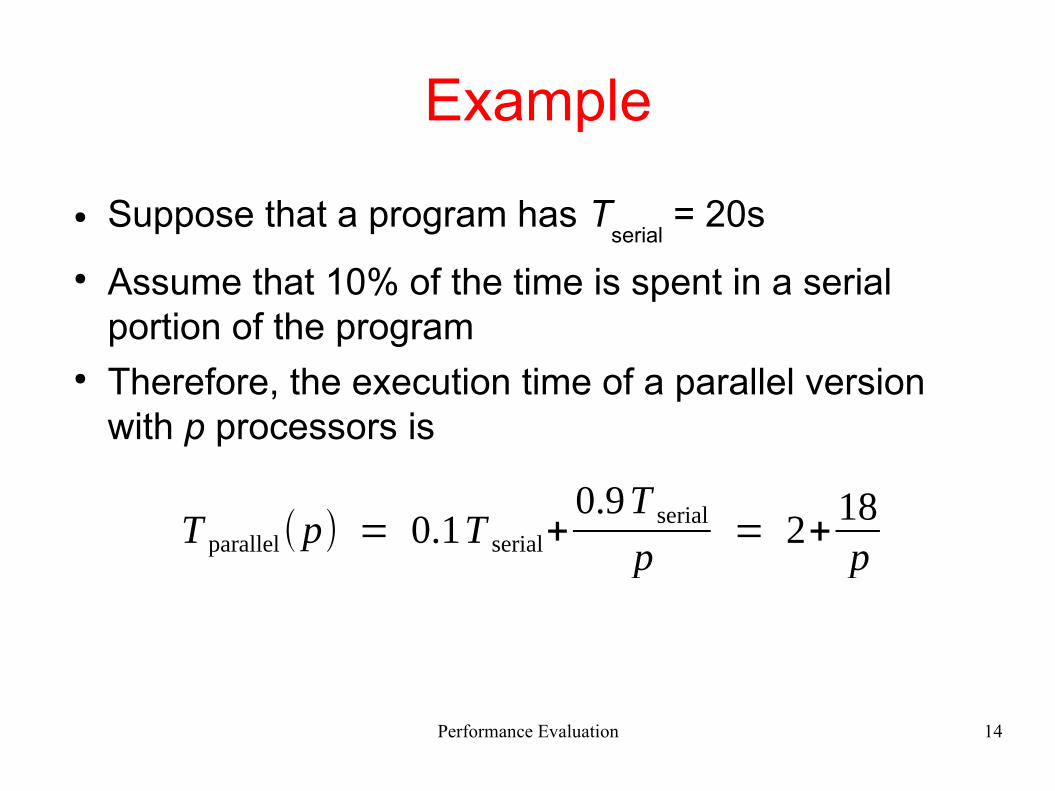
Example
● Suppose that a program has Tserial
= 20s
● Assume that 10% of the time is spent in a serial portion of the program
● Therefore, the execution time of a parallel version with p processors is
T parallel(p) = 0.1T serial+0.9T serialp
= 2+18p
Performance Evaluation 15
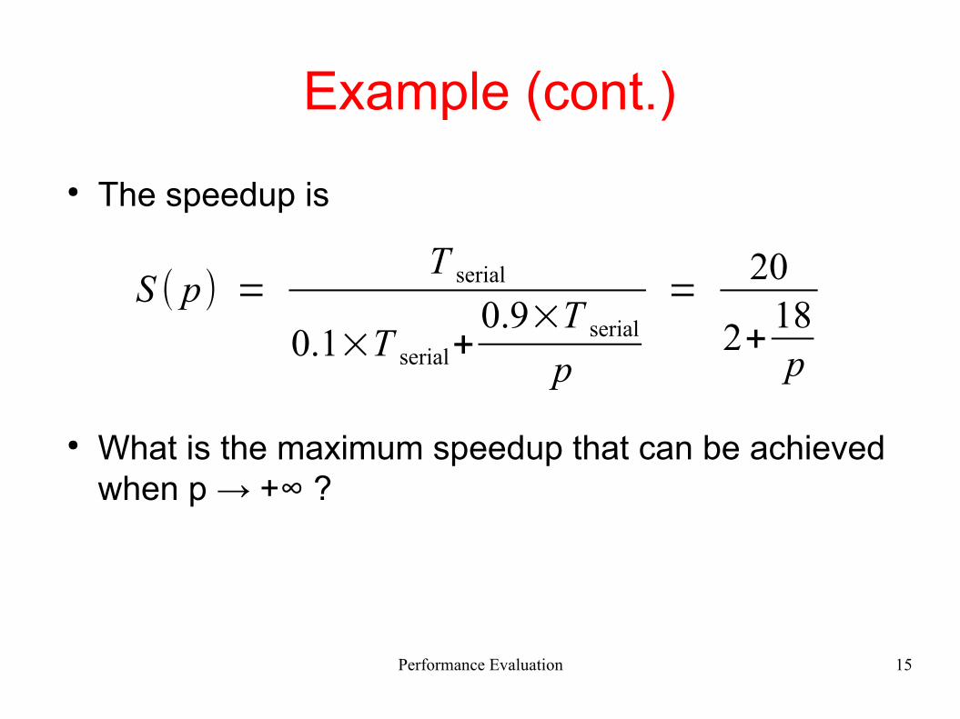
Example (cont.)
● The speedup is
● What is the maximum speedup that can be achieved when p → +∞ ?
S ( p) =T serial
0.1×T serial+0.9×T serial
p
=20
2+18p
Performance Evaluation 16
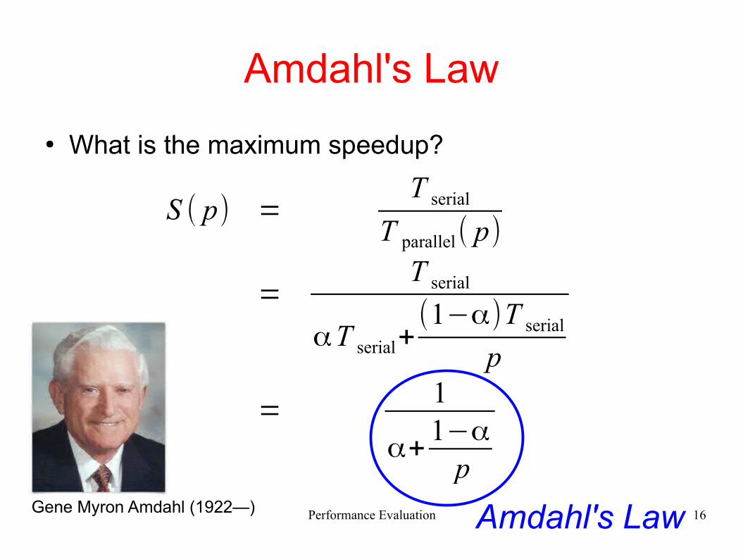
S ( p) =T serial
T parallel( p)
=T serial
αT serial+(1−α)T serial
p
=1
α+1−α
p
Amdahl's Law
● What is the maximum speedup?
Gene Myron Amdahl (1922—) Amdahl's Law
Performance Evaluation 17
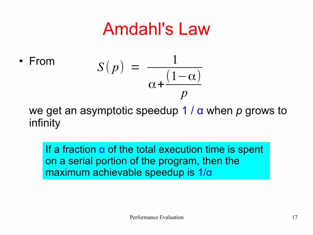
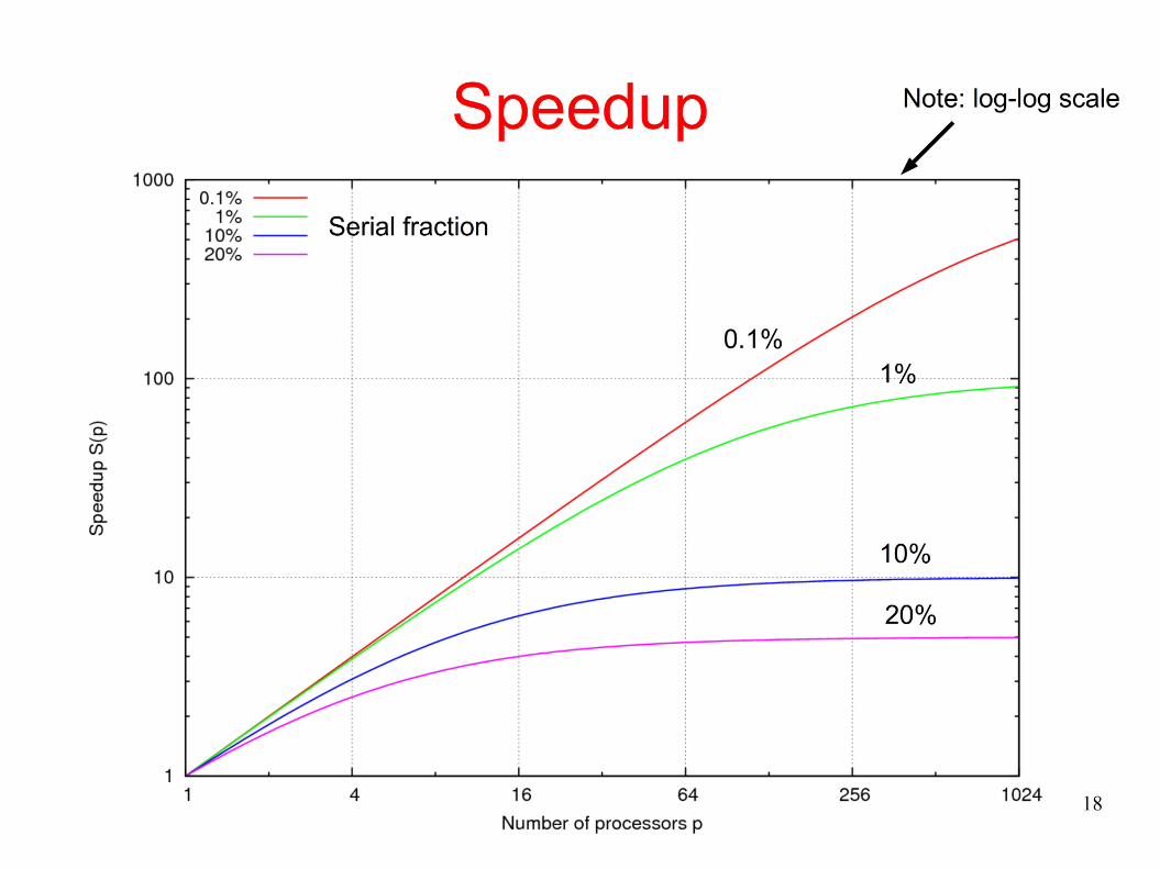
Amdahl's Law
● From
we get an asymptotic speedup 1 / α when p grows to infinity
S ( p) =1
α+(1−α)
p
If a fraction α of the total execution time is spent on a serial portion of the program, then the maximum achievable speedup is 1/α
Performance Evaluation 19
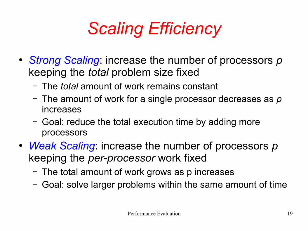
Scaling Efficiency
● Strong Scaling: increase the number of processors p keeping the total problem size fixed– The total amount of work remains constant– The amount of work for a single processor decreases as p
increases– Goal: reduce the total execution time by adding more
processors● Weak Scaling: increase the number of processors p
keeping the per-processor work fixed– The total amount of work grows as p increases– Goal: solve larger problems within the same amount of time
Performance Evaluation 20
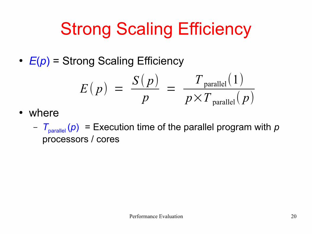
Strong Scaling Efficiency
● E(p) = Strong Scaling Efficiency
● where– Tparallel (p) = Execution time of the parallel program with p
processors / cores
E ( p) =S ( p)p
=T parallel(1)
p×T parallel( p)
21
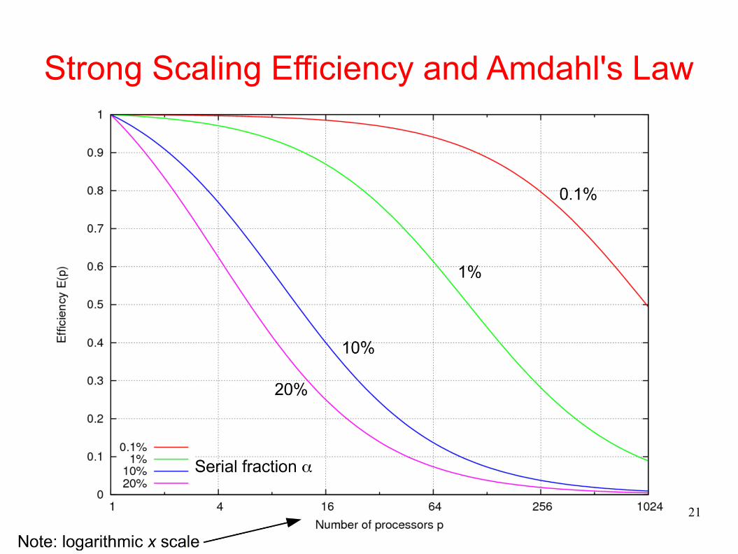
Strong Scaling Efficiency and Amdahl's Law
Performance Evaluation 22
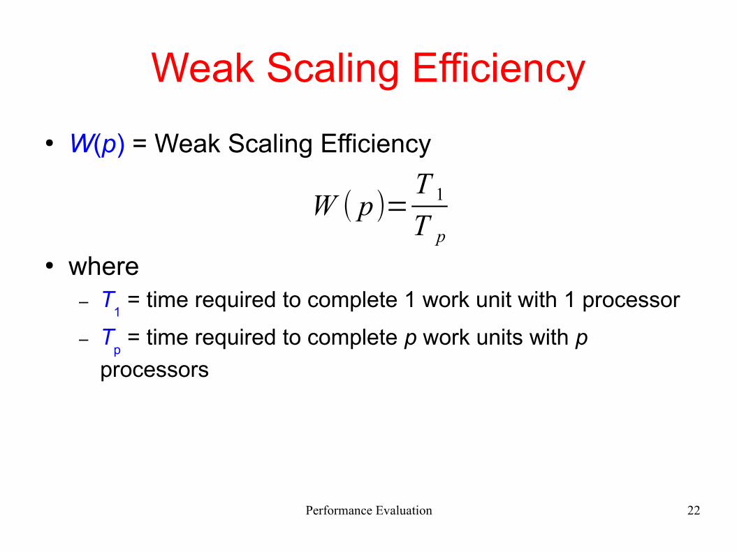
Weak Scaling Efficiency
● W(p) = Weak Scaling Efficiency
● where– T
1 = time required to complete 1 work unit with 1 processor
– Tp = time required to complete p work units with p
processors
W ( p)=T 1
T p
Performance Evaluation 23
Weak scaling
● Let f(np, p) be the amount of work done by each
processor, given input size np and p processors
● We want to compute the input size(s) np such that:
f(np, p) = constant
Performance Evaluation 24
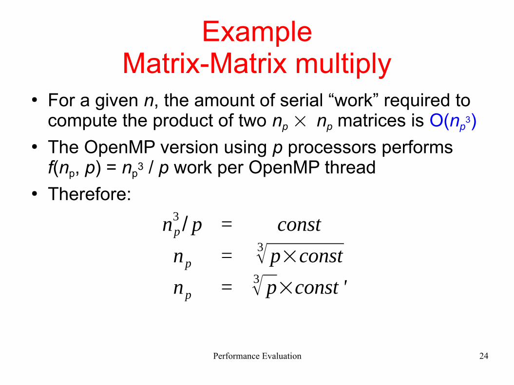
ExampleMatrix-Matrix multiply
● For a given n, the amount of serial “work” required to compute the product of two np ´ np matrices is O(np
3)● The OpenMP version using p processors performs
f(np, p) = np3 / p work per OpenMP thread
● Therefore:
np3/ p = const
np = 3√ p×const
np = 3√ p×const '
Performance Evaluation 25
Example
● See omp-matmul.c– demo-strong-scaling.sh computes the times required for
strong scaling (demo-strong-scaling.ods)– demo-weak-scaling.sh computes the times required for weak
scaling (demo-weak-scaling.ods)
Performance Evaluation 26
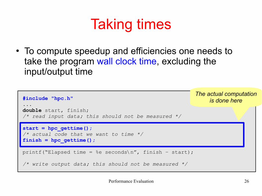
Taking times
● To compute speedup and efficiencies one needs to take the program wall clock time, excluding the input/output time
#include "hpc.h"...double start, finish;/* read input data; this should not be measured */
start = hpc_gettime(); /* actual code that we want to time */finish = hpc_gettime();
printf(“Elapsed time = %e seconds\n”, finish – start);
/* write output data; this should not be measured */
The actual computation is done here
Performance Evaluation 27
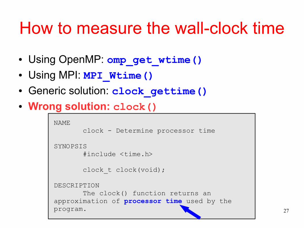
How to measure the wall-clock time
● Using OpenMP: omp_get_wtime()● Using MPI: MPI_Wtime()● Generic solution: clock_gettime()● Wrong solution: clock()
NAME clock - Determine processor time
SYNOPSIS #include <time.h>
clock_t clock(void);
DESCRIPTION The clock() function returns an approximation of processor time used by the program.
Performance Evaluation 28
Post Scriptum:How to present results
Performance Evaluation 29
Basic rules for graphing data
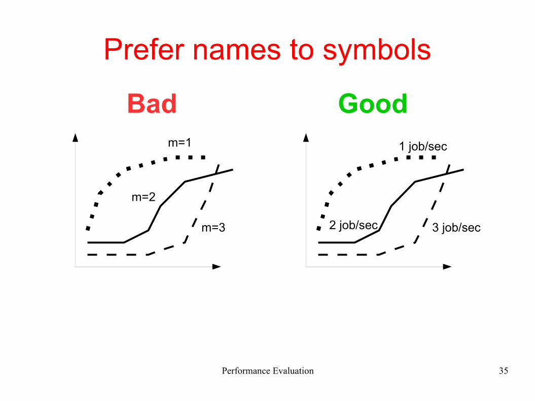
● Understanding the data should require the least possible effort from the reader– E.g., use names instead of symbols for the legend when
possible● Provide enough information to make the graph self-
contained● Stick to widely accepted practices
– The origin of plots should be (0, 0)– The effect should be on the y axis, the cause on the x axis

Performance Evaluation 30
Stick to accepted practices
Bad
https://www.buzzfeed.com/katienotopoulos/graphs-that-lied-to-us
Performance Evaluation 31
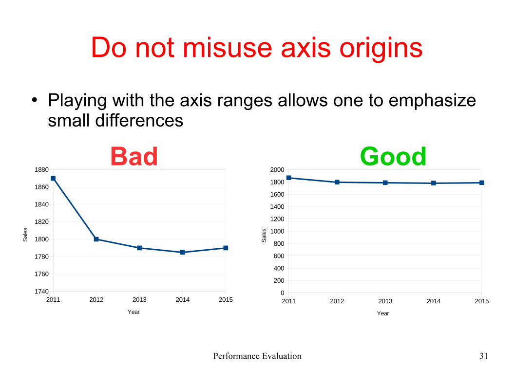
Do not misuse axis origins
● Playing with the axis ranges allows one to emphasize small differences
2011 2012 2013 2014 20151740
1760
1780
1800
1820
1840
1860
1880
Year
Sales
2011 2012 2013 2014 20150
200
400
600
800
1000
1200
1400
1600
1800
2000
Year
Sales
Bad Good
Performance Evaluation 33
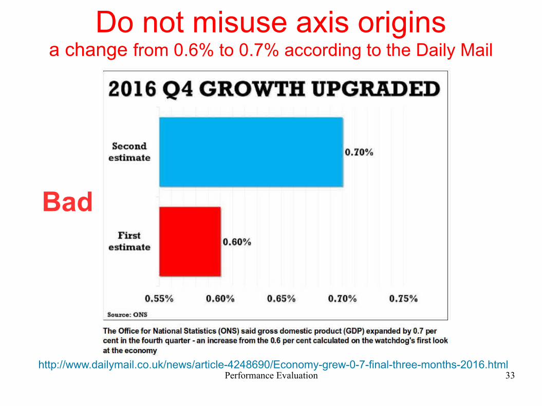
Do not misuse axis originsa change from 0.6% to 0.7% according to the Daily Mail
http://www.dailymail.co.uk/news/article-4248690/Economy-grew-0-7-final-three-months-2016.html
Bad
Performance Evaluation 34
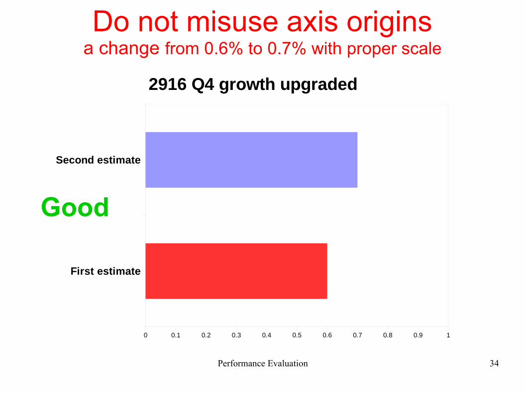
Do not misuse axis originsa change from 0.6% to 0.7% with proper scale
First estimate
Second estimate
0 0.1 0.2 0.3 0.4 0.5 0.6 0.7 0.8 0.9 1
2916 Q4 growth upgraded
Good
Performance Evaluation 35
Prefer names to symbols
m=1
m=2
m=3
1 job/sec
2 job/sec 3 job/sec
Bad Good
Performance Evaluation 36
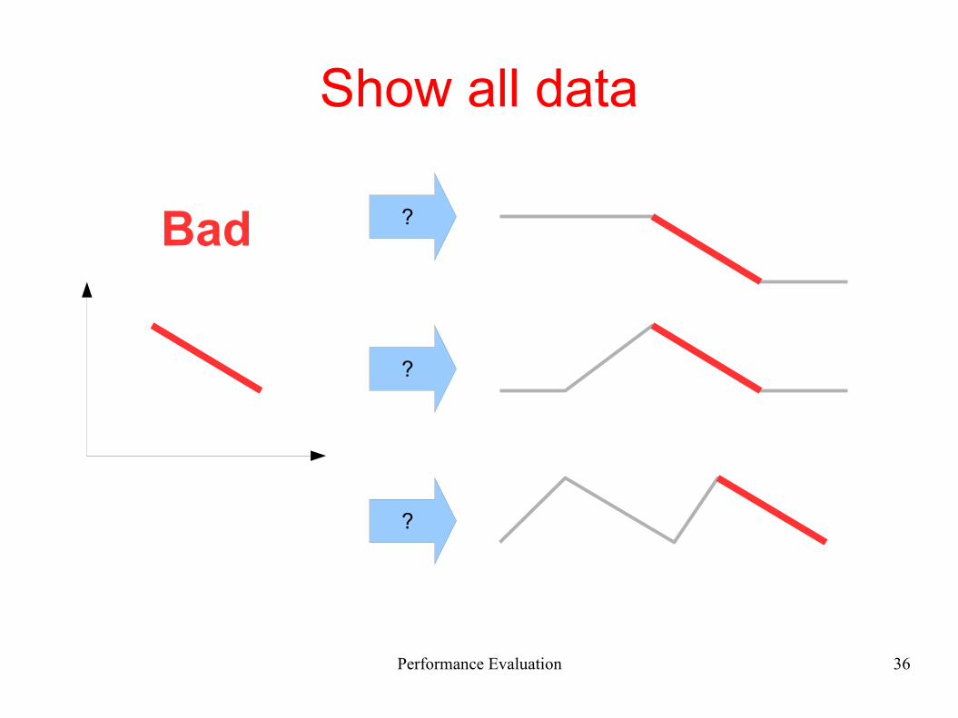
Show all data
?
Bad ?
?
Performance Evaluation 37
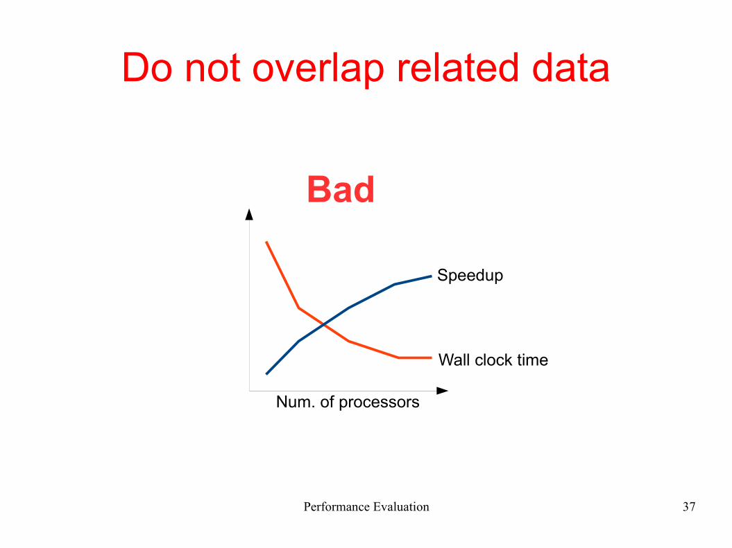
Do not overlap related data
Wall clock time
Speedup
Num. of processors
Bad
Performance Evaluation 38
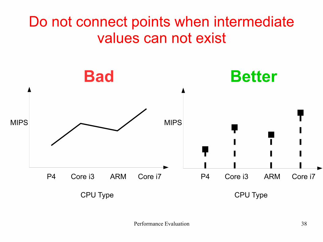
Do not connect points when intermediate values can not exist
MIPS
CPU Type
P4 Core i3 ARM Core i7
Bad
MIPS
CPU Type
P4 Core i3 ARM Core i7
Better
Performance Evaluation 39
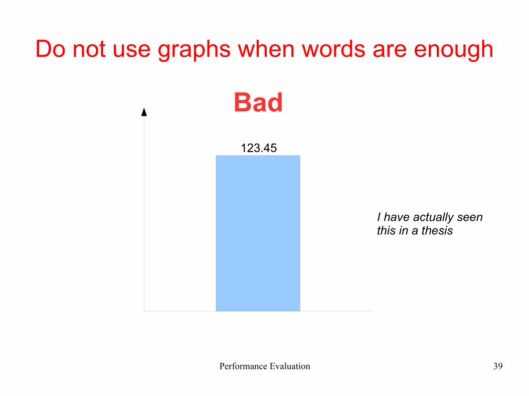
Do not use graphs when words are enough
123.45
Bad
I have actually seen this in a thesis
Performance Evaluation 40
Other suggestions
● Always add a (numbered) caption to each figure– If possible, the caption should contain enough information to
understand the figure without reading the main text● All figures must be referenced and described in the
main text of your document
Performance Evaluation 41
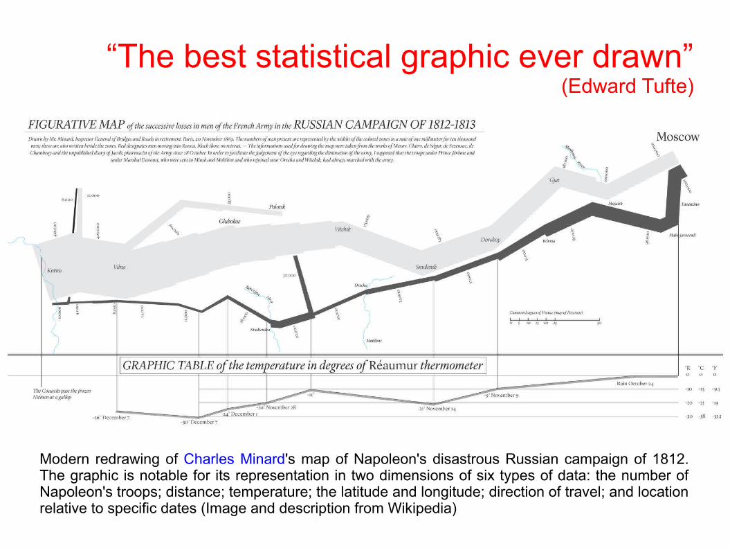
“The best statistical graphic ever drawn”(Edward Tufte)
Modern redrawing of Charles Minard's map of Napoleon's disastrous Russian campaign of 1812. The graphic is notable for its representation in two dimensions of six types of data: the number of Napoleon's troops; distance; temperature; the latitude and longitude; direction of travel; and location relative to specific dates (Image and description from Wikipedia)
Performance Evaluation 42
Suggested reading
Edward R. Tufte, The Visual Display of Quantitative Information, 2nd ed., Graphics Press, 2011, ISBN 978-0961392147
Recommended