
7/29/2019 Planning and Navigation for Robots
http://slidepdf.com/reader/full/planning-and-navigation-for-robots 1/47
6 - Planning and Navigation
© R. Siegwart, ETH Zurich - ASL
6
1 Today’s Outline
Path planning and navigation
Visual SLAM

7/29/2019 Planning and Navigation for Robots
http://slidepdf.com/reader/full/planning-and-navigation-for-robots 2/47
Autonomous Mobile Robots
Autonomous Systems LabZürich
Planning and
Navigation
Where am I?
Where am I going?
How do I get there?
"Position"
Global Map
Perception Motion Control
Cognition
Real WorldEnvironment
Localization
PathEnvironment ModelLocal Map
?
7/29/2019 Planning and Navigation for Robots
http://slidepdf.com/reader/full/planning-and-navigation-for-robots 3/47
6 - Planning and Navigation
© R. Siegwart, ETH Zurich - ASL
6
3 Competencies for Navigation I
Cognition / Reasoning :
is the ability to decide what actions are required to achieve a certain goal in
a given situation (belief state).
decisions ranging from what path to take to what information on theenvironment to use.
Today’s industrial robots can operate without any cognition (reasoning)
because their environment is static and very structured.
In mobile robotics, cognition and reasoning is primarily of geometric
nature, such as picking safe path or determining where to go next.
already been largely explored in literature for cases in which complete
information about the current situation and the environment exists (e.g. sales
man problem).
7/29/2019 Planning and Navigation for Robots
http://slidepdf.com/reader/full/planning-and-navigation-for-robots 4/47
6 - Planning and Navigation
© R. Siegwart, ETH Zurich - ASL
6
4 Competencies for Navigation II
However, in mobile robotics the knowledge of about the environment and
situation is usually only partially known and is uncertain.
makes the task much more difficult
requires multiple tasks running in parallel, some for planning (global), some toguarantee “survival of the robot”.
Robot control can usually be decomposed in various behaviors or
functions
e.g. wall following, localization, path generation or obstacle avoidance.
In this chapter we are concerned with path planning and navigation, except
the low lever motion control and localization.
We can generally distinguish between (global) path planning and (local)
obstacle avoidance.
7/29/2019 Planning and Navigation for Robots
http://slidepdf.com/reader/full/planning-and-navigation-for-robots 5/47
6 - Planning and Navigation
© R. Siegwart, ETH Zurich - ASL
6
5 Path Planning
The problem: find a path in the phisical space from the initial position to the
goal position avoiding all collisions with the obstacles
We can generally distinguish between
(global) path planning and
(local) obstacle avoidance.

7/29/2019 Planning and Navigation for Robots
http://slidepdf.com/reader/full/planning-and-navigation-for-robots 6/47
6 - Planning and Navigation
© R. Siegwart, ETH Zurich - ASL
6
6 Global Path Planing
Assumption: there exists a good enough map of the environment for
navigation.
Topological or metric or a mixture between both.
First step:
Representation of the environment by a road-map (graph), cells or a potential
field. The resulting discrete locations or cells allow then to use standard
planning algorithms.
Examples that we will see:
Visibility Graph
Voronoi Diagram
Cell Decomposition -> Connectivity Graph
Potential Field
7/29/2019 Planning and Navigation for Robots
http://slidepdf.com/reader/full/planning-and-navigation-for-robots 7/47
6 - Planning and Navigation
© R. Siegwart, ETH Zurich - ASL
6
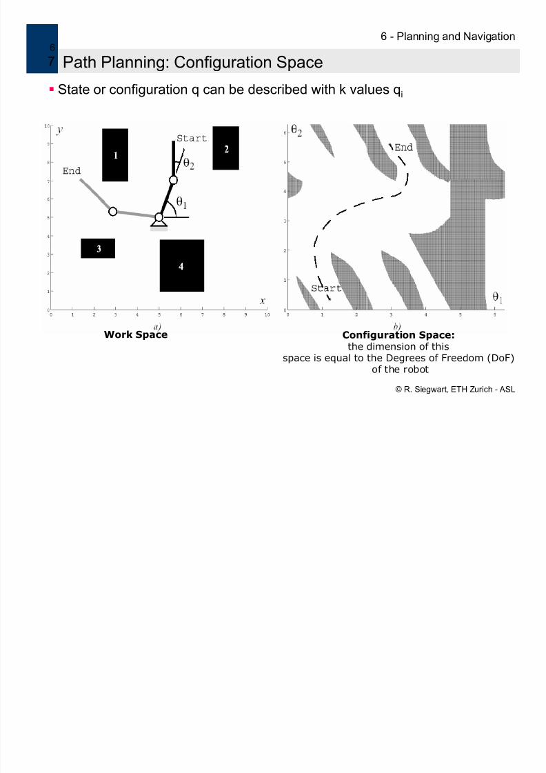
7 Path Planning: Configuration Space
State or configuration q can be described with k values qi
What is the configuration space of a mobile robot?
Work Space Configuration Space:the dimension of this
space is equal to the Degrees of Freedom (DoF)
of the robot

7/29/2019 Planning and Navigation for Robots
http://slidepdf.com/reader/full/planning-and-navigation-for-robots 8/47
6 - Planning and Navigation
© R. Siegwart, ETH Zurich - ASL
6
8 Configuration Space for a Mobile Robot
Mobile robots operating on a flat ground have 3 DoF: (x, y, θ)
For simplification, mobile roboticists assume that the robot is a point. In
this way the configuration space is reduced to 2D (x,y)
Because we have reduced each robot to a point, we have to inflate each
obsttacle by the size of the robot radius to compensate.
7/29/2019 Planning and Navigation for Robots
http://slidepdf.com/reader/full/planning-and-navigation-for-robots 9/47
6 - Planning and Navigation
© R. Siegwart, ETH Zurich - ASL
6
9 Path Planning Overview
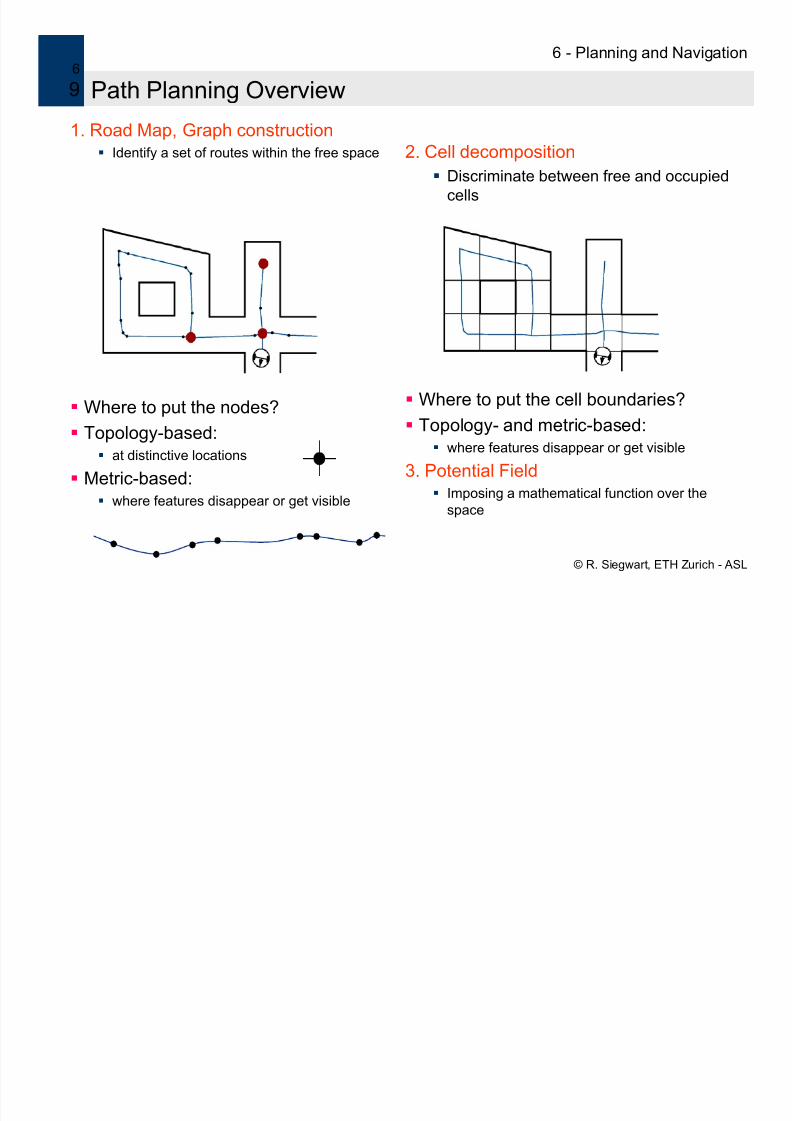
1. Road Map, Graph construction
Identify a set of routes within the free space
Where to put the nodes?
Topology-based: at distinctive locations
Metric-based:
where features disappear or get visible
2. Cell decomposition
Discriminate between free and occupied
cells
Where to put the cell boundaries?
Topology- and metric-based:
where features disappear or get visible
3. Potential Field
Imposing a mathematical function over the
space
7/29/2019 Planning and Navigation for Robots
http://slidepdf.com/reader/full/planning-and-navigation-for-robots 10/47
6 - Planning and Navigation
© R. Siegwart, ETH Zurich - ASL
6
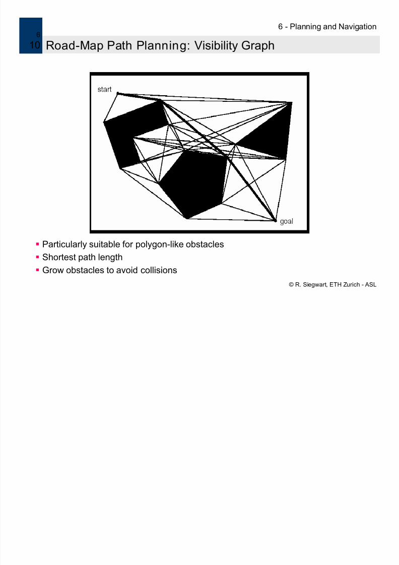
10 Road-Map Path Planning: Visibility Graph
Particularly suitable for polygon-like obstacles
Shortest path length
Grow obstacles to avoid collisions

7/29/2019 Planning and Navigation for Robots
http://slidepdf.com/reader/full/planning-and-navigation-for-robots 11/47
6 - Planning and Navigation
© R. Siegwart, ETH Zurich - ASL
6
11 Visibility Graph
Pros
It is easy to find the shortest path from the start to the goal positions
Implementation simple when obstacles are polygons
Cons
Number of edges and nodes increases with the number of polygons
Thus it can be inefficient in densely populated environments
The solution path found by the visibility graph tend to take the robot asclose aspossible to obstacles: the common solution is to grow obstacles by more than
robot’s radius

7/29/2019 Planning and Navigation for Robots
http://slidepdf.com/reader/full/planning-and-navigation-for-robots 12/47
6 - Planning and Navigation
© R. Siegwart, ETH Zurich - ASL
6
12 Road-Map Path Planning: Voronoi Diagram
In contrast to the Visibility Graph approach tends to maximize the distancebetween robot and obstacles
Easy executable: Maximize the sensor readings
Works also for map-building: Move on the Voronoi edges Sysquake Demo

7/29/2019 Planning and Navigation for Robots
http://slidepdf.com/reader/full/planning-and-navigation-for-robots 13/47
6 - Planning and Navigation
© R. Siegwart, ETH Zurich - ASL
6
13 Voronoi Diagram
Pros
Using range sensors like laser or sonar, a robot can navigate along the Voronoi
diagram using simple control rules
Cons
Because the Voronoi diagram tends to keep the robot as far as possible from
obstacles, any short range sensor will be in danger of failing
Peculiarities
when obstacles are polygons, the Voronoi map consists of straight and
parabolic segments
7/29/2019 Planning and Navigation for Robots
http://slidepdf.com/reader/full/planning-and-navigation-for-robots 14/47
6 - Planning and Navigation
© R. Siegwart, ETH Zurich - ASL
6
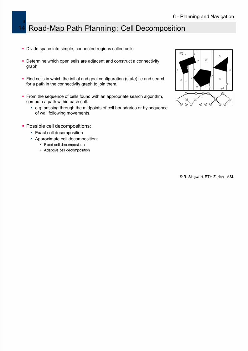
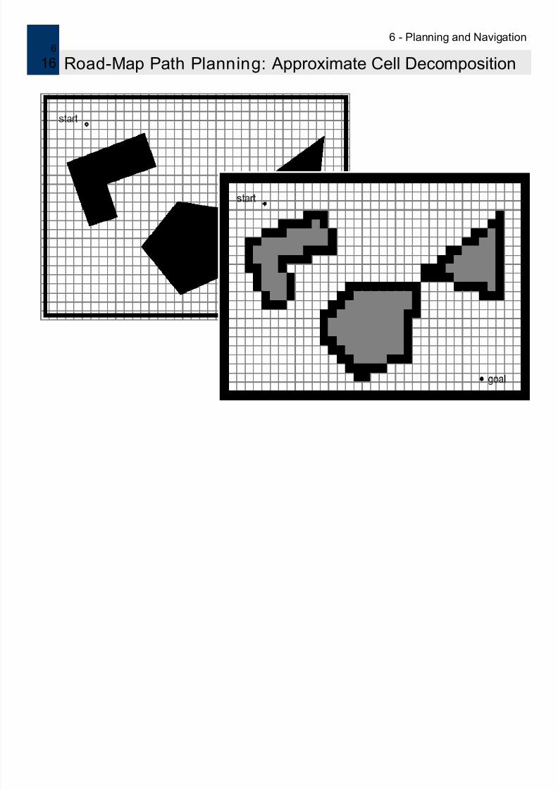
14 Road-Map Path Planning: Cell Decomposition
Divide space into simple, connected regions called cells
Determine which open sells are adjacent and construct a connectivity
graph
Find cells in which the initial and goal configuration (state) lie and search
for a path in the connectivity graph to join them.
From the sequence of cells found with an appropriate search algorithm,
compute a path within each cell. e.g. passing through the midpoints of cell boundaries or by sequence
of wall following movements.
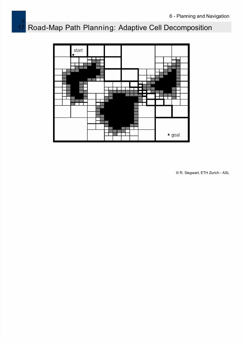
Possible cell decompositions:
Exact cell decomposition Approximate cell decomposition:
• Fixed cell decomposition
• Adaptive cell decomposition
7/29/2019 Planning and Navigation for Robots
http://slidepdf.com/reader/full/planning-and-navigation-for-robots 15/47
6 - Planning and Navigation
© R. Siegwart, ETH Zurich - ASL
6
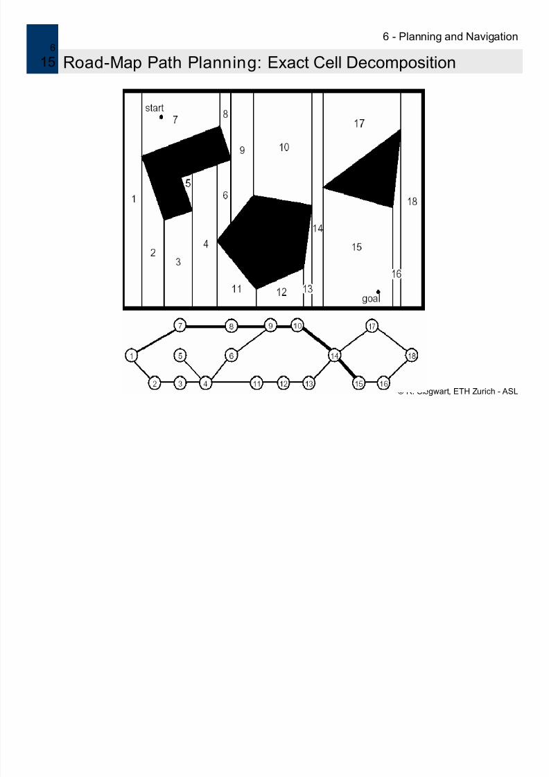
15 Road-Map Path Planning: Exact Cell Decomposition
7/29/2019 Planning and Navigation for Robots
http://slidepdf.com/reader/full/planning-and-navigation-for-robots 16/47
6 - Planning and Navigation
© R. Siegwart, ETH Zurich - ASL
6
16 Road-Map Path Planning: Approximate Cell Decomposition
7/29/2019 Planning and Navigation for Robots
http://slidepdf.com/reader/full/planning-and-navigation-for-robots 17/47
6 - Planning and Navigation
© R. Siegwart, ETH Zurich - ASL
6
17 Road-Map Path Planning: Adaptive Cell Decomposition
7/29/2019 Planning and Navigation for Robots
http://slidepdf.com/reader/full/planning-and-navigation-for-robots 18/47
6 - Planning and Navigation
© R. Siegwart, ETH Zurich - ASL
6
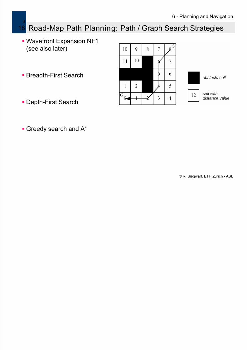
18 Road-Map Path Planning: Path / Graph Search Strategies
Wavefront Expansion NF1
(see also later)
Breadth-First Search
Depth-First Search
Greedy search and A*
7/29/2019 Planning and Navigation for Robots
http://slidepdf.com/reader/full/planning-and-navigation-for-robots 19/47
6 - Planning and Navigation
© R. Siegwart, ETH Zurich - ASL
6
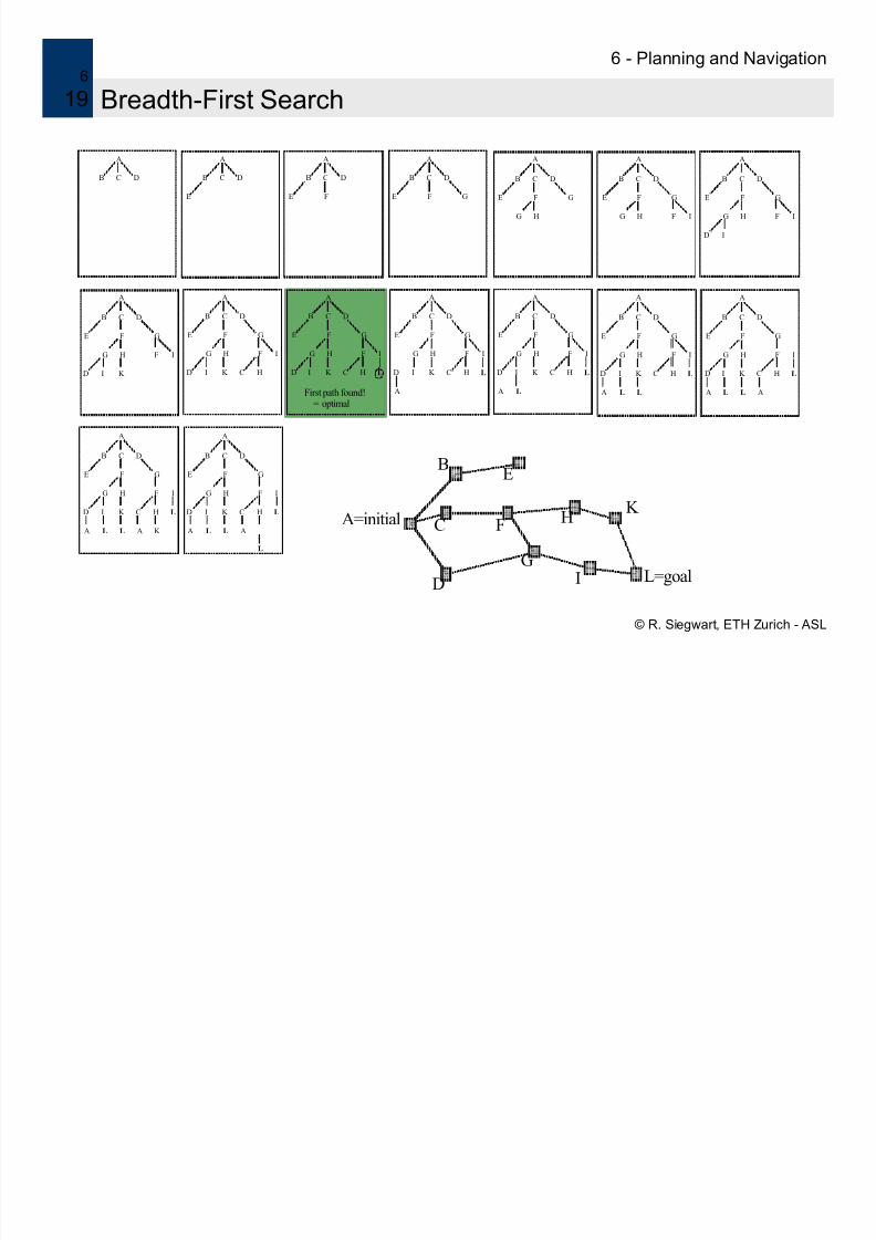
19 Breadth-First Search
B C D
A
E
B C D
A
FE
B C D
A
GFE
B C D
A
F
G
G H I
FE
B C D
A
F
G
ID
G H I
FE
B C D
A
F
G
I K D
G H I
FE
B C D
A
H
F
G
I K CD
G H I
FE
B C D
A
H
F
G
I K CD L
A
G H I
FE
B C D
A
H
F
G
I K CD L
LA
G H I
FE
B C D
A
H
F
G
I K CD L
L LA
G H I
FE
B C D
A
H
F
G
I K CD L
L L AA
G H I
FE
B C D
A
H
K
F
G
I K CD L
L L AA
G H I
FE
B C D
A
H
F
G
I K CD L
L L AA
L
G H I
FE
B C D
A
A=initial
B
C
D
F
G
H
I
K
L=goal
E
H
F
G
I K CD L
G H I
FE
B C D
A
First path found!= optimal
G
G H
FE
B C D
A
7/29/2019 Planning and Navigation for Robots
http://slidepdf.com/reader/full/planning-and-navigation-for-robots 20/47
6 - Planning and Navigation
© R. Siegwart, ETH Zurich - ASL
6
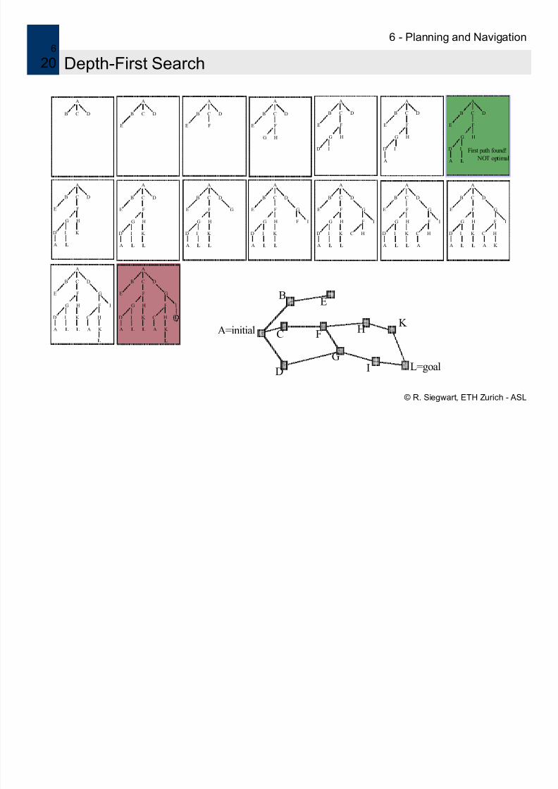
20 Depth-First Search
B C D
A
E
B C D
A
FE
B C D
A
G H
FE
B C D
A
ID
G H
FE
B C D
A
D
A
G H
FE
B C D
A
I
I K D
LA
G H
FE
B C D
A
ID
LA
G H
FE
B C D
A
First path found! NOT optimal
I K D
L LA
G H
FE
B C D
A
G
I K D
L LA
G H
FE
B C D
A
F
G
I K D
L LA
G H I
FE
B C D
A
H
F
G
I K CD
L LA
G H I
FE
B C D
A
H
F
G
I K CD
L L AA
G H I
FE
B C D
A
H
K
F
G
I K CD
L L AA
G H I
FE
B C D
A
H
K
F
G
I K CD
L L AA
L
G H I
FE
B C D
A
H
K
F
G
I K CD L
L L AA
L
G H I
FE
B C D
A
A=initial
B
C
D
F
G
H
I
K
L=goal
E
7/29/2019 Planning and Navigation for Robots
http://slidepdf.com/reader/full/planning-and-navigation-for-robots 21/47
6 - Planning and Navigation
© R. Siegwart, ETH Zurich - ASL
6
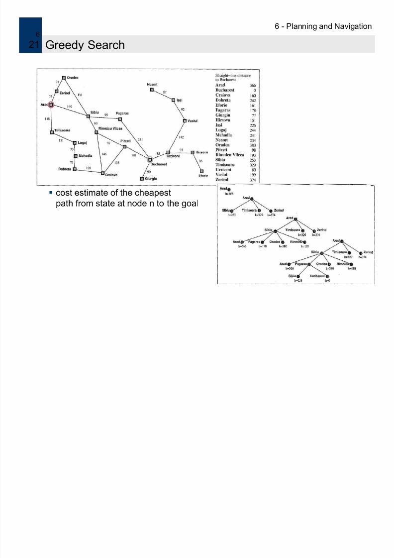
21 Greedy Search
h(n) = straight-line distance
cost estimate of the cheapest
path from state at node n to the goal
7/29/2019 Planning and Navigation for Robots
http://slidepdf.com/reader/full/planning-and-navigation-for-robots 22/47
6 - Planning and Navigation
© R. Siegwart, ETH Zurich - ASL
6
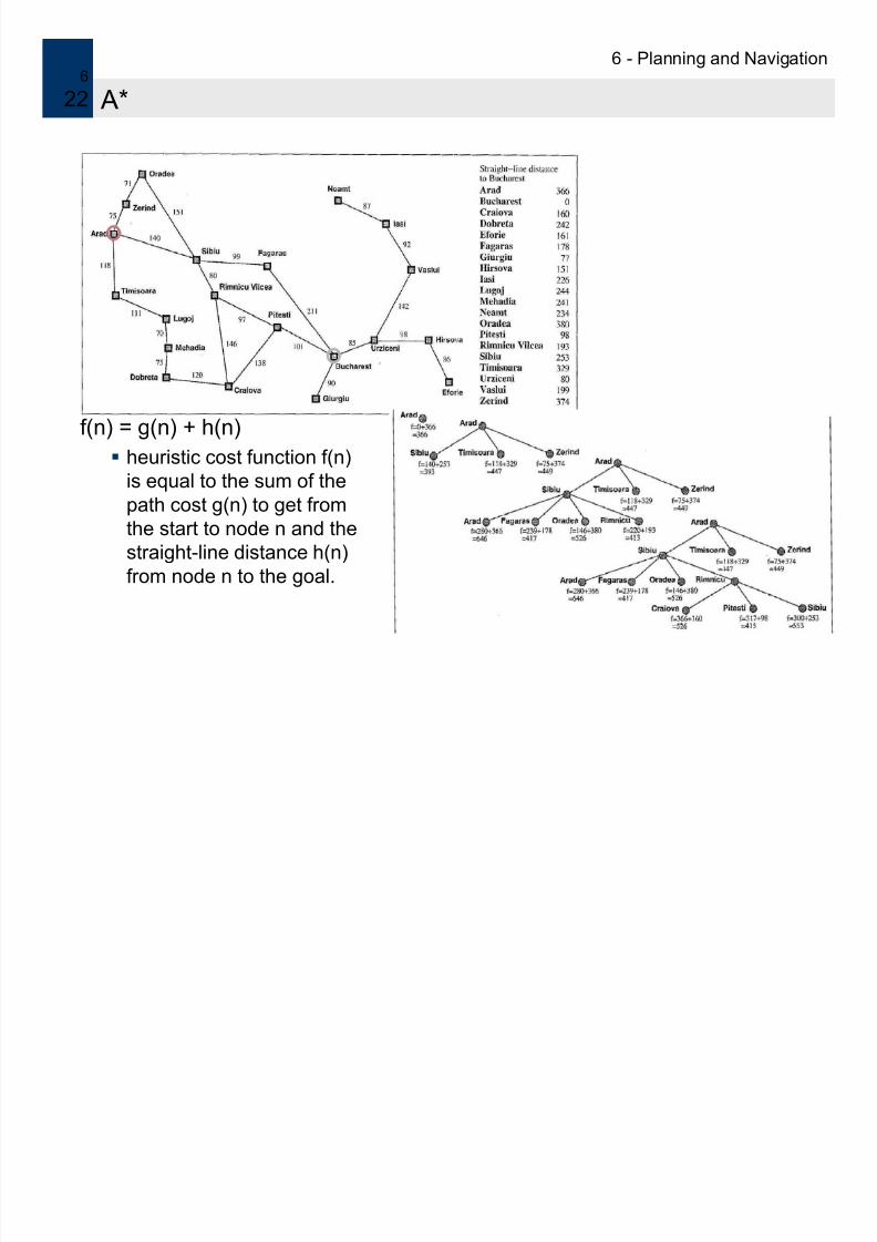
22 A*
f (n) = g(n) + h(n)
heuristic cost function f(n)
is equal to the sum of thepath cost g(n) to get from
the start to node n and the
straight-line distance h(n)
from node n to the goal.
7/29/2019 Planning and Navigation for Robots
http://slidepdf.com/reader/full/planning-and-navigation-for-robots 23/47
6 - Planning and Navigation
© R. Siegwart, ETH Zurich - ASL
6
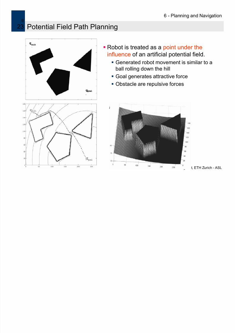
23 Potential Field Path Planning
Robot is treated as a point under the
influence of an artificial potential field.
Generated robot movement is similar to aball rolling down the hill
Goal generates attractive force
Obstacle are repulsive forces

7/29/2019 Planning and Navigation for Robots
http://slidepdf.com/reader/full/planning-and-navigation-for-robots 24/47
6 - Planning and Navigation
© R. Siegwart, ETH Zurich - ASL
6
24 Potential Field Path Planning: Potential Field Generation
Generation of potential field function U(q)
attracting (goal) and repulsing (obstacle) fields
summing up the fields
functions must be differentiable Generate artificial force field F(q)
Set robot speed (vx, vy) proportional to the force F(q) generated by the field
the force field drives the robot to the goal
if robot is assumed to be a point mass
⎥⎥
⎥⎥
⎦
⎤
⎢⎢
⎢⎢
⎣
⎡
∂
∂∂
∂
=∇−−∇=−∇=
y
U x
U
qU qU qU qF repatt )()()()(
7/29/2019 Planning and Navigation for Robots
http://slidepdf.com/reader/full/planning-and-navigation-for-robots 25/47
6 - Planning and Navigation
© R. Siegwart, ETH Zurich - ASL
6
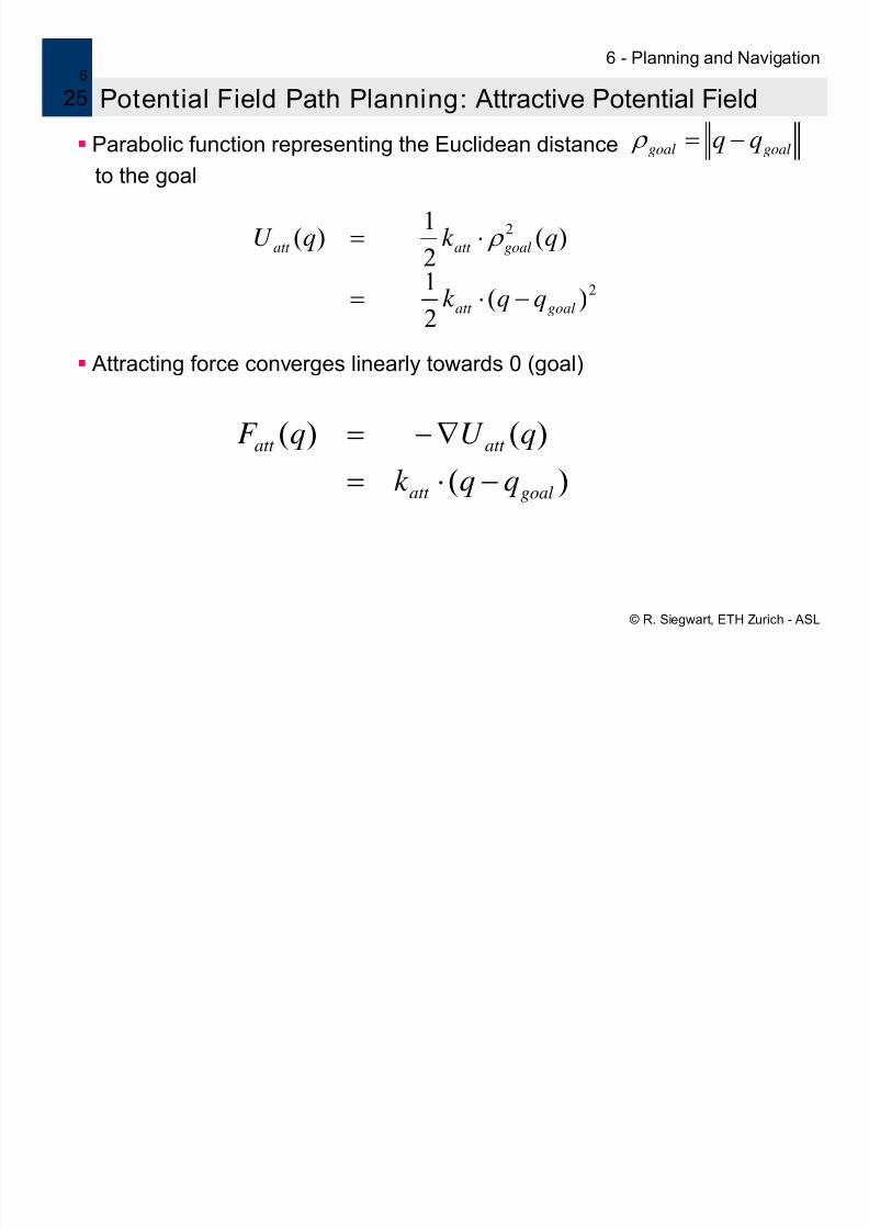
25 Potential Field Path Planning: Attractive Potential Field
Parabolic function representing the Euclidean distance
to the goal
Attracting force converges linearly towards 0 (goal)
goalgoal qq −= ρ
)(
)()(
goalatt
att att
qqk
qU qF
−⋅=
∇−=
2
2
)(2
1
)(2
1
)(
goalatt
goalatt att
qqk
qk qU
−⋅=
⋅= ρ

7/29/2019 Planning and Navigation for Robots
http://slidepdf.com/reader/full/planning-and-navigation-for-robots 26/47
6 - Planning and Navigation
© R. Siegwart, ETH Zurich - ASL
6
26 Potential Field Path Planning: Repulsing Potential Field
Should generate a barrier around all the obstacle
strong if close to the obstacle
not influence if fare from the obstacle
: minimum distance to the object
Field is positive or zero and tends to infinity as q gets closer to the object
obst.
7/29/2019 Planning and Navigation for Robots
http://slidepdf.com/reader/full/planning-and-navigation-for-robots 27/47
6 - Planning and Navigation
© R. Siegwart, ETH Zurich - ASL
6
27 Potential Field Path Planning:
Notes:
Local minima problem exists
problem is getting more complex if the robot is not considered as a point mass
If objects are convex there exists situations where several minimal distancesexist → can result in oscillations
Sysquake Demo
The Demo can also be seen at:
http://www.k-team.com/kteam/index.php?page=174&rub=&site=1

7/29/2019 Planning and Navigation for Robots
http://slidepdf.com/reader/full/planning-and-navigation-for-robots 28/47
7/29/2019 Planning and Navigation for Robots
http://slidepdf.com/reader/full/planning-and-navigation-for-robots 29/47
6 - Planning and Navigation
© R. Siegwart, ETH Zurich - ASL
6
29 Potential Field Path Planning: Potential Field using a Dyn. Model
Forces in the polar plane
no time consuming transformations
Robot modeled thoroughly
potential field forces directly acting on the model
filters the movement -> smooth
Local minima
set a new goal point
Monatana et at.
7/29/2019 Planning and Navigation for Robots
http://slidepdf.com/reader/full/planning-and-navigation-for-robots 30/47
6 - Planning and Navigation
© R. Siegwart, ETH Zurich - ASL
6
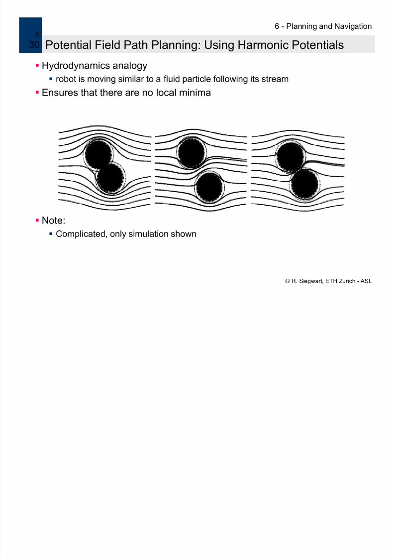
30 Potential Field Path Planning: Using Harmonic Potentials
Hydrodynamics analogy
robot is moving similar to a fluid particle following its stream
Ensures that there are no local minima
Note:
Complicated, only simulation shown

7/29/2019 Planning and Navigation for Robots
http://slidepdf.com/reader/full/planning-and-navigation-for-robots 31/47
Autonomous Mobile Robots
Autonomous Systems LabZürich
Real Time 3D SLAM with a Single Camera
This presentation is based on the following papers:
• Andrew J. Davison, Real-Time Simultaneous Localization and Mapping with a Single Camera , ICCV 2003
•Nicholas Molton, Andrew J. Davison and Ian Reid, Locally Planar Patch Features for Real-Time Structure
from Motion, BMVC 2004

7/29/2019 Planning and Navigation for Robots
http://slidepdf.com/reader/full/planning-and-navigation-for-robots 32/47
6 - Planning and Navigation
© R. Siegwart, ETH Zurich - ASL
6
32 Outline
Visual SLAM versus Structure From Motion
Extended Kalman Filter for First-Order Uncertainty Propagation Camera Motion Model
Matching of Existing Features
Initialization of new features in the map
Improving feature matching
6 Pl i d N i ti

7/29/2019 Planning and Navigation for Robots
http://slidepdf.com/reader/full/planning-and-navigation-for-robots 33/47
6 - Planning and Navigation
© R. Siegwart, ETH Zurich - ASL
6
33
Structure from Motion:
Take some images of the object toreconstruct
Features (points, lines, …) areextracted from all frames andmatched among them
All images are processedsimultaneously
Both camera motion and 3D structurecan be recovered by optimally fusingthe overall information, up to a scalefactor
Robust solution but far frombeing Real-Time !
Structure From Motion (SFM)
6 Pl i d N i ti
7/29/2019 Planning and Navigation for Robots
http://slidepdf.com/reader/full/planning-and-navigation-for-robots 34/47
6 - Planning and Navigation
© R. Siegwart, ETH Zurich - ASL
6
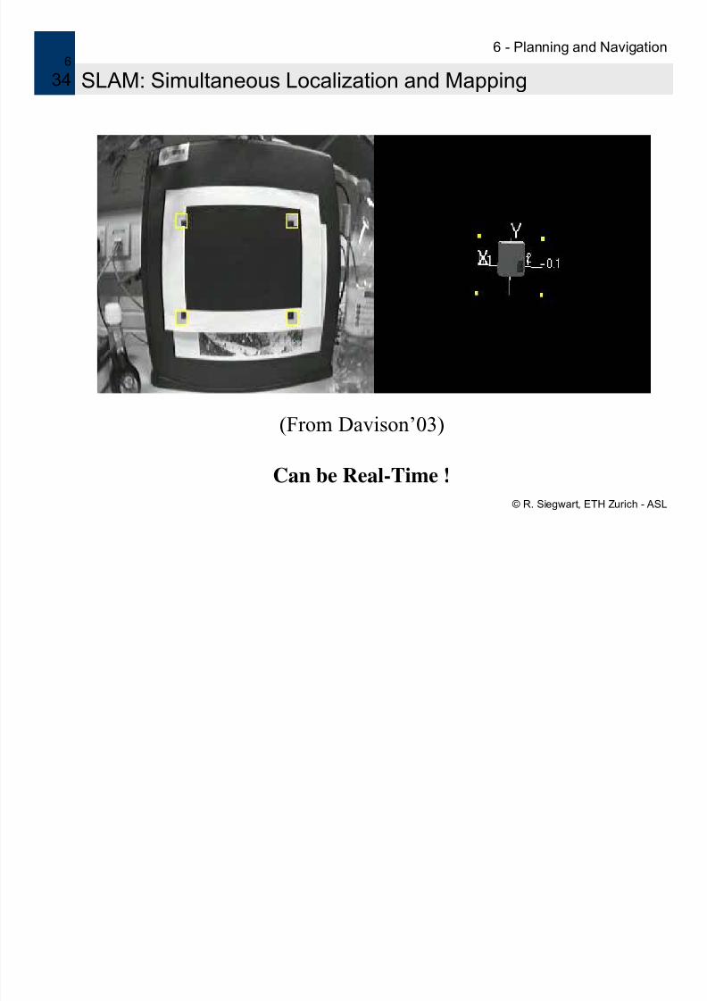
34 SLAM: Simultaneous Localization and Mapping
(From Davison’03)
Can be Real-Time !
6 Planning and Navigation

7/29/2019 Planning and Navigation for Robots
http://slidepdf.com/reader/full/planning-and-navigation-for-robots 35/47
6 - Planning and Navigation
© R. Siegwart, ETH Zurich - ASL
6
35 SLAM versus SFM
Repeatable Localization
Ability to estimate the location of the camera after 10 minutes of motion with the same
accuracy as was possible after 10 seconds.
Features must be stable, long-term landmark, no transient (as in SFM)
6 Planning and Navigation
7/29/2019 Planning and Navigation for Robots
http://slidepdf.com/reader/full/planning-and-navigation-for-robots 36/47
6 - Planning and Navigation
© R. Siegwart, ETH Zurich - ASL
6
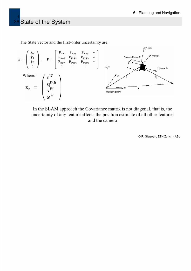
36 State of the System
The State vector and the first-order uncertainty are:
Where:
In the SLAM approach the Covariance matrix is not diagonal, that is, the
uncertainty of any feature affects the position estimate of all other features
and the camera
6 - Planning and Navigation
7/29/2019 Planning and Navigation for Robots
http://slidepdf.com/reader/full/planning-and-navigation-for-robots 37/47
6 - Planning and Navigation
© R. Siegwart, ETH Zurich - ASL
6
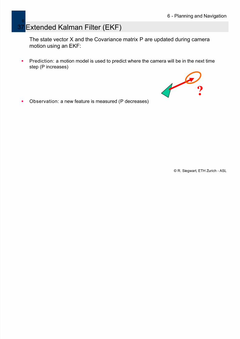
37 Extended Kalman Filter (EKF)
The state vector X and the Covariance matrix P are updated during camera
motion using an EKF:
Prediction: a motion model is used to predict where the camera will be in the next time
step (P increases)
Observation: a new feature is measured (P decreases)
?
6 - Planning and Navigation

7/29/2019 Planning and Navigation for Robots
http://slidepdf.com/reader/full/planning-and-navigation-for-robots 38/47
6 Planning and Navigation
© R. Siegwart, ETH Zurich - ASL
6
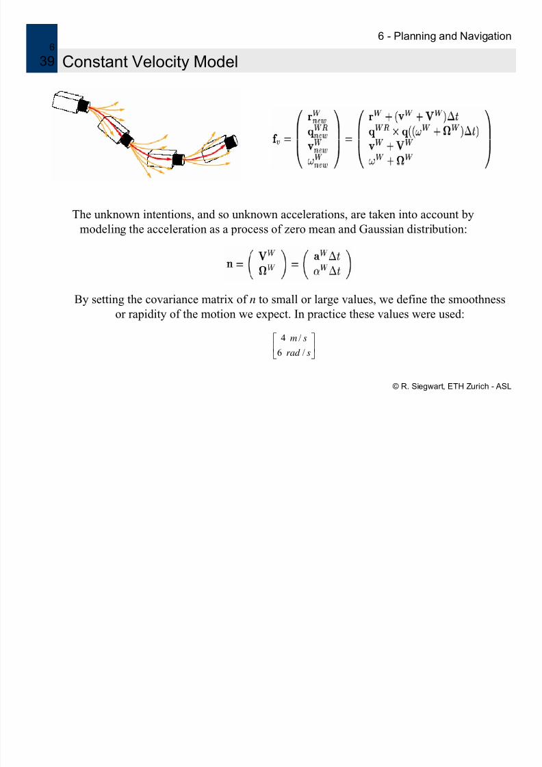
38 A Motion Model for Smoothly Moving Camera
Attempts to predict where the camera will be in the next time step
In the case the camera is attached to a person, the unknown intentions of the person can be statistically modeled
Most Structure from Motion approaches did not use any motion model!
7/29/2019 Planning and Navigation for Robots
http://slidepdf.com/reader/full/planning-and-navigation-for-robots 39/47

7/29/2019 Planning and Navigation for Robots
http://slidepdf.com/reader/full/planning-and-navigation-for-robots 40/47
6 - Planning and Navigation
7/29/2019 Planning and Navigation for Robots
http://slidepdf.com/reader/full/planning-and-navigation-for-robots 41/47
g g
© R. Siegwart, ETH Zurich - ASL
6
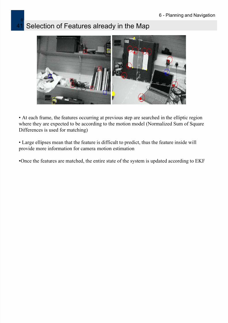
41 Selection of Features already in the Map
• At each frame, the features occurring at previous step are searched in the elliptic region
where they are expected to be according to the motion model (Normalized Sum of SquareDifferences is used for matching)
• Large ellipses mean that the feature is difficult to predict, thus the feature inside will
provide more information for camera motion estimation
•Once the features are matched, the entire state of the system is updated according to EKF
6 - Planning and Navigation
7/29/2019 Planning and Navigation for Robots
http://slidepdf.com/reader/full/planning-and-navigation-for-robots 42/47
g g
© R. Siegwart, ETH Zurich - ASL
6
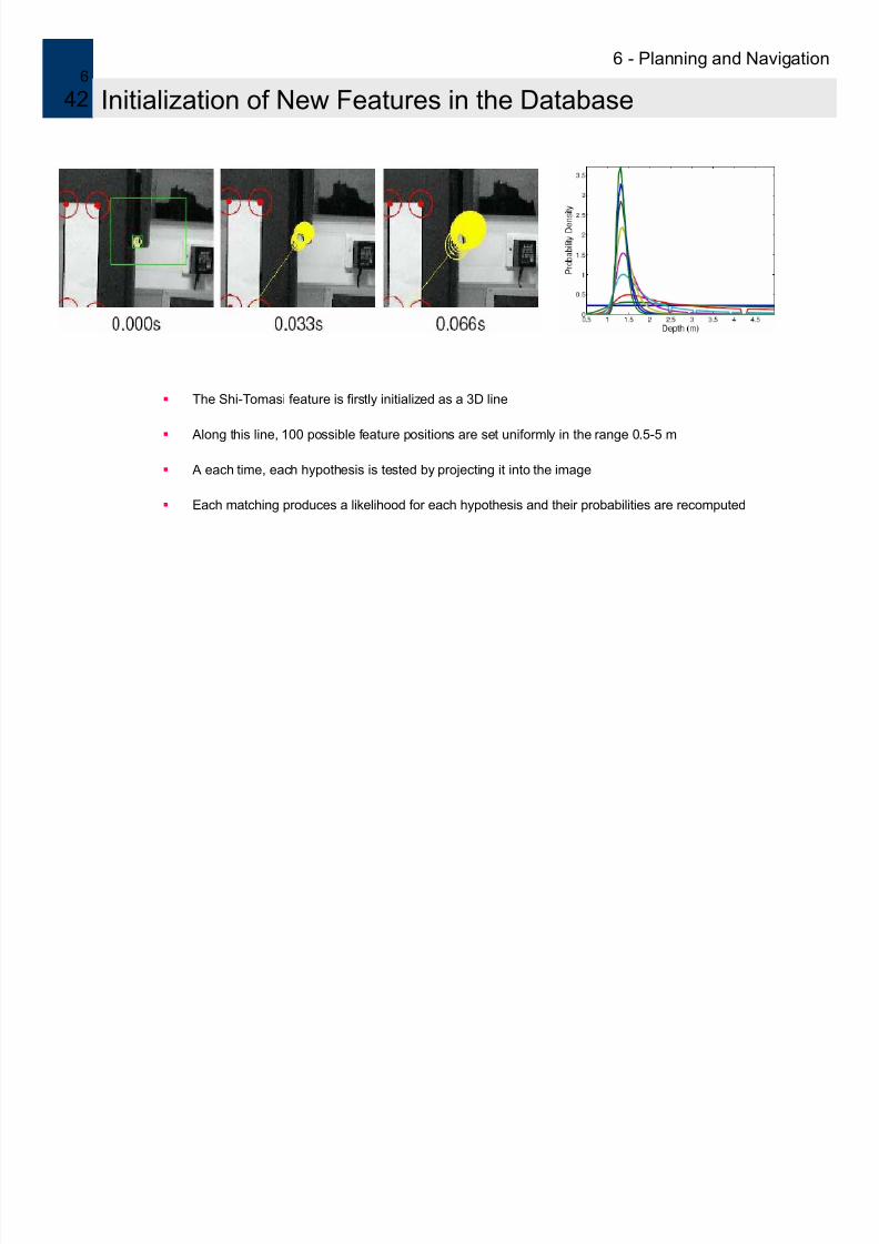
42 Initialization of New Features in the Database
The Shi-Tomasi feature is firstly initialized as a 3D line
Along this line, 100 possible feature positions are set uniformly in the range 0.5-5 m
A each time, each hypothesis is tested by projecting it into the image
Each matching produces a likelihood for each hypothesis and their probabilities are recomputed
6 - Planning and Navigation
7/29/2019 Planning and Navigation for Robots
http://slidepdf.com/reader/full/planning-and-navigation-for-robots 43/47
© R. Siegwart, ETH Zurich - ASL
6
43 Map Management
The number of features to be constantly visible in the image varies (in practice between 6-
10) according to• Localization accuracy
• Computing power available
If a feature is required to be added, the detected feature is added only if it is not expectedto disappear from the next image
A feature is deleted if it produces 50% of mismatches when it should be visible
6 - Planning and Navigation6

7/29/2019 Planning and Navigation for Robots
http://slidepdf.com/reader/full/planning-and-navigation-for-robots 44/47
© R. Siegwart, ETH Zurich - ASL
6
44 Improved Feature Matching
Up to now, tracked features were treated as 2D templates in image space
Long-term tracking can be improved by approximating the feature as a locally
planar region on 3D world surfaces
6 - Planning and Navigation6
7/29/2019 Planning and Navigation for Robots
http://slidepdf.com/reader/full/planning-and-navigation-for-robots 45/47
© R. Siegwart, ETH Zurich - ASL
6
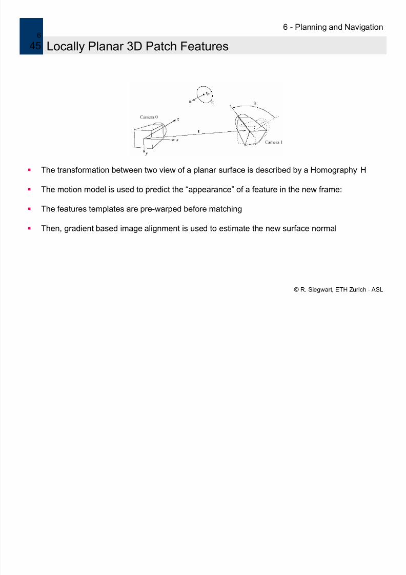
45 Locally Planar 3D Patch Features
The transformation between two view of a planar surface is described by a Homography H
The motion model is used to predict the “appearance” of a feature in the new frame:
The features templates are pre-warped before matching
Then, gradient based image alignment is used to estimate the new surface normal
6 - Planning and Navigation6

7/29/2019 Planning and Navigation for Robots
http://slidepdf.com/reader/full/planning-and-navigation-for-robots 46/47
© R. Siegwart, ETH Zurich - ASL
6
46 Locally Planar 3D Patch Features
6 - Planning and Navigation6

7/29/2019 Planning and Navigation for Robots
http://slidepdf.com/reader/full/planning-and-navigation-for-robots 47/47
© R. Siegwart, ETH Zurich - ASL
6
47 References
A. J. Davison, Real-Time Simultaneous Localization and Mapping with a Single Camera, ICCV 2003
N. Molton, A. J. Davison and I. Reid, Locally Planar Patch Features for Real-Time Structure from Motion, BMVC 2004
A. J. Davison, Y. Gonzalez Cid, N. Kita, Real-Time 3D SLAM with wide-angle vision, IFAC Symposium on Intelligent
Autonomous Vehicles, 2004
J. Shi and C. Tomasi, Good features to track, CVPR, 1994.
Recommended