1
Population Genetics 3:
Inbreeding
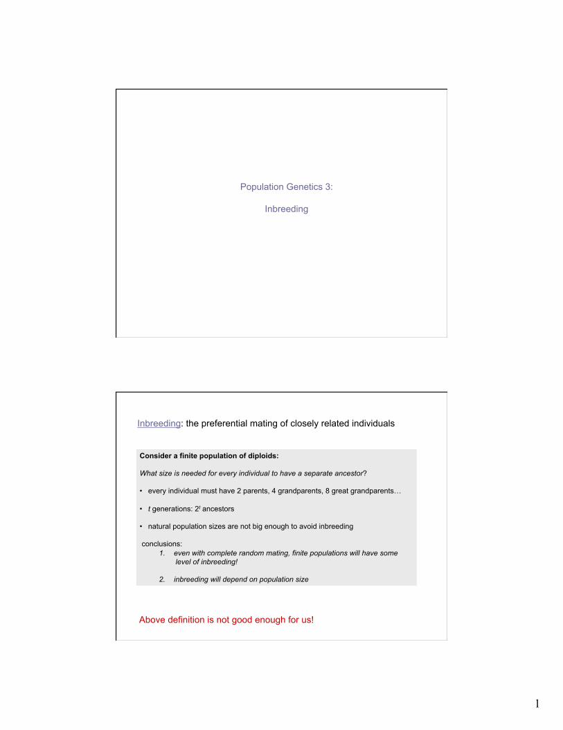
Inbreeding: the preferential mating of closely related individuals
Consider a finite population of diploids: What size is needed for every individual to have a separate ancestor?
• every individual must have 2 parents, 4 grandparents, 8 great grandparents…
• t generations: 2t ancestors
• natural population sizes are not big enough to avoid inbreeding
conclusions: 1. even with complete random mating, finite populations will have some
level of inbreeding!
2. inbreeding will depend on population size
Above definition is not good enough for us!
2
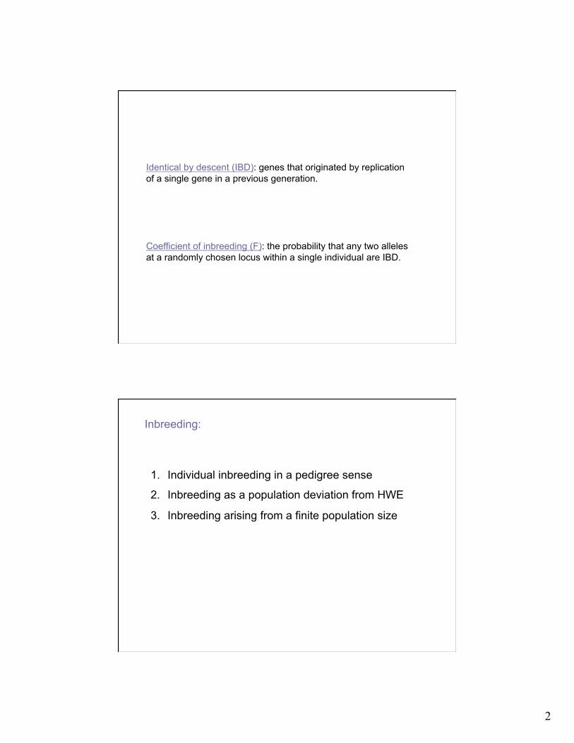
Identical by descent (IBD): genes that originated by replication of a single gene in a previous generation.
Coefficient of inbreeding (F): the probability that any two alleles at a randomly chosen locus within a single individual are IBD.
Inbreeding:
1. Individual inbreeding in a pedigree sense
2. Inbreeding as a population deviation from HWE
3. Inbreeding arising from a finite population size
3
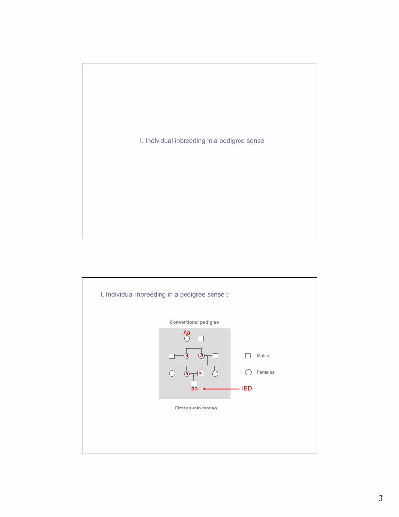
I. Individual inbreeding in a pedigree sense
I. Individual inbreeding in a pedigree sense :
Conventional pedigree
Males
Females
First cousin mating
Aa
a
a a
a
aa IBD
4
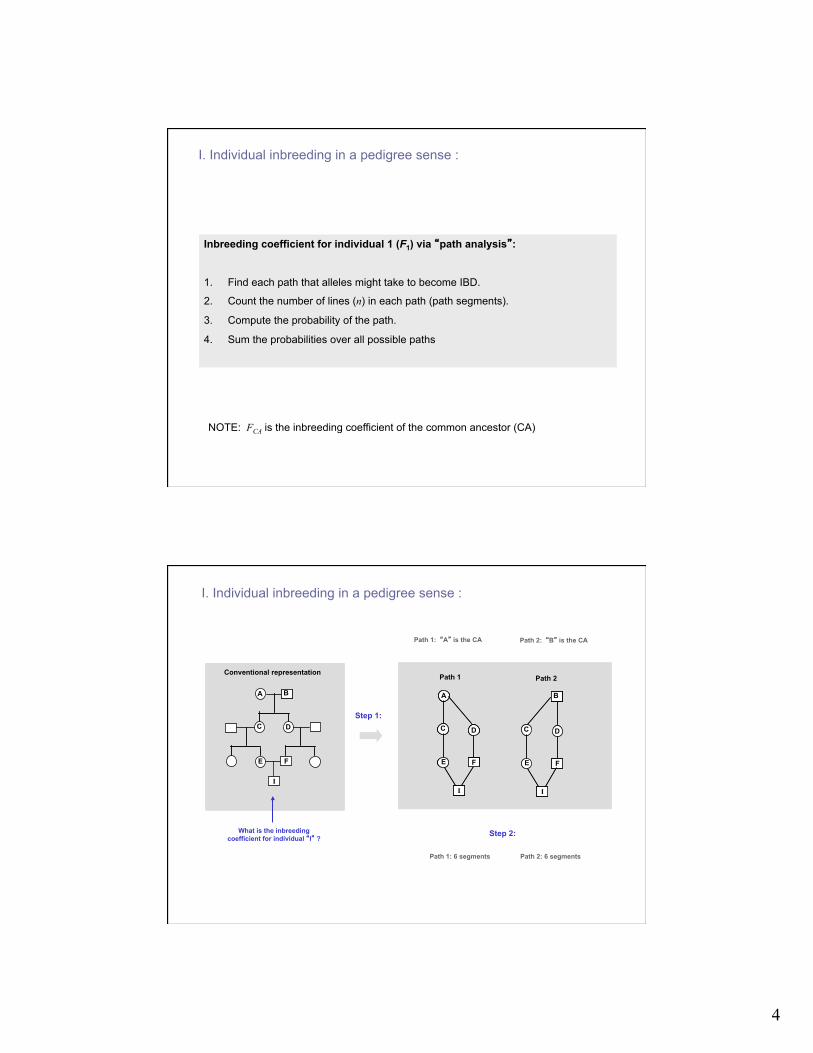
Inbreeding coefficient for individual 1 (F1) via “path analysis”:
1. Find each path that alleles might take to become IBD.
2. Count the number of lines (n) in each path (path segments).
3. Compute the probability of the path.
4. Sum the probabilities over all possible paths
I. Individual inbreeding in a pedigree sense :
NOTE: FCA is the inbreeding coefficient of the common ancestor (CA)
A B
C D
E F
I
Conventional representation
A BB
C D
E F
I
Conventional representation
A
C D
E F
I
C D
E F
I
B
Path 1 Path 2
A
C D
E F
I
AA
CC DD
EE FF
II
C D
E F
I
B
C D
E F
I
BB
Path 1 Path 2
Path 1: 6 segments Path 2: 6 segments
Path 1: “A” is the CA Path 2: “B” is the CA
What is the inbreeding coefficient for individual “I” ?
I. Individual inbreeding in a pedigree sense :
Step 1:
Step 2:
5
( )
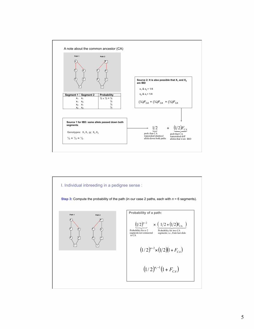
IBD that werealleles diff dtransmitte
CA that prob
pathsboth down alleleidentical transmited
CA that prob.
2121 CAF+
A note about the common ancestor (CA)
A
C D
E F I
C D
E F I
B Path 1 Path 2
Segment 1 Segment 2 Probability x1 x1 ½ × ½ = ¼ x1 x2 ¼ x2 x1 ¼ x2 x2 ¼
Genotypes: X1 X1 or X2 X2
¼ + ¼ = ½
Source 1 for IBD: same allele passed down both segments
Source 2: It is also possible that X1 and X2 are IBD
(¼)FCA + (¼)FCA = (½)FCA
x1 & x2 = 1/4
x2 & x1= 1/4
I. Individual inbreeding in a pedigree sense : Step 3: Compute the probability of the path (in our case 2 paths, each with n = 6 segments).
A
C D
E F I
C D
E F I
B Path 1 Path 2
( ) ( )CAn Fi +− 12/1 1
Probability of a path:
( ) ( ( ) ) slidelast from i.e., segments;
CA for twoy Probabilit
CA
CA toconnectednot segments
2-nfor y Probabilit
2 F2121 21 +×−n
( ) ( )( )CAn F+×− 1212/1 2
6
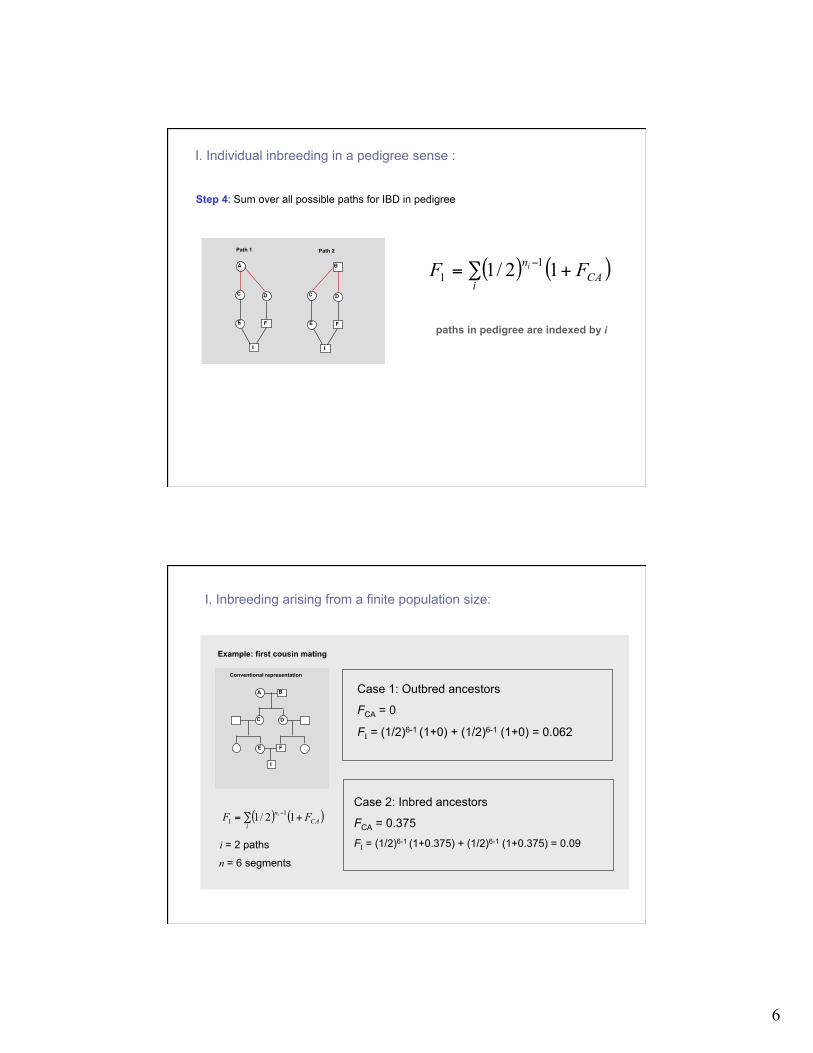
( ) ( )CAn
iFF i +∑= − 12/1 1
1
Step 4: Sum over all possible paths for IBD in pedigree
I. Individual inbreeding in a pedigree sense :
paths in pedigree are indexed by i
A
C D
E F I
C D
E F I
B Path 1 Path 2
I. Inbreeding arising from a finite population size:
Example: first cousin mating
A B
C D
E F I
Conventional representation
( ) ( )CAn
iFF i +∑= − 12/1 1
I
i = 2 paths
n = 6 segments
Case 1: Outbred ancestors
FCA = 0
FI = (1/2)6-1 (1+0) + (1/2)6-1 (1+0) = 0.062
Case 2: Inbred ancestors
FCA = 0.375 FI = (1/2)6-1 (1+0.375) + (1/2)6-1 (1+0.375) = 0.09
7
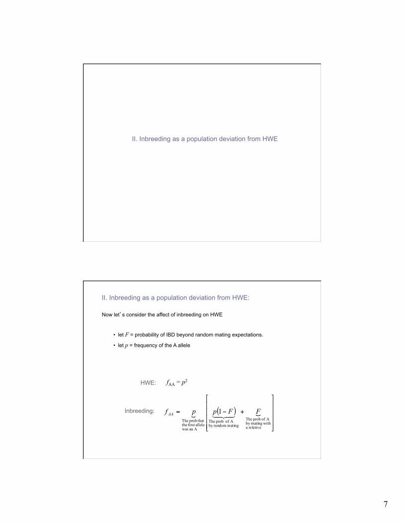
II. Inbreeding as a population deviation from HWE
II. Inbreeding as a population deviation from HWE: Now let’s consider the affect of inbreeding on HWE
• let F = probability of IBD beyond random mating expectations.
• let p = frequency of the A allele
( )
⎥⎥⎥⎥
⎦
⎤
⎢⎢⎢⎢
⎣
⎡
+−=
relative a withmatingby
A of prob Themating randomby
A of prob The
Aan was allelefirst the
thatprob The
1 FFppf AA
fAA = p2 HWE:
Inbreeding:
8
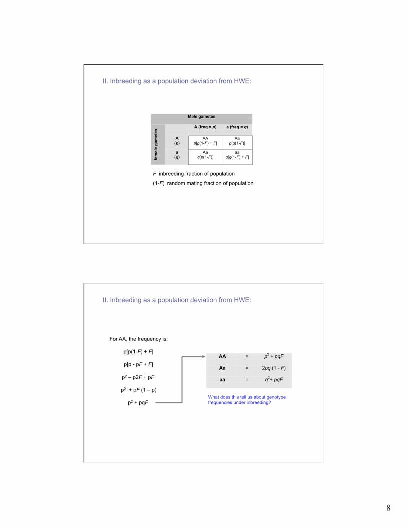
II. Inbreeding as a population deviation from HWE:
Male gametes
A (freq = p) a (freq = q)
A (p)
AA p[p(1-F) + F]
Aa p[q(1-F)]
fem
ale
gam
etes
a
(q) Aa
q[p(1-F)] aa
q[q(1-F) + F]
F inbreeding fraction of population
(1-F) random mating fraction of population
II. Inbreeding as a population deviation from HWE:
For AA, the frequency is:
p[p(1-F) + F]
p[p - pF + F]
p2 – p2F + pF
p2 + pF (1 – p)
p2 + pqF
AA = p2 + pqF
Aa = 2pq (1 - F)
aa = q2+ pqF
What does this tell us about genotype frequencies under inbreeding?
9
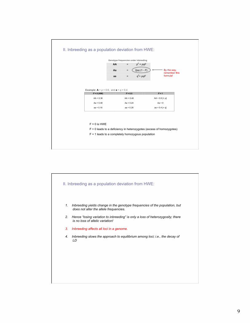
II. Inbreeding as a population deviation from HWE:
F = 0 (HW) F = 0.5 F = 1
AA = 0.36
AA = 0.48
AA = 0.6 [= p]
Aa = 0.48
Aa = 0.24
Aa = 0
aa = 0.16
aa = 0.28
aa = 0.4 [= q]
AA = p2 + pqF
Aa = 2pq (1 - F)
aa = q2+ pqF
Genotype frequencies under inbreeding
Example: A = p = 0.6, and a = q = 0.4
F = 0 is HWE
F > 0 leads to a deficiency in heterozygotes (excess of homozygotes)
F = 1 leads to a completely homozygous population
By the way, remember this formula!
II. Inbreeding as a population deviation from HWE:
1. Inbreeding yields change in the genotype frequencies of the population, but does not alter the allele frequencies.
2. Hence “losing variation to inbreeding” is only a loss of heterozygosity; there is no loss of allelic variation!
3. Inbreeding affects all loci in a genome.
4. Inbreeding slows the approach to equilibrium among loci; i.e., the decay of LD
10
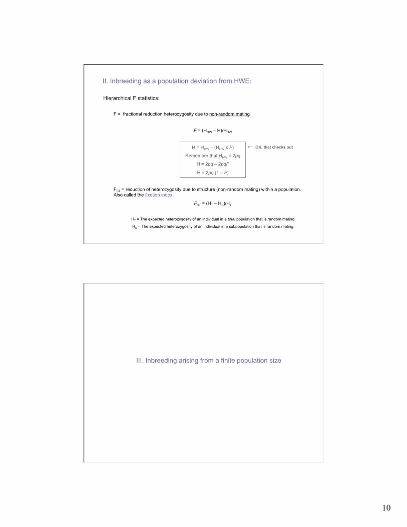
II. Inbreeding as a population deviation from HWE: Hierarchical F statistics:
F = fractional reduction heterozygosity due to non-random mating
F = (HHW – H)/HHW
H = HHW – (HHW x F)
Remember that HHW = 2pq
H = 2pq – 2pqF
H = 2pq (1 – F)
FST = reduction of heterozygosity due to structure (non-random mating) within a population. Also called the fixation index.
FST = (HT – HS)/HT
HT = The expected heterozygosity of an individual in a total population that is random mating
HS = The expected heterozygosity of an individual in a subpopulation that is random mating
OK, that checks out
III. Inbreeding arising from a finite population size
11
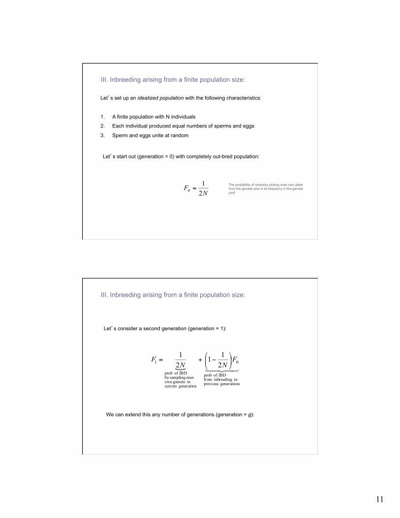
III. Inbreeding arising from a finite population size: Let’s set up an idealized population with the following characteristics:
1. A finite population with N individuals
2. Each individual produced equal numbers of sperms and eggs
3. Sperm and eggs unite at random
Let’s start out (generation = 0) with completely out-bred population:
NF
21
0 =The probability of randomly picking ones own allele from the gamete pool is its frequency in the gamete pool
III. Inbreeding arising from a finite population size:
sgeneration previousin inbreeding from
IBD of prob
0
generationcurrent in gameteown ones samplingby
IBD of prob
1 211
21 F
NNF ⎟
⎠
⎞⎜⎝
⎛ −+=
Let’s consider a second generation (generation = 1):
We can extend this any number of generations (generation = g):
12
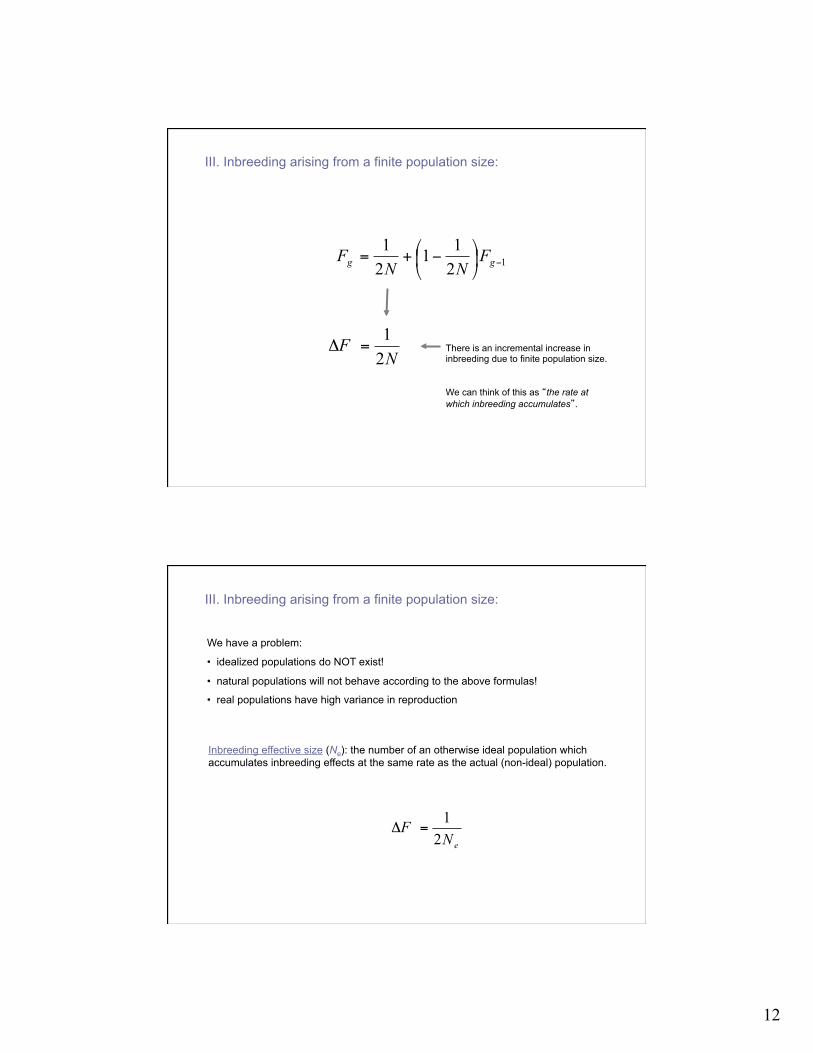
III. Inbreeding arising from a finite population size:
NF
21
=Δ
1211
21
−⎟⎠
⎞⎜⎝
⎛ −+= gg FNN
F
There is an incremental increase in inbreeding due to finite population size.
We can think of this as “the rate at which inbreeding accumulates”.
III. Inbreeding arising from a finite population size:
We have a problem:
• idealized populations do NOT exist!
• natural populations will not behave according to the above formulas!
• real populations have high variance in reproduction
eNF
21
=Δ
Inbreeding effective size (Ne): the number of an otherwise ideal population which accumulates inbreeding effects at the same rate as the actual (non-ideal) population.
13
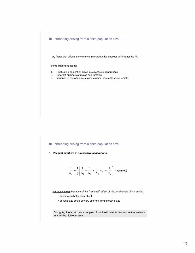
III. Inbreeding arising from a finite population size:
Any factor that affects the variance in reproductive success will impact the Ne Some important cases: 1. Fluctuating population sizes in successive generations 2. Different numbers of males and females 3. Variance in reproductive success (other than male verse female)
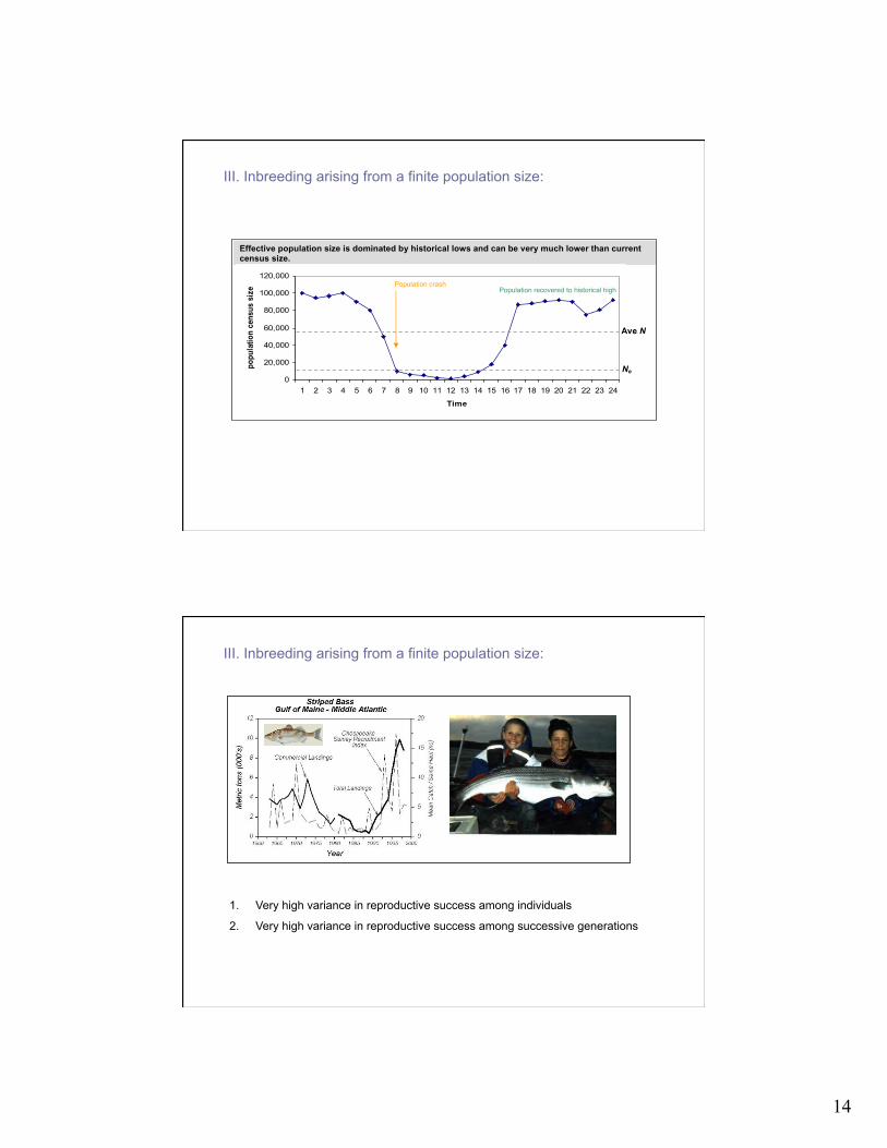
III. Inbreeding arising from a finite population size: 1. Unequal numbers in successive generations
(approx.) 1...11111
321 ⎥⎥⎦
⎤
⎢⎢⎣
⎡++++=
ge NNNNgN
Harmonic mean because of the “residual” effect of historical levels of inbreeding
• sensitive to bottleneck effect
• census size could be very different from effective size
Droughts, floods, etc. are examples of stochastic events that ensure the variance in N will be high over time
14
III. Inbreeding arising from a finite population size:
Effective population size is dominated by historical lows and can be very much lower than current census size.
0
20,000
40,000
60,000
80,000
100,000
120,000
1 2 3 4 5 6 7 8 9 10 11 12 13 14 15 16 17 18 19 20 21 22 23 24
Time
popu
latio
n ce
nsus
siz
e
Ave N
Ne
Population crash Population recovered to historical high
III. Inbreeding arising from a finite population size:
1. Very high variance in reproductive success among individuals
2. Very high variance in reproductive success among successive generations
15
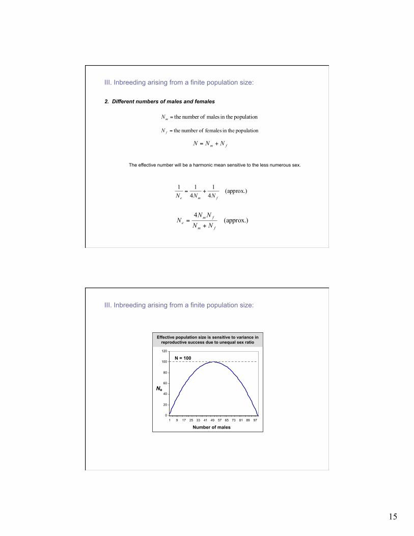
III. Inbreeding arising from a finite population size: 2. Different numbers of males and females
population in the males ofnumber the=mN
population in the females ofnumber the=fN
fm NNN +=
(approx.) 4
14
11
fme NNN+=
(approx.) 4
fm
fme NN
NNN
+=
The effective number will be a harmonic mean sensitive to the less numerous sex.
III. Inbreeding arising from a finite population size:
0
20
40
60
80
100
120
1 9 17 25 33 41 49 57 65 73 81 89 97
Number of males
Ne
N = 100
Effective population size is sensitive to variance in reproductive success due to unequal sex ratio
16
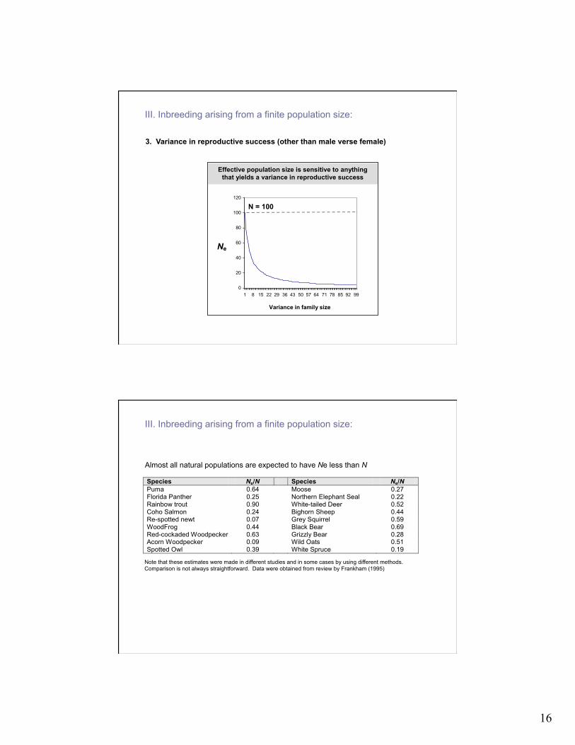
III. Inbreeding arising from a finite population size: 3. Variance in reproductive success (other than male verse female)
Variance in family size
N = 100
Effective population size is sensitive to anything that yields a variance in reproductive success
0
20
40
60
80
100
120
1 8 15 22 29 36 43 50 57 64 71 78 85 92 99
N = 100
Ne
III. Inbreeding arising from a finite population size: Almost all natural populations are expected to have Ne less than N
Species Ne/N Species Ne/N Puma 0.64 Moose 0.27 Florida Panther 0.25 Northern Elephant Seal 0.22 Rainbow trout 0.90 White-tailed Deer 0.52 Coho Salmon 0.24 Bighorn Sheep 0.44 Re-spotted newt 0.07 Grey Squirrel 0.59 WoodFrog 0.44 Black Bear 0.69 Red-cockaded Woodpecker 0.63 Grizzly Bear 0.28 Acorn Woodpecker 0.09 Wild Oats 0.51 Spotted Owl 0.39 White Spruce 0.19
Note that these estimates were made in different studies and in some cases by using different methods. Comparison is not always straightforward. Data were obtained from review by Frankham (1995)
17
Inbreeding depression: the decrease in the mean fitness of individuals arising from a greater frequency of the homozygous recessive genotypes for deleterious alleles, as compared with outbred individuals
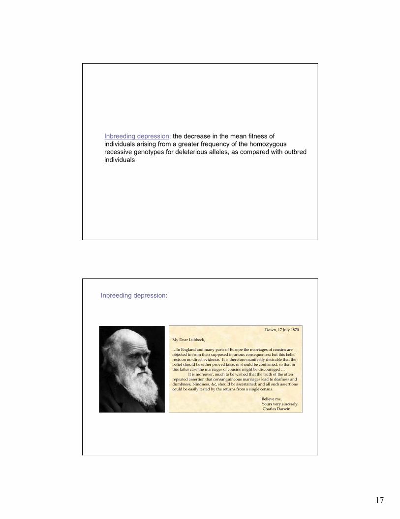
Inbreeding depression:
Down, 17 July 1870
My Dear Lubbock, …In England and many parts of Europe the marriages of cousins are objected to from their supposed injurious consequences: but this belief rests on no direct evidence. It is therefore manifestly desirable that the belief should be either proved false, or should be confirmed, so that in this latter case the marriages of cousins might be discouraged … It is moreover, much to be wished that the truth of the often repeated assertion that consanguineous marriages lead to deafness and dumbness, blindness, &c, should be ascertained: and all such assertions could be easily tested by the returns from a single census. Believe me, Yours very sincerely, Charles Darwin
18
Inbreeding depression:
Let’s use our knowledge of populating genetics to determine if inbreeding will lead to an increased chance of the CF allele appearing as a homozygous recessive. Random mating: Frequency of CF = q = 1/2500 Risk of CF under random mating = q2 = 0.00000016 (risk projected over all genes = .4%) First cousin mating: Remember that F for the offspring of a fist cousin mating = 1/16 (assuming that the great grandparents were unrelated) Risk of CF in children of a first cousin mating = q[q(1-F) + F] = 0.00002515 (risk projected over all genes = 60%) The risk of CF in the offspring of a first cousin marriage is 157 times larger than in the offspring of a random mating.
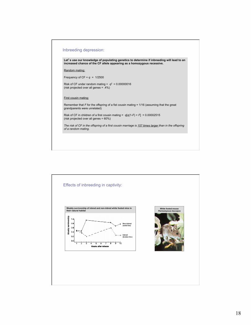
Effects of inbreeding in captivity:
Weekly survivorship of inbred and non-inbred white footed mice in their natural habitat
Non-inbred (solid line) Inbred (broken line)
White footed mouse Permomyscus leucopus
19
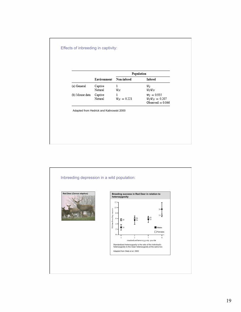
Effects of inbreeding in captivity:
Adapted from Hedrick and Kalinowski 2000
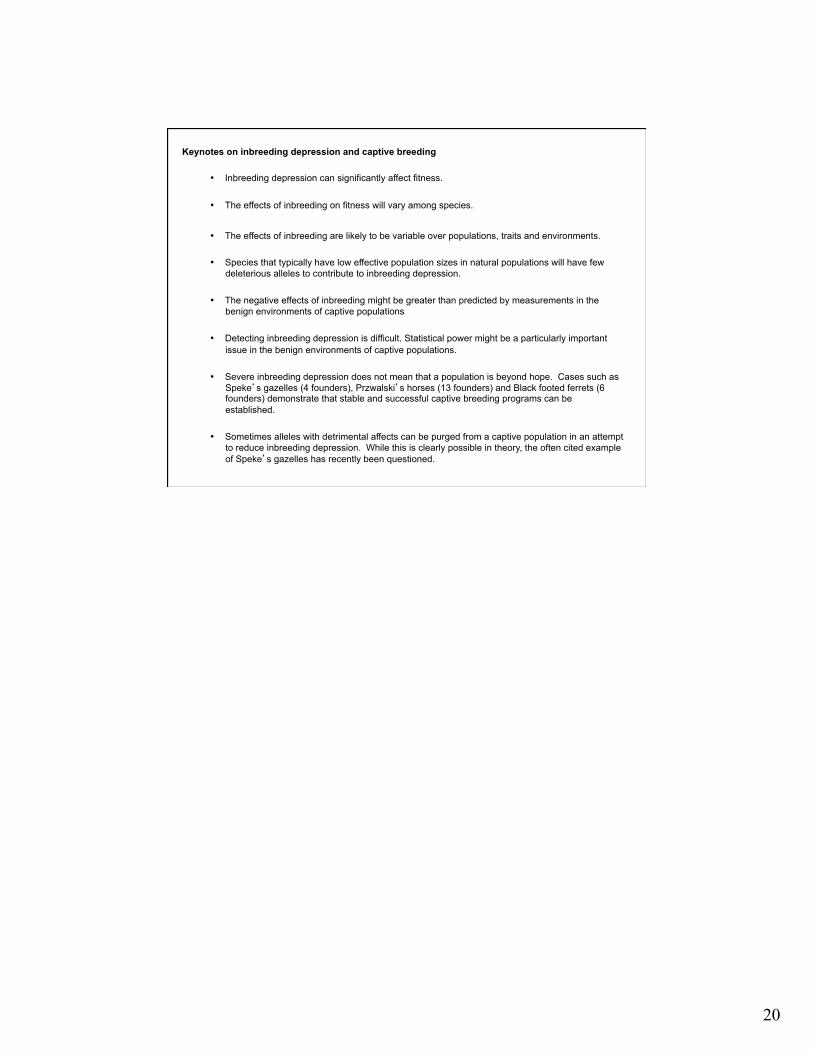
Inbreeding depression in a wild population: Red Deer (Cervus elaphus)
Males Females
Breeding success in Red Deer in relation to heterozygosity
Standardized heterozygosity is the ratio of the individual’s heterozygosity to the mean heterozygosity at the same loci. Adapted from Slate et al. 2000
20
Keynotes on inbreeding depression and captive breeding
• Inbreeding depression can significantly affect fitness.
• The effects of inbreeding on fitness will vary among species.
• The effects of inbreeding are likely to be variable over populations, traits and environments.
• Species that typically have low effective population sizes in natural populations will have few deleterious alleles to contribute to inbreeding depression.
• The negative effects of inbreeding might be greater than predicted by measurements in the
benign environments of captive populations
• Detecting inbreeding depression is difficult. Statistical power might be a particularly important issue in the benign environments of captive populations.
• Severe inbreeding depression does not mean that a population is beyond hope. Cases such as
Speke’s gazelles (4 founders), Przwalski’s horses (13 founders) and Black footed ferrets (6 founders) demonstrate that stable and successful captive breeding programs can be established.
• Sometimes alleles with detrimental affects can be purged from a captive population in an attempt
to reduce inbreeding depression. While this is clearly possible in theory, the often cited example of Speke’s gazelles has recently been questioned.
Recommended