Precourse to the PeC3 School on Numerical Modelling with Differential Equations
Precourse to the PeC3 Summer School on
Introduction on Numerical Modelling withDifferential Equations
Ole Klein1
1Universitat HeidelbergInterdisziplinares Zentrum fur Wiss. RechnenIm Neuenheimer Feld 205, D-69120 Heidelbergemail: [email protected]
Universidad Nacional Agraria La Molina,Lima, Peru, October 23–25, 2019
1 / 171

Precourse to the PeC3 School on Numerical Modelling with Differential Equations
Introduction to C++
Contents I
1 Introduction to C++
2 Best Practices for Scientific Computing
3 Floating-Point Numbers
4 Condition and Stability
5 Interpolation, Differentiation and Integration
6 Solution of Linear and Nonlinear Equations
2/ 171

Precourse to the PeC3 School on Numerical Modelling with Differential Equations
Introduction to C++
Background and First Steps
What is C++?
C++ is a programming language that was developed for bothsystem and application programming.
• Support for several programming paradigms: imperative,object oriented, generic (templates)
• Emphasizes efficiency, performance and flexibility
• Applications range from embedded controllers tohigh-performance super computers
• Allows direct management of hardware resources
• “Zero-cost abstractions”, “pay only for what you use”
• Open standard with several implementations
• Most important compilers:• Open source: GCC and Clang (LLVM)• Proprietary: Microsoft and Intel
3 / 171

Precourse to the PeC3 School on Numerical Modelling with Differential Equations
Introduction to C++
Background and First Steps
History
• 1979: Bjarne Stroustrup develops “C with Classes”
• 1985: First commercial C++ compiler
• 1989: C++ 2.0
• 1998: Standardization as ISO/IEC 14882:1998 (C++98)
• 2011: Next important version with new functionality (C++11)
• 2014: C++14 with many bug fixes and useful features
• 2017: C++17, current version
• 2020: upcoming standard
4 / 171

Precourse to the PeC3 School on Numerical Modelling with Differential Equations
Introduction to C++
Background and First Steps
First C++ Program/* make parts of the standard library available */
#include <iostream>
#include <string>
// custom function that takes a string as an argument
���� print(std::string msg)
{
// write to stdout
std::cout << msg << std::endl;
}
// main function is called at program start
��� main(��� argc, ����** argv)
{
// variable declaration and initialization
std::string greeting = "Hello, world!";
print(greeting);
������ 0;
}5 / 171

Precourse to the PeC3 School on Numerical Modelling with Differential Equations
Introduction to C++
Background and First Steps
Central Components of a C++ ProgramA basic C++ program consists of two components:
Include directives to import software libraries:• always the first lines of a program• only one include directive per line
User-defined functions:• like mathematical functions, with arguments and return value• every program must implement the function
��� main(��� argc, ����** argv)
{
...
}
This function is called by the operating system when theprogram is executed.
6 / 171

Precourse to the PeC3 School on Numerical Modelling with Differential Equations
Introduction to C++
Background and First Steps
Comments
Rules for comments in C++ code:
• Comments can be placed anywhere in the code
• Comments starting with // (C-style comments) end at a linebreak:
��� i = 42; // the answer
��� x = 0;
• Multiline comments are started by /* and ended by */:
/* This comment spans
multiple lines */
��� x = 0;
7 / 171
Precourse to the PeC3 School on Numerical Modelling with Differential Equations
Introduction to C++
Basic Building Blocks
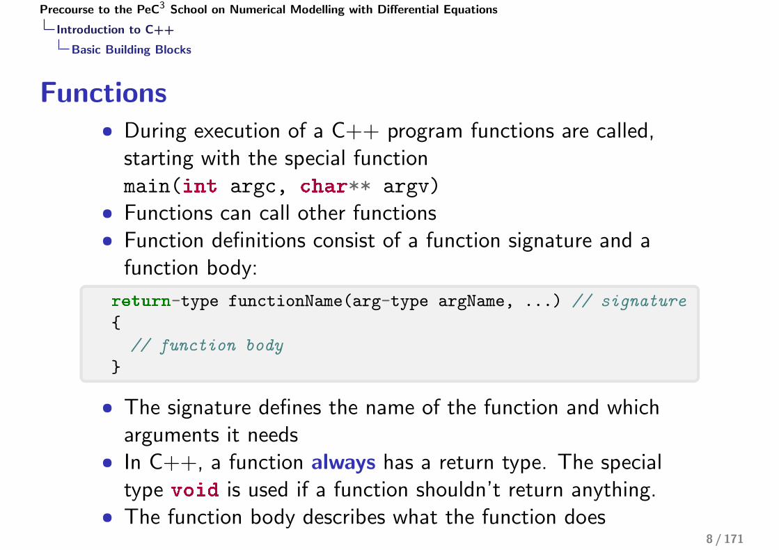
Functions• During execution of a C++ program functions are called,
starting with the special functionmain(��� argc, ����** argv)
• Functions can call other functions• Function definitions consist of a function signature and a
function body:
������-type functionName(arg-type argName, ...) // signature
{
// function body
}
• The signature defines the name of the function and whicharguments it needs
• In C++, a function always has a return type. The specialtype ���� is used if a function shouldn’t return anything.
• The function body describes what the function does8 / 171

Precourse to the PeC3 School on Numerical Modelling with Differential Equations
Introduction to C++
Basic Building Blocks
Statements
��� i = 0;
i = i + someFunction();
anotherFunction();
������ i;
i = 2; // never executed
• A C++ function consists of a number of statements, executedone by one
• Statements are separated by semicolons
• The special statement ������ val; immediately leaves thecurrent function and returns val as its return value
• ���� functions can leave out the value or even the whole������ statement
9 / 171

Precourse to the PeC3 School on Numerical Modelling with Differential Equations
Introduction to C++
Basic Building Blocks
Variables
• Variables are used for storing intermediate values
• In C++, variables always have a fixed type (integer,floating-point, text, . . . )
• Variables may contain upper and lower case letters, digits andunderscores, but may not start with a digit
• Names are case sensitive!
• Variables have to be declared before they can be used• Normal variables are declared through a statement:
variable-type variableName = initial-value;
• Function arguments are declared in the function signature:
���� func(var-type1 arg1, var-type2 arg2)
10 / 171
Precourse to the PeC3 School on Numerical Modelling with Differential Equations
Introduction to C++
Basic Building Blocks
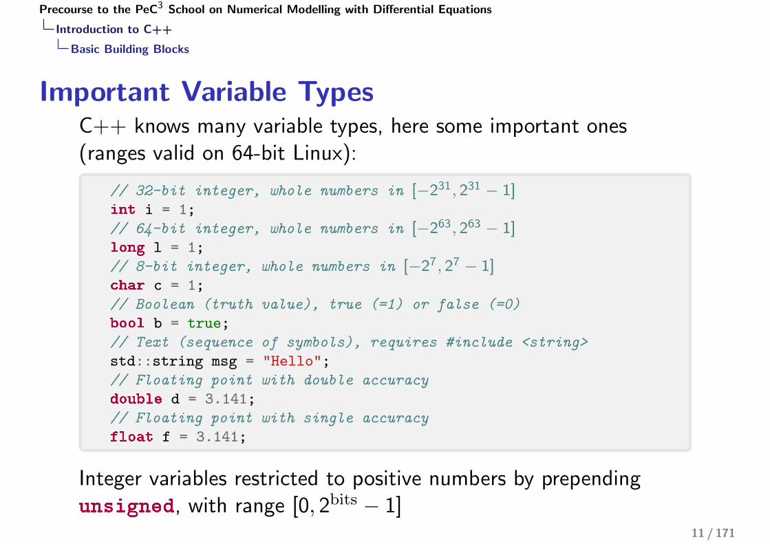
Important Variable TypesC++ knows many variable types, here some important ones(ranges valid on 64-bit Linux):
// 32-bit integer, whole numbers in [−231, 231 − 1]��� i = 1;
// 64-bit integer, whole numbers in [−263, 263 − 1]���� l = 1;
// 8-bit integer, whole numbers in [−27, 27 − 1]���� c = 1;
// Boolean (truth value), true (=1) or false (=0)
���� b = true;
// Text (sequence of symbols), requires #include <string>
std::string msg = "Hello";
// Floating point with double accuracy
������ d = 3.141;
// Floating point with single accuracy
����� f = 3.141;
Integer variables restricted to positive numbers by prepending��������, with range [0, 2bits − 1]
11 / 171

Precourse to the PeC3 School on Numerical Modelling with Differential Equations
Introduction to C++
Basic Building Blocks
Scopes and Variable Lifetime
• A block scope is a group of statements within braces (e.g.,function body)
• Scopes can be nested arbitrarily
• Variables have a limited lifetime:• the lifetime of a variable starts with its declaration• it ends when leaving the scope where it was declared
��� cube(��� x)
{
// x exists everywhere in the function
{
��� y = x * x; // y exists from here on
x = x * y;
} // here y doesn't exist anymore
������ x;
} // here x doesn't exist anymore
12 / 171

Precourse to the PeC3 School on Numerical Modelling with Differential Equations
Introduction to C++
Basic Building Blocks
Scopes and Name CollisionsIt is impossible to create two variables with the same name withina scope, and names in an inner scope temporarily shadow namesfrom an outer scope
{
��� x = 2;
��� x = 3; // compile error!
}
��� abs(��� x) { ... } // absolute value
{
��� x = -2;
{
������ x = 3.3; ��� abs = -2;
std::cout << x << std::endl; // prints 3.3
x = abs(x); // compile error, here abs is a variable!
}
x = abs(x); // now: x == 2
}
13 / 171

Precourse to the PeC3 School on Numerical Modelling with Differential Equations
Introduction to C++
Basic Building Blocks
NamespacesScopes can also have an name, and are then called namespaces.Namespaces are used to group parts of a program together thatshare functionality or form a larger unit. They are a tool for theorganization of large code bases.
��������� MyScientificProgram {
��������� LinearSolvers {
// any user-defined functions, objects, etc.,
// that deal with linear solvers
}
��������� NonlinearSolvers {
// any functions, etc., that belong to nonlinear solvers,
// e.g., Newton's method
}
}
Tools provided by the C++ standard library are in namespace std.
14 / 171

Precourse to the PeC3 School on Numerical Modelling with Differential Equations
Introduction to C++
Basic Building Blocks
ExpressionsWe use expressions to calculate things in C++
• Expressions are combinations of values, variables, functioncalls, and mathematical operators, that produce some valuethat can be assigned to a variable:
i = 2;
j = i * j;
d = std::sqrt(2.0) + j;
• Composite expressions like (a * b + c) * d use standardmathematical precedence rules, known as operatorprecedence
Rule Overview
https://en.cppreference.com/w/cpp/language/operator_
precedence
15 / 171
Precourse to the PeC3 School on Numerical Modelling with Differential Equations
Introduction to C++
Basic Building Blocks
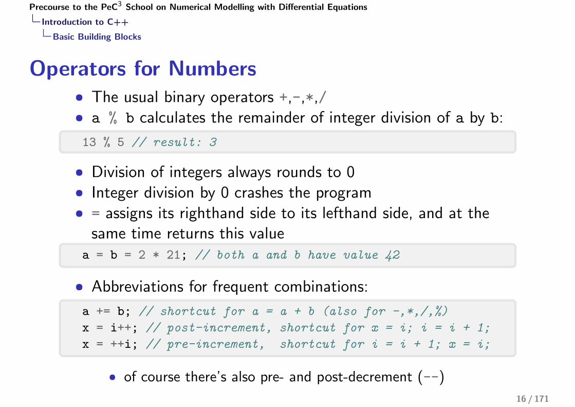
Operators for Numbers• The usual binary operators +,-,*,/• a % b calculates the remainder of integer division of a by b:
13 % 5 // result: 3
• Division of integers always rounds to 0• Integer division by 0 crashes the program• = assigns its righthand side to its lefthand side, and at the
same time returns this valuea = b = 2 * 21; // both a and b have value 42
• Abbreviations for frequent combinations:
a += b; // shortcut for a = a + b (also for -,*,/,%)
x = i++; // post-increment, shortcut for x = i; i = i + 1;
x = ++i; // pre-increment, shortcut for i = i + 1; x = i;
• of course there’s also pre- and post-decrement (--)
16 / 171

Precourse to the PeC3 School on Numerical Modelling with Differential Equations
Introduction to C++
Basic Building Blocks
Comparison Operators
• Comparison operators produce truth values (����):
4 > 3; // true
• Available operators
a < b; // a strictly less than b
a > b; // a strictly greater than b
a <= b; // a less than or equal to b
a >= b; // a greater than or equal to b
a == b; // a equal to b (note the double =!)
a != b; // a not equal to b
17 / 171
Precourse to the PeC3 School on Numerical Modelling with Differential Equations
Introduction to C++
Basic Building Blocks
Combination of Truth Values
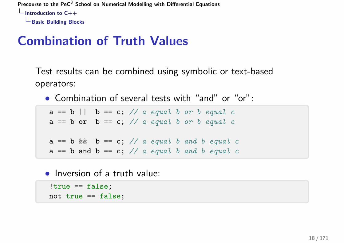
Test results can be combined using symbolic or text-basedoperators:
• Combination of several tests with “and” or “or”:
a == b || b == c; // a equal b or b equal c
a == b or b == c; // a equal b or b equal c
a == b && b == c; // a equal b and b equal c
a == b and b == c; // a equal b and b equal c
• Inversion of a truth value:!true == false;
not true == false;
18 / 171
Precourse to the PeC3 School on Numerical Modelling with Differential Equations
Introduction to C++
Basic Building Blocks
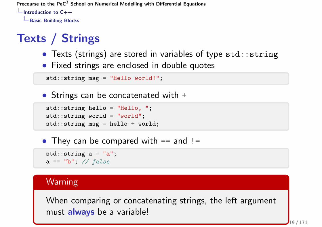
Texts / Strings• Texts (strings) are stored in variables of type std::string• Fixed strings are enclosed in double quotes
std::string msg = "Hello world!";
• Strings can be concatenated with +
std::string hello = "Hello, ";
std::string world = "world";
std::string msg = hello + world;
• They can be compared with == and !=
std::string a = "a";
a == "b"; // false
Warning
When comparing or concatenating strings, the left argumentmust always be a variable!
19 / 171

Precourse to the PeC3 School on Numerical Modelling with Differential Equations
Introduction to C++
Basic Building Blocks
Programming TasksTask 1
Consider the “hello, world!” program. Modify the programso that it uses a function mark that
• reads a std::string from std::cin
• adds an exclamation mark “!” to its end
• prints the resulting string using std::cout
Task 1
Add a function calculate that
• reads in two numbers, an ��� and a ������
• prints their sum and product on one line, separated bya space
• returns their difference as a value20 / 171

Precourse to the PeC3 School on Numerical Modelling with Differential Equations
Introduction to C++
Input and Output
I/O Streams under UNIX
• UNIX (and Linux) programs communicate with the operatingsystem using so-called I/O (Input/Output) streams
• Streams are one-way streets — you can either read from themor write to them
• Every program starts with three open streams, namely
stdin Standard input reads user input from theterminal, is connected to file descriptor 0
stdout Standard output receives results printed by theprogram, is connected to file descriptor 1
stderr Standard error output receives diagnosticmessages like errors, is connected to filedescriptor 2
21 / 171

Precourse to the PeC3 School on Numerical Modelling with Differential Equations
Introduction to C++
Input and Output
Redirecting I/O Streams I• Normally all standard streams are connected to the terminal• Sometimes it is useful to redirect these streams to files• stdout is redirected by writing "> fileName" after the
program name
[user@host ~] ls > files
[user@host ~] cat files
file1
file2
files
The output file is created before the command is executed• Error messages are still printed to the terminal
[user@host ~] ls missingdir > files
ls: missingdir: No such file or directory
[user@host ~] cat files
[user@host ~]
22 / 171

Precourse to the PeC3 School on Numerical Modelling with Differential Equations
Introduction to C++
Input and Output
Redirecting I/O Streams II
• These three operators may be combined, of course
• stdin is read from a file by appending "< fileName"
[user@host ~] cat # no argument means copying stdin to stdout
terminal input^D # (CTRL+D) terminates input
terminal input
[user@host ~] cat < files
file1
file2
files
• stderr is saved to file by using "2> fileName"
[user@host ~] ls missingdir 2> error
[user@host ~] cat error
ls: missingdir: No such file or directory
• These three operators may be combined, of course
23 / 171

Precourse to the PeC3 School on Numerical Modelling with Differential Equations
Introduction to C++
Input and Output
Printing to the Terminal
• A C++ program can use the three streams stdin, stdout andstderr to communicate with a user on the terminal (shell)
• Output uses std::cout. Everything we want to print is“pushed” into the standard output using <<
#include <iostream> // required for input / output
...
std::string user = "Joe";
std::cout << "Hello, " << user << std::endl;
• A line break is created by printing std::endl (end line)
24 / 171

Precourse to the PeC3 School on Numerical Modelling with Differential Equations
Introduction to C++
Input and Output
Reading from the Terminal
• Reading user input uses std::cin
• The corresponding variable has to be created first
• Input is “pulled” out of standard input with >>
#include <iostream>
...
std::string user = "";
��� answer = 0;
std::cout << "Enter your name: " << std::endl;
std::cin >> user;
std::cout << "Enter your answer: " << std::endl;
std::cin >> answer;
std::cout << "Hi " << user << "! Your answer was: "
<< answer << std::endl;
• Input on the terminal has to be committed using the returnkey
25 / 171

Precourse to the PeC3 School on Numerical Modelling with Differential Equations
Introduction to C++
Control Flow
Control Flow
Most programs are impossible or very difficult to write as a simplesequence of statements in fixed order.
Examples:
• a function returning the absolute value of a number
• a function catching division by zero and printing an errormessage
• a function summing all numbers from 1 to N ∈ N• . . .
Programming languages contain special statements that executedifferent code paths based on the value of an expression
26 / 171

Precourse to the PeC3 School on Numerical Modelling with Differential Equations
Introduction to C++
Control Flow
Branches• The �� statement executes different code depending on
whether an expression is true or false
��� abs(��� x)
{
�� (x > 0)
{
������ x;
}
����
{
������ -x;
}
}
• The ���� clause is optional:
�� (weekday == "Wednesday")
{
cpp_lecture();
}
27 / 171

Precourse to the PeC3 School on Numerical Modelling with Differential Equations
Introduction to C++
Control Flow
Repetition
Often, a program has to execute the same code several times, e.g.,when calculating the sum
�ni=1 i
Two different approaches:
• Recursion: the function calls itself with different arguments
• Iteration: a special statement executes a list of statementsseveral times
28 / 171

Precourse to the PeC3 School on Numerical Modelling with Differential Equations
Introduction to C++
Control Flow
Recursion• Idea: a function calls itself again and again with changed
input arguments, until some termination criterion is fulfilled:
��� sum_recursive(��� n)
{
�� (n > 0)
{
������ sum_recursive(n - 1) + n;
}
����
{
������ 0;
}
}
• Requires at least one �� statement, with exactly one of thebranches calling the function again!
• Not suitable for functions that don’t return anything and onlyhave side effects (e.g., printing the first N numbers on theterminal) 29 / 171
Precourse to the PeC3 School on Numerical Modelling with Differential Equations
Introduction to C++
Control Flow
Recursion: Example
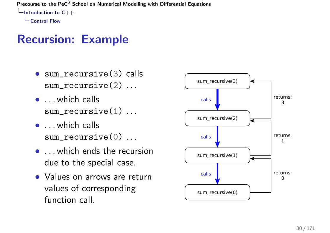
• sum_recursive(3) callssum_recursive(2) . . .
• . . . which callssum_recursive(1) . . .
• . . . which callssum_recursive(0) . . .
• . . . which ends the recursiondue to the special case.
• Values on arrows are returnvalues of correspondingfunction call.
30 / 171

Precourse to the PeC3 School on Numerical Modelling with Differential Equations
Introduction to C++
Control Flow
Iteration Using While Loop
• A ����� loop executes the following block repeatedly, as longas its expression evaluates as true
��� sum_iterative(��� n)
{
��� result = 0;
��� i = 0;
����� (i <= n)
{
result += i;
++i;
}
������ result;
}
• Often easier to understand
• Often more explicit and requires more variables
31 / 171

Precourse to the PeC3 School on Numerical Modelling with Differential Equations
Introduction to C++
Control Flow
Iteration with For Loop I
• Many loops are executed several times for different values ofsome counting variable (index)
• C++ has a special ��� loop for these cases:
��� sum_for(��� n)
{
��� result = 0;
��� (��� i = 0 ; i <= n ; ++i)
{
result += i;
}
������ result;
}
• communicates to the reader that we sum over some index
• restricts lifetime of i to the loop itself
• somewhat more complicated than a ����� loop
32 / 171

Precourse to the PeC3 School on Numerical Modelling with Differential Equations
Introduction to C++
Control Flow
Iteration with For Loop II
Every ��� loop can be converted into an equivalent ����� loop:
��� (��� i = 0 ; i <= n ; ++i)
{
...
}
becomes
{
��� i = 0;
����� (i <= n)
{
... ;
++i;
}
}
33 / 171

Precourse to the PeC3 School on Numerical Modelling with Differential Equations
Introduction to C++
Control Flow
Integer PowersConsider q ∈ N raised to the power of n ∈ N.
Recursive definition:
qn :=
�qn−1 · q if n > 0
1 if n = 0
“Iterative definition”:
qn := q · · · · · q� �� �n times
Task
How can this function be implemented in C++?
34 / 171
Precourse to the PeC3 School on Numerical Modelling with Differential Equations
Introduction to C++
Control Flow
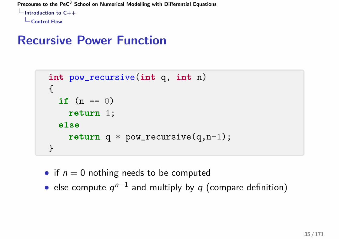
Recursive Power Function
��� pow_recursive(��� q, ��� n)
{
�� (n == 0)
������ 1;
����
������ q * pow_recursive(q,n-1);
}
• if n = 0 nothing needs to be computed
• else compute qn−1 and multiply by q (compare definition)
35 / 171

Precourse to the PeC3 School on Numerical Modelling with Differential Equations
Introduction to C++
Control Flow
Iterative Power Function
��� pow_iterative(��� q, ��� n)
{
��� out = 1;
��� (��� i = 0; i < n; i++)
out *= q;
������ out;
}
• start out with value 1 (case n = 0)
• multiply with q n times
36 / 171

Precourse to the PeC3 School on Numerical Modelling with Differential Equations
Introduction to C++
Control Flow
Recursive Power Function II��� pow_rec_fast(��� q, ��� n)
{
�� (n == 0)
������ 1;
����
{
��� t = pow_rec_fast(q,n/2);
�� (n % 2 == 0)
������ t*t;
����
������ q * t*t;
}
}
• qn = q2k =�qk
�2for n even
• qn = q2k+1 =�qk
�2 · q for n odd
37 / 171

Precourse to the PeC3 School on Numerical Modelling with Differential Equations
Introduction to C++
Control Flow
Iterative Power Function II
��� pow_iter_fast(��� q, ��� n)
{
��� out = 1;
����� (n > 0)
{
�� (n % 2 != 0)
{
out *= q;
n--;
}
q = q*q;
n /= 2;
}
������ out;
}
38 / 171

Precourse to the PeC3 School on Numerical Modelling with Differential Equations
Introduction to C++
Control Flow
Which Version is best?Two different measures of “best”:
Readability and conciseness: definitely the first two versions
Speed: measure time for 100 billion (108) evaluations of 230
Version Time Version Time
recursive 11.113s recursive 2 1.988siterative 7.663s iterative 2 1.397s
std::pow(): 3.378s
Note: This is the maximum range of the user-defined versions.The built-in std::pow() works for a much wider range, and alsoworks for floating-point arguments. This explains why it is moreexpensive.
39 / 171

Precourse to the PeC3 School on Numerical Modelling with Differential Equations
Introduction to C++
Control Flow
Which Version is best? IIThese results were obtained without optimization. Compilers canoptimize code and produce equivalent programs that aresignificantly faster (e.g., compiler option -O2).
What changes when we turn on optimization?
Version Time Version Time
recursive 0.001s recursive 2 1.317siterative 0.001s iterative 2 0.257s
std::pow(): 0.001s
The simplest versions are now the fastest! Why? Because they aresimple enough to be optimized away (evaluated at compile time)
Therefore: don’t think too much about optimal code, most of thetime it is irrelevant, and if not, measure
40 / 171

Precourse to the PeC3 School on Numerical Modelling with Differential Equations
Introduction to C++
Classes and Templates
Classes and Objects
Objects are representations of components of a program, i.e., aself-contained collection of data with associated functions (calledmethods).
Classes are blueprints for objects, i.e., they define how the objectsof a certain data type are structured.
Classes provide two special types of functions, constructors anddestructors, which are used to create resp. destroy objects.
41 / 171

Precourse to the PeC3 School on Numerical Modelling with Differential Equations
Introduction to C++
Classes and Templates
Example: Matrix Class
����� ������
{
�������: // can't be accessed by other parts of program
std::vector<std::vector<������> > entries; // data
��� numRows; // number of rows
��� numCols; // number of columns
������: // defines parts of object that are visible / usable
Matrix(��� numRows_, ��� numCols_); // constructor
������& elem(��� i, ��� j); // access entry
���� print(); // print to screen
��� rows(); // number of rows
��� cols(); // number of columns
};
42 / 171

Precourse to the PeC3 School on Numerical Modelling with Differential Equations
Introduction to C++
Classes and Templates
Encapsulation
����� ������
{
������:
// a list of public methods
�������:
// a list of private methods and attributes
};
The keyword ������: marks the description of the interface, i.e.,those methods of the class which can be accessed from the outside.
The keyword �������: accompanies the definition of attributesand methods that are only available to objects of the same class.This includes the data and implementation-specific methodsreqired by the class. To ensure data integrity it should not bepossible to access stored data from outside the class.
43 / 171

Precourse to the PeC3 School on Numerical Modelling with Differential Equations
Introduction to C++
Classes and Templates
Definition of Methods
����� ������
{
������:
// ...
������& elem(��� i, ��� j)
{
������ entries[i][j];
}
};
The method definition (i.e., listing of the actual function code) canbe placed directly in the class (so-called inline functions). In thecase of inline functions the compiler can omit the function call anduse the code directly.
44 / 171

Precourse to the PeC3 School on Numerical Modelling with Differential Equations
Introduction to C++
Classes and Templates
Definition of Methods II
���� Matrix::Matrix(��� numRows_, ��� numCols_)
{
entries.resize(numRows_);
��� (��� i = 0; i < entries.size(); i++)
entries[i].resize(numCols_);
numRows = numRows_;
numCols = numCols_;
}
If methods are defined outside the definition of a class, then thename of the method must be prefixed with the name of the classfollowed by two colons.
45 / 171

Precourse to the PeC3 School on Numerical Modelling with Differential Equations
Introduction to C++
Classes and Templates
Generic ProgrammingOften the same algorithms are required for different types of data.Writing them again and again is tedious and error-prone.
��� square(��� x)
{
������(x*x);
}
���� square(���� x)
{
������(x*x);
}
����� square(����� x)
{
������(x*x);
}
������ square(������ x)
{
������(x*x);
}
Generic programming makes it possible to write an algorithm onceand parameterize it with the data type. The language device forthis is called �������� in C++ and can be used for functions,classes, and variables. 46 / 171

Precourse to the PeC3 School on Numerical Modelling with Differential Equations
Introduction to C++
Classes and Templates
Function Templates
A function template starts with the keyword �������� and a listof template arguments, separated by commas and enclosed byangle brackets:
��������<�������� T>
T square(T x)
{
������(x*x);
}
This way, the function basically has two types of arguments:
• Types, specified in angle brackets
• Variables, specified in parentheses
This becomes clearer when actually calling the function (seebelow).
47 / 171

Precourse to the PeC3 School on Numerical Modelling with Differential Equations
Introduction to C++
Classes and Templates
Template Instantiation
At the first use of the function with a specific combination of datatypes the compiler automatically generates code for these types.This is called template instantiation, and has to be unambiguous.
Ambiguities can be avoided through:
• Explicit type conversion of arguments
• Explicit specification of template arguments in angle brackets:
std::cout << square<���>(4) << std::endl;
The argument types must match the declaration and the typeshave to provide all the necessary operations (e.g. the��������*()).
48 / 171
Precourse to the PeC3 School on Numerical Modelling with Differential Equations
Introduction to C++
Classes and Templates
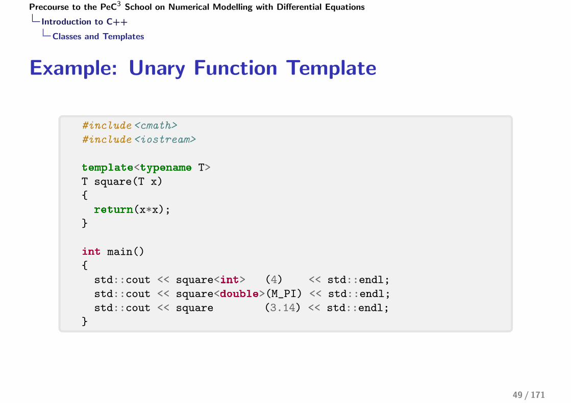
Example: Unary Function Template
#include <cmath>
#include <iostream>
��������<�������� T>
T square(T x)
{
������(x*x);
}
��� main()
{
std::cout << square<���> (4) << std::endl;
std::cout << square<������>(M_PI) << std::endl;
std::cout << square (3.14) << std::endl;
}
49 / 171

Precourse to the PeC3 School on Numerical Modelling with Differential Equations
Introduction to C++
Classes and Templates
Example: Binary Function Template#include <iostream>
��������<����� �>
����� U& maximum(����� U& a, ����� U& b)
{
�� (a > b)
������ a;
����
������ b;
}
��� main()
{
std::cout << maximum(1,4) << std::endl;
std::cout << maximum(3.14,7.) << std::endl;
std::cout << maximum(6.1,4) << std::endl; // comp. error
std::cout << maximum<������>(6.1,4) << std::endl; // unambiguous
std::cout << maximum(6.1,������(4)) << std::endl; // unambiguous
std::cout << maximum<���>(6.1,4) << std::endl; // warning
}
50 / 171

Precourse to the PeC3 School on Numerical Modelling with Differential Equations
Introduction to C++
Classes and Templates
Specialization of Function Templates
It is possible to define special template functions for certainparameter values. This is called template specialization. It can,e.g., be used for speed optimizations:
�������� <�������� V, ������ N>
������ scalarProduct(����� V& a, ����� V& b)
{
������ result = 0;
��� (������ i = 0; i < N; ++i)
result += a[i] * b[i];
������ result;
};
��������<�������� V>
������ scalarProduct<V,2>(����� V& a, ����� V& b)
{
������ a[0] * b[0] + a[1] * b[1];
};
51 / 171

Precourse to the PeC3 School on Numerical Modelling with Differential Equations
Introduction to C++
Classes and Templates
Class TemplatesIn addition to function templates, it is often also useful toparameterize classes. Here is a simple stack as an example:
��������<�������� T>
����� �����
{
�������:
std::vector<T> elems; // storage for elements of type T
������:
���� push(����� T&); // put new element on top of storage
���� pop(); // retrieve uppermost element
T top() �����; // look at uppermost element
���� empty() ����� // check if stack is empty
{
������ elems.empty();
}
};
// + implementations of push, pop, and top
52 / 171

Precourse to the PeC3 School on Numerical Modelling with Differential Equations
Introduction to C++
Classes and Templates
Further Reading
Online Tutorials
http://www.cplusplus.com/doc/tutorial/
Quick Reference
https://en.cppreference.com/w/
Other Resources
https://isocpp.org/get-started/
53 / 171

Precourse to the PeC3 School on Numerical Modelling with Differential Equations
Best Practices for Scientific Computing
Best Practices for Scientific ComputingG. Wilson, D.A. Aruliah, C.T. Brown, N.P.C. Hong, M. Davis,R.T. Guy, S.H.D. Haddock, K.D. Huff, I.M. Mitchell,M.D. Plumbley, B. Waugh, E.P. White, P. Wilson:Best Practices for Scientific Computing, PLOS Biology
1 Write programs for people, not computers
2 Let the computer do the work
3 Make incremental changes
4 Don’t repeat yourself (or others)
5 Plan for mistakes
6 Optimize software only after it works correctly
7 Document design and purpose, not mechanics
8 Collaborate
54 / 171

Precourse to the PeC3 School on Numerical Modelling with Differential Equations
Best Practices for Scientific Computing
Write Programs for People, not Computers
Software must be easy to read and understand by otherprogrammers (especially your future self!)
• Programs should not require readers to hold more than ahandful of facts in memory at once
• Short-term memory: The Magical Number Seven, Plus orMinus Two
• Chunking (psychology): binding individual pieces ofinformation into meaningful whole
• Good reason for encapsulation and modularity
• Make names and identifiers consistent, distinctive, andmeaningful
• Make coding style and formatting consistent
55 / 171

Precourse to the PeC3 School on Numerical Modelling with Differential Equations
Best Practices for Scientific Computing
Minimum Style RequirementsProgramming style conventions can be inconvenient, but there is abare minimum that should be followed in any case:
• Properly indent your code, use meaningful names for variablesand functions
• Comment your code, but don’t comment every line: mainidea/purpose of class or function, hidden assumptions, criticaldetails
• Don’t just fix compilation errors, also make sure that thecompiler doesn’t issue warnings
This makes it easier for other people to understand your work,including:
• Colleagues you may ask for help or input• Other researchers extending or using your work• Yourself in a few weeks or months (!)
56 / 171
Precourse to the PeC3 School on Numerical Modelling with Differential Equations
Best Practices for Scientific Computing
Let the Computer do the Work1
Typing the same commands over and over again is bothtime-consuming and error-prone
• Make the computer repeat tasks (i.e., write shell scripts orpython scripts)
• Save recent commands in a file for re-use (actually, that’salready done for you, search for “reverse-i-search” online)
• Use a build tool to automate workflows (e.g., makefiles,cmake)
But make sure you don’t waste time building unnecessarilyintricate automation structures!
1italics: my personal remarks57 / 171

Precourse to the PeC3 School on Numerical Modelling with Differential Equations
Best Practices for Scientific Computing
Make Incremental ChangesRequirements of scientific software typically aren’t known inadvance
• Work in small steps with frequent feedback and coursecorrection (e.g., agile development)
• Use a version control system (e.g., Git, GitLab)• Put everything that has been created manually under version
control• The source code, of course• Source files for papers / documents• Raw data (from field experiments or benchmarks)
Large chunks of data (data from experiments, important programresults, figures) can be stored efficiently using Git-LFS (large filestorage) extension
58 / 171

Precourse to the PeC3 School on Numerical Modelling with Differential Equations
Best Practices for Scientific Computing
Don’t Repeat Yourself (or Others)
Anything that exists in two or more places is harder to maintainand may introduce inconsistencies
• Every piece of data must have a single authoritativerepresentation in the system
• Modularize code rather than copying and pasting
• Re-use code instead of rewriting it
• Make use of external libraries (as long as it is not toocumbersome)
First point is actually known as DRY principle in general softwaredesign and engineering
59 / 171

Precourse to the PeC3 School on Numerical Modelling with Differential Equations
Best Practices for Scientific Computing
Plan for MistakesMistakes are human and happen on all levels of softwaredevelopment (e.g. bug, misconception, problematic design choice),even in experienced teams
• Add assertions to programs to check their operation• Simple form of error detection• Can serve as documentation (that is auto-updated)
• Use an off-the-shelf unit testing library• Can assist in finding unexpected side effects of code changes• In case of GitLab: GitLab CI (continuous integration)
• Turn bugs into test cases• Use a symbolic debugger (e.g. GDB, DDD, Gnome Nemiver,
LLDB)
Assertions should only be used to catch misconceptions andomissions by programmers, not expected runtime errors (file notfound, out of memory, solver didn’t converge)! 60 / 171

Precourse to the PeC3 School on Numerical Modelling with Differential Equations
Best Practices for Scientific Computing
The Importance of Backups
Losing your program code means losing months or even years ofhard work. There are three standard ways to guard against thispossibility:
• Create automatic backups (but know how the restore processworks!)
• Create a manual copy on an external drive or anothercomputer (messy!)
• Use a source code repository to manage the files
It’s a good idea to use two approaches as a precaution
Of the above options, using a repository has the largest number ofbenefits
61 / 171

Precourse to the PeC3 School on Numerical Modelling with Differential Equations
Best Practices for Scientific Computing
The Importance of Backups
Advantages of using a repository for code management:
• The repository can be on a different computer, i.e., therepository is automatically also an old-fashioned backup
• Repositories preserve project history, making it easy to retrieveolder code or compare versions
• Repositories can be shared with others for collaboration
One of the tools most often used for this is Git, which can be usedin conjunction with websites like GitHub or Bitbucket. An opensource alternative is GitLab, which can also be installed locally toprovide repositories for the research group.
62 / 171

Precourse to the PeC3 School on Numerical Modelling with Differential Equations
Best Practices for Scientific Computing
Optimize Software Only After it Works Correctly
Identifying potential bottlenecks is hard, and optimization of otherparts of the program is a waste of time
• Use a profiler to identify bottlenecks
• Write code in the highest-level language possible
This is an optimization with regard to development time
High-level prototypes (e.g. in Python, Matlab) can serve as oraclesfor low-level high-performance implementations (e.g. in C++)
63 / 171
Precourse to the PeC3 School on Numerical Modelling with Differential Equations
Best Practices for Scientific Computing
Code and Coding Efficiency
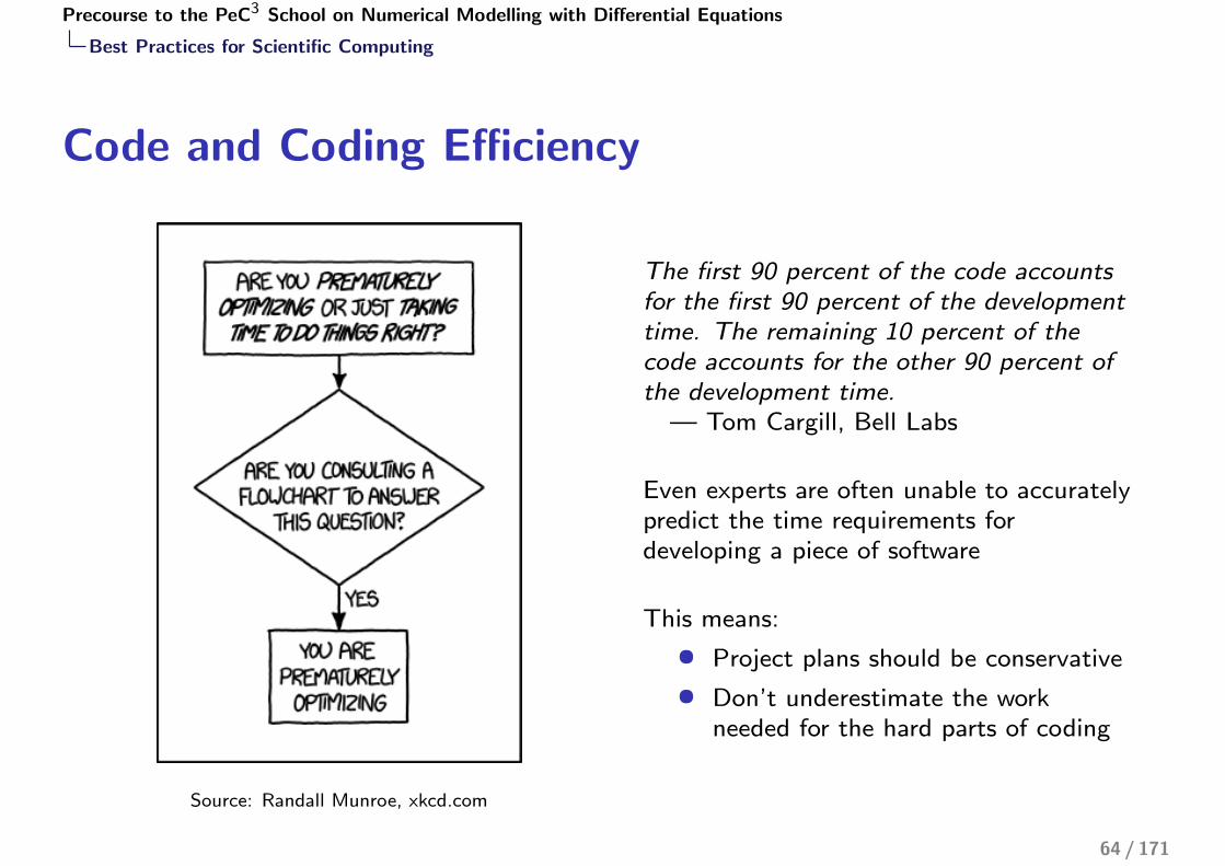
Source: Randall Munroe, xkcd.com
The first 90 percent of the code accountsfor the first 90 percent of the developmenttime. The remaining 10 percent of thecode accounts for the other 90 percent ofthe development time.
— Tom Cargill, Bell Labs
Even experts are often unable to accuratelypredict the time requirements fordeveloping a piece of software
This means:
• Project plans should be conservative
• Don’t underestimate the workneeded for the hard parts of coding
64 / 171
Precourse to the PeC3 School on Numerical Modelling with Differential Equations
Best Practices for Scientific Computing
Code and Coding Efficiency
Source: Randall Munroe, xkcd.com
Hofstadter’s Law: It always takes longerthan you expect, even when you take intoaccount Hofstadter’s Law.
— Douglas Hofstadter, Godel, Escher,Bach: An Eternal Golden Braid
As a result, there are two measures ofefficiency, the time your program needs torun, and the time you need to write it
• Don’t optimize too soon, get aworking prototype first (you willlikely need to change optimized partsalong the way)
• Look for bottlenecks and onlyoptimize those (your program willspend most of its time in roughly 5%of your code)
65 / 171

Precourse to the PeC3 School on Numerical Modelling with Differential Equations
Best Practices for Scientific Computing
Document Design and Purpose, not Mechanics
The main purpose of documentation is assistance of readers whoare trying to use an implementation, choosing between differentimplementations, or planning to extend one
• Document interfaces and reasons, not implementations• Function and method signatures• Public members of classes
• Refactor code in preference to explaining how it works
• Embed documentation for a piece of software in that software
Refactored code that needs less documentation will often save timein the long run, and documentation that is bundled with code hasmuch higher chance to stay relevant
66 / 171

Precourse to the PeC3 School on Numerical Modelling with Differential Equations
Best Practices for Scientific Computing
Collaborate
Scientific programs are often produced by research teams, and thisprovides both unique opportunities and potential sources of conflict
• Use pre-merge code reviews
• Use pair programming when bringing someone new up tospeed and when tackling particularly tricky problems
• Use an issue tracking tool
Pre-merge reviews are the only way to guarantee that code hasbeen checked by another person
Pair programming is very efficient but intrusive, and should beused with care
67 / 171

Precourse to the PeC3 School on Numerical Modelling with Differential Equations
Floating-Point Numbers
Contents I
1 Introduction to C++
2 Best Practices for Scientific Computing
3 Floating-Point Numbers
4 Condition and Stability
5 Interpolation, Differentiation and Integration
6 Solution of Linear and Nonlinear Equations
68 / 201

Precourse to the PeC3 School on Numerical Modelling with Differential Equations
Floating-Point Numbers
Representation of Numbers
Positional Notation
Definition 1 (Positional Notation)
System representing numbers x ∈ R using:
x = ± . . .m2β2 +m1β +m0 +m−1β
−1 +m−2β−2 . . .
=�
i∈Zmiβ
i
β ∈ N,β ≥ 2, is called base,mi ∈ {0, 1, 2, . . . ,β − 1} are called digits
History:
• Babylonians (≈ −1750), β = 60
• Base 10 from ∼ 1580
• Pascal: all values β ≥ 2 may be used
69 / 201
Precourse to the PeC3 School on Numerical Modelling with Differential Equations
Floating-Point Numbers
Representation of Numbers
Fixed-Point Numbers
Fixed-point numbers: truncate series after finite number of terms
x = ±n�
i=−k
miβi
Problem: scientific applications use numbers of very differentorders of magnitude
Planck constant: 6.626093 · 10−34 JsAvogadro constant: 6.021415 · 1023 1
molElectron mass: 9.109384 · 10−31 kgSpeed of light: 2.997925 · 108 m
s
Floating-point numbers can represent all such numbers withacceptable accuracy
70 / 201

Precourse to the PeC3 School on Numerical Modelling with Differential Equations
Floating-Point Numbers
Representation of Numbers
Floating-Point Numbers
Definition 2 (Floating-Point Numbers)
Let β, r , s ∈ N and β ≥ 2. The set of floating-point numbersF(β, r , s) ⊂ R consists of all numbers with the followingproperties:
1 ∀x ∈ F(β, r , s) : x = m(x) · βe(x) with
m(x) = ±r�
i=1
miβ−i , e(x) = ±
s−1�
j=0
ejβj
with digits mi and ej .m is called mantissa, e is called exponent.
2 ∀x ∈ F(β, r , s) : x = 0 ∨m1 �= 0. This is called normalizationand makes the representation unique.
71 / 201

Precourse to the PeC3 School on Numerical Modelling with Differential Equations
Floating-Point Numbers
Representation of Numbers
Example
Example 3
1 F(10, 3, 1) consists of the numbers
x = ±(m1 · 0.1 +m2 · 0.01 +m3 · 0.001) · 10±e0
with m1 �= 0 ∨ (m1 = m2 = m3 = 0), e.g., 0, 0.999 · 104, and0.123 · 10−1, but not 0.140 · 10−10 (exponent to small)
2 F(2, 2, 1) consists of the numbers
x = ±(m1 · 0.5 +m2 · 0.25) · 2±e0
=⇒ F(2, 2, 1) =�−3
2,−1,−3
4,−1
2,−3
8,−1
4, 0,
1
4,3
8,1
2,3
4, 1,
3
2
�
72 / 201
Precourse to the PeC3 School on Numerical Modelling with Differential Equations
Floating-Point Numbers
Representation of Numbers
Standard: IEEE 754 / IEC 559
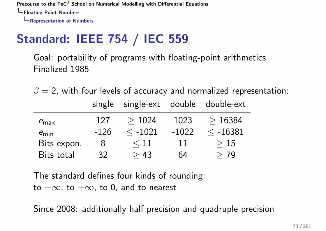
Goal: portability of programs with floating-point arithmeticsFinalized 1985
β = 2, with four levels of accuracy and normalized representation:
single single-ext double double-ext
emax 127 ≥ 1024 1023 ≥ 16384emin -126 ≤ -1021 -1022 ≤ -16381Bits expon. 8 ≤ 11 11 ≥ 15Bits total 32 ≥ 43 64 ≥ 79
The standard defines four kinds of rounding:to −∞, to +∞, to 0, and to nearest
Since 2008: additionally half precision and quadruple precision
73 / 201

Precourse to the PeC3 School on Numerical Modelling with Differential Equations
Floating-Point Numbers
Representation of Numbers
Double Precision
Let’s have a closer look at double precision:
• 64 bit in total
• 11 bit for exponent, stored without sign as c ∈ [1, 2046]
• Let e := c − 1023 =⇒ e ∈ [−1022, 1023], no sign necessary
• The values c ∈ {0, 2047} are special:• c = 0 ∧m = 0 encodes zero• c = 0 ∧m �= 0 encodes denormalized representation• c = 2047 ∧m = 0 encodes ∞ (overflow)• c = 2047 ∧m �= 0 encodes NaN = “not a number”, e.g., when
dividing by zero
74 / 201

Precourse to the PeC3 School on Numerical Modelling with Differential Equations
Floating-Point Numbers
Representation of Numbers
Double Precision
• 64− 11 = 53 bit for mantissa, one for sign,52 bit remaining for mantissa digits
• β = 2 implies m1 = 1
• This digit is called hidden bit and is never stored
• Therefore r = 53 in the sense of our definition offloating-point numbers
Double precision corresponds to F(2, 53, 10) + additional specialcodes.
75 / 201

Precourse to the PeC3 School on Numerical Modelling with Differential Equations
Floating-Point Numbers
Rounding and Rounding Error
Rounding FunctionTo approximate x ∈ R in F(β, r , s), we need a map
rd: D(β, r , s) → F(β, r , s), (1)
where D(β, r , s) ⊂ R is the domain containing F(β, r , s):
D := [X−, x−] ∪ {0} ∪ [x+,X+]
with X+/− being the numbers in F(β, r , s) with largest absolutevalue, and x+/− those with the smallest (apart from zero).
Note: this implies that x lies within the representable domain!
A reasonable demand is:
∀x ∈ D : |x − rd(x)| = miny∈F
|x − y |
(known as best approximation property)76 / 201

Precourse to the PeC3 School on Numerical Modelling with Differential Equations
Floating-Point Numbers
Rounding and Rounding Error
Rounding Function
With l(x) := max{y ∈ F|y ≤ x} and r(x) := min{y ∈ F|y ≥ x} wehave:
rd(x) =
x l(x) = r(x), x ∈ Fl(x) |x − l(x)| < |x − r(x)|r(x) |x − l(x)| > |x − r(x)|? |x − l(x)| = |x − r(x)|
The last case requires further considerations. There are severalpossible choices.
77 / 201

Precourse to the PeC3 School on Numerical Modelling with Differential Equations
Floating-Point Numbers
Rounding and Rounding Error
Natural Rounding
Definition 4 (Natural Rounding)
Let x = sign(x) ·��∞
i=1miβ−i�βe the normalized representation
of x ∈ D. Define
rd(x) :=
�l(x) = sign(x) ·
��ri=1miβ
−i�βe if 0 ≤ mr+1 < β/2
r(x) = l(x) + βe−r (last digit) ifβ/2 ≤ mr+1 < β
This is the usual rounding everyone knows from school. It has theundesirable property of introducing bias, since rounding up isslightly more likely.This is irrelevant in everyday life, but becomes important for smallβ, e.g., β = 2, and/or many operations (as in scientificcomputing).
78 / 201

Precourse to the PeC3 School on Numerical Modelling with Differential Equations
Floating-Point Numbers
Rounding and Rounding Error
Even Rounding
Definition 5 (Even Rounding)
Let (with notation as before)
rd(x) :=
l(x) if |x − l(x)| < |x − r(x)|l(x) if |x − l(x)| = |x − r(x)| ∧mr even
r(x) else
This ensures that mr in rd(x) is always even after rounding.
• For rd(x) = l(x) this is by definition.• Else rd(x) = r(x) = l(x) + βe−r , mr in l(x) is odd, and
addition of βe−r changes the last digit by one.
This choice of rounding avoids systematic drift when rounding up,and corresponds to “round to nearest” in the standard.
79 / 201

Precourse to the PeC3 School on Numerical Modelling with Differential Equations
Floating-Point Numbers
Rounding and Rounding Error
Absolute and Relative Error
Definition 6 (Absolute and Relative Error)
Let x � ∈ R an approximation of x ∈ R. Then we call
Δx := x � − x absolute error
and for x �= 0
�x � :=Δx
xrelative error
Rearranging leads to:
x � = x +Δx = x ·�1 +
Δx
x
�= x · (1 + �x �)
80 / 201

Precourse to the PeC3 School on Numerical Modelling with Differential Equations
Floating-Point Numbers
Rounding and Rounding Error
Motivation
Motivation:
Let Δx = x � − x = 100 km.For x = Distance Earth—Sun ≈ 1.5 · 108 km,
�x � =102 km
1.5 · 108 km ≈ 6.6 · 10−7
is relatively small.But for x = Distance Heidelberg—Paris ≈ 460 km,
�x � =102 km
4.6 · 102 km ≈ 0.22 (22%)
is relatively large.
81 / 201

Precourse to the PeC3 School on Numerical Modelling with Differential Equations
Floating-Point Numbers
Rounding and Rounding Error
Error Estimation
Lemma 7 (Rounding Error)
When rounding in F(β, r , 2) the absolute error fulfills
|x − rd(x)| ≤ 1
2βe(x)−r (2)
and the relative error (for x �= 0)
|x − rd(x)||x | ≤ 1
2β1−r .
This estimate is sharp (i.e., the case “=” exists).The number eps := 1
2β1−r is called machine precision.
eps = 2−24 ≈ 6 · 10−8 for single precision, andeps = 2−53 ≈ 1 · 10−16 for double precision.
82 / 201

Precourse to the PeC3 School on Numerical Modelling with Differential Equations
Floating-Point Numbers
Floating-Point Arithmetics
Floating-Point Arithmetics
We need arithmetics on F:
� : F× F → F with � ∈ {⊕,�,�,�}
corresponding to the well-known operations ∗ ∈ {+,−, ·, /} on R.
Problem: typically x , y ∈ F �=⇒ x ∗ y ∈ F
Therefore the result has to be rounded. We define
∀x , y ∈ F : x � y := rd(x ∗ y) (3)
This guarantees “exact rounding”. The implementation of such amapping is nontrivial!
83 / 201

Precourse to the PeC3 School on Numerical Modelling with Differential Equations
Floating-Point Numbers
Floating-Point Arithmetics
Guard Digit
Example 8 (Guard Digit)
Let F = F(10, 3, 1), x = 0.215 · 108, y = 0.125 · 10−5. We considerthe subtraction x � y = rd(x − y).
1 Subtraction followed by rounding requires an extreme numberof mantissa digits O(βs)!
2 Rounding before subtraction seems to produce same result.Good idea?
3 But: consider, e.g., x = 0.101 · 101, y = 0.993 · 100=⇒ relative error 18% ≈ 35 eps
4 One, two additional digits are enough to achieve exactrounding!
5 These digits are called guard digits and are also used inpractice (CPU), e.g., performing internal computations in 80bit precision.
84 / 201

Precourse to the PeC3 School on Numerical Modelling with Differential Equations
Floating-Point Numbers
Floating-Point Arithmetics
Table Maker Dilemma
Algebraic functions:e.g., polynomials, 1/x ,
√x , rational functions, . . .
more or less: finite combination of basic arithmetic operations androots
Transcendent functions:everything else, e.g., exp(x), ln(x), sin(x), xy , . . .
Table Maker Dilemma:One cannot decide a priori how many guard digits are reqired toachieve exact rounding for a given combination of transcendentfunction f and argument x .
IEEE754 guarantees exact rounding for ⊕,�,�,�, and√x .
85 / 201

Precourse to the PeC3 School on Numerical Modelling with Differential Equations
Floating-Point Numbers
Floating-Point Arithmetics
Further Problems / Properties
The following has to be considered:
• Floating-point arithmetics don’t have the associative anddistributive properties, i.e., the order of operations matters!
• There is y ∈ F, y �= 0, so that x ⊕ y = x
• Example: (�⊕ 1)� 1 = 1� 1 = 0 �= � = �⊕ 0 = �⊕ (1� 1)
• But the commutative property holds:x � y = y � x for � ∈ {⊕,�}
• Some further simple rules that are valid:• (−x)� y = −(x � y)• 1� x = x ⊕ 0 = x• x � y = 0 =⇒ x = 0 ∨ y = 0• x � z ≤ y � z if x ≤ y ∧ z > 0
86 / 201

Precourse to the PeC3 School on Numerical Modelling with Differential Equations
Condition and Stability
Contents I
1 Introduction to C++
2 Best Practices for Scientific Computing
3 Floating-Point Numbers
4 Condition and Stability
5 Interpolation, Differentiation and Integration
6 Solution of Linear and Nonlinear Equations
87 / 201

Precourse to the PeC3 School on Numerical Modelling with Differential Equations
Condition and Stability
Error Analysis
Error Analysis
Rounding errors are propagated by computations.
• Let F : Rm → Rn, in components F (x) =
F1(x1, . . . , xm)
...Fn(x1, . . . , xm)
• Compute F in a computer using numerical realizationF � : Fm → Fn.F � is an algorithm, i.e., consists of
• finitely many (= termination)• elementary (= known, i.e., ⊕,�,�,�)
operations:F �(x) = ϕl(. . .ϕ2(ϕ1(x)) . . . )
88 / 201

Precourse to the PeC3 School on Numerical Modelling with Differential Equations
Condition and Stability
Error Analysis
Error Analysis
Important:
1 A given F typically has many different realizations, because ofdifferent orders of computation
a+ b + c ≈ (a ⊕ b)⊕ c �= a⊕ (b ⊕ c)!
2 Every step ϕi contributes some (unknown) error.
3 In principle, the computational accuracy can be improvedarbitrarily, i.e., we have a sequence(F �)(k) : (F(k))
m → (F(k))n. But in the following we consider
only a given fixed finite precision.
89 / 201
Precourse to the PeC3 School on Numerical Modelling with Differential Equations
Condition and Stability
Error Analysis
Error Analysis
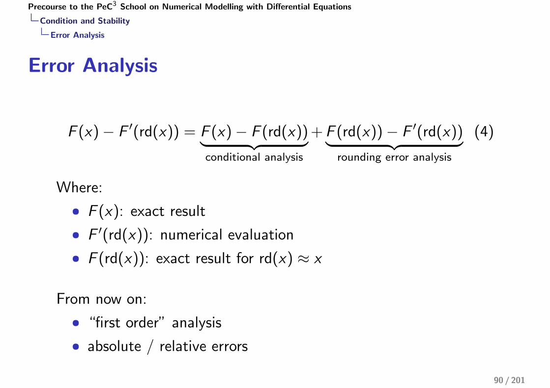
F (x)− F �(rd(x)) = F (x)− F (rd(x))� �� �conditional analysis
+F (rd(x))− F �(rd(x))� �� �rounding error analysis
(4)
Where:
• F (x): exact result
• F �(rd(x)): numerical evaluation
• F (rd(x)): exact result for rd(x) ≈ x
From now on:
• “first order” analysis
• absolute / relative errors
90 / 201

Precourse to the PeC3 School on Numerical Modelling with Differential Equations
Condition and Stability
Error Analysis
Differential Condition Analysis
We assume that F : Rm → Rn is twice continuously differentiable.Taylor’s theorem holds for the components Fi :
Fi (x +Δx) = Fi (x) +m�
j=1
∂Fi∂xj
(x)Δxj + RFi (x ;Δx) i = 1, . . . , n.
The remainder is
RFi (x ;Δx) = O
��Δx�2
�,
i.e., the approximation error is quadratic in Δx .
91 / 201

Precourse to the PeC3 School on Numerical Modelling with Differential Equations
Condition and Stability
Error Analysis
Differential Condition Analysis
Therefore, we can rearrange Taylor’s formula:
Fi (x +Δx)− Fi (x) =m�
j=1
∂Fi∂xj
(x)Δxj
� �� �leading (first) order
+RFi (x ;Δx)� �� �
higher orders
One often omits higher order terms and writes “.=” instead of “=”.
92 / 201

Precourse to the PeC3 School on Numerical Modelling with Differential Equations
Condition and Stability
Error Analysis
Differential Condition Analysis
Then we have:
Fi (x +Δx)− Fi (x)
Fi (x).=
m�
j=1
∂Fi∂xj
(x)ΔxjFi (x)
(5)
.=
m�
j=1
�∂Fi∂xj
(x)xj
Fi (x)
�
� �� �amplification factor kij (x)
·�Δxjxj
�
� �� �≤eps
,
i.e., the amplification factors kij(x) specify how (relative) input
errorsΔxjxj
contribute to (relative) errors in the i-th comp. of F !
93 / 201

Precourse to the PeC3 School on Numerical Modelling with Differential Equations
Condition and Stability
Error Analysis
Condition
Definition 9 (Condition)
We call the evaluation y = F (x) “ill-conditioned” in point x , iff|kij(x)| � 1, else “well-conditioned”.|kij(x)| < 1 is error dampening, |kij(x)| > 1 is error amplification.
The symbol “�” means “much larger than”. Normally this meansone number is several orders of magnitude larger than another(e.g., 1 million � 1).
This definition is a continuum: there is no sharp separationbetween “well-conditioned” and “ill-conditioned”!
94 / 201

Precourse to the PeC3 School on Numerical Modelling with Differential Equations
Condition and Stability
Error Analysis
Example I
Example 10
1 Addition: F (x1, x2) = x1 + x2,∂F∂x1
= ∂F∂x2
= 1.According to our formula:
F (x1 +Δx1, x2 +Δx2)− F (x1, x2)
F (x1, x2)
.= 1 · x1
x1 + x2� �� �=k1
Δx1x1
+ 1 · x2x1 + x2� �� �=k2
Δx2x2
Ill-conditioned for x1 → −x2!
95 / 201

Precourse to the PeC3 School on Numerical Modelling with Differential Equations
Condition and Stability
Error Analysis
Example II
Example 10
2 F (x1, x2) = x21 − x22 ,∂F∂x1
= 2x1,∂F∂x2
= −2x2.
F (x1 +Δx1, x2 +Δx2)− F (x1, x2)
F (x1, x2)
.= 2x1 ·
x1x21 − x22� �� �=k1
Δx1x1
+ (−2x2) ·x2
x21 − x22� �� �=k2
Δx2x2
=⇒ k1 =2x21
x21 − x22, k2 = − 2x22
x21 − x22,
Ill-conditioned for |x1| ≈ |x2|.
96 / 201

Precourse to the PeC3 School on Numerical Modelling with Differential Equations
Condition and Stability
Error Analysis
Contents I
1 Introduction to C++
2 Best Practices for Scientific Computing
3 Floating-Point Numbers
4 Condition and Stability
5 Interpolation, Differentiation and Integration
6 Solution of Linear and Nonlinear Equations
97 / 201

Precourse to the PeC3 School on Numerical Modelling with Differential Equations
Condition and Stability
Error Analysis
Rounding Error AnalysisAlso known as “forward rounding error analysis”, there are othervariants.
After error decomposition, Eq. (4):consider F (x)− F �(x) with x ∈ Fm, F � “composed” from singleoperations � ∈ {⊕,�,�,�}
Eq. (3) (exactly rounded arithmetics) and Lemma 7 (roundingerror) imply
(x � y)− (x ∗ y)(x ∗ y) = � with |�| ≤ eps
Careful, � depends on x and y , and therefore is different for eachindividual operation!
=⇒ x � y = (x ∗ y) · (1 + �) for an |�(x , y)| ≤ eps
98 / 201

Precourse to the PeC3 School on Numerical Modelling with Differential Equations
Condition and Stability
Error Analysis
Example I
Example 11
F (x1, x2) = x21 − x22 with two different realizations:
1 Fa(x1, x2) = (x1 � x1)� (x2 � x2)
2 Fb(x1, x2) = (x1 � x2)� (x1 ⊕ x2)
First realization:
u = x1 � x1 = (x1 · x1) · (1 + �1)
v = x2 � x2 = (x2 · x2) · (1 + �2)
Fa(x1, x2) = u � v = (u − v) · (1 + �3)
Fa(x1, x2)− F (x1, x2)
F (x1, x2).=
x21x21 − x22
(�1 + �3) +x22
x22 − x21(�2 + �3)
99 / 201

Precourse to the PeC3 School on Numerical Modelling with Differential Equations
Condition and Stability
Error Analysis
Example II
Example 11
Second realization:
u = x1 � x2 = (x1 − x2) · (1 + �1)
v = x1 ⊕ x2 = (x1 + x2) · (1 + �2)
Fb(x1, x2) = u � v = (u · v) · (1 + �3)
Fb(x1, x2)− F (x1, x2)
F (x1, x2).=
x21 − x22x21 − x22
(�1 + �2 + �3) = �1 + �2 + �3
=⇒ second realization is better than first realization.
100 / 201

Precourse to the PeC3 School on Numerical Modelling with Differential Equations
Condition and Stability
Error Analysis
Numerical Stability
Definition 12 (Numerical Stability)
We call a numerical algorithm “numerically stable”, if the roundingerrors accumulated during computation have the same order ofmagnitude as the unavoidable problem error from conditionanalysis.
In other words:Amplification factors from rounding analysis ≤ those fromcondition analysis =⇒ “numerically stable”
Both realizations a, b from Ex. 11 are numerically stable.
101 / 201

Precourse to the PeC3 School on Numerical Modelling with Differential Equations
Condition and Stability
Quadratic Equation
Quadratic EquationLet p2/4 > q �= 0, then the equation
y2 − py + q = 0
has two real and separate solutions
y1,2 = f±(p, q) =p
2±�
p2
4− q. (defines two f !)
Condition analysis with D :=�
p2
4 − q:
f (p +Δp, q +Δq)− f (p, q)
f (p, q)
.=
�1± p
2D
� p
p ± 2D
Δp
p− q
D (p ± 2D)
Δq
q
102 / 201

Precourse to the PeC3 School on Numerical Modelling with Differential Equations
Condition and Stability
Quadratic Equation
Quadratic EquationThis means:
• For p2
4 � q and p < 0
f−(p, q) =p
2−�
p2
4− q
is well-conditioned.
• For p2
4 � q and p > 0
f+(p, q) =p
2+
�p2
4− q
is well-conditioned.
• For p2
4 ≈ q both f+ and f− are ill-conditioned, this cannot beavoided.
103 / 201

Precourse to the PeC3 School on Numerical Modelling with Differential Equations
Condition and Stability
Quadratic Equation
Quadratic Equation
Numerically handy evaluation for the case p2
4 � q:
p < 0:
Compute y2 =p2 −
�p2
4 − q, then y1 =qy2
using Vieta’s Theorem
(q = y1 · y2).
p > 0:
Compute y1 =p2 +
�p2
4 − q, then y2 =qy1.
=⇒ every problem has to be considered individually!
104 / 201

Precourse to the PeC3 School on Numerical Modelling with Differential Equations
Condition and Stability
Cancellation
CancellationThe discussed examples contain the phenomenon of cancellation.It appears during
• addition x1 + x2 with x1 ≈ −x2• subtraction x1 − x2 with x1 ≈ x2
Remark 13Cancellation means extreme amplification of errors introducedbefore the addition or subtraction.
If x1, x2 ∈ F are machine numbers, then����(x1 � x2)− (x1 − x2)
(x1 − x2)
���� ≤ eps
holds, so this is not problematic. The problem of cancellation onlyoccurs if x1 and x2 already contain errors.
105 / 201

Precourse to the PeC3 School on Numerical Modelling with Differential Equations
Condition and Stability
Cancellation
Example
Example 14
Consider F = F(10, 4, 1).x1 = 0.11258762 · 102, x2 = 0.11244891 · 102=⇒ rd(x1) = 0.1126 · 102, rd(x2) = 0.1124 · 102
x1 − x2 = 0.13871 · 10−1, but rd(x1)− rd(x2) = 0.2 · 10−1
The result has not a single valid digit! Relative error:
0.2 · 10−1 − 0.13871 · 10−1
0.13871 · 10−1≈ 0.44 ≈ 883 · 1
2· 10−3
� �� �=eps
!
106 / 201

Precourse to the PeC3 School on Numerical Modelling with Differential Equations
Condition and Stability
Cancellation
Basic Rule
In the given example: error caused by rounding of arguments.
Source of errors is irrelevant, this also happens if x1, x2 containerrors from previous computation steps.
Rule 15Employ potentially dangerous operations as soon as possible inalgorithms, when the least possible amount of errors has beenaccumulated (compare Ex. 11).
107 / 201

Precourse to the PeC3 School on Numerical Modelling with Differential Equations
Condition and Stability
Exponential Function
Exponential FunctionThe function exp(x) = ex can be written as a power series for allx ∈ R:
exp(x) =∞�
k=0
xk
k!
Obvious approach: truncate calculation after n terms,exp(x) ≈ �n
k=0xk
k! .
Use recursion:
y0 := 1, S0 := y0 = 1,
∀k > 0: yk :=x
k· yk−1, Sk := Sk−1 + yk
yn: terms of series, Sn: partial sums
108 / 201

Precourse to the PeC3 School on Numerical Modelling with Differential Equations
Condition and Stability
Exponential Function
Error for Different Values of xResults for recursion formula with �����, n = 100:
1*10-10
1*10-5
1*100
1*105
1*1010
1*1015
1*1020
1*1025
1*1030
1*1035
1*1040
-50 -40 -30 -20 -10 0 10 20 30 40 50
relativer Fehler von exp(x)
• Negative values of x lead to arbitrarily large errors
• This effect is not caused by the truncation of the series!
109 / 201

Precourse to the PeC3 School on Numerical Modelling with Differential Equations
Condition and Stability
Exponential Function
Deviations for Imaginary Arguments
-1
-0.5
0
0.5
1
-1 -0.5 0 0.5 1
EinheitskreisAuswertung exp(z)
-2
-1.5
-1
-0.5
0
0.5
1
1.5
2
-2 -1.5 -1 -0.5 0 0.5 1 1.5 2
EinheitskreisAuswertung exp(z)
-4
-2
0
2
4
-4 -2 0 2 4
EinheitskreisAuswertung exp(z)
-10
-5
0
5
10
-10 -5 0 5 10
EinheitskreisAuswertung exp(z)
Results for the imaginary interval[−50, 50] · i
• For |z | ≤ π the result issomewhat acceptable
• For |z | → 2π the errorcontinues to grow
• Then the values leave thecircle (the trajectoryapproaches a straight lineand won’t return)
110 / 201

Precourse to the PeC3 School on Numerical Modelling with Differential Equations
Condition and Stability
Exponential Function
Visualization of Convergence Behavior
-4
-2
0
2
4
-4 -2 0 2 4
exp(2πi · 0.1)exp(2πi · 0.2)exp(2πi · 0.3)exp(2πi · 0.4)exp(2πi · 0.5)Einheitskreis
• even powers contribute tothe real part of exp(2πi · x)
• odd powers contribute tothe imaginary part
=⇒ addition of terms alternatesbetween changes to real andimaginary part
111 / 201

Precourse to the PeC3 School on Numerical Modelling with Differential Equations
Condition and Stability
Exponential Function
Visualization of Convergence Behavior
-40
-20
0
20
40
-40 -20 0 20 40
exp(2πi · 0.6)exp(2πi · 0.7)exp(2πi · 0.8)exp(2πi · 1.0)exp(2πi · 1.0)Einheitskreis
• Absolute value ofintermediate results growsexponentially in x
• Shape of trajectory looksmore and more like a square
=⇒ cancellation
112 / 201

Precourse to the PeC3 School on Numerical Modelling with Differential Equations
Condition and Stability
Exponential Function
Condition Analysis for exp(x)
For the function exp we have exp� = exp, and therefore:
exp(x +Δx)− exp(x)
exp(x).=
�exp�(x)
x
exp(x)
�·�Δx
x
�= Δx
=⇒ absolute error of x becomes relative error of exp(x)(compare: exp is isomorphism between (R,+) and (R+, ·).)
k = x means exp is well-conditioned if x is not too large=⇒ considered algorithm is unstable for x < 0
Is there a more stable algorithm? � exercise
113 / 201
Precourse to the PeC3 School on Numerical Modelling with Differential Equations
Condition and Stability
Recursion Formula for Integrals
Recursion Formula for Integrals
Integrals of the form
Ik =
� 1
0xk exp(x) dx
can be solved using a recursion formula:
I0 = e − 1, ∀k > 0: Ik = e − k · Ik−1
We have a primitive integral for the first term in the sequence,because exp�(x) = exp(x), other terms can be computed using theformula above.
How well does this work in practice?
114 / 201

Precourse to the PeC3 School on Numerical Modelling with Differential Equations
Condition and Stability
Recursion Formula for Integrals
Recursion Formula for IntegralsThe first 26 values of {Ik}k , computed with finite precision:k computed Ik error |ΔIk |0 1.718281828459050 2.6 · 10−15
1 1 (zero)2 0.718281828459045 1.5 · 10−15
3 0.563436343081910 5.5 · 10−16
4 0.464536456131406 1.0 · 10−15
5 0.395599547802016 6.0 · 10−15
6 0.344684541646949 3.8 · 10−14
7 0.305490036930402 2.7 · 10−13
8 0.274361533015832 2.1 · 10−12
9 0.249028031316559 1.9 · 10−11
10 0.228001515293454 1.9 · 10−10
11 0.210265160231056 2.1 · 10−9
12 0.195099905686377 2.5 · 10−8
k computed Ik error |ΔIk |13 0.181983054536145 3.3 · 10−7
14 0.170519064953013 4.6 · 10−6
15 0.160495854163853 7.0 · 10−5
16 0.150348161837404 1.1 · 10−3
17 0.162363077223183 1.9 · 10−2
18 -0.204253561558257 3.4 · 10−1
19 6.59909949806592 6.7 · 10020 -129.263708132859 1.3 · 10121 2717.25615261851 2.7 · 10322 -59776.9170757787 6.0 · 10423 1374871.81102474 1.4 · 10624 -32996920.7463119 3.3 · 10725 824923021.376079 8.2 · 108
Recursion formula Ik = e − k · Ik−1 leads to error amplification bya factor of k in k-th step!
115 / 201

Precourse to the PeC3 School on Numerical Modelling with Differential Equations
Condition and Stability
Recursion Formula for Integrals
Better Options
1 All Ik are of the form a · e + b, where a, b ∈ Z. Computethese numbers using the recursion formula, and usefloating-point numbers only in the last step of computation.
2 Flip the recursion formula: if Ik → Ik+1 amplifies the error byk , then Ik+1 → Ik reduces it by k!
Because of 0 ≤ xk ≤ 1 and 0 ≤ exp(x) ≤ 3 on [0, 1], 0 ≤ Ik ≤ 3must hold. If we more or less arbitrarily set, e.g., I50 := 1.5, thenthe error can be at most 1.5.
Use inverted recursion formula
Ik = (k + 1)−1 · (e − Ik+1).
116 / 201

Precourse to the PeC3 School on Numerical Modelling with Differential Equations
Condition and Stability
Recursion Formula for Integrals
Recursion Formula for IntegralsThe values for Ik between k = 25 and 50, calculated backwards:k computed Ik error |ΔIk |50 1.5 1.4 · 10049 0.0243656365691809 2.9 · 10−2
48 0.0549778814671401 5.9 · 10−4
47 0.0554854988956647 1.2 · 10−5
46 0.0566552410545400 2.6 · 10−7
45 0.0578614475522718 5.7 · 10−9
44 0.0591204529090394 1.3 · 10−10
43 0.0604354858079547 2.9 · 10−12
42 0.0618103800616533 6.7 · 10−14
41 0.0632493201999379 1.8 · 10−15
40 0.0647568904453441 1.4 · 10−16
39 0.0663381234503425 2.1 · 10−16
38 0.0679985565386847 1.5 · 10−16
k berechnetes Ik Fehler |ΔIk |37 0.0697442966294832 2.8 · 10−16
36 0.0715820954548530 1.9 · 10−16
35 0.0735194370278942 2.8 · 10−17
34 0.0755646397551757 2.2 · 10−16
33 0.0777269761383491 2.7 · 10−18
32 0.0800168137066878 1.8 · 10−16
31 0.0824457817110112 2.6 · 10−16
30 0.0850269692499366 2.9 · 10−16
29 0.0877751619736370 4.5 · 10−17
28 0.0907071264305313 4.3 · 10−16
27 0.0938419536438755 4.7 · 10−16
26 0.0972014768450063 1.3 · 10−17
25 0.1008107827543860 1.1 · 10−16
Despite a completely unusable estimate for the initial value I50, thenew recursion formula Ik = (k + 1)−1 · (e − Ik+1) quickly leads tovery good results!
117 / 201

Precourse to the PeC3 School on Numerical Modelling with Differential Equations
Condition and Stability
Recursion Formula for Integrals
Idea of Error EstimatesError analysis for initial value Ik+m,m ≥ 1:
|ΔIk | ≈k!
(k +m)!|ΔIk+m| ≤
k!
(k +m)!· 1.5 ≤ (k + 1)−m · 1.5
Idea: compute required number of steps m from desired accuracy|ΔIk | < tol.
(k + 1)−m · 1.5 < tol =⇒ exp(−m · ln(k + 1)) <tol
1.5
=⇒ −m · ln(k + 1) < ln
�tol
1.5
�=⇒ m >
����ln(tol)− ln(1.5)
ln(k + 1)
����
Example: k = 25, tol = 10−8 =⇒ m > 5.7
118 / 201

Precourse to the PeC3 School on Numerical Modelling with Differential Equations
Condition and Stability
Recursion Formula for Integrals
Idea of Error Estimates
Result for m = 6:k computed Ik error |ΔIk |31 1.5 1.4 · 10030 0.0392994138212595 4.6 · 10−2
29 0.0892994138212595 1.5 · 10−3
28 0.0906545660219926 5.3 · 10−5
27 0.0938438308013233 1.9 · 10−6
26 0.0972014073206564 7.0 · 10−8
25 0.1008107854284000 2.9 · 10−9
• Inverted recursion formula isnumerically stable, incontrast to naive approach
• Error estimate minimizeseffort for prescribed accuracy
=⇒ stable and efficient
119 / 201

Precourse to the PeC3 School on Numerical Modelling with Differential Equations
Interpolation, Differentiation and Integration
Contents I
1 Introduction to C++
2 Best Practices for Scientific Computing
3 Floating-Point Numbers
4 Condition and Stability
5 Interpolation, Differentiation and Integration
6 Solution of Linear and Nonlinear Equations
120 / 200

Precourse to the PeC3 School on Numerical Modelling with Differential Equations
Interpolation, Differentiation and Integration
Introduction
Introduction
Goal: representation and evaluation of functions on a computer.
Typical applications:
• Reconstruction of a functional relationship between “measuredfunction values”, evaluation for additional arguments
• More efficient evaluation of very expensive functions
• Representation of fonts (2D), structures (3D) in a computer
• Data compression
• Solving differential and integral equations
121 / 200
Precourse to the PeC3 School on Numerical Modelling with Differential Equations
Interpolation, Differentiation and Integration
Introduction
IntroductionWe restrict ourselves to functions of one variable, e.g.:
f ∈ C r [a, b]
This is an infinite dimensional function space. Computers operateon function classes which are determined through finitely manyparameters (not necessarily linear subspaces), e.g.:
p(x) = a0 + a1x + · · ·+ anxn (polynomals)
r(x) =a0 + a1x + · · ·+ anx
n
b0 + b1x + · · ·+ bmxm(rational functions)
t(x) =1
2a0 +
n�
k=1
(ak cos(kx) + bk sin(kx)) (trigonom. polynomials)
e(x) =n�
k=1
ak exp(bkx) (exponential sum)
122 / 200

Precourse to the PeC3 School on Numerical Modelling with Differential Equations
Interpolation, Differentiation and Integration
Introduction
Approximation
Basic task of approximation:
Given a set of functions P (polynomials, rational functions, . . . )and a function f (e.g., f ∈ C [a, b]), find g ∈ P , so that the errorf − g is minimized in a suitable fashion.
Examples:
�� b
a(f − g)2 dx
�1/2
→ min (2-norm)
maxa≤x≤b
|f (x)− g(x)| → min (∞-norm)
maxi∈{0,...,n}
|f (xi )− g(xi )| → min for a ≤ xi ≤ b, i = 0, . . . , n
123 / 200
Precourse to the PeC3 School on Numerical Modelling with Differential Equations
Interpolation, Differentiation and Integration
Introduction
Interpolation
Interpolation is a special case of approximation, where g isdetermined by
g(xi ) = yi := f (xi ) i = 0, . . . , n
Special properties of interpolation:
• The error f − g is only considered on a finite set of nodesxi , i = 0, . . . , n.
• In these finitely many points the deviation must be zero, notjust minimal in some weaker sense.
124 / 200

Precourse to the PeC3 School on Numerical Modelling with Differential Equations
Interpolation, Differentiation and Integration
Polynomial Interpolation
Polynomial Interpolation
Let Pn the set of polynomials on R of degree smaller or equaln ∈ N0:
Pn := {p(x) =n�
i=0
aixi | ai ∈ R}
Pn is an n + 1-dimensional vector space.The monomials 1, x , x2, . . . , xn are a basis of Pn.
For given n + 1 (distinct) nodes x0, x1, . . . , xn the task ofinterpolation is
Find p ∈ Pn : p(xi ) = yi := f (xi ), i = 0, . . . , n
125 / 200

Precourse to the PeC3 School on Numerical Modelling with Differential Equations
Interpolation, Differentiation and Integration
Polynomial Interpolation
Polynomial InterpolationThis is equivalent to the linear system
1 x0 x20 · · · xn01 x1 x21 · · · xn1...
......
. . ....
1 xn x2n · · · xnn
� �� �=:V [x0,...,xn]
·
a0a1...an
=
y0y1...yn
The matrix V [x0, . . . , xn]
• is called Vandermonde matrix
• is regular iff all xi are distinct
• leads to a very ill-conditioned map from values yi tocoefficients ai
• requires computational effort in O(n3) when solving thesystem
126 / 200

Precourse to the PeC3 School on Numerical Modelling with Differential Equations
Interpolation, Differentiation and Integration
Polynomial Interpolation
Polynomial Interpolation
Problem:Assembling the Vandermonde matrix V [x0, . . . , xn] and thensolving the linear system is not a good approach due to severeill-conditioning and high associated cost.
Are there better and simpler approaches?
The problem is caused by the monomial basis 1, x , x2, . . . , xn,which leads to a particularly unfortunate formulation of theinterpolation task. We are going to consider possible alternatives.
127 / 200

Precourse to the PeC3 School on Numerical Modelling with Differential Equations
Interpolation, Differentiation and Integration
Polynomial Interpolation
Langrange Interpolation
Definition 16 (Lagrange Polynomials)
For n + 1 distinct nodes xi , i = 0, . . . , n, define the so-calledLagrange polynomials:
L(n)i (x) :=
�
j �=i
x − xjxi − xj
, i = 0, . . . , n (n + 1 polynomials)
The L(n)i have degree n,
L(n)i (xk) = δik =
�1 i = k
0 i �= k
holds, and the L(n)i are a basis of Pn.
128 / 200

Precourse to the PeC3 School on Numerical Modelling with Differential Equations
Interpolation, Differentiation and Integration
Polynomial Interpolation
Existence and Uniqueness
Using the Lagrange basis, the coefficients ai are simply theprescribed values of the nodes: ai = yi . Solving the interpolationproblem is therefore trivial in this basis.
Theorem 17 (Uniqueness of Interpolating Polynomial)
For n + 1 distinct nodes x0, . . . , xn there is exactly one polynomialp of degree n with
p(xi ) = yi i = 0, . . . , n, yi ∈ R
Therefore, the interpolation problem is solvable, and its solution isunique.
129 / 200

Precourse to the PeC3 School on Numerical Modelling with Differential Equations
Interpolation, Differentiation and Integration
Polynomial Interpolation
Newton RepresentationDisadvantage of Lagrange polynomials:Adding a node changes all previous basis polynomials, making thisapproach unsuitable for “incremental” construction of interpolationpolynomials.
In this context, the Newton representation with basis polynomials
N0(x) = 1; i = 1, . . . , n : Ni (x) =i−1�
j=0
(x − xj)
is a better choice.
Ni always has degree i ,
∀k < i : Ni (xk) = 0
holds, and the polynomials N0, . . . ,Nn are a basis of Pn.130 / 200

Precourse to the PeC3 School on Numerical Modelling with Differential Equations
Interpolation, Differentiation and Integration
Polynomial Interpolation
Staggered Computations
In x0 all the Newton basis polynomials but N0 are zero, in x1 allbut N0 and N1, and so on.
The interpolation task
p(xk) =n�
i=0
aiNi (xk) =k�
i=0
aiNi (xk) = yk k = 0, . . . , n
leads to the following staggered computations:
a0 = y0; k = 1, . . . , n : ak =
�yk −
k−1�
i=0
aiNi (xk)
�/Nk(xk)
131 / 200

Precourse to the PeC3 School on Numerical Modelling with Differential Equations
Interpolation, Differentiation and Integration
Polynomial Interpolation
Background
Polynomial interpolation in the language of linear algebra:
• The monomial basis x i , i = 0, . . . , n is trivial to construct, butit leads to a dense and very ill-conditioned matrixV [x0, . . . , xn] (Vandermonde matrix).
• The Lagrange basis L(n)i , i = 0, . . . , n, instead leads to an
identity matrix, and therefore the solution is trivial. But anextension of the set of nodes changes all basis functions.
• The Newton basis Ni , i = 0, . . . , n, in turn, results in a lowertriangular matrix. The scheme of staggered computationscorresponds to forward substitution. Solving requires moreeffort than with the Langrange basis, but additional nodessimply add additional rows to the matrix.
132 / 200

Precourse to the PeC3 School on Numerical Modelling with Differential Equations
Interpolation, Differentiation and Integration
Polynomial Interpolation
Divided Differences
Theorem 18 (Divided Differences)
The divided differences are recursively defined as
∀i = 0, . . . , n : y [xi ] := yi (values in nodes)
∀k = 1, . . . , n − i :
y [xi , . . . , xi+k ] :=y [xi+1, . . . , xi+k ]− y [xi , . . . , xi+k−1]
xi+k − xi
Then
p(x) =n�
i=0
y [x0, . . . , xi ]Ni (x)
holds.
133 / 200

Precourse to the PeC3 School on Numerical Modelling with Differential Equations
Interpolation, Differentiation and Integration
Polynomial Interpolation
Divided Differences
The divided differences are usually arranged in a tableau:
y0 = y [x0] → y [x0, x1] → y [x0, x1, x2] → y [x0, x1, x2, x3]� � �
y1 = y [x1] → y [x1, x2] → y [x1, x2, x3]� �
y2 = y [x2] → y [x2, x3]�
y3 = y [x3]
Then, the first row contains the desired coefficients ai , i = 0, . . . , nof the basis polynomials. This form of computation doesn’t needthe values of the Ni (xk) and additionally is more stable.
134 / 200

Precourse to the PeC3 School on Numerical Modelling with Differential Equations
Interpolation, Differentiation and Integration
Polynomial Interpolation
Example I
Example 19
Consider the following pairs of nodes and values:
(x0 = 0, y0 = 1), (x1 = 1, y1 = 4), (x2 = 2, y2 = 3)
The monomial basis results in the system of equations
1 0 01 1 11 2 4
·
a0a1a2
=
143
with solution [1, 5,−2]T , therefore
p(x) = 1 + 5 · x − 2 · x2
135 / 200

Precourse to the PeC3 School on Numerical Modelling with Differential Equations
Interpolation, Differentiation and Integration
Polynomial Interpolation
Example II
Example 19
The Lagrange basis leads to
p(x) = 1 · L(2)0 (x) + 4 · L(2)1 (x) + 3 · L(2)2 (x)
= 1 · x − 1
0− 1· x − 2
0− 2+ 4 · x − 0
1− 0· x − 2
1− 2+ 3 · x − 0
2− 0· x − 1
2− 1
=1
2· (x − 1) · (x − 2)− 4 · x · (x − 2) +
3
2· x · (x − 1)
The individual basis polynomials can be precomputed for a givenset of nodes x0, . . . , xn, afterwards additional interpolation tasks onthe same set of nodes are trivial to solve.
136 / 200

Precourse to the PeC3 School on Numerical Modelling with Differential Equations
Interpolation, Differentiation and Integration
Polynomial Interpolation
Example IIIExample 19
For the Newton basis we obtain the tableau
y0 = a0 = 1 → a1 =4−11−0 = 3 → a2 =
(−1)−32−0 = −2
� �y1 = 4 → 3−4
2−1 = −1
�y2 = 3
and therefore
p(x) = 1 · N0(x) + 3 · N1(x)− 2 · N2(x)
= 1 + 3 · x − 2 · x · (x − 1)
Here it is easy to add an additional node if required.
137 / 200

Precourse to the PeC3 School on Numerical Modelling with Differential Equations
Interpolation, Differentiation and Integration
Polynomial Interpolation
Evaluating PolynomialsThe standard algorithm for the evaluation of a polymial of the form
p(x) =n�
i=0
aixi = a0 + a1x + · · ·+ anx
n
at a point x is the Horner scheme
bn := an; k = n − 1, . . . , 0: bk := ak + x · bk+1; p(x) = b0 ,
since it is particularly efficient and stable.
For a polynomial in Newton representation
p(x) =n�
i=0
aiNi (x) = a0 + a1N1(x) + · · ·+ anNn(x)
this scheme leads to the recursion
bn := an; k = n−1, . . . , 0: bk := ak+(x−xk) ·bk+1; p(x) = b0
138 / 200
Precourse to the PeC3 School on Numerical Modelling with Differential Equations
Interpolation, Differentiation and Integration
Polynomial Interpolation
Interpolation Error
Let yi = f (xi ), i = 0, . . . , n, the evaluation of a function f in n + 1distinct nodes, and p(x) the resulting interpolation polynomial ofdegree n.
By construction, the difference
e(x) := f (x)− p(x)
fulfills the condition
e(xi ) = 0 fur i = 0, . . . , n
Question: How large can this difference become at other locations?
139 / 200
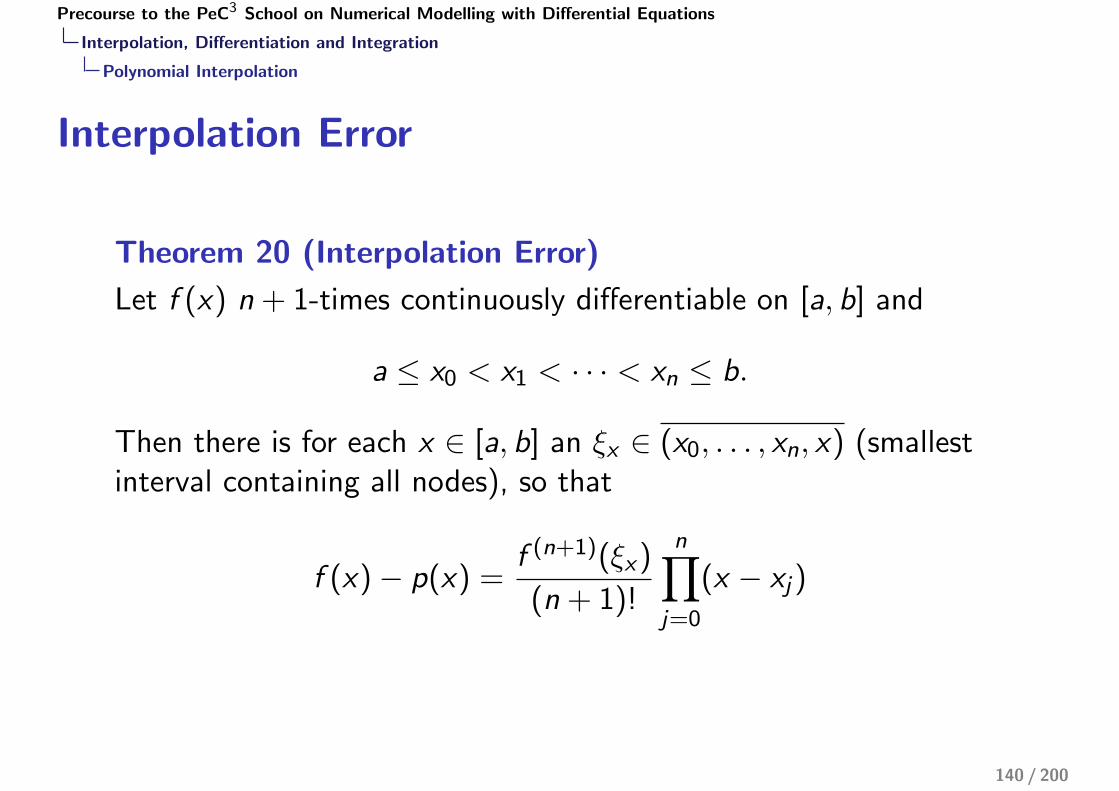
Precourse to the PeC3 School on Numerical Modelling with Differential Equations
Interpolation, Differentiation and Integration
Polynomial Interpolation
Interpolation Error
Theorem 20 (Interpolation Error)
Let f (x) n + 1-times continuously differentiable on [a, b] and
a ≤ x0 < x1 < · · · < xn ≤ b.
Then there is for each x ∈ [a, b] an ξx ∈ (x0, . . . , xn, x) (smallestinterval containing all nodes), so that
f (x)− p(x) =f (n+1)(ξx)
(n + 1)!
n�
j=0
(x − xj)
140 / 200

Precourse to the PeC3 School on Numerical Modelling with Differential Equations
Interpolation, Differentiation and Integration
Polynomial Interpolation
Remarks
For the special case of equidistant nodes, i.e.,
xk+1 − xk = h fur k = 0, . . . , n − 1,
we therefore have
|f (x)− p(x)| ≤ |f (n+1)(ξx)| · hn+1 ,
and for |f (n+1)| bounded and n → ∞ it follows |f (x)− p(x)| → 0.
Unfortunately, the higher derivatives of functions, even of simpleones, are often not bounded for n → ∞, but grow very fast instead.
141 / 200

Precourse to the PeC3 School on Numerical Modelling with Differential Equations
Interpolation, Differentiation and Integration
Polynomial Interpolation
Runge’s Counter Example
-1
-0.5
0
0.5
1
-1 -0.5 0 0.5 1
Polynomial interpolation of Runge’s function f (x) = (1 + 25x2)−1
with equidistant nodes (3, 5, 9, 17 resp. 33 node/value pairs).The minima / maxima of the last two polynomials are−14.35/1.40 resp. −5059/2.05 (!).
142 / 200

Precourse to the PeC3 School on Numerical Modelling with Differential Equations
Interpolation, Differentiation and Integration
Polynomial Interpolation
Remarks
Remark 21According to the Weierstraß Approximation Theorem, any functionin C 0([a, b]) can be approximated uniformly by polynomials.The phenomena we observe are no contradiction, since:
• The approximation need not be based on interpolation (theproof uses Bernstein polynomials).
• Using non-equidistant nodes one can already achievesignificantly improved results (if one knows how to choosethese non-equidistant nodes. . . ).
Remark 22In general “methods of higher (polynomial) order” requiresufficient differentiability.
143 / 200

Precourse to the PeC3 School on Numerical Modelling with Differential Equations
Interpolation, Differentiation and Integration
Polynomial Interpolation
Condition AnalysisWith p(x ; y) the interpolation polynomial to the values(y0, . . . , yn)
T at fixed nodes (x0, . . . , xn)T , we have
p(x ; y +Δy)− p(x ; y) =n�
i=0
(yi +Δyi )L(n)i (x)−
n�
i=0
yiL(n)i (x)
=n�
i=0
ΔyiL(n)i (x)
This implies
p(x ; y +Δy)− p(x ; y)
p(x ; y)=
n�
i=0
L(n)i (x)yip(x ; y)
· Δyiyi
For large n, L(n)i can become very large, then the interpolation task
is ill-conditioned!144 / 200

Precourse to the PeC3 School on Numerical Modelling with Differential Equations
Interpolation, Differentiation and Integration
Polynomial Interpolation
Contents I
1 Introduction to C++
2 Best Practices for Scientific Computing
3 Floating-Point Numbers
4 Condition and Stability
5 Interpolation, Differentiation and Integration
6 Solution of Linear and Nonlinear Equations
145 / 200
Precourse to the PeC3 School on Numerical Modelling with Differential Equations
Interpolation, Differentiation and Integration
Numerical Differentiation
Numerical Differentiation
Problem:Compute the derivative (of some order n) of a function that isgiven as a table or implemented as a function (in the computerscience sense of the word).
Idea:Assemble interpolation polynomial for certain nodes, differentiate itand evaluate result to obtain (approximation of) derivative.
We assume order of derivative = degree of polynomial.
146 / 200

Precourse to the PeC3 School on Numerical Modelling with Differential Equations
Interpolation, Differentiation and Integration
Numerical Differentiation
Numerical DifferentiationThe Lagrange polynomials are
L(n)i (x) =
�
j �=i
x − xjxi − xj
=�
j �=i
(xi − xj)−1
� �� �=:λi∈R
·xn + αn−1xn−1 + · · ·+ α0,
therefore taking the n-th derivative produces
dn
dxnL(n)i (x) = n! · λi
which gives us the n-th derivative of an interpolation polynomial ofdegree n:
dn
dxn
�n�
i=0
yiL(n)i (x)
�= n! ·
n�
i=0
yiλi (independent of x)
147 / 200
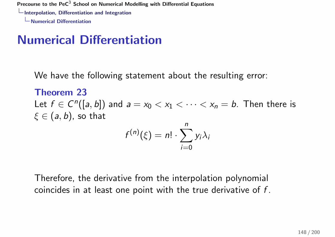
Precourse to the PeC3 School on Numerical Modelling with Differential Equations
Interpolation, Differentiation and Integration
Numerical Differentiation
Numerical Differentiation
We have the following statement about the resulting error:
Theorem 23Let f ∈ C n([a, b]) and a = x0 < x1 < · · · < xn = b. Then there isξ ∈ (a, b), so that
f (n)(ξ) = n! ·n�
i=0
yiλi
Therefore, the derivative from the interpolation polynomialcoincides in at least one point with the true derivative of f .
148 / 200

Precourse to the PeC3 School on Numerical Modelling with Differential Equations
Interpolation, Differentiation and Integration
Numerical Differentiation
Numerical DifferentiationFor equidistant nodes, xi = x0 + ih, 0 ≤ i ≤ n, there is an explicitformula based on the node values yi :
f (n)(x) ≈ h−nn�
i=0
(−1)n−i
�n
i
�yi , e.g., f (1)(x) ≈ y1 − y0
h,
f (2)(x) ≈ y2 − 2y1 + y0h2
, f (3)(x) ≈ y3 − 3y2 + 3y1 − y0h3
Based on Taylor expansion one can show
f �(x) =f (x + h)− f (x − h)
2h+O(h2) for f ∈ C 3,
f ��(x) =f (x + h)− 2f (x) + f (x − h)
h2+O(h2) for f ∈ C 4
149 / 200
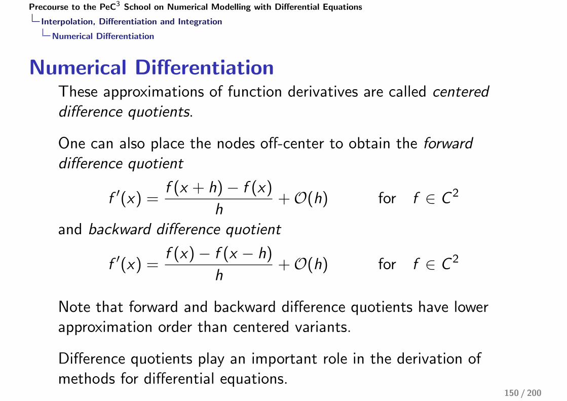
Precourse to the PeC3 School on Numerical Modelling with Differential Equations
Interpolation, Differentiation and Integration
Numerical Differentiation
Numerical DifferentiationThese approximations of function derivatives are called centereddifference quotients.
One can also place the nodes off-center to obtain the forwarddifference quotient
f �(x) =f (x + h)− f (x)
h+O(h) for f ∈ C 2
and backward difference quotient
f �(x) =f (x)− f (x − h)
h+O(h) for f ∈ C 2
Note that forward and backward difference quotients have lowerapproximation order than centered variants.
Difference quotients play an important role in the derivation ofmethods for differential equations.
150 / 200

Precourse to the PeC3 School on Numerical Modelling with Differential Equations
Interpolation, Differentiation and Integration
Extrapolation Techniques
Extrapolation to the Limit I
Let some quantity a(h) be computable for h > 0, but not for h = 0.We are interested in computing
a(0) = limh→0
a(h)
with good accuracy.
Example 24
Possible applications:
1 L’Hospital’s rule:
a(0) = limh→0
cos(x)− 1
sin(x)(= 0)
151 / 200

Precourse to the PeC3 School on Numerical Modelling with Differential Equations
Interpolation, Differentiation and Integration
Extrapolation Techniques
Extrapolation to the Limit II
Example 24
2 Numerical Differentiation:
f �(x) = limh→0
f (x + h)− f (x)
h
(small h cause cancellation)
3 Numerical Integration:
� b
af (x) = lim
N→∞
n�
i=1
N−1f
�a+ (i − 1
2)b − a
N
�
(set h := N−1)
152 / 200
Precourse to the PeC3 School on Numerical Modelling with Differential Equations
Interpolation, Differentiation and Integration
Extrapolation Techniques
Extrapolation to the Limit III
Example 24
4 Numerical solution of initial value problem
y �(t) = f (t, y(t)) on [0,T ]; y(0) = y0
Set
h = N−1; yn = yn−1 + h · f (t, yn − 1); y(T ) ≈ yN
Here h → 0 is equivalent to N → ∞ and therefore increasingcomputational cost.
153 / 200

Precourse to the PeC3 School on Numerical Modelling with Differential Equations
Interpolation, Differentiation and Integration
Extrapolation Techniques
Central Idea of Extrapolation
Idea of extrapolation:
For h0 > h1 > · · · > hn > 0 construct interpolation polynomial
p(hi ) = a(hi ) i = 0, . . . , n
and computea(0) ≈ p(0)
(Extrapolation instead of interpolation, since 0 �∈ [hn, . . . , h0])
154 / 200

Precourse to the PeC3 School on Numerical Modelling with Differential Equations
Interpolation, Differentiation and Integration
Extrapolation Techniques
Example I
Example 25
For a(h) = (cos(h)− 1) · (sin(h))−1 we have
h0 = 1/8: a(h0) = −6.258151 · 10−2
h1 = 1/16: a(h1) = −3.126018 · 10−2
h2 = 1/32: a(h2) = −1.562627 · 10−2
(i.e., a(h) is directly proptional to h), and with extrapolation usingp2 of degree 2:
a(0) ≈ p2(0) = −1.02 · 10−5
which is significantly better than the initial approximations or apossible direct evaluation for h � 1 (cancellation)!
155 / 200

Precourse to the PeC3 School on Numerical Modelling with Differential Equations
Interpolation, Differentiation and Integration
Extrapolation Techniques
Example II
Example 25
Why does this work so well?
Let hi = h · r i with r < 1 (geometric distribution), e.g., r = 1/2,and let p the interpolation polynomial of a to the nodes hi . Thenwe have
|p(0)− a(0)| ≤ �V−T�∞|a(n+1)(ξ)| hn+1
(n + 1)!(1 + rn+1)
for the extrapolation error, with Vandermonde matrix V andξ ∈ (0, h), as long as a is sufficiently differentiable.
156 / 200

Precourse to the PeC3 School on Numerical Modelling with Differential Equations
Interpolation, Differentiation and Integration
Extrapolation Techniques
Extrapolation in the Case of Derivatives
The Taylor expansion of a at zero (Mclaurin expansion) is crucial.For the usual difference quotient for the second derivative weobtain
a(h) =f (x + h)− 2f (x) + f (x − h)
h2
= f ��(x) +h2
2 · 4! f(4)(x) + · · ·+ h2n
2 · (2n + 2)!f (2n+2)(x)
+h2n+2
2 · (2n + 4)![f (2n+4)(ξ+) + f (2n+4)(ξ−)]
= px(h2) +O(h2(n+1))
This means one gains two powers of h per evaluation (if f issufficiently smooth)!
157 / 200

Precourse to the PeC3 School on Numerical Modelling with Differential Equations
Interpolation, Differentiation and Integration
Numerical Integration (Quadrature)
Newton-Cotes FormulasThe Newton-Cotes formulas are interpolatory quadrature(integration) formulas.
Idea: Construct the interpolation polynomial p of a function f forcertain nodes and evaluate the integral of p exactly to approximatethe integral of f .
Formally: nodes and values (xi , f (xi )), i = 0, . . . , n, Lagrangerepresentation:
pn(x) =n�
i=0
f (xi )L(n)i (x), L
(n)i (x) =
�
j �=i
x − xjxi − xj
and therefore
I[a,b](f ) ≈ I(n)[a,b](f ) =
� b
apn(x) dx =
n�
i=0
f (xi )
� b
aL(n)i (x) dx
158 / 200

Precourse to the PeC3 School on Numerical Modelling with Differential Equations
Interpolation, Differentiation and Integration
Numerical Integration (Quadrature)
Order of Quadrature
Definition 26 (Order of Quadrature)
A quadrature formula I (n)(f ) has at least order m, if it is able tointegrate polynomials of degree m − 1 exactly.
For example, a second order formula integrates linear functionsexactly.
The Newton-Cotes formulas use polynomial interpolation andtherefore they have at least order n + 1 for n + 1 nodes. But thereare other formulas that can achieve even higher orders with thesame number of nodes.
159 / 200

Precourse to the PeC3 School on Numerical Modelling with Differential Equations
Interpolation, Differentiation and Integration
Numerical Integration (Quadrature)
Closed and Open Formulas
The Newton-Cotes formulas use equidistant nodes. There are twovariants:
Closed formulas:The interval bounds a and b are nodes, i.e.,
xi = a+ iH, i = 0, . . . , n, with H =b − a
n
Open formulas:The bounds a and b aren’t nodes, i.e.,
xi = a+ (i + 1)H, i = 0, . . . , n, with H =b − a
n + 2
160 / 200

Precourse to the PeC3 School on Numerical Modelling with Differential Equations
Interpolation, Differentiation and Integration
Numerical Integration (Quadrature)
ExamplesClosed formulas for n = 1, 2, 3 and H = (b − a)/n:
The trapezoidal rule:
I (1)(f ) =b − a
2· [f (a) + f (b)]
The Simpson rule resp. Kepler’s barrel rule:
I (2)(f ) =b − a
6· [f (a) + 4f
�a+ b
2
�+ f (b)]
The 3/8 rule resp. “pulcherrima”:
I (3)(f ) =b − a
8· [f (a) + 3f (a + H) + 3f (b − H) + f (b)]
161 / 200

Precourse to the PeC3 School on Numerical Modelling with Differential Equations
Interpolation, Differentiation and Integration
Numerical Integration (Quadrature)
ExamplesOpen formulas for n = 0, 1, 2 and H = (b − a)/(n + 2):
The midpoint rule:
I (0)(f ) = (b − a) · f�a+ b
2
�
The second open rule (no special name):
I (1)(f ) =b − a
2· [f (a + H) + f (b − H)]
The third open rule (also no special name):
I (2)(f ) =b − a
3· [2f (a)− f
�a+ b
2
�+ 2f (b)]
162 / 200
Precourse to the PeC3 School on Numerical Modelling with Differential Equations
Interpolation, Differentiation and Integration
Numerical Integration (Quadrature)
Remarks
Remark 27From n = 7 on for closed rules, resp. from n = 2 on for open rules,negative weights appear in the sums. This is detrimental, because:
• Strictly non-negative functions f can have I (n)(f ) < 0 (soluteconcentration, mass conservation,. . . ).
• There is increased risk of cancellation.
• Condition can become worse, while it is bounded for strictlypositive weights.
163 / 200

Precourse to the PeC3 School on Numerical Modelling with Differential Equations
Interpolation, Differentiation and Integration
Numerical Integration (Quadrature)
Estimates for Remainder Terms I
Theorem 28 (Remainder Terms)
The resulting error can be estimated as follows:
1 Trapezoidal rule: n = 1, order 2, we have
I (f )− b − a
2· [f (a) + f (b)] = −(b − a)3
12f ��(ξ), ξ ∈ [a, b]
for f ∈ C 2([a, b]). This means polynomials up to degree 1 areintegrated exactly, because for those f ��(x) = 0 holds on [a, b].
In general: the order of the odd formulas is the number ofnodes, while the order of the even formulas is one higher.
164 / 200

Precourse to the PeC3 School on Numerical Modelling with Differential Equations
Interpolation, Differentiation and Integration
Numerical Integration (Quadrature)
Estimates for Remainder Terms II
Theorem 28 (Remainder Terms)
2 Simpson rule: n = 2, order 4, for f ∈ C 4([a, b]) we have
I (f )− b − a
6· [f (a)+4f
�a+ b
2
�+ f (b)] = −(b − a)5
2880f (4)(ξ)
3 Midpoint rule: n = 0, order 2, for f ∈ C 2([a, b]) we have
I (f )− (b − a) · f�a+ b
2
�=
(b − a)3
24f ��(ξ)
so “half the error of trapezoidal rule” at just one functionevaluation!
165 / 200
Precourse to the PeC3 School on Numerical Modelling with Differential Equations
Interpolation, Differentiation and Integration
Numerical Integration (Quadrature)
Summed Quadrature Rules
Increasing the polynomial degree doesn’t make much sense, since
• negative weights appear early
• Lagrange interpolation with equidistant nodes doesn’tconverge pointwise
• f has to be sufficiently regular for the estimates to hold
Idea of summed quadrature rules:
• Subdivide interval [a, b] into N smaller intervals
[xi , xi+1], xi = a+ ih, i = 0, . . . ,N − 1, h =b − a
N
• Apply one of the above formulas on each subinterval and sumthe results.
166 / 200

Precourse to the PeC3 School on Numerical Modelling with Differential Equations
Interpolation, Differentiation and Integration
Numerical Integration (Quadrature)
ExamplesFor N subintervals of stepsize h we arrive at:
The summed trapezoidal rule:
I(1)h (f ) =
N−1�
i=0
h
2[f (xi ) + f (xi+1)] = h ·
�f (a)
2+
N−1�
i=1
f (xi ) +f (b)
2
�
The summed Simpson rule:
I(2)h (f ) =
h
3·�f (a)
2+
N−1�
i=1
f (xi ) + 2N−1�
i=1
f
�xi + xi+1
2
�+
f (b)
2
�
The summed midpoint rule:
I(0)h (f ) = h ·
N−1�
i=0
f
�xi + xi+1
2
�
167 / 200

Precourse to the PeC3 School on Numerical Modelling with Differential Equations
Solution of Linear and Nonlinear Equations
Contents I
1 Introduction to C++
2 Best Practices for Scientific Computing
3 Floating-Point Numbers
4 Condition and Stability
5 Interpolation, Differentiation and Integration
6 Solution of Linear and Nonlinear Equations
168 / 200

Precourse to the PeC3 School on Numerical Modelling with Differential Equations
Solution of Linear and Nonlinear Equations
Introduction
Vectors and Matrices IA vector v ∈ Rn is a finite sequence of real numbers:
v = [v1, v2, . . . , vn]T , vi ∈ R
A matrix A ∈ Rn×m is defined similarly, but uses two independentindices i and j , one for columns and one for rows:
A =
a11 a12 · · · a1ma21 a22 · · · a2m...
.... . .
...an1 an2 · · · anm
, aij ∈ R
Each matrix A ∈ Rn×m corresponds to a linear mappingϕA : Rm → Rn given by
ϕA(v) = A · v , v ∈ Rm
169 / 200

Precourse to the PeC3 School on Numerical Modelling with Differential Equations
Solution of Linear and Nonlinear Equations
Introduction
Vectors and Matrices IIFor a sufficiently regular scalar function f (x), x = [x1, . . . , xm], wehave the following special vectors and matrices:
∇f :=
�∂f
∂x1, . . . ,
∂f
∂xm
�T(gradient)
Hf = ∇2f :=
�∂2f
∂xi∂xj
�
ij
(Hessian)
For vector-valued functions f (x) = [f1(x), . . . , fn(x)]T , the gradient
generalizes to the Jacobian:
Jf =
�∂fi∂xj
�
ij
If f = ϕA is a linear function, then Jf = A, i.e., the constituentmatrix A and the Jacobian coincide. 170 / 200

Precourse to the PeC3 School on Numerical Modelling with Differential Equations
Solution of Linear and Nonlinear Equations
Introduction
Natural Matrix Norms
Definition 29 (Associated Matrix Norm)
Let � · � an arbitrary vector norm on Rn. Then
�A� := supx∈Rn\{0}
�Ax��x� = sup
x∈Rn,�x�=1�Ax�
is called the matrix norm associated with � · �, or natural matrixnorm. It is compatible with the matrix norm, i.e.,
�Ax� ≤ �A� · �x� A ∈ Rn×n, x ∈ Rn,
and submultiplicative, i.e.,
�AB� ≤ �A� · �B� A,B ∈ Rn×n
(compare with triangle inequality / subadditivity).171 / 200

Precourse to the PeC3 School on Numerical Modelling with Differential Equations
Solution of Linear and Nonlinear Equations
Introduction
Linear and Nonlinear Systems of Equations
Many important problems, e.g., the solution of ordinary and partialdifferential equations, can be framed as solving a given linearsystem of equations:
A · x = b resp. A · x − b = 0
or nonlinear system of equations:
F (x) = 0
where F is a possibly vector-valued function, A is a matrix, and xand b are vectors of the right dimensions.
172 / 200
Precourse to the PeC3 School on Numerical Modelling with Differential Equations
Solution of Linear and Nonlinear Equations
Introduction
Perturbation Theorem
Theorem 30 (Perturbation Theorem)
Let A ∈ Rn×n regular and �ΔA� ≤ �A−1�−1. Then �A = A+ΔA is
also regular, and for the relative error of the perturbed system
(A+ΔA) · (x +Δx) = b +Δb
the equation
�Δx��x� ≤ cond(A)
1− cond(A) · �ΔA��A�
·��Δb�
�b� +�ΔA��A�
�
holds, where cond(A) := �A� · �A−1� is the condition number ofthe matrix A. For the special case ΔA = 0 we have
�Δx��x� ≤ cond(A) · �Δb�
�b� .173 / 200

Precourse to the PeC3 School on Numerical Modelling with Differential Equations
Solution of Linear and Nonlinear Equations
Direct Solvers for Linear Systems
Triangular Systems
Let A ∈ Kn×n an upper triangular matrix:
a11 · x1 + a12 · x2 + · · ·+ a1n · xn = b1
a22 · x2 + · · ·+ a2n · xn = b2
. . ....
...
ann · xn = bn
This system permits a unique solution iff aii �= 0, i = 1, . . . , n.
Because of the simple structure this can be solved using “backwardsubstitution”.
174 / 200

Precourse to the PeC3 School on Numerical Modelling with Differential Equations
Solution of Linear and Nonlinear Equations
Direct Solvers for Linear Systems
Triangular SystemsSolution using backward substitution:
xn = bn/ann
xn−1 =�bn−1 − a(n−1)n · xn
�/a(n−1)(n−1)
...
xi =
�bi −
n�
k=i+1
aik · xk�/aii
Required number of operations:
NΔ(n) =n−1�
i=0
(2i + 1) = n2
(Of course there is an analogous “forward substitution” for uppertriangular matrices.) 175 / 200

Precourse to the PeC3 School on Numerical Modelling with Differential Equations
Solution of Linear and Nonlinear Equations
Direct Solvers for Linear Systems
Direct Methods for Linear Systems
Let A ∈ Kn×n regular, but with arbitrary structure.
Goal: Transform A into (upper) triangular form, then use backwardsubstitution.
This can be done using:
• exchange of two equations / rows
• addition of a multiple of one equation to another
This is a standard technique known as Gauss elimination.
176 / 200
Precourse to the PeC3 School on Numerical Modelling with Differential Equations
Solution of Linear and Nonlinear Equations
Direct Solvers for Linear Systems
Gauss Elimination
Perform the following steps until an upper triangular matrix isobtained, starting with k = 1:
1 For i > k , define lik = aik · a−1kk .
2 For i > k , setaij ←− aij − likakj
(subtract a multiple of the k-th row to eliminate the first kentries of the i-th row).
3 Increase k by one: k ←− k + 1.
4 Repeat.
After (at most) n − 1 loop iterations the matrix has become upperright triangular.
177 / 200

Precourse to the PeC3 School on Numerical Modelling with Differential Equations
Solution of Linear and Nonlinear Equations
Direct Solvers for Linear Systems
Cost of Gauss Elimination
Lemma 31The cost of transforming A into an upper right triangular matrixby Gauss elimination is
NGauß(n) =2
3n3 +O(n2)
Since the cost for backward substitution is negligible(NΔ(n) = n2), this is also the cost for solving a linear equationsystem using Gauss elimination.
178 / 200

Precourse to the PeC3 School on Numerical Modelling with Differential Equations
Solution of Linear and Nonlinear Equations
Direct Solvers for Linear Systems
A Note on Stability
The classic Gauss elimination is unstable for general matrices(because we divide by diagonal elements of the original matrix,which can become arbitrarily small).
The algorithm can be made significantly more stable through aprocess called row pivotisation. In each iteration, we search for thelargest subdiagonal element in the k-th column and swap its rowwith the k-th row, remembering resulting row permutations.
Total pivotisation instead searches for the largest element in thelower right corner of the matrix, and employs both row and columnpermutations. This is more expensive, but leads to furtherimprovements in terms of stability.
179 / 200

Precourse to the PeC3 School on Numerical Modelling with Differential Equations
Solution of Linear and Nonlinear Equations
Direct Solvers for Linear Systems
LU Decomposition I
Storing the factors lik of the elimination steps is a good idea:
Theorem 32 (LU Decomposition)
Let A ∈ Rn×n regular, then there exists a decomposition PA = LU,where
L =
1 0 · · · 0
l11 1. . .
......
. . .. . . 0
ln1 · · · ln(n−1) 1
, U =
u11 u12 · · · u1n
0 u22. . . u2n
.... . .
. . . u(n−1)n
0 · · · 0 unn
,
and P is a permutation matrix. For P = I this decomposition isunique.
180 / 200

Precourse to the PeC3 School on Numerical Modelling with Differential Equations
Solution of Linear and Nonlinear Equations
Direct Solvers for Linear Systems
LU Decomposition II
Solving a linear system via LU decomposition:
1 For given A, compute LU decomposition and matrix P
2 For given b, calculate b� = Pb
3 Solve triangular system Ly = b� (forward substitution)
4 Solve triangular system Rx = y (backward substitution)
LU decomposition is equivalent to Gauss elimination, and thereforehas the same cost NLU(n) =
23n
3 +O(n).
Important difference:The LU decomposition can be reused for new righthand sidesA�x = �b, while Gauss elimination has to start over from thebeginning!
181 / 200

Precourse to the PeC3 School on Numerical Modelling with Differential Equations
Solution of Linear and Nonlinear Equations
Direct Solvers for Linear Systems
Symmetric Positive Definite Matrices
Theorem 33For a symmetric positive definite (s.p.d.) matrix A ∈ Rn×n the LUdecomposition is always stable, even without pivotisation. Theequation
a(k)ii ≥ λmin(A), k ≤ i ≤ n
holds for the diagonal elements, where λmin(A) is the smallesteigenvalue of A.
The symmetric structure of the matrix can be used to reduce thecost of LU decomposition.
182 / 200

Precourse to the PeC3 School on Numerical Modelling with Differential Equations
Solution of Linear and Nonlinear Equations
Direct Solvers for Linear Systems
Cholesky DecompositionWith D = diag(R) we have
A = LD(D−1R) = LDR with R := D−1U,
and because of symmetry R = LT , therefore A = LDLT . Since alldiagonal elements of D are positive, the matrix D1/2 with
(D1/2)ii = d1/2ii , (D1/2)ij = 0 for i �= j
is well-defined, and
A = LD1/2 · D1/2LT = �L�LT with �L := LD1/2
holds.
This special form of the decomposition is called Choleskydecomposition, it has half the cost of the general version.
183 / 200

Precourse to the PeC3 School on Numerical Modelling with Differential Equations
Solution of Linear and Nonlinear Equations
Iterative Methods for Linear Systems
Iterative Methods for Linear Systems IWe consider a second approach for the solution of
Ax = b, A ∈ Rn×n regular, b ∈ Rn.
Definition 34 (Sparse Matrices)
A sequence of matrices {A(n) | n ∈ N} is called sparse, iff
|{a(n)ij | a(n)ij �= 0}| =: nnz(A(n)) = O(n)
(nnz = “number of non-zeros”).
Because of “fill in” Gauss elimination is often unsuited for sparsematrices, and: for large systems the cost in O(n3) makes thesolution intractable.
184 / 200
Precourse to the PeC3 School on Numerical Modelling with Differential Equations
Solution of Linear and Nonlinear Equations
Iterative Methods for Linear Systems
Iterative Methods for Linear Systems IIWe have
Solving Ax = b ⇐⇒ “root search” for f (x) := b − Ax = 0.
With given matrix C , define the iteration
x (t+1) = g(x (t)) = x (t) + C−1f (x (t))
= x (t) + C−1(b − Ax (t))
= (I − C−1A)� �� �=:B
x (t) + C−1b
with “iteration matrix” B . The choice C = A would be optimal intheory, but that requires solving the problem itself.
=⇒ look for easily invertible C “similar” to A185 / 200

Precourse to the PeC3 School on Numerical Modelling with Differential Equations
Solution of Linear and Nonlinear Equations
Iterative Methods for Linear Systems
Iterative Methods for Linear Systems III
For the solution x := A−1b,
g(x) := (I − C−1A)x + C−1b = x − (C−1A) · (A−1b) + C−1b = x
holds, therefore x is a fixpoint of g .
The Lipschitz constant of the function g fulfills
�g(x)− g(y)� = �B(x − y)� ≤ �B� · �x − y�,
i.e., if �B� < 1 (for suitable matrix norm � · �), then g is acontraction on Rn, and repeated application of g defines asequence that converges to the solution (consequence of Banach’sfixpoint theorem).
186 / 200

Precourse to the PeC3 School on Numerical Modelling with Differential Equations
Solution of Linear and Nonlinear Equations
Iterative Methods for Linear Systems
Examples for Iterative MethodsDecompose A = L+D +U with L strict lower triangular matrix, Ddiagonal matrix and U strict upper triangular matrix.
Jacobi method:Set C = D, i.e.,
x (t+1) = x (t) + D−1(b − Ax (t))
Gauß–Seidel method:Set C = L+ D, i.e., (forward substitution)
x (t+1) = x (t) + (L+ D)−1(b − Ax (t))
Such iterative methods typically converge only for special classes ofmatrices (since we need �B� < 1).
187 / 200

Precourse to the PeC3 School on Numerical Modelling with Differential Equations
Solution of Linear and Nonlinear Equations
Iterative Methods for Linear Systems
Convergence of Jacobi Method
A matrix is called strictly diagonally dominant, iff
�
j �=i
|aij | < |aii | ∀ i = 1, . . . , n.
Theorem 35The Jacobi method converges for strictly diagonally dominantmatrices.
There are many similar statements for symmetric positive definitematrices, weakly diagonally dominant matrices, so-calledM-matrices, . . .
188 / 200

Precourse to the PeC3 School on Numerical Modelling with Differential Equations
Solution of Linear and Nonlinear Equations
Iterative Methods for Linear Systems
Costs
Let α(n) be the cost for one iteration, typically with α(n) = O(n).Since
�x (t) − x� ≤ �B�t�x (0) − x�,
a total of t ≥ log(�)log(�B�) iterations are necessary for a reduction of
the error by a factor � � 1, leading to a total cost of
Tfix(n) =log(�)
log(�B�)α(n).
Problem: high costs if �B� is close to one, �B� is problemdependent and often grows with n.
189 / 200

Precourse to the PeC3 School on Numerical Modelling with Differential Equations
Solution of Linear and Nonlinear Equations
Iterative Methods for Linear Systems
Conjugate Gradients
For symmetric positive definite matrices A one can instead use themethod of Conjugate Gradients. It uses an initial guess x0, theinitial residuum r0 := b − Ax0, and d0 := r0 to iteratively compute
αt =rTt rt
dTt Adt
xt+1 = xt + αtdt
rt+1 = rt − αtAdt
βt =rTt+1rt+1
rTt rt
dt+1 = rt+1 + βtdt
• The CG method convergesin at most n steps in exactarithmetic.
• For n � 1 it can be used asan iterative method, andoften displays goodconvergence properties afterthe first few steps.
190 / 200

Precourse to the PeC3 School on Numerical Modelling with Differential Equations
Solution of Linear and Nonlinear Equations
Newton’s Method for Nonlinear Systems
Newton’s MethodLet f a differentiable function in onevariable. For given xt we have the“tangent”
Tt(x) = f �(xt)(x − xt) + f (xt)
with root
Tt(x) = 0 ⇐⇒ x = xt −f (xt)
f �(xt). x t+1x t
Using this root as an estimate for the root of f leads to theiteration
xt+1 = xt −f (xt)
f �(xt).
Obviously we need |f �(xt)| > 0, i.e., we assume that the root of fis a simple root.
191 / 200

Precourse to the PeC3 School on Numerical Modelling with Differential Equations
Solution of Linear and Nonlinear Equations
Newton’s Method for Nonlinear Systems
Newton’s Method in Multiple DimensionsNewton’s method can be extended to systems f : Rn → Rn:
Assume that the Taylor expansion of f exists:
fi (x) = fi (xt+Δx) = fi (xt)+n�
j=1
∂fi∂xj
(xt)Δxi+Ri (xt ,Δx) i = 1, . . . , n
or in vector notation
f (xt +Δx) = f (xt) + Jf (xt)Δx + R(xt ,Δx)
with “Jacobian” matrix
[Jf (xt)]ij =∂fi∂xj
(xt)
192 / 200

Precourse to the PeC3 School on Numerical Modelling with Differential Equations
Solution of Linear and Nonlinear Equations
Newton’s Method for Nonlinear Systems
Newton’s Method in Multiple Dimensions
Ignoring the remainder term is equivalent to “linearization of f ”.Find approximate root of f :
f (x) ≈ f (xt) + Jf (xt)Δx = 0 ⇐⇒ Δx = −J−1f (xt)f (xt)
This leads to the iteration
xt+1 = xt − J−1f (xt)f (xt)
Every single step requires the solution of a linear system based onthe local Jacobian!
193 / 200
Precourse to the PeC3 School on Numerical Modelling with Differential Equations
Solution of Linear and Nonlinear Equations
Newton’s Method for Nonlinear Systems
Convergence of Newton’s Method I
Theorem 36 (Newton’s Method)
Let f ∈ C 2([a, b]) have a root z in (a, b) (interior!), and let
m := mina≤x≤b
|f �(x)| > 0, M := maxa≤x≤b
|f ��(x)|.
Let ρ > 0 chosen thus, that
q :=M
2mρ < 1, Kρ(z) := {x ∈ R | |x − z | ≤ ρ} ⊂ [a, b]
Then for every initial value x0 ∈ Kρ(z) the Newton iterationsxt ∈ Kρ(z) are defined and converge to the root z .
194 / 200

Precourse to the PeC3 School on Numerical Modelling with Differential Equations
Solution of Linear and Nonlinear Equations
Newton’s Method for Nonlinear Systems
Convergence of Newton’s Method II
Theorem 36 (Newton’s Method)
Additionally, the a priori error erstimate
|xt − z | ≤ 2m
Mq(2
t), t ∈ N
and the a posteriori error estimate
|xt − z | ≤ m−1|f (xt)| ≤M
2m|xt − xt−1|2, t ∈ N.
hold (a priori: only uses prerequisites, a posteriori: also usesiterations that were computed up to that point)
195 / 200

Precourse to the PeC3 School on Numerical Modelling with Differential Equations
Solution of Linear and Nonlinear Equations
Newton’s Method for Nonlinear Systems
Example: Roots of Real Numbers
Example 37 (Computing Roots with Newton’s Method)
Let a > 0 and n ≥ 1. Solve xn = a, i.e.,
f (x) = xn − a = 0, f �(x) = n · xn−1.
This leads to iteration
xt+1 = n−1 · [(n − 1) · xt + a · x1−nt ].
According to Thm. 36 this converges, if x0 is close enough to a1/n.However, in this special case it converges globally, i.e., for allx0 > 0 (but not necessarily quadratically in the beginning).
196 / 200

Precourse to the PeC3 School on Numerical Modelling with Differential Equations
Solution of Linear and Nonlinear Equations
Newton’s Method for Nonlinear Systems
Remarks I
Remark 38
• Newton’s method converges only locally, i.e., when|x0 − z | ≤ ρ (“basin of attraction”). Here ρ is normally notknown and potentially very small.
• Newton’s method exhibits quadratic convegence,
|xt − z | ≤ c · |xt−1 − z |2,
in contrast to alternatives like, e.g., bisection, whichconverges only linearly.
197 / 200

Precourse to the PeC3 School on Numerical Modelling with Differential Equations
Solution of Linear and Nonlinear Equations
Newton’s Method for Nonlinear Systems
Remarks II
Remark 38
• Damped Newton’s method:Convergence outside of the basin of attraction can beimproved by setting
xt+1 = xt − λtf (xt)
f �(xt)
with the choice of some sequence λt ∈ (0, 1] as “dampeningstrategy”.
198 / 200

Precourse to the PeC3 School on Numerical Modelling with Differential Equations
Solution of Linear and Nonlinear Equations
Newton’s Method for Nonlinear Systems
Remarks III
Remark 38
• Multiple roots:If z is a p-fold root, with p > 1, Newton’s method will stillconverge, but only linearly. One can show that the modifiediteration
xt+1 = xt − p · f (xt)f �(xt)
reestablishes quadratic convergence if p is known a priori.
199 / 200

Precourse to the PeC3 School on Numerical Modelling with Differential Equations
Solution of Linear and Nonlinear Equations
Newton’s Method for Nonlinear Systems
Summary
In the last few days, we have discussed the fundamentals of thefollowing topics:
1 Numerical programming in C++
2 Numbers and calculations with finite precision
3 Condition analysis of numerical problems and tasks
4 Error propagation and stability of numerical algorithms
5 Numerical differentiation and integration
6 Numerical solution of linear and nonlinear equation systems
The introduced concepts will form the basis of the lectures andexercises next week.
200 / 200
Recommended