Predicting Bad Patents: Employing Machine Learning toPredict Post-Grant Review Outcomes for US Patents
David Winer
Electrical Engineering and Computer SciencesUniversity of California at Berkeley
Technical Report No. UCB/EECS-2017-60http://www2.eecs.berkeley.edu/Pubs/TechRpts/2017/EECS-2017-60.html
May 11, 2017

Copyright © 2017, by the author(s).All rights reserved.
Permission to make digital or hard copies of all or part of this work forpersonal or classroom use is granted without fee provided that copies arenot made or distributed for profit or commercial advantage and that copiesbear this notice and the full citation on the first page. To copy otherwise, torepublish, to post on servers or to redistribute to lists, requires priorspecific permission.

PREDICTING BAD PATENTS 1
Predicting Bad Patents: Employing Machine Learning to Predict Post-Grant Review
Outcomes for US Patents
2017 Master of Engineering Capstone Report
University of California, Berkeley
14th April 2017
Written by David Winer, Department of Electrical Engineering and Computer Sciences
In collaboration with:
William Ho, Department of Electrical Engineering and Computer Sciencs
Joong Hwa Lee, Department of Electrical Engineering and Computer Sciences
Dany Srage, Department of Industrial Engineering and Operations Research
Tzuo Shuin Yew, Department of Electrical Engineering and Computer Sciences
Faculty Advisor: Lee Fleming, Department of Industrial Engineering and Operations Research
Faculty Committee Member: Vladamir Stojanovic, Department of Electrical Engineering and
Computer Sciences

PREDICTING BAD PATENTS 2
Table of Contents
I. Executive Summary ..................................................................................................................... 3
II. Individual Technical Contributions ............................................................................................ 4
Project overview ......................................................................................................................... 4
Wrangling PTAB case data ......................................................................................................... 6
Engineering appropriate features for PTAB case data ................................................................ 8
Model choice: Support vector classification and random forest ............................................... 11
Support vector classification ................................................................................................. 11
Random forest classification ................................................................................................. 12
Results and discussion .............................................................................................................. 14
Classifier results .................................................................................................................... 14
Limitations of analysis and discussion ................................................................................. 18
Conclusion and discussion of future work ................................................................................ 20
III. Engineering Leadership .......................................................................................................... 21
Introduction and project overview ............................................................................................ 21
Designing a tailored marketing strategy ................................................................................... 21
Competition in the patent analytics space ................................................................................. 23
Review of machine learning technology trends ........................................................................ 24
Ethical challenges associated with patent prediction ................................................................ 25
Engineering leadership conclusions .......................................................................................... 26
References ..................................................................................................................................... 27
Appendix ....................................................................................................................................... 30
Section A: How will the invalidation prediction algorithm help the US Patent and Trademark
Office?....................................................................................................................................... 30
Section B: Additional figures.................................................................................................... 30
Section C: Denial prediction code ............................................................................................ 33

PREDICTING BAD PATENTS 3
I. Executive Summary
As the number of patents filed with the US Patent Office has ballooned over the last two
decades, the need for more powerful patent analytics tools has grown stronger. In 2012, the US
Federal Government’s America Invents Act (AIA) put into place a new post-grant review process
by which any member of the public could challenge an existing patent through the Patent Trials
and Appeal Board (PTAB). Our capstone team has developed a tool to predict outcomes for this
post-grant review process. We developed algorithms to predict two major outcomes: whether a
case brought by a member of the public will be accepted by the Patent Trials and Appeal Board
and, once that case is accepted, whether the relevant patent will be invalidated by the Board.
In this report, I focus on the former algorithm—acceptance vs. denial prediction. To predict
case acceptance/denial we use natural language processing (NLP) techniques to convert each
litigated patent document into thousands of numeric features. Upon combining these text-based
features with patent metadata, we used two primary machine learning algorithms to attempt to
classify these documents based on their case acceptance/denial outcome: support vector
classification and random forests. In this report, I focus both on the efforts we went through to
wrangle the data as well as the hyperparameters we tuned across these two algorithms. We found
that we were able to achieve performant algorithms that exhibited classification accuracy slightly
better than the base rate data skew, although further room for improvement exists. As the post-
grant review process matures, there will be further opportunity to gather more case data, refine the
tools we have built over the past year, and increase the confidence associated with post-grant
review analytics.

PREDICTING BAD PATENTS 4
II. Individual Technical Contributions
Project overview
Over the last two decades, the pace of innovation in the United States, and correspondingly,
the number of patents filed with the US Patent and Trademark Office, has grown dramatically. In
2014, 300,000 patents were filed with the US Patent and Trademark office, and this number
continues to grow every year (U.S. Patent Statistics Chart, 2016). This rise in the number of patents
has also led to a corresponding increase in the quantity of human and financial resources spent on
patent filing, post-grant review, and litigation. The focus of our capstone project has been on
building a machine learning tool for patent applicants and examiners to predict the outcomes of
post-grant review for their patents (e.g., the probability that a case would be litigated before the
Patent Trials and Appeal Board (PTAB) if the patent were challenged, and whether that case would
be successful). By providing this information before patents are approved, we hope to limit the
cost that bad patents impose on the legal system and the economy—estimated to be up to $26
billion every year (Beard, Ford, Koutsky, & Spiwak, 2010, p. 268).
Our project had three main phases: data collection, machine learning model design, and
application creation (Figure 1). In the data collection phase, we gathered the data needed to train
our machine learning algorithms—prediction of trial outcomes from the US PTAB (which
comprise our independent variables) and the text associated with each contested patent (our
dependent variable, along with additional metadata associated with each case). My teammates
William Ho and Joong Hwa Lee led these data wrangling efforts and discuss in their reports,
respectively, our team’s use of existing APIs for gathering data as well as the less-structured PDF
data that we parsed in order to gather metadata features. In the modeling phase, we built upon
existing machine learning and natural language processing technologies to construct a machine

PREDICTING BAD PATENTS 5
learning algorithm that can use text data to predict the likelihood of two outcomes: case
acceptance/denial and invalidation. Case acceptance/denial refers to the initial outcome for a case
brought before the PTAB—whether the Board agrees to hear the case or not (Marco 2016). Cases
that are denied cannot be subsequently be brought before the PTAB for invalidation hearings. Only
once a case is accepted can it then be ruled on as valid or invalid. My teammate Dany Srage led
the design of the invalidation algorithm and discusses that algorithm in his report, while I will
focus on the acceptance/denial algorithm. Finally, after creating and evaluating machine learning
algorithms to predict both of these outcomes, we designed and deployed a web GUI application
that predicts the likelihood of invalidation for a given patent uploaded by the user. My teammate
TS Yew led the design of the web application we used to make our two algorithms publicly
available and discusses that work in greater detail in his report.
My primary contribution to the project involved predicting whether a case will be accepted
or denied by the Patent Trial and Appeals Board (hereafter referred to as the “denials algorithm”).
In this report, I will discuss the different steps taken to develop this algorithm, in particular:
wrangling the PTAB case and patent text data necessary for this algorithm, selecting and tuning
models appropriate for the task, and evaluating the outcomes of each model.
Figure 1: Predicting Bad Patents project breakdown—focus of this report highlighted in blue
Algorithm design and
evaluation
Data collection Invalidation algorithm
Case
acceptance/denial
algorithm
Algorithm
deployment
1 2 3
PREDICTING BAD PATENTS 6
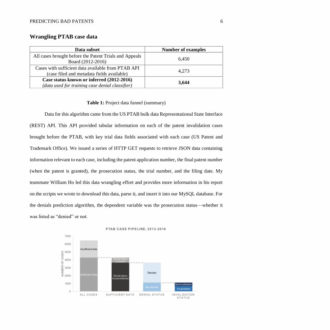
Wrangling PTAB case data
Data subset Number of examples
All cases brought before the Patent Trials and Appeals
Board (2012-2016) 6,450
Cases with sufficient data available from PTAB API
(case filed and metadata fields available) 4,273
Case status known or inferred (2012-2016)
(data used for training case denial classifier) 3,644
Table 1: Project data funnel (summary)
Data for this algorithm came from the US PTAB bulk data Representational State Interface
(REST) API. This API provided tabular information on each of the patent invalidation cases
brought before the PTAB, with key trial data fields associated with each case (US Patent and
Trademark Office). We issued a series of HTTP GET requests to retrieve JSON data containing
information relevant to each case, including the patent application number, the final patent number
(when the patent is granted), the prosecution status, the trial number, and the filing date. My
teammate William Ho led this data wrangling effort and provides more information in his report
on the scripts we wrote to download this data, parse it, and insert it into our MySQL database. For
the denials prediction algorithm, the dependent variable was the prosecution status—whether it
was listed as “denied” or not.

PREDICTING BAD PATENTS 7
Figure 2: Visual representation of data pipeline
To acquire the text of the patents, we used an existing UC Berkeley Fung Institute MySQL
database containing the text of all US patents from 1976-2015. For each of our patent cases, we
submitted a SQL query to the Fung database to retrieve all relevant claims associated with that
patent. After retrieving these claims, we merged them together using simple string concatenation
in Python.
Of these cases, we found that not all of them actually had a relevant denial status—56% of
them had a null value in this field (Patent Trial and Appeal Board). The breakdown of cases from
the raw data extracted from the API is shown in Table 2.
Value Proportion
Total PTAB cases 4273 100%
Denied status provided 2490 58%
No status 1783 42%
Table 2: PTAB cases by denial status (raw data)
It was surprising that over 40% of the patent cases had missing case statuses. We expected
this tag to be unpopulated for currently in-progress cases, but this set comprised a small minority
of the data. Specifically, we found that in almost no cases did the PTAB allow more than 200 days
to elapse from filing to decision due to regulations set forth by the US Patent Office (Figure 3);
however, only 15% of the cases in the dataset had been filed fewer than 200 days before the data
was downloaded. As a result, we concluded that a number of the cases had missing statuses due to
reporting errors. To correct for this missing data, we employed the heuristic that any cases that
were filed outside of the prior 200 days must have been either accepted or denied. For those in this
set that had no invalidation decision reported or relevant invalidation documents, we assumed that
those cases had been denied—a conclusion also supported by the PTAB’s published figures on

PREDICTING BAD PATENTS 8
how many cases it has accepted and ruled on (Patent Trial and Appeal Board Statistics). This
approach increased the number of patents in our training dataset from 2,490 to 3,644, as shown in
Table 3, and visually represented in Figure 2.
Value Proportion
Total PTAB cases 4273 100%
Denied status provided
or inferred 3644 85%
No status 629 15%
Table 3: PTAB cases by denial status (wrangled data)
Figure 3: Time from case filing to decision (raw data)
Engineering appropriate features for PTAB case data
Our approach to variable extraction for the denials algorithm was relatively
straightforward. For each patent, we used word frequencies to create thousands of numeric
features. We replicated this method for bigrams (ordered pairs of words), trigrams (ordered triplets
of words), and tetragrams (ordered quadruplets). As shown in Figure 4, each linear increase in the

PREDICTING BAD PATENTS 9
number of words included in the feature led to an exponential increase in the number of features—
and therefore the complexity of the model.
This naïve approach is known as the “bag of words” or “bag of phrases” method (Cambria
and White, 2014, p.50). We found, for a subset of our data, however, that this approach gave far
too much weight to common but relatively non-informative words. Accordingly, we implemented
an approach called term frequency-inverse document frequency (TF-IDF). This method takes our
simple bag-of-words frequency variables and normalizes them based on the frequency with which
each word is used across all patents (Berger and Lafferty, 2016, p.5). As a result, each word
frequency score in a given patent represents how rare that word is within the patent relative to the
set of all patents. This approach ensures that the variables that we are feeding into our statistical
model truly measure the differences across the full corpus of US patents and do not give undue
weight to common but non-predictive words. Additionally, prior to applying the TFIDF
transformation to our data, we stripped out stop-words like “the” and “and,” which we anticipated
would add more noise to our model than predictive power.
Additionally, we had to handle the fact that words with the same root (e.g., “hop,”
“hopping,” “hopped”) would count as separate features in the algorithm even though they likely
reflect the same concept across different patents in the corpus. To resolve this issue, we used the
Natural Language Toolkit (NLTK) Snowball Stemmer to use stem words as features (NLTK
2016). This approach essentially reduced each variation on the root of a word down to its word
stem. In the example provided above, the Stemmer would map the words “hop,” “hopping,” and
“hopped” to the same word feature—“hop.”
Finally, we used a latent semantic analysis approach for dimensionality reduction. By
computing the singular value decomposition of our tetragram model and choosing the top N

PREDICTING BAD PATENTS 10
features (where N = 1K, 5K, 10K, and 20K) from this decomposition, we were able to reduce the
level of complexity introduced from the n-gram approach described above. Mathematically, this
approach works by computing a change of basis from the original set of features and selecting the
top N most informative dimensions—i.e., the dimensions that harbor the greatest variation among
the different patents (Landauer, Foltz, & Laham, 1998). Results from these dimensionality
reduction efforts are shown in Figure 5.
Finally, after performing text featurization, we included the patent art unit and examiner as
metadata fields. The wrangling conducted to gather these data fields is further discussed by my
teammates William Ho and Dany Srage in their reports.
After these featurization techniques, we split the data by setting aside 80% of it as our
training dataset and leaving aside the remaining 20% for evaluation (our test set). This approach
allowed us to ensure that our model has sufficient generalizability and is not over-fit on the data it
was trained on.
Figure 4: Model complexity increases exponentially with each word added to n-grams

PREDICTING BAD PATENTS 11
Model choice: Support vector classification and random forest
For the denials algorithm, we tested out two very different machine learning models: support
vector classification and random forest classification. We chose these models for their simplicity
and the fact that the underlying statistical classification methods are different enough between
them that they would provide us some variety in our approach to classification. I will discuss each
of them in turn.
Support vector classification
This approach maps each patent as a point in high-dimensional space, where each TF-IDF
feature is one dimension. The objective of our classification algorithm is then to find a plane in
high-dimensional space that can separate the positive and negative examples (a two-dimensional
graphical representation of this approach is shown in Figure 8). While conducting this work, the
main hyper-parameters we tuned included the feature kernel and the level of regularization. I will
address each of them in turn.
i. Kernel
A support vector machine operates by finding a decision boundary between positive and
negative examples in a dataset. This decision boundary is a simple linear function of the input
features. For example, if we have the feature vector x = [x1, x2], the decision boundary between
our positive and negative examples (for this problem, denied and approved cases) is an inequality:
Outcome = { 1 if 𝒂𝑇𝒙 > 00 otherwise
(1)
In this case, a is the learned vector of coefficients. This is limiting because it requires the decision
boundary to be a linear function of the input features x1, x2; however, for most applications, the
boundary will be substantially more complex. For example, the data might be better separated
using a quadratic decision boundary:

PREDICTING BAD PATENTS 12
a1x1 + a2x2 + a3x12 + a4x2
2 + a5x1x2 = 0 (2)
In this case, we would use a second-degree polynomial kernel to transform our input features from
a linear feature space to a quadratic feature space. The input features can undergo a similar
transformation for any higher-degree polynomial space.
For our work, we performed a sweep using a linear support vector classification over a
number of different feature kernels, including linear, quadratic, and radial basis (Gaussian) kernels.
The latter radial basis kernel refers to a feature space with arbitrarily high dimensionality (i.e., a
feature space with a polynomial that goes out to degree infinity). This is possible because, due to
a method called the kernel trick, these features never have to be computed directly; all that must
be computed is the kernel dot product aTx, which can be computed directly in spite of this infinite-
dimensional feature mapping (Hastie, Tibshirani, & Friedman, 2009).
ii. Level of regularization
The level of regularization employed by our model refers to the degree to which we constrain
the support vector model during training to prevent it from overfitting to the training data (and, as
result performing poorly on the test set). The regularization parameter, 𝜆, is what we manipulate
to prevent overfitting. In this case, the higher the regularization, the worse the model will perform
on the training set (although the better it should perform on the test set, up to a point).
For this work, we tested out regularization for 1/𝜆 = 10, 1, and 0.1. This sweep of parameters
reflects models that go from minimally regularized (minimally controlled to prevent overfitting)
to not at all regularized (very controlled to prevent overfitting).
Random forest classification
In addition to support vector classification, the second type of classification method we
attempted was random forest classification. The primary difference between this method and the

PREDICTING BAD PATENTS 13
support vector approach is that, instead of finding a boundary between positive and negative
examples, this method uses decision trees based on word/phrase frequency from the TFIDF
features.
For example, in the decision tree shown in Figure 9 (appendix), we would like to classify a
new patent. We evaluate that patent’s word frequency by stepping through the tree until hitting a
leaf node. When a leaf node is found, we take a vote among examples in the leaf node and use the
majority class in that node to determine a class for that example. So for example, using the decision
tree shown in Figure 9, a case covering a patent with more than 5 instances of the word “software,”
more than 3 instances of the word “semiconductor,” and fewer than 5 instances of “biotechnology”
would be classified as denied. This tree is constructed by choosing feature splits within the data
that maximize the ability to separate the positive from negative examples at each level of the tree.
Our use of a “random forest” of trees (instead of just one decision tree) allows us to construct
10 different decision trees using samples of our training data, and ensemble them to produce a
consensus prediction. This method produces lower variance prediction models than using a single
tree alone (Hastie, Tibshirani, & Friedman, 2009).
In the case of random forests/decision trees, the regularization parameter is the depth of the
tree. In the case of the example shown in Figure 9, we have a relatively shallow tree (depth of 3).
As we increase the maximum depth, however, we increase the prediction algorithm’s ability to
discriminate between different examples and classify complex examples. For this work, we tested
out different tree depths to assess the effects of different levels of model complexity (depth varied
among 10, 20, 30, and 60 maximum depth).

PREDICTING BAD PATENTS 14
Results and discussion
Classifier results
Figure 5: Support vector classification accuracy by number of training features
extracted with singular value decomposition
Using the support vector classification model, we were able to construct a classification
algorithm that performed better than simply guessing (full results shown in Table 4). Using
tetragrams reduced down to 1K dimensions and a weakly regularized model, we were able to attain
a validation accuracy of 0.78, 8 percentage points better than intelligent guessing could achieve
(based on the data skew). Notably, we do not need many dimensions from the original dataset in
order to achieve these sorts of results. Evaluated on a similar support vector classification model,
we saw very little difference in the prediction accuracy attained from reducing dimensionality from
the original set of features to 1,000 compared to reducing to 10,000 features (Figure 5).
Across regularization parameters, we found that simpler models (i.e., linear kernel)
outperformed more complex models. Our best-performing algorithm was the linear support vector
machine with 1 𝜆⁄ set to 10. This essentially means that the predictive power that we gained from

PREDICTING BAD PATENTS 15
increasing the complexity of the machine learning model did not outweigh the benefits that might
have been incurred from algorithm simplicity (i.e., maintaining generalizability across training and
test datasets).
Kernel 𝟏𝝀⁄
Algorithm
accuracy
on training
data
Algorithm
accuracy
on test data
Precision Recall
Linear
10 0.92 0.78 0.82 0.87
1 0.86 0.75 0.76 0.94
0.1 0.70 0.69 0.69 1.0
Polynomial
(degree 3)
10 0.70 0.69 0.69 1.0
Radial basis
function
(Gaussian)
10 0.70 0.69 0.69 1.0
Table 4: Kernel SVC results
The need to favor simplicity was also reflected in the receiver operating characteristic
(ROC) curve that we found for each of our primary support vector classification algorithms. We
found that we were able to attain the highest area under the ROC curve (i.e., maximizing the true
positive rate while minimizing the false positive rate) using simpler, well-regularized kernel
support vector classification. These results are shown in Figure 6.

PREDICTING BAD PATENTS 16
Figure 6: Classifier ROC curves
Using the random forest approach, we were able to attain slightly poorer performance than
with linear support vector classification. This is likely due to random forest’s lesser ability to model
complex decision boundaries between positive and negative examples (i.e., denied and accepted
cases). That said, the best performing random forest model, with a maximum tree depth of 60, still
performs 4 percentage points better than the base rate (0.74 accuracy on test data vs. 0.70 base rate
based on data skew). These results are illustrated in Table 5.
Maximum
tree depth
Algorithm
accuracy on
training data
Algorithm
accuracy on
test data
Precision Recall
10 0.70 0.70 0.70 1.0
20 0.71 0.70 0.70 0.99
30 0.74 0.70 0.70 0.98
60 0.80 0.74 0.74 0.97
Table 5: Random forest results

PREDICTING BAD PATENTS 17
Once again, we see little benefit of maintaining model simplicity by limiting tree depth—
as we increase the maximum allowed depth of each tree, we increase both training and testing
accuracy.
Lastly, we were able to extract from the unigram TFIDF vectorization algorithm the most
and least predictive words for and against case denial. Because the TFIDF algorithm normalizes
frequencies across the document corpus, the regression coefficients can be directly used to infer
each word stem’s impact on case denial or acceptance. The results from this analysis are shown in
Figure 7. It is challenging to draw direct inferences from these individual word stems, although
the top stems indicating denial are likely those that are used across multiple different technical
fields and likely make a patent sufficiently general (e.g., “name,” “element,” and “spatial”) such
that a claim of direct conflict with an existing patent is more difficult to verify, causing the case to
be more likely to be denied outright.
Figure 7: Top 10 and bottom 10 words that are most and least
likely to indicate case denial

PREDICTING BAD PATENTS 18
Limitations of analysis and discussion
There were two primary limitations we encountered when designing and analyzing the case
denial algorithm. The first was the lack of data available. The dataset we employed for this
algorithm was relatively limited—we had many more features than training examples. This is
primarily due to the small number of cases that have been accepted by the Patent Trials and
Appeals Board under the new America Invents Act post-grant review process (instituted in late
2012). In the case of the stemmed unigram data with stop-words removed, we had only 3,644 case
examples but 16,458 features. These data result in a relatively shallow learning curve where we
see relatively small improvement from a small number of training examples to a large number, as
reflected in Figure 8. For a typical support vector classification task with a large number of
features, we would ideally want significantly more training examples to continue to see large
improvements in the learning curve (Perlich, 2011).
Figure 8: Learning curve (validation accuracy by number of training examples) reflects
relatively small improvement as we increase the number of examples.
The second limitation was that there were a number of cases that were repeated on the same
patent. Specifically, we found that 38% of the cases on the dataset were on patents that were

PREDICTING BAD PATENTS 19
repeated across multiple cases. We thought at first that this repetition might artificially increase
the accuracy of our classifier, however, we found that in many cases there was a not a consensus
among all cases litigated regarding a certain patent. In fact, for 46% of patents that appeared in
multiple cases, the PTAB provided at least one conflicting decision (i.e., accepted one case
presented over that patent and denied another). These results for the top 10 most frequently
repeated patents across cases are shown in Figure 9.
Figure 9: Acceptance/denial outcomes for top 10 most frequent patents (e.g., left bar reflects that
patent 6853142 was reviewed in 23 total cases, of which 5 were denied and 18 were accepted)
As a result, we cannot conclude that repeated cases resulted in greater accuracy of our
algorithm, since conflicting results over the same patent likely caused lower accuracy than we
could otherwise attain on a significant portion of our data. Still, this aspect of the case data—that
there are different examples with redundant independent variables—is a limitation of the training
data that hinders our algorithm.

PREDICTING BAD PATENTS 20
Conclusion and discussion of future work
In this set of experiments, we were able to show that fairly simple classification models are
able to do substantially better than chance in predicting patent case denial. Provided more time,
there are a number of next steps that we would take to further this work. First, we would like to
attempt more sophisticated approaches for classification that would enable us to go beyond the
traditional statistical methods we have used here. For example, recently neural networks have been
proven useful by for text classification of large document sets (Lai, Xu, Liu, & Zaho, 2015). Since
such approaches often require large amounts of training data, we would suffer from similar
limitations as we experienced in this set of experiments.
Accordingly, the second major next step is to evaluate this algorithm on new patents as
they are granted and to refresh it after sufficient data has been collected. Since the Patent Trials
and Appeal Board is a relatively new entity (first cases available from 2013), additional data and
observation of patents through their full lifecycle will further inform how to most effectively
perform this sort of classification. Specifically, we found that the number of PTAB cases is
growing at 20-30% per year (Patent Trial and Appeal Board Statistics, 2016). Projecting this trend
outward, by the end of 2019 there ought to be ~16K cases available for review, and the number of
examples would exceed the number of features for a standard TFIDF featurization algorithm (see
Figure 10, appendix). At this point, it would be valuable to reproduce this methodology in an
attempt to build an even more robust classifier.
PREDICTING BAD PATENTS 21
III. Engineering Leadership
Introduction and project overview
In this section, my teammates and I examine the industry context and business
considerations associated with building our post-grant review prediction algorithms. First, we will
discuss the current patent landscape and how it informs the marketing strategy for potential
customers. Second, we will analyze the different competitors in the legal services space and define
how our tool differs from existing offerings. Third, we will discuss the current state and trends in
the machine learning field today and how they can be applied to our tool. Fourth and finally, we
will close with an ethics section that will examine the ethical issues we considered in designing
and deploying the algorithm in the form of a website.
Designing a tailored marketing strategy
It is becoming increasingly challenging for research-oriented firms and their attorneys to
navigate the intellectual property landscape in the United States. In addition to the increase in the
sheer number of patents, recent changes in US law have made it significantly easier for members
of the public to challenge existing patents. In 2012, the US federal government enacted the Leahy-
Smith America Invents Act (AIA). This legislation substantially expanded the role of the US Patent
and Trademark Office in post-grant patent reexamination (Love, 2014, Background). The AIA
opened the gates of post-grant patent opposition to members of the public by providing a much
less costly and more streamlined avenue for post-grant opposition through the Patent Office’s
Patent Trial and Appeals Board (PTAB). Any member of the public could challenge an existing
patent for only a few thousand dollars—relatively inexpensive compared to litigation (Marco,
2016).

PREDICTING BAD PATENTS 22
Accordingly, the patent application process is under two types of strain: it is resource
constrained—since there are more and more patents being filed every year—and it is coming under
more scrutiny due to the America Invents Act. There are two main sets of stakeholders that have
an interest in improving the current application process: (1) the USPTO and (2) patents filers and
their lawyers.
First, because “IP-intensive industries accounted for about […] 34.8 percent of U.S. gross
domestic product […] in 2010” (Economics and Statistics Administration and United States Patent
and Trademark Office, March 2012, p. vii), reducing the time it takes to effectively examine a
patent—perhaps through assistance from a computerized algorithm—is a critical priority for the
USPTO (appendix A). Indeed, helping patent examiners reduce the time they spend on each patent
(while still maintaining the quality of examinations) would mean reducing the cost and time
associated with filing patents, proving economically accretive and reflecting well on the US Patent
and Trademark Office. In fact, the USPTO has expressed interest in a predictive service in the past
and has conducted its own research into predicting invalidation (US Patent and Trademark Office,
2015, p. 38).
Secondly, when applying for patents, patent filers and their attorneys have a strong interest
in preempting potential litigation through effective framing and wording of their patents. Patent
litigation is becoming more and more common as evidenced by IBISWorld: “Demand for litigation
services has boomed over the past five years” (Carter, 2015, p. 4). Therefore, a tool that could help
patent filers prevent litigation would be valuable during the application process. One industry that
may be especially interested in this sort of tool is Business Analytics and Enterprise Software. In
the past several years, the costs associated with protecting “a portfolio of patents” have
disproportionately increased in this industry (Blau, 2016, p. 22).

PREDICTING BAD PATENTS 23
Competition in the patent analytics space
Patent validity is a major concern for the $40.5 billion intellectual property licensing
industry, whose players often must decide whether to license a patent or challenge its validity
(Rivera, 2016, p. 7). These decisions are currently made through manual analysis conducted by
highly-paid lawyers (Morea, 2016, p. 7). Because of the cost of these searches, data analytics firms
such as Juristat, Lex Machina, and Innography have created services to help lawyers perform
analyses more effectively.
One common service is semantic search for prior art and similar patents, where queries
take the form of natural language instead of mere keywords. Other services include statistics about
law firms, judges, and the patent-granting process. These services build their own high-quality
databases by crawling court records and other public data sources, correcting or removing
incomplete records, and adding custom attributes to enable such search patterns and reports. Their
prevalence reflects the trend towards data analysis as a service, since law firms are not in the data-
analysis business (Diment, 2016).
The above services lie outside the scope of predicting invalidation from patent text and
metadata but become relevant when discussing commercialization because high-quality data
improves model accuracy and enables techniques like concept analysis that are difficult or
impossible with raw unlabeled datasets. As such, partnering with existing firms that provide clean
datasets or otherwise cross-licensing our technologies may be advantageous.
While these services help lawyers make manual decisions with historical statistics, we have
found no service that attempts to predict invalidation for individual patents. Juristat is the only
major service we found that performs predictions on user-provided patent applications.
Specifically, Juristat predicts how the patent office will classify a given application and highlights

PREDICTING BAD PATENTS 24
key words contributing to that classification, with the goal of helping inventors avoid technology
centers in the patent office with high rejection rates (Juristat, n.d.).
Our project, if successful, can become a Juristat-like service for predicting post-grant
invalidation. While we cannot speculate on existing firms’ development efforts, the lack of similar
services on the market suggests a business opportunity. Whereas existing services target law firms
and in-house IP lawyers, our project aims to help the USPTO evaluate post-grant petitions, which
are brought forth by parties attempting to invalidate a patent.
Review of machine learning technology trends
This work has been enabled by many recent advances in the application of machine
learning to large data problems. Even though machine learning has been around for several
decades, it took off within the past decade as a popular way of handling computer vision, speech
recognition, robotic control, and other applications. By mining large datasets using machine
learning, one can “improve services and productivity” (Jordan & Mitchell, 2015 p. 255-256), for
example by using historical traffic data in the design of congestion control systems, or by using
historical medical data to predict the future of one’s health (Jordan & Mitchell, 2015 p. 255-256).
For this project, we had access to a large dataset of historical patent filings since 1976, for which
recently developed machine learning techniques proved especially useful.
Machine learning algorithms generally fall into one of two categories: supervised and
unsupervised (Jordan & Mitchell, 2015 p. 256). Supervised learning algorithms need to be run on
training data sets where the correct output is already known. Once the algorithm is able to generate
the correct output, it can then be used for regression or clustering. In contrast, unsupervised
learning algorithms use data sets without any advance knowledge of the output, and perform
clustering to try to find relationships between variables which a human eye might not notice.

PREDICTING BAD PATENTS 25
Recent trends indicate that supervised learning algorithms are far more widely used (Jordan &
Mitchell, 2015 p. 257-260). Our historical data set indicated whether or not patents were
invalidated/denied during past disputes, which made a supervised learning algorithm the
appropriate choice.
Ethical challenges associated with patent prediction
Due to the legal stakes associated with patent applications and review, we anticipated the
possibility of running into potential ethical conflicts when completing this project. We used the
Code of Ethics, written by the NSPE (National Society of Professional Engineers) (NSPE, 2017),
as a guideline for our planning. We identified two components of the Code of Ethics, which our
project could potentially violate if left unchecked.
The first is Rule of Practice 2: “Engineers shall perform services only in the areas of their
competence” (NSPE, 2017). One of our potential target customers is the United States Patent and
Trademark Office, who would ideally use our project to aid with their patent approval decisions.
If our project were seen to be an automated replacement, rather than a complement, for trained
patent examiners or attorneys, that may be considered an attempt to perform services outside of
our “areas of competence.” While we cannot dictate how our customers ultimately utilize our
product, we can mitigate the issue through thorough written recommendations in our
documentation to hopefully encourage responsible usage.
The second ethical consideration is Professional Obligation 3: “Engineers shall avoid all
conduct or practice that deceives the public” (NSPE, 2017). While we fully intend our project to
be used in service to the public, we recognize the possibility of bias in our supervised machine
learning algorithm (Reese, 2016), with the resulting output capable of unfairly swinging the
outcome of a patent decision. Unlike the prior ethical issue, we have more control in this situation,

PREDICTING BAD PATENTS 26
since we do not have a viable product without a sufficiently trained algorithm. By verifying our
datasets to ensure equal representation and objective input, we can avoid inserting biases and thus
maintain ethical integrity.
Engineering leadership conclusions
Collectively, recent economic and regulatory trends have made now an exciting but
uncertain time for inventors, attorneys, and the US Patent and Trademark Office. Thoughtful
applications of machine learning and statistics can make sense of these recent changes and assist
stakeholders in truly understanding what drives patent invalidation. As we pursue this technology,
our understanding of the industry landscape of potential customers/competitors, leading trends in
machine learning research, and the ethical considerations associated with our technology will drive
our research. Ultimately, we hope that our technology contributes to the continued development
of a patent ecosystem that enables inventors to do what they do best: developing novel and socially
valuable inventions.
PREDICTING BAD PATENTS 27
References
Beard, T.R., Ford, G.S., Koutsky, T.M., & Spiwak, L.J. (2010). Quantifying the cost of
substandard patents: some preliminary evidence. Yale Journal of Law and Technology,
12(1): 240-268.
Berger, A. and Lafferty J. (1999). Information retrieval as statistical translation. Proceedings of
the 22nd ACM conference on research and development in information retrieval.
Retrieved November 11, 2016 from: http://www.informedia.cs.cmu.edu/documents/irast-
final.pdf.
Blau, G. (2016). IBISWorld Industry Report 51121c Business Analytics & Enterprise Software
Publishing in the US. IBISWorld. Retrieved October 16, 2016.
Cambria, E. and White B. Jumping NLP curves: A review of natural language processing
research. IEEE Computational Intelligence Magazine 9.2 (2014): 48-57. Retrieved
November 14, 2016 from IEEExplore.
Carter, B. (2015). IBISWorld Industry Report OD4809 Trademark & Patent Lawyers &
Attorneys in the US. IBISWorld. Retrieved October 15, 2016.
Diment, Dmitry (2016, March). IBISWorld Industry Report 51821. Data Processing & Hosting
Services in the US. Retrieved October 11, 2016 from IBISWorld database.
Economics and Statistics Administration and United States Patent and Trademark Office. (March
2012). Intellectual Property And The U.S. Economy: Industries in Focus. U.S.
Department of Commerce. Retrieved October 15, 2016
Hastie, T., Tibshirani, R., & Friedman J. (2009). The Elements of Statistical Learning: Data
Mining, Inference, and Prediction. Stanford: Springer.

PREDICTING BAD PATENTS 28
Jordan, M. I., & Mitchell, T. M. (2015, 07). Machine learning: Trends, perspectives, and
prospects. Science, 349(6245), 255-260. doi:10.1126/science.aaa8415.
Juristat - Patent Analytics. (n.d.). Retrieved October 13, 2016, from https://juristat.com/#etro-1.
Lai, S., Xu, L., Liu, K., & Zhao, J. (2015). “Recurrent Convolutional Neural Networks for Text
Classification”. Association for the Advancement of Artificial Intelligence. Retrieved
March 9, 2017 from arXiv.
Landauer, T.K., Foltz, P.W., & Laham, D. (1998). “Introduction to Latent Semantic Analysis”.
Discourse Processes. 25 (2-3): 259-284. doi:10.1080/01638539809545028.
Love, B.J., & Ambwani, S. (2014). Inter partes review: an early look at the numbers. University
of Chicago Law Review, 81(93). Retrieved October 14, 2016 from:
https://lawreview.uchicago.edu/page/inter-partes-review-early-look-numbers.
Marco, A. (2016, October 5). Phone interview with USPTO Chief Economist.
Morea, S. (2016). IBISWorld Industry Report 54111 Law Firms in the US. IBISWorld. Retrieved
October 16, 2016
NLTK Project. (2016). Natural Language Toolkit 3.0. (Software). Available from:
https://nltk.org.
NSPE. (n.d.). Code of Ethics. Retrieved February 03, 2017, from
https://www.nspe.org/resources/ethics/code-ethics.
Patent Technology Monitoring Team. (2016, October 16). U.S. Patent Statistics Chart. Retrieved
from USPTO: https://www.uspto.gov/web/offices/ac/ido/oeip/taf/us_stat.htm.
Patent Trial and Appeal Board Statistics [PDF Document]. Retrieved February 15, 2016 from
United States Patent and Trademark Office web site:
https://www.uspto.gov/sites/default/files/documents/2016-08-31%20PTAB.pdf.

PREDICTING BAD PATENTS 29
Perlich, C. (2011). Learning curves in machine learning. In Encyclopedia of Machine Learning
(pp. 577-580). Springer US.
Reese, H. (2016, November 18). Bias in machine learning, and how to stop it. Retrieved
February 04, 2017, from http://www.techrepublic.com/article/bias-in-machine-learning-
and-how-to-stop-it/
Rivera, E. (2016, April). IBISWorld Industry Report 53311. Intellectual Property Licensing in
the US. Retrieved October 14, 2016 from IBISWorld database.
US Patent and Trademark Office (2015, January). Patent Litigation and USPTO Trials:
Implications for Patent Examination Quality. Retrieved October 9, 2016 from
https://www.uspto.gov/sites/default/files/documents/Patent%20litigation%20and%20USP
TO%20trials%2020150130.pdf
US Patent and Trademark Office. (2016). Patent Trial and Appeal Board (PTAB) Bulk Data API.
(Software). Available from: https://ptabdataui.uspto.gov/#/documents.
U.S. Patent Statistics Chart [PDF Document]. Retrieved from United States Patent and
Trademark Office web site:
https://www.uspto.gov/web/offices/ac/ido/oeip/taf/us_stat.htm

PREDICTING BAD PATENTS 30
Appendix
Section A: How will the invalidation prediction algorithm help the US Patent
and Trademark Office?
In 2015, the USPTO received 629,647 applications and this number is steadily growing (Patent
Technology Monitoring Team, 2016). If our classifier can help them save only two hours on
each application by predicting the outcome of an invalidation request and therefore help them
make their decision more easily, it would save them about 430 working days (of 8 hours each).
Section B: Additional figures
Figure 8: Two-dimensional example of support vector machine
Decision
boundary
Denied case
Accepted case
Feature A
Feature B

PREDICTING BAD PATENTS 31
Figure 9: Example of decision tree (note that the actual tree will likely employ >1 n-gram
frequency feature for each split)
Is the word “software” used more than 5 times?
Is the word “semiconductor” used more than 3
times?
Is the word “biotechnology” used
more than 5 times?
Is the word “dopant” used more
than 4 times?
Other
sections of
the tree
NoYes
Yes No
Yes No Yes No
Class:
Accepted
Class:
Denied
Class:
Denied
Class:
Accepted

PREDICTING BAD PATENTS 32
Figure 10: Estimated cumulative PTAB cases by year (last 4 months of 2016 and 2017-2019
estimated based on historical growth)

PREDICTING BAD PATENTS 33
Section C: Denial prediction code
Note: all code can also be found at https://github.com/davidjwiner/cal-patent-lab

PREDICTING BAD PATENTS 34

PREDICTING BAD PATENTS 35

PREDICTING BAD PATENTS 36

PREDICTING BAD PATENTS 37

PREDICTING BAD PATENTS 38

PREDICTING BAD PATENTS 39

PREDICTING BAD PATENTS 40

PREDICTING BAD PATENTS 41

PREDICTING BAD PATENTS 42

PREDICTING BAD PATENTS 43
Recommended