Outline MST Prim Kruskal Optimisation
Minimum Spanning TreesPrim Kruskal NP-complete problems
Lecturer: Georgy Gimel’farb
COMPSCI 220 Algorithms and Data Structures
1 / 60

Outline MST Prim Kruskal Optimisation
1 Minimum spanning tree problem
2 Prim’s MST Algorithm
3 Kruskal’s MST algorithm
4 Other graph/network optimisation problems
2 / 60

Outline MST Prim Kruskal Optimisation
Minimum Spanning Tree
Minimum spanning tree (MST) of a weighted graph G:
A spanning tree, i.e., a subgraph, being a tree and containing allvertices, having minimum total weight (sum of all edge weights).
2
0 1
3
54
1
3
4 3 4
2
1
4
2
2
0 1
3
54
1
3
4 3 4
2
1
4
2
The MST with the total weight 9
3 / 60
Outline MST Prim Kruskal Optimisation
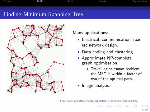
Finding Minimum Spanning Tree
Many applications:
• Electrical, communication, roadetc network design.
• Data coding and clustering.
• Approximate NP-completegraph optimisation.• Travelling salesman problem:
the MST is within a factor oftwo of the optimal path.
• Image analysis.
http://www.geeksforgeeks.org/applications-of-minimum-spanning-tree/
4 / 60

Outline MST Prim Kruskal Optimisation
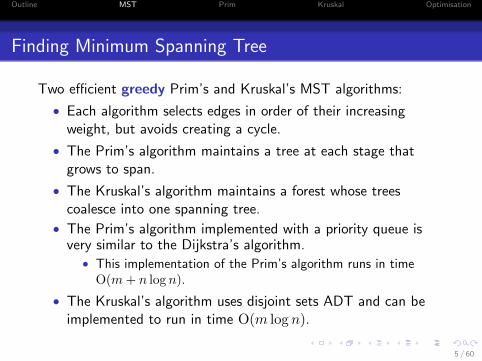
Finding Minimum Spanning Tree
Two efficient greedy Prim’s and Kruskal’s MST algorithms:
• Each algorithm selects edges in order of their increasingweight, but avoids creating a cycle.
• The Prim’s algorithm maintains a tree at each stage thatgrows to span.
• The Kruskal’s algorithm maintains a forest whose treescoalesce into one spanning tree.
• The Prim’s algorithm implemented with a priority queue isvery similar to the Dijkstra’s algorithm.• This implementation of the Prim’s algorithm runs in time
O(m+ n log n).
• The Kruskal’s algorithm uses disjoint sets ADT and can beimplemented to run in time O(m log n).
5 / 60

Outline MST Prim Kruskal Optimisation
Finding Minimum Spanning Tree
Two efficient greedy Prim’s and Kruskal’s MST algorithms:
• Each algorithm selects edges in order of their increasingweight, but avoids creating a cycle.
• The Prim’s algorithm maintains a tree at each stage thatgrows to span.
• The Kruskal’s algorithm maintains a forest whose treescoalesce into one spanning tree.
• The Prim’s algorithm implemented with a priority queue isvery similar to the Dijkstra’s algorithm.• This implementation of the Prim’s algorithm runs in time
O(m+ n log n).
• The Kruskal’s algorithm uses disjoint sets ADT and can beimplemented to run in time O(m log n).
5 / 60

Outline MST Prim Kruskal Optimisation
Prim’s MST Algorithm
algorithm Prim( weighted graph (G, c), vertex s )array w[n] = {c[s, 0], c[s, 1], . . . , c[s, n− 1]}S ← {s} first vertex added to MSTwhile S 6= V (G) do
find u ∈ V (G) \ S so that w[u] is minimum
S ← S ∪ {u} adding an edge adjacent to u to MST
for x ∈ V (G) \ S dow[x]← min{w[x], c[u, x]}
end forend while
Very similar to the Dijkstra’s algorithm:
• Priority queue should be used for selecting the lowest edge weights w[. . .].
• In the priority queue implementation, most time is taken byEXTRACT-MIN and DECREASE-KEY operations.
6 / 60

Outline MST Prim Kruskal Optimisation
Illustrating the Prim’s Algorithm
a bc
d
f
g
h
i j
1
4
6
5
2
2
9
8
12
13
8
15
13
7
1
5
10
S ={a}
w =a b c d f g h i j0 1 ∞ 8 ∞ ∞ 2 ∞ ∞
7 / 60

Outline MST Prim Kruskal Optimisation
Illustrating the Prim’s Algorithm
a bc
d
f
g
h
i j
1
4
6
5
2
2
9
8
12
13
8
15
13
7
1
5
10
S ={a,b}
w =a b c d f g h i j0 1a 13b 8a 5b ∞ 2a ∞ ∞
7 / 60

Outline MST Prim Kruskal Optimisation
Illustrating the Prim’s Algorithm
a bc
d
f
g
h
i j
1
4
6
5
2
2
9
8
12
13
8
15
13
7
1
5
10
S ={a,b,h
}w =
a b c d f g h i j0 1a 13b 5h 5b ∞ 2a 9h ∞
7 / 60

Outline MST Prim Kruskal Optimisation
Illustrating the Prim’s Algorithm
a bc
d
f
g
h
i j
1
4
6
5
2
2
9
8
12
13
8
15
13
7
1
5
10
S ={a,b,d,h
}w =
a b c d f g h i j0 1a 13b 5h 5b ∞ 2a 1d ∞
7 / 60

Outline MST Prim Kruskal Optimisation
Illustrating the Prim’s Algorithm
a bc
d
f
g
h
i j
1
4
6
5
2
2
9
8
12
13
8
15
13
7
1
5
10
S ={a,b,d,h,i
}w =
a b c d f g h i j0 1a 13b 5h 5b ∞ 2a 1d 12i
7 / 60

Outline MST Prim Kruskal Optimisation
Illustrating the Prim’s Algorithm
a bc
d
f
g
h
i j
1
4
6
5
2
2
9
8
12
13
8
15
13
7
1
5
10
S ={a,b,d,f,h,i
}w =
a b c d f g h i j0 1a 7f 5h 5b 13f 2a 1d 12i
7 / 60

Outline MST Prim Kruskal Optimisation
Illustrating the Prim’s Algorithm
a bc
d
f
g
h
i j
1
4
6
5
2
2
9
8
12
13
8
15
13
7
1
5
10
S ={a,b,c,d,f,h,i
}w =
a b c d f g h i j0 1a 7f 5h 5b 4c 2a 1d 12i
7 / 60

Outline MST Prim Kruskal Optimisation
Illustrating the Prim’s Algorithm
a bc
d
f
g
h
i j
1
4
6
5
2
2
9
8
12
13
8
15
13
7
1
5
10
S ={a,b,c,d,f,g,h,i
}w =
a b c d f g h i j0 1a 7f 5h 5b 4c 2a 1d 2g
7 / 60

Outline MST Prim Kruskal Optimisation
Illustrating the Prim’s Algorithm
a bc
d
f
g
h
i j
1
4
6
5
2
2
9
8
12
13
8
15
13
7
1
5
10
S ={a,b,c,d,f,g,h,i,j
}w =
a b c d f g h i j0 1a 7f 5h 5b 4c 2a 1d 2g
7 / 60

Outline MST Prim Kruskal Optimisation
Prim’s Algorithm (Priority Queue Implementation)
algorithm Prim (weighted graph (G, c), vertex s ∈ V (G) )priority queue Q, arrays colour[n], pred[n]for u ∈ V (G) do
pred[u]← NULL; colour[u]← WHITEend forcolour[s]← GREY; Q.insert(s, 0)while not Q.isEmpty() do
u← Q.peek()for each x adjacent to u do
t← c(u, x);if colour[x] = WHITE then
colour[x]← GREY; pred[x]← u; Q.insert(x, t)else if colour[x] = GREY and Q.getKey(x) > t then
Q.decreaseKey(x, t); pred[x]← uend if
end forQ.delete(); colour[u]← BLACK
end whilereturn pred
8 / 60
Outline MST Prim Kruskal Optimisation
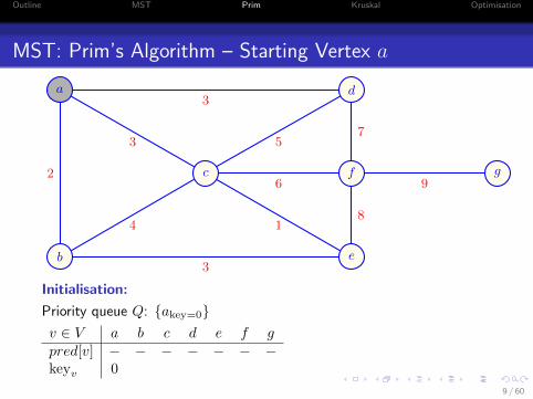
MST: Prim’s Algorithm – Starting Vertex a
2
4
3
3 5
6
1
7
8
9
3
b
a
c
e
f
d
g
Initialisation:
Priority queue Q: {akey=0}v ∈ V a b c d e f gpred[v] − − − − − − −keyv 0
9 / 60
Outline MST Prim Kruskal Optimisation
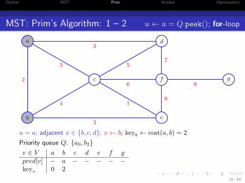
MST: Prim’s Algorithm: 1 – 2 u← a = Q.peek(); for-loop
2
4
3
3 5
6
1
7
8
9
3
b
a
c
e
f
d
g
u = a; adjacent x ∈ {b, c, d}; x← b; keyb ← cost(a, b) = 2
Priority queue Q: {a0, b2}v ∈ V a b c d e f gpred[v] − a − − − − −keyv 0 2
10 / 60

Outline MST Prim Kruskal Optimisation
MST: Prim’s Algorithm: 3 u = a; for-loop
2
4
3
3 5
6
1
7
8
9
3
b
a
c
e
f
d
g
adjacent x ∈ {b, c, d}; x← c; keyc ← cost(a, c) = 3
Priority queue Q: {a0, b2, c3}v ∈ V a b c d e f gpred[v] − a a − − − −keyv 0 2 3
11 / 60
Outline MST Prim Kruskal Optimisation
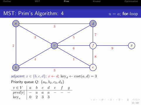
MST: Prim’s Algorithm: 4 u = a; for-loop
2
4
3
3 5
6
1
7
8
9
3
b
a
c
e
f
d
g
adjacent x ∈ {b, c, d}; x← d; keyd ← cost(a, d) = 3
Priority queue Q: {a0, b2, c3, d3}v ∈ V a b c d e f gpred[v] − a a a − − −keyv 0 2 3 3
12 / 60

Outline MST Prim Kruskal Optimisation
MST: Prim’s Algorithm: 5 – 6 Q.delete()
2
4
3
3 5
6
1
7
8
9
3
b
a
c
e
f
d
g
Q.delete() – excluding the vertex a
Priority queue Q: {b2, c3, d3}v ∈ V a b c d e f gpred[v] − a a a − − −keyv 0 2 3 3
13 / 60
Outline MST Prim Kruskal Optimisation
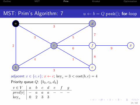
MST: Prim’s Algorithm: 7 u← b = Q.peek(); for-loop
2
4
3
3 5
6
1
7
8
9
3
b
a
c
e
f
d
g
adjacent x ∈ {c, e}; x← c; keyc = 3 < cost(b, c) = 4
Priority queue Q: {b2, c3, d3}v ∈ V a b c d e f gpred[v] − a a a − − −keyv 0 2 3 3
14 / 60
Outline MST Prim Kruskal Optimisation
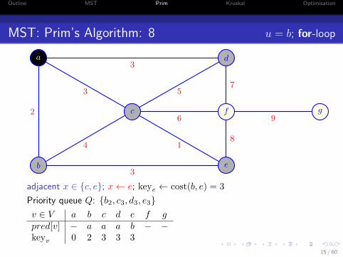
MST: Prim’s Algorithm: 8 u = b; for-loop
2
4
3
3 5
6
1
7
8
9
3
b
a
c
e
f
d
g
adjacent x ∈ {c, e}; x← e; keye ← cost(b, e) = 3
Priority queue Q: {b2, c3, d3, e3}v ∈ V a b c d e f gpred[v] − a a a b − −keyv 0 2 3 3 3
15 / 60

Outline MST Prim Kruskal Optimisation
MST: Prim’s Algorithm: 9 – 10 Q.delete()
2
4
3
3 5
6
1
7
8
9
3
b
a
c
e
f
d
g
Q.delete() – excluding the vertex b
Priority queue Q: {c3, d3, e3}v ∈ V a b c d e f gpred[v] − a a a b − −keyv 0 2 3 3 3
16 / 60
Outline MST Prim Kruskal Optimisation
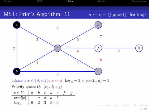
MST: Prim’s Algorithm: 11 u← c = Q.peek(); for-loop
2
4
3
3 5
6
1
7
8
9
3
b
a
c
e
f
d
g
adjacent x ∈ {d, e, f}; x← d; keyd = 3 < cost(c, d) = 5
Priority queue Q: {c3, d3, e3}v ∈ V a b c d e f gpred[v] − a a a b − −keyv 0 2 3 3 3
17 / 60

Outline MST Prim Kruskal Optimisation
MST: Prim’s Algorithm: 12 u = c; for-loop
2
4
3
3 5
6
1
7
8
9
3
b
a
c
e
f
d
g
adjacent x ∈ {d, e, f}; x← e; keye = 3 > cost(c, e) = 1; keye ← 1
Priority queue Q: {c3, d3, e1}v ∈ V a b c d e f gpred[v] − a a a c − −keyv 0 2 3 3 1
18 / 60
Outline MST Prim Kruskal Optimisation
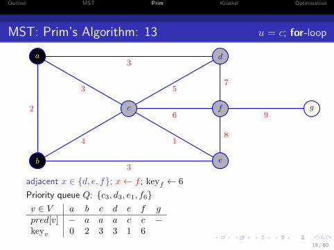
MST: Prim’s Algorithm: 13 u = c; for-loop
2
4
3
3 5
6
1
7
8
9
3
b
a
c
e
f
d
g
adjacent x ∈ {d, e, f}; x← f ; keyf ← 6
Priority queue Q: {c3, d3, e1, f6}v ∈ V a b c d e f gpred[v] − a a a c c −keyv 0 2 3 3 1 6
19 / 60

Outline MST Prim Kruskal Optimisation
MST: Prim’s Algorithm: 14 – 15 Q.delete()
2
4
3
3 5
6
1
7
8
9
3
b
a
c
e
f
d
g
Q.delete() – excluding the vertex c
Priority queue Q: {e1, d3, f6}v ∈ V a b c d e f gpred[v] − a a a c c −keyv 0 2 3 3 1 6
20 / 60

Outline MST Prim Kruskal Optimisation
MST: Prim’s Algorithm: 16 u← e = Q.peek(); for-loop
2
4
3
3 5
6
1
7
8
9
3
b
a
c
e
f
d
g
adjacent x ∈ {f}; x← f ; keyf ← 6 < cost(e, f) = 8
Priority queue Q: {e1, d3, f6}v ∈ V a b c d e f gpred[v] − a a a c c −keyv 0 2 3 3 1 6
21 / 60
Outline MST Prim Kruskal Optimisation
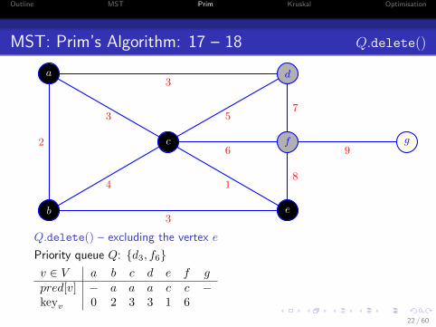
MST: Prim’s Algorithm: 17 – 18 Q.delete()
2
4
3
3 5
6
1
7
8
9
3
b
a
c
e
f
d
g
Q.delete() – excluding the vertex e
Priority queue Q: {d3, f6}v ∈ V a b c d e f gpred[v] − a a a c c −keyv 0 2 3 3 1 6
22 / 60

Outline MST Prim Kruskal Optimisation
MST: Prim’s Algorithm: 19 u← d = Q.peek(); for-loop
2
4
3
3 5
6
1
7
8
9
3
b
a
c
e
f
d
g
adjacent x ∈ {f}; x← f ; keyf ← 6 < cost(d, f) = 7
Priority queue Q: {d3, f6}v ∈ V a b c d e f gpred[v] − a a a c c −keyv 0 2 3 3 1 6
23 / 60

Outline MST Prim Kruskal Optimisation
MST: Prim’s Algorithm: 20 – 21 Q.delete()
2
4
3
3 5
6
1
7
8
9
3
b
a
c
e
f
d
g
Q.delete() – excluding the vertex d
Priority queue Q: {f6}v ∈ V a b c d e f gpred[v] − a a a c c −keyv 0 2 3 3 1 6
24 / 60
Outline MST Prim Kruskal Optimisation
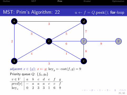
MST: Prim’s Algorithm: 22 u← f = Q.peek(); for-loop
2
4
3
3 5
6
1
7
8
9
3
b
a
c
e
f
d
g
adjacent x ∈ {g}; x← g; keyg ← cost(f, g) = 9
Priority queue Q: {f6, g9}v ∈ V a b c d e f gpred[v] − a a a c c fkeyv 0 2 3 3 1 6 9
25 / 60

Outline MST Prim Kruskal Optimisation
MST: Prim’s Algorithm: 23 Q.delete()
2
4
3
3 5
6
1
7
8
9
3
b
a
c
e
f
d
g
Q.delete() – excluding the vertex f
Priority queue Q: {g9}v ∈ V a b c d e f gpred[v] − a a a c c fkeyv 0 2 3 3 1 6 9
26 / 60
Outline MST Prim Kruskal Optimisation
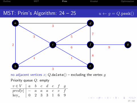
MST: Prim’s Algorithm: 24 – 25 u← g = Q.peek()
2
4
3
3 5
6
1
7
8
9
3
b
a
c
e
f
d
g
no adjacent vertices x; Q.delete() – excluding the vertex g
Priority queue Q: empty
v ∈ V a b c d e f gpred[v] − a a a c c fkeyv 0 2 3 3 1 6 9
27 / 60
Outline MST Prim Kruskal Optimisation
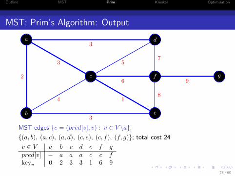
MST: Prim’s Algorithm: Output
2
4
3
3 5
6
1
7
8
9
3
b
a
c
e
f
d
g
MST edges {e = (pred[v], v) : v ∈ V \a}:{(a, b), (a, c), (a, d), (c, e), (c, f), (f, g)}; total cost 24
v ∈ V a b c d e f gpred[v] − a a a c c fkeyv 0 2 3 3 1 6 9
28 / 60

Outline MST Prim Kruskal Optimisation
Kruskal’s MST Algorithm
algorithm Kruskal( weighted graph (G, c) )T ← ∅insert E(G) into a priority queuefor e = {u, v} ∈ E(G) in increasing order of weight do
if u and v are not in the same tree thenT ← T ∪ {e}merge the trees of u and v
end ifend for
• Keeping track of the trees using the disjoint sets ADT, with standardoperations FIND and UNION.
• They can be implemented efficiently so that the main time taken is at thesorting step.
29 / 60

Outline MST Prim Kruskal Optimisation
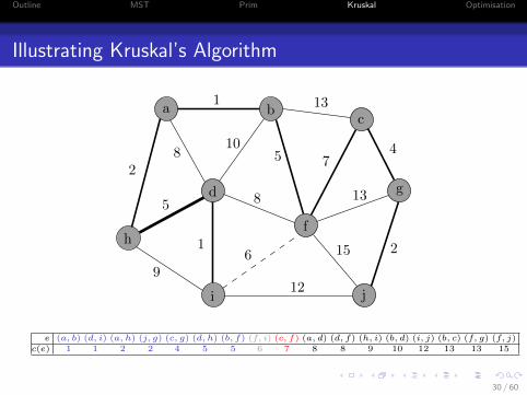
Illustrating Kruskal’s Algorithm
a bc
d
f
g
h
i j
1
4
6
5
2
2
9
8
12
13
8
15
13
7
1
5
10
e (a, b) (d, i) (a, h) (j, g) (c, g) (d, h) (b, f) (f, i) (c, f) (a, d) (d, f) (h, i) (b, d) (i, j) (b, c) (f, g) (f, j)c(e) 1 1 2 2 4 5 5 6 7 8 8 9 10 12 13 13 15
30 / 60

Outline MST Prim Kruskal Optimisation
Illustrating Kruskal’s Algorithm
a bc
d
f
g
h
i j
1
4
6
52
2
9
8
12
13
8
15
13
7
1
5
10
e (a, b) (d, i) (a, h) (j, g) (c, g) (d, h) (b, f) (f, i) (c, f) (a, d) (d, f) (h, i) (b, d) (i, j) (b, c) (f, g) (f, j)c(e) 1 1 2 2 4 5 5 6 7 8 8 9 10 12 13 13 15
30 / 60

Outline MST Prim Kruskal Optimisation
Illustrating Kruskal’s Algorithm
a bc
d
f
g
h
i j
1
4
6
52
2
9
8
12
13
8
15
13
7
1
5
10
e (a, b) (d, i) (a, h) (j, g) (c, g) (d, h) (b, f) (f, i) (c, f) (a, d) (d, f) (h, i) (b, d) (i, j) (b, c) (f, g) (f, j)c(e) 1 1 2 2 4 5 5 6 7 8 8 9 10 12 13 13 15
30 / 60

Outline MST Prim Kruskal Optimisation
Illustrating Kruskal’s Algorithm
a bc
d
f
g
h
i j
1
4
6
52
2
9
8
12
13
8
15
13
7
1
5
10
e (a, b) (d, i) (a, h) (j, g) (c, g) (d, h) (b, f) (f, i) (c, f) (a, d) (d, f) (h, i) (b, d) (i, j) (b, c) (f, g) (f, j)c(e) 1 1 2 2 4 5 5 6 7 8 8 9 10 12 13 13 15
30 / 60

Outline MST Prim Kruskal Optimisation
Illustrating Kruskal’s Algorithm
a bc
d
f
g
h
i j
1
4
6
52
2
9
8
12
13
8
15
13
7
1
5
10
e (a, b) (d, i) (a, h) (j, g) (c, g) (d, h) (b, f) (f, i) (c, f) (a, d) (d, f) (h, i) (b, d) (i, j) (b, c) (f, g) (f, j)c(e) 1 1 2 2 4 5 5 6 7 8 8 9 10 12 13 13 15
30 / 60

Outline MST Prim Kruskal Optimisation
Illustrating Kruskal’s Algorithm
a bc
d
f
g
h
i j
1
4
6
52
2
9
8
12
13
8
15
13
7
1
5
10
e (a, b) (d, i) (a, h) (j, g) (c, g) (d, h) (b, f) (f, i) (c, f) (a, d) (d, f) (h, i) (b, d) (i, j) (b, c) (f, g) (f, j)c(e) 1 1 2 2 4 5 5 6 7 8 8 9 10 12 13 13 15
30 / 60
Outline MST Prim Kruskal Optimisation
Illustrating Kruskal’s Algorithm
a bc
d
f
g
h
i j
1
4
6
52
2
9
8
12
13
8
15
13
7
1
5
10
e (a, b) (d, i) (a, h) (j, g) (c, g) (d, h) (b, f) (f, i) (c, f) (a, d) (d, f) (h, i) (b, d) (i, j) (b, c) (f, g) (f, j)c(e) 1 1 2 2 4 5 5 6 7 8 8 9 10 12 13 13 15
30 / 60

Outline MST Prim Kruskal Optimisation
MST: Kruskal’s Algorithm
2
4
3
3 5
6
1
7
8
9
3
b
a
c
e
f
d
g
Initialisation:
Disjoint-sets ADT A ={{a}, {b}, {c}, {d}, {e}, {f}, {g}
}cost 1 2 3 3 3 4 5 6 7 8 9edge (c, e) (a, b) (a, c) (a, d) (b, e) (b, c) (c, d) (c, f) (d, f) (e, f) (f, g)
31 / 60
Outline MST Prim Kruskal Optimisation
MST: Kruskal’s Algorithm 1
2
4
3
3 5
6
1
7
8
9
3
b
a
c
e
f
d
g
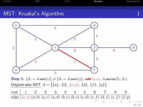
Step 1: {Sc = A.set(c)} 6= {Se = A.set(e)}; add (c, e); A.union(Sc, Se)
Disjoint-sets ADT A ={{a}, {b}, {c, e}, {d}, {f}, {g}
}cost 1 2 3 3 3 4 5 6 7 8 9edge (c, e) (a, b) (a, c) (a, d) (b, e) (b, c) (c, d) (c, f) (d, f) (e, f) (f, g)
32 / 60
Outline MST Prim Kruskal Optimisation
MST: Kruskal’s Algorithm 2
2
4
3
3 5
6
1
7
8
9
3
b
a
c
e
f
d
g
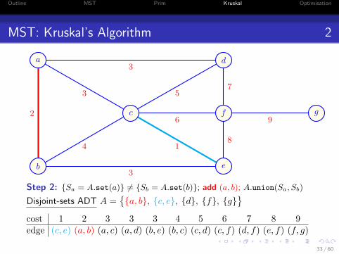
Step 2: {Sa = A.set(a)} 6= {Sb = A.set(b)}; add (a, b); A.union(Sa, Sb)
Disjoint-sets ADT A ={{a, b}, {c, e}, {d}, {f}, {g}
}cost 1 2 3 3 3 4 5 6 7 8 9edge (c, e) (a, b) (a, c) (a, d) (b, e) (b, c) (c, d) (c, f) (d, f) (e, f) (f, g)
33 / 60

Outline MST Prim Kruskal Optimisation
MST: Kruskal’s Algorithm 3
2
4
3
3 5
6
1
7
8
9
3
b
a
c
e
f
d
g
Step 3: {Sa = A.set(a)} 6= {Sc = A.set(c)}; add (a, c); A.union(Sa, Sc)
Disjoint-sets ADT A ={{a, b, c, e}, {d}, {f}, {g}
}cost 1 2 3 3 3 4 5 6 7 8 9edge (c, e) (a, b) (a, c) (a, d) (b, e) (b, c) (c, d) (c, f) (d, f) (e, f) (f, g)
34 / 60
Outline MST Prim Kruskal Optimisation
MST: Kruskal’s Algorithm 4
2
4
3
3 5
6
1
7
8
9
3
b
a
c
e
f
d
g
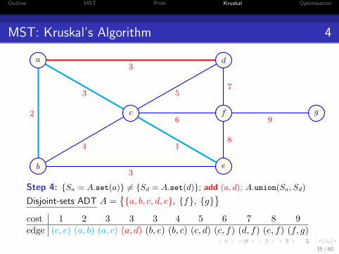
Step 4: {Sa = A.set(a)} 6= {Sd = A.set(d)}; add (a, d); A.union(Sa, Sd)
Disjoint-sets ADT A ={{a, b, c, d, e}, {f}, {g}
}cost 1 2 3 3 3 4 5 6 7 8 9edge (c, e) (a, b) (a, c) (a, d) (b, e) (b, c) (c, d) (c, f) (d, f) (e, f) (f, g)
35 / 60

Outline MST Prim Kruskal Optimisation
MST: Kruskal’s Algorithm 5
2
4
3
3 5
6
1
7
8
9
3
b
a
c
e
f
d
g
Step 5: {Sb = A.set(b)} = {Se = A.set(e)}; skip (b, e)
Disjoint-sets ADT A ={{a, b, c, d, e}, {f}, {g}
}cost 1 2 3 3 3 4 5 6 7 8 9edge (c, e) (a, b) (a, c) (a, d) (b, e) (b, c) (c, d) (c, f) (d, f) (e, f) (f, g)
36 / 60
Outline MST Prim Kruskal Optimisation
MST: Kruskal’s Algorithm 6
2
4
3
3 5
6
1
7
8
9
3
b
a
c
e
f
d
g
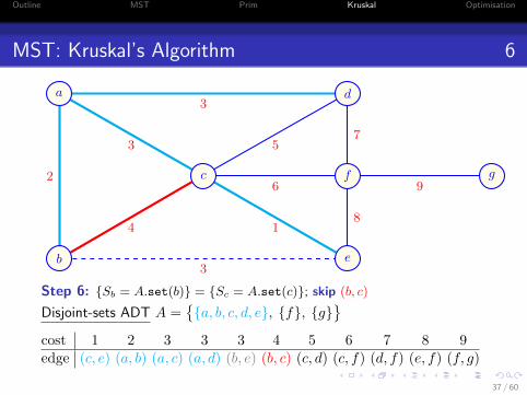
Step 6: {Sb = A.set(b)} = {Sc = A.set(c)}; skip (b, c)
Disjoint-sets ADT A ={{a, b, c, d, e}, {f}, {g}
}cost 1 2 3 3 3 4 5 6 7 8 9edge (c, e) (a, b) (a, c) (a, d) (b, e) (b, c) (c, d) (c, f) (d, f) (e, f) (f, g)
37 / 60
Outline MST Prim Kruskal Optimisation
MST: Kruskal’s Algorithm 7
2
4
3
3 5
6
1
7
8
9
3
b
a
c
e
f
d
g
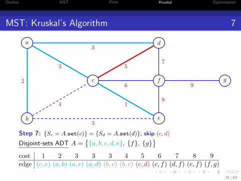
Step 7: {Sc = A.set(c)} = {Sd = A.set(d)}; skip (c, d)
Disjoint-sets ADT A ={{a, b, c, d, e}, {f}, {g}
}cost 1 2 3 3 3 4 5 6 7 8 9edge (c, e) (a, b) (a, c) (a, d) (b, e) (b, c) (c, d) (c, f) (d, f) (e, f) (f, g)
38 / 60

Outline MST Prim Kruskal Optimisation
MST: Kruskal’s Algorithm 8
2
4
3
3 5
6
1
7
8
9
3
b
a
c
e
f
d
g
Step 8: {Sc = A.set(c)} 6= {Sf = A.set(f)}; add (c, f); A.union(Sc, Sf )
Disjoint-sets ADT A ={{a, b, c, d, e, f}, {g}
}cost 1 2 3 3 3 4 5 6 7 8 9edge (c, e) (a, b) (a, c) (a, d) (b, e) (b, c) (c, d) (c, f) (d, f) (e, f) (f, g)
39 / 60

Outline MST Prim Kruskal Optimisation
MST: Kruskal’s Algorithm 9
2
4
3
3 5
6
1
7
8
9
3
b
a
c
e
f
d
g
Step 9: {Sd = A.set(d)} = {Sf = A.set(f)}; skip (d, f)
Disjoint-sets ADT A ={{a, b, c, d, e, f}, {g}
}cost 1 2 3 3 3 4 5 6 7 8 9edge (c, e) (a, b) (a, c) (a, d) (b, e) (b, c) (c, d) (c, f) (d, f) (e, f) (f, g)
40 / 60
Outline MST Prim Kruskal Optimisation
MST: Kruskal’s Algorithm 10
2
4
3
3 5
6
1
7
8
9
3
b
a
c
e
f
d
g
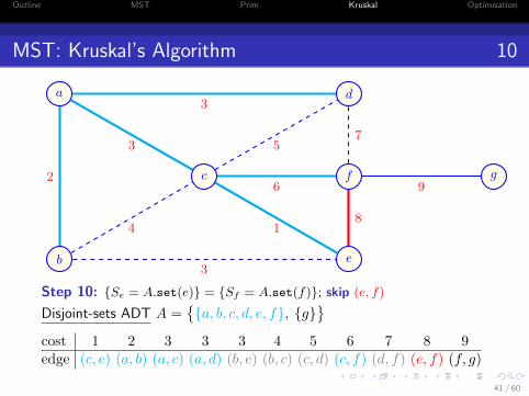
Step 10: {Se = A.set(e)} = {Sf = A.set(f)}; skip (e, f)
Disjoint-sets ADT A ={{a, b, c, d, e, f}, {g}
}cost 1 2 3 3 3 4 5 6 7 8 9edge (c, e) (a, b) (a, c) (a, d) (b, e) (b, c) (c, d) (c, f) (d, f) (e, f) (f, g)
41 / 60

Outline MST Prim Kruskal Optimisation
MST: Kruskal’s Algorithm 11
2
4
3
3 5
6
1
7
8
9
3
b
a
c
e
f
d
g
Step 11: {Sf = A.set(f)} 6= {Sg = A.set(g)}; add (f, g); A.union(Sf , Sg)
Disjoint-sets ADT A ={{a, b, c, d, e, f, g}
}cost 1 2 3 3 3 4 5 6 7 8 9edge (c, e) (a, b) (a, c) (a, d) (b, e) (b, c) (c, d) (c, f) (d, f) (e, f) (f, g)
42 / 60

Outline MST Prim Kruskal Optimisation
MST: Kruskal’s Algorithm: Output
2
4
3
3 5
6
1
7
8
9
3
b
a
c
e
f
d
g
Step 11: {Sf = A.set(f)} 6= {Sg = A.set(g)}; add (f, g); A.union(Sf , Sg)
Disjoint-sets ADT A ={{a, b, c, d, e, f, g}
}cost 1 2 3 3 3 4 5 6 7 8 9edge (c, e) (a, b) (a, c) (a, d) (b, e) (b, c) (c, d) (c, f) (d, f) (e, f) (f, g)
43 / 60

Outline MST Prim Kruskal Optimisation
Comparing the Prim’s and Kruskal’s Algorithms
Both algorithms choose and add at each step a min-weight edgefrom the remaining edges, subject to constraints.
Prim’s MST algorithm:
• Start at a root vertex.
• Two rules for a new edge:
(a) No cycle in the subgraphbuilt so far.
(b) The connected subgraphbuilt so far.
• Terminate if no more edgesto add can be found.
At each step: an acyclicconnected subgraph being a tree.
Kruskal’s MST algorithm:
• Start at a min-weight edge.
• One rule for a new edge:
(a) No cycle in a forest oftrees built so far.
• Terminate if no more edgesto add can be found.
At each step: a forest of treesmerging as the algorithmprogresses (can find a spanning forest
for a disconnected graph).
44 / 60

Outline MST Prim Kruskal Optimisation
Correctness of Prim’s and Kruskal’s Algorithms
Theorem 6.15: Prim’s and Kruskal’s algorithms are correct.
• A set of edges is promising if it can be extended to a MST.
• The theorem claims that both the algorithms
1 choose at each step a promising set of edges and2 terminate with the MST as the set cannot be further extended.
Technical fact for proving these claims.
• Let B ⊂ V (G); |B| < n, be a proper subset of the vertices.
• Let T ⊂ E be a promising set of edges, such that no edge in Tleaves B (i.e., If (u, v) ∈ T , then either both u, v ∈ B or both u, v /∈ B).
• If a minimum-weight edge e leaves B (one endpoint in B and oneoutside), then the set T
⋃{e} is also promising.
45 / 60
Outline MST Prim Kruskal Optimisation
Correctness of Prim’s and Kruskal’s Algorithms
Proof of the technical fact that the set T⋃{e} is promising.
• Since the set T is promising, it is in a some MST U .
• If e ∈ U , there is nothing to prove.
• Otherwise, adding e to U creates exactly one cycle.• This cycle contains at least one more edge, e′, leaving B, as
otherwise the cycle could not close.
• Removing the edge e′ forms for the graph G a new spanningtree U ′.
• Its total weight is no greater than the total weight of theMST U , and thus the tree U ′ is also an MST.
• Since the MST U ′ contains the set T⋃{e} of edges, that set
is promising.
46 / 60

Outline MST Prim Kruskal Optimisation
Correctness of Prim’s and Kruskal’s Algorithms
V
B e = (u, v) /∈ T
e′
Proof of Theorem 6.15:
• Suppose that the MST algorithm has maintained a promisingset T of edges so far.
• Let an edge e = {u, v} have been just chosen.
• Let B denote at each step• either the set of vertices in the tree (Prim)• or in the tree containing the vertex u (Kruskal).
• Then the above technical fact can be applied to conclude thatT⋃{e} is promising and the algorithm is correct.
47 / 60

Outline MST Prim Kruskal Optimisation
Minimum Spanning Trees (MST): Some Properties
Can you prove these two facts?
1 The maximum-cost edge, if unique, of a cycle in an edge-weighted graph G is not in any MST.
Otherwise, at least one of those equally expensive edges of thecycle must not be in each MST.
2 The minimum-cost edge, if unique, between any non-emptystrict subset S of V (G) and the V (G) \ S is in any MST.
Otherwise, at least one of these minimum-cost edges must bein each MST.
Hint: Look whether a total weight of an MST with such a maximum-cost
edge or without such a minimum-cost edge can be further decreased.
48 / 60

Outline MST Prim Kruskal Optimisation
Other (Di)graph Optimisation/Decision Problems
There are many more graph and network computational andoptimisation problems.
Many of them do not have easy or polynomial-time solutions.
However, a few of them are in a special class in that their solutionscan be verified in polynomial time.
• This class of computational problems is called the NP(nondeterministic polynomial) class.
• In addition, many of these are proven to be harder thananything else in the NP class.
• The latter NP problems are called NP-complete ones.
Other algorithm design techniques like backtracking, branch-and-bound or approximation algorithms (studied in COMPSCI 320) areneeded.
49 / 60
Outline MST Prim Kruskal Optimisation
Examples of NP-complete Graph Problems
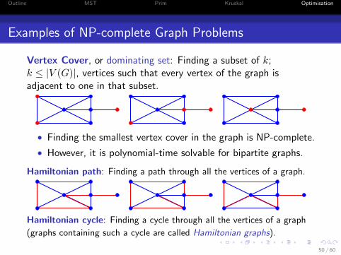
Vertex Cover, or dominating set: Finding a subset of k;k ≤ |V (G)|, vertices such that every vertex of the graph isadjacent to one in that subset.
• Finding the smallest vertex cover in the graph is NP-complete.
• However, it is polynomial-time solvable for bipartite graphs.
Hamiltonian path: Finding a path through all the vertices of a graph.
Hamiltonian cycle: Finding a cycle through all the vertices of a graph
(graphs containing such a cycle are called Hamiltonian graphs).
50 / 60

Outline MST Prim Kruskal Optimisation
Hamiltonian Paths - Exampleshttp://www.cs.utsa.edu/~wagner/CS3343/graphapp2/hampaths.html
The longest (18,040 miles) Hamiltonian path from Maine (ME) between capitals of all48 mainland US states out of the 68, 656, 026 possible Hamiltonian paths:
51 / 60

Outline MST Prim Kruskal Optimisation
Hamiltonian Paths - Exampleshttp://www.cs.utsa.edu/~wagner/CS3343/graphapp2/hampaths.html
The random (13,619miles) Hamiltonian path from Maine (ME) between capitals of all48 mainland US states out of the 68, 656, 026 possible Hamiltonian paths:
52 / 60

Outline MST Prim Kruskal Optimisation
Hamiltonian Paths - Exampleshttp://www.cs.utsa.edu/~wagner/CS3343/graphapp2/hampaths.html
The shortest (11,698 miles) Hamiltonian path from Maine (ME) between capitals ofall 48 mainland US states out of the 68, 656, 026 possible Hamiltonian paths:
53 / 60
Outline MST Prim Kruskal Optimisation
Examples of NP-complete Graph Problems
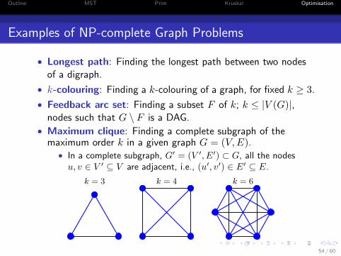
• Longest path: Finding the longest path between two nodesof a digraph.
• k-colouring: Finding a k-colouring of a graph, for fixed k ≥ 3.
• Feedback arc set: Finding a subset F of k; k ≤ |V (G)|,nodes such that G \ F is a DAG.
• Maximum clique: Finding a complete subgraph of themaximum order k in a given graph G = (V,E).• In a complete subgraph, G′ = (V ′, E′) ⊂ G, all the nodes
u, v ∈ V ′ ⊆ V are adjacent, i.e., (u′, v′) ∈ E′ ⊆ E.
k = 3 k = 4 k = 6
54 / 60

Outline MST Prim Kruskal Optimisation
NP-complete Graph Colouring: Examples
https://en.wikipedia.org/wiki/Graph_coloring
http://iasbs.ac.ir/seminar/math/combinatorics/
https://heuristicswiki.wikispaces.com/Graph+coloring
Optimisation: Colouring a general graph with the minimum number of colours.
Greedy colouring
55 / 60
Outline MST Prim Kruskal Optimisation
Examples of NP-complete Graph Problems
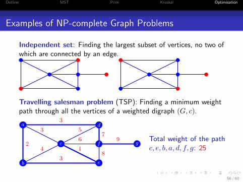
Independent set: Finding the largest subset of vertices, no two ofwhich are connected by an edge.
Travelling salesman problem (TSP): Finding a minimum weightpath through all the vertices of a weighted digraph (G, c).
38
7
3
24
53
1
6 9
b
a
c
e
f
d
gTotal weight of the pathc, e, b, a, d, f, g: 25
56 / 60

Outline MST Prim Kruskal Optimisation
TSP – NP-Hard, but not NP-Complete Problem
Blog by Jean Francois Paget: https://www.ibm.com/developerworks/community/
blogs/jfp/entry/no_the_tsp_isn_t_np_complete?lang=en
• NP problem – its solution can be verified in polynomial time.
• NP-hard problem – it is as difficult as any NP problem.
• NP-complete problem – it is both NP and NP-hard.
For a given TSP solution:
1 Each city is visited once (easy verified in polynomial time).
2 Total travel length is minimal (no known polynomial-time check).
Nn = (n− 1)! of paths through n vertices, starting from an arbitrary vertex:
n 10 20 100 1000 10000
Nn 3.63 · 105 1.22 · 1017 9.33 · 155 4.02 · 102564 2.85 · 1035655
57 / 60

Outline MST Prim Kruskal Optimisation
TSP – NP-Hard, but not NP-Complete Problem
Blog by Jean Francois Paget: https://www.ibm.com/developerworks/community/
blogs/jfp/entry/no_the_tsp_isn_t_np_complete?lang=en
Effective algorithms for solving the TSPs with large n exist. See, e.g., theoptimal TSP solution by D. Applegate, R. Bixby, V. Chvatal, and W. Cook forn = 13, 509 cities and towns with more than 500 residents in the USA:
58 / 60
Outline MST Prim Kruskal Optimisation
Examples of NP-complete Graph Problems
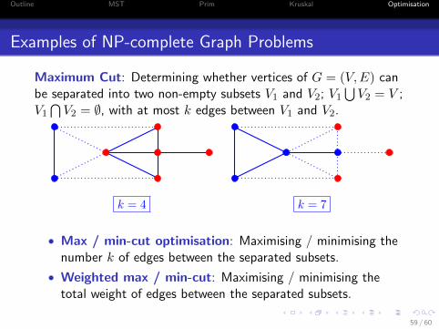
Maximum Cut: Determining whether vertices of G = (V,E) canbe separated into two non-empty subsets V1 and V2; V1
⋃V2 = V ;
V1⋂
V2 = ∅, with at most k edges between V1 and V2.
k = 4 k = 7
• Max / min-cut optimisation: Maximising / minimising thenumber k of edges between the separated subsets.
• Weighted max / min-cut: Maximising / minimising thetotal weight of edges between the separated subsets.
59 / 60

Outline MST Prim Kruskal Optimisation
Examples of NP-complete Graph Problems
• Induced path: Determining whether there is an inducedsubgraph of order k being a simple path.
• Bandwidth: Determining whether there is a linear ordering ofV with bandwidth k or less.• Bandwidth k – each edge spans at most k vertices.
• Subgraph Isomorphism: Determining whether H is asub(di)graph of G.
• Minimum broadcast time: Determining for a given sourcenode of a digraph G, whether (point-to-point) broadcast to allother nodes can take at most k time steps.
• Disjoint connecting paths: Determining for given k pairs ofsource and sink vertices of a graph G, whether there are kvertex-disjoint paths connecting each pair.
60 / 60
Recommended