Private Labels and Retailer Profitability:Bilateral Bargaining in the Grocery Channel∗
Paul B. Ellicksona, Pianpian Kongb, and Mitchell J. Lovetta
aSimon Business School, University of RochesterbSchool of Management, University at Buffalo, SUNY
September 29, 2017
Abstract
We examine the role of store branded “private label” products in determining bar-gaining outcomes between retailers and manufacturers in the single-serve brew-at-homecoffee category. Exploiting a novel setting in which the dominant, single-serve technol-ogy was protected by a patent that prevented private label entry, we develop a struc-tural model of demand and supply-side bargaining and seek to quantify the impact ofprivate labels on retailer profits. To quantify the benefits of private label introduction,we decompose their impact into the direct profits (from adding an additional product)and the bargaining benefit on branded products (from increasing retailer’s bargainingleverage), netting out the business stealing effects on incumbent branded products.We find that bargaining outcomes are driven primarily by bargaining leverage, whilebargaining ability is relatively symmetric between retailer and manufacturer. More-over, the impact of bargaining leverage is substantial: increased bargaining leverageaccounts for roughly 20% of the overall benefit of private label introduction, whichis itself on the order of 10% of pre-introduction profits. Finally, we find that privatelabels are beneficial to all retailers, but some retailers gain much more than others.
Keywords: Retail Grocery, Bargaining Models, Private Labels, Store Brands, De-mand Estimation.
∗We thank Guy Arie, Greg Crawford, Michaela Draganska, Ron Goettler, Paul Grieco and Ali Yu-rukoglu for valuable comments. We also thank seminar participants at Arizona State Carey, DukeFuqua, Goethe Universitat, Houston, Northwestern Kellogg, Penn State economics, University of Rochester,Simon Business School, Yale SOM and the University of Zurich as well as attendees at INFORMSMarketing Science 2017, SICS 2017, and QME 2017 for helpful feedback. Send any correspondenceto [email protected] (Ellickson), [email protected] (Lovett) [email protected] (Kong).
1
1 Introduction
Private labels are an important source of retailer revenues and profits. They generated $98
billion in U.S. food and grocery sales in 2012, or 17.1% of total revenues (Schultz, 2012;
Nielsen Global Survey, 2012). The impact of private label brands on retailer category profits
can come directly from the private label sales themselves or indirectly through improved
negotiating positions with national brands. Direct profits increase because private labels can
attract new consumers or larger spending through lower prices; higher margins are another
benefit. Indirect profits arise because the store brand can play a strategic role in negotiations
with manufacturers and increase the retailers’ share of channel profits (Scott Morton and
Zettelmeyer, 2004). A private label improves the retailer’s bargaining position by reducing
the forgone profits if negotiations with manufacturers fail, generating a bargaining benefit
via more favorable margins on the competing branded products.1
In this paper, we measure the influence of private label entry on bargaining outcomes in
the single-cup brew-at-home coffee category and compare the size of the bargaining benefit to
that of the direct profit from simply adding more options. Our empirical analysis exploits a
unique setting in which the dominant branded product, Keurig/GMCR’s ‘K-Cup’ technology,
was patent protected, effectively preventing entry by private label coffee products prior to
patent expiration. Therefore, we are able to observe how retailers and manufacturers behave
both with and without competition from private label products, and isolate the factors that
change this conduct. Further, because our data contains many retailers, we observe variation
in the quality and positioning of the various private label brands. After the patent expiration,
this yields exogenous variation in the shock to negotiations that different retailers receive. To
leverage this unique source of variation, we build a model of consumer demand and supply-
side bargaining in the brew-at-home coffee category. We estimate the model using weekly,
chain-level data from 72 retail market areas. We then conduct counterfactual exercises
1A third benefit argued for store brands is store or store brand loyalty that increases traffic to the store.Our data limits our ability to speak to this potential benefit and so, beyond effects through changes in thedraw from the outside good, we do not claim to capture such benefits in this study.
2
that quantify the impact of private label products on bargaining outcomes, comparing the
bargaining benefit to the direct category expansion benefit of introducing private labels.
As noted above, our empirical strategy involves exploiting a unique setting that unfolded
in the brew-at-home coffee market over our sample period. A previously mature product
category, the brew-at-home coffee market was disrupted in the mid-to-late 2000s by a new
product offering: single-serving coffee pods. This new technology offered convenience, and
a standardized, high-quality brewing experience, to a growing segment of coffee connois-
seurs. While single-serve coffee had existed both in the U.S. and abroad for many years,
Keurig/GMCR was able to position itself as the de facto U.S. standard by offering a wide
range of sub-brands and licensed/partner products, alongside a design that was superior to
its rivals and much wider product distribution.2 Notably, since both the Keurig brewers
and K-Cup pods were patented, competitive entry (to this particular design) was effectively
foreclosed until late 2012, creating a unique “before and after experiment.” To exploit this
exclusion, we develop a structural model of demand and supply that can control for con-
founding factors in the competitive environment (e.g., cost changes, new product entries,
continued market expansion, and evolving substitution patterns) and reveal how private
labels shaped bargaining outcomes.
While providing a unique setting for analyzing private label competition, the single-
serve coffee category presents some challenges on the demand side. First, a central aspect
of the Keurig/GMCR strategy was brand variety, so it will be important to include the
full set of brands offered. Second, since this was a new product launch (that we observe
almost from inception), availability of K-Cup products was limited, especially in the early
periods. Finally, brewing single-cup pods requires owning relatively expensive and specialized
hardware (i.e., the Keurig brewer). Consumers that did not own the brewer were not in the
market for single-cup pods. Ignoring these market features could lead to large biases in our
2Keurig/GMCR is also the “category captain” in many retailers, adding to its dominant position (Nijset al., 2013). The category captain coordinates with the retailer to manage the selection and display of agiven product category. It is typically one of the leading national brands.
3
demand estimates. Getting the demand system right is critical, as it drives all subsequent
inference. We address all three concerns by extending Bruno and Vilcassim (2008) and
developing a random-coefficient, discrete-choice demand system that accounts for availability
and machine ownership by simulating individual consumers and aggregating up to observed
shares (availability and ownership are tied to the data via aggregate moments of each). We
demonstrate that the model yields flexible substitution patterns that capture key market
features, including substitution between single-cup products and variation in the private
label brand equities.
Turning to the supply side, we must first recover wholesale prices, as these are not
observed in the data. To do so, we assume monopolist retailers and use the first order
conditions from the retailer’s profit maximization problem to solve for the wholesale prices
that rationalize retailer decisions (Bresnahan, 1987; Werden and Froeb, 1994). We find that
these recovered wholesale prices decline in the period after the patent expiration as one
would expect if the bargaining benefit were meaningful.
These inferred wholesale prices are then the focus of our bargaining model. We assume
that retailers and manufacturers bargain over linear contracts that determine these “transfer
prices.” Following the recent literature, we model the retailer-manufacturer vertical contract-
ing relationship as a ‘Nash in Nash’ bargain, focused on determining the wholesale price that
effectively splits the gains from trade. Using the inferred wholesale prices, we recover the
bargaining power (ability) parameters and manufacturer cost parameters that rationalize
the data. To do so, we compute both the profits that each party achieves under agreement
and the profits that would obtain should they fail to reach agreement. The observed whole-
sale prices maximize the Nash product, as indexed by the power parameters. Private label
products provide a key source of variation in the disagreement payoffs that define the gains
from trade.
To estimate this bargaining model, we modify the empirical approach developed by
Grennan (2013), which allows us to recover separate bargaining parameters for each re-
4

tailer/manufacturer pair. We find that bargaining ability is quite symmetric between re-
tailers and manufacturers and also does not change significantly after the patent expiration
(private label entry). Thus, we find that bargaining outcomes are driven primarily by the
shift in bargaining leverage (position) that private labels create. We then conduct coun-
terfactual exercises that quantify their impact bargaining outcomes. The impact of the
change in bargaining leverage is substantial: bargaining benefits account for roughly 20%
of the overall benefit of private label introduction, which is itself on the order of 10% of
pre-introduction profits. We find that private labels are beneficial to all retailers, but some
retailers gain much more than others. The size of the gain increases with the quality of the
adjacent private label, suggesting that success in one category can be leveraged in others.
Our research relates to several streams of literature in both marketing and economics.
First, we contribute to the literature on private labels, which includes seminal papers by Hoch
and Banerji (1993) and Dhar and Hoch (1997) that identified and cataloged the determinants
of private label success, and sought to explain why their penetration varied across retailers.
Hansen et al. (2006) investigate whether consumer tastes for store brands are correlated
across categories, or are driven more by category-specific factors. They find strong evidence of
the former relative to the latter. Sayman et al. (2002) study how private labels are positioned
vis-a-vis national brands, and Scott Morton and Zettelmeyer (2004) show how private labels
allow the retailer to carry closer substitutes to national brands than otherwise and that this
arises because of the incentives national brands face in negotiating with retailers.
A few papers have studied questions more directly related to the bargaining benefit of
private labels per se. Pauwels and Srinivasan (2004) examine the impact of store brand
entry on the relative margins of retailers and suppliers, as well as their role in shifting
consumer demand. They examine four categories in the Dominick’s Finer Foods retail chain
and find that retailer margins improve, but that category sales only rarely expand upon
store brand entry. Similarly using Dominick’s data on the oats category, Chintagunta et al.
(2002) empirically analyze how private labels change conduct in the channel, as well as
5

how this conduct translates through to retailer pricing decisions. They find that post entry
manufacturers’ accommodate so that Dominick’s average weekly margin increased by around
3%, but that consumers tastes do not change post entry. Meza and Sudhir (2010) again use
Dominick’s data, but for the breakfast cereal market, and examine how private labels affect
bargaining power, and ask whether and how retailers can use prices to strategically influence
this negotiation. They find that bargaining power increases as evidenced by lower wholesale
prices on imitated national brands, but that strategic pricing is less clearly evidenced in
the data. We add to this literature along three key dimensions. First, our setting lets
exploit the patent expiration to evaluate behavior with and without exogenous private label
exclusion. Second, we implement a full bargaining model specification that allows us to
generate counterfactuals to investigate the causal effects of private labels and isolate the
bargaining component of the private label benefit. Third, we expand the investigation from
a single retailer to 54 different retailer banners and 72 different retail market areas, allowing
us to describe the distribution of private label bargaining and category expansion benefits
across varying private label brand qualities.
Our bargaining model draws upon the theoretical literature on bilateral Nash bargaining
(Nash, 1950; Rubinstein, 1982), which includes the theoretical development of the ‘Nash in
Nash’ bargaining solution for most applied work by Horn and Wolinsky (1988) and recent
developments by Collard-Wexler et al. (2014). In doing so, we contribute to the growing
stream of empirical literature on bargaining models, which includes papers by Misra and
Mohanty (2006), Ho (2009), Draganska et al. (2010), Crawford and Yurukoglu (2012), Gren-
nan (2013), Ho and Lee (2013), Gowrisankaran et al. (2014), and Crawford et al. (2015).
This work is also related to a broader empirical literature on vertical contracting, which in-
cludes important contributions by Villas-Boas (2007) and Bonnet and Dubois (2010), among
several others. Two papers in this literature on manufacturer-retailer relationships speak di-
rectly to the coffee market. Noton and Elberg (2016) model bargaining between retailers and
manufacturers in the Chilean market for instant and ground coffee, focusing on the impact of
6

supplier size on the split of channel profits. Contrary to conventional wisdom, they find that
small suppliers often attain shares of the channel surplus on par with the largest supplier.
In the paper most closely related to ours, Draganska et al. (2010) empirically model the bar-
gaining problem between retailers and manufactures in the German market for ground coffee,
seeking to quantify the sources of heterogeneous bargaining power and determine whether
they have shifted over time. They find that store brand entry, per se, does not increase
bargaining power, but that store brands positioned closer to national brands tend to have
stronger bargaining power. They also find that bargaining positioning has little impact on
profits.
Our contribution to the broader bargaining literature goes well beyond a new application
of the model. Our unique setting of the patent expiration allows a test of sorts of the
bargaining model itself. Specifically, we are able to evaluate how well the model captures the
way private labels shift bargaining position as compared to needing to capture the change
in bargaining outcomes through bargaining power (ability), a shift that seems unlikely to
actually occur at the point of the patent expiration. We find that indeed the bargaining model
can capture the change through bargaining position with changes in the average bargaining
power before versus after the patent expiration being very small and insignificant. This
provides new evidence that bargaining models can capture fundamental aspects of supply
behavior under even large exogenous shifts in the supply arrangements.
The paper is organized as follows. In section 2, we describe the data used in our empirical
study and provide an overview of the at home coffee market and the role of the single serve
(K-Cup) segment in driving its expansion. The model and estimation are described in section
3. We present the results of our estimation in section 4 and conduct counterfactual exercises
in section 5. Section 6 concludes.
7

2 Data and Setting
The data are drawn from IRI’s point of sale (POS) database for the period January 2008 to
March 2014. The data cover 72 U.S. retailer-market areas (RMAs) and include 54 distinct
retail banners (e.g. Safeway, Kroger). Retailer-market areas are geographic trading areas
defined by IRI together with the retailer, and roughly correspond to retailer divisions. Re-
tailer divisions are usually organized around regional distribution centers, which typically
serve up to a few hundred individual stores. The data we have access to contain information
only about the retailer and not other competing retailers in the market area.
For each RMA, we observe weekly, SKU-level data on sales, price per serving and mer-
chandising variables, each aggregated up from the individual store level to the RMA. In
addition, we observe the standard volume (ACV) weighted product distribution measure,
our key proxy for product availability at the RMA-level. Rather than working with individ-
ual SKUs, we aggregate up to the segment-brand level, so that, for example, all Starbuck’s
K-Cup SKUs (e.g. Dark Sumatra, Breakfast Blend) are rolled up to a single choice. Note
that this is done by segment, so that, for example, Starbucks premium drip coffee (whole bean
and ground) is treated as a separate product from the Starbucks K-Cup offering. We include
four coffee segments: instant (e.g. Nescafe), main (e.g. Folgers), premium (e.g. Starbucks)
and single-cup (e.g. Keurig). The four segments are vertically differentiated, with instant
and main offering the cheapest alternatives and single-cup the costliest. In the single-cup
category in particular, Keurig operates a number of sub-brands with common pricing and
promotion schedules. In the analysis we have aggregated these to a single “Keurig” brand
for K-cups. Details of the brand aggregation and the segment definitions are in appendix A.
In addition to the aggregate POS data, we include cross-tabulations drawn from the
IRI individual panelist data. We use the panelist cross-tabs in two ways. First, the panel
provides an estimate of the number of shoppers in each RMA. We use this to construct our
measure of market size. We define the size of the market to be the number of shoppers times
the number of days per week (7) times a scaling factor related to per capita coffee purchase
8

in that RMA, which we obtain from the average daily coffee purchases in that market per
shopper. Second, we develop a proxy for the installed base of K-Cup machine owners. We
extract K-Cup penetration data that reports, at the yearly level, the percent of shoppers (in
each RMA) who have consumed K-Cup coffee products in the previous 12 months. We then
use these yearly values from the panelist data to impute weekly observations of installed
base at the RMA-weekly level. The details of this imputation are available in appendix B.
Finally, we obtain information on coffee bean commodity prices from the International
Coffee Organization (http://www.ico.org). These bean prices are available at the monthly
level for the four primary coffee bean types: Colombian milds, other milds, Brazilian naturals,
and Robustas. The prices are in US cents per pound, which we convert to US dollars per
pound for our analysis. The prices for all the bean types, except for the Robustas, are closely
correlated. The Robustas are priced slightly lower than the other bean types. During the
observation period, the bean prices increase and then fall, with the peak prices occurring in
early 2011. We use these bean prices as an input to the manufacturing costs. In addition,
we categorize the brands into Keurig relationships and vertical positions. Table 1 presents
the brands included in each of the ownership and vertical positioning categories. Note these
definitions are valid for the period we study. Some brands that are indicated as third party
later partnered with Keurig (e.g., Peets).
Type Brands
Owned KeurigLicensee Caribou Coffee, Eight O’Clock, Newman’s Own OrganicsPartner Folgers Gourmet, Millstone, Seattle’s Best, StarbucksValue Offering Camerons, Eight O’Clock, Grove Square, Private Label, San Francisco BayPremium Offering Gevalia Mix, Peets, Seattle’s Best, Starbucks
Table 1: Cost Function Variable Definitions
Our final sample is selected to include RMA-week-segment-brand cases with a reasonable
level of distribution. Details of the sample construction are presented in appendix A.
9

2.1 The Brew-At-Home Coffee Market
The previously mature category of coffee for ‘at home’ brewing was disrupted in the mid to
late 2000s by the creation and expansion of the single serving ‘K-Cup’ technology pioneered
by Keurig and Green Mountain Coffee Roasters (GMCR). While a variety of single serve
coffee technologies have existed in the U.S. for quite some time (primarily in the commercial
office setting), they did not achieve widespread adoption in the at-home market until Keurig
effectively created the de facto standard with its proprietary K-Cup technology.3 Keurig
started by focusing on the commercial office market, utilizing a direct sales force distribu-
tion system that relied on partnerships with five primary coffee roasters, who also handled
the production and distribution of the cups. They shifted focus to the much larger at-home
market in the early 2000s, at which point GMCR acquired Keurig (they had earlier been
separate companies) and brought the main coffee roasters in house as well. The popularity
of the Keurig system leveraged the growing demand for premium coffee resulting from the
rapid expansion of Starbucks cafes and other premium coffee shops in the U.S. throughout
the 1990s, which also drove the growth of the premium ground and whole bean segment
in the grocery channel in the late 1990s and early 2000s. The Keurig system offered the
convenience of a ‘mess-free’ single-serve brewing experience, while standardizing the quality
of the delivered coffee (by precisely controlling the portion size, brewing time and temper-
ature). A key factor in their positioning strategy was the wide array of flavors, styles and
brands they offered, which GMCR achieved through an aggressive licensing and partnership
strategy with household brands. This positioning differentiated GMCR’s K-Cups from com-
peting single-serve products like Senseo, Flavia and Tassimo. Moreover, by becoming the de
facto standard for single-serve at-home brewing, they were effectively the only single-cup op-
tion available (in wide distribution) at grocery stores, mass merchandisers and clubs, which
3In Europe, the capsule-based single-cup espresso brewing system developed by Nespresso has becomethe standard there. Nespresso machines are available in the U.S. as well, but have had more limited successin this market than Keurig due to their focus on espresso-based beverages and their far more limited capsuledistribution, which is still primarily through online sites.
10

Single Cup
0
10
20
30
4020
09
2010
2011
2012
2013
2014
$ S
ales
(M
illio
ns)
SegmentMainPremiumInstantSingle Cup
(a) National Coffee Sales by Segment
Keurig0
10
20
2009
2010
2011
2012
2013
2014
Uni
t Sal
es (
Mill
ions
)
BrandFolgers GourmetKeurigMillstonePrivate LabelStarbucks
(b) Single Cup Product Shares
Figure 1: Coffee Sales
created a network effect.
Figure 1a shows the evolution of the four main coffee segments over time. The horizontal
axis is delineated in weeks since the first week of 2008 and ending at the end of the first
quarter of 2014. The vertical axis is national dollar sales of coffee. While there is clear
seasonality in sales over the course of any given year, the stability of the three traditional
segments (premium, instant and main) is clear. Main and premium command relatively
equal dollar shares of the overall market, while instant lags far behind. The most dramatic
feature of the graph is the meteoric rise of the single-cup segment, which starts essentially
from scratch in 2008, yet becomes the largest overall segment by the end of the sample
period.
Figure 1b focuses on the single-cup segment alone, revealing Keurig’s dominant sales
position relative to its other partners and licensees (before patent expiration) as well as the
sharp growth of the private label brands that entered when the patents expired in September
of 2012 (week 246 in the figure).
Figure 2 illustrates how product availability (in all four segments) and installed base (for
the single cup segment) evolved over the sample period. Figure 2a shows the sales weighted
percent ACV distribution over time for all four categories. From the figure, it is clear
that the dominant brands in main and instant are essentially carried everywhere, whereas
premium, with its more regionally-focused local brands (Bronnenberg et al., 2012), is more
11

Single Cup
85
90
95
100
2009
2010
2011
2012
2013
2014
Ave
. Dis
trib
utio
n (%
AC
V)
SegmentMainPremiumInstantSingle Cup
(a) Availability (b) Installed base
Figure 2: Availability and Installed Base
heterogeneous (the lower level of average availability in the premium segment mainly reflects
variation across chains in what brands they carry, not variation within chains in the products
that are carried in particular stores). Note that, even in premium, availability is clearly quite
stable over time. In single cup, however, availability increases sharply for roughly the first
two years of the sample (until the beginning of 2010), but stabilizes by the end. This is due
to the progressive nature of the K-Cup roll-out and the large number of new product entries
(mainly through partnerships and licensing arrangement with Keurig) that occurred over
this period. Our demand model (presented in section 3.1) has been constructed to account
for these features. Figure 2b shows the evolution of our imputed measure of installed base
(a proxy for the percent of the population that have access to K-Cup-compatible brewers)
aggregated to the regional level. As the figure makes clear, the installed base continued to
grow over the sample period, and exhibited substantial geographic variation. These patterns
will also be accounted for in our demand analysis. We note that the installed base measure
does not have a marked break at the time of the patent expiration, nor do the prices of
Keurig machines that might drive such a break (see Web Appendix C).
Since private label entry in the single-serve coffee category is an important aspect of this
study, we present the timing of entry by private label brands in Figure 3a, which contains a
histogram characterizing the timing of private label entries over the sample period. The vast
majority of entries occurred within plus or minus four weeks of patent expiration in mid-
12

September 2012, with the ones entering just before the patent expiration being manufactured
by Keurig (i.e., Keurig was the private label manufacturer for the retailer). Note also that
there is another group of retailers that chose to launch private label about a year later instead
and yet another group that entered long before patent expiration, apparently in violation of
the patent. In the data, these early entrants withdrew the products shortly after entry, and
our understanding is that at least one of these firms was threatened with a lawsuit. In total,
all but seven RMAs launched a private label during our data period. Note that because our
study answers the primary research question by evaluating the counterfactual if the private
label were not launched, this implies limited scope for selection concerns on the decision of
whether to launch a private label.
2.2 Weekly Data for Demand Estimation
In total our data contain 72 retail market areas and 54 unique grocery banners. The data
span 326 weeks, but some RMAs are missing in the first year. As a result, we have 22,116
weekly RMA observations. The number of segment-brands varies across weeks from 16 to
57 and generally increases over time, as single-cup brands are added to the product mix. In
total, we have 615,424 observations at the RMA-week-segment-brand level.
Table 2 presents summary statistics for prices and sales in the single-cup segment. The
information is split into the year before and after the patent expiration. The first row
contains all brands, so that the number of brands differs between the pre and post patent
period. Both a large growth in sales as well as an overall decline in prices is clear. The
second row drops the private label, which suggests that the average price decline is not only
due to the private label itself. The third row considers a set of brands that were in the
market at least half the year before the patent expired. In this way, the set of brands is
constant. Again, prices fall and sales increase, though both changes are further muted. The
next set of rows examine individual brands; specifically, the ones included in the the “Same
Brands Pre/Post” row. Most of these brands decline in price and increase in sales, except
13
for Caribou Coffee and Newman’s Own Organic, both of which increase price and decline in
sales.
Table 3 presents information about the distribution of the number of single-cup brands
across RMAs during the year before and year after patent expiration. The first row corre-
sponds to all single-cup brands and indicates that the average number of brands that sold
single-cups the year before the patent expired was 6.9, whereas after it was 12.8, so that more
than 6 brands were added on average. The next three rows consider the number of brands in
three price tiers: low is less than 60 cents per cup, mid is between 60 and 75 cents per cup,
and the high tier is greater than 75 cents per cup. Brand entry was somewhat concentrated
in the lower price tiers with on average 2.9 brands added to the lowest tier, 1.5 to the middle
tier, and 1.4 to the top tier. In the early period the lowest priced brands tended to be San
Francisco Bay or Eight O Clock, whereas the highest priced tier was largely Starbucks and a
mix of either Caribou Coffee or Newman’s Own Organic depending on the period and RMA.
The lower tier added the private label as well as some brands that shifted down stream over
time such as Folger’s Gourmet, Eight O Clock, and Maxwell House after it launched. The
highest tier consistently added Peet’s after it entered and more consistently included Caribou
Coffee and Newman’s Own Organic than in the pre-patent expiration period. Beyond these
changes in products and their positioning, we also note that the amount of merchandising
(display) did not meaningfully change between the pre and post periods, with the median
slightly decreasing and the mean slightly (approximately 1 percentage point) increasing and
that the level of display is very modest with an average around 7-8%.
2.3 Quarterly Data for the Bargaining Model
In this section, we first briefly describe the estimation sample for the supply side estimation
before providing some description of that data. We aggregate to the quarterly level to better
match the decision frequency of the negotiations over wholesale prices. We focus on the
years 2010 onward after the most dramatic increase in distribution of single-cup products
14

Pre Post % Change InWeekly Sales Avg. Price Weekly Sales Avg. Price Weekly Sales Avg. Price
All Brands 18,641 0.69 32,270 0.65 73% -6%All Brands Except PL 18,611 0.69 29,383 0.66 58% -4%Same Brands Pre/Post 18,400 0.69 25,559 0.67 39% -2%Caribou Coffee 1,097 0.69 793 0.74 -28% 6%Folgers Gourmet 3,442 0.66 4,584 0.64 33% -4%Keurig 9,419 0.66 13,284 0.63 41% -4%Millstone 927 0.67 1,240 0.64 34% -4%Newman’s Own Organic 1,313 0.69 993 0.73 -24% 6%San Francisco Bay 283 0.56 430 0.53 52% -6%Starbucks 2,255 0.89 4,235 0.84 88% -6%
Table 2: Avg. Single-Cup Weekly Unit Sales and Sales Weighted Prices for Pre and PostPatent Expiration.
Pre Post1st Quart. Mean 3rd Quart. 1st Quart. Mean 3rd Quart.
All Price Tiers 6 6.9 8 11 12.8 14Price <0.60 0 0.9 1 2 3.8 4Price in (0.60,0.75) 4 4.5 5 5 6.0 7Price >0.75 1 1.5 2 2 2.9 4
Table 3: Distribution of Number of Single Cup Brands Across RMAs for Pre and Post PatentExpiration
occurred and substitution patterns are more likely to be stable. We include only single cup
products in our bargaining analysis to reduce the computational complexity, and note that
although some substitution exists between the single cup segment and the other segments,
this substitution is relatively small. Finally, we drop some cases due to problems in the
quarterly aggregation (e.g., too few observations in a quarter). The details of the sample
construction are provided in appendix A.
The final sample retains 6,978 observations (retailer-market-brand-quarter cases), which
is 92% of the potential single cup bargaining observations after 2010. We note that these
observations largely come from markets that have between 3 and 10 brands (74%) and more
than 50% are from markets that have between 3 and 6 brands. Because over time more
brands generally entered most markets, the market-periods with less than 3 brands occur
largely in 2010 (74%) and all of the cases with more than 10 brands occurs after the patent
expiration (i.e., 2013 and 2014).
Since our main interest lies in identifying the wholesale price that results from negotia-
tions between retailers and manufacturers, we focus on regular price as our primary outcome
15

variable.4 The POS data do not distinguish between regular and promotional prices, so we
proxy for the regular “shelf” price by computing the 90th moving quantile of quarterly prices
and treating this as the regular price. The remaining measures are constructed as averages.
Figure 3b shows the regular price series for the leading brand in each of the three primary
segments (single-cup, premium and main). There is a single price series for each retailer
(RMA) in each category. Although we focus on bargaining in the single-cup segment, we
show the regular prices for the other segments as a benchmark, for instance, to capture the
influence of common cost factors on retail coffee prices. From this figure we can ascertain
three facts. First, the figure depicts the clear vertical separation of the segments. Second,
retailers’ prices vary a reasonable amount. Third, by comparing across segments, we are
able to see that prices in the single cup segment decreased after patent expiration (quarter
19 in the figure, corresponding to the vertical line) more than the other segments. Moreover,
single cup prices continue to fall for the remainder of the sample, as additional private label
and independent (e.g. non-Kuerig-affiliated) brands continue to enter the market.5
3 Model and Estimation
On the demand side, we specify a relatively standard discrete choice, random coefficient
model of consumer demand (aggregated to the market share level) using the framework
developed by Berry et al. (1995). To accommodate the rapid expansion of the single-cup
segment (particularly the limited early distribution/availability in many grocery chains) and
also to account for the costly hardware requirement of owning a Keurig brewer, we employ
methods developed by Bruno and Vilcassim (2008) to simulate consumers with choice sets
that are consistent with these market features.
4See Nijs et al. (2010) on the role of manufacturer trade promotions.5Using a difference-in-difference analysis between the single-cup segment and the other segments for the
pre- versus post-patent expiration periods and including controls for time trends, quarter of year dummiesand RMA fixed effects, we find that the interaction representing the diff-in-diff for the immediate decreasefrom quarter 19 to 20 is significant (coef=-0.034, se=0.006, n=432), and so is the total decrease in the postpatent expiration (coef=-0.024, se=0.003, n=2592).
16

(a) Private Label Entry Timing(b) Regular Prices of Leading Brand
Figure 3: Descriptive Results
On the supply side, we assume that retailers set monopoly prices at the retail level
(abstracting away from retailer to retailer competition).6 Using the first order conditions
(FOCs) of the monopoly pricing problem, we then ‘back out’ the implied marginal costs
the retailer pays for each coffee product (Werden and Froeb (1994); Nevo (2000a)). These
costs are assumed to be the wholesale prices charged by manufacturers to the retailers that
carry their products. Note that we do not have any additional data on the wholesale prices
themselves. For all products carried by a given retailer, we assume that these wholesale prices
are negotiated via the ‘Nash in Nash’ bilateral bargaining (with passive beliefs) protocol
proposed by Horn and Wolinsky (1988). In particular, we assume that the parties bargain
bilaterally over a purely linear transfer price, enforcing the assumption that firms do not
believe that other contracts will be renegotiated should they fail to reach agreement in
this bargain. Note that we are directly ruling out the existence of more complex nonlinear
contracts, slotting fees, quantity discounts or full-line forcing arrangements that may be
6Given our full estimation set-up, this is not as restrictive as it might seem. We include six-month productintercepts for all products, so that the outside good is effectively able to change every half year. Hence, theonly cross-store effects we do not capture with our demand system are short term price promotions andmerchandizing. Of course, the monopolist assumption ignores strategic interaction among retailers.
17

empirically relevant (O’Brien and Shaffer, 2005).7
3.1 Demand Model and Estimation
We assume that consumers are in the market for coffee every week, though we set the market
size to account for the population of coffee drinkers and the number of cups they drink per
week. Consumer i is characterized by a vector of taste parameters which includes price
sensitivity and segment specific tastes, as well as a vector of local product availabilities,
ait, and an ownership indicator for the hardware required for the Keurig system, mit. The
hardware and availability variables determine which products are in the current choice set
of a given consumer, as will be precisely detailed below. For consumer i in market r at time
t, the utility for product j (segment-brand) is then given by
uijrt = αilog (pjrt) + γitXjrt + ξjrt + εijrt (1)
The individual level utilities are defined as follows: αi
γit
=
α
γt
+ vi (2)
where v is assumed to be distributed multivariate normal with mean zero and diagonal
covariance matrix, and, as typical in structural demand estimation, we assume the εijrt are
distributed according to a type-I extreme value error distribution. Following Nevo (2001),
utility can be re-written parsimoniously as uijrt = δjrt + µijrt + εijrt. The first term, δjrt ≡
αlog (pjrt) + γtXjrt + ξjrt, represents the common component of utility that is shared by all
individuals, while the two remaining terms, µijrt and εijrt are heterogeneous across them.
The µijrt is simply vi
(log (pjrt) , Xjrt
)′, in which vi are often referred to as the ‘nonlinear
7Although these are admittedly strong assumptions (albeit ones that are maintained throughout almostthe entire empirical bargaining literature), we have some ability to test their restrictiveness by focusing onthe small set of firms (e.g. Wegmans) that publicly and categorically refuse to enter into such arrangements.
18

parameters’ and Xjrt is the subset of variables in Xjrt that have random coefficients. We
note that in our setting Xjrt contains product-six-month fixed effects and month-in-year time
effects for each RMA, along with a coefficient for percent ACV display.8. For the non-linear
parameters, we include a random coefficient on log(pjrt), and coefficients on the Xjrt, which
contains segment dummies.
The availability and Keurig machine ownership variables constrain choices by excluding
or including options from the consumer’s choice set. The availability vector contains a
binary variable for each time period for each product. These variables take the values 1 or
0, indicating whether the product is available for that consumer in that week. The machine
ownership variable, mi has elements for each week, for each individual, taking values 1 if the
individual owns the machine and 0 otherwise. When mit = 0, the availability for all single-
cup products are then set to 0; we denote this modified availability vector ait. Note that
none of these variables are observed to us, but will instead be simulated from the aggregate
distribution, from which we are able to extract moments.
We normalize the outside good utility to 0, so that the individual probability of purchase
can then be computed as
sijrt =aijrte
δjrt+µijrt
1 +∑
k aikrteδkrt+µikrt
. (3)
Estimation proceeds via the generalized method of moments (GMM) as described by
Nevo (2000b) with the main distinction being the additional simulation over the availability
and ownership terms (based on Bruno and Vilcassim (2008) and Tenn and Yun (2008)). To
help identify the nonlinear parameters (associated with price and tastes for each segment),
we use the instrumenting strategy proposed by Gandhi and Houde (2015), which generalizes
and extends the methods originally suggested by Bresnahan et al. (1997). Note that we
are not instrumenting for price; we treat prices as conditionally exogenous given the large
number of time-varying product dummies already included in the demand system.9 The
8Recall that distribution and hardware ownership are handled directly in the simulation and do notappear as variables in Xjrt
9In fact, we have commodity coffee cost data, but once including the large number of time-varying
19

instruments that we do include are needed here to identify the nonlinear parameters that
characterize the consumer heterogeneity. The design of these instruments is intended to
capture how isolated a product is in product space, which should, in principle, give it more
market power. The particular instruments we employ are 1) the number of brands in a set
of price-difference bins, 2) the number of brands in the various price-difference bins within
the product’s own segment, and 3) the sum of the price differences in the product’s own
segment. In addition, we include the full cross of the average segment prices by the segment
identities.
3.2 Supply Model
The supply model has two stages. In the first stage, the retailer and manufacturer bargain
over the wholesale prices. In the second stage the retailer sets retail prices given these
wholesale prices. This timing corresponds to the idea that negotiations over wholesale prices
occur relatively infrequently compared to retailers’ opportunities to adjust retail prices. In
our discussion of the supply-side model, we begin with the retailer profits and retail pricing
decisions and then turn to the bargaining model.
3.2.1 Retailer Profits and Retail Pricing Decisions
The retailer profits and pricing problem is a relatively standard multi-product problem (e.g.
Goldfarb et al. (2009)). For the set of products carried by the retailer r in period t, mrt, the
retailer profits are given by
Πmrtr (·) =
∑j∈mrt
(prjt − wrjt) smrtrjt (prjt)Mrt, (4)
where Mrt is the size of the market and smrtrjt are the shares for product j in retailer r at
time t when consumers face as the feasible choice options all products in the set of products
dummies, the cost instruments have relatively little explanatory power. Note that later we use these costvariables as cost index variables in the cost function.
20

mrt. Note that this set of products may be smaller for specific consumers because of lacking
hardware ownership or distribution.
The optimal retail price decisions take wholesale prices as given and follow standard
monopolist retailer price setting (see, e.g., Nevo (2000a)). The optimal pricing policy in
matrix format are, p = w+Ω(p)−1s(p), where Ω(p) is the relevant matrix of share derivatives.
Note also that we can solve directly for wholesale prices as w = p − Ω(p)−1s(p), which is
how in our empirical analysis we recover wholesale prices from retail prices. The bargaining
model that we discuss next takes the retail pricing policy as given.
3.2.2 ‘Nash in Nash’ Bargaining
The negotiation between manufacturer and retailer over wholesale prices is formulated as a
‘Nash in Nash’ bargaining problem. In this problem, each manufacturer and retailer pair
bargain over each of the brands’ wholesale prices. These bilateral bargains occur simultane-
ously and without knowledge of the other bargains, but with the participants maintaining
passive beliefs regarding the outcomes of those bargains. Note that renegotiation is ruled
out here, which greatly reduces the computational complexity of the problem.
A central quantity of interest in the bargaining outcomes are the disagreement payoffs,
which determine the outside option of each participant in the bargain (and therefore the
strength of their bargaining position). As discussed above, the retailer’s disagreement payoff
is the profit obtained excluding from the product set the manufacturer’s product that is being
negotiated. This disagreement payoff reflects how much of the demand would be diverted
to other products, how the retailer would adjust the prices, and what the margins of those
products would then be. For the manufacturer, we assume that bargaining takes place
separately for each brand, so the disagreement payoff is the profit made by the manufacturer
(from that retailer) for the remaining brands (with the passive beliefs implying that the
wholesale prices of those remaining products would not change).
Note that we formulate these bargains as brand specific, so that a given manufacturer
21

bargains with the retailer separately for each brand within their portfolio, taking the other
bargains as given.10 We allow separate bargains for the multiple market areas of a retailer
in order to be consistent with the demand estimation as geographies vary in preferences and
substitution patterns even within a retail banner. We note that our estimates reveal that
the few banners with multiple RMAs (e.g., Kroger, Safeway) largely have similar bargaining
power estimates that are not statistically significant above the expected rate for multiple
hypothesis tests.
The Nash product for the bilateral bargaining game between manufacturer f and retailer
r over brand k is represented as a function of the wholesale price involved in the current
bargain, wr,kt, as well as the remaining wholesale prices, wr,−kt, which are assumed known
under the passive beliefs assumption. The relevant Nash product is given by
(ΠJrtr (wr,kt, wr,−kt)− ΠJrt−k
r (wr,−kt))βrkt (ΠJrt
f (wr,kt, wr,−kt)− ΠJrt−kf (wr,−kt)
)1−βrkt(5)
where βrkt ∈ 0, 1 is the bargaining power of the retailer and Πmh (wr,kt, wr,−kt) represents
the profits for player h ∈ Retailer = r, Manufacturer = f and for retailer product set
m, which is specific to time period t. These retailer product sets are Jrt, denoting the full
set of products available in retailer r, Jrt − k, denoting the same set less brand k. The
corresponding manufacturer product sets are frt, denoting the set of products in retailer r
owned by firm f , which includes brand k, and frt−k, denoting the set of products in retailer
r owned by firm f , excluding brand k. Note that the profit functions Πmh (·) take as retail
prices the optimal prices for the given product set given the wholesale prices. As a result,
the retail prices differ under agreement and disagreement.
This bargaining model has at its extreme values of βrkt specific supply models (see ap-
pendix D for details). In particular, if βrkt = 1 for all k brands in a given retailer r and
10Note that an alternative would be for the manufacturer to bargain over all products in their portfolioat once. With our model set-up, this alternative would imply that the retailers would be forced to carry allor none of the brands in the manufacturer’s product set. In practice, we in fact observe retailers carryingsubsets of the products and find the current assumption preferable. A similar argument (and assumption)is made in Grennan (2013), for similar reasons.
22
period t, then the equilibrium behavior coincides with the monopolist retailer that sets
wholesale prices equal to the manufacturers’ marginal costs, which is the fully-coordinated
channel outcome and equivalent prices to the non-linear contracting case that solves the
double-marginalization problem via including a fixed transfer fee in the contract between
manufacturer and retailer. In contrast, if βrkt = 0 for all k brands, then manufacturers offer
(linear) wholesale prices accounting for the competing manufacturers and the fact that the
retailer sets prices after them. In this sense, the model nests some important supply-side
models that are commonly used in the empirical and theoretical literatures (see Iyer and
Villas-Boas (2003) for a related discussion with a different utility function).11
3.2.3 Manufacturer Profits
We now specify manufacturer profits including two modifications to the standard multi-
product form to fit our empirical setting. As a starting point, we define manufacturer profits
in retailer r and period t with retailer product setmrt and manufacturer product set frt ⊂ mrt
are given by
Πmrtf (·) =
∑j∈frt
(wrjt − crjt) smrtrjt (prjt)Mrt, (6)
where crjt is the manufacturer’s marginal cost of production. This marginal cost is a func-
tion of variables Xc,rjt and parameters θc. In our setting, we use a linear cost function,
crjt = Xc,rjtθc. We allow costs to vary as a function of the relationship that each brand
has with Keurig (either owned, licensed, partnered, or unlicensed, which serves as the ex-
cluded category), the brand’s vertical positioning in quality space (either a premium or value
offering, which correspond to the highest priced and lowest priced product types), as well
as commodity prices for the primary coffee beans used to produce at-home packaged coffee
products (Colombian milds).12
11Under the assumption of monopoly retailers, in our empirical analysis, we find that the data rejectβrkt = 1, offering some evidence that with our monopolist retailer set-up non-linear contracts are notconsistent with the data. Relatedly, Iyer and Villas-Boas (2003) with a different model set-up from ours findthat non-linear contracts are not optimal when bargaining is possible.
12In fact, the different coffee bean commodity prices are highly correlated.
23

To this basic profit set up, we add two additional contractual details that are unique
to our setting. First, in both the pre- and post-patent periods, Keurig had partnering and
licensing relationships with many existing national brands. In the pre-patent period, this
was the primary legal avenue by which these national brands could enter the market.13 In the
post-patent period, any firm could enter and produce K-Cups on their own. In both cases,
these contractual relationships influence the bargaining outcomes through the construction
of the agreement and disagreement payoffs, which are detailed below. Second, some retailers
contracted directly with Keurig to produce their private label products, while others utilized
an independent third-party manufacturer. This also has important implications for the
bargaining leverage.
To address the first issue, we develop a representation of these contractual relation-
ships (partners and licensees) directly in the model. First, Keurig manufactures the K-Cup
products for their partners; Keurig’s partners take the product to market themselves (i.e.
negotiated directly with the retailers) and pay Keurig for accrued sales. Abstracting from the
details of these unobserved contracts, we model these contracts as offering revenue sharing
back to Keurig net of Keurig’s costs. Hence, while a given partner, say Starbucks, bargains
with the retailers directly in our framework, they must pay a fraction of the wholesale price
to Keurig. Correspondingly, when Keurig bargains for its wholesale prices (on the products
it owns), it considers the side payment it receives from its partners when constructing its
agreement and disagreement payoffs.
The modified profits for the partner brands are
ΠJrtf (·) =
∑j∈frt
(wrjt(1− κ)− crjt) sJrtrjt (prjt)Mrt, (7)
13In fact, there are several small manufacturers who apparently worked around the patent, but obtainedlimited penetration (e.g., San Francisco Bay and Grove Square).
24

where κ is the net revenue sharing paid to Keurig per unit. Keurig’s profit is then,
ΠJrtf (·) =
∑j∈frt
(wrjt − crjt) sJrtrjt (prjt)Mrt +∑j∈Jp,rt
wrjtκsJrtrjt (prjt)Mrt, (8)
where Jp,rt is the set of partner brands in retailer r in period t.
In addition to partners, Keurig also managed K-Cup products that held licensed brand
names. These licensee brands (e.g., Eight O’Clock and Newman’s Own Organic) are manu-
factured and brought to market by Keurig. Keurig pays a licensing fee back to the licensor
for each cup sold. In our model, these licensing fees appear as part of the costs (to Keurig)
for licensing brands.
The second contractual issue noted above concerns the manufacturing relationships for
the private label products (post-patent expiration). Note that private label brands are owned
by the retailer rather than the manufacturer, so that the retailer can choose amongst multiple
manufacturers for the purpose of producing the product. During our study time frame, the
set of coffee pod manufacturers was relatively limited. We abstract to two manufacturers–
Keurig and another player that has no national brands in the marketplace (a third party
manufacturer). For retailers that have Keurig as the manufacturer, the bargain is between
Keurig and the retailer, where that bargain internalizes all of the profits from Keurig’s other
products (i.e., Keurig’s own, licensing, and partner brands). In contrast, the third party
manufacturer has no other products that it internalizes (making its disagreement payoff zero
should it fail to reach agreement with the retailer).
3.3 FOCs of the Supply-side Bargain Problems
The solution to the aforementioned supply-side bargains requires solving for the optimal
wholesale prices that maximize the Nash product given in equation (5). To do so, we
differentiate (5) with respect to wr,kt. To simplify notation let Rfkt = ΠJrtr (wr,kt, wr,−kt) −
ΠJrt−kr (wr,−kt) and Frkt = ΠJrt
f (wr,kt, wr,−kt)− ΠJrt−kf (wr,−kt).
25
This leads to the following expression:
dRfkt
dwr,ktFrktβrkt +
dFrktdwr,kt
Rfkt (1− βrkt) = 0 (9)
Note that this first order condition is invariant to constant factors (as are Nash Products
in general). The full calculations for the derivatives included in equation (9) are presented
in Appendix E.
For our estimation, a different form of the FOC is useful. Dropping the r and t subscripts,
we can rewrite the FOC as
βk1− βk
= −dFk
dwkRk
FkdRk
dwk
. (10)
3.4 Econometric Errors and Estimation Procedure
Given this model set-up, we rewrite the bargaining power parameters, βrkt, as the ratio,
φrkt = βrkt1−βrkt
. Following Grennan (2013), we assume these to take the following form:
φrkt = φrk ∗ εrkt, (11)
where εrkt is referred to as the bargaining residual and represents the econometric error in
the model that we will interact with instruments during estimation.
To compute supply side parameter estimates, we use a non-linear generalized method of
moments procedure, where the moments are E (log(εrkt) ∗ Zrkt). We note that the econo-
metric error is calculated by substituting equation (10) into (11).
We separate the parameters into two groups–those corresponding to the marginal costs,
θc and those corresponding to the bargaining power parameters, θβ. We note that equation
(10) can be written as φrkt (θc), and equation (11) can be written as εrkt (φrkt (θc) , θβ). This
naturally gives rise to a simplified computational approach that is reminiscent of the BLP
inner-loop/outer-loop algorithm. Specifically, we use a non-linear optimization routine that
optimizes over the parameters θc. For any value of θc, we can calculate the (linear) parameters
26
θβ that minimize the objective function analytically. In this way, we concentrate these
parameters out, which allows us to include a large number of parameters in θβ. In our
setting, θβ includes one bargaining power parameter for each retailer-manufacturer brand
pair, leading to over 500 such pairs.
To illustrate how the actual estimation works, we first rewrite equation (10) (dropping
the subscripts for f , r, and t) as
φk = −dFk
dwk(θc)Rk
Fk (θc)dRk
dwk
. (12)
Calculating the βk at each iteration of the optimizer would be computationally challenging.
However, given the structure of the problem, and leveraging the information set of the
researcher, many of the computationally difficult quantities in equation (10) can be pre-
calculated. For these calculations, we take as given the w that we recover using the demand
estimates, regular prices (90th quantile of quarterly prices), and the monopolist retailer
pricing equations. As a result, of the quantities in equation (10), we can completely pre-
calculate the Rft anddRft
dwr,ft. Further, the quantities Frt and dFrt
dwr,ftcan be pre-calculated up
to the cost parameters θc.
Note that these pre-calculations involve several steps. First, to calculate the quantities
related to the retailer profits, we need to compute the disagreement payoffs. Because these
payoffs involve counterfactual sets of products, we need to solve for the optimal prices with
the reduced product set Jrt − k. Since we have assumed a monopolist retailer, this prob-
lem has a unique solution and we uncover it by successive approximation (e.g., see Judd
(1998)). Second, for each bargain, we need to simulate the shares for both the agreement
and disagreement product sets, as well as their prices. Third, for each agreement payoff, we
need to simulate the first and second derivatives of the shares. Finally, we need to compute
the solution to the system of total derivatives of optimal price by wholesale prices based on
equation (31) provided in Appendix E.
27

Once these pre-computations are complete, we proceed as follows:
1. Guess θc
2. Calculate φrkt (θc)
3. Calculate θβ and log(εrkt)
4. Calculate the GMM objective function
5. Use non-linear optimizer repeating steps 1 to 4
3.5 Identification and Instruments
We note that our model is in principle identified non-parametrically following the arguments
in Berry and Haile (2014). The main distinction is that in our case, we have transformed the
problem from having econometric errors in the costs to in the bargaining power parameters
following Grennan (2013). As discussed above, demand is identified assuming exogenous
prices (given our rich set of fixed effects) using the observed Xjrt and pjrt and a set of instru-
ments that identify the cross-product substitution patterns (i.e., the non-linear parameters)
as suggested by Gandhi and Houde (2015). Given this demand system, then for any given
model of supply, the cost function can be estimated assuming a cost index variable (coffee
bean commodity prices, in our case). This identification argument presumes a cost shock
as an econometric error, whereas we have transformed the errors into a bargaining power
parameter residual. To our understanding, this does not affect the logic of the identification
arguments. The bargaining power parameters are identified from variation in the demand
conditions (e.g., we use functions of brand equities) holding fixed the cost index variable and
equilibrium behaviors. In principle, this identification comes from holding the cost index
fixed and having a constant cost function over variation in demand conditions, which, in
essence, allows matching the observed equilibrium behaviors (i.e. prices) to the (same) best
fitting supply model (i.e., bargaining power parameters). Of course, these arguments from
28
Berry and Haile (2014) discuss non-parametric identification, whereas we impose a number of
parametric assumptions (e.g., restricting the set of supply models to the class of bargaining
models with monopolist retailers and with pairwise bargaining powers).
Practically, we need (at least) as many moments in our supply-side estimation as pa-
rameters. The moments for the bargaining parameters, θβ, come from a matrix of dummy-
variables (i.e., the bargaining parameters are fixed effects). To estimate the cost function
parameters, θc, we need to address the fact that our bargaining power parameters are fixed
effects that absorb the variation for each RMA-brand pair. Identifying the parameter on
the coffee bean price parameter is trivially separated due to its time variation. However, a
subset of the cost variables are constant across time for subsets of brands (e.g., for premium
brands, owned brands), so that if used directly as instruments, these cost variables would
be perfectly collinear with the bargaining power parameters. To address this, we interact
the cost variables with functions of the brand equities estimated in the demand side model,
which reflect demand shifters and are time-varying. Specifically, we use the brand equities
themselves, exponentiated brand equities, and the exponentiated brand equities divided by
the sum of the exponentiated brand equities for the retailer. In principle, these instruments
trace out the bargaining residuals to be independent of the demand conditions for relevant
subsets of brands that should face the same costs. In other words, they enforce that the
costs be the same in expectation as the demand conditions change, which closely follows the
logic of the non-parametric identification of the supply interactions.
4 Empirical Results
In this section, we discuss results from the structural demand estimation and then the
structural supply model.
29

4.1 Demand Model Estimates
Table 4 presents parameter estimates for the main parameters of interest, namely those
relating to price and heterogeneous substitution effects. Recall that the model includes
many additional controls, which are not reported here for brevity. The price coefficient is
negative and significant and yields an average own price elasticity of -2.89. This own price
elasticity is in line with other CPG categories, and is very similar to estimates using this data
and simpler models that do not capture substitution between brands as well, including a log
shares-log price regression (-3.06) and a model with no heterogeneity or ACV and installed
base correction (-3.10). The model reveals substantial heterogeneity in tastes for three of the
segments, namely single-cup, main and instant, whereas tastes for the premium segment are
relatively homogeneous. The model reveals significant, but modest heterogeneity in price
sensitivity. This modest heterogeneity may be due to the presence of segment heterogeneity,
since these segments exhibit a sharp degree of vertical differentiation.
Variable Estimate Std. Err. Signif.Mean Price -3.006 (0.001) **SD Price 0.109 (0.022) **SD Main 1.472 (0.020) **SD Premium 0.012 (0.099)SD Instant 4.693 (0.028) **SD Single cup 1.218 (0.033) **
Table 4: Estimates of Non-linear parameters
Figure 4 shows how the ‘brand intercepts’ compare between private label products and
the leading national brand for each segment in each of the 72 RMAs. The figures contain the
average (over all of the six-month time periods) brand intercept estimates for the correspond-
ing brands in each RMA. To present these values on a single graph, each brand intercept is
normalized by subtracting the mean of it’s segment’s leading national brand intercept (i.e.,
the leading national brand’s mean intercept is zero). Looking first at figure 4a, we can see
that, while the median brand intercept of the leading national brand is greater than that
30

of the private label, the distributions do overlap, particularly in the premium and single-
cup segments. Figure 4b, which presents the same comparison, using differences instead of
levels, illustrates that the overlap is not simply due to common market shifts, but rather
due to some private labels achieving brand equity levels near those of the national brands.
This suggests that the products do share similar positions in vertical quality space (for at
least some retailers), and as a result, compete for the same consumers. Moreover, it also
demonstrates that there is heterogeneity (across retailers) in the degree to which they do so,
providing a source of useful variation for the supply-side bargaining problem. For instance,
for the single-cup segment, most of Safeway’s RMAs are towards the top, and Wegmans is
at the very top, whereas most Kroger RMAs are located in the middle of the distribution.
1 2 3 4 5 6 7 8
−4
−3
−2
−1
01
2
Avg
. Bra
nd In
terc
ept (
Less
NB
Mea
n)
1_PL vs. Folgers 2_PL vs. Starbucks 3_PL vs. Nescafe 4_PL vs. Keurig
(a) Private Labels vs. Nationals
1 2 3 4
−4
−3
−2
−1
0
Diff
in B
rand
Inte
rcep
t (P
L −
NB
)
1_PL vs. Folgers 2_PL vs. Starbucks 3_PL vs. Nescafe 4_PL vs. Keurig
(b) Differences
Figure 4: Private Label Brand Qualities
In addition to the variation in brand intercepts, our supply-side model builds on the sub-
stitution patterns captured in the demand model. In particular, our interest is in capturing
aspects of the vertical segmentation (along price dimensions) within the K-Cup segment. To
illustrate these substitution patterns, we present cross-price elasticities for a subset of brands
and RMAs for the private labels in Table 5. The pattern of cross-price elasticities is sensible
with brands that are positioned vertically close to one another (e.g., Eight O’Clock and San
Francisco Bay) having higher elasticities and brands positioned further apart (e.g., Eight
O’Clock and Starbucks) having lower elasticities. Private labels have meaningful variation
because of their price positions and brand equity (and the resultant market shares). As
31

examples, Giant Maryland is an upscale chain and has higher elasticity to Peet’s and lower
to San Francisco Bay, whereas Supervalu Shoppers and Albertsons both have lower quality
private labels, and so have lower elasticities to Peet’s. Finally, we mention that Wegmans
has a much higher private label share than most other private labels and as a result has
much higher cross-elasticities. This is consistent with Wegmans strong private label share
and positioning as a retailer.
Brand SF Bay 8 O Clock Folger’s Keurig Starbucks Peet’s
National Brands
Eight O Clock 0.081 -2.945 0.056 0.057 0.057 0.051Folger’s Gourmet 0.074 0.080 -2.895 0.101 0.109 0.074Keurig 0.392 0.305 0.295 -2.722 0.306 0.286Starbucks 0.065 0.069 0.089 0.087 -2.904 0.115
Private Labels
Giant Maryland 0.094 0.141 0.141 0.141 0.140 0.173Albertsons NA 0.114 0.109 0.109 0.108 0.083Supervalu Shoppers NA 0.122 0.133 0.135 0.134 0.094Wegmans 0.766 NA 0.764 0.765 0.762 0.762
Table 5: Cross-Price Elasticities for Select National and Private Label Brands. Rows arethe brand that lowers price and columns the brand that is impacted. NA indicates the brandis not available in that retailer
We next examine whether the basic implications of an improved bargaining position
are apparent in the wholesale prices we recover from the monopolist pricing assumption.
Specifically, we consider for the same brands as presented in Table 2 (those available at least
six months prior to the patent expiration) whether the wholesale prices decrease on average
in the four quarters after the patent expiration versus the four quarters before the expiration.
Table 6 presents the analysis.
The estimated differences are all negative except in two cases, Caribou Coffee and New-
man’s Own Organics, the same brands that were found in Table 2 to increase the retail prices
following the patent expiration, suggesting a shift upmarket. For the remaining brands, the
decreases are between 3% and 7% with the second largest difference being for Keurig, the
leading national brand. These results suggest that, consistent with past research (Meza and
32

Brand % ∆ in w Est. Change S.E. t-stat Obs. Pre Obs. Post
Caribou Coffee 2.4% 0.011 0.005 2.047 206 214Folger’s Gourmet -4.0% -0.016 0.003 -4.47 282 284Keurig -6.1% -0.024 0.004 -6.06 275 280Millstone -3.9% -0.155 0.004 -3.91 163 173
Newman’s Own Organics 3.3% 0.014 0.005 2.68 267 266San Francisco Bay -6.7% -0.021 0.008 -2.59 46 77Starbucks -3.3% -0.019 0.004 -4.34 200 279
Table 6: Percent and Level Changes in w for the year before versus after patent expirationfor brands available at least 6 months before the patent expiration
Sudhir, 2010), the improved bargaining leverage that the private label provides leads to lower
wholesale prices. Our supply-side estimation and analysis further calibrates the magnitude
of this bargaining benefit in the context of the value of the private brand.
4.2 Supply-side Estimates
The supply-side estimation aims to recover two different sets of parameters, θc, which con-
tains the parameters of the cost function, and θβ, which contains the bargaining power pa-
rameters (bargaining ratios) for each retailer-brand pair. We first discuss the cost parameter
estimates and then turn to the bargaining power parameters.
Variable Estimate Std. Err. Signif.Constant 0.097 0.005 *Owned 0.035 0.004 *Licensee -0.025 0.001 *Partner 0.009 0.007Value Offering 0.004 0.004Premium Offering 0.068 0.011 *Colombian Milds (/100) 0.015 0.001 *
Table 7: Estimates of Cost Parameters- *: p-value<.01
Table 7 presents the point estimates for the full set of cost parameters. The constant
is 9.7 cents, suggesting a modest per-cup cost for single-cup coffee. We find that costs are
influenced by the product’s relationship with Keurig and the commodity prices for Colombian
33
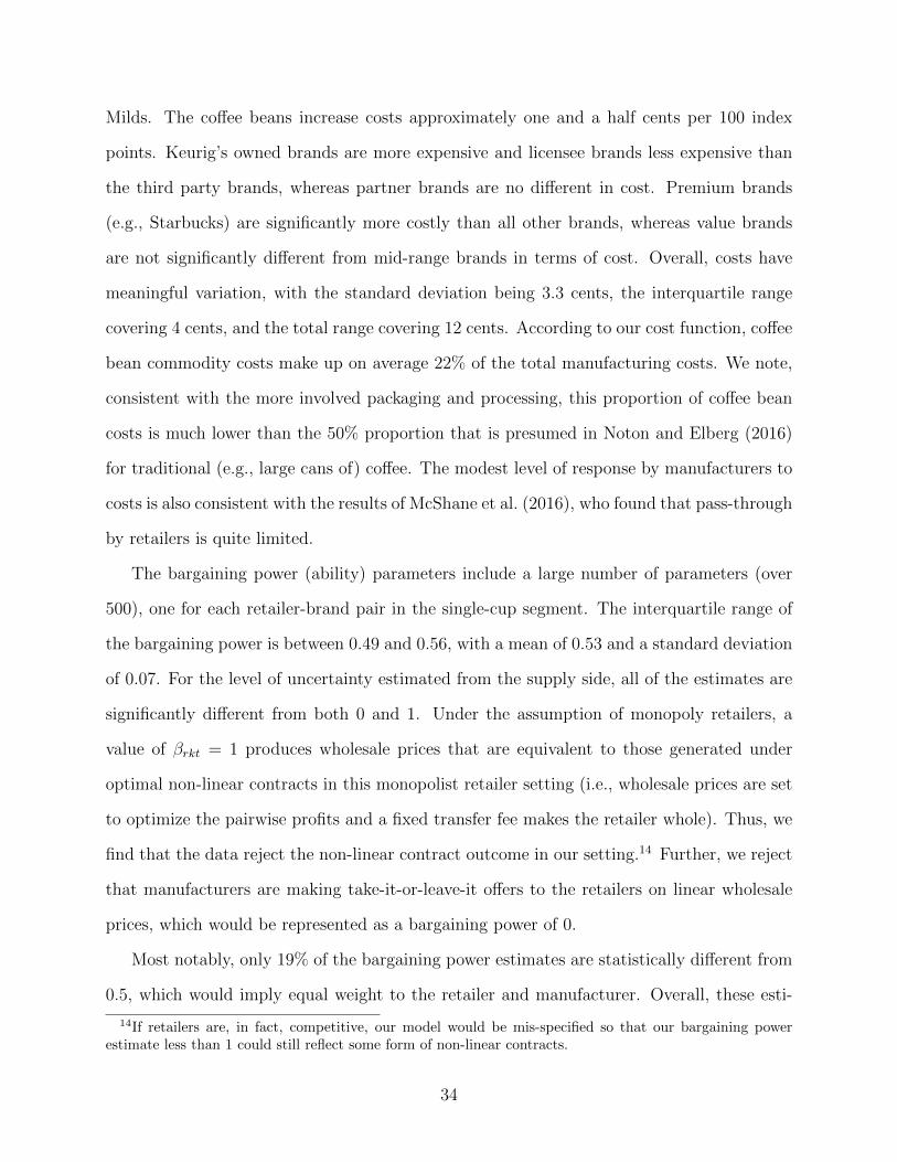
Milds. The coffee beans increase costs approximately one and a half cents per 100 index
points. Keurig’s owned brands are more expensive and licensee brands less expensive than
the third party brands, whereas partner brands are no different in cost. Premium brands
(e.g., Starbucks) are significantly more costly than all other brands, whereas value brands
are not significantly different from mid-range brands in terms of cost. Overall, costs have
meaningful variation, with the standard deviation being 3.3 cents, the interquartile range
covering 4 cents, and the total range covering 12 cents. According to our cost function, coffee
bean commodity costs make up on average 22% of the total manufacturing costs. We note,
consistent with the more involved packaging and processing, this proportion of coffee bean
costs is much lower than the 50% proportion that is presumed in Noton and Elberg (2016)
for traditional (e.g., large cans of) coffee. The modest level of response by manufacturers to
costs is also consistent with the results of McShane et al. (2016), who found that pass-through
by retailers is quite limited.
The bargaining power (ability) parameters include a large number of parameters (over
500), one for each retailer-brand pair in the single-cup segment. The interquartile range of
the bargaining power is between 0.49 and 0.56, with a mean of 0.53 and a standard deviation
of 0.07. For the level of uncertainty estimated from the supply side, all of the estimates are
significantly different from both 0 and 1. Under the assumption of monopoly retailers, a
value of βrkt = 1 produces wholesale prices that are equivalent to those generated under
optimal non-linear contracts in this monopolist retailer setting (i.e., wholesale prices are set
to optimize the pairwise profits and a fixed transfer fee makes the retailer whole). Thus, we
find that the data reject the non-linear contract outcome in our setting.14 Further, we reject
that manufacturers are making take-it-or-leave-it offers to the retailers on linear wholesale
prices, which would be represented as a bargaining power of 0.
Most notably, only 19% of the bargaining power estimates are statistically different from
0.5, which would imply equal weight to the retailer and manufacturer. Overall, these esti-
14If retailers are, in fact, competitive, our model would be mis-specified so that our bargaining powerestimate less than 1 could still reflect some form of non-linear contracts.
34

mates suggest a large degree of homogeneity across both retailers and brands in how much
bargaining power their behavior reflects. Further, the retailer and the brands appear to
have similar levels of bargaining power, consistent with the original symmetric formulation
proposed by Nash (1950). This seems quite reasonable in our context, as the asymmetric
bargaining power itself is intended to reflect differences in patience, tolerance for risk and
the negotiating skills of each party. It is hard to see why these should vary across the two
sides in this setting, given that, in most cases, both parties are large, often publicly traded
corporations with extensive experience in this market. In this case, large variation in the
estimated bargaining parameters might suggest that our measures of bargaining leverage
were incomplete, and there were other sizable determinants of the bargaining outcomes left
unaccounted for. This does not appear to be the case here.
We also examine whether the bargaining power parameters change after patent expi-
ration. We estimate models where we allow the average βrkt to differ the year before the
quarter of the patent expiration (quarter 12 when most private label entry occurs) and the
year after. The mean difference for a model with common changes for all RMAs is -0.0025
(t-stat=-0.41). Further, allowing RMA-level differences in the change in bargaining power
reveals only an average change of -0.004 and only 9 RMAs having more than a 0.02 shift.
Even at 0.02 the change in percent profit increase is quite small.15. Thus, our findings sug-
gest that most of the variation in outcomes with versus without the private label is due to
changes in the bargaining leverage of the two parties rather than bargaining power (ability).
This bargaining leverage is determined by the nature of demand and the brand equities (in-
tercepts) for the products each retailer carries. In particular, for our investigation into the
influence of private brand entry on bargaining outcomes, the private brand equity should be
a central determinant. As noted in section 4.1, we find considerable variation in these brand
intercepts across RMAs.
15The absolute change in percentage profit increase from adding the private label for a shift in bargainingpower of -0.004 is 0.07% and the larger shift of 0.02 is -0.3%. These are very small changes compared towhat is observed as the direct change in profit from adding the private label.
35
5 Counterfactual Experiments
In this section, we use counterfactual simulations to isolate and explore the impact of private
label entry on bargaining outcomes. Recall that much was changing in the single-cup market
over this period. The market for K-Cup coffee was continuing to expand with machine
ownership, branded firms that were unaffiliated with Keurig were entering the market (post
patent expiration), while new affiliated brands were entering in both periods, and most
retailers were launching new private label products (just after patent expiration). To control
for these factors and focus directly on the impact of private label entry, we consider a period
immediately after patent expiration and construct counterfactual outcomes for scenarios
both with and without private label products.
In particular, for each RMA where a private label was actually introduced, we simulate
a counterfactual outcome in which the private label product is removed from the market.
We compute the equilibrium (bargained) wholesale prices, the corresponding optimal retail
prices, and the resulting market shares. These counterfactual values will be denoted with a
superscript CF . We then compare these to the “factual” bargained wholesale prices, optimal
retailer prices and equilibrium market shares, computed with the private label in the market
and denoted with a superscript F . Note that both constructs are simulations, with the
latter corresponding to the “treatment” that actually occurred (i.e. private label entry) and
the former corresponding to the counterfactual “control” condition. We present measures
that reflect both the impact of the private label presence and the proportion that is due to
bargaining benefits versus category expansion. We use percentage changes throughout to
maintain a common scale. In all cases, we consider a setting in which all retailers choose
to have their store brand manufactured by a third-party supplier, as this corresponds to a
case in which retailers have the strongest bargaining leverage. For the following analyses,
we consider all 65 RMAs having 338 RMA-period cases with a (factual) private label entry
as compared to a (counterfactual) market without the private label.
36
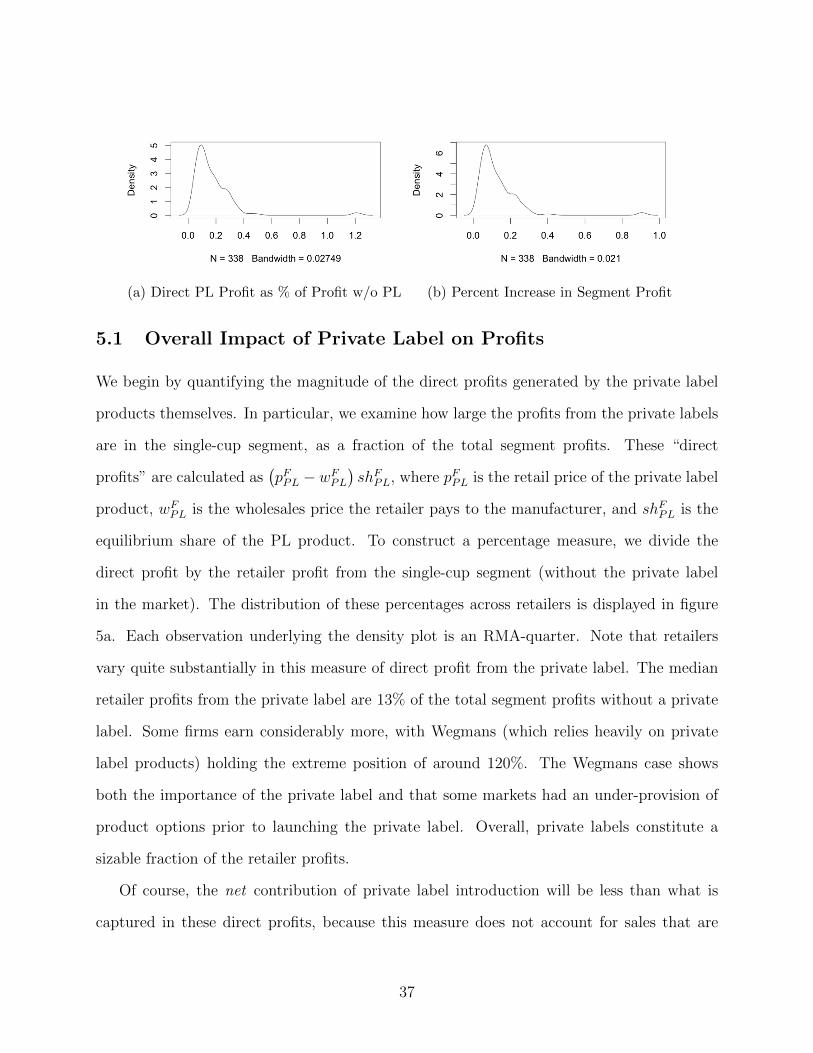
(a) Direct PL Profit as % of Profit w/o PL (b) Percent Increase in Segment Profit
5.1 Overall Impact of Private Label on Profits
We begin by quantifying the magnitude of the direct profits generated by the private label
products themselves. In particular, we examine how large the profits from the private labels
are in the single-cup segment, as a fraction of the total segment profits. These “direct
profits” are calculated as(pFPL − wFPL
)shFPL, where pFPL is the retail price of the private label
product, wFPL is the wholesales price the retailer pays to the manufacturer, and shFPL is the
equilibrium share of the PL product. To construct a percentage measure, we divide the
direct profit by the retailer profit from the single-cup segment (without the private label
in the market). The distribution of these percentages across retailers is displayed in figure
5a. Each observation underlying the density plot is an RMA-quarter. Note that retailers
vary quite substantially in this measure of direct profit from the private label. The median
retailer profits from the private label are 13% of the total segment profits without a private
label. Some firms earn considerably more, with Wegmans (which relies heavily on private
label products) holding the extreme position of around 120%. The Wegmans case shows
both the importance of the private label and that some markets had an under-provision of
product options prior to launching the private label. Overall, private labels constitute a
sizable fraction of the retailer profits.
Of course, the net contribution of private label introduction will be less than what is
captured in these direct profits, because this measure does not account for sales that are
37

diverted from the retailer’s other products. The net profit gain from introducing the private
label is presented in figure 5b, which shows the size of the percentage increase in overall
single-cup segment profits attributable to the introduction of a private label product. This
is calculated as the total retailer profit with the private label minus total retailer profit
without the private label divided by the total retailer profit without the private label. Note
that this calculation uses the same periods (i.e., not a before-after analysis). The lift is now
meaningfully smaller, though still quite large in magnitude. The median lift in overall profits
is 9.7%, with the extreme case of Wegmans at 93%. Private labels are a win for all retailers,
but some benefit substantially more than others.
5.2 Sources of Profit: Margin Improvement and Category Expan-
sion
We now consider how the profit gain is achieved. The private label can increase profit by
increasing the total category demand through the lower-priced product offering that draws
consumers away from the outside good and also can command a higher percentage margin.
Alternatively, the profit gain could come from increasing the margins of the existing products
without harming their sales too much.
Turning first to the total category expansion, we calculate the percentage increase in
singe-cup sales (out of total market size) with the private label versus without it. Figure 6a
indicates that the category expansion effect is quite large, increasing demand by an average
of 15%. This suggests there was pent-up demand for lower priced single-cup products and
that the private label satisfies a large segment of this unmet demand. Further, we also find
that (even) with the private label in the market, the average margin for the private labels
(52%) is higher than that of the leading national brand (47%). Note, however, that because
the category expansion arises largely due to the lower priced private label product, it is quite
possible that the average cents margin on product sold might actually fall.
We next examine how the margins on the national brands differ with versus without
38

(a) Percent Increase in Category DemandDue to PL
(b) Percent Increase in Margin on NationalBrands
the private label. In particular, we consider the margins the retailers are able to negotiate
with the national brands following the introduction of the private label product. Figure 6b
presents the density for the margin increase (on national brands) when the private label
is in the market versus the counterfactual outcome when the private label is absent. We
report this as a percentage of the counterfactual margin without the private label. While
the increase is relatively modest on average (2%) and most retailers see an increase of under
3%, again there is substantial heterogeneity, with some retailers achieving gains of 5% or
higher, some substantially less. This margin increase is part of the indirect benefit of private
label entry on the negotiations for the non-private label products.
5.3 Profit Decomposition and the Bargaining Benefit
We now evaluate the amount of profits arising from the bargaining benefit related to the
margin gain and category expansion. We first consider the category expansion. Category
expansion is the combination of an increase in shares due to the private label entering
(presumably at a lower price than the national brands) and a loss of shares (stolen) from
the national brands. Profits from category expansion are defined as
ΠCE =(pFPL − wFPL
)sFPL +
∑Jrt 6=PL
((pFj − wFj
) (sFj − sCFj
)(13)
39
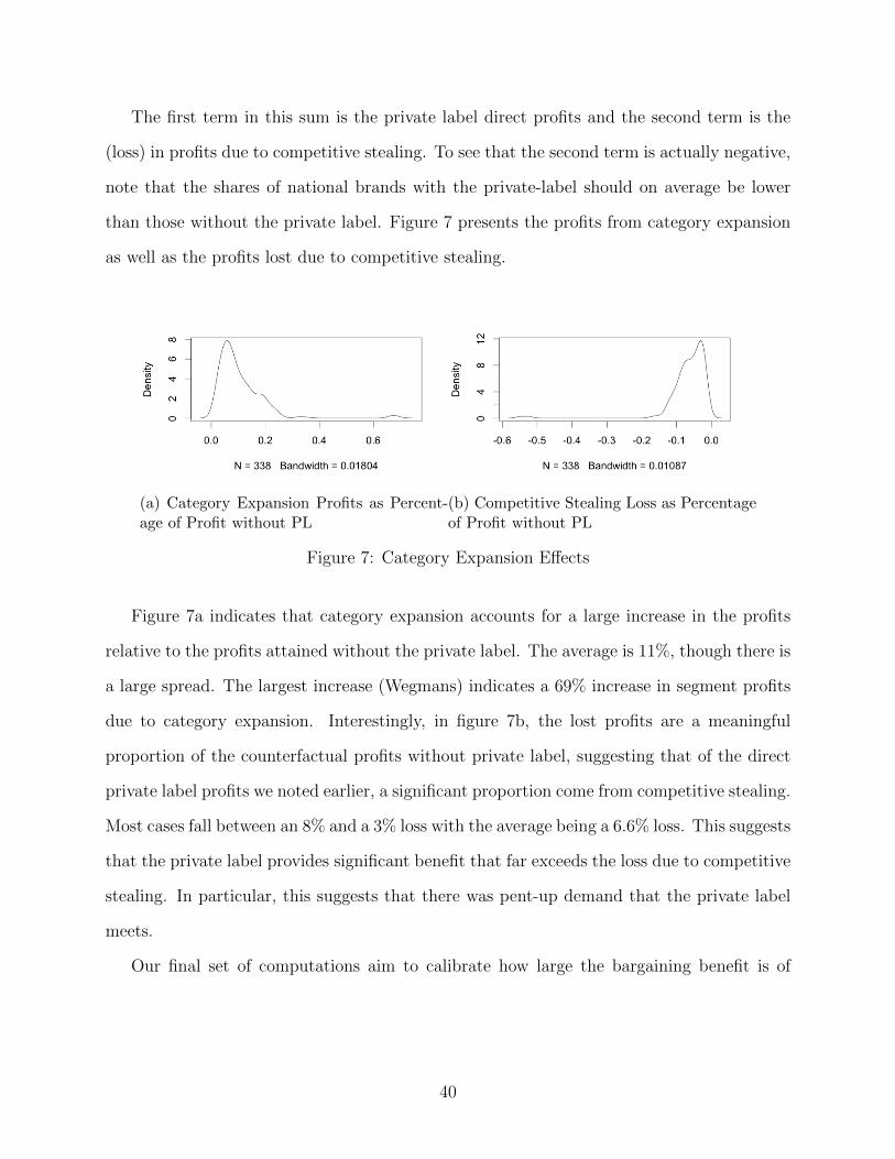
The first term in this sum is the private label direct profits and the second term is the
(loss) in profits due to competitive stealing. To see that the second term is actually negative,
note that the shares of national brands with the private-label should on average be lower
than those without the private label. Figure 7 presents the profits from category expansion
as well as the profits lost due to competitive stealing.
(a) Category Expansion Profits as Percent-age of Profit without PL
(b) Competitive Stealing Loss as Percentageof Profit without PL
Figure 7: Category Expansion Effects
Figure 7a indicates that category expansion accounts for a large increase in the profits
relative to the profits attained without the private label. The average is 11%, though there is
a large spread. The largest increase (Wegmans) indicates a 69% increase in segment profits
due to category expansion. Interestingly, in figure 7b, the lost profits are a meaningful
proportion of the counterfactual profits without private label, suggesting that of the direct
private label profits we noted earlier, a significant proportion come from competitive stealing.
Most cases fall between an 8% and a 3% loss with the average being a 6.6% loss. This suggests
that the private label provides significant benefit that far exceeds the loss due to competitive
stealing. In particular, this suggests that there was pent-up demand that the private label
meets.
Our final set of computations aim to calibrate how large the bargaining benefit is of
40
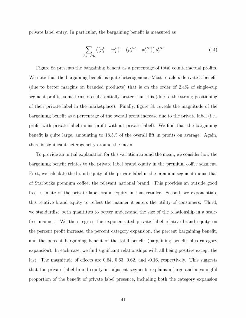
private label entry. In particular, the bargaining benefit is measured as
∑Jrt−PL
((pFj − wFj
)−(pCFj − wCFj
))sCFj (14)
Figure 8a presents the bargaining benefit as a percentage of total counterfactual profits.
We note that the bargaining benefit is quite heterogenous. Most retailers derivate a benefit
(due to better margins on branded products) that is on the order of 2.4% of single-cup
segment profits, some firms do substantially better than this (due to the strong positioning
of their private label in the marketplace). Finally, figure 8b reveals the magnitude of the
bargaining benefit as a percentage of the overall profit increase due to the private label (i.e.,
profit with private label minus profit without private label). We find that the bargaining
benefit is quite large, amounting to 18.5% of the overall lift in profits on average. Again,
there is significant heterogeneity around the mean.
To provide an initial explanation for this variation around the mean, we consider how the
bargaining benefit relates to the private label brand equity in the premium coffee segment.
First, we calculate the brand equity of the private label in the premium segment minus that
of Starbucks premium coffee, the relevant national brand. This provides an outside good
free estimate of the private label brand equity in that retailer. Second, we exponentiate
this relative brand equity to reflect the manner it enters the utility of consumers. Third,
we standardize both quantities to better understand the size of the relationship in a scale-
free manner. We then regress the exponentiated private label relative brand equity on
the percent profit increase, the percent category expansion, the percent bargaining benefit,
and the percent bargaining benefit of the total benefit (bargaining benefit plus category
expansion). In each case, we find significant relationships with all being positive except the
last. The magnitude of effects are 0.64, 0.63, 0.62, and -0.16, respectively. This suggests
that the private label brand equity in adjacent segments explains a large and meaningful
proportion of the benefit of private label presence, including both the category expansion
41

and bargaining benefits. Interestingly, the proportion of the total profit increase that is due
to the bargaining benefit decreases as brand equity increases. Although this relationship is
relatively weak, this relationship suggests that the retailers with the best private branding
programs tend to both expand the category and reap greater returns from national brands,
but grow the business (slightly) more than squeezing their suppliers.
(a) As Percentage of Profit without PL (b) As Percentage of Profit Increase
Figure 8: Bargaining Benefits
Counterfactual Outcome Estimate (Std. Err.) R2
% Profit Increase 0.638* (0.042) 0.407% Category Expansion 0.634* (0.042) 0.402%Bargain Benefit 0.621* (0.043) 0.386% of Profit Increase from Bargaining -0.157* (0.054) 0.025
Table 8: Regressions of Standardized Relative Brand Equity on Counterfactual Outcomes- *: p-value<.01
6 Conclusion
We examine the role of private labels in determining bargaining outcomes in the brew-at-
home coffee category. We exploit a natural experiment in which private label entry was
prevented by patent protection, to reveal how firms behave in the absence of private label
competition and how their strategies adapt when entry occurs. We find that bargaining
42

outcomes are driven primarily by bargaining leverage, while bargaining ability is relatively
symmetric. Moreover, the impact of bargaining leverage is substantial: bargaining benefits
account for roughly 20% of the overall benefit of private label introduction, which is itself
on the order of 10% of pre-introduction profits.
Note that we have abstracted away from competition between rival retailers. Extending
the analysis to include these effects is the subject of future research. Future work could
also consider how lump-sum transfers (e.g. slotting allowances and other non-linear con-
tracts) such as those considered in the theory work by Shaffer (2001) or alternative vertical
arrangements (e.g. non-cooperative vertical games) would change the analysis.
43

References
Berry, S., J. Levinsohn, and A. Pakes (1995). Automobile prices in market equilibrium.Econometrica 63 (4), 841–890.
Berry, S. T. and P. A. Haile (2014). Identification in differentiated products markets usingmarket level data. Econometrica 82 (5), 1749–1797.
Bonnet, C. and P. Dubois (2010). Inference on vertical contracts between manufacturersand retailers allowing for nonlinear pricing and resale price maintenance. RAND Journalof Economics 41 (1), 139–164.
Bresnahan, T. F. (1987). Competition and collusion in the american automobile industry:The 1955 price war. The Journal of Industrial Economics 35 (4), 457–482.
Bresnahan, T. F., S. Stern, and M. Trajtenberg (1997). Market segmentation and thesources of rents from innovation: Personal computers in the late 1980s. RAND Journal ofEconomics 28 (0), S17–S44.
Bronnenberg, B. J., J.-P. H. Dube, and M. Gentzkow (2012). The evolution of brand pref-erences: Evidence from consumer migration. American Economic Review 102 (6), 2472–2508.
Bruno, H. A. and N. J. Vilcassim (2008). Structural demand estimation with varying productavailability. Marketing Science 27 (6), 1126–1131.
Chintagunta, P. K., A. Bonfrer, and I. Song (2002). Investigating the effects of store-brandintroduction on retailer demand and pricing behavior. Management Science 48 (10), 1242–1267.
Collard-Wexler, A., G. Gowrisankaran, and R. S. Lee (2014). ‘Nash in Nash’ bargaining: Amicrofoundation for applied work. NBER Working Paper w20641.
Crawford, G. S., R. S. Lee, M. D. Whinston, and A. Yurukoglu (2015). The welfare effectsof vertical integration in multichannel television markets. NBER Working Paper.
Crawford, G. S. and A. Yurukoglu (2012). The welfare effects of bundling in multichanneltelevision markets. American Economic Review 102 (2), 643–685.
Dhar, S. K. and S. J. Hoch (1997). Why store brand penetration varies by retailer. MarketingScience 16 (3), 208–227.
Draganska, M., D. Klapper, and S. B. Villas-Boas (2010). A larger slice or a larger pie?An empirical investigation of bargaining power in the distribution channel. MarketingScience 29 (1), 57–74.
Gandhi, A. and J. Houde (2015). Measuring substitution patterns in differentiated productsindustries: The missing instruments. Working Paper (University of Pennsylvania).
44

Goldfarb, A., Q. Lu, and S. Moorthy (2009). Measuring brand value in an equilibriumframework. Marketing Science 28 (1), 69–86.
Gowrisankaran, G., A. Nevo, and R. Town (2014). Mergers when prices are negotiated:Evidence from the hospital industry. American Economic Review 105 (1), 172–203.
Grennan, M. (2013). Price discrimination and bargaining: Empirical evidence from medicaldevices. American Economic Review 103 (1), 145–177.
Hansen, K., V. Singh, and P. Chintagunta (2006). Understanding store-brand purchasebehavior across categories. Marketing Science 25 (1), 75–90.
Ho, K. (2009). Insurer-provider networks in the medical care market. American EconomicReview 99 (1), 393–430.
Ho, K. and R. S. Lee (2013). Insurer competition in health care markets. NBER WorkingPaper.
Hoch, S. J. and S. Banerji (1993). When do private labels succeed? Sloan managementreview 34 (4), 57–67.
Horn, H. and A. Wolinsky (1988). Bilateral monopolies and incentives for merger. RANDJournal of Economics 19 (3), 408–419.
Iyer, G. and J. M. Villas-Boas (2003). A bargaining theory of distribution channels. Journalof Marketing Research 40 (1), 80–100.
Judd, K. L. (1998). Numerical methods in economics. Cambridge, MA: MIT press.
McShane, B. B., C. Chen, E. T. Anderson, and D. I. Simester (2016). Decision stages andasymmetries in regular retail price pass-through. Marketing Science, Forthcoming.
Meza, S. and K. Sudhir (2010). Do private labels increase retailer bargaining power? Quan-titative Marketing and Economics 8 (3), 333–363.
Misra, S. and S. K. Mohanty (2006). Estimating bargaining games in distribution channels.Working Paper (University of Rochester).
Nash, J. F. (1950). The bargaining problem. Econometrica 18 (2), 155–162.
Nevo, A. (2000a). Mergers with differentiated products: The case of the ready-to-eat cerealindustry. RAND Journal of Economics 31 (3), 395–421.
Nevo, A. (2000b). A practitioner’s guide to estimation of random-coefficients logit modelsof demand. Journal of Economics & Management Strategy 9 (4), 513–548.
Nevo, A. (2001). Measuring market power in the ready-to-eat cereal industry. Economet-rica 69 (2), 307–342.
Nielsen Global Survey (2012). The State of private label around the world. The NielsenCompany.
45

Nijs, V., K. Misra, E. T. Anderson, K. Hansen, and L. Krishnamurthi (2010). Channelpass-through of trade promotions. Marketing Science 29 (2), 250–267.
Nijs, V. R., K. Misra, and K. Hansen (2013). Outsourcing retail pricing to a category captain:The role of information firewalls. Marketing Science 33 (1), 66–81.
Noton, C. and A. Elberg (2016). Are supermarkets squeezing small suppliers? Evidencefrom negotiated wholesale prices. Working Paper (University of Chile).
O’Brien, D. P. and G. Shaffer (2005). Bargaining, bundling, and clout: The portfolio effectsof horizontal mergers. RAND Journal of Economics 36 (3), 573–595.
Pauwels, K. and S. Srinivasan (2004). Who benefits from store brand entry? MarketingScience 23 (3), 364–390.
Rubinstein, A. (1982). Perfect equilibrium in a bargaining model. Econometrica 50 (1),97–109.
Sayman, S., S. J. Hoch, and J. S. Raju (2002). Positioning of store brands. MarketingScience 21 (4), 378–397.
Schultz, H. (2012). Private labels sales hit $98 billion on 6% growth, report says. FoodNavigator USA.
Scott Morton, F. and F. Zettelmeyer (2004). The strategic positioning of store brands inretailer–manufacturer negotiations. Review of Industrial Organization 24 (2), 161–194.
Shaffer, G. (2001). Bargaining in distribution channels with multiproduct retailers. Technicalreport, mimeo, University of Rochester.
Tenn, S. and J. M. Yun (2008). Biases in demand analysis due to variation in retail distri-bution. International Journal of Industrial Organization 26 (4), 984–997.
Villas-Boas, S. B. (2007). Vertical relationships between manufacturers and retailers: Infer-ence with limited data. Review of Economic Studies 74 (2), 625–652.
Werden, G. J. and L. M. Froeb (1994). The effects of mergers in differentiated productsindustries: Logit demand and merger policy. Journal of Law, Economics, & Organiza-tion 10 (2), 407–426.
46

A Details of Sample Construction
In this appendix, we discuss details of the sample selection and segment definitions used inour empirical analyses.
We begin by discussing details about how we categorize the product segments. Thepremium segment includes all whole bean coffee products and ground coffee brands thatmainly sold in premium packages such as bag or foil pouch. We then categorize the groundcoffee brands that are mainly sold in can or canister and are cheap (i.e., below $0.15 perserving to be defined below) as the mainstream segment. For products in other package typessuch as brick and box, we categorize them into the premium segment if their price per poundis in the range of the whole bean and bagged ground coffee, or the mainstream otherwise.For the instant segment, we use the IRI subcategory definition to identify instant, namely,soluble coffee products. Finally, for the single cup segment, we follow the IRI subcategorydefinition to identify single cup products. Furthermore, for the purpose of our study, weexclude single cup coffee products that are not compatible with the Keurig K-Cup system,which we identify through product formats (for example, T Disc and Vue are not compatiblewith the Keurig K-Cup brewer). Note that in 2008, Keurig K-Cup compatible products were87% of the whole single cup segment in revenue. This portion increases in subsequent years,reaching 99% in 2014.
In order to construct prices that are comparable across segments, we define the equivalentserving size for each segment, namely, the weight of coffee products to make a standard cupof coffee (6 fluid oz.). For the mainstream and premium products, we apply a universalserving size 0.4 oz. per cup of coffee. For mix or flavored instant products, we follow themanufacturer’s recommendation for each brand to define the equivalent serving size; forregular instant product, we apply a universal serving size 2/15 oz. For single cup products,one pod is equivalent to one serving.
For each segment, we keep the leading national brands based on their total dollar salesin the sample. Table A.1 reports all the brands we include in our sample. Note that we keepmore brands in the single cup segment than other segments, since that is the focal segmentof this study. For each RMA, we drop segment-brands that only appear once in the entiresample period to avoid singularities when estimating demand. These single period cases arerare and unusual. The remaining sample captures 93.7% of total coffee sales. Finally, weselect the RMA-week-segment-brand observations that have a reasonable level of distributionto better capture representative patterns of demand. First, we drop observations with lessthan 10% ACV distribution. We found these observations to be more likely to be error-prone and they had little impact on the total sales. Second, we drop any segment-brand inan RMA if its median ACV distribution fails to ever achieve 50% (medians are calculatedafter the censoring). These segment-brands represent relatively small share cases and, withthis selection criteria, we retain 87.1% of the remaining observations and 98.3% of remainingdollar sales.
We also note that we group the Keurig owned K-Cup brands, including Keurig’s leadinghouse brand Green Mountain and other smaller brands. The full list of grouped brands areBARISTA PRIMA, CAFE ESCAPES, COFFEE PEOPLE, DIEDRICH, DONUT HOUSECOLLECTION, DONUT SHOP, GREEN MOUNTAIN, KEURIG EMERILS, KEURIGGLORIA JEANS, KEURIG KAHLUA COFFEE, KEURIG MIX VARIETY, KEURIG TIM-
47

OTHY’S, KEURIG WOLFGANG PUCK, REVV, TULLYS COFFEE, and VAN HOUTTE.In general, these brands’ prices and price promotion schedules are closely linked, lending sup-port to the aggregation we do. We studied a sample of fourteen RMAs in detail to evaluatewhether the pricing of these brands were indeed closely linked. We considered the brandsthat make up 95% of the Keurig Owned brand sales and that were in the sample at least52 weeks. These brands were Cafe Escapes (2.5%), Donut House (17.2%), Green Mountain(62.7%), and Tully’s (12.7%). First, the bulk of the owned sales is actually from the singleGreen Mountain brand with the rest relatively spread out. Second, we found that thesefour brands have TPR promotion schedules that are closely linked with their average priceshaving sharp dips at the same time and prices are correlated within RMA. For example, theaverage correlation between Donut House and Green Mountain is 0.68 and between Tully’sand Green Mountain is 0.78. Third, the weekly prices of these brands within an RMA haveprices within 1 cent 46% of the time, within 5 cents 66% of the time and within 10 cents82% of the time on average across the RMAs.
The above describes the sample construction for the demand-side estimation. The supply-side has several additional considerations. First, we aggregate our data to the quarterly level(13 week periods). To do so, we construct a measure of regular prices as the 90th quantile ofthe weekly price distribution in the quarter and construct averages for the other quantities ofinterest (e.g., ACV, share). Second, in the supply side estimation, we include only the single-cup products in the bargaining set and don’t consider the main, premium, or instant coffeeproducts. This simplification reduces the computational burden of the problem, focuses onour main interest, and is justifiable because the substitution between single-cup and theother segments is relatively small. Third, we consider only the period from 2010 onward(ending after the first quarter of 2014) to use data more proximate in time to the privatelabel entries for estimating the cost function.
Fourth, we use the sample selection rules discussed above and add some additional onesresulting from some measurement concerns due to aggregating to the quarter. We include inthe profit calculations only brands that are observed at least 6 of the 13 weeks and includeas bargaining observations to calculate the moments only those brands that have at least10 weeks of data in the given quarter. This largely eliminates cases when a brand firstenters the market or just before it exits. These cases often have lower ACV, have unusualpromotional activity, and our measures for the quarter tend to be poor approximations torapidly changing shares. In addition to this rule, we identified three other observationswhere our quarterly measures appeared to have substantial error, and dropped those casesas well. After all of these additional sample adjustments, we retain 6,978 observations or92% of the original bargaining observations (i.e., quarter RMA-brand-retailer pairs). Thesebargaining observations are spread across the 72 RMAs and 17 quarters. We note that mostof the bargaining pair observations have 3 or more brands in the market (86%) and 10 orless (88%).
B Installed Base Imputation
We use the single cup category penetration rate (percent households ever purchased in ayear) as a proxy for the installed base of Keurig brewers among retailer shoppers. The
48
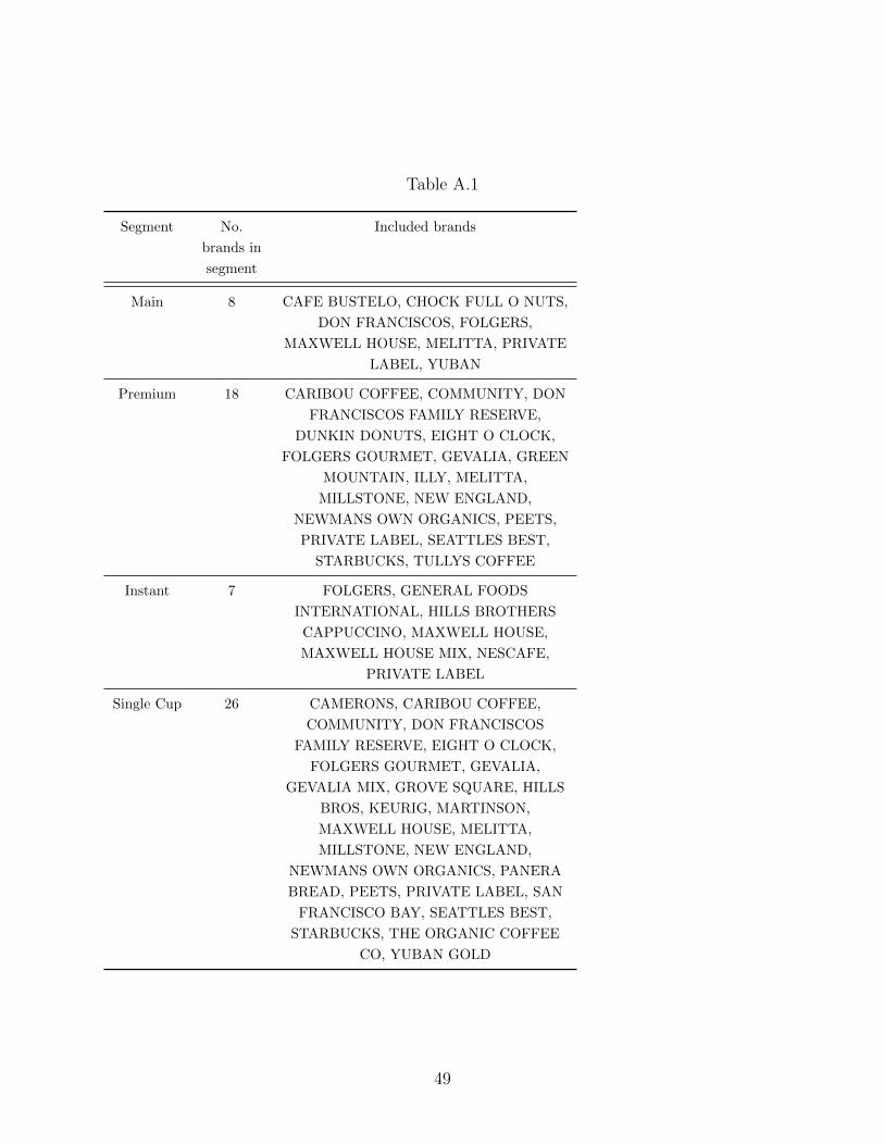
Table A.1
Segment No.
brands in
segment
Included brands
Main 8 CAFE BUSTELO, CHOCK FULL O NUTS,
DON FRANCISCOS, FOLGERS,
MAXWELL HOUSE, MELITTA, PRIVATE
LABEL, YUBAN
Premium 18 CARIBOU COFFEE, COMMUNITY, DON
FRANCISCOS FAMILY RESERVE,
DUNKIN DONUTS, EIGHT O CLOCK,
FOLGERS GOURMET, GEVALIA, GREEN
MOUNTAIN, ILLY, MELITTA,
MILLSTONE, NEW ENGLAND,
NEWMANS OWN ORGANICS, PEETS,
PRIVATE LABEL, SEATTLES BEST,
STARBUCKS, TULLYS COFFEE
Instant 7 FOLGERS, GENERAL FOODS
INTERNATIONAL, HILLS BROTHERS
CAPPUCCINO, MAXWELL HOUSE,
MAXWELL HOUSE MIX, NESCAFE,
PRIVATE LABEL
Single Cup 26 CAMERONS, CARIBOU COFFEE,
COMMUNITY, DON FRANCISCOS
FAMILY RESERVE, EIGHT O CLOCK,
FOLGERS GOURMET, GEVALIA,
GEVALIA MIX, GROVE SQUARE, HILLS
BROS, KEURIG, MARTINSON,
MAXWELL HOUSE, MELITTA,
MILLSTONE, NEW ENGLAND,
NEWMANS OWN ORGANICS, PANERA
BREAD, PEETS, PRIVATE LABEL, SAN
FRANCISCO BAY, SEATTLES BEST,
STARBUCKS, THE ORGANIC COFFEE
CO, YUBAN GOLD
49
point-of-sale data starts from 2008 yet the penetration rate data are only available startingfrom 2011.16 In order to obtain installed base prior to 2011, we fit a bass diffusion curvefor each individual RMA with the initial year being 2004 when the first Keurig at-homesingle cup brewer was introduced. The bass diffusion process is described by the followingequation. We estimate the bass diffusion parameters for each RMA using nonlinear leastsquares.
IBjt = mj ∗1− exp (−(pj + qj) ∗ (t− t0))
1 +qjpj
exp (−(pj + qj) ∗ (t− t0))(15)
where j represents retailers, t represents year, and t0 = 2004. We then use the fitted value asthe end of year installed base throughout the sample (i.e., not only to make up for the missingpenetration rates but also the observed values) to smooth out noises from the penetrationrate data. In addition, recognizing that the penetration rate likely captures a subset of theactual Keurig owners among the retailer shoppers (namely, leaving out those who own aKeurig but never buy single cup from that retailer), we increase the fitted value by threepercentage points.17 Finally, we interpolate the end of year installed base to end of quarterones by assigning 13%, 14%, 25%, and 48% increment to each calendar quarter respectivelybased on Keurig’s quarterly national sales in their 2013 10Q report. Weekly installed baselevels are interpolated linearly from these quarterly levels.
C Keurig Brewer Prices
Figure C.1 presents brewer prices across retailers aggregated to the model level. The brewerprices seem largely unaffected by the patent expiration with only two potential exceptions.The first, the Keurig Elite model, appears to have a permanent price drop following thepatent expiration. This price drop is actually arising from a single retailer and not a sys-tematic effect. The other case is a Mr. Coffee model that experiences a temporary pricepromotion shortly after the patent expiration. However, this price drop appears to be con-sistent in size with later price promotions. Examination of the individual SKUs presentssimilar findings. Hence, brewer prices appear unlikely to influence the analysis and resultspresented in this paper.
D Corner cases of the bargaining model
The bargaining power parameter in the Nash bargaining model indexes a range of potentialsupply arrangements. Two corner cases with β = 1 and β = 0 correspond to two special
16Some RMA-years had too few buyers in the IRI panel data to make a projection to the shopper populationfor that specific RMA-year of the percentage of shoppers that buy any single-cup products. We use thefitted values of a multiple regression to impute the missing values, where the regression includes independentvariables the (raw, not projected) observed number of buyers divided by the raw number of shoppers, theshare of the K-Cup sales out of coffee sales, total K-Cup and total coffee sales, average dollar sales weightedACV for K-Cup products, the average, minimum, and maximum number of K-Cup brands (and polynomialsof these), and a cubic function of the year dummies interacted with the coffee penetration rate.
17We determined the 3% value by analyzing the category share out of total coffee to infer a lower boundof the installed base.
50
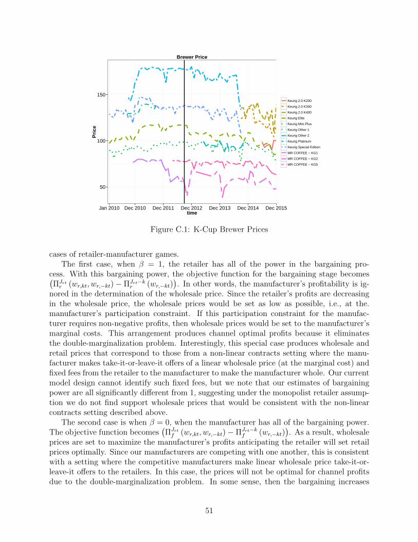
50
100
150
Jan 2010 Dec 2010 Dec 2011 Dec 2012 Dec 2013 Dec 2014 Dec 2015time
Pric
eKeurig 2.0 K200
Keurig 2.0 K300
Keurig 2.0 K400
Keurig Elite
Keurig Mini Plus
Keurig Other 1
Keurig Other 2
Keurig Platinum
Keurig Special Edition
MR COFFEE − KG1
MR COFFEE − KG2
MR COFFEE − KG5
Brewer Price
Figure C.1: K-Cup Brewer Prices
cases of retailer-manufacturer games.The first case, when β = 1, the retailer has all of the power in the bargaining pro-
cess. With this bargaining power, the objective function for the bargaining stage becomes(ΠJrtr (wr,kt, wr,−kt)− ΠJrt−k
r (wr,−kt)). In other words, the manufacturer’s profitability is ig-
nored in the determination of the wholesale price. Since the retailer’s profits are decreasingin the wholesale price, the wholesale prices would be set as low as possible, i.e., at the.manufacturer’s participation constraint. If this participation constraint for the manufac-turer requires non-negative profits, then wholesale prices would be set to the manufacturer’smarginal costs. This arrangement produces channel optimal profits because it eliminatesthe double-marginalization problem. Interestingly, this special case produces wholesale andretail prices that correspond to those from a non-linear contracts setting where the manu-facturer makes take-it-or-leave-it offers of a linear wholesale price (at the marginal cost) andfixed fees from the retailer to the manufacturer to make the manufacturer whole. Our currentmodel design cannot identify such fixed fees, but we note that our estimates of bargainingpower are all significantly different from 1, suggesting under the monopolist retailer assump-tion we do not find support wholesale prices that would be consistent with the non-linearcontracts setting described above.
The second case is when β = 0, when the manufacturer has all of the bargaining power.The objective function becomes
(ΠJrtf (wr,kt, wr,−kt)− ΠJrt−k
f (wr,−kt)). As a result, wholesale
prices are set to maximize the manufacturer’s profits anticipating the retailer will set retailprices optimally. Since our manufacturers are competing with one another, this is consistentwith a setting where the competitive manufacturers make linear wholesale price take-it-or-leave-it offers to the retailers. In this case, the prices will not be optimal for channel profitsdue to the double-marginalization problem. In some sense, then the bargaining increases
51

channel profits and also the share that the retailer obtains as the β increases.
E Additional Calculations
For simplicity, we drop the krt subscripts and letting wf and cf represent the vector ofwholesale prices and marginal costs for brands owned by manufacturer f . To accommodatethe partner revenue sharing we develop the notation µ1j and µ2j. We let µ1j to be 1 − κfor the profits for partner brands, κ for Keurig profits, and 1 otherwise. We let µ2j to be 0for Keurig profits and 1 otherwise. With this notation, the manufacturer profits in matrixnotation are ∑
j∈frt
(wjµ1j − cjµ2j) sJrtj (p) (16)
We denote the vector of µ1j containing all terms relevant for manufacturer f to be µf1and likewise for µf2 . The derivatives in terms of the wholesale price are then
dF
dwk=
∑j∈f
(wjµ1j − cjµ2j)dsjdwk
+ skµ1k (17)
=(wf · µf1 − cf · µ
f2
)′ dsdwk
+ skµ1k (18)
dR
dwk=
∑j∈J
((pj − wj)
dsjdwk
+dpjdwk
sj
)− sk (19)
= (p− w)′ds
dwk+
(dp
dwk
)′s− sk. (20)
(21)
We now consider the calculation of the two total derivatives contained in these ex-pressions,
dsjdwk
anddpjdwk
. For the former, note that sj = sj (p1 (wk) , . . . , pJ (wk)), so thatdsjdwk
=∑J
l=1∂sj∂pl
dpldwk
. In matrix notation, this is −Ω dpdwk
, where the lth row and jth column ofΩ is
−dsjdpl
=
if j = l −
∫i
sji(1−sji)αi
pjdθi
if j 6= l∫i
sjisliαi
pldθi
, (22)
where θi represents the set of all individual level variables characterizing heterogeneity, i.e.,including tastes, price sensitivity, availability, and machine ownership.
Combining the columns for the derivatives of F and R in terms of w and expressing thesederivatives more fully, we have
52
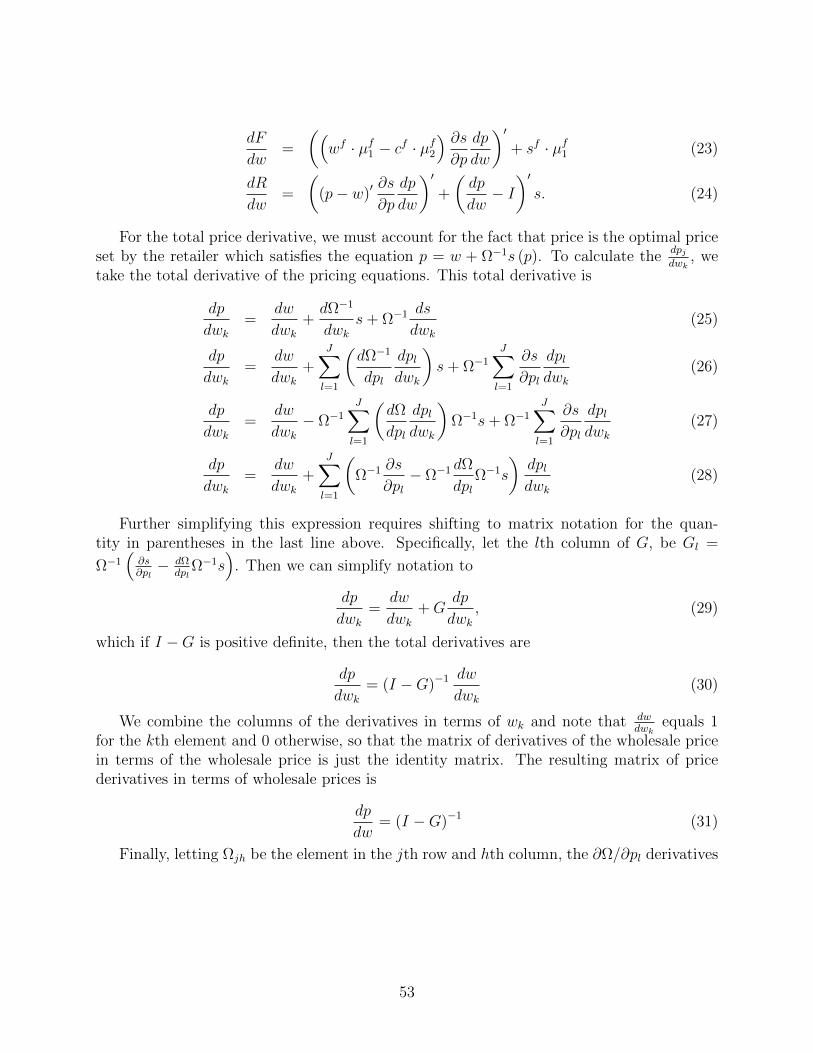
dF
dw=
((wf · µf1 − cf · µ
f2
) ∂s∂p
dp
dw
)′+ sf · µf1 (23)
dR
dw=
((p− w)′
∂s
∂p
dp
dw
)′+
(dp
dw− I)′s. (24)
For the total price derivative, we must account for the fact that price is the optimal priceset by the retailer which satisfies the equation p = w + Ω−1s (p). To calculate the
dpjdwk
, wetake the total derivative of the pricing equations. This total derivative is
dp
dwk=
dw
dwk+dΩ−1
dwks+ Ω−1 ds
dwk(25)
dp
dwk=
dw
dwk+
J∑l=1
(dΩ−1
dpl
dpldwk
)s+ Ω−1
J∑l=1
∂s
∂pl
dpldwk
(26)
dp
dwk=
dw
dwk− Ω−1
J∑l=1
(dΩ
dpl
dpldwk
)Ω−1s+ Ω−1
J∑l=1
∂s
∂pl
dpldwk
(27)
dp
dwk=
dw
dwk+
J∑l=1
(Ω−1 ∂s
∂pl− Ω−1 dΩ
dplΩ−1s
)dpldwk
(28)
Further simplifying this expression requires shifting to matrix notation for the quan-tity in parentheses in the last line above. Specifically, let the lth column of G, be Gl =
Ω−1(∂s∂pl− dΩ
dplΩ−1s
). Then we can simplify notation to
dp
dwk=
dw
dwk+G
dp
dwk, (29)
which if I −G is positive definite, then the total derivatives are
dp
dwk= (I −G)−1 dw
dwk(30)
We combine the columns of the derivatives in terms of wk and note that dwdwk
equals 1for the kth element and 0 otherwise, so that the matrix of derivatives of the wholesale pricein terms of the wholesale price is just the identity matrix. The resulting matrix of pricederivatives in terms of wholesale prices is
dp
dw= (I −G)−1 (31)
Finally, letting Ωjh be the element in the jth row and hth column, the ∂Ω/∂pl derivatives
53
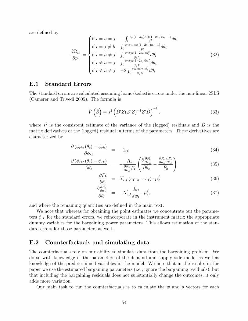
are defined by
∂Ωjh
∂pl=
if l = h = j −∫isli(1−sli)αi((1−2sli)αi−1)
p2l
dθi
if l = j 6= h∫islishiαi((1−2sli)αi−1)
p2l
dθi
if l = h 6= j∫i
slisji(1−2sli)α2i
pjpldθi
if l 6= h = j∫i
slisji(1−2sji)α2i
pjpldθi
if l 6= h 6= j −2∫i
sjislishiα2i
pjpldθi
(32)
E.1 Standard Errors
The standard errors are calculated assuming homoskedastic errors under the non-linear 2SLS(Camerer and Trivedi 2005). The formula is
V(β)
= s2(D′Z(Z ′Z)−1Z ′D
)−1
, (33)
where s2 is the consistent estimate of the variance of the (logged) residuals and D is thematrix derivatives of the (logged) residual in terms of the parameters. These derivatives arecharacterized by
∂ (φrkt (θc)− φrk)∂φrk
= −1rk (34)
∂ (φrkt (θc)− φrk)∂θc
= − Rk
∂Rk
∂wkFk
(∂ ∂Fk
∂wk
∂θc−
∂Fk
∂wk
∂Fk
∂θc
Fk
)(35)
∂Fk∂θc
= X′
c,f (sf−k − sf ) · µf2 (36)
∂ ∂Fk
∂wk
∂θc= −X ′
c,f
dsfdwk· µf2 , (37)
and where the remaining quantities are defined in the main text.We note that whereas for obtaining the point estimates we concentrate out the parame-
ters φrk for the standard errors, we reincorporate in the instrument matrix the appropriatedummy variables for the bargaining power parameters. This allows estimation of the stan-dard errors for those parameters as well.
E.2 Counterfactuals and simulating data
The counterfactuals rely on our ability to simulate data from the bargaining problem. Wedo so with knowledge of the parameters of the demand and supply side model as well asknowledge of the predetermined variables in the model. We note that in the results in thepaper we use the estimated bargaining parameters (i.e., ignore the bargaining residuals), butthat including the bargaining residuals does not substantially change the outcomes, it onlyadds more variation.
Our main task to run the counterfactuals is to calculate the w and p vectors for each
54

period and market. The optimal p vector can be calculated for any given w by successiveapproximation on the price first order conditions, p = w+Ω (p)−1 s (p). With the monopolistretailer assumptions, these conditions represent a unique equilibrium.
Our counterfactuals are calculated by proposing the set of products in the bargainingsetting and then guessing at the wholesale price, w, and solving for p. With these quantitiesin hand, we use the first order conditions of the bargaining problem to solve for the w viasuccessive approximation (we have also done this with non-linear solvers). The successiveapproximation takes the following form:
wh+1 = cµ2
µ1
−s(wh)
+ V(wh)
Ψ (wh) · µ1
, (38)
where h indexes the iterations, w, c, and s are the respective Jx1 vectors of wholesale prices,costs, and shares, V is a Jx1 vector that represents the internalization of the profit impactof this bargain on other products the manufacturer controls, and Ψ is Jx1 vector related toa ”mark-up” term. The jth element of Ψ is
Ψ(j) =dsjdwj
+ ρjsj, (39)
where ρj is defined by
ρj =βj
1− βj
dRj
dwj
Rj
, (40)
and the diagonal matrix with ρj on the (j, j)th element is ρ. V is defined by
V =
(M ∗ (1− I) ∗
(ds
dw+ ρs
))· (w · µ1 − c · µ2) , (41)
where s is a JxJ matrix with the (j, k) element containing the difference between the shareof product k with all products versus the share without product j, where the retail pricesare set optimally given the wholesale price and the set of products in the market. Thematrices M ∗ (1− I) are element-wise multiplied and represent the ownership structure withthe diagonal elements containing zeros.
The derivation of equation (38) relies on separating the jth (bargained) product fromdFj/dwj and Fj, moving that to the lefthand side and separating wj from the other terms.
We note that we have no proof that the bargaining problem has a unique equilibrium.We try multiple starting points in order to evaluate whether multiple equilibria are obtained.
55
Recommended