Probabilistic Backpropagation forScalable Learning of Bayesian Neural Networks
Jose Miguel Hernandez-Lobato
joint work with Ryan P. Adams
Workshop on Gaussian Process Approximations
May 21, 2015

Infinitely-big Bayesian Neural Networks
• Neal [1996] showed that a neural network (NN) converges to aGaussian Process (GP) as the number of hidden units increases.
• GPs allow for exact Bayesian inference. Learning infinitely-bigBayesian networks is then easier and more robust to overfitting.
−6 −4 −2 0 2 4
−50
050
Neural Network Predictions
x
y
−6 −4 −2 0 2 4
−50
050
Gaussian Process Predictions
x
y
1/17

Sparse Gaussian Processes
• The price paid is in scalability. From O(n) we go to O(n3). TheNon-parametric approach is infeasible with massive data!
• Solution: transform the full GP back into a sparse GPs using minducing points. From O(n3) we go back to O(n).
−6 −4 −2 0 2 4
−50
050
Full Gaussian Process Predictions
x
y
−6 −4 −2 0 2 4
−50
050
Sparse Gaussian Process Predictions
x
y − − − −− − − −
2/17
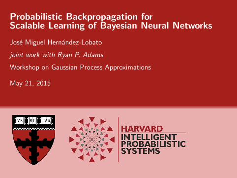
Sparse Gaussian Processes as Parametric Methods
FITC approximation: the most widely used method for sparse GPs.
The evaluations f of the function are conditionally independent giventhe value u of the function at the m inducing points:
p(f|u) ≈ p(f|u) =n∏
i=1
N (fi |Kfi ,uK−1uu u, kfi fi −KfiuK−1uu Kufi ) .
The values u at the inducing points are the parameters of the sparse GP.
A Gaussian approximation q(u) = N (u|m,V) can then be adjusted tothe posterior on u using scalable stochastic and distributed VI or EP(Hensman et al. [2013, 2014], Hernandez-Lobato et al. [2015]).
Is the cycle parametric → non-parametric → parametric worth it?Perhaps, because scalable inference in NNs is very hard, or perhaps not...
3/17
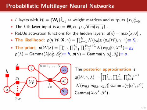
Probabilistic Multilayer Neural Networks
• L layers with W = {Wl}Ll=1 as weight matrices and outputs {zl}Ll=0.
• The l-th layer input is al = Wlzl−1/√
dim(zl−1) .
• ReLUs activation functions for the hidden layers: a(x) = max(x , 0) .
• The likelihood: p(y|W,X, γ) =∏N
n=1N (yn|zL(xn|W), γ−1)≡ fn .
• The priors: p(W|λ) =∏L
l=1
∏Vli=1
∏Vl−1+1j=1 N (wij ,l |0, λ−1)≡ gk ,
p(λ) = Gamma(λ|αλ0 , βλ0 )≡ h, p(γ) = Gamma(γ|αγ0 , βγ0 )≡ s .
The posterior approximation is
q(W, γ, λ) =[∏L
l=1
∏Vli=1
∏Vl−1+1j=1
N (wij ,l |mij ,l , vij ,l)] Gamma(γ|αγ , βγ)
Gamma(λ|αλ, βλ) .
4/17
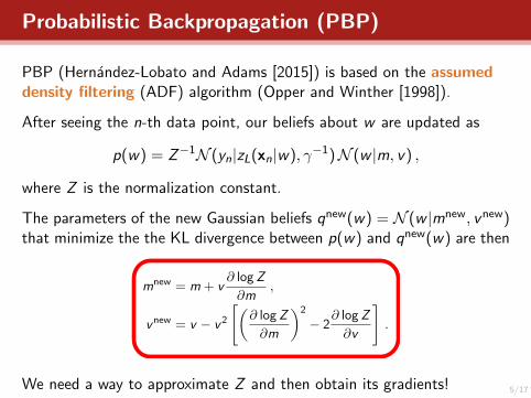
Probabilistic Backpropagation (PBP)
PBP (Hernandez-Lobato and Adams [2015]) is based on the assumeddensity filtering (ADF) algorithm (Opper and Winther [1998]).
After seeing the n-th data point, our beliefs about w are updated as
p(w) = Z−1N (yn|zL(xn|w), γ−1)N (w |m, v) ,
where Z is the normalization constant.
The parameters of the new Gaussian beliefs qnew(w) = N (w |mnew, vnew)that minimize the the KL divergence between p(w) and qnew(w) are then
We need a way to approximate Z and then obtain its gradients! 5/17

Forward Pass
Propagate distributions through the network and approximate themwith Gaussians by moment matching.
6/17

Backward Pass and Implementation Details
Once we compute log Z , we obtain its gradients by backpropagation.
Like in classic backpropagation, we obtain a recursion in terms of deltas:
δmj =∂ log Z
∂maj
=∑
k∈O(j)
{δmk∂ma
k
∂maj
+ δvk∂va
k
∂maj
},
δvj =∂ log Z
∂vaj
=∑
k∈O(j)
{δmk∂ma
k
∂vaj
+ δvk∂va
k
∂vaj
}.
Can be automatically implemented with Theano or autograd.
Implementation details:
• Approximation of the Student’s t likelihood with a Gaussian.
• We do several passes over the data with ADF.
• The approximate factors for the prior are updated using EP.
• Posterior approximation q initialized with random mean value.7/17

Results on Toy Dataset
40 training epochs.
100 hidden units.
VI uses two stochasticapproximations to the lowerbound (Graves [2011]).
BP and VI tuned withBayesian optimization(www.whetlab.com).
−6 −4 −2 0 2 4
−50
050
−6 −4 −2 0 2 4
−50
050
−6 −4 −2 0 2 4
−50
050
−6 −4 −2 0 2 4
−50
050
8/17

Exhaustive Evaluation on 10 Datasets
Table : Characteristics of the analyzed data sets.
Dataset N d
Boston Housing 506 13Concrete Compression Strength 1030 8Energy Efficiency 768 8Kin8nm 8192 8Naval Propulsion 11,934 16Combined Cycle Power Plant 9568 4Protein Structure 45,730 9Wine Quality Red 1599 11Yacht Hydrodynamics 308 6Year Prediction MSD 515,345 90
Always 50 hidden units except in Year and Protein where we use 100.
9/17

Average Test RMSE
Table : Average test RMSE and standard errors.
Dataset VI BP PBPBoston 4.320±0.2914 3.228±0.1951 3.010±0.1850Concrete 7.128±0.1230 5.977±0.2207 5.552±0.1022Energy 2.646±0.0813 1.185±0.1242 1.729±0.0464Kin8nm 0.099±0.0009 0.091±0.0015 0.096±0.0008Naval 0.005±0.0005 0.001±0.0001 0.006±0.0000Power Plant 4.327±0.0352 4.182±0.0402 4.116±0.0332Protein 4.842±0.0305 4.539±0.0288 4.731±0.0129Wine 0.646±0.0081 0.645±0.0098 0.635±0.0078Yacht 6.887±0.6749 1.182±0.1645 0.922±0.0514Year 9.034±NA 8.932±NA 8.881± NA
10/17
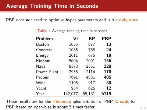
Average Training Time in Seconds
PBP does not need to optimize hyper-parameters and is run only once.
Table : Average running time in seconds.
Problem VI BP PBPBoston 1035 677 13Concrete 1085 758 24Energy 2011 675 19Kin8nm 5604 2001 156Naval 8373 2351 220Power Plant 2955 2114 178Protein 7691 4831 485Wine 1195 917 50Yacht 954 626 12Year 142,077 65,131 6119
These results are for the Theano implementation of PBP. C code forPBP based on open-blas is about 5 times faster. 11/17

Comparison with Sparse GPs
VI implementation described by Hensman et al. [2014].Same number m of pseudo-inputs as hidden units in neural networks.Stochastic optimization with ADADELTA and minibatch size m.
Table : Average Test Log-likelihood.
Dataset SGP PBPBoston -2.614±0.074 -2.577±0.095Concrete -3.417±0.031 -3.144±0.022Energy -1.612±0.022 -1.998±0.020Kin8nm 0.872±0.008 0.919±0.008Naval 4.320±0.039 3.728±0.007Power Plant -2.997±0.016 -2.835±0.008Protein -3.046±0.006 -2.973±0.003Wine -1.071±0.023 -0.969±0.014Yacht -2.507±0.062 -1.465±0.021Year -3.793±NA -3.603± NA
These results are a collaboration with Daniel Hernandez-Lobato. 12/17

Results with Deep Neural Networks
Performance of networks with up to 4 hidden layers.
Same number of units in each hidden layer as before.
Table : Average Test RMSE.
Dataset BP1 BP2 BP3 BP4 PBP1 PBP2 PBP3 PBP4
Boston 3.23±0.195 3.18±0.237 3.02±0.185 2.87±0.157 3.01±0.180 2.80±0.159 2.94±0.165 3.09±0.152Concrete 5.98±0.221 5.40±0.127 5.57±0.127 5.53±0.139 5.67±0.093 5.24±0.116 5.73±0.108 5.96±0.160Energy 1.18±0.124 0.68±0.037 0.63±0.028 0.67±0.032 1.80±0.048 0.90±0.048 1.24±0.059 1.18±0.055Kin8nm 0.09±0.002 0.07±0.001 0.07±0.001 0.07±0.001 0.10±0.001 0.07±0.000 0.07±0.001 0.07±0.001Naval 0.00±0.000 0.00±0.000 0.00±0.000 0.00±0.000 0.01±0.000 0.00±0.000 0.01±0.001 0.00±0.001Plant 4.18±0.040 4.22±0.074 4.11±0.038 4.18±0.059 4.12±0.035 4.03±0.035 4.06±0.038 4.08±0.037Protein 4.54±0.023 4.18±0.027 4.02±0.026 3.95±0.016 4.69±0.009 4.24±0.014 4.10±0.023 3.98±0.032Wine 0.65±0.010 0.65±0.011 0.65±0.010 0.65±0.016 0.63±0.008 0.64±0.008 0.64±0.009 0.64±0.008Yacht 1.18±0.164 1.54±0.192 1.11±0.086 1.27±0.129 1.01±0.054 0.85±0.049 0.89±0.099 1.71±0.229Year 8.93±NA 8.98±NA 8.93±NA 9.04±NA 8.87± NA 8.92±NA 8.87±NA 8.93±NA
13/17

Summary and Future Work
Summary:
• PBP is a state-of-the-art method for scalable inference in NNs.
• PBP is very similar to traditional backpropagation.
• PBP often outperforms backpropagation at a lower cost.
• PBP seems to outperform sparse GPs.
Very fast C code available at https://github.com/HIPS
Future Work:
• Extension to multi-class classification problems.
• Can PBP be efficiently implemented using minibatches?
• ADF seems to be better than EP.Can PBP benefit from minimizing an α divergence?
• Can we avoid posterior variance shrinkage?Collaboration with Rich Turner and Yingzhen Li.
• Can deep GPs benefit from similar inference techniques?14/17

Thanks!
Thank you for your attention!
15/17

References I
A. Graves. Practical variational inference for neural networks. InAdvances in Neural Information Processing Systems 24, pages2348–2356. Curran Associates, Inc., 2011.
J. Hensman, N. Fusi, and N. D. Lawrence. Gaussian processes for bigdata. In Uncertainty in Artificial Intelligence, page 282, 2013.
J. Hensman, A. Matthews, and Z. Ghahramani. Scalable variationalgaussian process classification. In International Conference onArtificial Intelligence and Statistics, pages 351–360, 2014.
J. M. Hernandez-Lobato and R. Adams. Probabilistic backpropagationfor scalable learning of bayesian neural networks. In ICML. 2015.
D. Hernandez-Lobato et al. Scalable gaussian process classification viaexpectation propagation. In GP Approximations Workshop,Copenhagen, 2015.
16/17
References II
R. M. Neal. Priors for infinite networks. In Bayesian Learning for NeuralNetworks, pages 29–53. Springer, 1996.
M. Opper and O. Winther. A Bayesian approach to on-line learning.On-line Learning in Neural Networks, ed. D. Saad, pages 363–378,1998.
17/17
Recommended