PROBABILISTIC ESTIMATES OF INTACT HOEK BROWN
PARAMETERS

CONTENTS• Mathematical Fun with Hoek-Brown• Ground Rules• Deterministic Hoek-Brown Estimation (Single Stage)• Probabilistic Hoek-Brown Estimation (Single Stage)• Probabilistic Hoek-Brown Estimation (Multi Stage) – Normal Distribution• Probabilistic Hoek-Brown Estimation (Multi Stage) – Log Normal Distribution• Probabilistic Hoek-Brown Estimation (Multi Stage) – Beta Distribution• Automated Servo Controlled Triaxial Testing• Conclusion• References

Mathematical Fun with Hoek-Brown (Hoek’s Rock Engineering Notes)
But for intact rock s = 1 and a = 0.5
After multiplying and rearranging the equation can be rewritten as:
Note the last term is squared, there is a typo in Hoek’s NotesSubstituting and X = gives:
Which is the familiar equation for a straight line

Mathematical Fun with Hoek-BrownTwo Conclusions:Linear Regression in Excel can be used if is plotted against (or Y against X)
And the slope of the fitted line is:
And

GROUND RULES – What is Probability
• Epistemic – Uncertainty• Aleatory – Randomness• Degrees of Belief • Bayesian

GROUND RULES – Useful Definition (Grant et al)
• ‘Assume that if a large number of trials are made under the same essential conditions, the ratio of trials in which a certain event happens to the total number of trials will approach a limit as the total number of trials are indefinitely increased. This limit is called the probability that the event will happen under these conditions’

GROUND RULES – What is Probability Really?

GROUND RULES• The distribution of inputs does not always equal the
distribution of outputs• Based on the Principle of Maximum Entropy, input
distributions to be selected to maximize Entropy (Harr, 1987)
• Correlations cannot be ignored• Beware of Procrustean Errors (rocks can’t do math)• Truncated Normal Distributions ≠ Normally Distributed

GROUND RULES• PoF is not just varying strength parameters• Mechanisms understood• Important driving factors identified• Important factors included in PoF

Probabilistic HB Example - Data
0
20
40
60
80
100
120
0.00 2.00 4.00 6.00 8.00 10.00 12.00
Major Prin
cipa
l Stress (MPa)
Minor Principal Stress (MPa)

Probabilistic HB Example – Best Fit Curve
0
20
40
60
80
100
120
0 2 4 6 8 10 12
Major Prin
cipa
l Stress (M
Pa)
Minor Principal Stress (MPa)
σci=36 MPami = 8

Probabilistic HB Example – Eyeball Percentiles
0
20
40
60
80
100
120
140
0 2 4 6 8 10 12
Major Prin
cipa
l Stress (MPa)
Minor Principal Stress (MPa)
σci= 65 MPa, mi = 10
σci= 50 MPa, mi = 9
σci= 36 MPa, mi = 8
σci= 20 MPa, mi = 7
σci= 7 MPa, mi = 6

Probabilistic HB Example – What if Multi Stage Tests could Work?
0
20
40
60
80
100
120
0 2 4 6 8 10 12
Major Prin
cipa
l Stress (M
Pa)
Minor Principal Stress (MPa)

Probabilistic HB Example – What if Multi Stage Tests could Work?
0
20
40
60
80
100
120
0 2 4 6 8 10 12
Major Prin
cipa
l Stress (M
Pa)
Minor Principal Stress (MPa)

Probabilistic HB Example – Normal Distribution Fit
‐20
0
20
40
60
80
100
120
140
160
180
0 2 4 6 8 10 12
Major Prin
cipa
l Stress (M
Pa)
Minor Principal Stress (MPa)
95%: σci= 65 MPa, mi = 25
75%: σci= 45 MPa, mi = 16
50%: σci= 32 MPa, mi = 10
25%: σci= 19 MPa, mi = 3
5%: σci= 0.1 MPa, mi = ‐5
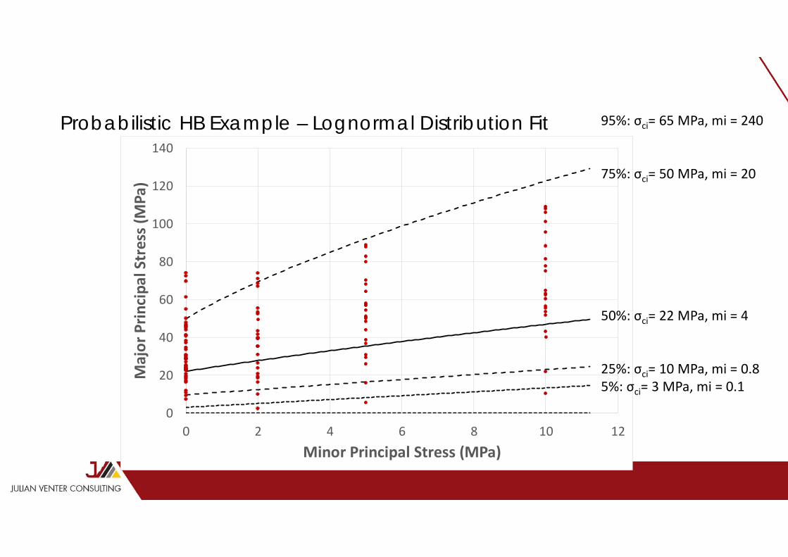
Probabilistic HB Example – Lognormal Distribution Fit
0
20
40
60
80
100
120
140
0 2 4 6 8 10 12
Major Prin
cipa
l Stress (M
Pa)
Minor Principal Stress (MPa)
95%: σci= 65 MPa, mi = 240
75%: σci= 50 MPa, mi = 20
50%: σci= 22 MPa, mi = 4
25%: σci= 10 MPa, mi = 0.85%: σci= 3 MPa, mi = 0.1

0
20
40
60
80
100
120
140
160
180
200
0 2 4 6 8 10 12
Major Prin
cipa
l Stress (M
Pa)
Minor Principal Stress (MPa)
Probabilistic HB Example – Beta Distribution Fit (Satisfies Principle of Maximum Entropy)
95%: σci= 70 MPa, mi = 30
75%: σci= 44 MPa, mi = 13
50%: σci= 29 MPa, mi = 6
25%: σci= 17 MPa, mi = 35%: σci= 7 MPa, mi = 2

Probabilistic HB Example – mi Distributions
0
0.02
0.04
0.06
0.08
0.1
0.12
0.14
0.16
0 10 20 30 40 50
Prob
ability Den
sity Fun
ction
mi
Norm LogNorm Beta
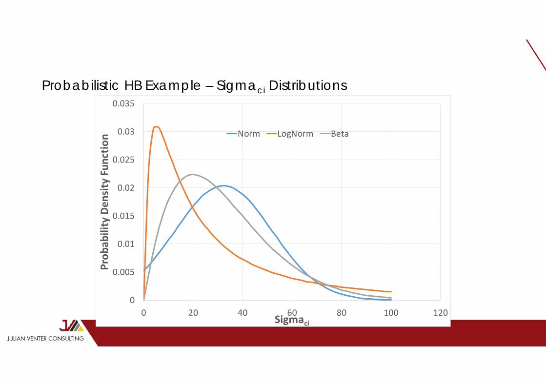
Probabilistic HB Example – Sigmaci Distributions
0
0.005
0.01
0.015
0.02
0.025
0.03
0.035
0 20 40 60 80 100 120
Prob
ability Den
sity Fun
ction
Sigmaci
Norm LogNorm Beta

A Note on Correlation
• For single stage testing it is assumed that mi and Sigmaci is correlated with a coefficient of 1 (i.e. they are really the same variable)
• Using multistage testing the true correlation can be estimated• For this example it is -0.2

A Note on Correlation
0
10
20
30
40
50
60
70
0 5 10 15 20 25 30 35 40
Sigm
aci (MPa)
mi
Correlation Coefficient = ‐0.2

Conventional Multi-Stage Testing Pros and Cons
For• Same sample used at different confinements
• More efficient use of samples• HB curve from single sample• Probabilistic Advantages as presented earlier
Against• Too much damage between stages
• Manual picking of stages imprecise

Servo Controlled Automated Triaxial Machine
• Completely automated testing• Stage end picked based on Poisson’s ratio (0.4 suggested)• More consistent stage transitions• More precise stage yield points• Results much better at simulating single stage testing

Servo Controlled Automated Triaxial Machine

Servo Controlled Automated Triaxial Machine

Servo Controlled Automated Triaxial Machine

Servo Controlled Automated Triaxial Machine
0
50
100
150
200
250
300
350
400
-2000 -1000 0 1000 2000 3000 4000 5000
Axial
Stre
ss (M
Pa)
Strain - µe

Servo Controlled Automated Triaxial Machine

Servo Controlled Automated Triaxial Machine
0
34
68
102
136
170
204
238
272
0 34 68 102 136 170 204 238 272 306
Shea
r Stre
ss M
Pa
Normal Stress MPa
0.4 Poisson's Ratio - Mohr Circle Plot12.01 MPa 24.00 MPa 35.99 MPa 48.00 MPa 59.99 MPa Envelope

Servo Controlled Automated Triaxial Machine
0
53
106
159
212
265
318
371
424
0 53 106 159 212 265 318 371 424 477
Shea
r Stre
ss M
Pa
Normal Stress MPa
Calculated Peak Stress Mohr Circle Plot12.01 MPa 24.00 MPa 35.99 MPa 48.00 MPa 59.99 MPa Envelope

Automated Servo Controlled Multi-Stage Testing Pros and Cons
For• Same sample used at different confinements
• More efficient use of samples• HB curve from single sample• Probabilistic Advantages as presented earlier
• Limited damage between stages• Automated picking of stages
Against• Too much damage between stages
• Manual picking of stages imprecise

Core Log

Slope Design Parameters
0
0.005
0.01
0.015
0.02
0.025
0.03
0.035
0.04
0 20 40 60 80 100 120
Prob
ability Den
sity Fun
ction
GSI
Norm Beta
Average = 41St Dev = 12

Slope Design Parameters
0
0.5
1
1.5
2
2.5
3
3.5
0 0.2 0.4 0.6 0.8 1 1.2 1.4 1.6
Prob
ability Den
sity Fun
ction
mb
Norm Beta
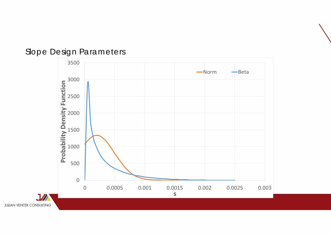
Slope Design Parameters
0
500
1000
1500
2000
2500
3000
3500
0 0.0005 0.001 0.0015 0.002 0.0025 0.003
Prob
ability Den
sity Fun
ction
s
Norm Beta

Slope Design Parameters
0
10
20
30
40
50
60
0.5 0.55 0.6 0.65 0.7
Prob
ability Den
sity Fun
ction
a
Norm Beta

Slope Design Parameters
0
0.0005
0.001
0.0015
0.002
0.0025
0.003
0.0035
0.004
0 100 200 300 400 500 600
Prob
ability Den
sity Fun
ction
c (kPa)
Norm Beta
Average = 164St Dev = 108
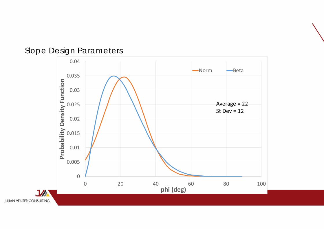
Slope Design Parameters
0
0.005
0.01
0.015
0.02
0.025
0.03
0.035
0.04
0 20 40 60 80 100
Prob
ability Den
sity Fun
ction
phi (deg)
Norm Beta
Average = 22St Dev = 12

Slope Design Parameters – Correlation Coefficients
mi Sci GSI mb s a c phimi 1 -0.20 -0.04 0.79 -0.01 0.12 0.26 0.51Sci 1 0.09 -0.09 0.01 -0.12 0.49 0.48GSI 1 0.42 0.75 -0.96 0.71 0.51mb 1 0.32 -0.36 0.53 0.67s 1 -0.57 0.68 0.32a 1 -0.61 -0.47c 1 0.88phi 1

SV Slope Results - Deterministic
FoS = 1.225

SV Slope – Normal Distribution Inputs
POF = 36%
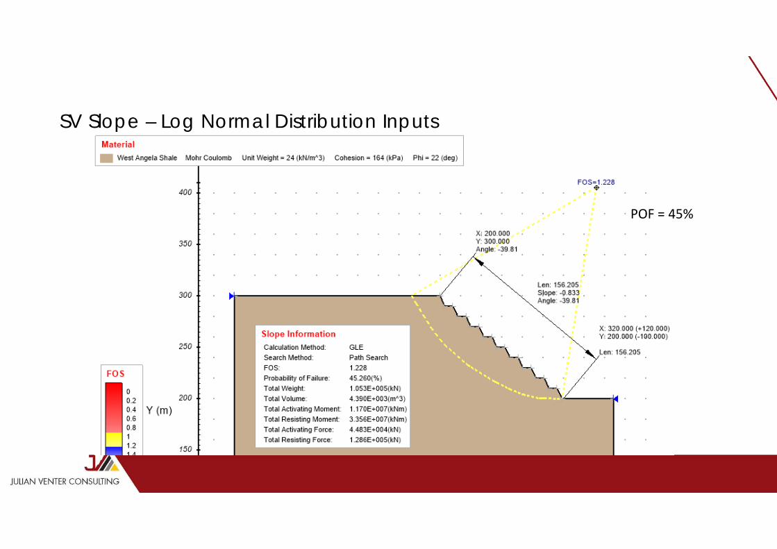
SV Slope – Log Normal Distribution Inputs
POF = 45%

SV Slope – Beta Distribution Inputs
POF = 33%

SV Slope – Spatial Variability

SV Slope – Spatial Variability

SV Slope – 3D

SV Slope – 3D

SV Slope – 3D

SV Slope – 3D

SV Slope – 3D
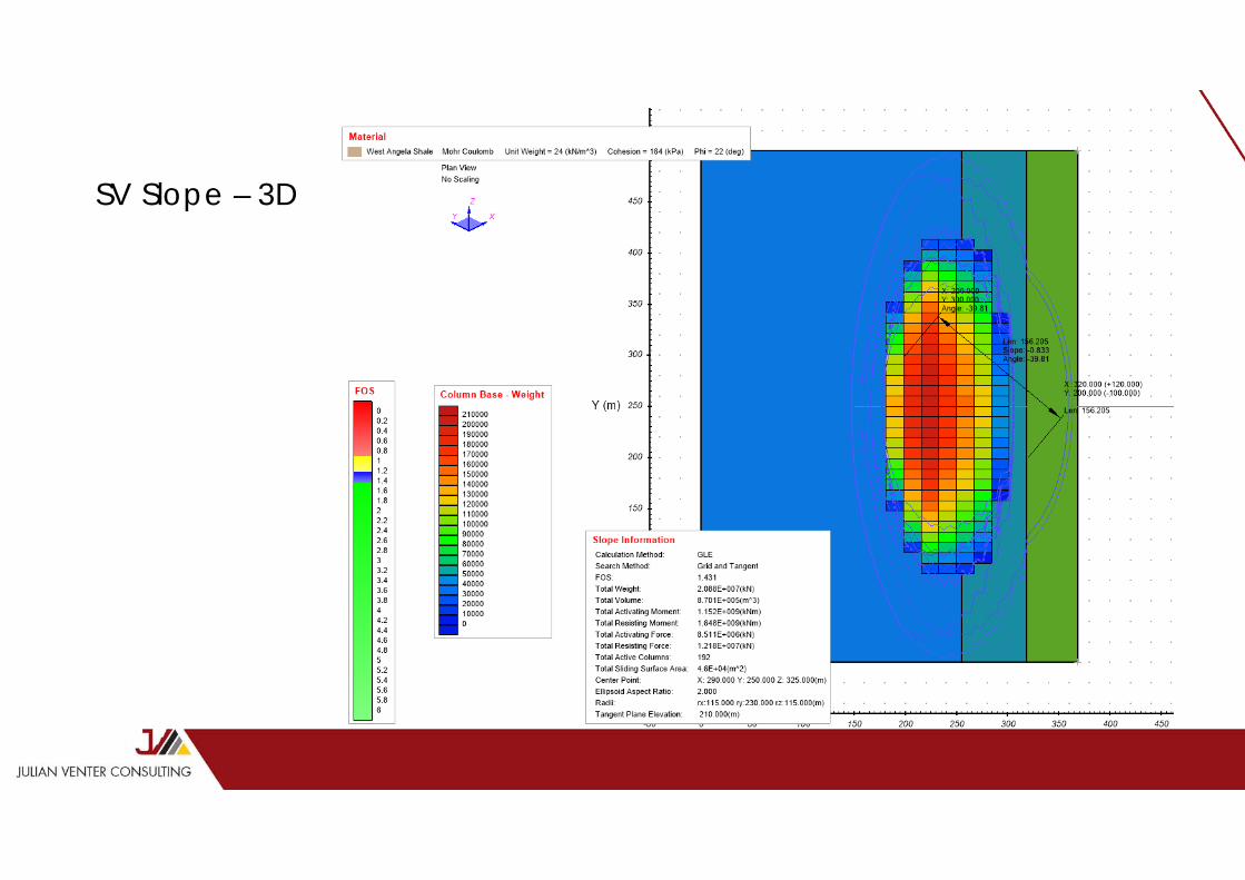
SV Slope – 3D

References
• Grant, E. L., Ireson, W. G., & Leavenworth, R. S. (1990). Principles of Engineering Economy (éd. 8th). Toronto: JohnWiley and Sons.
• Hoek E., 2007. Rock Engineering Course Notes. www.Rocscience.com• Hoek E., Carranza‐Torres C., Corkum B., 2002. Hoek‐Brown Failure Criterion 2002 Edition. www.Rocscience.com
• Harr M.E., 1987. Reliability‐Based Design in Civil Engineering
Recommended