We thank the seminar participants at the Departament d’Economia i d’Història Econòmica, Universitat*
Autònoma de Barcelona. Financial support from the Instituto Valenciano de Investigaciones Económicas (Ivie),is gratefully acknowledged.
University of Valencia.**
PRODUCT QUALITY AND DISTRIBUTION CHANNELS*
Rafael Moner-Colonques, José J. Sempere-Monerrisand Amparo Urbano**
WP-AD 2000-19
Correspondence to R. Moner-Colonques: Universitat de València. Facultad de CC.EE. y EE.,Depto. de Análisis Económico, Campus de los Naranjos, s/n, Edificio Departamental Oriental,46011 Valencia. Tel.: 963 828 246 / E-mail: [email protected].
Editor: Instituto Valenciano de Investigaciones Económicas, S.A.First Edition October 2000.Depósito Legal:V-4118-2000
IVIE working papers offer in advance the results of economic research under way in order toencourage a discussion process before sending them to scientific journals for their finalpublication.
2
PRODUCT QUALITY AND DISTRIBUTION CHANNELS
Rafael Moner-Colonques, José J. Sempere-Monerrisand Amparo Urbano
A B S T R A C T
We introduce strategic behaviour in assigning a certain distribution channel to a productof a particular quality. We propose a variety of models to analyze and study some of thedeterminants of the choice of distribution channels. Taking the Gabszewicz and Thisse's (1979)model as a benchmark, we first study whether there exist strategic incentives for delegation ofsales in a vertically differentiated duopoly. Secondly, product quality is associated with aparticular distribution channel. Finally, the model is extended to account for multi-qualityproduction.
The resulting equilibria of every game depend on the relative market profitability, thedegree of vertical differentiation (i.e. the relative marginal utility of income for quality and thenon-buying option), and hence on the intensity of inter-quality and intra-quality competition.
In all of the games analyzed, delegation appears as an equilibrium action. In the first gameit is a dominant action for both manufacturers. In the second game, at least one of themanufacturers delegates sales. Whether it is one or both crucially depends on market profitabilityfor each quality and the intensity of inter-quality competition. In the third of the games, thesingle-product manufacturer delegates sales at equilibrium whereas the multi-productmanufacturer delegates only one of the qualities. The multi-product manufacturer employswholesale prices together with the decision of not delegating both qualities to optimally combinethe trade-off between the intensity of intra-quality competition and intra-firm competition.
Keywords: vertical differentiation, distribution channels, multi-quality production.
JEL Classification System: D21, L29.
1 Introduction
Our goal is to introduce strategic behaviour in assigning a certain distribu-
tion channel to a product of a particular quality. Also, we wish to contribute
to the study of the determinants of the choice of distribution channels. We
propose a variety of models which allow us to analyze the kind of questions
studied in the literature on distribution systems.
Let us consider the following example to illustrate the issues examined in
this paper. The Spanish ¯rm Basi S.A., located in Barcelona, has got the li-
cence to produce and market the French wear brand Lacoste. Basi produces
two qualities and the little crocodile label, the distinctive sign of Lacoste,
is exclusively attached on the better quality clothes. Lacoste has its own
franchise shops in Spain, where its high-quality clothes are sold. Basi (or
Lacoste if you wish) then faces the decision of which distribution channel
should it employ to sell both their qualities. It would not certainly like to
market clothes with and without the crocodile tag through the same shop
(for reputation reasons). In fact, Basi might even prefer to distribute just
the high-quality or the low-quality wear.
The decision for consumers is not how many jumpers or pairs of trousers
to buy but rather whether they should buy a jumper and, if so, whether it
should be a high-quality jumper (with the crocodile tag and sold in a certain
shop) or a low-quality jumper (without the tag and sold in another shop).
Consumers are unanimous in ranking the quality of jumpers. An important
3
point for a consumer is whether he can a®ord a high-quality jumper, i.e. not
all consumers have the same income. The market described ¯ts as well for
some products in the food and beverage industries, with the growing appear-
ance of private labels. Another relevant aspect in explaining the connection
between product quality and distribution channels is the spreading of on-line
services through the web, in an e®ort of getting hold of medium-high income
consumers.
Therefore, vertical di®erentiation, income disparities, multiproduct qual-
ity and the strategic choice of distribution channels are elements that deserve
joint analysis in order to study their interaction. The demand side takes after
the well-known paper by Gabszewicz and Thisse (1979) and we will proceed
in steps by extending it to account for delegation of sales and multi-quality
production. We will present three multi-stage non-cooperative games played
by two manufacturers to assess whether strategic behaviour may explain an
association between product quality and the distribution channel selected
by the manufacturers. In other words, we aim at analyzing whether product
quality and distribution channels appear endogenously linked as the outcome
of a non-cooperative game.
We will focus on Cournot competition in the last stage of the game. The
contracts that link a manufacturer with its retailer(s) are two-part tari® con-
tracts. There is complete information and quality levels are exogenously
¯xed. Under these assumptions, the resulting equilibria of every game de-
pend on the relative market pro¯tability, the degree of vertical di®erentiation
4
(i.e. the relative marginal utility of income for quality and the non-buying
option), and hence on the intensity of inter-quality and intra-quality compe-
tition.
The literature on vertical relations is quite extensive. The earlier pa-
pers by Vickers (1985) and by Bonanno and Vickers (1988) studied whether
oligopolistic ¯rms had a unilateral strategic incentive to delegate sales to
independent retailers for the homogeneous and di®erentiated products case,
respectively.1 An important question posed in the literature is whether re-
tail distribution should involve the use of exclusive or common retailers,
possibly along with other vertical restraints clauses. Representative papers
coping with issues such as exclusive dealing, common dealership and mar-
ket foreclosure include Bernheim and Whinston (1998), Besanko and Perry
(1993, 1994), Gabrielsen (1996, 1997), Lin (1990) and O'Brien and Sha®er
(1993, 1997). Other papers consider the mutual incentive for a manufacturer-
retailer pairing to enter into exclusive trading relationships (Chang, 1992, and
Dobson and Waterson, 1997). The resulting market structure when retail-
ers are the decisive agents in choosing the distribution channels is studied
by Moner-Colonques, Sempere-Monerris and Urbano (1999). Finally, it is
worth mentioning a number of papers that do consider multidealer distribu-
tion systems. Recent contributions are Rey and Stiglitz (1995), Dobson and
Waterson (1996) and Gabrielsen and S¿rgard (1999).
1An excellent survey on the value of precommitment in vertical chains is Irmen (1998).
5
To the best of our knowledge, vertical di®erentiation, multi-quality pro-
duction and its relation with distribution channels have not yet been com-
bined in a single model.2 To tackle these issues, we proceed gradually. In
Section 2 we set out the benchmark model, a conveniently adapted and ex-
tended version of Gabszewiz and Thisse's (1979) model. Then, we study
whether there exist strategic motives for delegation of sales in a vertically
di®erentiated duopoly (Section 3). The association of product quality and
distribution channels is taken up in Section 4; a model that can be interpreted
as the endogenous selection of quality by the decision to delegate sales. Sec-
tion 5 extends the previous models to account for multi-quality production.
Some concluding remarks close the paper.
We show that in all of the games analyzed, delegation appears as an
equilibrium action. In the ¯rst game, it is a dominant action for both man-
ufacturers, and contrary to the standard ¯ndings in the literature, it is not
always true that a prisoners' dilemma exists. In the second game, we show
that at least one of the manufacturers delegates sales. Whether one or both
manufacturers delegate sales crucially depends on market pro¯tability for
each quality and the intensity of inter-quality competition. In the third of
the games, the single-product manufacturer delegates sales at equilibrium
whereas the multi-product manufacturer delegates only one of the qualities.
2To be fair, there exists an extensive empirical literature on marketing devoted to
study price di®erences in national and private labels, and the role played by distribution
channels. Recent examples of this literature are the papers by Hoch and Banerji (1993),
and Narasimham and Wilcox (1998).
6
Both manufacturers in the former two games and the single-product man-
ufacturer in the third game employ wholesale prices to incentive retailers'
sales. However, we have found that the multi-product manufacturer in the
third game employs wholesale prices together with the decision of not dele-
gating both qualities to optimally combine the trade-o® between the intensity
of intra-quality competition and intra-¯rm competition.
2 The benchmark model
As a benchmark model we will consider an extension of the model that was
initially proposed by Gabszewicz and Thisse (1979). We assume a market
with two manufacturers, manufacturer MH produces a high-quality good
whereas manufacturer ML produces a low-quality good. Both these qualities
are exogenously given. Let T = [0; 1] represent the set of consumers. A
consumer of type t 2 T has an initial income given by R(t) = R1 + R2t,
with R1 > 0 and R2 ¸ 0. All consumers have identical preferences and their
utility function is de¯ned by,
U(0; R(t)) = u0R(t); in case of no purchase, U(H; R(t)¡pH) = uH(R(t)¡pH); if the consumer buys the high-quality product, and U(L; R(t) ¡ pL) =
uL(R(t) ¡ pL); if the low-quality product is bought. The scalars u0; uH and
uL are positive and verify uH > uL > u0 > 0: This means that all consumers
agree that the high-quality product is preferred to the low-quality product
which in turn is preferred to nothing. Purchases are mutually exclusive.
Then, although consumers agree on the quality ranking, each consumer has
a (di®erent) reservation price since they have di®erent income.
7
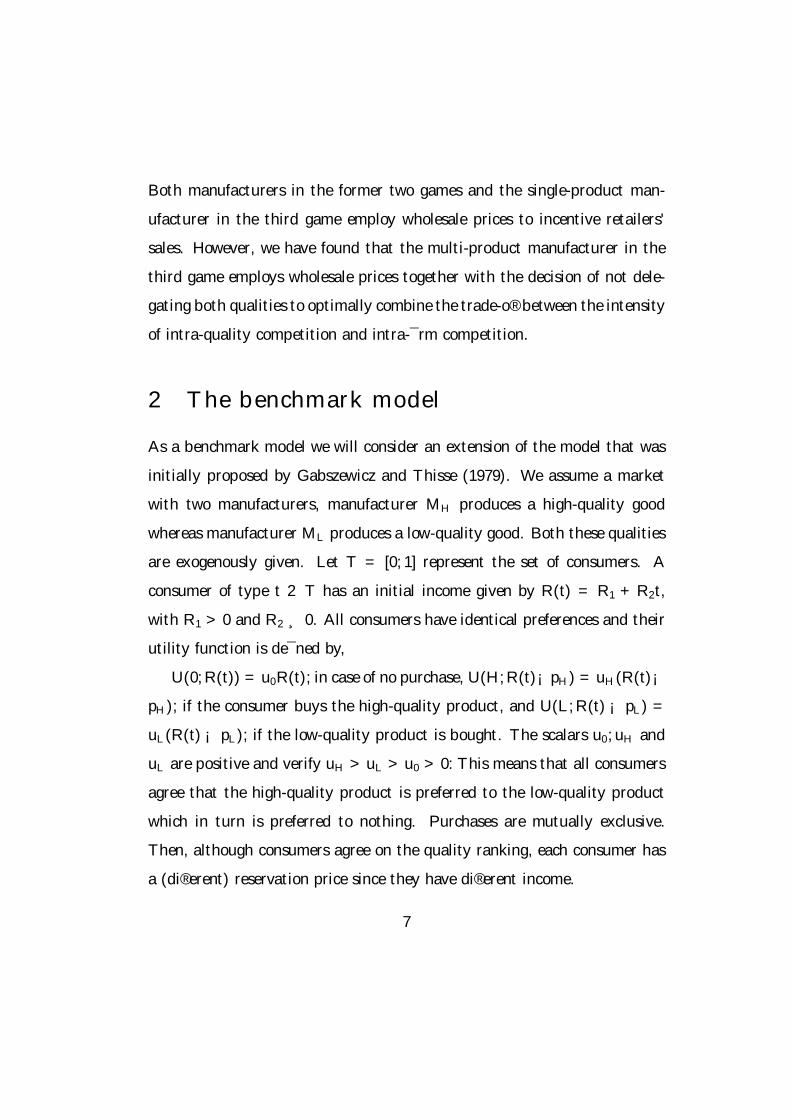
The market T can be partitioned between those consumers who buy the
high-quality product, those who buy the low-quality product and those who
buy neither of them. Note that in Gabszewicz and Thisse's (1979) paper
there are three possible demand con¯gurations corresponding to three dif-
ferent cases: a) both qualities have positive demand but there are unserved
consumers, b) all consumers buy either the high or the low quality product,
and c) only the high quality product is sold. For the sake of the exposition,
we will work with case a). Thus we will require, throughout the analysis,
that the sum of the equilibrium outputs do not exceed one and that both the
high and the low quality outputs be positive.
The demand expressions obtained are,
qL =uHpH ¡ uLpL
(uH ¡ uL)R2¡ uLpL
(uL ¡ u0)R2
qH = 1 ¡ uHpH ¡ uLpL
(uH ¡ uL)R2+
R1
R2
We wish to study quantity competition. By inverting the above demand
system we obtain,
pL =uL ¡ u0
uL(R1 + R2 ¡ R2qH ¡ R2qL) (1)
pH =uH ¡ u0
uH
(R1 + R2) ¡µ
uH ¡ u0
uH
¶R2qH ¡
µuL ¡ u0
uH
¶R2qL (2)
8
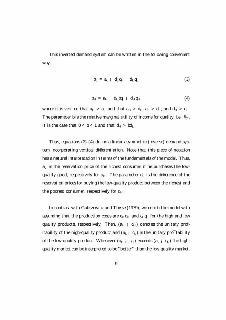
This inverted demand system can be written in the following convenient
way,
pL = aL ¡ dLqH ¡ dLqL (3)
pH = aH ¡ dLbqL ¡ dHqH (4)
where it is veri¯ed that aH > aL and that aH > dH ; aL > dL; and dH > dL.
The parameter b is the relative marginal utility of income for quality, i.e. uL
uH.
It is the case that 0 < b < 1 and that dH > bdL.
Thus, equations (3)-(4) de¯ne a linear asymmetric (inverse) demand sys-
tem incorporating vertical di®erentiation. Note that this piece of notation
has a natural interpretation in terms of the fundamentals of the model. Thus,
aL is the reservation price of the richest consumer if he purchases the low-
quality good, respectively for aH . The parameter dL is the di®erence of the
reservation prices for buying the low-quality product between the richest and
the poorest consumer, respectively for dH .
In contrast with Gabszewicz and Thisse (1979), we enrich the model with
assuming that the production costs are cHqH and cLqL for the high and low
quality products, respectively. Then, (aH ¡ cH) denotes the unitary prof-
itability of the high-quality product and (aL ¡ cL) is the unitary pro¯tability
of the low-quality product. Whenever (aH ¡ cH) exceeds (aL ¡ cL);the high-
quality market can be interpreted to be "better" than the low-quality market.
9
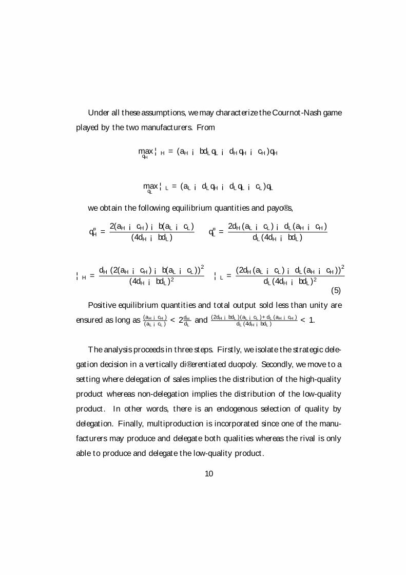
Under all these assumptions, we may characterize the Cournot-Nash game
played by the two manufacturers. From
maxqH
¦H = (aH ¡ bdLqL ¡ dHqH ¡ cH)qH
maxqL
¦L = (aL ¡ dLqH ¡ dLqL ¡ cL)qL
we obtain the following equilibrium quantities and payo®s,
q¤H =
2(aH ¡ cH) ¡ b(aL ¡ cL)
(4dH ¡ bdL)q¤
L =2dH(aL ¡ cL) ¡ dL(aH ¡ cH)
dL(4dH ¡ bdL)
¦H =dH (2(aH ¡ cH) ¡ b(aL ¡ cL))2
(4dH ¡ bdL)2¦L =
(2dH(aL ¡ cL) ¡ dL(aH ¡ cH))2
dL(4dH ¡ bdL)2
(5)
Positive equilibrium quantities and total output sold less than unity are
ensured as long as (aH¡cH)(aL¡cL)
< 2dH
dLand (2dH¡bdL)(aL¡cL)+dL(aH¡cH)
dL(4dH¡bdL)< 1.
The analysis proceeds in three steps. Firstly, we isolate the strategic dele-
gation decision in a vertically di®erentiated duopoly. Secondly, we move to a
setting where delegation of sales implies the distribution of the high-quality
product whereas non-delegation implies the distribution of the low-quality
product. In other words, there is an endogenous selection of quality by
delegation. Finally, multiproduction is incorporated since one of the manu-
facturers may produce and delegate both qualities whereas the rival is only
able to produce and delegate the low-quality product.
10
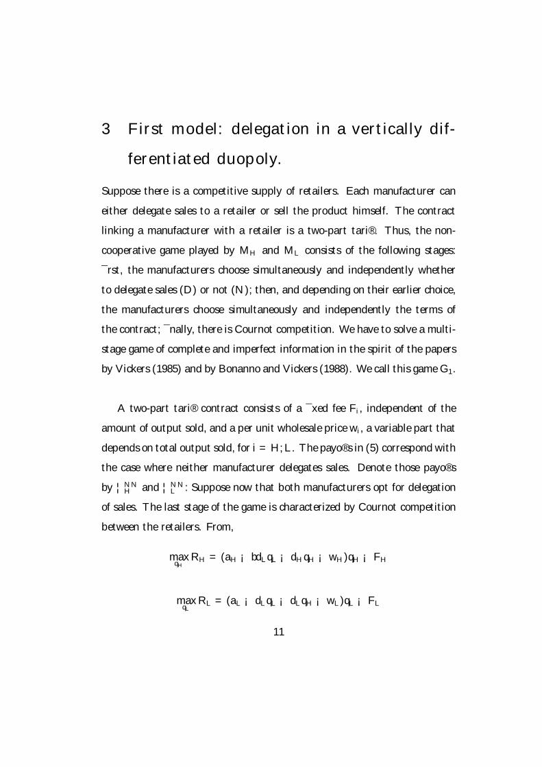
3 First model: delegation in a vertically dif-
ferentiated duopoly.
Suppose there is a competitive supply of retailers. Each manufacturer can
either delegate sales to a retailer or sell the product himself. The contract
linking a manufacturer with a retailer is a two-part tari®. Thus, the non-
cooperative game played by MH and ML consists of the following stages:
¯rst, the manufacturers choose simultaneously and independently whether
to delegate sales (D) or not (N); then, and depending on their earlier choice,
the manufacturers choose simultaneously and independently the terms of
the contract; ¯nally, there is Cournot competition. We have to solve a multi-
stage game of complete and imperfect information in the spirit of the papers
by Vickers (1985) and by Bonanno and Vickers (1988). We call this game G1.
A two-part tari® contract consists of a ¯xed fee Fi, independent of the
amount of output sold, and a per unit wholesale price wi, a variable part that
depends on total output sold, for i = H; L. The payo®s in (5) correspond with
the case where neither manufacturer delegates sales. Denote those payo®s
by ¦NNH and ¦NN
L : Suppose now that both manufacturers opt for delegation
of sales. The last stage of the game is characterized by Cournot competition
between the retailers. From,
maxqH
RH = (aH ¡ bdLqL ¡ dHqH ¡ wH)qH ¡ FH
maxqL
RL = (aL ¡ dLqL ¡ dLqH ¡ wL)qL ¡ FL
11
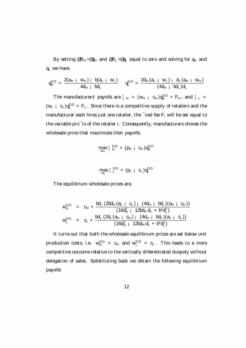
By setting @RH=@qH and @RL=@qL equal to zero and solving for qH and
qL we have,
qDDH =
2(aH ¡ wH) ¡ b(aL ¡ wL)
4dH ¡ bdLqDD
L =2dH(aL ¡ wL) ¡ dL(aH ¡ wH)
(4dH ¡ bdL)dL
The manufacturers' payo®s are ¦H = (wH ¡ cH)qDDH + FH ; and ¦L =
(wL ¡ cL)qDDL + FL. Since there is a competitive supply of retailers and the
manufacturer each hires just one retailer, the ¯xed fee Fi will be set equal to
the variable pro¯ts of the retailer i. Consequently, manufacturers choose the
wholesale price that maximizes their payo®s.
maxwH
¦DDH = (pH ¡ cH)qDD
H
maxwL
¦DDL = (pL ¡ cL)qDD
L
The equilibrium wholesale prices are,
wDDH = cH +
bdL (2bdH(aL ¡ cL) ¡ (4dH ¡ bdL)(aH ¡ cH))
(16d2H ¡ 12bdHdL + b2d2
L)
wDDL = cL +
bdL (2dL(aH ¡ cH) ¡ (4dH ¡ bdL)(aL ¡ cL))
(16d2H ¡ 12bdHdL + b2d2
L)
It turns out that both the wholesale equilibrium prices are set below unit
production costs, i.e. wDDH < cH and wDD
L < cL. This leads to a more
competitive outcome relative to the vertically di®erentiated duopoly without
delegation of sales. Substituting back we obtain the following equilibrium
payo®s
12
¦DDH =
2(2dH ¡ bdL) ((4dH ¡ bdL)(aH ¡ cH) ¡ 2bdH(aL ¡ cL))2
(16d2H ¡ 12bdHdL + b2d2
L)2(6)
¦DDL =
2dH(2dH ¡ bdL) ((4dH ¡ bdL)(aL ¡ cL) ¡ 2dL(aH ¡ cH))2
dL(16d2H ¡ 12bdHdL + b2d2
L)2(7)
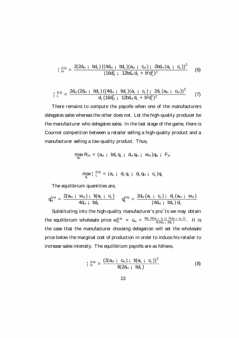
There remains to compute the payo®s when one of the manufacturers
delegates sales whereas the other does not. Let the high-quality producer be
the manufacturer who delegates sales. In the last stage of the game, there is
Cournot competition between a retailer selling a high-quality product and a
manufacturer selling a low-quality product. Thus,
maxqH
RH = (aH ¡ bdLqL ¡ dHqH ¡ wH)qH ¡ FH
maxqL
¦DNL = (aL ¡ dLqL ¡ dLqH ¡ cL)qL
The equilibrium quantities are,
qDNH =
2(aH ¡ wH) ¡ b(aL ¡ cL)
4dH ¡ bdL
qDNL =
2dH(aL ¡ cL) ¡ dL(aH ¡ wH)
(4dH ¡ bdL) dL
Substituting into the high-quality manufacturer's pro¯ts we may obtain
the equilibrium wholesale price wDNH = cH + bdL(b(aL¡cL)¡2(aH¡cH))
4(2dH¡bdL). It is
the case that the manufacturer choosing delegation will set the wholesale
price below the marginal cost of production in order to induce his retailer to
increase sales intensity. The equilibrium payo®s are as follows,
¦DNH =
(2(aH ¡ cH) ¡ b(aL ¡ cL))2
8(2dH ¡ bdL)(8)
13
¦DNL =
((4dH ¡ bdL)(aL ¡ cL) ¡ 2dL(aH ¡ cH))2
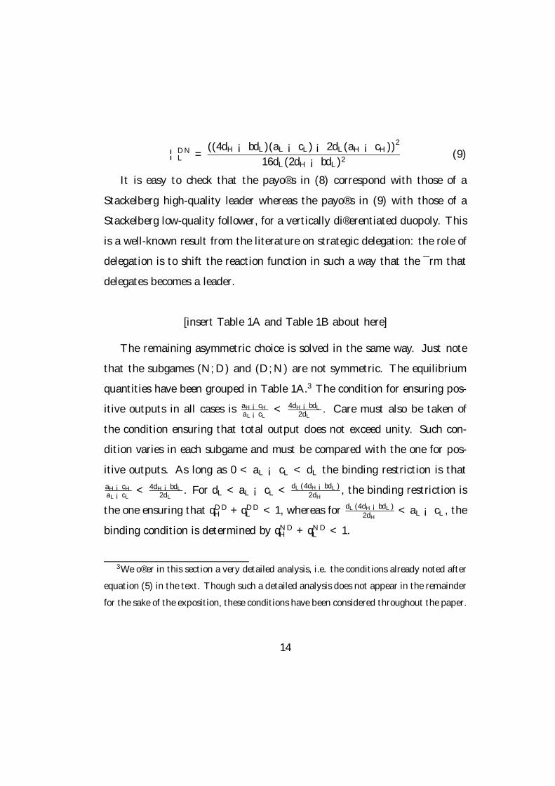
16dL(2dH ¡ bdL)2(9)
It is easy to check that the payo®s in (8) correspond with those of a
Stackelberg high-quality leader whereas the payo®s in (9) with those of a
Stackelberg low-quality follower, for a vertically di®erentiated duopoly. This
is a well-known result from the literature on strategic delegation: the role of
delegation is to shift the reaction function in such a way that the ¯rm that
delegates becomes a leader.
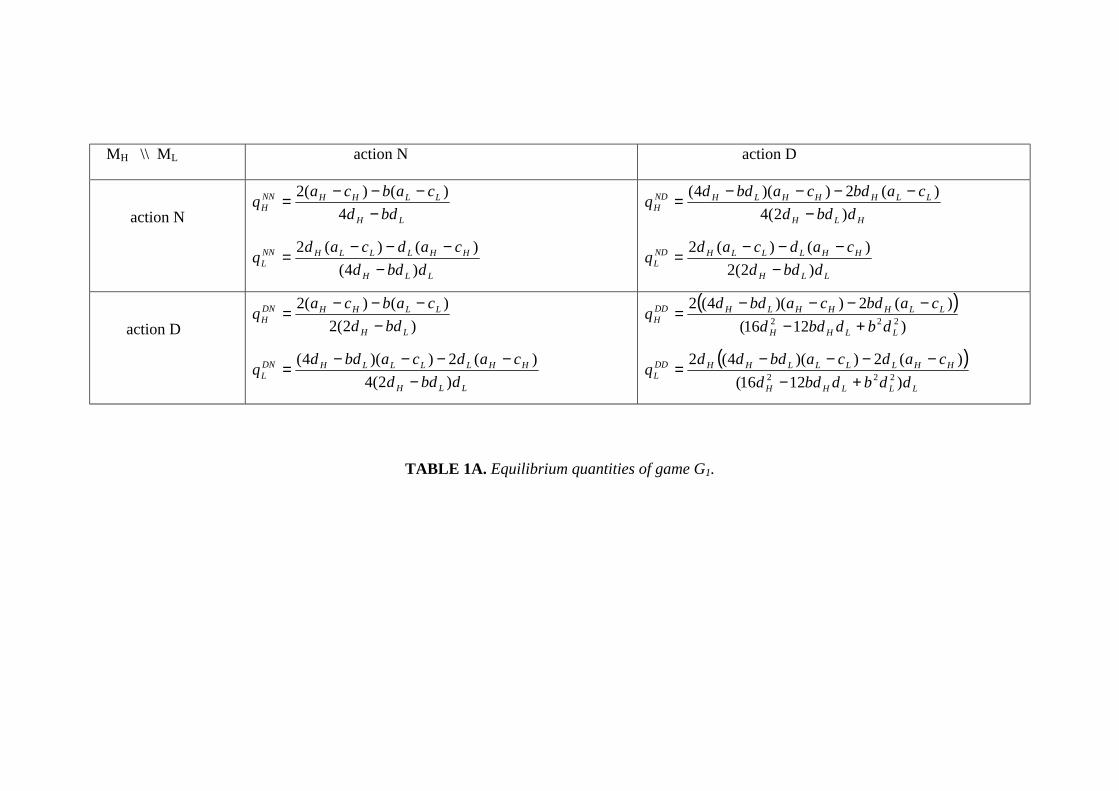
[insert Table 1A and Table 1B about here]
The remaining asymmetric choice is solved in the same way. Just note
that the subgames (N; D) and (D; N) are not symmetric. The equilibrium
quantities have been grouped in Table 1A.3 The condition for ensuring pos-
itive outputs in all cases is aH¡cH
aL¡cL< 4dH¡bdL
2dL. Care must also be taken of
the condition ensuring that total output does not exceed unity. Such con-
dition varies in each subgame and must be compared with the one for pos-
itive outputs. As long as 0 < aL ¡ cL < dL the binding restriction is that
aH¡cH
aL¡cL< 4dH¡bdL
2dL. For dL < aL ¡ cL < dL(4dH¡bdL)
2dH, the binding restriction is
the one ensuring that qDDH + qDD
L < 1, whereas for dL(4dH¡bdL)2dH
< aL ¡ cL, the
binding condition is determined by qNDH + qND
L < 1.
3We o®er in this section a very detailed analysis, i.e. the conditions already noted after
equation (5) in the text. Though such a detailed analysis does not appear in the remainder
for the sake of the exposition, these conditions have been considered throughout the paper.
14
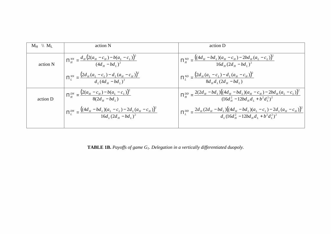
We may then compute the Nash equilibrium of the game G1 (see Table
1B). It turns out that D ("delegation") is a dominant action for each of the
manufacturers. The payo®s in (N; N) and (D; D) are di±cult to compare
and we have resorted to a numerical simulation in order to establish whether
there is a prisoners' dilemma situation. Manufacturer MH is better o® in the
subgame (D; D) than in subgame (N; N) for large enough marginal utility
of income for the high-quality product.
We know from Vickers (1985) that there is a prisoner's dilemma for the
case of a homogeneous product industry. In fact, as pointed out by Irmen
(1998), this result will hold as long as the variables are strategic substitutes.
With strategic complementarity and horizontal product di®erentiation, Bo-
nanno and Vickers (1988) ¯nd that delegation is both in the individual and
the collective interest. What we have found is that there may not be a pris-
oner's dilemma with strategic substitutability and vertical di®erentiation.
The above discussion can be summarized in the following proposition.
Proposition 1 The game G1 has a unique subgame perfect equilibrium. It
has the following properties: a) delegation of sales by both manufacturers is
a dominant action in the ¯rst stage, and b) the equilibrium wholesale prices
are set below the corresponding marginal cost of production.
Thus far, product quality is just associated with a manufacturer. Re-
tailers add nothing to distributing the product and therefore there does not
exist any relation between product quality and distribution channels. What
15
we have shown is the existence of a unilateral incentive to delegate sales in
the presence of vertical di®erentiation and quantity competition.
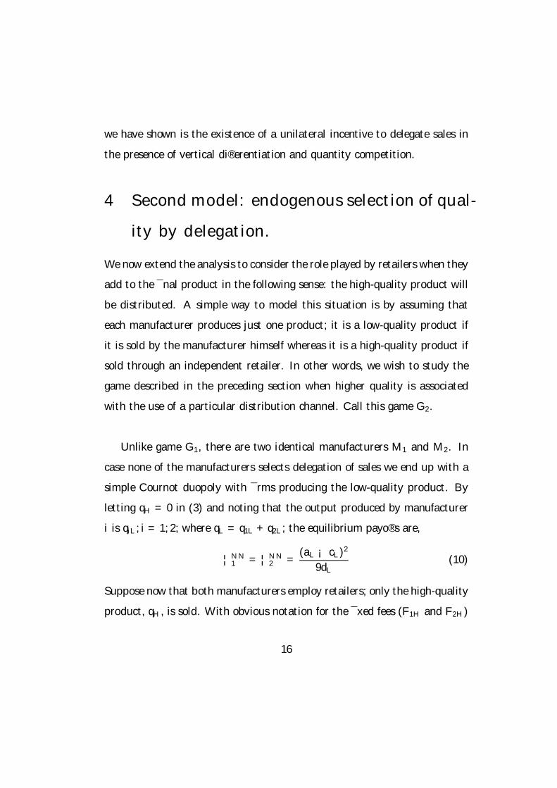
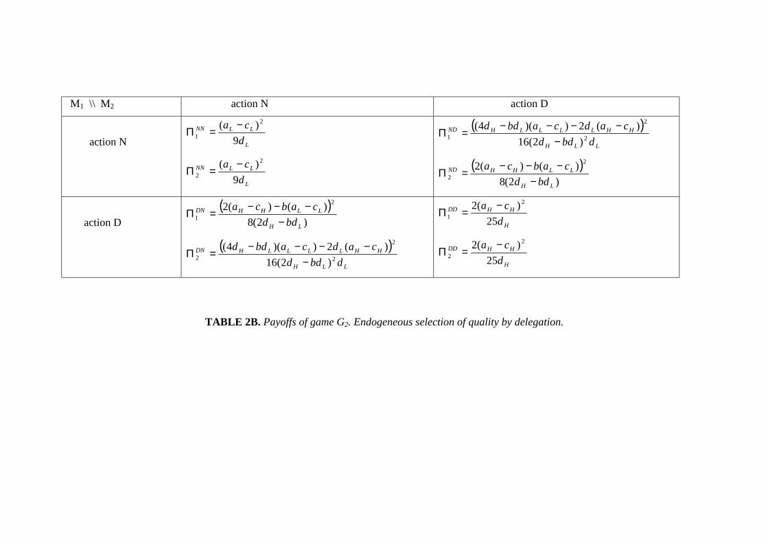
4 Second model: endogenous selection of qual-
ity by delegation.
We now extend the analysis to consider the role played by retailers when they
add to the ¯nal product in the following sense: the high-quality product will
be distributed. A simple way to model this situation is by assuming that
each manufacturer produces just one product; it is a low-quality product if
it is sold by the manufacturer himself whereas it is a high-quality product if
sold through an independent retailer. In other words, we wish to study the
game described in the preceding section when higher quality is associated
with the use of a particular distribution channel. Call this game G2.
Unlike game G1, there are two identical manufacturers M1 and M2. In
case none of the manufacturers selects delegation of sales we end up with a
simple Cournot duopoly with ¯rms producing the low-quality product. By
letting qH = 0 in (3) and noting that the output produced by manufacturer
i is qiL; i = 1; 2; where qL = q1L + q2L; the equilibrium payo®s are,
¦NN1 = ¦NN
2 =(aL ¡ cL)2
9dL
(10)
Suppose now that both manufacturers employ retailers; only the high-quality
product, qH , is sold. With obvious notation for the ¯xed fees (F1H and F2H)
16
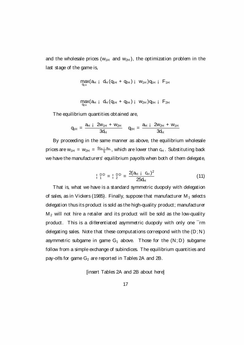
and the wholesale prices (w1H and w2H), the optimization problem in the
last stage of the game is,
maxq1H
(aH ¡ dH(q1H + q2H) ¡ w1H)q1H ¡ F1H
maxq2H
(aH ¡ dH(q1H + q2H) ¡ w2H)q2H ¡ F2H
The equilibrium quantities obtained are,
q1H =aH ¡ 2w1H + w2H
3dH
q2H =aH ¡ 2w2H + w1H
3dH
By proceeding in the same manner as above, the equilibrium wholesale
prices are w1H = w2H = 6cH¡aH
5, which are lower than cH . Substituting back
we have the manufacturers' equilibrium payo®s when both of them delegate,
¦DD1 = ¦DD
2 =2(aH ¡ cH)2
25dH
(11)
That is, what we have is a standard symmetric duopoly with delegation
of sales, as in Vickers (1985). Finally, suppose that manufacturer M1 selects
delegation thus its product is sold as the high-quality product; manufacturer
M2 will not hire a retailer and its product will be sold as the low-quality
product. This is a di®erentiated asymmetric duopoly with only one ¯rm
delegating sales. Note that these computations correspond with the (D; N)
asymmetric subgame in game G1 above. Those for the (N; D) subgame
follow from a simple exchange of subindices. The equilibrium quantities and
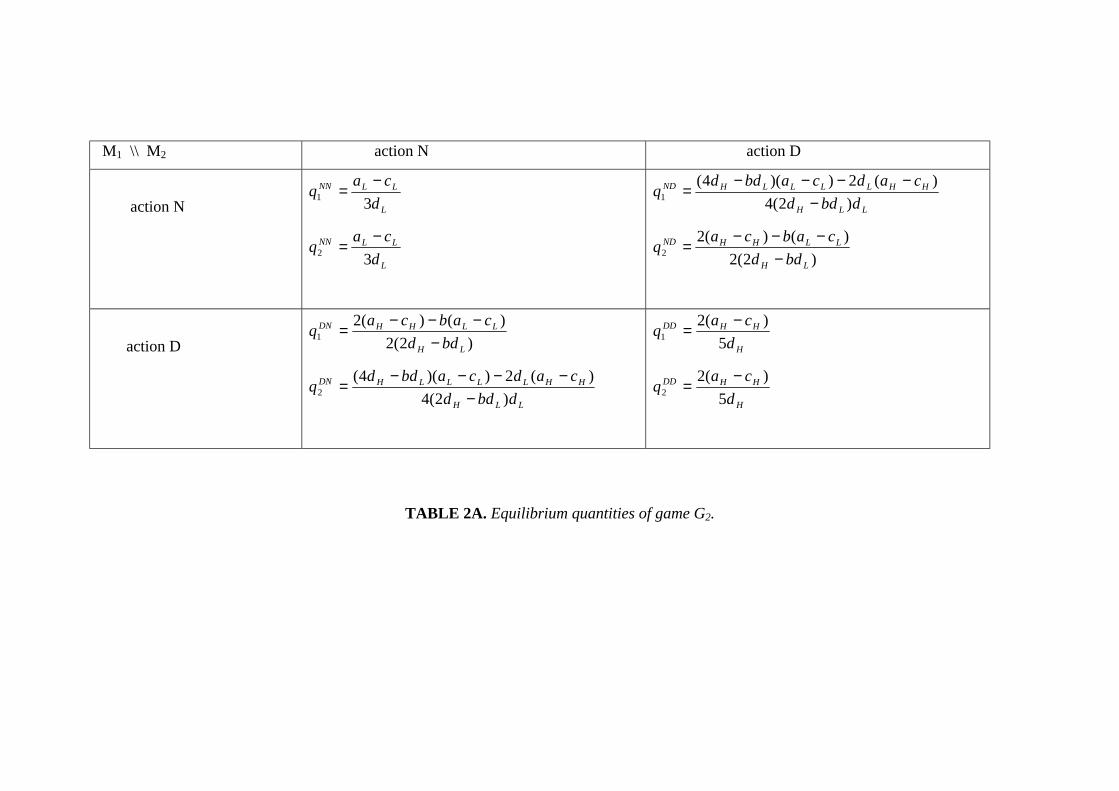
pay-o®s for game G2 are reported in Tables 2A and 2B.
[insert Tables 2A and 2B about here]
17
We make the following assumption dH
dL> cH
cL¸ 1; which means that
the reservation price ratio between purchasing the high and the low-quality
products exceeds the marginal cost of production ratio. It implies that the
pro¯tability ratio between both markets is greater than one, which seems to
be the standard case with more economic content. Under this assumption
the relevant bounds which ensure that all equilibrium outputs in G2 are pos-
itive and that all aggregate outputs are smaller than one are those coming
from qDN2 > 0 and 2qDD
1 < 1; respectively.
Before stating the proposition, it is worth introducing the following useful
notation. First of all, t¡ and t+ are both functions of the fundamentals and
correspond with the bounds ensuring positive outputs and aggregate outputs
less than one, respectively; g+ is also a function of the fundamentals and is
one of the roots satisfying ¦DD1 = ¦ND
1 (or ¦DD2 = ¦DN
2 ): Finally R = R1+R2:
See Appendix A for a more detailed description where a sketch of the proof
is o®ered.
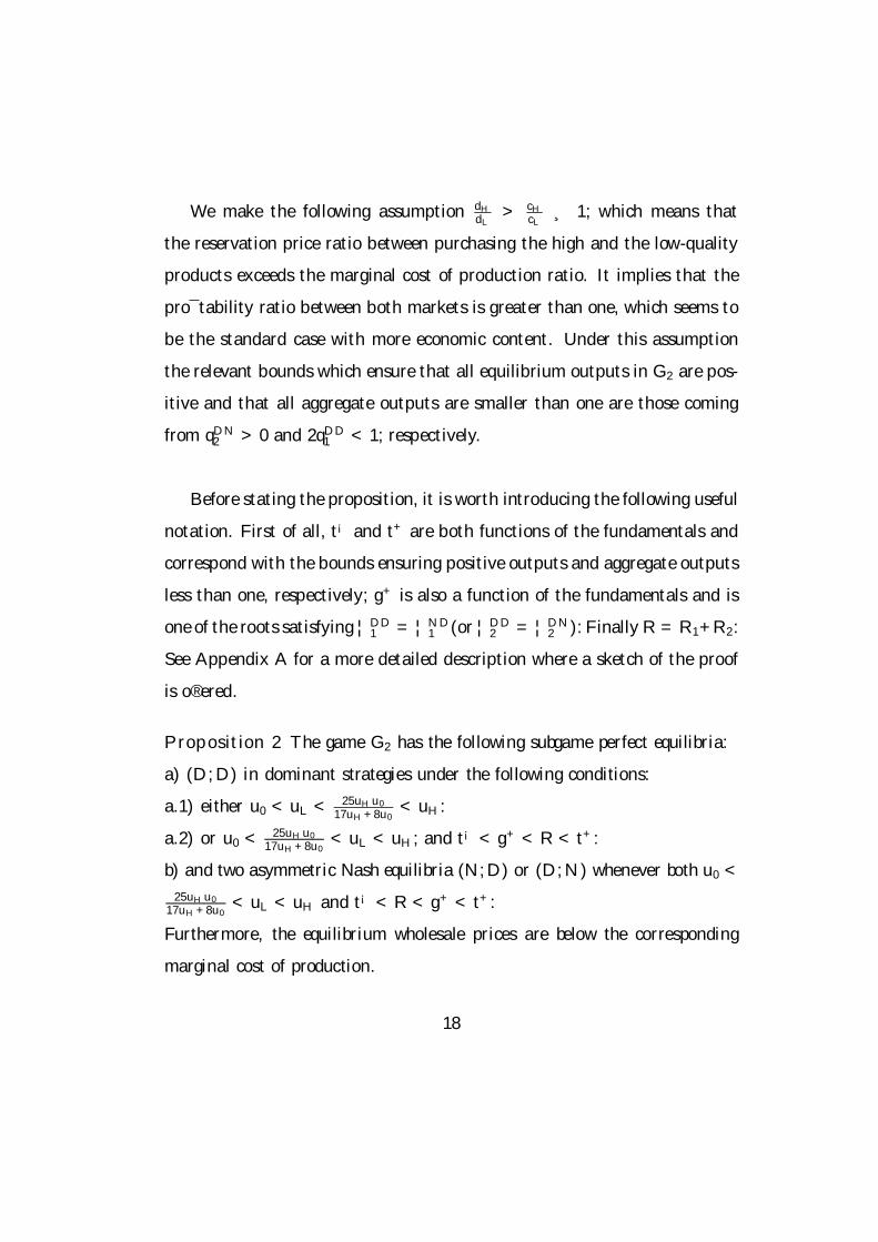
Proposition 2 The game G2 has the following subgame perfect equilibria:
a) (D; D) in dominant strategies under the following conditions:
a.1) either u0 < uL < 25uHu0
17uH+8u0< uH :
a.2) or u0 < 25uHu0
17uH+8u0< uL < uH ; and t¡ < g+ < R < t+:
b) and two asymmetric Nash equilibria (N; D) or (D; N) whenever both u0 <
25uHu0
17uH+8u0< uL < uH and t¡ < R < g+ < t+:
Furthermore, the equilibrium wholesale prices are below the corresponding
marginal cost of production.
18
Delegation, by setting w < c, is an action employed by manufacturers to
induce a higher sales e®ort from retailers. This would be the only e®ect, a
(purely) strategic one, to be considered if product quality and the choice of
distribution channel were not related with each other. Here, in contrast with
the game presented in the previous section, the high-quality product is exclu-
sively sold through retailers. Consequently, the manufacturers' choice must
contemplate a further feature associated with competition intensity. This
e®ect is to be confronted with the one stemming from market pro¯tability,
that is, from how much pro¯table is the high-quality market compared with
the low-quality market. Notice that the equilibrium in dominant strategies
(D; D) implies a homogeneous duopoly in the high-quality product, while the
asymmetric Nash equilibria suppose that a duopoly with di®erent qualities
shows up. Whether one or the other appears depends most importantly on
the relative size among the marginal utility of income from buying either of
the qualities and also that from not buying.
When uL is close to u0, this means that consumers do not value much the
consumption of the low-quality product and, in spite of the high degree of
vertical product di®erentiation, manufacturers delegate sales for pro¯tabil-
ity reasons. In other words, the pro¯ts e®ect more than compensates for
the higher competition intensity under a duopoly in the high-quality market.
Alternatively, when uL is far from u0 the degree of vertical di®erentiation is
low. Provided that competition is rather intense, an additional condition is
needed to ensure the above mentioned equilibrium: it is required that con-
sumers hold enough income. Otherwise a duopoly with both qualities, and
19
hence with di®erent distribution channels, will arise.
5 Third model: multi-quality production and
distribution channels.
We now permit one of the manufacturers, say manufacturer one, to be a mul-
tiproduct ¯rm and choose the distribution pattern accordingly. In particular,
it may either: a) produce and sell himself both the high and the low-quality
products (action N), b) or hire a retailer for distributing the high-quality
product, and sell himself the low-quality one (action H), c) or the reverse of
b (action L), d) or delegate the sales of both qualities to independent and dif-
ferent retailers (action A). The rival manufacturer remains a single-product
¯rm producing the low-quality product and also chooses the way it will be
distributed, either sold by the manufacturer itself (action N) or through a
retailer (action D).
The delegation of sales of both qualities is assumed to take place through
di®erent retailers (as the example in the introduction). This brings new el-
ements into the analysis. With multi-quality production and regardless of
the distribution channel, there appear three outputs in the market, namely
the high-quality product o®ered by the multiproduct ¯rm, qHM , the low-
quality product o®ered by the same ¯rm, qLM , and ¯nally the low-quality
product o®ered by the rival single-product ¯rm, qLU . Thus, we may iden-
20
tify inter-quality competition (between qHM and both qLM and qLU), intra-
quality competition (between qLM and qLU) and intra-¯rm competition (be-
tween qHM and qLM). Therefore, the choice of the distribution channel is
a means of controlling for intra-¯rm competition. For example, when the
multiproduct ¯rm decides not to delegate sales at all, it directly internalizes
intra-¯rm competition. Under delegation of both qualities through di®er-
ent retailers, the intensity of intra-¯rm competition is maximal. However,
the multi-product ¯rm may use the wholesale prices to control for it. Ad-
ditionally, there is competition among manufacturers and then, depending
on market pro¯tability, inter or intra-quality competition will prevail one
upon the other. The interaction of these elements will determine the equi-
librium choice by manufacturers and, consequently, the distribution channel
associated with a particular quality in the presence of a multi-product man-
ufacturer.
Consider the following game, G3. In the ¯rst stage, manufacturers choose
simultaneously and independently the distribution pattern. As mentioned
above, the multiproduct manufacturer chooses an action from the set fN; H; L; Agand the single-product manufacturer chooses an action from the set fN; Dg :
In the second stage, manufacturers choose the terms of the two-part tar-
i® contract, whenever appropriate. In the third stage, all the sellers face
the inverse demand system: pL = aL ¡ dL(qHM + qLM + qLU); pH = aH ¡bdL(qLM + qLU) ¡ dHqHM ; and compete µa la Cournot. Given the ¯rst stage
manufacturers' choice we may study eight di®erent subgames with a di®erent
number of independent sellers at the third stage of the game. For example, in
21
the (H; D) ¡subgame there are three independent sellers: the multi-product
manufacturer selling the low-quality product and two di®erent retailers; while
in the (N; D)¡subgame there are only two: the multi-product manufacturer
and the retailer selling the low-quality product supplied by the single-product
manufacturer. The equilibrium outputs and manufacturers' payo®s for each
of the subgames are presented in appendix B. Before describing the subgame
perfect equilibrium of G3 , we present several partial results, which are proven
in appendix C:
Lemma 1 Delegation is a dominant action for the single-product ¯rm and
it always sets the wholesale price below marginal cost.
The second partial result concerns the equilibrium wholesale prices for the
multi-product manufacturer now focusing on the subgames generated when
the rival manufacturer delegates sales. It is interesting to identify conditions
under which the equilibrium wholesale prices are set below or above the
corresponding marginal cost. Two cases are distinguished. In one of them
the relative pro¯tability ratio does not play any role, the relative position of
the three marginal utilities of income is the key condition. In the second, a
further condition on the size of the relative pro¯tability ratio is required.
Proposition 3 If either i) 53
u0 < uL and uH < '+(u0; uL) and irrespectively
of the size of the relative pro¯tability ratio,
or ii) if 53
u0 < uL and '+(u0; uL) < uH, or if uL < 53
u0 and 8uH; and the rel-
ative pro¯tability ratio is big enough (i.e. aH¡cH
aL¡cL> B ´ 4d2
H¡2b(1¡3b)dHdL¡2b3d2L
dL(2(1+4b)dH¡b(1+3b)dL)>
22
1), then:
a) in the HD-subgame, wHDHM < cH.
b) in the LD-subgame, wLDLM > cL.
c) in the AD-subgame, wADHM < cH and wAD
LM > cL.
The opposite to a), b),and c) happens in part ii) when 1 < aH¡cH
aL¡cL< B:
The result of game G3 is the content of the following proposition,
Proposition 4 The game G3 exhibits two equilibria. In both of them the
single-product manufacturer delegates sales while the multi-product manufac-
turer delegates only one of the qualities. The quality delegated is a function of
the pro¯tability ratio of both markets. The high quality is delegated whenever
the pro¯tability ratio of both markets is big enough (i.e. aH¡cH
aL¡cL> maxf1; Bg);
the low quality is delegated otherwise. Furthermore, the wholesale prices es-
tablished by manufacturers at the equilibrium path are set below the corre-
sponding marginal costs.
Proof: See Appendix C.
To understand the meaning of a big enough pro¯tability ratio note that
part i) in Proposition 3 speci¯es the conditions under which maxf1; Bg = 1
and therefore, the relative pro¯tability ratio trivially satis¯es that condi-
tion, the high-quality market is more pro¯table than the low-quality market.
This happens when uL and uH are rather close to each other (intense inter-
quality competition) and uL is relatively far from u0. However, in part ii)
maxf1; Bg = B and therefore we need the high-quality market to be much
more pro¯table than the low-quality market. This happens either if there is
23
a low degree of inter-quality competition, or if consumers do not value much
the purchase of the low-quality product.
Let us see the intuition behind these results. We begin by recalling the
bottomline from the above games G1 and G2: delegation of sales will take
place no matter whether product quality is associated ab initio with a partic-
ular distribution channel. Then, with a multi-product manufacturer, it seems
natural to consider a game in which it has only got two ¯rst-stage actions,
N and A. In that simpler model, the equilibrium obtained would entail del-
egation by both manufacturers, and such equilibrium would be in dominant
strategies. As noted above, intra-¯rm competition is maximal. One wonders
whether the multi-product manufacturer could do better by only delegating
the sales of one of the products since, by Lemma 1, the single-product man-
ufacturer always delegates sales.
There are several forces at play. One of them has to do with how large
is the relative pro¯tability ratio. Also, the multi-product manufacturer must
consider the di®erent types of quality competition noting that now it has two
instruments at hand: ¯rstly, the wholesale price and, secondly, the channel
for each of the qualities.
Suppose we are in a heavily high-quality oriented situation, that is, the
ratio (aH ¡ cH)=(aL ¡ cL) is very large. If the multi-product manufacturer
delegated the sales of both qualities, then it would use the wholesale prices to
control for intra-¯rm competition. As stated in part c of Proposition 3, just
24
the wholesale price of the high-quality product is set below the corresponding
marginal cost of production. The opposite happens with the low-quality
product but note that it would be sold at a less competitive price than the
rival's. Thus, the multi-product manufacturer, by choosing to delegate only
the sales of the high-quality product, achieves two things. In the ¯rst place, it
induces a higher sales e®ort from his retailer in the high-quality market, which
is very pro¯table. Besides, it is able to compensate for the internalization
loss of intra-product market competition when it delegates both qualities to
independent retailers, thus avoiding the competitive disadvantage associated
with wADLM > cL. We may conclude that, at equilibrium, the multi-product
manufacturer optimally combines the trade-o® between the intensity of intra-
quality competition and intra-¯rm competition. A parallel reasoning applies
when aH ¡ cH is not too large relative to aL ¡ cL and where only the sales of
the low-quality product are delegated at equilibrium. Presumably, we would
have to allude to cost advantages in joint distribution to have both qualities
delegated.
6 Concluding remarks
We have proposed a variety of non-cooperative multi-stage games to ana-
lyze whether product quality and distribution channels appear endogenously
linked as equilibrium outcomes. The demand side of the benchmark model
is that of Gabszewicz and Thisse (1979). Thus, the possible determinants
in explaining the relation between product quality and distribution channels
are the (exogenous) quality levels, income levels, relative market pro¯tability,
25
the use of di®erent channels and multi-quality production.
The theoretical analysis proceeds in steps. The ¯rst setting, a direct
extension of Gabszewicz and Thisse (1979), allows us to show that delega-
tion is the unique subgame perfect equilibrium in dominant strategies for
single-product manufacturers, each one producing a vertically di®erentiated
product. Then, delegation of sales is associated with the choice and distri-
bution of the high-quality product. Delegation of sales by at least one of the
manufacturers is found at equilibrium.
Finally, we have enriched the model by considering a multi-quality manu-
facturer ¯nding that there is a unilateral incentive to delegate sales. Further-
more, the multi-quality manufacturer never sets both equilibrium wholesale
prices below the corresponding marginal costs of production. Two ques-
tions are worth analyzing: a) to widen the set of strategies available to the
multi-quality manufacturer, and b) to allow retailers to introduce and mar-
ket a private label. Concerning a), we have found that the multi-product
manufacturer faces a trade-o® between the internalization of intra-¯rm com-
petition and their control through wholesale prices. In fact, it never delegates
the sales of both qualities. Concerning b), note that it has been documented
that a national brand manufacturer does not typically market two qualities
through the same retailer; a second "private label" is introduced by retailers.
This is left for future research.
26
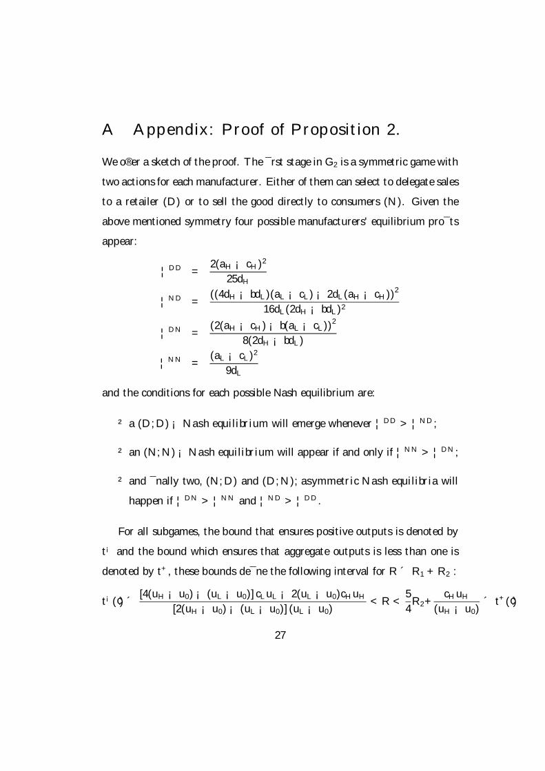
A Appendix: Proof of Proposition 2.
We o®er a sketch of the proof. The ¯rst stage in G2 is a symmetric game with
two actions for each manufacturer. Either of them can select to delegate sales
to a retailer (D) or to sell the good directly to consumers (N). Given the
above mentioned symmetry four possible manufacturers' equilibrium pro¯ts
appear:
¦DD =2(aH ¡ cH)2
25dH
¦ND =((4dH ¡ bdL)(aL ¡ cL) ¡ 2dL(aH ¡ cH))2
16dL(2dH ¡ bdL)2
¦DN =(2(aH ¡ cH) ¡ b(aL ¡ cL))2
8(2dH ¡ bdL)
¦NN =(aL ¡ cL)2
9dL
and the conditions for each possible Nash equilibrium are:
² a (D; D) ¡ Nash equilibrium will emerge whenever ¦DD > ¦ND;
² an (N; N) ¡ Nash equilibrium will appear if and only if ¦NN > ¦DN ;
² and ¯nally two, (N; D) and (D; N); asymmetric Nash equilibria will
happen if ¦DN > ¦NN and ¦ND > ¦DD.
For all subgames, the bound that ensures positive outputs is denoted by
t¡ and the bound which ensures that aggregate outputs is less than one is
denoted by t+, these bounds de¯ne the following interval for R ´ R1 + R2 :
t¡(¢) ´ [4(uH ¡ u0) ¡ (uL ¡ u0)] cLuL ¡ 2(uL ¡ u0)cHuH
[2(uH ¡ u0) ¡ (uL ¡ u0)] (uL ¡ u0)< R <
5
4R2+
cHuH
(uH ¡ u0)´ t+(¢)
27
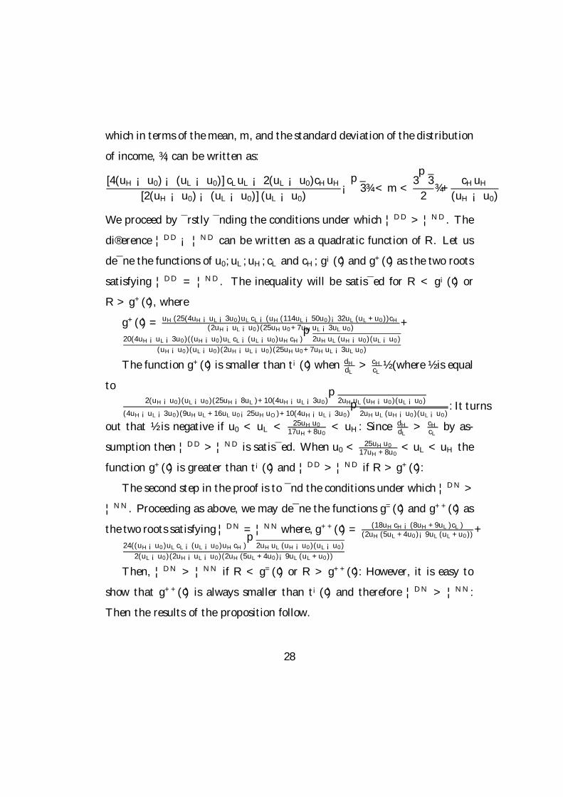
which in terms of the mean, m, and the standard deviation of the distribution
of income, ¾; can be written as:
[4(uH ¡ u0) ¡ (uL ¡ u0)] cLuL ¡ 2(uL ¡ u0)cHuH
[2(uH ¡ u0) ¡ (uL ¡ u0)] (uL ¡ u0)¡
p3¾ < m <
3p
3
2¾+
cHuH
(uH ¡ u0)
We proceed by ¯rstly ¯nding the conditions under which ¦DD > ¦ND. The
di®erence ¦DD ¡ ¦ND can be written as a quadratic function of R. Let us
de¯ne the functions of u0; uL; uH ; cL and cH ; g¡(¢) and g+(¢) as the two roots
satisfying ¦DD = ¦ND. The inequality will be satis¯ed for R < g¡(¢) or
R > g+(¢), where
g+(¢) = uH(25(4uH¡uL¡3u0)uLcL¡(uH(114uL¡50u0)¡32uL(uL+u0))cH
(2uH¡uL¡u0)(25uHu0+7uHuL¡3uLu0)+
20(4uH¡uL¡3u0)((uH¡u0)uLcL¡(uL¡u0)uHcH)p
2uHuL(uH¡u0)(uL¡u0)
(uH¡u0)(uL¡u0)(2uH¡uL¡u0)(25uHu0+7uHuL¡3uLu0)
The function g+(¢) is smaller than t¡(¢) when dH
dL> cH
cL½ (where ½ is equal
to2(uH¡u0)(uL¡u0)(25uH¡8uL)+10(4uH¡uL¡3u0)
p2uHuL(uH¡u0)(uL¡u0)
(4uH¡uL¡3u0)(9uHuL+16uLu0¡25uHuO)+10(4uH¡uL¡3u0)p
2uHuL(uH¡u0)(uL¡u0): It turns
out that ½ is negative if u0 < uL < 25uHu0
17uH+8u0< uH : Since dH
dL> cH
cLby as-
sumption then ¦DD > ¦ND is satis¯ed. When u0 < 25uHu0
17uH+8u0< uL < uH the
function g+(¢) is greater than t¡(¢) and ¦DD > ¦ND if R > g+(¢):The second step in the proof is to ¯nd the conditions under which ¦DN >
¦NN . Proceeding as above, we may de¯ne the functions g=(¢) and g++(¢) as
the two roots satisfying ¦DN = ¦NN where, g++(¢) = (18uHcH¡(8uH+9uL)cL)(2uH(5uL+4u0)¡9uL(uL+u0))
+
24((uH¡u0)uLcL¡(uL¡u0)uHcH)p
2uHuL(uH¡u0)(uL¡u0)
2(uL¡u0)(2uH¡uL¡u0)(2uH(5uL+4u0)¡9uL(uL+u0))
Then, ¦DN > ¦NN if R < g=(¢) or R > g++(¢): However, it is easy to
show that g++(¢) is always smaller than t¡(¢) and therefore ¦DN > ¦NN :
Then the results of the proposition follow.
28
B Appendix: G3 Subgame Equilibrium Out-
comes.
The manufacturers' ¯rst stage action choice gives rise to eight di®erent sub-
games. This appendix displays the equilibrium outputs, wholesale prices
(when appropriate) and the manufacturers' payo®s for each of them. The
notation is:
qzv or wz
v denotes the equilibrium output or wholesale price, respectively,
of good v in the z¡ subgame, where v 2 V = fHM; LM; LUg and z 2 Z =
fN; H; L; Ag £ fN; Dg.
¦zi denotes the equilibrium payo® to manufacturer i in the z¡ subgame,
where i 2 I = fM; Ug:
29
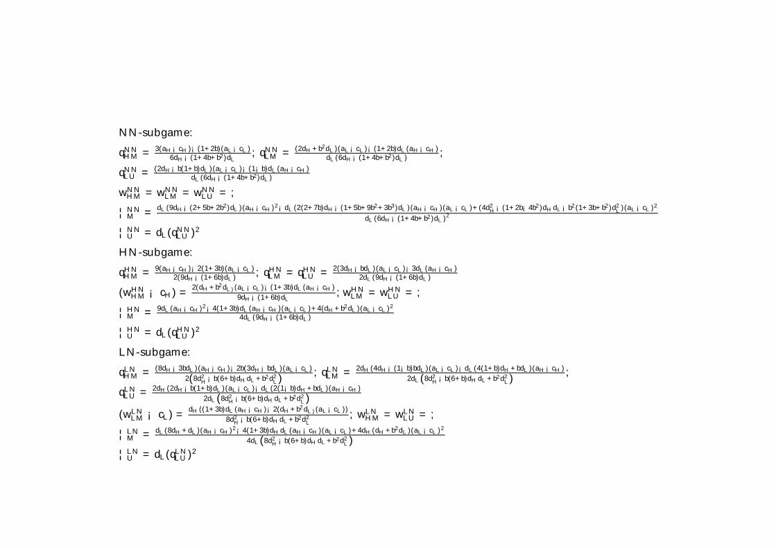
NN-subgame:
qNNHM = 3(aH¡cH)¡(1+2b)(aL¡cL)
6dH¡(1+4b+b2)dL; qNN
LM = (2dH+b2dL)(aL¡cL)¡(1+2b)dL(aH¡cH)dL(6dH¡(1+4b+b2)dL)
;
qNNLU = (2dH¡b(1+b)dL)(aL¡cL)¡(1¡b)dL(aH¡cH)
dL(6dH¡(1+4b+b2)dL)
wNNHM = wNN
LM = wNNLU = ;
¦NNM =
dL(9dH¡(2+5b+2b2)dL)(aH¡cH)2¡dL(2(2+7b)dH¡(1+5b+9b2+3b3)dL)(aH¡cH)(aL¡cL)+(4d2H¡(1+2b¡4b2)dHdL¡b2(1+3b+b2)d2
L)(aL¡cL)2
dL(6dH¡(1+4b+b2)dL)2
¦NNU = dL(qNN
LU )2
HN-subgame:
qHNHM = 9(aH¡cH)¡2(1+3b)(aL¡cL)
2(9dH¡(1+6b)dL); qHN
LM = qHNLU = 2(3dH¡bdL)(aL¡cL)¡3dL(aH¡cH)
2dL(9dH¡(1+6b)dL)
(wHNHM ¡ cH) =
2(dH+b2dL)(aL¡cL)¡(1+3b)dL(aH¡cH)
9dH¡(1+6b)dL; wHN
LM = wHNLU = ;
¦HNM = 9dL(aH¡cH)2¡4(1+3b)dL(aH¡cH)(aL¡cL)+4(dH+b2dL)(aL¡cL)2
4dL(9dH¡(1+6b)dL)
¦HNU = dL(qHN
LU )2
LN-subgame:
qLNHM = (8dH¡3bdL)(aH¡cH)¡2b(3dH¡bdL)(aL¡cL)
2(8d2H
¡b(6+b)dHdL+b2d2L)
; qLNLM = 2dH(4dH¡(1¡b)bdL)(aL¡cL)¡dL(4(1+b)dH+bdL)(aH¡cH)
2dL(8d2H
¡b(6+b)dHdL+b2d2L)
;
qLNLU = 2dH(2dH¡b(1+b)dL)(aL¡cL)¡dL(2(1¡b)dH+bdL)(aH¡cH)
2dL(8d2H¡b(6+b)dHdL+b2d2
L)
(wLNLM ¡ cL) =
dH((1+3b)dL(aH¡cH)¡2(dH+b2dL)(aL¡cL))
8d2H¡b(6+b)dHdL+b2d2
L; wLN
HM = wLNLU = ;
¦LNM = dL(8dH+dL)(aH¡cH)2¡4(1+3b)dHdL(aH¡cH)(aL¡cL)+4dH(dH+b2dL)(aL¡cL)2
4dL(8d2H¡b(6+b)dHdL+b2d2
L)
¦LNU = dL(qLN
LU )2
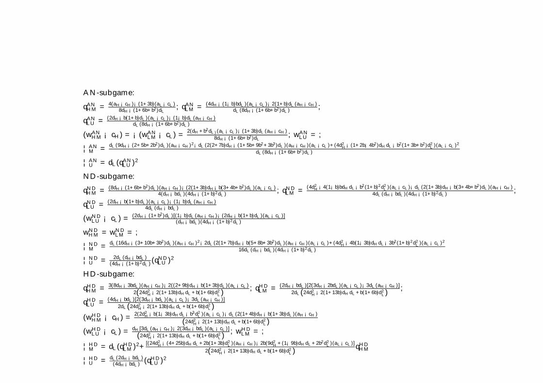
AN-subgame:
qANHM = 4(aH¡cH)¡(1+3b)(aL¡cL)
8dH¡(1+6b+b2)dL; qAN
LM = (4dH¡(1¡b)bdL)(aL¡cL)¡2(1+b)dL(aH¡cH)dL(8dH¡(1+6b+b2)dL)
;
qANLU = (2dH¡b(1+b)dL)(aL¡cL)¡(1¡b)dL(aH¡cH)
dL(8dH¡(1+6b+b2)dL)
(wANHM ¡ cH) = ¡(wAN
LM ¡ cL) =2(dH+b2dL)(aL¡cL)¡(1+3b)dL(aH¡cH)
8dH¡(1+6b+b2)dL; wAN
LU = ;¦AN
M =dL(9dH¡(2+5b+2b2)dL)(aH¡cH)2¡dL(2(2+7b)dH¡(1+5b+9b2+3b3)dL)(aH¡cH)(aL¡cL)+(4d2
H¡(1+2b¡4b2)dHdL¡b2(1+3b+b2)d2L)(aL¡cL)2
dL(8dH¡(1+6b+b2)dL)
¦ANU = dL(qAN
LU )2
ND-subgame:
qNDHM = (8dH¡(1+6b+b2)dL)(aH¡cH)¡(2(1+3b)dH¡b(3+4b+b2)dL)(aL¡cL)
4(dH¡bdL)(4dH¡(1+b)2dL); qND
LM =(4d2
H¡4(1¡b)bdHdL¡b2(1+b)2d2L)(aL¡cL)¡dL(2(1+3b)dH¡b(3+4b+b2)dL)(aH¡cH)
4dL(dH¡bdL)(4dH¡(1+b)2dL);
qNDLU = (2dH¡b(1+b)dL)(aL¡cL)¡(1¡b)dL(aH¡cH)
4dL(dH¡bdL)
(wNDLU ¡ cL) = (2dH¡(1+b2)dL)[(1¡b)dL(aH¡cH)¡(2dH¡b(1+b)dL)(aL¡cL)]
(dH¡bdL)(4dH¡(1+b)2dL)
wNDHM = wND
LM = ;¦ND
M =dL(16dH¡(3+10b+3b2)dL)(aH¡cH)2¡2dL(2(1+7b)dH¡b(5+8b+3b2)dL)(aH¡cH)(aL¡cL)+(4d2
H¡4b(1¡3b)dHdL¡3b2(1+b)2d2L)(aL¡cL)2
16dL(dH¡bdL)(4dH¡(1+b)2dL)
¦NDU = 2dL(dH¡bdL)
(4dH¡(1+b)2dL)(qND
LU )2
HD-subgame:
qHDHM = 3(8dH¡3bdL)(aH¡cH)¡2((2+9b)dH¡b(1+3b)dL)(aL¡cL)
2(24d2H
¡2(1+13b)dHdL+b(1+6b)d2L)
; qHDLM = (2dH¡bdL)[2(3dH¡2bdL)(aL¡cL)¡3dL(aH¡cH)]
2dL(24d2H
¡2(1+13b)dHdL+b(1+6b)d2L)
;
qHDLU = (4dH¡bdL)[2(3dH¡bdL)(aL¡cL)¡3dL(aH¡cH)]
2dL(24d2H¡2(1+13b)dHdL+b(1+6b)d2
L)
(wHDHM ¡ cH) =
2(2d2H¡b(1¡3b)dHdL¡b3d2
L)(aL¡cL)¡dL(2(1+4b)dH¡b(1+3b)dL)(aH¡cH)
(24d2H
¡2(1+13b)dHdL+b(1+6b)d2L)
(wHDLU ¡ cL) = dH [3dL(aH¡cH)¡2(3dH¡bdL)(aL¡cL)]
(24d2H¡2(1+13b)dHdL+b(1+6b)d2
L); wHD
LM = ;¦HD
M = dL(qHDLM )2+
[(24d2H¡(4+25b)dHdL+2b(1+3b)d2
L)(aH¡cH)¡2b(9d2H+(1¡9b)dHdL+2b2d2
L)(aL¡cL)]
2(24d2H
¡2(1+13b)dHdL+b(1+6b)d2L)
qHDHM
¦HDU = dL(2dH¡bdL)
(4dH¡bdL)(qHD
LU )2
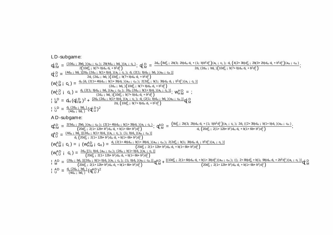
LD-subgame:
qLDHM = (10dH¡3bdL)(aH¡cH)¡2b(4dH¡bdL)(aL¡cL)
2(10d2H¡b(7+b)dHdL+b2d2
L); qLD
LM =2dH(8d2
H¡2b(3¡2b)dHdL+(1¡b)b2d2L)(aL¡cL)¡dL(4(2+3b)d2
H¡2b(3+2b)dHdL+b2d2L)(aH¡cH)
2dL(2dH¡bdL)(10d2H¡b(7+b)dHdL+b2d2
L);
qLDLU = (4dH¡bdL)[2dH(2dH¡b(1+b)dL)(aL¡cL)¡dL(2(1¡b)dH¡bdL)(aH¡cH)]
2dL(2dH¡bdL)(10d2H¡b(7+b)dHdL+b2d2
L)
(wLDLM¡cL) =
dH [dL(2(1+4b)dH¡b(1+3b)dL)(aH¡cH)¡2(2d2H¡b(1¡3b)dHdL¡b3d2
L)(aL¡cL)]
(2dH¡bdL)(10d2H¡b(7+b)dHdL+b2d2
L)
(wLDLU ¡ cL) = dL(2(1¡b)dH¡bdL)(aH¡cH)¡2dH(2dH¡b(1+b)dL)(aL¡cL)]
(2dH¡bdL)(10d2H
¡b(7+b)dHdL+b2d2L)
; wHDHM = ;
¦LDM = dH(qLD
HM)2 + [2dH(2dH¡b(1+b)dL)(aL¡cL)¡dL(2(1¡b)dH¡bdL)(aH¡cH)]
2dL(10d2H
¡b(7+b)dHdL+b2d2L)
qLDLM
¦LDU = dL(2dH¡bdL)
(4dH¡bdL)(qLD
LU )2
AD-subgame:
qADHM = 2(5dH¡2bdL)(aH¡cH)¡(2(1+4b)dH¡b(1+3b)dL)(aL¡cL)
(20d2H¡2(1+12b+b2)dHdL+b(1+6b+b2)d2
L); qAD
LM =(8d2
H¡2b(3¡2b)dHdL+(1¡b)b2d2L)(aL¡cL)¡2dL((2+3b)dH¡b(1+b)dL)(aH¡cH)
dL(20d2H¡2(1+12b+b2)dHdL+b(1+6b+b2)d2
L);
qADLU = (4dH¡bdL)[(2dH¡b(1+b)dL)(aL¡cL)¡(1¡b)dL)(aH¡cH)]
dL(20d2H
¡2(1+12b+b2)dHdL+b(1+6b+b2)d2L)
(wADLM¡cL) = ¡(wAD
HM¡cH) =dL(2(1+4b)dH¡b(1+3b)dL)(aH¡cH)¡2(2d2
H¡b(1¡3b)dHdL¡b3d2L)(aL¡cL)]
(20d2H¡2(1+12b+b2)dHdL+b(1+6b+b2)d2
L)
(wADLU ¡ cL) = 2dH [(1¡b)dL(aH¡cH)¡(2dH¡b(1+b)dL)(aL¡cL)]
(20d2H
¡2(1+12b+b2)dHdL+b(1+6b+b2)d2L)
¦ADM = (2dH¡bdL)[(2dH¡b(1+b)dL)(aL¡cL)¡(1¡b)dL)(aH¡cH)]
(20d2H¡2(1+12b+b2)dHdL+b(1+6b+b2)d2
L)qAD
LM+[(10d2
H¡2(1+6b)dHdL+b(1+3b)d2L)(aH¡cH)¡((¡2+8b)d2
H+b(1¡9b)dHdL+2b3d2L)(aL¡cL)]
(20d2H¡2(1+12b+b2)dHdL+b(1+6b+b2)d2
L)qLD
LM
¦ADU = dL(2dH¡bdL)
(4dH¡bdL)(qAD
LU )2
C Appendix: Proofs of Lemma 1 and Propo-
sitions 3 and 4.
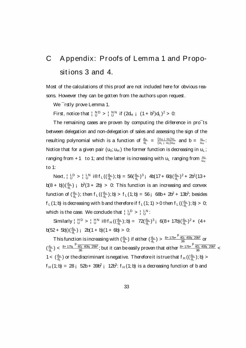
Most of the calculations of this proof are not included here for obvious rea-
sons. However they can be gotten from the authors upon request.
We ¯rstly prove Lemma 1.
First, notice that ¦NDU > ¦NN
U if (2dH ¡ (1 + b2)dL)2 > 0:
The remaining cases are proven by computing the di®erence in pro¯ts
between delegation and non-delegation of sales and assessing the sign of the
resulting polynomial which is a function of dH
dL= (uH¡u0)uL
(uL¡u0)uHand b = uL
uH:
Notice that for a given pair (u0; uH) the former function is decreasing in uL;
ranging from +1 to 1; and the latter is increasing with uL ranging from u0
uH
to 1:
Next, ¦LDU > ¦LN
U i® fL((dH
dL); b) = 56(dH
dL)3 ¡ 4b(17 + 6b)(dH
dL)2 + 2b2(13 +
b(8 + b))(dH
dL) ¡ b3(3 + 2b) > 0: This function is an increasing and convex
function of (dH
dL); then fL((dH
dL); b) > fL(1; b) = 56 ¡ 68b + 2b2 + 13b3; besides
fL(1; b) is decreasing with b and therefore if fL(1; 1) >0 then fL((dH
dL); b) > 0;
which is the case. We conclude that ¦LDU > ¦LN
U :
Similarly ¦HDU > ¦HN
U i® fH((dH
dL); b) = 72(dH
dL)3 ¡6(8+17b)(dH
dL)2 + (4+
b(52 + 5b))(dH
dL) ¡ 2b(1 + b)(1 + 6b) > 0:
This function is increasing with (dH
dL) if either (dH
dL) > 8+17b+
p40¡40b¡29b2
36or
(dH
dL) < 8+17b¡p
40¡40b¡29b2
36; but it can be easily proven that either 8+17b+
p40¡40b¡29b2
36<
1 < (dH
dL) or the discriminant is negative. Therefore it is true that fH((dH
dL); b) >
fH(1; b) = 28 ¡ 52b + 39b2 ¡ 12b3: fH(1; b) is a decreasing function of b and
33
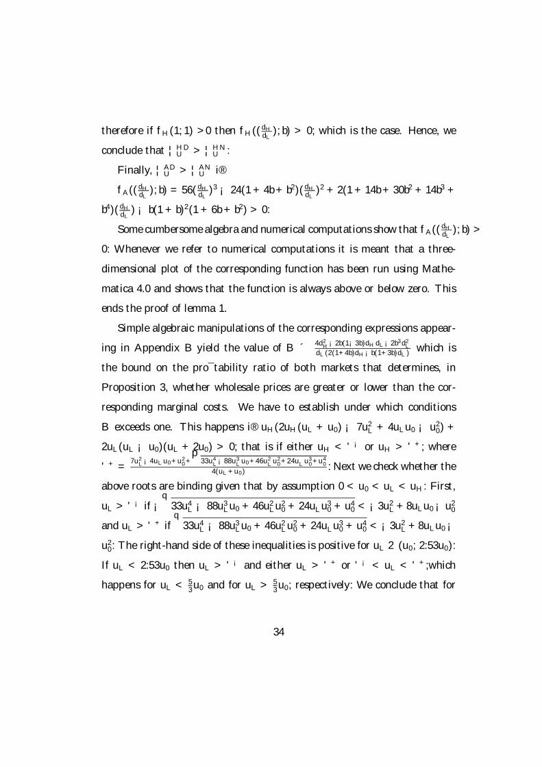
therefore if fH(1; 1) >0 then fH((dH
dL); b) > 0; which is the case. Hence, we
conclude that ¦HDU > ¦HN
U :
Finally, ¦ADU > ¦AN
U i®
fA((dH
dL); b) = 56(dH
dL)3 ¡ 24(1 + 4b + b2)(dH
dL)2 + 2(1 + 14b + 30b2 + 14b3 +
b4)(dH
dL) ¡ b(1 + b)2(1 + 6b + b2) > 0:
Some cumbersome algebra and numerical computations show that fA((dH
dL); b) >
0: Whenever we refer to numerical computations it is meant that a three-
dimensional plot of the corresponding function has been run using Mathe-
matica 4.0 and shows that the function is always above or below zero. This
ends the proof of lemma 1.
Simple algebraic manipulations of the corresponding expressions appear-
ing in Appendix B yield the value of B ´ 4d2H¡2b(1¡3b)dHdL¡2b3d2
L
dL(2(1+4b)dH¡b(1+3b)dL)which is
the bound on the pro¯tability ratio of both markets that determines, in
Proposition 3, whether wholesale prices are greater or lower than the cor-
responding marginal costs. We have to establish under which conditions
B exceeds one. This happens i® uH(2uH(uL + u0) ¡ 7u2L + 4uLu0 ¡ u2
0) +
2uL(uL ¡ u0)(uL + 2u0) > 0; that is if either uH < '¡ or uH > '+; where
'+ =7u2
L¡4uLu0+u20+
p33u4
L¡88u3
Lu0+46u2
Lu2
0+24uL
u30+u4
0
4(uL+u0): Next we check whether the
above roots are binding given that by assumption 0 < u0 < uL < uH : First,
uL > '¡ if ¡q
33u4L ¡ 88u3
Lu0 + 46u2Lu2
0 + 24uLu30 + u4
0 < ¡3u2L +8uLu0 ¡u2
0
and uL > '+ ifq
33u4L ¡ 88u3
Lu0 + 46u2Lu2
0 + 24uLu30 + u4
0 < ¡3u2L +8uLu0 ¡
u20: The right-hand side of these inequalities is positive for uL 2 (u0; 2:53u0):
If uL < 2:53u0 then uL > '¡ and either uL > '+ or '¡ < uL < '+;which
happens for uL < 53u0 and for uL > 5
3u0; respectively: We conclude that for
34
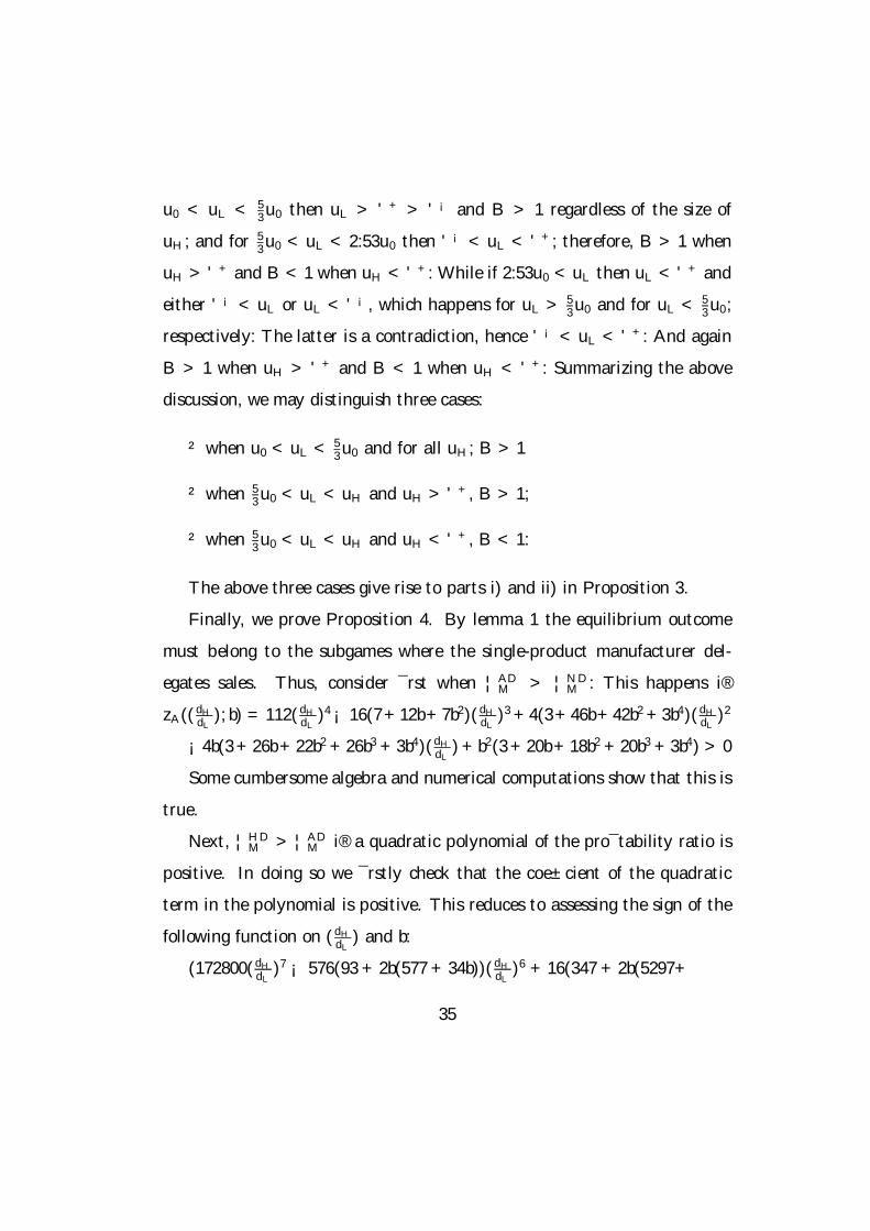
u0 < uL < 53u0 then uL > '+ > '¡ and B > 1 regardless of the size of
uH ; and for 53u0 < uL < 2:53u0 then '¡ < uL < '+; therefore, B > 1 when
uH > '+ and B < 1 when uH < '+: While if 2:53u0 < uL then uL < '+ and
either '¡ < uL or uL < '¡, which happens for uL > 53u0 and for uL < 5
3u0;
respectively: The latter is a contradiction, hence '¡ < uL < '+: And again
B > 1 when uH > '+ and B < 1 when uH < '+: Summarizing the above
discussion, we may distinguish three cases:
² when u0 < uL < 53u0 and for all uH ; B > 1
² when 53u0 < uL < uH and uH > '+, B > 1;
² when 53u0 < uL < uH and uH < '+, B < 1:
The above three cases give rise to parts i) and ii) in Proposition 3.
Finally, we prove Proposition 4. By lemma 1 the equilibrium outcome
must belong to the subgames where the single-product manufacturer del-
egates sales. Thus, consider ¯rst when ¦ADM > ¦ND
M : This happens i®
zA((dH
dL); b) = 112(dH
dL)4 ¡16(7+12b+7b2)(dH
dL)3 +4(3+46b+42b2 +3b4)(dH
dL)2
¡4b(3 + 26b + 22b2 + 26b3 + 3b4)(dH
dL) + b2(3 + 20b + 18b2 + 20b3 + 3b4) > 0
Some cumbersome algebra and numerical computations show that this is
true.
Next, ¦HDM > ¦AD
M i® a quadratic polynomial of the pro¯tability ratio is
positive. In doing so we ¯rstly check that the coe±cient of the quadratic
term in the polynomial is positive. This reduces to assessing the sign of the
following function on (dH
dL) and b:
(172800(dH
dL)7 ¡ 576(93 + 2b(577 + 34b))(dH
dL)6 + 16(347 + 2b(5297+
35
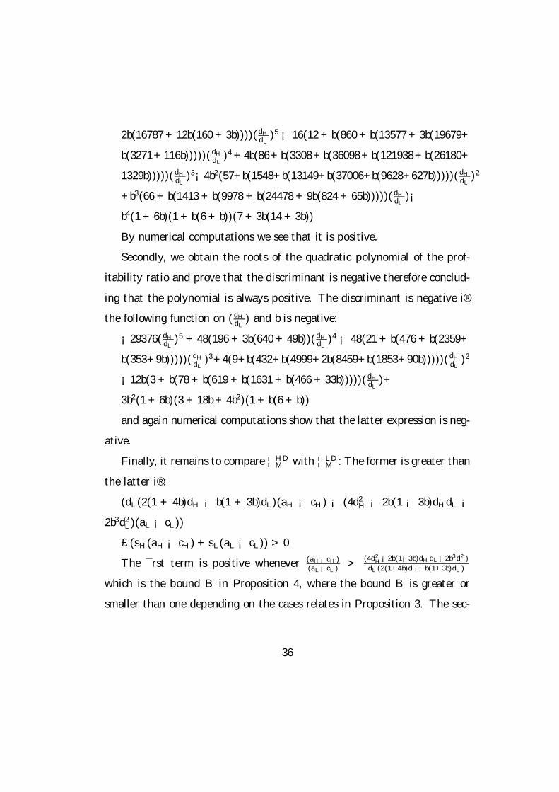
2b(16787 + 12b(160 + 3b))))(dH
dL)5 ¡ 16(12 + b(860 + b(13577 + 3b(19679+
b(3271+116b)))))(dH
dL)4 +4b(86+ b(3308+ b(36098+ b(121938+ b(26180+
1329b)))))(dH
dL)3¡4b2(57+b(1548+b(13149+b(37006+b(9628+627b)))))(dH
dL)2
+b3(66 + b(1413 + b(9978 + b(24478 + 9b(824 + 65b)))))(dH
dL)¡
b4(1 + 6b)(1 + b(6 + b))(7 + 3b(14 + 3b))
By numerical computations we see that it is positive.
Secondly, we obtain the roots of the quadratic polynomial of the prof-
itability ratio and prove that the discriminant is negative therefore conclud-
ing that the polynomial is always positive. The discriminant is negative i®
the following function on (dH
dL) and b is negative:
¡29376(dH
dL)5 + 48(196 + 3b(640 + 49b))(dH
dL)4 ¡ 48(21 + b(476 + b(2359+
b(353+9b)))))(dH
dL)3+4(9+b(432+b(4999+2b(8459+b(1853+90b)))))(dH
dL)2
¡12b(3 + b(78 + b(619 + b(1631 + b(466 + 33b)))))(dH
dL)+
3b2(1 + 6b)(3 + 18b + 4b2)(1 + b(6 + b))
and again numerical computations show that the latter expression is neg-
ative.
Finally, it remains to compare ¦HDM with ¦LD
M : The former is greater than
the latter i®:
(dL(2(1 + 4b)dH ¡ b(1 + 3b)dL)(aH ¡ cH) ¡ (4d2H ¡ 2b(1 ¡ 3b)dHdL ¡
2b3d2L)(aL ¡ cL))
£(sH(aH ¡ cH) + sL(aL ¡ cL)) > 0
The ¯rst term is positive whenever (aH¡cH)(aL¡cL)
>(4d2
H¡2b(1¡3b)dHdL¡2b3d2L)
dL(2(1+4b)dH¡b(1+3b)dL)
which is the bound B in Proposition 4, where the bound B is greater or
smaller than one depending on the cases relates in Proposition 3. The sec-
36
ond is positive i® (aH¡cH)(aL¡cL)
< sL
¡sH; where sL > 0 and sH < 0: Algebraic
together with numerical computations show that sL
¡sHis greater than the up-
perbound on the pro¯tability ratio which ensures positive outputs, and then,
this second term is always positive. The result of Proposition 4 follows.
37
MH \\ ML action N action D
action N LH
LLHHNNH bdd
cabcaq
−−−−
=4
)()(2
LLH
HHLLLHNNL dbdd
cadcadq
)4(
)()(2
−−−−
=
HLH
LLHHHLHNDH dbdd
cabdcabddq
)2(4
)(2))(4(
−−−−−
=
LLH
HHLLLHNDL dbdd
cadcadq
)2(2
)()(2
−−−−
=
action D )2(2
)()(2
LH
LLHHDNH bdd
cabcaq
−−−−
=
LLH
HHLLLLHDNL dbdd
cadcabddq
)2(4
)(2))(4(
−−−−−
=
( ))1216(
)(2))(4(2222LLHH
LLHHHLHDDH dbdbdd
cabdcabddq
+−−−−−
=
( )LLLHH
HHLLLLHHDDL ddbdbdd
cadcabdddq
)1216(
)(2))(4(2222 +−
−−−−=
TABLE 1A. Equilibrium quantities of game G1.
MH \\ ML action N action D
action N
( )2
2
)4(
)()(2
LH
LLHHHNNH bdd
cabcad
−−−−=Π
( )2
2
)4(
)()(2
LHL
HHLLLHNNL bddd
cadcad
−−−−=Π
( )2
2
)2(16
)(2))(4(
LHH
LLHHHLHNDH bddd
cabdcabdd
−−−−−=Π
( ))2(8
)()(2 2
LHLH
HHLLLHNDL bdddd
cadcad
−−−−=Π
action D
( ))2(8
)()(2 2
LH
LLHHDNH bdd
cabca
−−−−
=Π
( )2
2
)2(16
)(2))(4(
LHL
HHLLLLHDNL bddd
cadcabdd
−−−−−
=Π
( )2222
2
)1216(
)(2))(4()2(2
LLHH
LLHHHLHLHDDH dbdbdd
cabdcabddbdd
+−−−−−−
=Π
( )2222
2
)1216(
)(2))(4()2(2
LLHHL
HHLLLLHLHHDDL dbdbddd
cadcabddbddd
+−−−−−−
=Π
TABLE 1B. Payoffs of game G1. Delegation in a vertically differentiated duopoly.
M1 \\ M2 action N action D
action N L
LLNN
d
caq
31
−=
L
LLNN
d
caq
32
−=
LLH
HHLLLLHND
dbdd
cadcabddq
)2(4
)(2))(4(1 −
−−−−=
)2(2
)()(22
LH
LLHHND
bdd
cabcaq
−−−−
=
action D )2(2
)()(21
LH
LLHHDN
bdd
cabcaq
−−−−
=
LLH
HHLLLLHDN
dbdd
cadcabddq
)2(4
)(2))(4(2 −
−−−−=
H
HHDD
d
caq
5
)(21
−=
H
HHDD
d
caq
5
)(22
−=
TABLE 2A. Equilibrium quantities of game G2.
M1 \\ M2 action N action D
action N L
LLNN
d
ca
9
)( 2
1
−=Π
L
LLNN
d
ca
9
)( 2
2
−=Π
( )LLH
HHLLLLHND
dbdd
cadcabdd2
2
1)2(16
)(2))(4(
−−−−−
=Π
( ))2(8
)()(2 2
2LH
LLHHND
bdd
cabca
−−−−
=Π
action D
( ))2(8
)()(2 2
1LH
LLHHDN
bdd
cabca
−−−−
=Π
( )LLH
HHLLLLHDN
dbdd
cadcabdd2
2
2)2(16
)(2))(4(
−−−−−=Π
H
HHDD
d
ca
25
)(2 2
1
−=Π
H
HHDD
d
ca
25
)(2 2
2
−=Π
TABLE 2B. Payoffs of game G2. Endogeneous selection of quality by delegation.
References
[1] Bernheim, B. and M. Whinston (1998), "Exclusive Dealing", Jour-
nal of Political Economy, 106, 64-103.
[2] Besanko, D. and M.K. Perry (1993), "Equilibrium Incentives for
Exclusive Dealing in a Di®erentiated Products Oligopoly", Rand Journal
of Economics, 24, 646-667.
[3] Besanko, D. and M.K. Perry (1994), "Exclusive Dealing in a Spa-
tial Model of Retail Competition", International Journal of Industrial
Organization, 12, 297-329.
[4] Bonanno, G. and J. Vickers (1988), "Vertical Separation", Journal
of Industrial Economics, 36, 257-265.
[5] Chang, M-H. (1992), "Exclusive Dealing Contracts in a Successive
Duopoly with Side Payments", Southern Economic Journal, October,
180-193.
[6] Dobson, P.W. and M. Waterson (1996), "Product Range and In-
ter¯rm Competition", Journal of Economics and Management Strategy,
5, 317-341.
[7] Dobson, P.W. and M. Waterson (1997), "Exclusive Trading Con-
tracts in Successive Di®erentiated Duopoly", Southern Economic Jour-
nal, 361-377.
42
[8] Gabrielsen, T.S. (1996), "The Foreclosure Argument for Exclusive
Dealing: The Case of Di®erentiated Retailers", Journal of Economics,
63, 25-40.
[9] Gabrielsen, T.S. (1997), "Equilibrium Retail Distribution Systems",
International Journal of Industrial Organization, 16, 105-120.
[10] Gabrielsen, T.S. and L. S¿rgard (1999), "Exclusive versus Com-
mon Dealership", Southern Economic Journal, 66, 353-366.
[11] Gabszewicz, J.J. and J.F. Thisse (1979), "Price Competition,
Quality and Income Disparities", Journal of Economic Theory, 20, 340-
354.
[12] Hoch, S.J. and S. Banerji (1993), "When do private labels suc-
ceed?", Sloan Management Review, 34, 57-67.
[13] Irmen, A. (1998), "Precommitment in Competing Vertical Chains",
Journal of Economic Surveys, 12, 333-359.
[14] Lin, Y.J. (1990), "The Dampening-of-Competition E®ect of Exclusive
Dealing", Journal of Industrial Economics, 39, 209-223.
[15] O'Brien, D. and G. Sha®er (1993), "On the Dampening-of-
Competition E®ect of Exclusive Dealing", Journal of Industrial Eco-
nomics, 41, 215-221.
[16] O'Brien, D. and G. Sha®er (1997), "Nonlinear Supply Contracts,
Exclusive Dealing, and Equilibrium Market Foreclosure", Journal of
Economics and Management Strategy, 6, 755-785.
43
[17] Moner-Colonques, R., J.J. Sempere-Monerris and A. Urbano
(1999), "Equilibrium Distribution Systems under Retailers' Strategic
Behaviour", mimeo University of Valencia.
[18] Narasimhan, C. and R. Wilcox (1998), "Private Labels and the
Channel Relationship: A Cross-Category Analysis", Journal of Busi-
ness, 71, 573-600.
[19] Rey, P. and J. Stiglitz (1995), "The Role of Exclusive Territories in
Producers' Competition", Rand Journal of Economics, 26, 431-451.
[20] Vickers, J. (1985), "Delegation and the Theory of the Firm", Eco-
nomic Journal, Conference Supplement, 138-147.
44
Recommended