1
Prof. David R. JacksonECE Dept.
Spring 2014
Notes 36
ECE 6341

2
Radiation Physics in Layered Media
Note: TMz and also TEy (since )0z
00 0
0
11
4y x
z
jk y jk xTEx x
y
A
Ik e e dk
j k
For y > 0:
ˆ ,zE z E x y
y
0Ix
rh
Line source on grounded substrate

3
Reflection Coefficient
0
0
TE TEin x xTE
x TE TEin x x
Z k Z kk
Z k Z k
1 1tanTE TEin x yZ k jZ k h
01
1
TE
y
Zk
1/ 22 2
1 1y xk k k
where
00
0
TE
y
Zk
1/ 22 2
0 0y xk k k
00TEZ
01TEZ
I V+ -
z

4
Poles
Poles:
0
0
TE TEin x xTE
x TE TEin x x
Z k Z kk
Z k Z k
0TE TEin xp xpZ k Z k
This is the same equation as the TRE for finding the wavenumber of a surface wave:
kxp = roots of TRE = kxSW
x xpk k
0TE SW TE SWin x xZ k Z k 00
TEZ
01TEZ
I V+ -
z
5
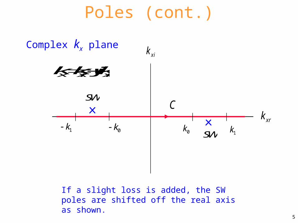
If a slight loss is added, the SW poles are shifted off the real axis as shown.
Poles (cont.)
Complex kx plane
Cxrk
xik
SW0k1k0k1k
SW
x xr xik k jk

6
Poles (cont.)
C
xrk
xik
0k1k
0k1k
For the lossless case, two possible paths are shown here.
C
xrk
xik
0k1k
0k1k

7
Review of Branch Cuts and Branch Points
In the next few slides we review the basic concepts of branch points and branch cuts.

8
Consider 1/ 2f z z jz r e
1/21/2 /2j jz r e r e
1z 0 : 1/2 1z
2 : 1/2 1z
4 : 1/2 1z
There are two possible values.
Choose
Branch Cuts and Points (cont.)

9
The concept is illustrated for 1/ 2f z z jz r e
1/ 2 / 2jz r e
x
y
AB C
r = 1
Consider what happens if we encircle the origin:
Branch Cuts and Points (cont.)
10
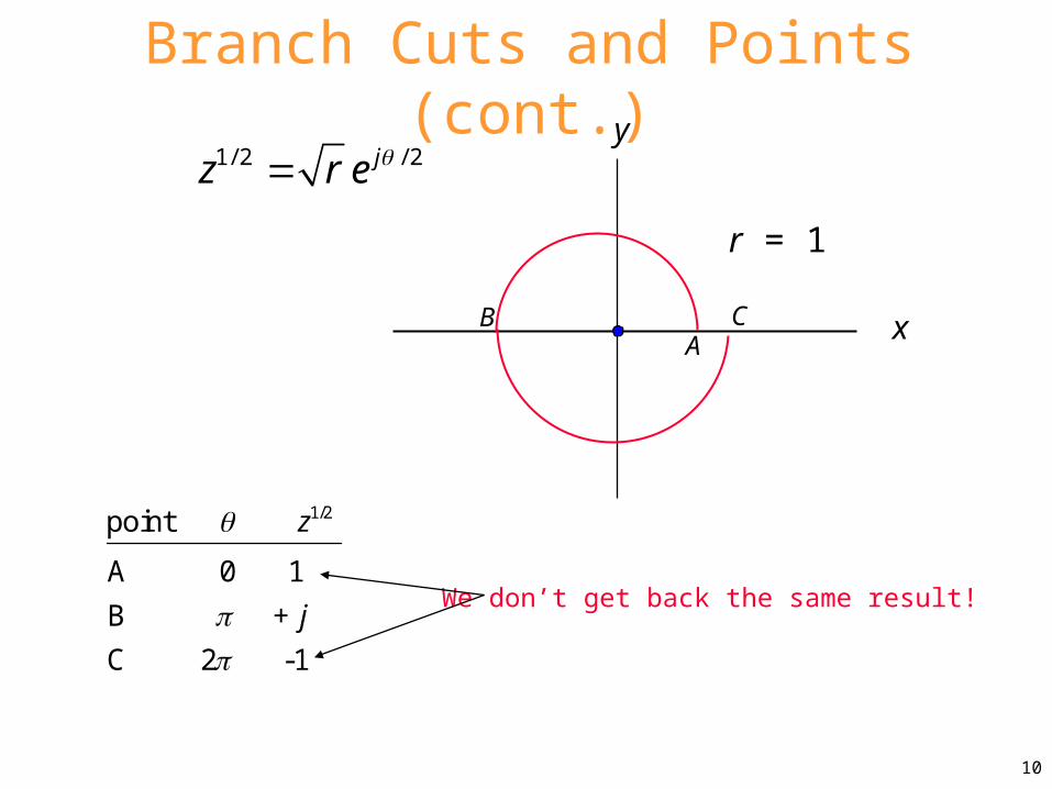
Branch Cuts and Points (cont.)
1/ 2 / 2jz r e
1/2
A 0 1
B +
C 2 -1
z
j
point
We don’t get back the same result!
x
y
AB C
r = 1
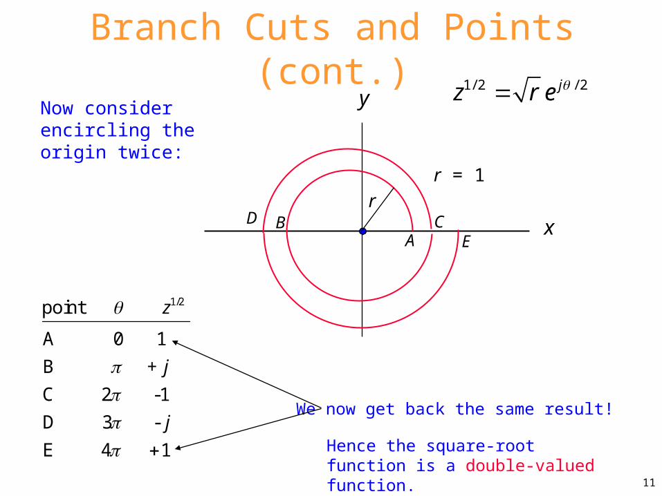
11
Now consider encircling the origin twice:
1/ 2 / 2jz r e
1/2
A 0 1
B +
C 2 -1
D 3 -
E 4 1
z
j
j
point
We now get back the same result!
Hence the square-root function is a double-valued function.
Branch Cuts and Points (cont.)
x
y
AB CD
E
r = 1
r

12
In order to make the square-root function single-valued, we must put a “barrier” or “branch cut”.
The origin is called a branch point: we are not allowed to encircle it if we wish to make the square-root function single-valued.
x
Branch cut
y
Here the branch cut was chosen to lie on the negative real axis (an arbitrary choice)
Branch Cuts and Points (cont.)

13
We must now choose what “branch” of the function we want.
jz r e 1/ 2 / 2jz r e
x
Branch cut
y
1z 1/ 2 1z
Branch Cuts and Points (cont.)
This is the "principle" branch, denoted by z
MATLAB :
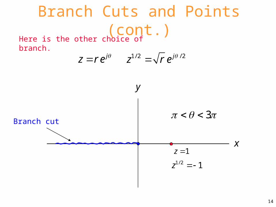
14
Here is the other choice of branch.
jz r e 1/ 2 / 2jz r e
x
Branch cut
y
3
1z 1/ 2 1z
Branch Cuts and Points (cont.)

15
Note that the function is discontinuous across the branch cut.
jz r e 1/ 2 / 2jz r e
x
Branch cut
y
1z 1/2 1z
1,z
1,z
1/ 2z j
1/ 2z j
Branch Cuts and Points (cont.)
16
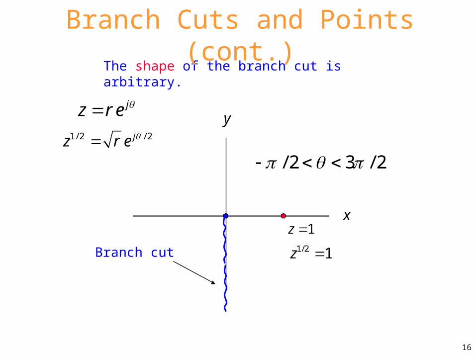
The shape of the branch cut is arbitrary.
jz r e 1/ 2 / 2jz r e
x
Branch cut
y
/ 2 3 / 2
1z 1/2 1z
Branch Cuts and Points (cont.)

17
The branch cut does not even have to be a straight line
jz r e 1/ 2 / 2jz r e
In this case the branch is determined by requiring that the square-root function (and hence the angle ) change continuously as we start from a specified value (e.g., z = 1).
x
Branch cut
y
1z 1/2 1z
1z 1/ 2z j
z j 1/ 2 / 4 1 / 2jz e j
z j
1/ 2 / 4 1 / 2jz e j
Branch Cuts and Points (cont.)

18
Consider this function:
1/ 22( ) 1f z z
Branch Cuts and Points (cont.)
What do the branch points and branch cuts look like for this function?
(similar to our wavenumber function)

19
1/ 2 1/ 21/ 2 1/ 2 1/ 22( ) 1 1 1 1 1f z z z z z z
Branch Cuts and Points (cont.)
x
y
1
1
There are two branch cuts: we are not allowed to encircle either branch point.

20
1/ 21/ 2 1/ 2 1/ 21 2( ) 1 1f z z z w w
Branch Cuts and Points (cont.)
Geometric interpretation
x
y
1
11w
2w
12
1 2/ 2 / 21 2( ) j jf z r e r e
1
2
1 1
2 2
1
( 1)
j
j
w z r e
w z r e
The function f (z) is unique once we specify its value at any point. (The function must change continuously away from this point.)

21
Riemann Surface
Georg Friedrich Bernhard Riemann (September 17, 1826 – July 20, 1866) was an influential German mathematician who made lasting contributions to analysis and differential geometry, some of them enabling the later development of general relativity.
The function z1/2 is continuous everywhere on this surface (there are no branch cuts). It also assumes all possible values on the surface.
The Riemann surface is really multiple complex planes connected together.
The function z1/2 has a surface with two sheets.
22
Riemann Surface
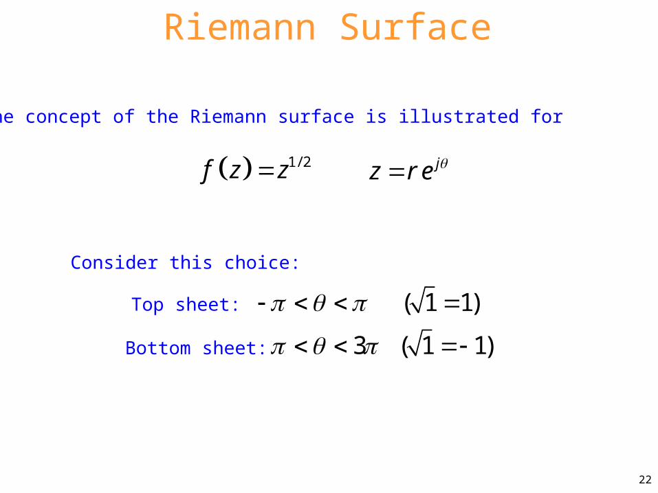
The concept of the Riemann surface is illustrated for
1/ 2f z z
( 1 1)
3 ( 1 1)
Top sheet:
Bottom sheet:
Consider this choice:
jz r e

23
Riemann Surface (cont.)x
y
BD
Top
Bottom
BD
D
B
B
Dside view
x
y
top view
24
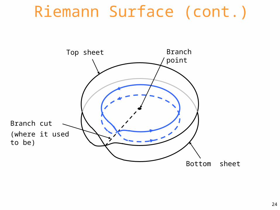
Riemann Surface (cont.)
Bottom sheet
Top sheet
Branch cut
(where it used to be)
Branch point
25
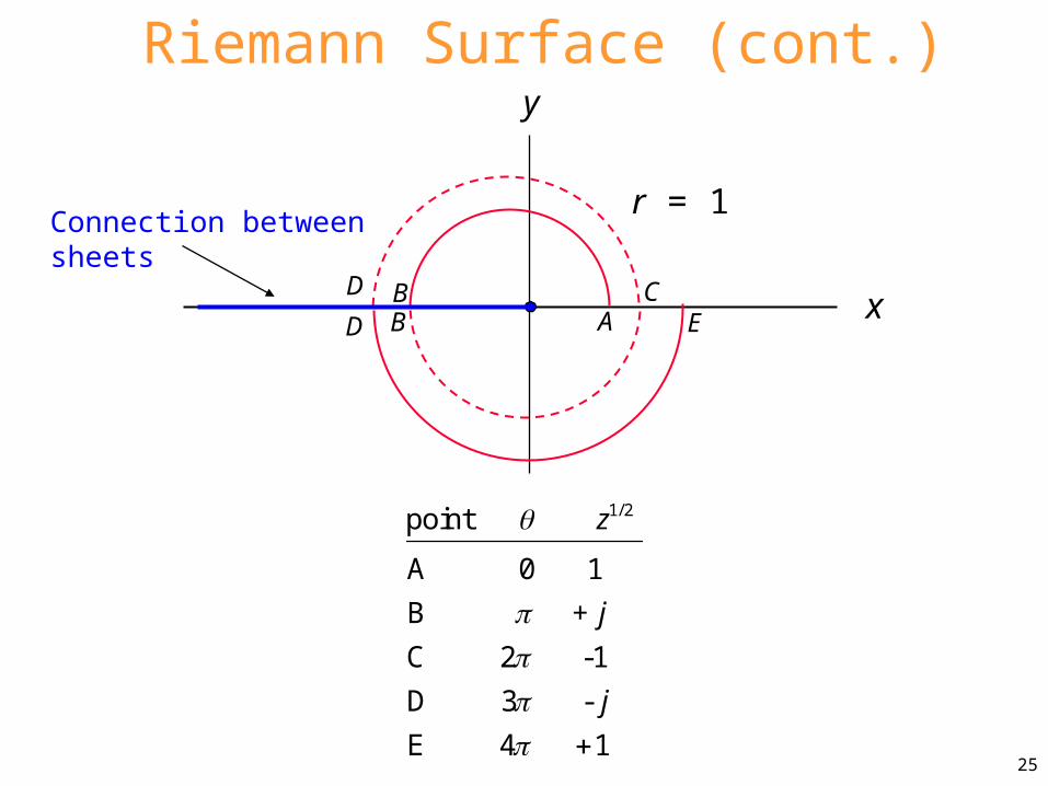
Riemann Surface (cont.)
x
y
AB CD
EBD
Connection betweensheets
1/2
A 0 1
B +
C 2 -1
D 3 -
E 4 1
z
j
j
point
r = 1

26
Branch Cuts in Radiation Problem
Now we return to the original problem:
1
2 2 20 0y xk k k
00 0
0
11
4y x
z
jk y jk xTEx x
y
A
Ik e e dk
j k
Note: There are no branch points from ky1:
1
2 2 21 1y xk k k 1 1tanTE TE
in x yZ k jZ k h 01
1
TE
y
Zk
27
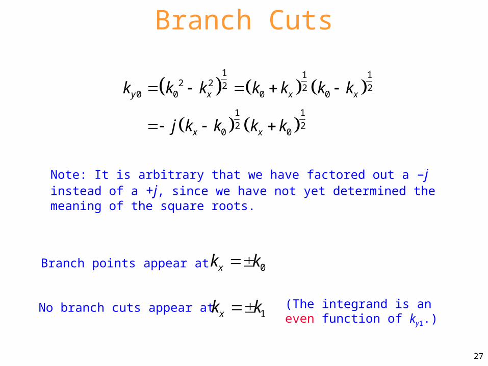
Branch Cuts
1 1 12 2 2 2 2
0 0 0 0
1 1
2 20 0
y x x x
x x
k k k k k k k
j k k k k
Branch points appear at 0xk k
No branch cuts appear at 1xk k (The integrand is an even function of ky1.)
Note: It is arbitrary that we have factored out a –j instead of a +j, since we have not yet determined the meaning of the square roots.

28
Branch Cuts (cont.)
1 1
2 20 0 0y x xk j k k k k
Cxrk
xik
0k
0k
1k1k
Branch cuts are lines we are not allowed to cross.

29
For 0
0 0
,x
y y
k k
k j k
real
xrk
xik
0k
0k
Choose
0
0
arg 0
arg 0
x
x
k k
k k
This choice then uniquely defines ky0
everywhere in the complex plane.
1/22 20 0y xk k k
1 1
2 20 0 0y x xk j k k k k
Branch Cuts (cont.)
at this point
0 0y yk j k

30
For
0
,
0x
x
k
k k
real we have
0
0
arg
arg 0
x
x
k k
k k
/ 20 0 0
jy x xk j k k e k k
0 0y yk k
Hence
Branch Cuts (cont.)
xik
xrk0k 0k
31
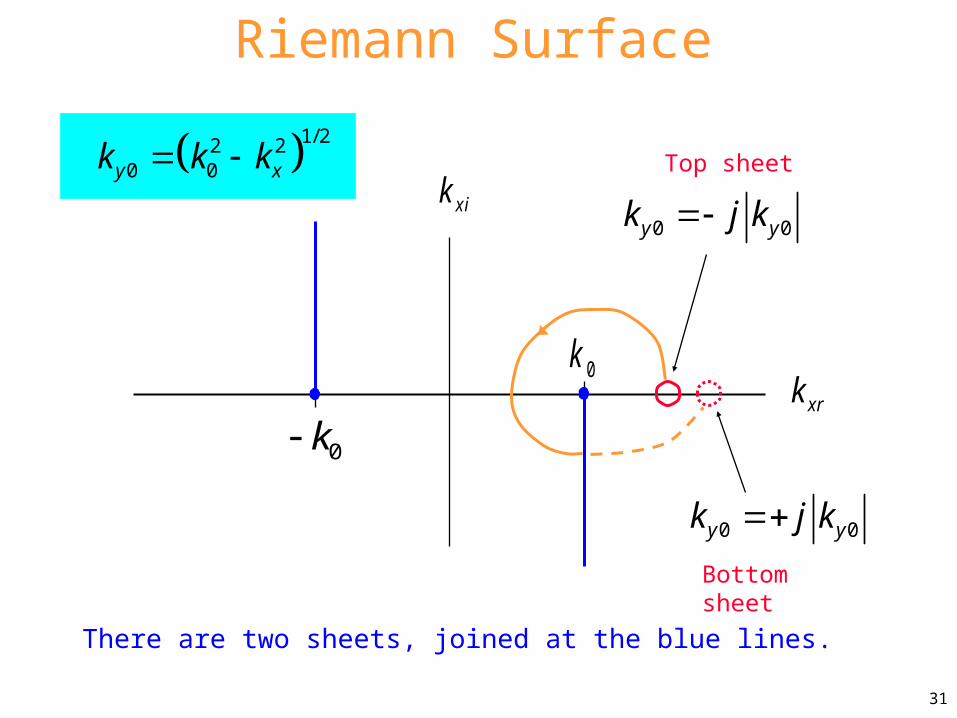
Riemann Surface
1/22 20 0y xk k k
There are two sheets, joined at the blue lines.
xik
xrk
0k
0k
Top sheet
Bottom sheet
0 0y yk j k
0 0y yk j k

32
Proper / Improper Regions
Let
“Proper” region:
0 0 0
x xr xik k jk
k k jk
1
2 2 20 0y xk k k
“Improper” region:
0
0
Im 0
Im 0
y
y
k
k
Boundary: 0Im 0yk
2 2 20 0 real >0y xk k k
The goal is to figure out which regions of the complex plane are "proper" and "improper."

33
Proper / Improper Regions (cont.)
Hence
One point on curve:
2 2 2 20 0 0 02 2 real 0xr xi xr xik k k k j k k k k
0 0xr xik k k k
0
0
xr
xi
k k
k k
xik
0k
0 k
xrk
2
2
0 0 real 0xr xik jk k jk
Therefore
0 0 0xk k k jk
(hyperbolas)
0 0 0k k jk
34
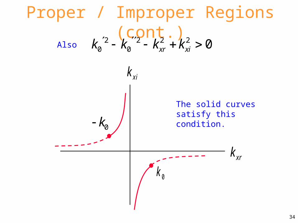
Proper / Improper Regions (cont.)
Also2 2 2 2
0 0 0xr xik k k k
xik
0k
0 k
xrk
The solid curves satisfy this condition.
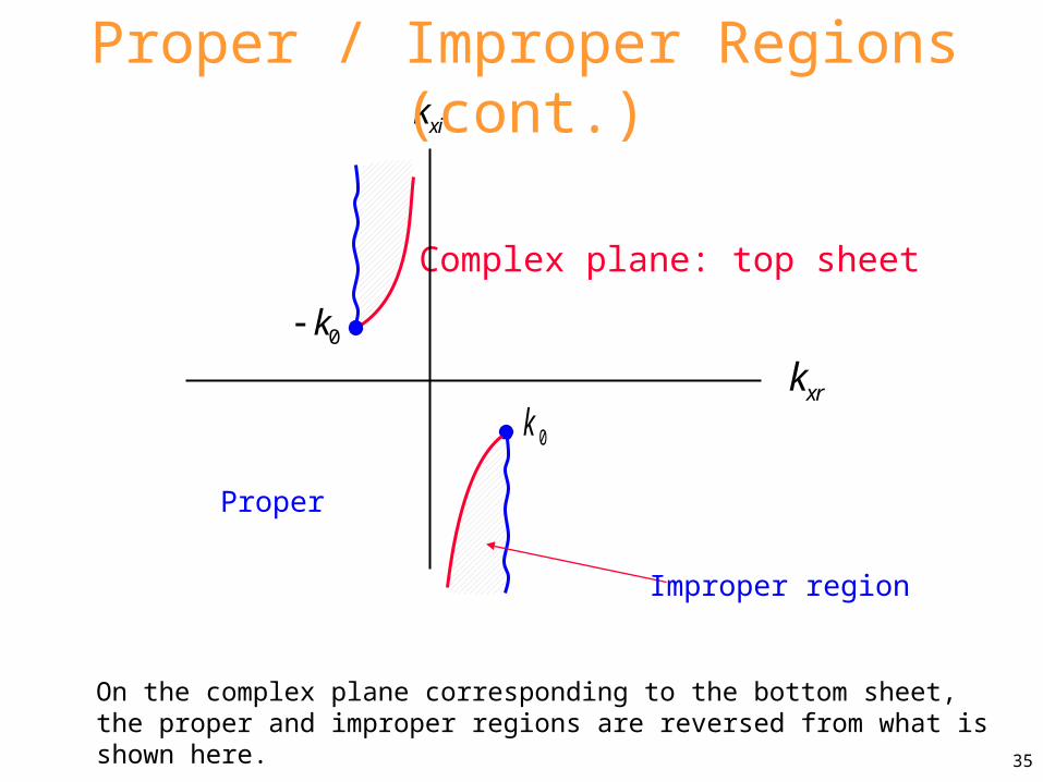
35
Complex plane: top sheet
xik
0k
0 k
xrk
Improper region
Proper
On the complex plane corresponding to the bottom sheet, the proper and improper regions are reversed from what is shown here.
Proper / Improper Regions (cont.)

36
Sommerfeld Branch Cuts
Complex plane corresponding to top sheet: proper everywhereComplex plane corresponding to bottom sheet: improper everywhere
xik
0k
0 k
xrk
Hyperbola

37
Sommerfeld Branch Cuts
Note: We can think of a single complex plane with branch cuts, or a Riemann surface with hyperbolic-shaped “ramps” connecting the two sheets.
xik
0k
0 k
xrk
Riemann surface
xik
0k
0 k
xrk
Complex plane
The Riemann surface allows us to show all possible poles, both proper (surface-wave) and improper (leaky-wave).
38
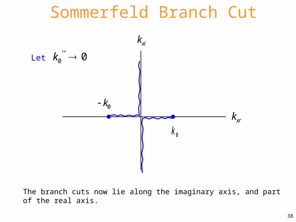
Sommerfeld Branch Cut
Let
xik
0k
0 k
xrk
0 0k
The branch cuts now lie along the imaginary axis, and part of the real axis.
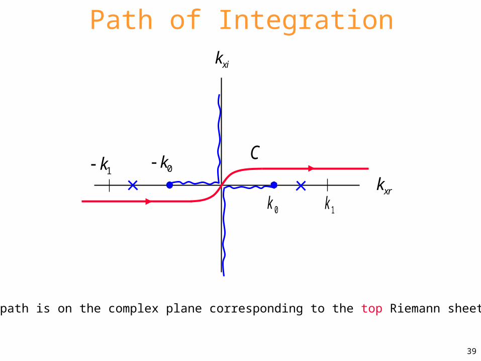
39
Path of Integration
xik
0k
0 k
xrk
1k
1 kC
The path is on the complex plane corresponding to the top Riemann sheet.

40
Numerical Path of Integration
xik
0k
0 k
xrk1k
1 k
C
41
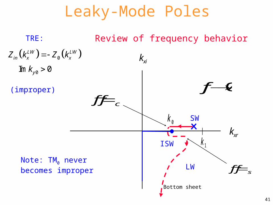
Leaky-Mode Poles
(improper)
0
0Im 0
LW LWin x x
y
Z k Z k
k
Note: TM0 never becomes improper
Review of frequency behavior
xik
0k
xrk1k
cf f
SW
ISW
LW
0f
sf f
TRE:
Bottom sheet

42
Riemann Surface
xik
0k
0 k
xrk1k
1 kC
SWPLWP
BP
0 0Re LWxpk k k
The LW pole is then “close” to the path on the Riemann surface (and it usually makes an important contribution).
We can now show the leaky-wave poles!
LW LW LWxpk j
ReLW LWxpk

43
SW and CS Fields
Total field = surface-wave (SW) field + continuous-spectrum (CS) field
xik
0k
xrk1k
SWLW
bC
CS fieldSW field
pC
Note: The CS field indirectly accounts for the LW pole.
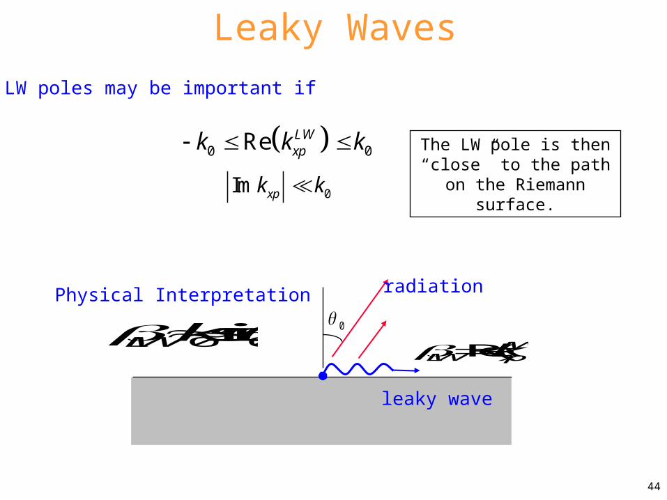
44
Leaky Waves
LW poles may be important if
0 0Re LWxpk k k
0Im xpk k
Physical Interpretation
Re( )LWLW xpk
0
leaky wave
radiation
0 0sinLW k
The LW pole is then “close” to the path on the
Riemann surface.

45
Improper Nature of LWs
The rays are stronger near the beginning of the wave: this gives us exponential growth vertically.
Region of strong leakage fields
LWxpk j
“leakage rays”
46
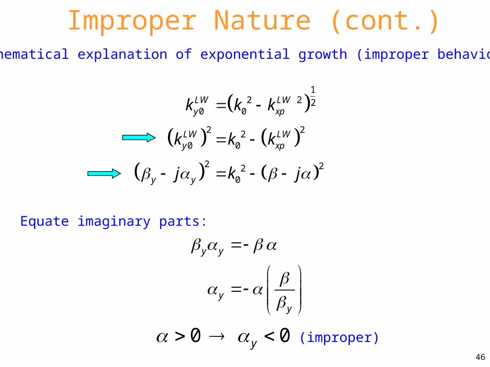
Improper Nature (cont.)Mathematical explanation of exponential growth (improper behavior):
Equate imaginary parts:
12 2 2
0 0
2 220 0
2 220
LW LWy xp
LW LWy xp
y y
k k k
k k k
j k j
y y
yy
(improper)0 0y
Recommended