1
Protected area effectiveness in European Russia: A post-matching panel data analysis
Kelly J. Wendland
Department of Conservation Social Sciences
University of Idaho
Moscow, ID, 83843, USA
Matthias Baumann
Department of Forest and Wildlife Ecology
University of Wisconsin-Madison
Madison, WI, USA
David J. Lewis
Department of Applied Economics
Oregon State University
Corvallis, OR, USA
Anika Sieber
Geography Department
Humboldt-University Berlin
Berlin, Germany
Volker C. Radeloff

2
Department of Forest and Wildlife Ecology
University of Wisconsin-Madison
Madison, WI, USA
The authors are, respectively, assistant professor, Department of Conservation Social Sciences,
University of Idaho; Ph.D. candidate, Department of Forest and Wildlife Ecology, University of
Wisconsin-Madison; associate professor, Department of Applied Economics, Oregon State
University; Ph.D. candidate, Geography Department, Humboldt-University Berlin; professor,
Department of Forest and Wildlife Ecology, University of Wisconsin-Madison. Please send
inquiries to [email protected].
The authors gratefully acknowledge support from NASA’s Land-Cover and Land-Use Change
Program (Project Number: NNX08AK776), the German Science Foundation (DFG) (LUCC-BIO
Project, Number: 32103109) and the Einstein Foundation Berlin. This paper was greatly
improved by the comments of two anonymous reviewers and J. Alix-Garcia; all remaining errors
are our own.
3
ABSTRACT
We estimate the impact of strict and multiple use protected areas on forest disturbance in
European Russia between 1985 and 2010. We construct a spatial panel dataset from remote
sensing that includes five periods of change. We match protected areas to areas outside of
protection and compare coefficients from fixed versus random effect panel regressions. We find
that strict protected areas had small but significantly significant impacts on disturbance; multiple
use areas had few statistically significant impacts on disturbance. Random effects underestimate
park effectiveness compared to fixed effects, serving as a cautionary note for evaluations where
time-invariant unobservables are important.
Keywords: Russia; forest disturbance; program evaluation; logging; matching; protected areas
4
I. INTRODUCTION
Protected areas are a cornerstone for biodiversity conservation and the provision of
ecosystem services such as carbon sequestration (Rodrigues et al. 2004; Scharlemann et al.
2010). They cover about 13% of terrestrial land, with continuing efforts to increase this area
(Brooks et al. 2004; Jenkins and Joppa 2009). However, protected areas face many threats in
conserving biodiversity and provisioning ecosystem services: they are often inadequately funded
and staffed (Bruner et al. 2001), and are increasingly called on to meet multiple social objectives
(Dudley et al. 1999; Naughton-Treves, Holland and Brandon 2005; Sims 2010; Ferraro and
Hanauer 2011). Furthermore, it is not always clear how much of an effect protected areas have,
even in limiting forest loss, because where protected areas are placed strongly affects the
additional benefits they bring to protecting biodiversity and ecosystem services (Joppa and Pfaff
2010). The majority of studies that examine protected area effectiveness have focused on the
tropics though, in particular Costa Rica and Brazil (e.g., Andam et al. 2008; Pfaff et al. 2009;
Ferraro and Hanauer 2011; Nelson and Chomitz 2012; Nolte et al. 2013; Pfaff et al. 2013), and
little is known about how effective protected areas are during times of rapid socioeconomic
changes.
This paper’s first objective is to estimate how effective different types of protected areas
were at limiting forest disturbance in post-Soviet European Russia. The collapse of the Soviet
Union in 1991 was one of the most dramatic political and socioeconomic changes in recent
history, leading to rapid and unprecedented land use changes, including agricultural
abandonment, decreased commercial logging, and increased illegal logging (Eikeland,
Eythorsson and Ivanova 2004; Torniainen, Saastamoinen and Petrov 2006; Prishchepov et al.
2012). During this period, forest management responsibilities in Russia changed several times,
5
leading to confusion over management responsibilities (Sobolev et al. 1995; Colwell et al. 1997;
Pryde 1997; Ostergren and Jacques 2002). There were also rapid decreases in budgets for
biodiversity protection: one estimate puts post-transition budgets at about 10% of their 1989
levels (Wells and Williams 1998). During this same period, the number of protected areas
expanded rapidly in Russia (Radeloff et al. 2013), and there are continued calls to increase the
protected area network (Krever, Stishov and Onufrenya 2009). Our analysis of the effects of
protected areas on forest disturbance allows us to assess whether newly created parks have
brought additional conservation benefit to European Russia and to inform where new protected
areas will contribute the most to protection of forests and hence biological diversity.
Additionally, this information provides an important point for comparison to the recent studies of
protected area effectiveness in tropical countries.
Establishment of protected forest areas is typically motivated by the desire to prevent
some type of land use, development or forest clearing activity that would be expected to occur in
lieu of formal protection. However, there is a basic information asymmetry between those
wanting to establish the protected area and the current user of the land. Only the current
user/owner knows whether development or forest clearing would occur in the absence of
protection. If minimal development or clearing would occur in the absence of protection, then the
protected area generates only minor additional resource protection. However, if the land were to
be cleared or developed in the absence of protection, then the protected area alters the land-use
outcome and generates additional benefits. Questions about such ‘additional’ benefits are well-
known problems with many environmental programs, such as carbon offset programs and the
U.N.’s REDD+ program to reduce deforestation (e.g., see Mason and Plantinga 2011).

6
To measure the additional impact of protected areas, or other environmental programs,
requires careful attention to their non-random placement (Andam et al. 2008; Joppa and Pfaff
2009; Joppa and Pfaff 2010). Most protected areas are located in places unsuitable for other
economic activities (Joppa and Pfaff 2009), and this remoteness reduces the impact that
protected areas have on preventing logging or deforestation because they have a lower
probability of land cover change than areas outside of protection. For example, regressions that
ignore the non-random placement of protected areas overestimate the impact of Costa Rican
parks by as much as 65% (Andam et al. 2008). To control for the non-random placement of
environmental programs, it is key to create a valid ‘control’ group of observations that do not
receive the program and use this group to estimate the impact of the ‘treatment’ group (Ferraro
and Pattanayak 2006; Ferraro 2009). Intuitively, if protected areas are located in remote areas
unlikely to be developed, then the ‘control’ parcels should be unprotected parcels that are also
located in remote areas unlikely to develop.
The second objective of our paper is to examine whether a combination of matching
methods and panel data regression leads to different conclusions than matching with cross-
sectional regression. Most recent evaluation studies of environmental programs use ‘matching’
methods to construct a valid control group (a few examples include: Andam et al. 2008; Joppa
and Pfaff 2011; Nelson and Chomitz 2012; Arriagada et al. 2012; Alix-Garcia, Kummerle and
Radeloff 2012a; Alix-Garcia, Shapiro and Sims 2012b). The idea behind matching is to find the
most similar observations to those that were protected based on a selected set of covariates.
Matching is typically combined with cross-sectional regression analysis to adjust for remaining
differences in covariates. Since matching constructs a control group based on observables,
omitted variables can still lead to bias in cross-sectional regression. To the extent that some
7
omitted variables are time-invariant (e.g., climate, soil quality), combining matching with fixed
effects panel regression methods provides an avenue to control for time-invariant plot-level
omitted variables that can bias both matching and or cross-sectional regression estimates
(Cameron and Trivedi 2005). However, constructing panel data for impact estimates can be more
costly and time consuming than cross-sectional data, and may not even be feasible depending on
the date of program implementation. Thus, an important empirical question for the
environmental program evaluation literature is whether investment in panel data is worth the
effort – that is, whether fixed effects estimates change conclusions relative to cross-sectional
estimates?
A novel and distinguishing feature of this analysis is construction of a spatial panel
dataset to analyze the impact of strict and multiple use protected areas on forest disturbance in
European Russia, a region that has received relatively little attention from land-use researchers.
We use satellite imagery to measure forest disturbance over five 5-year time periods from 1985
to 2010. We analyze the impact of 6 strict and 6 multiple use protected areas created since the
start of independence. Together, these 12 parks cover an area larger than the U.S. state of Rhode
Island. By constructing a panel dataset we can combine matching – to control for bias arising
from non-random placement of protected areas – with fixed effects regression – to control for
bias arising from time-invariant plot-level unobservables. This allows us to compare estimates
from two methods that explicitly model a time-invariant unobserved plot effect (hereafter plot
effect) as either a fixed effect or a random effect. The plot effect includes any unobserved driver
of forest disturbance that does not vary over the 1985-2010 period of our study (e.g., soil quality,
climate, tree species, etc.). A random effects approach to modeling the plot effect corrects
estimated standard errors for serial correlation, but model identification rests on the assumption

8
that the plot effect is uncorrelated with protected area status. This is unlikely if protected area
locations are correlated with forest disturbance drivers (e.g., conservation of certain forest types).
The random effects identification assumption of no correlation between protected area status and
the plot effect is implicit in most of the past literature measuring conservation effectiveness that
uses cross-sectional data (e.g., Andam et al. 2008; Pfaff et al. 2009; Nelson and Chomitz 2012;
Nolte et al. 2013; Pfaff et al. 2013). In contrast, fixed effects modeling explicitly controls for the
plot effect by de-meaning all model variables. Thus, identification with fixed effects no longer
hinges on the assumption that the plot effect is uncorrelated with protected area status.
We find that strict protected areas reduce forest disturbance in European Russia by
between 1 and 2 percentage points over a 5-year time period. When we split the sample by
distance to Moscow, we find that strict protected areas that face a higher threat (closer to
Moscow) provide more additional benefit and reduce forest disturbance rates over 2 percentage
points. These results are comparable to the global average impact of protected areas, which is
about 2.5 percentage points (Joppa and Pfaff 2011). The impact of strict protected areas in our
study is low in part because most strict protected areas are located far from threats, and in part
because the overall disturbance rates in European Russia during this period range from 2 to 5
percentage points. Multiple use protected areas, in contrast, have few statistically significant
effects on additional forest benefit even though they are located in higher threat areas. In
stratifying multiple use areas by distance to Moscow, we find limited evidence that parks closer
to Moscow are more likely to experience higher rates of forest disturbance.
Related to estimation strategy, we find some evidence that fixed effect estimates of
protected area effectiveness differ significantly from random effects estimates, especially for
strict protected areas. These results are consistent with correlation between the unobserved plot

9
effect and protected area status. The difference between fixed and random effects estimates
varies by time-period and threat level, and ranges from essentially zero to as much as a 60%
underestimate of protected area effectiveness with random effects. Since many conventional
analyses of protected area effectiveness, as well as other environmental program evaluations, use
matching with cross-sectional data, our results should serve as a cautionary note for analyses
where the plot effect is important. To the extent that temporal variation in protected area status is
available, our approach also highlights a potential solution to the identification problem arising
from the plot effect being correlated with protected area status.
II. RUSSIAN FOREST MANAGEMENT AND PROTECTED AREAS SYSTEM
Since the collapse of the Soviet Union in 1991, the forestry sector in Russia has
undergone multiple changes to management and governance that have affected the rates of forest
disturbance (Wendland, Lewis and Alix-Garcia 2013). In the early 1990s, forest management
and administration were decentralized to local and regional administrators and the timber
industry was privatized. The first official forestry legislation in post-Soviet Russia was the 1993
Principles of Forest Legislation. Under this legislation, the state maintained responsibility for
forest management activities such as sanitary cuts, thinning and reforestation, while former state
logging enterprises and wood processing centers were privatized. Ownership of natural resources
was excluded from privatization but user rights, specifically the right to lease forests for
industrial logging, were regulated in 1992 (Nysten-Haarala 2001). Leases for timber concessions
could be short-term (less than five years) or long-term (up to 49 years).
In addition to changes to property rights, forest management and administration were
initially decentralized to local forest administrators in 1993 (Krott et al. 2000; Eikeland,
Eythorsson and Ivanova 2004). Local forestry units operate on a scale roughly equivalent to

10
administrative districts – equivalent to counties in the United States – in Russia. Poor forest
management and inefficient utilization characterized these first few years of transition. These
outcomes were largely due to the lack of technical skills and training provided to local state
employees, and legislation that took away the primary source of funding for local forestry
employees: timber harvesting. These changes in budgets created perverse incentives for local
managers to charge high taxes and fees for timber contracts and to illegally cut timber to sell
(Krott et al. 2000; Eikeland, Eythorsson and Ivanova 2004; Torniainen, Saastamoinen and Petrov
2006). These additional taxes and fees adversely affected the private timber industry. In addition,
procuring markets for products and finding investment capital proved difficult for newly
privatized firms (Pappila 1999; Kortelainen and Kotilainen 2003).
In 1997, Russia issued its first Forest Code, which recentralized decision-making
authority to the regional level – equivalent to states in the United States. This shift in authority
away from local forest administrators helped reconcile the problem of high taxes and fees by
making contracts between firms and the state more transparent. However, it failed to address the
perverse incentives faced by local forestry units to cut timber illegally through the guise of
sanitary logging in order to generate income (Torniainen, Saastamoinen and Petrov 2006). In
2004, the central government recentralized forest authority, paralleling national shifts to regain
control of regions. In 2007, Russia released its latest version of the Forest Code. This new Forest
Code once again decentralized decision-making powers to the regional level and made the first
substantive changes to forest property rights, designating several new responsibilities to firms
and extending the duration of leases up to 99 years (Torniainen, Saastamoinen and Petrov 2006).
There are 3 types of federally protected areas in Russia: zapovedniks, national parks and
federal zakazniks. We group these into more generalizable categories: strict and multiple use
11
protected areas. Strict protected areas include Russia’s zapovedniks. Zapovedniks are strict
nature reserves, equivalent to an IUCN designation of Category I protected area, and logging and
other extractive activities are prohibited (Wells and Williams 1998). The first zapovednik was
established in the early 1900s and at least a dozen new zapovedniks have been established in
Russia since the collapse of the Soviet Union (Krever, Stishov and Onufrenya 2009).
Zapovedniks tend to be well funded and staffed compared to other types of protected areas;
however, this financing is still inadequate to cover many of the costs of the parks (Wells and
Williams 1998). Zapovedniks are managed by the Ministry of Environmental Protection and
Natural Resources in Russia. Since there is no permitted logging within zapovedniks, evidence
of logging within these protected areas is indicative of illegal activity.
We classify national parks and federal zakazniks as multiple use protected areas. National
parks are a fairly recent designation in Russia; the first national park was created in 1983 and
more than a dozen have been created since the collapse of the Soviet Union (Krever, Stishov and
Onufrenya 2009). National parks were created to provide recreational and environmental
education opportunities for people, and tend to be larger than other types of protected areas in
Russia. They correspond to an IUCN Category II or IV protected area. There is designated
federal funding for national parks; however, budgets vary considerably among parks. The
Federal Forest Service managed national parks until 2000, which created several conflicts
between intended and realized uses within the parks since the primary mission of the Forest
Service is industrial logging. Since 2000, national parks have been managed by the Ministry of
Environmental Protection and Natural Resources (Ostergren and Jacques 2002). However,
permits for logging within national parks are still granted on a case-by-case basis.
Federal zakazniks are one of the oldest forms of protection in Russia and correspond to

12
an IUCN Category IV or V protected area. Several limited uses are allowed within federal
zakazniks, such as grazing, hunting and fishing. While there is no set management entity for
federal zakazniks, the Ministry of Agriculture oversees many of them (Ostergren and Jacques
2002). Federal funding tends to be more limited for zakazniks compared to the other two types of
federally protected areas, which impacts staffing and enforcement (Pryde 1997). It is difficult to
determine whether logging is legal or illegal in a given zakaznik, since logging permits can be
granted, but the lack of monitoring and enforcement also means that illegal logging is possible
(Sobolev et al. 1995). Thus, for both types of multiple use protected areas, evidence of forest
disturbance could be indicative of logging permitted by the federal government, or illegal
logging activity.
In sum, the widely varying changes to timber management and funding in both protected
and unprotected areas from 1990 to 2010 requires careful consideration in constructing an
empirical analysis that allows for temporally heterogeneous treatment effects when comparing
forest disturbance across protected and unprotected areas in this region.
III. STUDY AREA AND DATA
Study Area
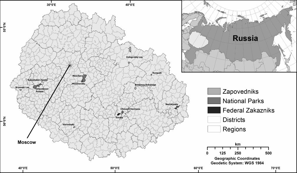
Our study area includes 12 federally protected areas covering 4,045 km2 in the temperate
forest zone of European Russia: 6 strict and 6 multiple use areas (Figure 1). This total area is
about one-third the size of the protected areas system in Costa Rica (Pfaff et al. 2009) and
slightly larger than the total land and water area of the U.S. state of Rhode Island. The average
strict protected area in our sample is 191 km2 in size; multiple use areas tend to be larger, with an
average size of 483 km2. The date of establishment of these 12 protected areas varies between
1989 and 2006 (Table 1). While there were some protected areas in our study region established

13
prior to the collapse of the Soviet Union, we only analyze post-Soviet protected areas in order to
provide a fair assessment of panel methods.
<Figure 1>
Central European Russia is a mosaic of agriculture and forest. Agricultural crops include
mostly grains, and the southern part of the study area includes the fertile ‘black soil’ zone. The
forests of Central Russia are made up of deciduous and mixed tree species. Common deciduous
species include lime, oak, birch, aspen, ash, maple and elm. Scotch pine is the dominant
coniferous species. While total forest cover is lower in this region than parts of Northern
European Russia, timber harvesting is still important due to low transportation costs. In
particular, timber harvesting around Moscow city has increased considerably since 2000
(Wendland et al. 2011; Baumann et al. 2012). Population density in Central Russia is also higher
than in other parts of Russia, potentially causing higher threats for protected areas.
Forest Disturbance Data
We define protected area effectiveness as the change in forest disturbance due to
protected area designation. Forest disturbance is measured using remote sensing imagery. Forest
cover is strongly correlated with biodiversity and is the outcome evaluated in most assessments
of protected area effectiveness (e.g., Mas 2005; Andam et al. 2008; Pfaff et al. 2009; Joppa and
Pfaff 2011; Pfaff et al. 2013). While we cannot distinguish forest disturbance events due to
manmade versus natural causes – a limitation in most land-use change analyses – remote sensing
classifications of forest disturbance in European Russia have attributed the majority of
disturbance events to manmade causes such as logging (Potapov, Turubanova and Hansen 2011).
Additionally, the remote sensing data used in this study were visually inspected and any data for
parks and years that were characteristic of a natural event such as flooding or fire were removed.
14
Our measure of forest disturbance comes from 8 Landsat footprints classified for forest
cover change in 5-year increments from 1985 to 2010 (see Baumann et al. 2012). This primary
analysis provides 30-meter resolution data on forest cover change with average accuracies
greater than 90%. We randomly sample 1% of all pixels within each of the 12 protected areas
that were forested according to the 1985 land cover classification. Thus, we take an equal
proportion of pixels from each park. This gives a sample size of about 40,000 protected area
pixels. We then sample 4-times this amount of forested pixels from areas outside of protected
areas. For both samples we specify a minimum distance criterion of 300 meters between pixels to
reduce spatial correlation.
For each pixel selected we record whether it stayed in forest in a given 5-year period
(value of “0”) or whether it was disturbed by forest clearing (“1”). A pixel is removed from the
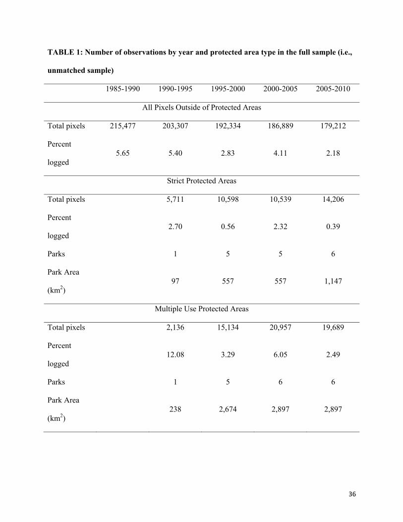
dataset once the forest is disturbed because 20 years is not sufficient time for forest to regenerate
to a harvestable size given an average rotation period of more than 50 years in Russia. Because
pixels are removed once cut, and because new protected areas were created between 1990 and
2010, the total number of observations within and outside of protected areas vary over each time
period (Table 1): in 1985-1990 – before any parks – there are approximately 215,000
unprotected observations, whereas in 2005-2010 there are about 34,000 within protected areas
and 180,000 outside of protected areas.
<Table 1>
Covariates
We select covariates that we assumed to be correlated with both the treatment
(protection) and outcome (forest disturbance), and that are available for our study region. In the
tropics, protected area placement has been found to be highly correlated with remoteness and
15
low economic productivity (Andam et al. 2008; Joppa and Pfaff 2010). Forest disturbance in
European Russia has shown to increasingly be correlated with profit-maximization behaviors
that factor in transportation costs and opportunity costs of the land (Wendland et al. 2011). Thus,
for both of these decisions – protection and forest disturbance – we control for accessibility and
biophysical characteristics of the pixel, as these characteristics strongly influence the net
economic returns from disturbing a forest plot.
Forest disturbance is a capital-intensive activity whose net returns are greatly affected by
accessibility. Since we lack monetized plot-level cost variables, we include multiple physical
proxies of disturbance costs that are related to accessibility. Specific variables include the
distances to forest edge, closest town, Moscow, and closest road; elevation; and slope. Distances
are measured as the Euclidean distance from the pixel to the object and recorded in kilometers.
Datasets on Russian cities with at least 50,000 persons, and major paved roads (circa 1990), are
from the SCANEX Research and Development Center, a Russian remote sensing company. Data
on forest edge is derived from the remote sensing analysis described above, and calculated for
each time period whereas other distance measures did not vary over time. Elevation and slope
data come from NOAA’s Global Land 1-km Base Elevation Project; elevation is measured in
meters and slope as a percent.
There are additional biophysical variables that might be correlated with timber
productivity, such as climate, soil quality or rainfall. Since these physical accessibility indicators
likely influence disturbance returns, the same indicators will also affect protected area status if
regions with low returns to disturbance are systematically more (or less) likely to be protected
than regions with high returns to disturbance. However, variables such as climate and soils are
generally time-invariant over the 25-year period of our study, and the fixed effects estimation

16
strategy (see Section IV) controls for these by placing all variables in difference-in-means form.
As argued below, placing variables in difference-in-means form implicitly controls for all time-
invariant forest disturbance drivers by eliminating them from the model unobservable in
estimation. Since the net returns to forest disturbance can be strongly impacted by time-invariant
physical plot characteristics, panel analysis with plot fixed effects provides a simple way to
control for important drivers of forest disturbance without collecting additional data.
IV. EMPIRICAL STRATEGY
Our objective is to estimate the average treatment effect on the treated (i.e., protected
areas), which is the difference between forest disturbance within protected areas and the
expected effect if the protected area was not there. Mathematically, this is represented by: ∑ 1 0, , (1)
where 1 when a plot, i, is protected and . is the observed outcome with “1” indicating
forest disturbance and “0” otherwise. This gives the amount of forest disturbance prevented
within the boundaries of the parks by protected area status. We estimate treatment effects
separately for strict and multiple use protected areas.
To construct a valid control group we use matching to select the best controls from
observations outside of protected areas (Table 1). For each protected area type we partially
control for administrative influences on forest clearing discussed in Section II by omitting any
control observations that do not fall within the same administrative regions as the protected areas
(see Figure 1). We then use logistic regression on the remaining observations to estimate the
propensity score, i.e., the conditional probability of a treatment (i.e., protected area observation)
or control observation being designated as a park. Specifically, we estimate: 1 , (2)

17
where are the observable covariates described in Section III; and is the logistic function.
The estimated propensity scores are then used to match treatment to control observations
using nearest neighbor 1-to-1 matching without replacement as suggested by Rubin (2006). To
match the data, we estimate the propensity score (Equation 2) for each protected area type using
the 1985 remote sensing data – before any of the protected areas were designated in our study.
Thus, we assume that 1985 matched treatment-control observations remain good matches
through all time periods. We implement matching using the PSMATCH2 algorithm in Stata11
(Leuven and Sianesi 2003).i We restrict the maximum distance between matches using a caliper
size of a quarter of the standard deviation of the estimated propensity score as recommended by
Guo and Fraser (2010).
To ensure that matching improves similarity between treatment and control observations,
we check covariate balance in our samples before and after matching by calculating the
difference in means normalized by the square root of the sum of the variances, which is
preferable over the t-statistic when there are large differences in sample size (Imbens and
Wooldridge 2009). Specifically, we estimate: ⁄ , (3)
where is the mean, the variance, “1” designates areas within protected areas and “2” areas
outside of protected areas. The rule of thumb is that a normalized difference in means greater
than 0.25 can bias regression estimation (Imbens and Wooldridge 2009).
We estimate post-matching linear regressions for each time period as: _ , (4)
where t indicates the time period (i.e., 1985-1990, etc.); is “1” if plot i is disturbed in time t
and “0” otherwise; consists of the set of time-invariant independent variables (e.g., distance to
18
Moscow) contained within the larger set of previously described covariates ; time-varying
independent variables are protected area status ( ) and distance to the forest edge
( _ ); are plot effects; and is a vector of year fixed effects used to control for
variations over time that affect all observations (e.g., national timber prices, exchange rates, etc.).
Estimated parameter vectors include the set , , , , , . The parameter vectors and are
used to form the average marginal effects of a protected area on the plot-level probability of
forest disturbance accounting for the interactions between protection status and time dummies.
A key identification question is how to handle the plot effect , which includes all time-
invariant plot-level omitted variables. These omitted variables can bias the parameter if they
are correlated with both the likelihood of being a protected area and forest disturbance. For
example, we lack good data on a plot’s soil quality and the micro-climate in which the plot
resides. Soils and micro-climatic conditions can influence the type of tree species that can be
grown, and hence, timber yields. Such unobservables are likely to be time-invariant over the 25
years of our data, and could influence protected area decisions if the government is looking to
conserve particular forest types. These unobservables can induce bias if the plot effect is
modeled as a random effect. However, modeling the plot effect as a fixed effect provides a way
to control for any such time-invariant unobservable and observable drivers of forest disturbance.
By writing equation (4) in differences-in-means form (known as the within estimator), all time-
invariant variables are eliminated (including ), while all parameters on time-varying variables
are preserved. Only parameters on time-varying independent variables can be identified when
plot fixed effects are modeled; in our case these are only the distance to forest edge and the
protected area dummy. We estimate Equation 4 as a linear probability model in both random and
fixed effects form.
19
Our inclusion of an interaction between the park dummy variable and the vector of year
fixed effects allows the marginal effect of protected area status to vary by time period, an
important feature given the large temporal variation in policy factors affecting timber
management and conservation budgets from 1990 to 2010 in European Russia. All estimations
include standard errors clustered at the district level (see Figure 1). Cluster robust standard errors
allow spatial correlation across units, in our case, correlation across pixels within the same
district. The district level is important for forest management decisions (see Section II) and
provides a reasonable spatial distance to allow correlation across units without imposing strong
distributional assumptions on the data. Additionally, we follow Pfaff et al. (2009) and Pfaff et al.
(2013) in testing for heterogeneity effects across parks by estimating Equation 4 for parks above
and below the median distances to Moscow and nearest road, important physical indicators of
forest disturbance threats.
We choose a linear probability model over non-linear Probit or Logit models for two
reasons. First, plot fixed effects cannot be easily included in non-linear discrete-choice models in
a flexible manner. Fixed plot effects cannot be included in a Probit model due to the incidental
parameters problem, and fixed effects Logit models do not allow for calculation of marginal
effects since marginal effects are non-linear functions of the un-estimated fixed effects (see
Wooldridge 2010, Ch. 15). Further, while correlated random effects estimation can be used in
non-linear models to introduce some correlation between a plot-level random effect and the park
dummy variable (see Cameron and Trivedi 2005, Ch. 23), one must assume a particular
distribution for the plot effect. In contrast, the fixed effect linear probability model is robust to
any distributional assumption of the plot effect – as the plot effect is entirely differenced out of
the model. Second, while linear probability models have the obvious weakness of not
20
constraining probabilities between zero and one, many researchers have shown that they give
almost identical marginal effects at the mean of the data as do non-linear Probit or Logit models
with similar identifying assumptions (see Angrist and Pischke 2009, Ch. 3; Wooldridge 2010,
Ch. 15). Since our primary interest is in estimating marginal effects, we choose the more flexible
fixed effects linear probability model for estimation.
V. RESULTS
The remote sensing analysis shows that forest disturbance probabilities in our sample of
pixels outside of protected areas range between 2 and 6 percentage points over a 5-year time
period (Table 1). Disturbance rates have generally fallen since the collapse of the Soviet Union,
with an increase in disturbance in 2000-2005 that corresponds to the end of the Asian financial
crisis (1998) and the beginning of Putin’s presidency (2001). These temporal patterns in forest
disturbance are consistent with reports on logging trends in post-Soviet Russia (Torniainen,
Saastamoinen and Petrov 2006) and remote sensing analyses of forest cover in European Russia
(Potapov, Turubanova and Hansen 2011; Baumann et al. 2012). Considering the rate of forest
disturbance in protected areas over time, it fluctuates in both strict and multiple use protected
areas in a similar pattern to that outside of protected areas (Table 1). However, strict protected
areas have a lower rate and multiple use protected areas a higher rate of forest disturbance than
areas outside of protected areas.
Considering where protected areas are located, descriptive statistics suggest differences
across park types and controls (Table 2). Strict protected areas are more likely to be farther from
the forest edge, closest town and road than the average control observation, indicating
remoteness. But, they are closer to Moscow, have lower elevations and less steep slopes than
control observations; factors that could lead to more harvesting. Multiple use areas tend to be
21
farther from roads, farther from Moscow and at lower elevations than observations outside of
protected areas (Table 2). However, these parks are on average closer to the forest edge and
nearest town than the average control observation, indicating that they are in closer proximity to
logging threats.
<Table 2>
A more formal test of differences among treatment groups and controls is the difference
in means (Table 3). For both strict and multiple use protected areas, several covariates have
differences in means exceeding the rule of thumb of 0.25, indicating that simple regression
analysis without matching is likely biased (Imbens and Wooldridge 2009). After matching, the
covariate balance is greatly improved for all covariates and both protected area types (Table 3).
The slight remaining differences in means further motivate the use of post-matching multivariate
regression analysis.
<Table 3>
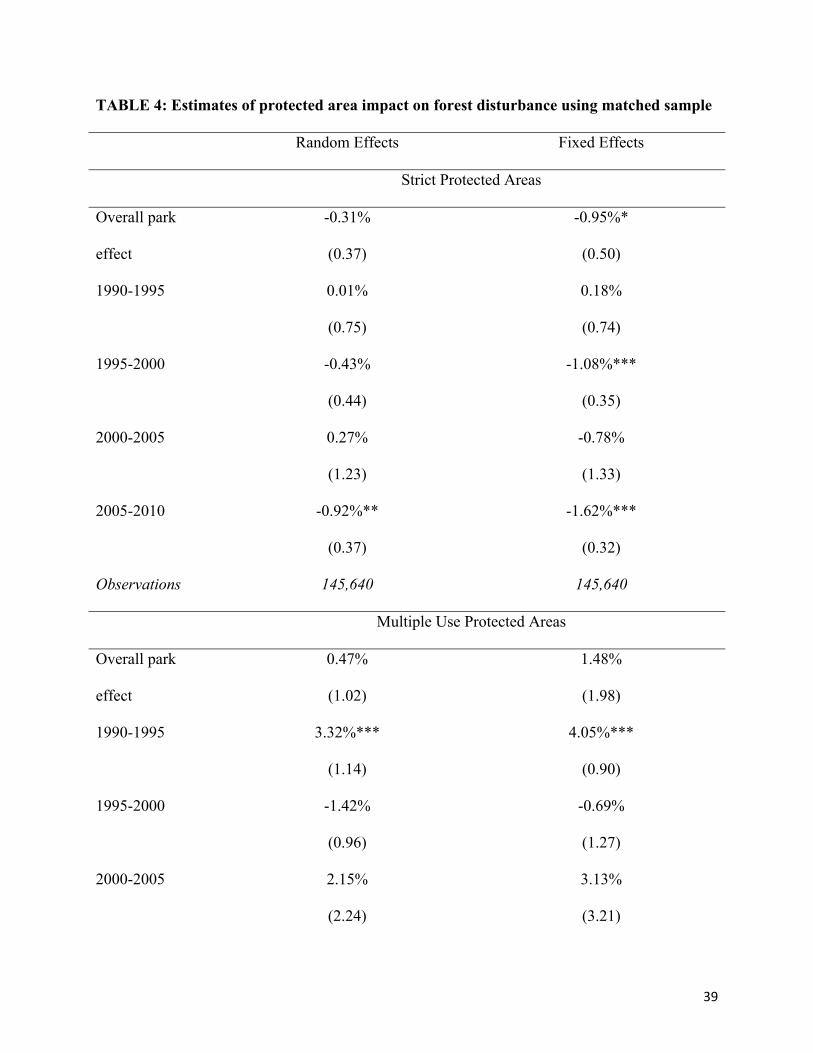
The impact estimates for strict protected areas suggest a negative and statistically
significant effect of 1 to 2 percentage points over a 5-year time period in some periods, and no
effect in others (Table 4). The negative sign indicates that strict protected areas experience less
forest disturbance than comparable control observations. The estimated effects are statistically
significant in 1995-2000 and 2005-2010, periods with the lowest rates of disturbance in the
overall sample (Table 1). Random and fixed effects estimators give reasonably similar
qualitative results for most time periods, though there is a divergence in the qualitative and
quantitative result for whether parks are effective or not in 1995-2000. Estimated as an overall
treatment effect (i.e., no time interactions), we find a park effect of about 1 percentage point,
weakly significant at the 90% level using fixed effects, and no significant effect using random
22
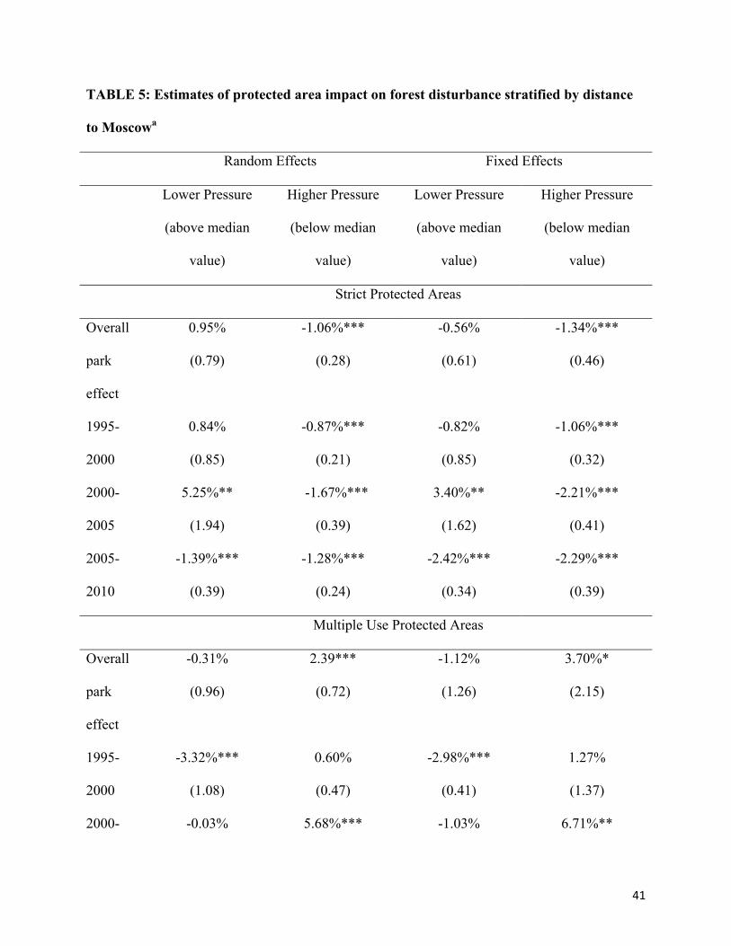
effects. When we estimate the effect of strict protected areas based on their location we find
differences across parks located closer to or farther away from Moscow (Table 5).ii We find that
parks closer to Moscow (higher pressure) reduce forest disturbance more than parks farther from
Moscow (lower pressure). The overall effect is about 1 percentage point, with 5-year effects
ranging from 1 to 2 percentage points. Magnitudes differ considerably among estimators, and we
come back to this issue in the discussion. The difference across parks located closer to or farther
away from nearest roads was similar to that found for distance to Moscow: parks closer to a road
reduced disturbance by about 1 percentage point – significant at the 95% level – compared to no
statistical effect for parks farther from roads (results not reported in table).
<Table 4>
<Table 5>
In contrast, we find few statistically significant impacts of multiple use protected areas on
forest disturbance (Table 4). The overall effect from the fixed effects estimator is positive but not
significant. The estimated effect is insignificant across most time periods, with the exception of
the 1990-1995 time period. There is only one park in this period (Table 1), so this effect is
specific to only that park. Between the random and fixed effects estimators, the qualitative
results are similar. When we stratify multiple use parks by distance to Moscow we find that,
overall, parks closer to Moscow experience an increase in forest disturbance compared to areas
outside of parks (Table 5); however, this overall park effect seems driven by the large,
statistically significant effect during the 2000-2005 period (end of the Asian financial crisis and
the start of Putin’s leadership). The effect of parks farther from Moscow is mostly negative,
though significantly different from zero only during the 1995-2000 period. We do not find any
difference across multiple use parks located closer to or farther away from a road (results not
23
reported in table).
VI. DISCUSSION
We set out to do two things in this paper: (1) provide the first quantitative assessment of
the effectiveness of protected areas in post-Soviet European Russia at reducing forest
disturbance, and (2) evaluate whether including plot fixed effects into panel estimators (rare in
the environmental program evaluation literature) generate significantly different estimates from
estimators without plot fixed effects. We address each of these in turn below.
The effect of post-Soviet protected areas in European Russia appears highly correlated
with the type of park – strict or multiple use – as these vary in their location, management,
funding and permitted uses. This is similar to protected area effectiveness in the tropics where
the type of protection, which is correlated with the location of the protected area and allowable
uses, also influences the magnitude of the effect (Pfaff et al. 2009; Nelson and Chomitz 2011;
Pfaff et al. 2013). In European Russia, strict protected areas are located in more remote locations,
have more funding and better enforcement, and do not permit logging. They appear to have had
some impact on lowering forest disturbance compared to similar observations located outside of
protection. While this impact may appear small – ranging from 1 to 2 percentage points over a 5-
year time period – it is comparable to findings of a global evaluation of protected area
effectiveness (Joppa and Pfaff 2011) and is reflective of the overall low rate of forest disturbance
in our study region, which ranges between 2 and 5 percent for a 5-year time period between 1990
and 2010.
Interestingly, the time periods when strict protected areas are most effective are also the
periods with the lowest overall disturbance rates in our study: 1995-2000 and 2005-2010.
Protected area effectiveness depends on two things: the presence of threat and the ability to block
24
this threat. Since the amount of threat or pressure does not appear to be increasing in these time
periods based on forest disturbance rates outside of protected areas (Table 1), the statistically
significant effect of strict protected areas may be due to an increased ability to block pressures.
As noted in Section II, there have been a number of changes in forest and protected area
governance and funding in Russia between 1990 and 2010, and the heterogeneity in our
effectiveness estimates are likely related to some of those changes. The result that strict protected
areas located closer to Moscow (or roads) have a larger impact than parks located farther away is
consistent with findings in the tropics that show that parks located closer to threats have higher
impact estimates (Pfaff et al. 2009; Pfaff et al. 2013). Overall, while located in areas less likely
to face forest disturbance, strict protected areas in post-Soviet Russia seem to be blocking a good
proportion of the threats they do encounter.
In contrast, multiple use protected areas in post-Soviet European Russia do not appear to
have much impact on forest disturbance. The reason for this is not a lack of forest disturbance
threat though: in contrast to strict protected areas these parks tend to be located in locations more
susceptible to logging (Table 2) and have higher rates of disturbance (Table 1). Thus, we
conclude that they are not blocking disturbance threats. This finding is in contrast to results
found in tropical country studies that show multiple use areas have larger impacts on lowering
deforestation than strict protected areas because there is more threat to block (Pfaff et al. 2013),
or at least are as effective as strict protected areas (Nolte et al. 2013). The low effectiveness of
Russia’s multiple use areas may be due to federally permitted logging leases to private firms, or
may be indicative of illegal activity, such as the sanitary logging practice conducted by the
Federal Forest Service. As noted in Section II, both types of multiple use areas permit logging,
and there have been perverse incentives for local forestry officials to allow logging on federal

25
lands to generate revenue for their own budgets. Of course, there is also a shortage of funding
and management noted for multiple use areas in post-Soviet Russia, indicating that illegal
logging within these boundaries is possible. While it appears that parks located closer to Moscow
are more likely to have forest disturbance within their borders, albeit only in one time period, this
does not shed much light on whether this reflects legally permitted (since transportation costs
would be lower) or illegal (since pressure to take logs would be higher) disturbance.
Our estimated impacts of post-Soviet European Russia protected areas are important to
bear in mind as a recent GAP analysis for conservation in Russia has proposed the creation of an
additional 403 federally protected areas (Krever, Stishov and Onufrenya 2009). Multiple use
protected areas, such as national parks and federal zakazniks, make up the majority of the
proposed new protected areas. Our results raise questions about enforcement against illegal
logging and or possible permitted logging operations within multiple use areas. At best, current
multiple use areas are a zero sum game, in that they neither increase nor decrease forest
disturbance relative to similar areas outside of protection. Before any new multiple use areas are
created, there is a need for on-the-ground research to understand why these park types appear to
be susceptible to forest disturbance. For the creation of new strict protected areas, policy
recommendations would be that locating these types of parks closer to areas likely to experience
threats (closer to major cities or roads, for example) would provide the most additional benefit.
We turn next to the methodological evaluation of including plot fixed effects into panel
estimators for impact evaluation. The number of impact evaluations is growing in the
conservation and environment field (Pattanayak, Wunder and Ferraro 2010; Ferraro 2011). The
most common approach is to use matching to construct a valid control group and then cross-
sectional regression to estimate the treatment effect. Recent studies using this method to estimate
26
the impact of protected areas include: Andam et al. (2008), Pfaff et al. (2009), Ferraro and
Hanauer (2010), Joppa and Pfaff (2011), Nelson and Chomitz (2011), Nolte et al. (2013), and
Pfaff et al. (2013). There is also an increasing interest in using program evaluation methods to
estimate the impact of payments for ecosystem services programs (e.g., Pfaff, Robalino and
Sanchez-Azofeifa 2008; Uchida, Rozelle and Xu 2009; Robalino and Pfaff 2013), and some of
these studies have used fixed effect panel methods to estimate treatment effects on forest
protection (see Alix-Garcia, Shapiro and Sims 2012b; Arriagada et al. 2012). A relevant question
is whether moving to the panel data structure is critical for robust estimates of treatment effects?
While random effects estimates differ from cross-sectional regression in the modeling of serial
correlation in the unobservables, the identification assumptions are identical across both
estimators. We interpret random effects estimates of protected area effectiveness as
methodologically similar to the conventional environmental program evaluation literature.
The inclusion of plot fixed effects generates significant differences in effectiveness
estimates for strict protected areas, and less so for multiple use areas, when compared with
random effects estimates. Hausman tests confirm the statistical difference across fixed and
random effects estimates (5% level).iii While the magnitude of the difference in the effectiveness
estimates between fixed and random effects seems small in absolute probability terms, fixed
effects estimates are 2.5 times larger for 1995-2000 and 1.8 times larger for 2005-2010 for strict
protected areas (Table 4). Taking the 2005-2010 estimates and park area as an example for
context, the effectiveness estimates from fixed effects indicate that strict protected areas prevent
approximately 111 km2 of disturbance over a 30-year time horizon, while the corresponding
random effects estimates is only 63 km2. Since both estimators use the same sample, differences
between fixed and random effects imply that time-invariant plot unobservables are correlated
27
with protected area status. The presence of such unobservables can bias post-matching regression
estimates of conservation effectiveness.
While bias from time-invariant unobservables could be reduced in cross-sectional post-
matching regressions by collecting more data on plot characteristics or instrumenting for
protection, such data is not always easily available or well-measured, and protection instruments
are often far from obvious (see Sims 2010 for an example of an instrumental variables approach
to protected area impacts). Our results suggest that building better temporal variation with spatial
land-use / land-cover data can reduce the number of assumptions required for identification of
protected area – or other environmental programs – effectiveness. The identification of park
effectiveness with plot fixed effects relies on (1) repeated remote sensing landscape images over
time, and (2) temporal variation in the location of protected areas (or other environmental
programs) within the time-frame of the estimation sample. The incorporation of similar panel
methods into evaluations of environmental policy on land use is becoming increasingly feasible
given release of the Landsat archives (Goward et al. 2006; Blackman 2013) and the advancement
of remote sensing techniques to provide temporally-rich land cover change classifications
(Huang et al. 2008, 2009).

28
REFERENCES
Alix-Garcia, Jennifer, Tobias Kummerle, and Volker C. Radeloff. 2012a. “Prices, land tenure
institutions, and geography: A matching analysis of farmland abandonment in post-
Socialist Eastern Europe.” Land Economics 88 (3): 425-433.
Alix-Garcia, Jennifer M., Elizabeth N. Shapiro, and Katharine R.E. Sims. 2012b. “Forest
conservation and slippage: evidence from Mexico’s national payments for ecosystem
services program.” Land Economics 88 (4): 613-638.
Andam, Kwaw S., Paul J. Ferraro, Alexander Pfaff, G. Arturo Sanchez-Azofeifa, and Juan A.
Robalino. 2008. “Measuring the effectiveness of protected area networks in reducing
deforestation.” Proceedings of the National Academy of Sciences 105 (42): 16089-16094.
Angrist, Joshua D., and Jorn-Steffen Pischke. 2009. “Mostly Harmless Econometrics: An
Empiricist’s Companion.” Princeton University Press.
Arriagada, Rodrigo A., Paul J. Ferraro, Erin O. Sills, Subhrendu K. Pattanayak, and Silvia
Cordero-Sancho. 2012. “Do payments for environmental services affect forest cover? A
farm-level evaluation from Costa Rica.” Land Economics 88 (2): 382-399.
Baumann, Matthias, Mutlu Ozdogan, Tobias Kuemmerle, Kelly J. Wendland, Elena Esipova, and
Volker C. Radeloff. 2012. “Using the Landsat record to detect forest-cover changes
during and after the collapse of the Soviet Union in the temperate zone of European
Russia.” Remote Sensing of Environment 124: 174-184.
Blackman, Allen. 2013. “Evaluating forest conservation policies in developing countries using
remote sensing data: An introduction and practical guide.” Forest Policy and Economics
34: 1-16.
29
Brooks, Thomas M., Mohamed I. Bakarr, Tim Boucher, Gustavo A.B. Da Fonseca, Craig Hilton-
Taylor, Jonathan M. Hoekstra, Tom Moritz, Silvio Olivieri, Jeff Parrish, Robert L.
Pressey, Ana S.L. Rodrigues, Wes Sechrest, Ali Stattersfield, Wendy Strahm, and Simon
N. Stuart. 2004. “Coverage provided by the global protected-area system: is it enough?”
Bioscience 54 (12): 1081-1091.
Bruner, Aaron G., Raymond E. Gullison, Richard E. Rice, and Gustavo A.B. da Fonseca. 2001.
“Effectiveness of parks in protecting tropical biodiversity.” Science 291: 125-128.
Cameron, A. Colin, and Pravin K. Trivedi. 2005. “Microeconometrics: Methods and
Applications.” Cambridge University Press, New York.
Colwell, Mark A., Alexander V. Dubynin, Andrei Y. Koroliuk, and Nikolai A. Sobolev. 1997.
“Russian nature reserves and conservation of biological diversity.” Natural Areas
Journal 17: 56-68.
Dudley, Nigel, Biksham Gujja, Bill Jackson, Jean-Paul Jeanrenaud, Gonzalo Oviedo, Adrian
Phillips, Pedro Rosabel, Sue Stolton, and Sue Wells. 1999. “Challenges for Protected
Areas in the 21st Century.” In: Stolton, Sue, and Nigel Dudley (Eds.), Partnerships for
Protection, Earthscan Publication, London.
Eikeland, Sveinung, Einar Eythorsson, and Lyudmila Ivanova. 2004. “From management to
mediation: local forestry management and the forestry crisis in post-socialist Russia.”
Environmental Management 33 (3): 285-293.
Ferraro, Paul J. 2009. “Counterfactual thinking and impact evaluation in environmental policy.”
New Directions for Evaluation 122: 75–84.
Ferraro, Paul J. 2011. “The future of payments for environmental services.” Conservation
Biology 25: 1134-1138.

30
Ferraro, Paul J., and Merlin M. Hanauer. 2011. “Protecting ecosystems and alleviating poverty
with parks and reserves: ‘win-win’ or tradeoffs?” Environmental and Resource
Economics 48 (2): 269-286.
Ferraro, Paul J., and Subhrendu K. Pattanayak. 2006. “Money for nothing? A call for empirical
evaluation of biodiversity conservation instruments.” PLoS Biology 4: e105.
Goward, Samuel, Terry Arvidson, Darrel Williams, John Faundeen, James Irons, and Shannon
Franks. 2006. “Historical record of Landsat global coverage: Mission operations,
NSLRSDA, and international cooperator stations.” Photogrammetric Engineering and
Remote Sensing 72: 1155–1169.
Guo, Shenyang, and Mark W. Fraser. 2010. “Propensity score analysis: statistical methods and
applications.” Sage Publications, Washington, D.C.
Huang, Chenguan, Kuan Song, Sunghee Kim, John R.G. Townshend, Paul Davis, Jeffrey G.
Masek, and Samuel N. Goward. 2008. “Use of a dark object concept and support vector
machines to automate forest cover change analysis.” Remote Sensing of Environment
112: 970–985.
Huang, Chenguan, Samuel N. Goward, Jeffrey G. Masek, Feng Gao, Eric F. Vermote, Nancy
Thomas, Karen Schleeweis, Robert E. Kennedy, Zhiliang Zhu, Jeffrey C. Eidenshink, and
John R.G. Townshend. 2009. “Development of time series stacks of Landsat images for
reconstructing forest disturbance history.” International Journal of Digital Earth 2 (3):
195–218.
Imbens, Guido M., and Jeffrey M. Wooldridge. 2009. “Recent developments in the econometrics
of program evaluation.” Journal of Economic Literature 47: 5-86.
31
Jenkins, Clinton N., and Lucas Joppa. 2009. “Expansion of the global terrestrial protected area
system.” Biological Conservation 142 (10): 2166-2174.
Joppa, Lucas, and Alexander Pfaff. 2009. “High and far: Biases in the location of protected
areas.” PLoS One 4: e8273.
Joppa, Lucas, and Alexander Pfaff. 2010. “Reassessing the forest impacts of protection: The
challenge of nonrandom location and a corrective method.” Annals of the New York
Academy of Sciences 1185: 135-149.
Joppa, Lucas, and Alexander Pfaff. 2011. “Global protected area impacts.” Proceedings of the
Royal Society 278 (1712): 1633-1638.
Kortelainen, Jarmo, and Juha Kotilainen. 2003. “Ownership changes and transformation of the
Russian pulp and paper industry.” Eurasian Geography and Economics 44 (5): 384–402.
Krever, Vladimir, Mikhail Stishov, and Irina Onufrenya. 2009. “National protected areas of the
Russian Federation: GAP analysis and perspective framework.” WWF, Moscow.
Krott, Max, Ilpo Tikkanen, Anatoly Petrov, Yuri Tunystsya, Boris Zheliba, Volker Sasse, Irina
Rykounina, and Tarus Tunytsya. 2000. “Policies for Sustainable Forestry in Belarus,
Russia and Ukraine.” European Forest Institute Research Report No. 9. Koninklijke Brill
NV, Leiden.
Leuven, Edwin, and Barbara Sianesi. 2003. “PSMATCH2: Stata Module to Perform Full
Mahalanobis and Propensity Score Matching, Common Support Graphing, and Covariate
Imbalance Testing.” http://ideas.repec.org/c/boc/bocode/ s432001.html.
Mas, Jean-Francois. 2005. “Assessing protected area effectiveness using surrounding (buffer)
areas environmentally similar to the target area.” Environmental Monitoring and
Assessment 105: 69-80.
32
Mason, Charles, and Andrew Plantinga. 2011. “Contracting for impure public goods: Carbon
offsets and additionality.” NBER Working Paper #16963.
Naughton-Treves, Lisa, Margaret B. Holland, and Katrina Brandon. 2005. “The role of protected
areas in conserving biodiversity and sustaining local livelihoods.” Annual Review of
Environmental Resources 30: 219-252.
Nelson, Andrew, and Kenneth M. Chomitz. 2011. “Effectiveness of strict vs. multiple use
protected areas in reducing tropical forest fires: a global analysis using matching
methods.” PLoS ONE 6: e22722.
Nolte, Christoph, Arun Agrawal, Kirsten M. Silvius, and Britaldo S. Soares-Filho. 2013.
“Governance regime and location influence avoided deforestation success of protected
areas in the Brazilian Amazon.” Proceedings of the National Association of Sciences 110
(13): 4956-4961.
Nysten-Haarala, Soili. 2001. “Russian property rights in transition.” International Institute for
Applied Systems Analysis Interim Report IR-01-006. Laxenburg, Austria.
Ostergren, David, and Peter Jacques. 2002. “A political economy of Russian nature conservation
policy: Why scientists have taken a back seat.” Global Environmental Politics 2 (4): 102-
124.
Pappila, Minna. 1999. “The Russian Forest Sector and Legislation in Transition.” International
Institute for Applied Systems Analysis IR-99-058. Laxenburg, Austria.
Pattanayak, Subhrendu K., Sven Wunder, and Paul J. Ferraro. 2010. “Show me the money: do
payments supply environmental services in developing countries?” Review of
Environmental Economics and Policy 4: 254-274.
33
Pfaff, Alexander, Juan Robalino, and G. Arturo Sanchez-Azofeifa. 2008. “Payments for
environmental services: Empirical analysis for Costa Rica.” Working Paper Series
SAN08–05, Terry Sanford Institute of Public Policy, Duke University, Durham, NC.
Pfaff, Alexander, Juan Robalino, G. Arturo Sanchez-Azofeifa, Kwaw S. Andam, and Paul J.
Ferraro. 2009. “Park location affects forest protection: Land characteristics cause
differences in park impacts across Costa Rica.” The B.E. Journal of Economic Analysis
and Policy 9 (2): 1-24.
Pfaff, Alexander, Juan Robalino, Eirivelthon Lima, Catalina Sandoval, and Luis D. Herrera.
2013. “Governance, location and avoided deforestation from protected areas: greater
restrictions can have lower impact, due to differences in location.” World Development,
in press. Online: http://www.sciencedirect.com/science/article/pii/S0305750X1300017X.
Potapov, Peter, Svetlana Turubanova, and Matthew C. Hansen. 2011. “Regional-scale boreal
forest monitoring using Landsat data composites: first results for European Russia.”
Remote Sensing of Environment 115: 548-561.
Prishchepov, Alexander V., Volker C. Radeloff, Matthias Baumann, Tobias Kuemmerle, and
Daniel Muller. 2012. “Effects of institutional changes on land use: agricultural land
abandonment during the transition from state-command to market-driven economies in
post-Soviet Europe.” Environmental Research Letters DOI:10.1088/1748-
9326/7/2/024021.
Pryde, Philip R. 1997. “Post-Soviet development and status on Russian nature reserves.” Post-
Soviet Geography and Economics 38 (2):63-80.

34
Radeloff, Volker C., Fred Beaudry, Thomas M. Brooks, Van Butsic, Maxim Dubinin, Tobias
Kuemmerle, and Anna M. Pidgeon. 2013. “Hot moments for biodiversity conservation.”
Conservation Letters 6 (1): 58-65.
Robalino, Juan, and Alexander Pfaff. 2013. “Ecopayments and deforestation in Costa Rica: A
nationwide analysis of PSA’s initial years.” Land Economics 89(3): 432-448.
Rodrigues, Ana S.L., H. Resit Akcakaya, Sandy A. Andelman, Mohamed I. Bakarr, L. Boitani,
Thomas M. Brooks, Janice S. Chanson, Lincoln D.C. Fishpool, Gustavo A.B. Da
Fonesca, Kevin J. Gaston, Michael Hoffmann, Pablo A. Marquet, John D. Pilgrim,
Robert L. Pressey, Jan Schipper, Wes Sechrest, Simon N. Stuart, Les G. Underhill,
Robert W. Waller, Matthew E.J. Watts, and Xie Yan. 2004. “Global GAP analysis:
priority regions for expanding the global protected-area network.” Bioscience 54(12):
1092-1100.
Rubin, Donald B. 2006. “Matched Sampling for Causal Effects.” Cambridge University Press,
New York.
Scharlemann, Jorn P.W., Valerie Kapos, Alison Campbell, Igor Lysenko, Neil D. Burgess,
Matthew C. Hansen, Holly K. Gibbs, Barney Dickson, and Lera Miles. 2010. “Securing
tropical forest carbon: the contribution of protected areas to REDD.” Oryx 44 (3): 352-
357.
Sims, Katherine R.E. 2010. “Conservation and development: Evidence from Thai protected
areas.” Journal of Environmental Economics and Management 60 (2): 94-114.
Sobolev, Nikolai A., Evgeny A. Shvarts, Mikhail L. Kreindlin, Vadim O. Mokievsky, and
Victor A. Zubakin. 1995. “Russia’s protected areas: a survey and identification of
development problems.” Biodiversity and Conservation 4 (9): 964-983.
35
Torniainen, Tatu J., Olli J. Saastamoinen, and Anatoly P. Petrov. 2006. “Russian forest policy in
the turmoil of the changing balance of power.” Forest Policy and Economics 9 (4): 403-
416.
Uchida, Emi, Scott Rozelle, and Jintao Xu. 2009. “Conservation payments, liquidity constraints,
and off-farm labor: Impact of the Grain-for-Green program on rural households in
China.” American Journal of Agricultural Economics 91: 70–86.
Wells, Michael P., and Margaret D. Williams. 1998. “Russia’s protected areas in transition: The
impacts of perestroika, economic Reform and the move towards democracy.” Ambio 27
(3): 198-206.
Wendland, Kelly J., David J. Lewis, Jennifer Alix-Garcia, Mutlu Ozdogan, Matthias Baumann,
and Volker C. Radeloff. 2011 “Regional- and district-level drivers of forest disturbance
in European Russia after the collapse of the Soviet Union.” Global Environmental
Change 21: 1290-1300.
Wendland, Kelly J., David J. Lewis, and Jennifer Alix-Garcia. 2013. “The effect of decentralized
governance on timber extraction in European Russia.” Environmental and Resource
Economics DOI 10.1007/s10640-013-9657-8.
Wooldridge, Jeffrey M., 2010. “Econometric analysis of cross section and panel data.” MIT
Press.
36
TABLE 1: Number of observations by year and protected area type in the full sample (i.e.,
unmatched sample)
1985-1990 1990-1995 1995-2000 2000-2005 2005-2010
All Pixels Outside of Protected Areas
Total pixels 215,477 203,307 192,334 186,889 179,212
Percent
logged 5.65 5.40 2.83 4.11 2.18
Strict Protected Areas
Total pixels 5,711 10,598 10,539 14,206
Percent
logged 2.70 0.56 2.32 0.39
Parks 1 5 5 6
Park Area
(km2) 97 557 557 1,147
Multiple Use Protected Areas
Total pixels 2,136 15,134 20,957 19,689
Percent
logged 12.08 3.29 6.05 2.49
Parks 1 5 6 6
Park Area
(km2) 238 2,674 2,897 2,897

37
TABLE 2: Summary statistics for protected areas and areas outside of protection
Variable All Pixels Outside of
Protected Areas
Strict Protected
Areas
Multiple Use Protected
Areas
Mean
(Std dev)
Mean
(Std dev)
Mean
(Std dev)
Distance to forest edgea
(km)
0.23
(0.28)
0.35
(0.39)
0.19
(0.21)
Distance to closest
town (km)
74.45
(47.74)
99.11
(55.47)
59.37
(25.85)
Distance to Moscow
(km)
443.62
(247,59)
403.95
(161.35)
528.33
(352.79)
Distance to closest road
(km)
1.19
(1.06)
1.57
(1.23)
1.50
(1.28)
Elevation (m) 154.15
(40.77)
150.86
(44.98)
136.46
(47.13)
Slope (%) 1.27
(1.41)
1.06
(1.18)
1.38
(2.15)
Observationsb 215,477 15,441 24,752
aDistance to forest edge in 1985.
bSummary statistics are based on total number of pixels sampled within protected areas and outside of protected
areas (i.e., before matching) in 1985. If observation was ever a protected area (i.e., became a protected area in 1995,
2000, etc.) it was summarized in the protected area column.

38
TABLE 3: Covariate balance using normalized difference in meansa
Variable Strict Protected Areas versus
Controls Multiple Use Areas versus Controls
Unmatchedb Matchedc Unmatchedb Matchedc
Distance to forest
edge 1985 0.23 0.05 -0.11 -0.05
Distance to
closest town 0.16 -0.04 -0.13 0.02
Distance to
Moscow -0.18 0.04 0.17 -0.10
Distance to
closest road 0.33 0.01 0.25 -0.11
Elevation -0.18 0.05 -0.41 -0.11
Slope -0.14 0.01 -0.01 0.02
aNormalized differences are estimated as: difference in the mean values of the covariates across protected area types
and their control groups, normalized by the square root of the sum of the two variances. A negative sign indicates a
smaller value for the protected area and a positive sign indicates a larger value for the protected area. The rule of
thumb is that linear regression methods tend to be sensitive to a normalized difference in mean greater than 0.25
(Imbens and Wooldridge 2009).
bUnmatched sample included all control observations (Table 1, Column 2).
cMatched sample was based on 1-to-1 nearest neighbor matching without replacement using a caliper.
39
TABLE 4: Estimates of protected area impact on forest disturbance using matched sample
Random Effects Fixed Effects
Strict Protected Areas
Overall park
effect
-0.31%
(0.37)
-0.95%*
(0.50)
1990-1995 0.01%
(0.75)
0.18%
(0.74)
1995-2000 -0.43%
(0.44)
-1.08%***
(0.35)
2000-2005 0.27%
(1.23)
-0.78%
(1.33)
2005-2010 -0.92%**
(0.37)
-1.62%***
(0.32)
Observations 145,640 145,640
Multiple Use Protected Areas
Overall park
effect
0.47%
(1.02)
1.48%
(1.98)
1990-1995 3.32%***
(1.14)
4.05%***
(0.90)
1995-2000 -1.42%
(0.96)
-0.69%
(1.27)
2000-2005 2.15%
(2.24)
3.13%
(3.21)

40
2005-2010 -0.08%
(0.50)
1.53%
(1.97)
Observations 184,185 184,185
*** p<0.01, ** p<0.05, * p<0.1
41
TABLE 5: Estimates of protected area impact on forest disturbance stratified by distance
to Moscowa
Random Effects Fixed Effects
Lower Pressure
(above median
value)
Higher Pressure
(below median
value)
Lower Pressure
(above median
value)
Higher Pressure
(below median
value)
Strict Protected Areas
Overall
park
effect
0.95%
(0.79)
-1.06%***
(0.28)
-0.56%
(0.61)
-1.34%***
(0.46)
1995-
2000
0.84%
(0.85)
-0.87%***
(0.21)
-0.82%
(0.85)
-1.06%***
(0.32)
2000-
2005
5.25%**
(1.94)
-1.67%***
(0.39)
3.40%**
(1.62)
-2.21%***
(0.41)
2005-
2010
-1.39%***
(0.39)
-1.28%***
(0.24)
-2.42%***
(0.34)
-2.29%***
(0.39)
Multiple Use Protected Areas
Overall
park
effect
-0.31%
(0.96)
2.39***
(0.72)
-1.12%
(1.26)
3.70%*
(2.15)
1995-
2000
-3.32%***
(1.08)
0.60%
(0.47)
-2.98%***
(0.41)
1.27%
(1.37)
2000- -0.03% 5.68%*** -1.03% 6.71%**

42
2005 (1.43) (1.77) (1.76) (3.18)
2005-
2010
-0.45%
(0.50)
0.86%
(0.76)
-1.25%
(1.11)
3.26%
(2.01)
*** p<0.01, ** p<0.05, * p<0.1
aWe only report park effects after 1995 since there is only one park in the 1990-1995 period (Table 1) for both the strict and multiple use samples.

43
FIGURE 1: Location and names of protected areas

44
i One limitation of propensity score matching is that standard errors are incorrectly estimated; this would lead to
erroneous conclusions of the statistical significance of protected areas if the treatment effect was calculated directly
from the matched data (i.e., through difference in means as implied by Equation 1). However, since we use matching
to preprocess our data and restrict our sample before regression analysis, i.e., we do not use the propensity score
directly to estimate treatment effects, this does not affect our analysis.
iiWhen splitting the sample, we only report park effects after 1995 since there is only one park in the 1990-1995 time
period (Table 1) for both the strict and multiple use samples; splitting the effects for one park across distance to
Moscow or road did not seem relevant for policy implications.
iiiSince we use cluster robust standard errors, the conventional Hausman test of random versus fixed effects is
incorrect since it relies on an assumption that random effects is efficient. We conduct a robust Hausman test using
the linear correlated random effects model with cluster robust standard errors (see Wooldridge 2010, p. 332), which
is also known as the variable addition test for fixed versus random effects.
Recommended