
PUBL0050: Advanced Quantitative Methods
Lecture 5: Panel Data and Difference-in-Differences
Jack Blumenau
1 / 52

Thank you for the feedback!
1. Question: Can we have drop-in hours rather than office hours?• Response: Speak to Constanza!
2. Question: Can we have more advice on merging/cleaning data in R?• Response: I will add some material to the website on how toapproach this.
2 / 52

Thank you for the feedback!
3. Question: Can you provide a crib sheet of R functions?• Response: Anything comprehensive will be difficult, but I will try toadd an overview of the most important functions that we use to thewebsite.
4. Question: Can we have more applied examples of methods?• Response: I will make sure that there are more applications perlecture, even if these are just links to papers.
2 / 52

Thank you for the feedback!
5. Question: Can all lecture notes be put online now?• Response: From reading week, I will upload all slides for the futureweeks, though these are subject to change.
6. Question: Can you provide more help with finding data?• Response: This is a little difficult given the variety of data that youwill all use. I will add some resources of some commonly useddatabases to the website but please do not take this as acomprehensive list! Data sourcing/collection is part of theevaluation.
2 / 52

Thank you for the feedback!
7. Question: What is going to happen with the strike?• Response: I wish I knew.• Real response 1: If the strike goes ahead, I will post the videos of lastyear’s lectures online so that you can watch those.
• Real response 2: We are still trying to work on contingency plans forthe two classes that would be affected by the strike.
2 / 52

Course outline
1. Potential Outcomes and Causal Inference2. Randomized Experiments3. Selection on Observables (I)4. Selection on Observables (II)5. Panel Data and Difference-in-Differences6. Synthetic Control7. Instrumental Variables (I)8. Instrumental Variables (II)9. Regression Discontinuity Designs10. Overview and Review
3 / 52

Was it “the Sun wot won it”?
1992 1997
4 / 52

Was it “the Sun wot won it”?
1992 1997
5 / 52
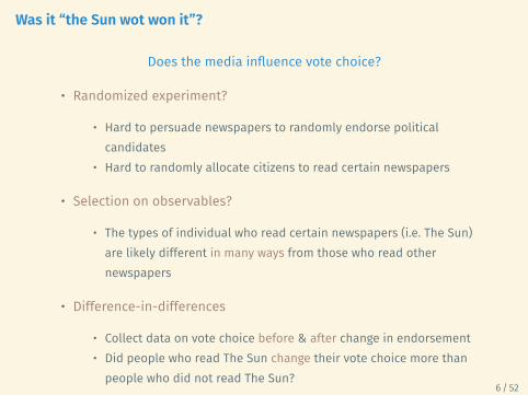
Was it “the Sun wot won it”?
Does the media influence vote choice?
• Randomized experiment?
• Hard to persuade newspapers to randomly endorse politicalcandidates
• Hard to randomly allocate citizens to read certain newspapers
• Selection on observables?
• The types of individual who read certain newspapers (i.e. The Sun)are likely different in many ways from those who read othernewspapers
• Difference-in-differences
• Collect data on vote choice before & after change in endorsement• Did people who read The Sun change their vote choice more thanpeople who did not read The Sun?
6 / 52
Lecture Outline
Difference-in-differences
Regression DD
Threats to Validity
Multiple periods
Conclusion
7 / 52

Difference-in-differences
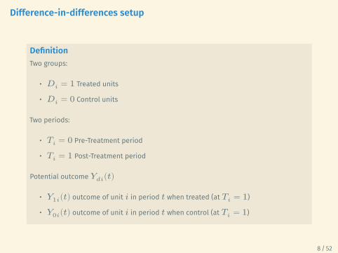
Difference-in-differences setup
DefinitionTwo groups:
• 𝐷𝑖 = 1 Treated units
• 𝐷𝑖 = 0 Control units
Two periods:
• 𝑇𝑖 = 0 Pre-Treatment period
• 𝑇𝑖 = 1 Post-Treatment period
Potential outcome 𝑌𝑑𝑖(𝑡)
• 𝑌1𝑖(𝑡) outcome of unit 𝑖 in period 𝑡 when treated (at 𝑇𝑖 = 1)• 𝑌0𝑖(𝑡) outcome of unit 𝑖 in period 𝑡 when control (at 𝑇𝑖 = 1)
8 / 52
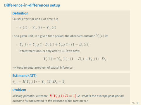
Difference-in-differences setup
DefinitionCausal effect for unit 𝑖 at time 𝑡 is
• 𝜏𝑖(𝑡) = 𝑌1𝑖(𝑡) − 𝑌0𝑖(𝑡)
For a given unit, in a given time period, the observed outcome 𝑌𝑖(𝑡) is:
• 𝑌𝑖(𝑡) = 𝑌1𝑖(𝑡) ⋅ 𝐷𝑖(𝑡) + 𝑌0𝑖(𝑡) ⋅ (1 − 𝐷𝑖(𝑡))• If treatment occurs only after 𝑡 = 0 we have:
𝑌𝑖(1) = 𝑌0𝑖(1) ⋅ (1 − 𝐷𝑖) + 𝑌1𝑖(1) ⋅ 𝐷𝑖
→ Fundamental problem of causal inference.
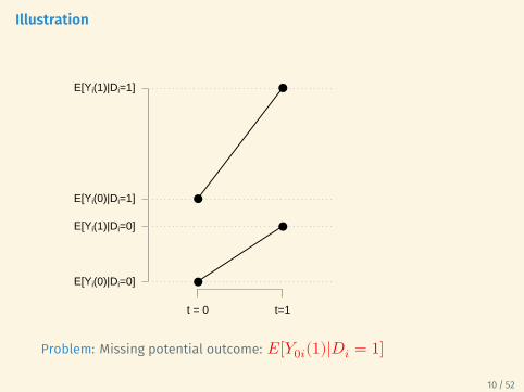
Estimand (ATT)𝜏ATT = 𝐸[𝑌1𝑖(1) − 𝑌0𝑖(1)|𝐷𝑖 = 1]
ProblemMissing potential outcome: 𝐸[𝑌0𝑖(1)|𝐷 = 1], ie. what is the average post-periodoutcome for the treated in the absence of the treatment?
9 / 52
Illustration
Treated vs. control in post-treatment period
t = 0 t=1
E[Yi(0)|Di=0]
E[Yi(1)|Di=0]
E[Yi(0)|Di=1]
E[Yi(1)|Di=1]
●
●
●
●
Problem: Missing potential outcome: 𝐸[𝑌0𝑖(1)|𝐷𝑖 = 1]
10 / 52
Illustration
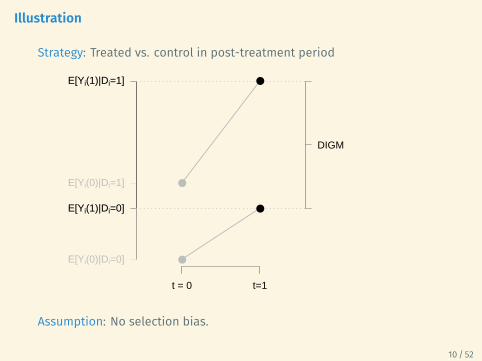
Strategy: Treated vs. control in post-treatment period
t = 0 t=1
E[Yi(0)|Di=0]
E[Yi(1)|Di=0]
E[Yi(0)|Di=1]
E[Yi(1)|Di=1]
E[Yi(1)|Di=0]
E[Yi(1)|Di=1]
DIGM
●
●
●
●
Assumption: No selection bias.
10 / 52
Illustration
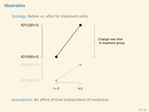
Strategy: Before vs. after for treatment units
t = 0 t=1
E[Yi(0)|Di=0]
E[Yi(1)|Di=0]
E[Yi(0)|Di=1]
E[Yi(1)|Di=1]
E[Yi(0)|Di=1]
E[Yi(1)|Di=1]
Change over time in treatment group
●
●
●
●
Assumption: No effect of time independent of treatment.
10 / 52
Illustration
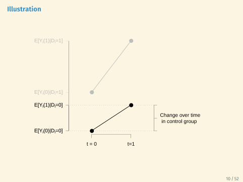
Treated vs. control in post-treatment period
t = 0 t=1
E[Yi(0)|Di=0]
E[Yi(1)|Di=0]
E[Yi(0)|Di=1]
E[Yi(1)|Di=1]
E[Yi(0)|Di=0]
E[Yi(1)|Di=0]
Change over time in control group
●
●
●
●
Treated vs. control in post-treatment period
10 / 52
Illustration
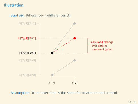
Strategy: Difference-in-differences (1)
t = 0 t=1
E[Yi(0)|Di=0]
E[Yi(1)|Di=0]
E[Yi(0)|Di=1]
E[Yi(1)|Di=1]
E[Yi(0)|Di=1]
E[Y0i(1)|Di=1]
●
●
●
●
●
●
Assumed change over time in treatment group
Assumption: Trend over time is the same for treatment and control.
10 / 52
Illustration
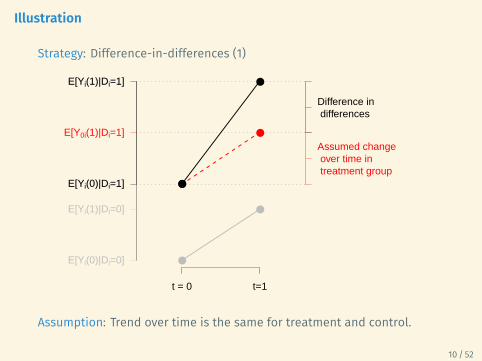
Strategy: Difference-in-differences (1)
t = 0 t=1
E[Yi(0)|Di=0]
E[Yi(1)|Di=0]
E[Yi(0)|Di=1]
E[Yi(1)|Di=1]
E[Yi(0)|Di=1]
E[Yi(1)|Di=1]
E[Y0i(1)|Di=1]
●
●
●
●
●
●
Assumed change over time in treatment group
Difference in differences
Assumption: Trend over time is the same for treatment and control.
10 / 52
Illustration
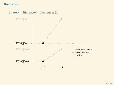
Strategy: Difference-in-differences (2)
t = 0 t=1
E[Yi(0)|Di=0]
E[Yi(1)|Di=0]
E[Yi(0)|Di=1]
E[Yi(1)|Di=1]
E[Yi(0)|Di=0]
E[Yi(0)|Di=1]
Selection bias in pre−treatment period
●
●
●
●
Treated vs. control in post-treatment period
10 / 52
Illustration
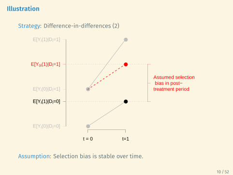
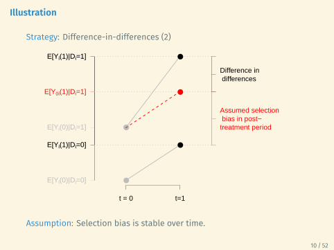
Strategy: Difference-in-differences (2)
t = 0 t=1
E[Yi(0)|Di=0]
E[Yi(1)|Di=0]
E[Yi(0)|Di=1]
E[Yi(1)|Di=1]
E[Yi(1)|Di=0]
E[Y0i(1)|Di=1]
Assumed selection bias in post−treatment period
●
●
●
●
●
●
Assumption: Selection bias is stable over time.
10 / 52
Illustration
Strategy: Difference-in-differences (2)
t = 0 t=1
E[Yi(0)|Di=0]
E[Yi(1)|Di=0]
E[Yi(0)|Di=1]
E[Yi(1)|Di=1]
E[Yi(1)|Di=0]
E[Yi(1)|Di=1]
E[Y0i(1)|Di=1]
Assumed selection bias in post−treatment period
●
●
●
●
●
●
Difference in differences
Assumption: Selection bias is stable over time.
10 / 52
Identification with Difference-in-Differences
Two ways of stating the identifying assumption:
• Parellel trends
• If treated units did not receive the treatment, they would havefollowed the same trend as the control units
• No time-varying confounders
• Omitted variables related both to treatment and outcome must befixed over time
11 / 52
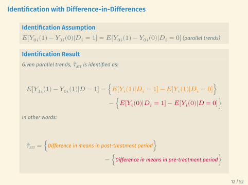
Identification with Difference-in-Differences
Identification Assumption𝐸[𝑌0𝑖(1) − 𝑌0𝑖(0)|𝐷𝑖 = 1] = 𝐸[𝑌0𝑖(1) − 𝑌0𝑖(0)|𝐷𝑖 = 0] (parallel trends)
Identification ResultGiven parallel trends, 𝜏ATT is identified as:
𝐸[𝑌1𝑖(1) − 𝑌0𝑖(1)|𝐷 = 1] = {𝐸[𝑌𝑖(1)|𝐷𝑖 = 1] − 𝐸[𝑌𝑖(1)|𝐷𝑖 = 0]}
− {𝐸[𝑌𝑖(0)|𝐷𝑖 = 1] − 𝐸[𝑌𝑖(0)|𝐷 = 0]}
In other words:
𝜏ATT = {Difference in means in post-treatment period}
− {Difference in means in pre-treatment period}
12 / 52
Difference-in-Differences: Estimators
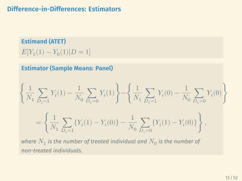
Estimand (ATET)𝐸[𝑌1(1) − 𝑌0(1)|𝐷 = 1]
Estimator (Sample Means: Panel)
{ 1𝑁1
∑𝐷𝑖=1
𝑌𝑖(1) − 1𝑁0
∑𝐷𝑖=0
𝑌𝑖(1)}−{ 1𝑁1
∑𝐷𝑖=1
𝑌𝑖(0) − 1𝑁0
∑𝐷𝑖=0
𝑌𝑖(0)}
= { 1𝑁1
∑𝐷𝑖=1
{𝑌𝑖(1) − 𝑌𝑖(0)} − 1𝑁0
∑𝐷𝑖=0
{𝑌𝑖(1) − 𝑌𝑖(0)}} ,
where 𝑁1 is the number of treated individual and 𝑁0 is the number ofnon-treated individuals.
13 / 52
Example
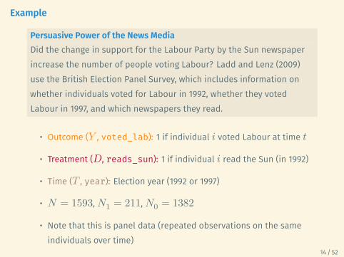
Persuasive Power of the News MediaDid the change in support for the Labour Party by the Sun newspaperincrease the number of people voting Labour? Ladd and Lenz (2009)use the British Election Panel Survey, which includes information onwhether individuals voted for Labour in 1992, whether they votedLabour in 1997, and which newspapers they read.
• Outcome (𝑌 , voted_lab): 1 if individual 𝑖 voted Labour at time 𝑡
• Treatment (𝐷, reads_sun): 1 if individual 𝑖 read the Sun (in 1992)
• Time (𝑇 , year): Election year (1992 or 1997)
• 𝑁 = 1593, 𝑁1 = 211, 𝑁0 = 1382
• Note that this is panel data (repeated observations on the sameindividuals over time)
14 / 52
Example
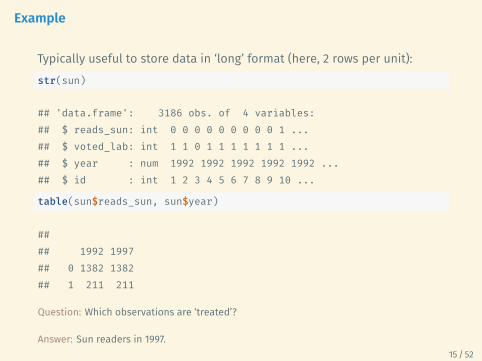
Typically useful to store data in ‘long’ format (here, 2 rows per unit):str(sun)
## 'data.frame': 3186 obs. of 4 variables:## $ reads_sun: int 0 0 0 0 0 0 0 0 0 1 ...## $ voted_lab: int 1 1 0 1 1 1 1 1 1 1 ...## $ year : num 1992 1992 1992 1992 1992 ...## $ id : int 1 2 3 4 5 6 7 8 9 10 ...
table(sun$reads_sun, sun$year)
#### 1992 1997## 0 1382 1382## 1 211 211
Question: Which observations are ‘treated’?
Answer: Sun readers in 1997.15 / 52
Example
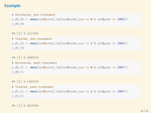
# Untreated, pre-treatmenty_d0_t0 <- mean(sun$voted_lab[sun$reads_sun == 0 & sun$year == 1992])y_d0_t0
## [1] 0.3227207# Treated, pre-treatmenty_d1_t0 <- mean(sun$voted_lab[sun$reads_sun == 1 & sun$year == 1992])y_d1_t0
## [1] 0.3886256# Untreated, post-treatmenty_d0_t1 <- mean(sun$voted_lab[sun$reads_sun == 0 & sun$year == 1997])y_d0_t1
## [1] 0.4305355# Treated, post-treatmenty_d1_t1 <- mean(sun$voted_lab[sun$reads_sun == 1 & sun$year == 1997])y_d1_t1
## [1] 0.582938416 / 52
Example
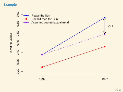
0.30
0.35
0.40
0.45
0.50
0.55
0.60
% v
otin
g La
bour
1992 1997
Reads the SunDoesn't read the SunAssumed counterfactual trend
ATT
17 / 52
Example
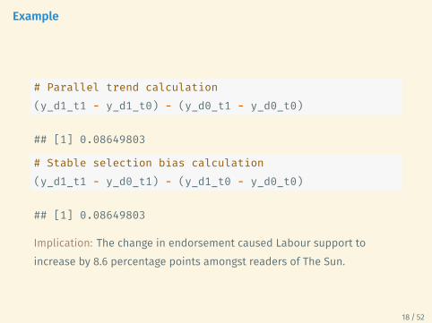
# Parallel trend calculation(y_d1_t1 - y_d1_t0) - (y_d0_t1 - y_d0_t0)
## [1] 0.08649803
# Stable selection bias calculation(y_d1_t1 - y_d0_t1) - (y_d1_t0 - y_d0_t0)
## [1] 0.08649803
Implication: The change in endorsement caused Labour support toincrease by 8.6 percentage points amongst readers of The Sun.
18 / 52
Regression DD
Difference-in-Differences: Regression Estimator
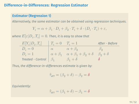
Estimator (Regression 1)Alternatively, the same estimator can be obtained using regression techniques.
𝑌𝑖 = 𝛼 + 𝛽1 ⋅ 𝐷𝑖 + 𝛽2 ⋅ 𝑇𝑖 + 𝛿 ⋅ (𝐷𝑖 ⋅ 𝑇𝑖) + 𝜀,where 𝐸[𝜀|𝐷𝑖, 𝑇𝑖] = 0. Then, it is easy to show that
𝐸[𝑌𝑖|𝐷𝑖, 𝑇𝑖] 𝑇𝑖 = 0 𝑇𝑖 = 1 After - Before𝐷𝑖 = 0 𝛼 𝛼 + 𝛽2 𝛽2𝐷𝑖 = 1 𝛼 + 𝛽1 𝛼 + 𝛽1 + 𝛽2 + 𝛿 𝛽2 + 𝛿Treated - Control 𝛽1 𝛽1 + 𝛿 𝛿
Thus, the difference-in-differences estimate is given by:
𝜏ATT = (𝛽2 + 𝛿) − 𝛽2 = 𝛿
Equivalently:𝜏ATT = (𝛽1 + 𝛿) − 𝛽1 = 𝛿
19 / 52
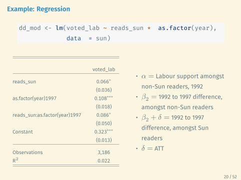
Example: Regression
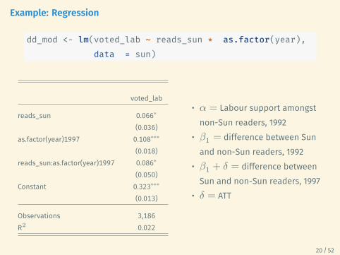
dd_mod <- lm(voted_lab ~ reads_sun * as.factor(year),data = sun)
voted_lab
reads_sun 0.066∗
(0.036)as.factor(year)1997 0.108∗∗∗
(0.018)reads_sun:as.factor(year)1997 0.086∗
(0.050)Constant 0.323∗∗∗
(0.013)
Observations 3,186R2 0.022
• 𝛼 = Labour support amongstnon-Sun readers, 1992
• 𝛽1 = difference between Sunand non-Sun readers, 1992
• 𝛽1 + 𝛿 = difference betweenSun and non-Sun readers, 1997
• 𝛿 = ATT
20 / 52
Example: Regression
dd_mod <- lm(voted_lab ~ reads_sun * as.factor(year),data = sun)
voted_lab
reads_sun 0.066∗
(0.036)as.factor(year)1997 0.108∗∗∗
(0.018)reads_sun:as.factor(year)1997 0.086∗
(0.050)Constant 0.323∗∗∗
(0.013)
Observations 3,186R2 0.022
• 𝛼 = Labour support amongstnon-Sun readers, 1992
• 𝛽2 = 1992 to 1997 difference,amongst non-Sun readers
• 𝛽2 + 𝛿 = 1992 to 1997difference, amongst Sunreaders
• 𝛿 = ATT
20 / 52
Cross-sectional regression estimator
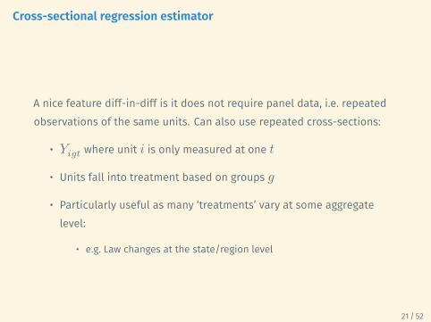
A nice feature diff-in-diff is it does not require panel data, i.e. repeatedobservations of the same units. Can also use repeated cross-sections:
• 𝑌𝑖𝑔𝑡 where unit 𝑖 is only measured at one 𝑡
• Units fall into treatment based on groups 𝑔
• Particularly useful as many ‘treatments’ vary at some aggregatelevel:
• e.g. Law changes at the state/region level
21 / 52
Cross-sectional regression estimator
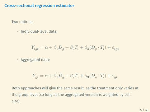
Two options:
• Individual-level data:
𝑌𝑖𝑔𝑡 = 𝛼 + 𝛽1𝐷𝑔 + 𝛽2𝑇𝑖 + 𝛽3(𝐷𝑔 ⋅ 𝑇𝑖) + 𝜀𝑖𝑔𝑡
• Aggregated data:
𝑌𝑔𝑡 = 𝛼 + 𝛽1𝐷𝑔 + 𝛽2𝑇𝑖 + 𝛽3(𝐷𝑔 ⋅ 𝑇𝑖) + 𝜀𝑔𝑡
Both approaches will give the same result, as the treatment only varies atthe group level (so long as the aggregated version is weighted by cellsize).
22 / 52
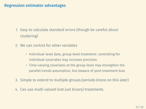
Regression estimator advantages
1. Easy to calculate standard errors (though be careful aboutclustering)
2. We can control for other variables
• Individual-level data, group-level treatment: controlling forindividual covariates may increase precision
• Time-varying covariates at the group-level may strengthen theparallel trends assumption, but beware of post-treatment bias
3. Simple to extend to multiple groups/periods (more on this later)
4. Can use multi-valued (not just binary) treatments
23 / 52
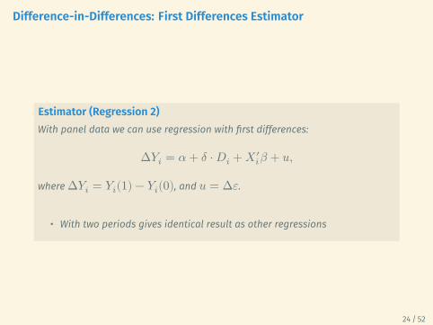
Difference-in-Differences: First Differences Estimator
Estimator (Regression 2)With panel data we can use regression with first differences:
Δ𝑌𝑖 = 𝛼 + 𝛿 ⋅ 𝐷𝑖 + 𝑋′𝑖𝛽 + 𝑢,
where Δ𝑌𝑖 = 𝑌𝑖(1) − 𝑌𝑖(0), and 𝑢 = Δ𝜀.
• With two periods gives identical result as other regressions
24 / 52
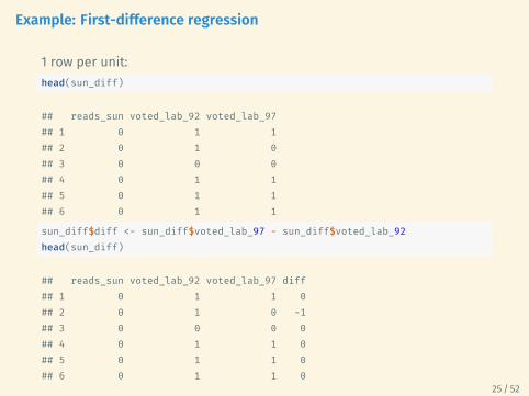
Example: First-difference regression
1 row per unit:head(sun_diff)
## reads_sun voted_lab_92 voted_lab_97## 1 0 1 1## 2 0 1 0## 3 0 0 0## 4 0 1 1## 5 0 1 1## 6 0 1 1
sun_diff$diff <- sun_diff$voted_lab_97 - sun_diff$voted_lab_92head(sun_diff)
## reads_sun voted_lab_92 voted_lab_97 diff## 1 0 1 1 0## 2 0 1 0 -1## 3 0 0 0 0## 4 0 1 1 0## 5 0 1 1 0## 6 0 1 1 0
25 / 52
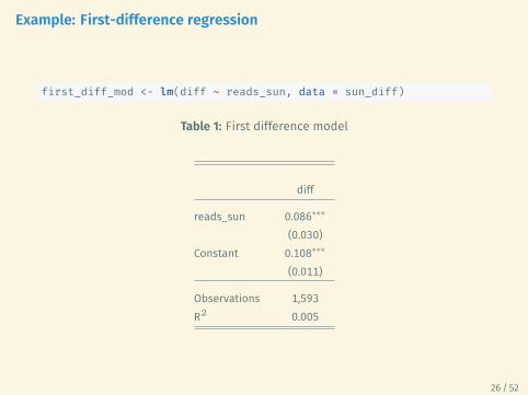
Example: First-difference regression
first_diff_mod <- lm(diff ~ reads_sun, data = sun_diff)
Table 1: First difference model
diff
reads_sun 0.086∗∗∗
(0.030)Constant 0.108∗∗∗
(0.011)
Observations 1,593R2 0.005
26 / 52

Break
27 / 52

Threats to Validity

Non-parallel trends
Critical identification assumption: treatment units have similar trends tocontrol units in the absence of treatment.
Question: Why is this assumption untestable?
Answer: because of the FPOCI → we cannot observe potential outcomeunder the control condition for treated units in the post-treatmentperiod.
28 / 52
Potential violations of parallel trends
• “Ashenfelter’s Dip”
• Participants in worker training programs may experience decreasedearnings before they enter the program (why are they participating?)
• If wages revert to the mean, comparing wages of participants andnon-participants leads to an upwardly biased estimate
• Targeting
• Policymakers may target units who are most improving
29 / 52
Assessing (non-)parallel trends
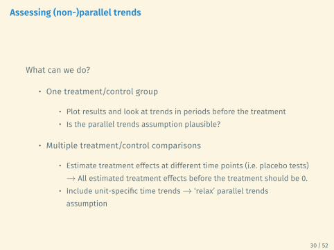
What can we do?
• One treatment/control group
• Plot results and look at trends in periods before the treatment• Is the parallel trends assumption plausible?
• Multiple treatment/control comparisons
• Estimate treatment effects at different time points (i.e. placebo tests)→ All estimated treatment effects before the treatment should be 0.
• Include unit-specific time trends → ‘relax’ parallel trendsassumption
30 / 52
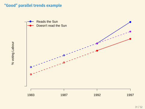
“Good” parallel trends example%
vot
ing
Labo
ur
1983 1987 1992 1997
Reads the SunDoesn't read the Sun
31 / 52
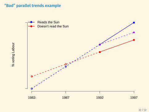
“Bad” parallel trends example%
vot
ing
Labo
ur
1983 1987 1992 1997
Reads the SunDoesn't read the Sun
32 / 52
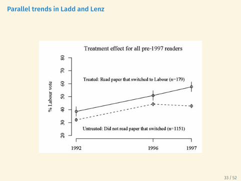
Parallel trends in Ladd and Lenz
33 / 52
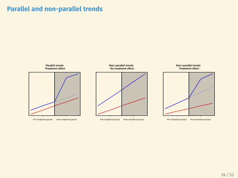
Parallel and non-parallel trends
Parallel trends Treatment effect
Pre−treatment period Post−treatment period
Non−parallel trends No treatment effect
Pre−treatment period Post−treatment period
Non−parallel trends Treatment effect
Pre−treatment period Post−treatment period
34 / 52

Multiple periods
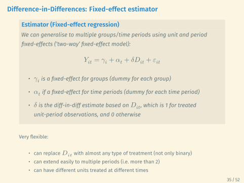
Difference-in-Differences: Fixed-effect estimator
Estimator (Fixed-effect regression)We can generalise to multiple groups/time periods using unit and periodfixed-effects (‘two-way’ fixed-effect model):
𝑌𝑖𝑡 = 𝛾𝑖 + 𝛼𝑡 + 𝛿𝐷𝑖𝑡 + 𝜀𝑖𝑡
• 𝛾𝑖 is a fixed-effect for groups (dummy for each group)
• 𝛼𝑡 if a fixed-effect for time periods (dummy for each time period)
• 𝛿 is the diff-in-diff estimate based on 𝐷𝑖𝑡, which is 1 for treatedunit-period observations, and 0 otherwise
Very flexible:
• can replace 𝐷𝑖𝑡 with almost any type of treatment (not only binary)• can extend easily to multiple periods (i.e. more than 2)• can have different units treated at different times
35 / 52
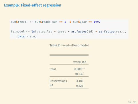
Example: Fixed-effect regression
sun$treat <- sun$reads_sun == 1 & sun$year == 1997
fe_model <- lm(voted_lab ~ treat + as.factor(id) + as.factor(year),data = sun)
Table 2: Fixed-effect model
voted_lab
treat 0.086∗∗∗
(0.030)
Observations 3,186R2 0.826
36 / 52
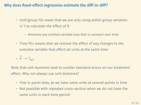
Why does fixed-effect regression estimate the diff-in-diff?
• Unit/group FEs mean that we are only using within group variationin Y to calculate the effect of D
• Removes any omitted variable bias that is constant over time
• Time FEs means that we remove the effect of any changes to theoutcome variable that affect all units at the same time
• 𝛿 → 𝜏ATTNote that unit dummies lead to smaller standard errors on our treatmenteffect. Why not always use unit dummies?
• Fine in panel data, as we have same units at several points in time• Not possible with repeated cross-section when we do not have thesame units in each time period
37 / 52
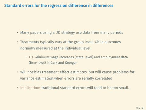
Standard errors for the regression difference in differences
• Many papers using a DD strategy use data from many periods
• Treatments typically vary at the group level, while outcomesnormally measured at the individual level
• E.g. Minimum wage increases (state-level) and employment data(firm-level) in Cark and Krueger
• Will not bias treatment effect estimates, but will cause problems forvariance estimation when errors are serially correlated
• Implication: traditional standard errors will tend to be too small.
38 / 52
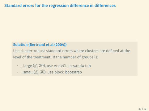
Standard errors for the regression difference in differences
Solution (Bertrand et al (2004))Use cluster-robust standard errors where clusters are defined at thelevel of the treatment. If the number of groups is:
• …large (⪆ 30), use vcovCL in sandwich• …small (⪅ 30), use block-bootstrap
39 / 52

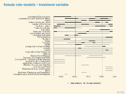
Example: Multiperiod diff-in-diff
Female role-models in politicsWhen women are promoted to high-office, do they motivate otherwomen to participate more in policymaking? Blumenau (2019) examinesthe participation of female MPs in parliamentary debates between 1997and 2018 as a proxy for policymaking involvement. If high-profilewomen act as role-models, when they are promoted they shouldencourage other women to participate more.
• Outcome (𝑌 , prop_words): Proportion of words spoken by women in debate 𝑑 atin ministry 𝑚 at time 𝑡
• Treatment (𝐷, female_minister): 1 if cabinet minister of ministry 𝑚 at time 𝑡 isfemale
• Unit of analysis: Debates (clustered within about 30 ministries)
• 𝑁 ≈ 15,000 debates
• Time measured at the month level (i.e. February 2012, etc)
40 / 52
Female role-models – treatment variable
41 / 52
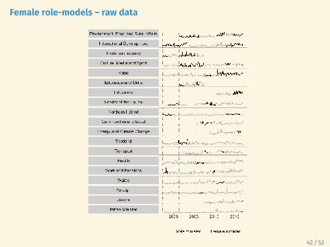
Female role-models – raw data
42 / 52
Female role-models – model specification
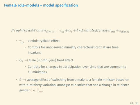
𝑃𝑟𝑜𝑝𝑊𝑜𝑟𝑑𝑠𝑊𝑜𝑚𝑒𝑛𝑑(𝑚𝑡) = 𝛾𝑚 +𝛼𝑡 +𝛿 ∗𝐹𝑒𝑚𝑎𝑙𝑒𝑀𝑖𝑛𝑖𝑠𝑡𝑒𝑟𝑚𝑡 +𝜀𝑑(𝑚𝑡)
• 𝛾𝑚 → ministry fixed effect
• Controls for unobserved ministry characteristics that are timeinvariant
• 𝛼𝑡 → time (month-year) fixed effect
• Controls for changes in participation over time that are common toall ministries
• 𝛿 → average effect of switching from a male to a female minister based onwithin-ministry variation, amongst ministries that see a change in ministergender (i.e. 𝜏ATT)
43 / 52
R example
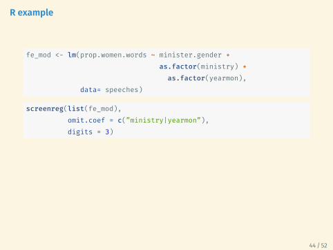
fe_mod <- lm(prop.women.words ~ minister.gender +as.factor(ministry) +
as.factor(yearmon),data= speeches)
screenreg(list(fe_mod),omit.coef = c(”ministry|yearmon”),digits = 3)
44 / 52
R example
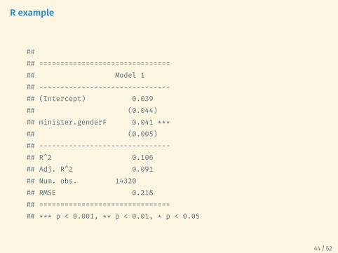
#### ===============================## Model 1## -------------------------------## (Intercept) 0.039## (0.044)## minister.genderF 0.041 ***## (0.005)## -------------------------------## R^2 0.106## Adj. R^2 0.091## Num. obs. 14320## RMSE 0.218## ===============================## *** p < 0.001, ** p < 0.01, * p < 0.05
44 / 52
R example (clustered errors)
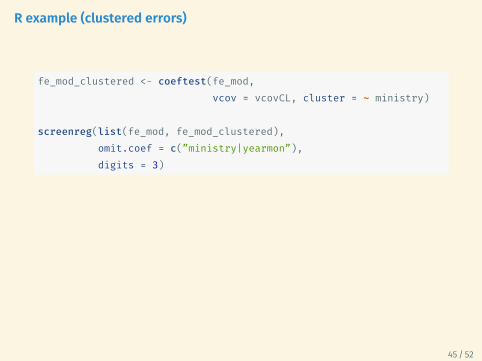
fe_mod_clustered <- coeftest(fe_mod,vcov = vcovCL, cluster = ~ ministry)
screenreg(list(fe_mod, fe_mod_clustered),omit.coef = c(”ministry|yearmon”),digits = 3)
45 / 52
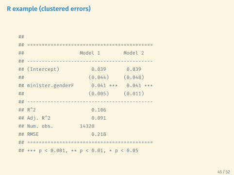
R example (clustered errors)
#### ===========================================## Model 1 Model 2## -------------------------------------------## (Intercept) 0.039 0.039## (0.044) (0.048)## minister.genderF 0.041 *** 0.041 ***## (0.005) (0.011)## -------------------------------------------## R^2 0.106## Adj. R^2 0.091## Num. obs. 14320## RMSE 0.218## ===========================================## *** p < 0.001, ** p < 0.01, * p < 0.05
45 / 52
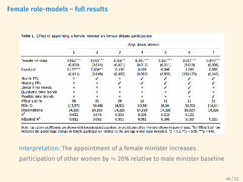
Female role-models – full results
Interpretation: The appointment of a female minister increasesparticipation of other women by≈ 20% relative to male minister baseline
46 / 52
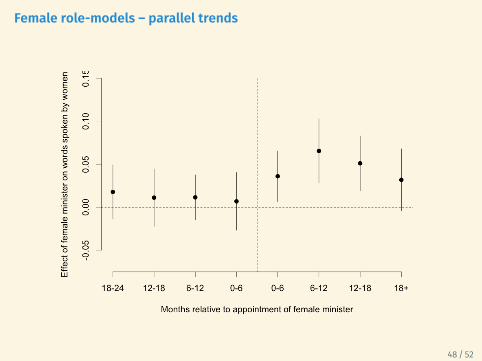
Female role-models – parallel trends
Hard to provide a visual inspection of the parallel trends assumption astreatment switches on and off over time in different ministries.
Nevertheless, we are still assuming that treated/control ministries wouldhave evolved identically over time in absense of treatment.
One way forward, test for 𝑚 “lags” and 𝑞 “leads” of the treatment:
𝑦𝑑(𝑚𝑡) = 𝛼0 +𝑚
∑𝑗=−𝑞
𝛿𝑗 ∗𝐹𝑒𝑚𝑎𝑙𝑒𝑀𝑖𝑛𝑖𝑠𝑡𝑒𝑟𝑚(𝑡+𝑗) +𝛾𝑚0 +𝛼𝑡 +𝜀𝑑(𝑚𝑡)
• 𝛿−1, 𝛿−2, ..., 𝛿−𝑞 are the “lead” effects which should all be 0
• 𝛿1, 𝛿2, ..., 𝛿𝑚 are the “lagged” effects which may take differentvalues
Intuition: What is the DD estimate in the Sun example using only datafrom 1992 and 1996? 47 / 52
Female role-models – parallel trends
48 / 52

Conclusion
Data requirements for Diff-in-diff
Data structure:
• Panel data or repeated cross-section• Single or multiple treatments• Continuous or binary treatments• Works both at individual/aggregate level
Does this require more data?
• Adding a time dimension can increase the amount of data you need• No need to control for extensive covariates (so long as they are fixedwithin units over time) which might mean decreased data collection
49 / 52

Examples of diff-in-diff designs
1. Card & Krueger, 1994• RQ: Do increases in the minimum wage reduce employment?• Outcome: Employment growth in fast-food restaurants• Treatment: Increased minimum wage in New Jersey; no change inPennsylvania
• Time: Before/after minimum wage changed
2. Dinas et al., 2019• RQ: What is the effect of refugee arrivals on support for the far right?• Outcome: Municipal support for far right party• Treatment: Refugee arrivals in Greek islands• Time: Elections before/after refugee crisis
50 / 52

Examples of diff-in-diff designs
3. Bechtel & Heinmueller, 2011• RQ: What is the effect of good policy on government support?• Outcome: Support for the German SPD in parliamentaryconstituencies
• Treatment: Flooded German regions close to the River Elbe• Time: Elections before/after 2002, when the Elbe flooded
4. Hainmueller & Hangartner, 2019• RQ: What is the effect of direct democracy on immigrantassimilation?
• Outcome: Naturalization rate of immigrants in Swiss municipalities• Treatment: Whether municipality decides on naturalisation requestsvia expert or citizen councils
• Time: Decisions before/after legal changes to decision making inmunicipalities
50 / 52
Conclusion
The DD design allows for a comparison over time in the treatment group,controlling for concurrent time trends using a control group.
DD requires data on multiple units in multiple periods, but can beapplied to panel data or repeated cross-sectional data.
DD is very widely used, as it is a powerful conditioning strategy thatdoesn’t require endless lists of covariates to strengthen the identifyingassumption.
The identification assumption – that treatment and control units wouldfollow parallel trends in the absense of treatment – should beinvestigated with every application!
51 / 52
After reading week
Synthetic control method
52 / 52
Recommended


![The effects of a redesign on students’ attitudes and ... · conceptual understanding regarding forces. Using the Hake gain [3], 𝑔= 𝑃𝑃𝑃𝑃−𝑃𝑃𝑃 100%−𝑃𝑃𝑃,](https://img.pdfslide.net/doc/110x75/5f0ad4d07e708231d42d8dec/the-effects-of-a-redesign-on-studentsa-attitudes-and-conceptual-understanding.jpg)