AFRL-IF-RS-TR-2004-101 Final Technical Report April 2004 QOS AND CONTROL-THEORETIC TECHNIQUES FOR INTRUSION TOLERANCE Arizona State University
APPROVED FOR PUBLIC RELEASE; DISTRIBUTION UNLIMITED.
AIR FORCE RESEARCH LABORATORY INFORMATION DIRECTORATE
ROME RESEARCH SITE ROME, NEW YORK

STINFO FINAL REPORT
This report has been reviewed by the Air Force Research Laboratory, Information Directorate, Public Affairs Office (IFOIPA) and is releasable to the National Technical Information Service (NTIS). At NTIS it will be releasable to the general public, including foreign nations. AFRL-IF-RS-TR-2004-101 has been reviewed and is approved for publication APPROVED: /s/ JOHN C. FAUST Project Engineer FOR THE DIRECTOR: /s/ WARREN H. DEBANY, JR. Technical Advisor Information Grid Division Information Directorate

REPORT DOCUMENTATION PAGE Form Approved
OMB No. 074-0188 Public reporting burden for this collection of information is estimated to average 1 hour per response, including the time for reviewing instructions, searching existing data sources, gathering and maintaining the data needed, and completing and reviewing this collection of information. Send comments regarding this burden estimate or any other aspect of this collection of information, including suggestions for reducing this burden to Washington Headquarters Services, Directorate for Information Operations and Reports, 1215 Jefferson Davis Highway, Suite 1204, Arlington, VA 22202-4302, and to the Office of Management and Budget, Paperwork Reduction Project (0704-0188), Washington, DC 20503 1. AGENCY USE ONLY (Leave blank)
2. REPORT DATEAPRIL 2004
3. REPORT TYPE AND DATES COVERED FINAL Apr 01 – Sep 02
4. TITLE AND SUBTITLE QOS AND CONTROL-THEORETIC TECHNIQUES FOR INTRUSION TOLERANCE
6. AUTHOR(S) Nong Ye
5. FUNDING NUMBERS G - F30602-01-1-0510 PE - 62702F PR - OIPG TA - 32 WU - P2
7. PERFORMING ORGANIZATION NAME(S) AND ADDRESS(ES) Arizona State University Box 875906 1711 S. Rural Road, Goldwater Center, Room 502 Tempe AZ 85287
8. PERFORMING ORGANIZATION REPORT NUMBER N/A
9. SPONSORING / MONITORING AGENCY NAME(S) AND ADDRESS(ES) AFRL/IFGB 525 Brooks Road Rome NY 13441-4505
10. SPONSORING / MONITORING AGENCY REPORT NUMBER AFRL-IF-RS-TR-2004-101
11. SUPPLEMENTARY NOTES AFRL Project Engineer: John C. Faust/IFGB/(315) 330-4544 John.Faust @rl.af.mil
12a. DISTRIBUTION / AVAILABILITY STATEMENT
APPROVED FOR PUBLIC RELEASE; DISTRIBUTION UNLIMITED.
12b. DISTRIBUTION CODE
13. ABSTRACT (Maximum 200 Words) As we increasingly rely on information systems to support a multitude of critical operations, it becomes more and more important that these systems are able to deliver Quality of Service (QoS), even in the face of intrusions. This report examines two host-based resources, a router and a web server, and presents simulated models of modifications that can be made to these resources to make them QoS-capable. Two different QoS models are investigated for the router. The first model implements a router with a feedback control loop that monitors the instantaneous QoS guarantee and adjusts the router’s admission control of new requests accordingly. The second router model, called Adjusted Weighted Shortest Processing Time, queues data packets according to a weight which is dependent on their initial priority weight and the amount of time they have awaited service. For the web server, six queuing disciplines are simulated and analyzed for their efficiency in delivering QoS. These disciplines are compared on the basis of selected QoS measurements, including lateness, drop rate, time-in-system and throughput. We find that there is not necessarily one best queuing rule to follow; the appropriate selection depends on the needs of that web server.
15. NUMBER OF PAGES14. SUBJECT TERMS Quality of Service, Router, Web Server, QoS-Aware Router, Adjusted Weighted Shortest Processing Time, QoS-Aware Web Server, Web Server Scheduling, Queuing Disciplines 16. PRICE CODE
17. SECURITY CLASSIFICATION OF REPORT
UNCLASSIFIED
18. SECURITY CLASSIFICATION OF THIS PAGE
UNCLASSIFIED
19. SECURITY CLASSIFICATION OF ABSTRACT
UNCLASSIFIED
20. LIMITATION OF ABSTRACT
UL
NSN 7540-01-280-5500 Standard Form 298 (Rev. 2-89) Prescribed by ANSI Std. Z39-18 298-102
80

Abstract As we increasingly rely on information systems to support a multitude of critical
operations, it becomes more and more important that these systems are able to deliver quality of service, even in the face of intrusions. One common class of cyber-attacks is the flooding of the system’s resources with requests for service. Thus, a reliable information system must be able to adeptly handle a large number of requests efficiently so that legitimate users may still use the system even as illegitimate users are attempting to flood the system.
This report examines two host-based resources and presents simulated models of modifications that can be made to these resources to make them capable of handling a number of requests. The two resources examined are a router and a web server.
There are two different quality of service models presented for the router. The first model implements a router with a feedback control loop that monitors the instantaneous quality of service guarantee and adjusts the router’s admission control of new requests accordingly. This model is compared to the basic router model that represents the typical configuration currently in use. The resulting comparison indicates that the feedback control loop is an improvement on the existing basic router. It decreases the time-in-system for data packets, and reduces packet loss, but does not fully utilize its bandwidth as well as a basic router with over-characterization.
The second router model suggests a new approach of queuing new requests for service. This approach is called Adjusted Weighted Shortest Processing Time and queues data packets according to a weight, which is dependent on their initial priority weight and the amount of time they have awaited service. The new approach is compared to two other queuing disciplines – Weighted Shortest Processing Time and First-Come First-Serve. We present data that indicate that the Adjusted Weighted Shortest Processing Time discipline improves the high time-in-system variance that exists in the Weighted Shortest Processing Time discipline, but it does not fairly allocate resources to both high and low priority data packets.
For the web server, six queuing disciplines are simulated and analyzed for their efficiency in delivering quality of service. These disciplines are Best Effort, Differentiated Services, Apparent Tardiness Cost, Earliest Due Date, Weighted Shortest Processing Time, and Weighted Only. These disciplines are compared on the basis of selected quality of service measurements, including lateness, drop rate, time-in-system, and throughput. We find that there is not necessarily one best queuing rule to follow; the appropriate discipline selection depends on the needs of that web server.

i
Table of Contents
INTRODUCTION ..................................................................................................1
CHAPTER 1: ROUTER QUALITY OF SERVICE MODEL WITH FEEDBACK CONTROL ............................................................................................................3
1-1 Router with Feedback Control Loop .................................................................. 3 1-1.1 Overview of Router Design ............................................................................ 4 1-1.2 Design Specification ....................................................................................... 6
1-2 Simulation and Experiment ................................................................................. 9 1-2.1 Simulation Models .......................................................................................... 9 1-2.2 Experiment.................................................................................................... 12
1-3 Results and Discussion........................................................................................ 18 1-3.1 Heavy Traffic Condition ............................................................................... 19 1-3.2 Light traffic condition ................................................................................... 20 1-3.3 Conclusions................................................................................................... 21
CHAPTER 2: ROUTER SERVICE DIFFERENTIATION BY ADJUSTED WEIGHTED SHORTEST PROCESSING TIME SERVICE DISCIPLINE ............23
2-1 A-WSPT Service Discipline................................................................................ 23
2-2 Simulations and Experiment.............................................................................. 27
2-3 Results and Discussion........................................................................................ 29 2-3.1 Heavy traffic ................................................................................................. 29 2-3.2 Light traffic ................................................................................................... 34 2-3.3 Conclusions................................................................................................... 38
CHAPTER 3: PROVIDING QUALITY OF SERVICE FOR A WEB SERVER USING QUEUING DISCIPLINES .......................................................................39
3-1 QoS Delivery for a Web Server ......................................................................... 39 3-1.1 Previous Approaches .................................................................................... 39 3-1.2 Web Server Operation................................................................................... 42 3-1.3 QoS Measures ............................................................................................... 44
3-2 Discussion of Different Queuing Disciplines..................................................... 45
3-3 Simulation of Different Queuing Rules............................................................. 48
3-4 Experimental Results.......................................................................................... 53 3-4.1 Heavy-traffic Case ........................................................................................ 53 3-4.2 Light-Traffic Case......................................................................................... 62
3-5 Conclusions.......................................................................................................... 69
REFERENCES ...................................................................................................72

ii
List of Figures
Figure 1-1. The basic router QoS model............................................................................. 6 Figure 1-2. The QoS model with feedback control............................................................. 7 Figure 1-3. Simulated router with “basic” QoS model. ...................................................... 9 Figure 1-4. Simulated router with “feedback” QoS model............................................... 11 Figure 1-5. Token rates with different proportional gain values. .................................... 15 Figure 1-6. Token rates with different integral gain values............................................. 16 Figure 1-7. Token rates with different differential gain values. ...................................... 17 Figure 1-8. Throughput of high priority traffic with different queue length upper bound............................................................................................................................................ 18 Figure 1-9. Time-in-system of feedback router and basic routers (heavy traffic). .......... 19 Figure 1-10. Throughput of feedback router and basic routers (heavy traffic) ................ 20 Figure 1-11. Time-in-system of feedback router and basic routers (light traffic). ........... 20 Figure 1-12. Throughput of feedback router and basic routers (light traffic)................... 21 Figure 2-1. Service order and the insertion of the packet. ................................................ 26 Figure 2-2. Router model in OPNET Modeler. ................................................................ 28 Figure 2-3. Time-in-system of high priority traffic (heavy traffic). ................................. 30 Figure 2-4. Time-in-system of low priority traffic (FCFS). ............................................. 31 Figure 2-5. Throughput of high priority traffic (heavy traffic)......................................... 33 Figure 2-6. Throughput of low priority traffic (heavy traffic).......................................... 33 Figure 2-7. Throughput of overall traffic (heavy traffic).................................................. 34 Figure 2-8. Time-in-system of high priority traffic (light traffic). ................................... 35 Figure 2-9. Time-in-system of low priority traffic (light traffic)...................................... 35 Figure 2-10. Throughput of high priority traffic (light traffic). ........................................ 36 Figure 2-11. Throughput of low priority traffic (light traffic). ......................................... 37 Figure 2-12. Throughput of all traffic (light traffic). ........................................................ 37 Figure 3-1. Web server QoS model. ................................................................................ 43 Figure 3-2. Basic DiffServ queuing rule model................................................................ 46 Figure 3-3. The topology of the QoS web server simulation........................................... 48 Figure 3-4. Overall time-in-system in the heavy-traffic scenario.................................... 53 Figure 3-5. Queue size in the heavy-traffic scenario. ...................................................... 54 Figure 3-6. Time-in-system of Class 4 in the heavy-traffic scenario. ............................. 55 Figure 3-7. Time-in-system of Class 2 in the heavy traffic scenario................................ 56 Figure 3-8. Time-in-system of Class 1 in the heavy traffic scenario............................... 56 Figure 3-9. Overall drop in the heavy traffic scenario..................................................... 57 Figure 3-10. Drop of Class 4 in overwhelming scenario. ................................................ 57 Figure 3-11. Drop of Class 2 in overwhelming scenario. ................................................. 58 Figure 3-12. Drop of Class 1 in overwhelming scenario. ................................................. 59 Figure 3-13. Overall time-in-system in light-traffic scenario........................................... 63 Figure 3-14. Queue size in light-traffic scenario. ............................................................ 63 Figure 3-15. Time-in-system of Class 4 in light-traffic scenario..................................... 64 Figure 3-16. Time-in-system of Class 2 in light-traffic scenario..................................... 65

iii
Figure 3-17. Time-in-system of Class 1 in light-traffic scenario...................................... 65 Figure 3-18. Overall drop in light-traffic scenario........................................................... 66 Figure 3-19. Drop of Class 1 in light-traffic scenario...................................................... 66 Figure 3-20. Overall time-in-system of ATC with different scaling parameters............. 70
List of Tables
Table 1-1. Conditions for the simulation of heavy traffic. ............................................... 12 Table 1-2. Conditions for simulation of light traffic......................................................... 13 Table 1-3. The configurations of the basic router and feedback router. .......................... 13 Table 2-1. Packet loss for FCFS, WSPT, and A-WSPT disciplines under heavy traffic. 31 Table 3-1. Parameter settings in overwhelming scenario. ............................................... 50 Table 3-2. Time-in-system in heavy-traffic scenario: mean and deviation values. ......... 54 Table 3-3. Drop in heavy-traffic scenario........................................................................ 59 Table 3-4. Lateness in heavy-traffic scenario. ................................................................. 60 Table 3-5. Throughput in heavy-traffic scenario. ............................................................ 61 Table 3-6. Average queue size for heavy-traffic scenario. .............................................. 62 Table 3-7. Parameter settings in light-traffic scenario..................................................... 62 Table 3-8. Time-in-system in light-traffic scenario.......................................................... 63 Table 3-9. Drop in light-traffic scenario. ......................................................................... 66 Table 3-10. Lateness in light-traffic scenario. ................................................................. 67 Table 3-11. Throughput in light-traffic scenario. ............................................................ 68 Table 3-12. Average queue size in light-traffic scenario. ................................................. 69

1
Introduction Over the last decade, there has been an explosion in the usage of the Internet and
other information systems for personal and official purposes. As we increasingly rely on
information systems to support critical operations in defense, banking,
telecommunication, transportation, electric power and many other systems, intrusions
into these systems have become a significant threat to our society with potentially severe
consequences [1-2]. Therefore, it becomes increasingly important that these systems are
designed with a level of intrusion tolerance that enable them to continue functioning
correctly and providing services in a timely manner even in the face of intrusions, that is,
to maintain the quality of service (QoS) regardless of what intrusions occur.
Currently, information systems are designed using the “best-effort” model, in
which their resources are available to use regardless of their state. This model leaves the
system vulnerable to a depletion of its resources if it is sent a large number of service
requests from malicious users, which will effectively deny the availability of resources to
legitimate users. For example, massive amounts of data packets can be directed to a web
server at a site, thereby making the web server unavailable to take legitimate service
requests. Especially for mission-critical purposes, information systems must adopt a
robust design to resist such malicious exploits and to provide quality of service (QoS)
guarantees even in the face of intrusions.
The project described herein is the first part of a research project that will
establish the QoS-centric model of stateful resource management for building intrusion-
tolerant information systems. Unlike most existing efforts, which focus mostly on QoS of
network resources, such as ATM networks and multimedia communication over
communication channels, this project is focused on the QoS of host-based resources.
Since host-based resources are involved in all applications, their QoS management is
critical to the effectiveness of intrusion-tolerant information systems. The goal of this
project is to develop a control-theoretic approach to intrusion tolerance from a QoS-
centric resource management perspective in order to enable an information system to
continue its correct functioning and maintain QoS in the face of intrusions.

2
The research described within fulfills the requirements of the first phase of this
project. In this phase, we focused on two host-based resources – a router and a web server
– which we then analyzed and used to establish and demonstrate the feasibility of the
QoS and control-theoretic techniques. For each of these resources, we determined and
analyzed the characteristics of processes requesting services from the resource, and
defined the QoS metrics of the output performance of processes accordingly. We then
selected reliable control trigger techniques to monitor and detect changes in these metrics
and tested their performance in detecting intrusions. The next step was to develop
probes and tests that reveal the state of the resources when significant changes in the QoS
metrics of processes are detected, and test their performance in diagnosing the impact of
intrusions on the state of the resources. We used these results to develop control
mechanisms for the resources and then tested their performance in configuring resources
and scheduling processes to maintain QoS even under the impact of intrusions. Finally,
we implemented a prototype of the control loop integrating the reliable control trigger
techniques and the robust control mechanisms, and tested the integration prototype for its
overall performance of intrusion tolerance.
For the router, two control mechanisms were developed and analyzed. The first
mechanism is one that utilizes a feedback control loop that is capable of monitoring the
instantaneous QoS guarantee and adapting the admission control to reflect the router’s
resource availability. This model is described in detail in Chapter 1. The second
mechanism for the router is the modification of its service discipline. This new service
discipline queues packets according to their weight, adjusting a packet’s weight based on
the amount of time it has been waiting in the queue. In the event of congestion, lower
priority packets are simply dropped. This mechanism is described in more detail in
Chapter 2.
For the web server, we analyzed its performance under different queuing rules in
an attempt to find the rule that would maximize the QoS of the server. Six queuing rules
were analyzed, including the “best-effort” model currently employed to compare QoS of
the new models to the existing one. The details of these rules and the results of these
tests are described in Chapter 3.

3
Chapter 1: Router Quality of Service Model with Feedback Control
1-1 Router with Feedback Control Loop
One definition of QoS provided by Geoff Huston is “the ability to differentiate between
traffic or service types so that the network can treat one or more classes of traffic
differently than other types” [2]. According to this definition, QoS roots in the ability to
provide differentiated services with regards to different service requirements.
Currently, a typical router operates using one of two QoS architectures – either
Integrated Service (InteServ) or DiffServ. The difference between these two models is
that InteServ delivers QoS on a per-flow basis, while DiffServ delivers QoS on a per-
aggregate basis. In this context, flow is defined as “a distinguishable stream of related
datagrams that results from a single user activity and requires the same QoS” [3], and
aggregate is a superset of flow. An end-to-end bandwidth reservation is required to
guarantee the bandwidth to individual flow.
The InteServ model is made up of predictive service, best effort service and link-
sharing service. A reference framework is proposed for its implementation, under which
are packet scheduling, packet classification, admission control, and path reservation. The
per-flow based service differentiation provides a fine granularity to isolate flows from
each other, and thus, achieve firm end-to-end service guarantees. However, flow-based
technology is vulnerable to the scalability problem, especially in backbone networks,
where there are millions of flows and the management overhead is extremely high.
Differentiated Service (DiffServ) [4], which provides its QoS guarantee on a per-
aggregate basis, divides the network into domains. At the edge of the domain, traffic is
classified into aggregates, policed and marked in accordance to given administrative
policies. The core routers sitting inside the domain provide per-hop behavior (PHB)
corresponding to the traffic aggregate. Compared to InteServ, DiffServ needs no end-to-
end path reservation, pushing the complexity to the network edge. The coarser granularity

4
scales down the number of entities in the router, but it results in a weaker service
guarantee compared to that of the per-flow based approach.
Due to the variable nature of network traffic, the characterization of performance
requirements for traffic presents a significant challenge to providing QoS guarantees. Jim
Kurose [5] writes about four classes of approach to providing a QoS guarantee. Some
approaches – such as tightly controlled approaches – prevent a change in the traffic
characterization. Others – such as approximate approaches, bounding approaches, and
observation-based approaches – tolerate the change by taking into consideration the
change in the peak rate. Tightly controlled approaches condition the traffic with a non-
work conserving queuing discipline. To maintain consistent traffic characterization, the
tightly controlled approaches may purposely block the arriving session while allowing
the output link to be idle, causing potential low utilization of the output link. The other
approaches all require some sort of traffic characterization, but their characterizations are
approximate based on estimation or prediction. This inevitably leads to inaccuracies in
the traffic characterization, which in turn leads to inappropriate deliveries of QoS. In
both these approaches and tightly controlled approaches, there is always the possibility
that the actual incoming traffic either overuses or underutilizes allocated resource.
Overuse may result in delay increase and packet loss, which downgrades the QoS
guarantee. Under-use results in the waste of service capacity. This suggests that a new
approach is needed.
1-1.1 Overview of Router Design
The router model proposed in this chapter circumvents the question of how to
accurately characterize traffic by not requiring accurate traffic characterization at all.
This QoS model employs a performance-centric approach for QoS guarantee while best
utilizing the available resource. In this approach, the router is able to monitor the
performance output of the QoS guarantee. The traffic characterization of admission
control may be varied to a significant degree as long as the router is able to guarantee the
QoS with the allocated resource. The admission control admits enough traffic to
maximize the utilization of allocated resource while satisfying the performance
requirement. To support this approach, the router needs to be aware of the instantaneous

5
performance of QoS guarantee, and admission control needs to dynamically vary the
traffic characterization. However, the QoS model of the average router lacks the
adaptability needed to implement the proposed approach. In these models, the router is
unaware of the instantaneous state of both the utilization of resources and how well the
guarantee is provided. Also, the admission control policy of the routers is fixed during
operation until it is manually changed. Thus, to implement our performance-centric
approach, we must design a feedback control loop.
The designed control loop is made up of performance monitoring, the feedback
controller, and adaptive admission control. The performance of the QoS guarantee is
closely monitored according to the two important performance metrics for a router:
timeliness and precision [6]. In the context of a router’s QoS, the timeliness is measured
by the packet delay. Knowing that the queuing delay is the only controllable delay
component in the scope of this study, we take the time-in-system of the packet’s wait in
the queue as the measure of timeliness. The precision of the router is measured by the
packet loss rate.
The router should guarantee the timeliness and precision to all admitted packets.
If the router is running out of its service capacity, the packets are denied service upon
arrival to avoid deteriorating either the timeliness or packet loss of the router. Admission
control is customized with the ability to dynamically characterize the incoming traffic,
and traffic is admitted against this dynamic traffic profile. A feedback controller parses
the performance output, calculates the adjustment to the traffic characterization, and
feeds the adjustment to the admission control for actuation.
The design of the performance-centric QoS model is carried out in two steps.
First, we design a basic QoS model, which is capable of basic service differentiation,
resource allocation and fixed rate admission control. Then, we introduce a feedback
control loop to realize the performance-centric QoS guarantee.

6
1-1.2 Design Specification
Figure 1-1. The basic router QoS model
Before the feedback control loop can be applied to implement the performance-
centric QoS guarantee approach, a QoS model capable of basic service differentiation and
resource allocation is designed, as shown in Figure 1-1. The basic QoS model provides
two classes of service – high priority service and low priority service. The high priority
service is the traffic with timeliness and precision requirements. The low priority service
accommodates applications tolerable to both delay and packet loss. Our primary interest
is to guarantee the QoS to the high priority traffic. To simplify the study, we assumed that
the packets of each type of service have been tagged before they arrive at the router,
eliminating the needs for packet classification and marking. At each input port, the
admission control characterizes and conditions the high priority traffic using the token
bucket model. In the token-bucket model, allowed traffic is characterized by two
parameters – token rate r and bucket depth p. r dictates the long-term rate of admitted
traffic, and p specifies the maximum burst size of admitted traffic. The packets beyond
the allowed traffic characterization are discarded immediately upon arrival. An in-depth
discussion and introduction of the token bucket model are covered in Parekh and
Gallager’s work [7]. At each output port of the router, the packets are accepted into a
queuing buffer and scheduled for transmission with a priority queuing discipline. The
priority queue discipline enforces the bandwidth allocation between two classes of
service based on priority. Two queues, a high priority queue and a low priority queue, are
provided to contain the packets. The high priority queue and low priority queue are
dedicated to serve exclusively the high priority traffic and the low priority traffic
7
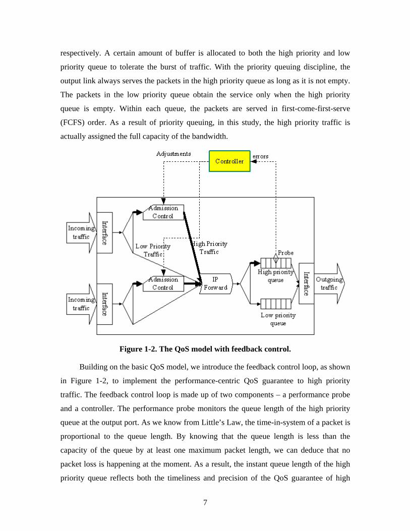
respectively. A certain amount of buffer is allocated to both the high priority and low
priority queue to tolerate the burst of traffic. With the priority queuing discipline, the
output link always serves the packets in the high priority queue as long as it is not empty.
The packets in the low priority queue obtain the service only when the high priority
queue is empty. Within each queue, the packets are served in first-come-first-serve
(FCFS) order. As a result of priority queuing, in this study, the high priority traffic is
actually assigned the full capacity of the bandwidth.
Figure 1-2. The QoS model with feedback control.
Building on the basic QoS model, we introduce the feedback control loop, as shown
in Figure 1-2, to implement the performance-centric QoS guarantee to high priority
traffic. The feedback control loop is made up of two components – a performance probe
and a controller. The performance probe monitors the queue length of the high priority
queue at the output port. As we know from Little’s Law, the time-in-system of a packet is
proportional to the queue length. By knowing that the queue length is less than the
capacity of the queue by at least one maximum packet length, we can deduce that no
packet loss is happening at the moment. As a result, the instant queue length of the high
priority queue reflects both the timeliness and precision of the QoS guarantee of high

8
priority traffic. The time-in-system can be bounded and the packet loss can be prevented
by bounding the queue length. An upper bound is set for the high priority queue length.
The error e is calculated from equation
Sle −= (1-1)
where l is the actual queue length of queue at the moment and S is the upper bound of the
queue length. A Proportional-Integral-Differential (PID) controller [8] constantly reads
the error e and calculates the adjustment µ with the PID equation
dtdeKedtKeK dip ++= ∫µ (1-2)
where Kp, Ki and Kd are proportional gain, integral gain and differential gain respectively,
and are all non-negative constants.
The adjustment for the rate of admission of packets is fed to the admission control
at each input port either to scale up or to scale down the admission rate of traffic. To
achieve fair admission control, the admission rate adjustment is split up among input
ports in proportion to the actual rate of incoming high priority traffic at each input port.
The input port contributing the most to the increase of queue length receives the largest
adjustment to its admission rate. For example, in case of a router with only two input
port, the total adjustment is split up between two input ports using equations
yx µµµ += (1-3)
and
*
*
YX
y
x =µµ
(1-4)
where µx, µy are the adjustments allocated for the two input ports respectively, and X*, Y*
are the actual rate of incoming high priority traffic at the two input ports respectively.
The divided adjustment is applied to bring down the token rate ri of the token bucket at
the corresponding input port for µi units, that is
iii rr µ−=' (1-5)
where ri and ri’ stand for the token rate of input port i at current moment and next
moment respectively, and i ∈ {all input ports}. By adjusting the token rate r, admission
control is able to scale up and down the amount of traffic actually admitted. When the

9
actual queue length exceeds the upper bound, the PID controller decreases the token rate
to slow down the incoming traffic, tending to bring the actual queue length back to within
upper bound.
1-2 Simulation and Experiment
To examine performance of the QoS guarantee with feedback control, the router QoS
model with feedback control (“feedback” model hereafter) and the basic router QoS
model without feedback control (“basic” model hereafter) are simulated and compared.
The simulation and experiment are accomplished in OPNET Modeler of OPNET
Technologies, Inc.
1-2.1 Simulation Models
Figure 1-3. Simulated router with “basic” QoS model.
The simulated router of the “basic” QoS model, shown in Figure 1-3, is composed
of two input ports, port 0 and 1, and only one output port, with an IP forwarder module

10
simulating the function of forwarding the packets from input ports to output port. Each
input port is associated with three traffic sources. In this study, we assume that all packets
come from either one of two input ports and go to the only output port. A priority based
queuing system is modeled at the output port. The queuing system is made up of a high
priority queue and a low priority queue with limited capacity, and uses a priority queuing
discipline. A packet sink is connected with the queuing module to collect the output
packets. The token bucket of the admission control has a fixed token rate, which is
unchanged during the whole simulation.
Each traffic source generates a traffic stream with a certain QoS requirement. Two
types of traffic are considered in this simulation – high priority and low priority. The
priority of traffic is marked in the Type-of-Service (ToS) field of the IP header of
belonging packets. In this study, ToS is set to 7 to indicate high priority traffic, and 0 for
low priority traffic. Since it is a general practice to assume the random arrival process as
a Poisson process, we specify that the inter-arrival time of packets is exponentially
distributed. Similarly, the size of packets generated by each source assumes normal
distribution. The expectation of the rate (bits per second) of the incoming traffic
generated by each source can be estimated by the ratio of mean packet size and mean
inter-arrival time.

11
Figure 1-4. Simulated router with “feedback” QoS model.
The simulated router that utilizes the “feedback” QoS model (Figure 1-4) is
designed by adding to the “basic” router model an additional feedback control loop
composed of a queue length probe, a PID controller, and admission control. Ideally, the
probe should monitor the queue length continuously. Since the arrivals and departures of
packets at the queue are discrete events, the queue length may undergo extreme and
abrupt variation. In the simulation, to avoid the high frequency vibration of the token rate
and to maintain the relative stability of the admission policy, the queue length is sampled
with a 2s interval, which is selected intuitively. To better bind the queue length, the
maximum value of the queue length in the interval is taken as the sample value of that
interval. For each admission control, the token rate starts with an initial level R. The PID
equation is simplified as the equation
)/()2()( 1211 −−−− −+−+−+= kkkkkdkkkikp TTeeeKTTeKeKµ (6)
with the integral and differential terms replaced with rectangular integration and linear
approximation of differentiation respectively. In the above equation, ei stands for the

12
error at time Ti, and Ti-1 stands for the last measure moment previous to Ti. The
adjustment splitter takes the real time statistic measure of the actual admission rate of
high priority traffic from both input ports to allocate their adjustments.
1-2.2 Experiment
The experiments for all router models are carried out under both “heavy” and “light”
traffic conditions. The heavy traffic condition simulates overwhelming high priority
traffic, in which the rate exceeds the capacity of output link. All six traffic sources
generate packets with size normally distributed, with mean 10,000 b and variance 2,000
b. The setting of the six traffic sources and rates of generated traffic are shown in Table
1-1. Source 0, 1, 3, and 4 generate high priority traffic, and source 2 and 5 generate low
priority traffic. Each input port generates high priority traffic at an average rate of
350,000 b/s and low priority traffic at 150,000 b/s. The total high priority traffic is
generated at 700,000 b/s, which is above the bandwidth of the output link.
Table 1-1. Conditions for the simulation of heavy traffic.
Interarrival Time Source Priority
Probability
Distribution
Mean
Rate of
Generated
Traffic
0 High Exponential 0.04000 s 250,000 b/s
1 High Exponential 0.10000 s 100,000 b/s
2 Low Exponential 0.06667 s 150,000 b/s
3 High Exponential 0.04000 s 250,000 b/s
4 High Exponential 0.10000 s 100,000 b/s
5 Low Exponential 0.06667 s 150, 000 b/s

13
Table 1-2. Conditions for simulation of light traffic.
Interarrival Time Source Priority
Probability
Distribution
Mean
Rate of
Generated
Traffic
0 High Exponential 0.13333 s 75,000 b/s
1 High Exponential 0.13333 s 75,000 b/s
2 Low Exponential 0.06667 s 150,000 b/s
3 High Exponential 0.13333 s 75,000 b/s
4 High Exponential 0.13333 s 75,000 b/s
5 Low Exponential 0.06667 s 150,000 b/s
The configuration for the light traffic condition is summarized in Table 1-2. Each
input port generates high priority traffic at a rate of 150,000 b/s and low priority traffic at
rate of 150,000 b/s. Total high priority traffic generated by both input ports is 350,000
b/s, which is lower than the bandwidth of the output link.
As mentioned previously, our primary concern is the timeliness and precision of
the QoS guarantee to high priority traffic, and its utilization of allocated bandwidth. Thus,
we collect the data concerning the time-in-system and the packet loss rate of the high
priority queue. We also collect throughput, which is the output rate of traffic, to reflect
the utilization of the bandwidth.
Table 1-3. The configurations of the basic router and feedback router.
Basic Model
(Over-
characterization)
Basic Model
(Under-
characterization)
Feedback Model
Bandwidth of output link 640 000 b/s 640 000 b/s 640 000 b/s
High priority queue capacity 100 000 b 100 000 b 100 000 b

14
Upper bound of queue length - - 80 000 bits
Low priority queue capacity 450 000 b/s 450 000 b/s 450 000 b/s
Token rate (Port 0, 1) 450 000 b/s 250 000 b/s 400 000 b/s (initial)
Bucket depth (Port 0, 1) 100 000 b 100 000 b 100 000 b
Proportional gain (Kp) - - 1.0
Integral gain (Ki) - - 0.2
Differential gain (Kd) - - 0.2
Control step length - - 2 s
The experiment is designed to compare admission control schemas of the
feedback router, the basic router with over-characterization (“basic (over)”), and the basic
router with under-characterization (“basic (under)”). The configurations of the routers of
each schema are shown in Table 1-3. The over-characterization admission control
characterizes the traffic with a loose upper bound, allowing great variance in the rate of
incoming traffic. In the basic (over) model, the token rates at both input ports are set to
450,000 b/s, allowing most of the traffic to enter the router. The under-characterization
admission control characterizes the traffic with a stringent bound. The basic (under)
model sets the token rates at both input ports to 250,000, which is lower than the average
rate of incoming traffic, with all other settings exactly the same as basic (over) model.
To make the feedback router comparable to the basic routers, it shares the same
setting as the basic models, except that it has a feedback control loop and variable token
rates for both admission controls. The proportional, integral and differential gains Kp, Ki
and Kd of the feedback router are selected empirically through three sets of preliminary
simulation runs respectively. The criterion for selecting these parameters is the rate of
convergence and level of oscillation of the token rate. A quick convergence with modest
oscillation is preferable. For all of these preliminary simulation runs, the incoming traffic
is set to heavy traffic conditions. The feedback router under observation sets its
parameters, except for Kp, Ki and Kd, to the configuration shown in Table 1-3.

15
Figure 1-5. Token rates with different proportional gain values.
A set of four simulation runs was conducted to select Kp, with Kp set to 5, 1, 0.2 and 0.04
respectively, and Ki, Kd both set to 0.2. By visually inspecting the token rate plot as
shown in Figure 1-5, we observe that when Kp is equal to 1, the traffic conditioner
converges fast to a stable level with modest oscillation. We assume 1 as the value of Kp.

16
Figure 1-6. Token rates with different integral gain values.
We ran another set of four simulations to determine the integral gain Ki. Ki is set to 5, 1,
0.2, and 0.04 respectively, with Kp fixed at 1 and Kd set to 0.2. By inspecting the token
rate plot (Figure 1-6), we observe that when Ki is equal to 0.2, the token rate converges
fast and exhibits modest oscillation. We take 0.2 as the value of integral gain.

17
Figure 1-7. Token rates with different differential gain values.
The differential gain, Kd, is determined in a similar way. Kd is set to 5, 1, 0.2, and
0.04 respectively, with Kp equal to 1 and Ki equal to 0.2. By visually examining the plot
of the token rate (Figure 1-7), we see that when Kd is equal to 0.2, the token rate exhibits
fast convergence and modest oscillation. We take 0.2 as the value of differential gain.
The upper bound of queue length is also determined through a set of preliminary
simulation runs. Three runs are conducted with the upper bound set to 90,000 b, 80,000 b,
and 70,000 b respectively, and the other parameters are set to follow the configuration
shown in Table 1-3. The selection of the queue length upper bound is based on how it
affects the packet loss and throughput of high priority traffic. The number of packet
losses for an upper bound of 90,000 b, 80,000 b, and 70,000 b are 232, 107 and 43
packets respectively. The throughput is plotted in Figure 1-8, and inspection of this figure
indicates that there is a trade-off between the packet loss and throughput. When the queue
length upper bound approaches the queue capacity, the packet loss and throughput

18
increase at the same time. When the upper bound is set to 80,000 b, the packet loss and
throughput are both moderate, so we take 80,000 b as the upper bound of queue length.
In total, there are three simulation runs conducted with different QoS models. Each
simulation run lasts for 180 seconds. Simulation results are collected and compiled.
Figure 1-8. Throughput of high priority traffic with different queue length upper
bound.
1-3 Results and Discussion
We now compare the feedback router to the basic model with over-
characterization and the basic model with under-characterization in turn. The
comparisons are carried out in terms of three performance measures: time-in-system,
packet loss and, throughput.

19
1-3.1 Heavy Traffic Condition
The feedback router losses total 107 packets, accounting for 1% of all admitted
high priority traffic, while the basic router with over-characterization loses 1,299 packets,
accounting for 10.3% of admitted high priority traffic. From these results, it is evident
that the feedback router greatly improves the precision performance of the QoS
guarantee. The feedback router also exhibits a shorter bounded time-in-system than that
of the basic router with over-characterization admission control. In addition, the time-in-
system of the feedback router is well bounded.
However, the throughput of the feedback router is slightly lower than that of the
basic router with over-characterization. The latter almost fully utilizes all of its
bandwidth allocation. The basic router with under-characterization condition loses no
packets during the whole simulation and achieves lower time-in-system than that of
feedback router. It does this, however, at the price of lower bandwidth utilization than
that of feedback router. The results of timeliness and throughput for all three models are
shown in Figure 1-9 and Figure 1-10 respectively.
Figure 1-9. Time-in-system of feedback router and basic routers (heavy traffic).

20
Figure 1-10. Throughput of feedback router and basic routers (heavy traffic)
1-3.2 Light traffic condition
Figure 1-11. Time-in-system of feedback router and basic routers (light traffic).
21
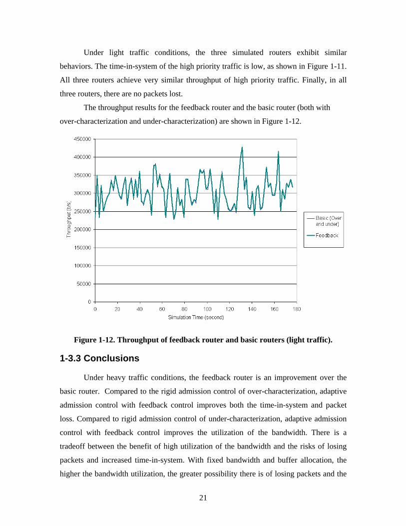
Under light traffic conditions, the three simulated routers exhibit similar
behaviors. The time-in-system of the high priority traffic is low, as shown in Figure 1-11.
All three routers achieve very similar throughput of high priority traffic. Finally, in all
three routers, there are no packets lost.
The throughput results for the feedback router and the basic router (both with
over-characterization and under-characterization) are shown in Figure 1-12.
Figure 1-12. Throughput of feedback router and basic routers (light traffic).
1-3.3 Conclusions
Under heavy traffic conditions, the feedback router is an improvement over the
basic router. Compared to the rigid admission control of over-characterization, adaptive
admission control with feedback control improves both the time-in-system and packet
loss. Compared to rigid admission control of under-characterization, adaptive admission
control with feedback control improves the utilization of the bandwidth. There is a
tradeoff between the benefit of high utilization of the bandwidth and the risks of losing
packets and increased time-in-system. With fixed bandwidth and buffer allocation, the
higher the bandwidth utilization, the greater possibility there is of losing packets and the

22
longer time-in-system will be. The adaptive admission control dynamically balances the
needs of high resource utilization and the goals of timeliness and precision to achieve the
QoS guarantee while maximizing the use of resources.

23
Chapter 2: Router Service Differentiation by Adjusted Weighted Shortest Processing Time Service Discipline
2-1 A-WSPT Service Discipline
Today’s Internet employs a simple service model, named best effort, which employs a
First-Come-First-Serve (FCFS) service discipline to serve the packets at Internet routers.
At the output interface of router, a single queuing is maintained in the buffer and the
packets are served in a first-come-first-serve fashion. The packets are dropped at the tail
of the queue if the buffer is full. The network allocates its resource to its users as best as
it can, making no commitment with regard to service quality, and “all packets are treated
the same without any discrimination or explicit delivery guarantees.” [9] The success of
the Internet is largely contributed to the simplicity of the best effort service model. It is
the end users’ responsibility to maintain the state of connections. The management
overhead in routers is low and cheap. The applications don’t ask for permission before
beginning transmission. No admission control is needed.
Using an FCFS service discipline can, however, lead to performance problems.
When congestion occurs, the queuing delay increases along with the queue length, and
the packets are discarded at the tail of queue when the queuing buffer reaches its
capacity. Most importantly, the resource of the router is allocated on a first-come-first-
service basis, neglecting the service requirement of individual traffic entities and treating
all the packets the same way.
Recent years have witnessed considerable research to extend the Internet
architecture to deliver QoS to support different levels of services. The two most
significant of these efforts are InteServ and DiffServ, which were briefly discussed in
Chapter 1. However, both service models introduce great complexity in implementation
and suggest substantial and radical changes to the existing infrastructures.
The scheduling mechanism employed in a service discipline is a key component
in realizing different levels of services. Therefore, we argue that different levels of
services can be provided by replacing FCFS with a different service discipline without
24
making major changes to internal functions of existing routers. Several service disciplines
have been proposed, such as PGPS, Delay-EDD, Jitter-EDD, and WFQ. A thorough
survey of the literature is available in Gevros, 2001 [9].
In this chapter, we describe a new service discipline called Adjusted Weighted
Shortest Processing Time (A-WSPT), which provides services at different levels while
retaining much of the simplicity of the FCFS service discipline. In A-WSPT, the traffic
stream with a higher weight is treated with lower delay and less packet loss. Packets with
a lower priority are discarded in the event of congestion. The only requirement of
implementing this discipline is that each traffic flow must be assigned a weight to
indicate its relative importance. A-WSPT builds on the ideas found in the Weighted-
Shortest-Processing-Time (WSPT) rule. WSPT was designed to minimize the total
completion time of a finite number of jobs that were ready at beginning time. WSPT
itself is just an extension of the Shortest Processing Time (SPT) rule that associates a
weight factor with each job. The priority of each job is given by the ratio of the weight
factor to the processing time of the packet. The jobs are served in a decreasing order of
the priority [10]. A-WSPT further extends the WSPT to a design that will work in a
networking context. The weight is assigned on a per-flow basis to indicate the priority of
flow. The priority of individual packets is calculated with the weight of the traffic stream.
Another important issue addressed by the A-WSPT service discipline is the large
variance in delay caused by the dynamic service order of WSPT under the condition of
infinite arrivals. In WSPT, arrival packets of higher priority are inserted before those of
lower priority in the service queue. This dynamic insertion may defer the service to low
priority packets for an indefinite period of time. In some case, low priority packets suffer
extreme long delay, or are dropped entirely. As part of A-WSPT, we introduce an
exponential compensation to penalize the long delay of individual packets. The
exponential compensation is based on the intuition of scaling up the priority when the
delay increases.
A queuing system with the A-WSPT service discipline can be conceptualized as a
dynamic priority queuing system with infinite arrivals, in which the packets arrive at the
router without termination in the duration of observation. The priority of each packet is

25
dynamically determined, and the service order is constantly refreshed. The introduction
of the A-WSPT rule is carried out in two steps.
First, the WSPT is customized to the per-flow context. A weight factor is
associated with each traffic stream to claim its service priority. The individual packets
inherit the weight from the associated traffic streams. The priority of each packet is
determined by both the processing time of that packet and the weight of the traffic
stream, as is given by equation
ii
twp = ,
where pi is the priority of packet i, w is the weight associated with the traffic stream it
belongs to, and ti is the service time of that packet. Service time ti is given by the
equation
Φ=
ii
St ,
where Si denotes the size of the packet, and Φ denotes the bandwidth of the link. Thus,
the priority of the packet can be expressed as equation
ii
Swp Φ⋅
= .
The packet is accepted as long as there is enough space available in queuing buffer.
When the remaining queuing buffer is not sufficient for the arrival packet, a preemptive
packet dropper is used to drop packets. The preemptive dropper compares the priority of
arrival packet with that of the packet with lowest priority. If the arrival packet has lower
priority, it is dropped. Otherwise, the packet of lowest priority is dropped from the queue.
The comparison is carried iteratively, until there is enough space to accommodate the
arrival packet.
Packets are stored in the queue in the order of decreasing priority, so that there is
always pk>pl as long as k<l, where k and l denote the position of packets in the queue
respectively. The packet of highest priority is always sent out immediately whenever the
server is available. Those with lower priorities are held in the buffer until they are either
transmitted or otherwise discarded. The order of packets is dynamically refreshed to
reflect the arrival of packets. When an arrival packet is accepted, it is inserted into the

26
queue solely based on the value of its priority. The packet i is inserted between adjacent
packets m and n so that there is always pn<pi<pm, as described in Figure 2-1.
... n m ... 1 Service
i Arrival
Decreasing order of priority
l k
Figure 2-1. Service order and the insertion of the packet.
Second, the packet priority is adjusted to penalize the delay. The insertion of
arrival packets may cause serious delay in queue to some packets with low priority. To
contain long delay caused by dynamic insertion of packets, the priority of a packet is
multiplied by the exponential compensation of delay, which is given by
PTP
ie γλ+
−
, where
Ti stands for the delay in queue of packet, λ and γ are constants scaling the exponential
compensation, and P is the average processing time of incoming packets. The A-WSPT
priority of the packet, then, is given by
PTP
i ieSi
wp γλ+
−Φ=
The compensation increases to 1 when the delay increases from 0 to infinite. The longer
the delay is, the greater the compensation will be. The value of exponential compensation
is solely determined by the delay, given λ, γ and P. The average processing time is given
as a constant empirically. The exponential compensation varies between some initial
level α and maximum 1. The initial level is the compensation value when the delay is
zero, which is given by equation
PP
e γλ
α +−
= 0
with Ti equal to 0.

27
The parameters λ and γ can be determined by setting the upper bound of tolerable delay
in terms of n times the average processing time P and corresponding compensation value
β. That is when Ti rises from 0 to nP, the compensation will increase from α to β. By
solving the equations
PP
e γλ
α +−
= 0 ,
and
PnPP
e γλ
β +−
= ,
we have
nβαβαλ
lnlnlnln−
−= , and
nβα
βγlnln
ln−
=
The priority of packets in the queue is constantly refreshed to reflect the delay each
packet has experienced. After each refresh, the queue is dynamically resorted to maintain
a service order of decreasing priority.
Services are differentiated between traffic streams by assigning different weights.
According to the definition of packet priority, the priority is in direct proportion to the
weight of the associated traffic stream. Increasing the weight of a traffic stream will
increase the priority of all belonging packets. Given identical probability distributions of
packet size for all traffic streams, we argue that the greater weight of a traffic stream
gives higher priority, in a statistical sense, to the belonging packets. As a result, the
packets of a high priority traffic stream have a better chance to be located before those of
a low priority stream in the queue, experiencing shorter delay, and less chance of being
discarded from the tail. Moreover, the controlled variance of delay enables an upper
bound to be set upon the delay.
2-2 Simulations and Experiment
To examine the service guarantee of the A-WSPT service discipline, three separate
routers are modeled using the A-WSPT, the WSPT and the FCFS service disciplines

28
respectively. A comparative experiment is conducted between three router models. The
simulation and experiment are accomplished with the OPNET Modeler of OPNET
Technologies, Inc.
Figure 2-2. Router model in OPNET Modeler.
The router models (Figure 2-2) used in the simulation are composed of two input
ports and an output port, with an IP forwarder module simulating the function of
forwarding the packets from input ports to the output port. Each input port is associated
with three traffic sources. In this study, we assume that all packets come from one of the
two input ports and go to the only output port. A queuing system is used at the output
port. The queuing system is made up of a single queue and uses the service discipline
assigned to that router. A packet sink is connected with the queuing module to collect the
output packets. Since the primary concern of this study is the performance of the service
discipline of the queuing system, we assume that the transmission of packets between the
traffic source, IP forwarder and queuing system incurs neither delay nor packet drop.
Each traffic source generates a traffic stream with a certain service requirement
and a constant average bit rate. Two types of traffic are considered in this simulation –
high priority and low priority. High priority traffic is assigned a larger weight. The
priority of traffic is marked in the Type-of-Service (ToS) field of the IP header of

29
belonging packets. In this study, ToS is set to 7 to indicate high priority traffic, and 0 for
low priority traffic. Since it is a general practice to assume the random arrival process as
a Poisson process, we specify the inter-arrival time of packets as exponentially
distributed. Similarly, the size of packets generated by each source assumes a normal
distribution. The expectation of the rate (bits/second) of the incoming traffic as generated
by each source can be estimated by the ratio of mean packet size and mean inter-arrival
time.
2-3 Results and Discussion
The performance collected from the simulation runs are categorized along the axes
of traffic setting, performance metrics and object of measures. Within each group, the
performances of the three service models are compared. Then, the results are inspected
and the comparison between the models is analyzed. Conclusions are drawn from the
results.
2-3.1 Heavy traffic
Time-in-System
As we observe from Figure 2-3, in the case of overwhelming high priority traffic,
the A-WSPT service discipline demonstrates a marked improvement over both FCFS and
WSPT in the area of time-in-system performance of high priority traffic. In addition,
although we note some variance in the time-in-system under the A-WSPT model, it is a
great improvement over the variance demonstrated by the WSPT.

30
Figure 2-3. Time-in-system of high priority traffic (heavy traffic).
The time-in-system of the FCFS service discipline is shown in Figure 2-4. The
reason that the A-WSPT and WSPT service disciplines are excluded from this figure is
that there was little data to collect because in these disciplines, low priority traffic gets
little chance to be served when traffic conditions are heavy. Compared to the FCFS
service discipline, very few low priority packets are served by the A-WSPT router. The
low priority packets that do get served experience much longer time-in-system, due to the
low priority they have.

31
Figure 2-4. Time-in-system of low priority traffic (FCFS).
Packet loss
Table 2-1 summarizes the packet loss rates of high priority traffic, low priority
traffic and overall traffic under heavy traffic conditions. For high priority traffic, both the
A-WSPT and the WSPT service discipline greatly reduce the packet loss rate. However,
because the overwhelming high priority traffic takes almost all the bandwidth, the packet
loss rate of low priority traffic is extremely high. Thus, for overall traffic, all service
disciplines have roughly the same packet loss rate.
Table 2-1. Packet loss for FCFS, WSPT, and A-WSPT disciplines under heavy traffic.
FCFS WSPT A-WSPT
Premium Service
Traffic
Dropped packets 4555 1043 1150

32
Arrived packets 12583 12583 12583
Packet loss rate 36.2% 8.3% 9.1%
Best Effort Service Traffic
Dropped packets 1945 5483 5353
Arrived packets 5488 5488 5488
Packet loss rate 35.4% 99.9% 97.5%
Overall traffic
Dropped packets 6500 6526 6503
Arrived packets 18071 18071 18071
Packet loss rate 36.0% 36.1% 36.0%
Throughput
The throughput performance for high priority traffic and low priority traffic is
shown in Figure 2-5 and Figure 2-6 respectively. The WSPT service discipline allocates
full bandwidth capacity to high priority traffic, and prohibits the low priority packets
from being served. The A-WSPT discipline allocates a very small portion of bandwidth
to the low priority traffic. The FCFS discipline, instead of discriminating any one stream,
allocates bandwidth roughly in proportion to their incoming rate.

33
Figure 2-5. Throughput of high priority traffic (heavy traffic).
Figure 2-6. Throughput of low priority traffic (heavy traffic).

34
Figure 2-7. Throughput of overall traffic (heavy traffic).
Under overwhelming traffic condition, all three disciplines make use of full bandwidth
capacity, as shown in Figure 2-7.
2-3.2 Light traffic
Time-in-system
The time-in-system of high priority traffic for the A-WSPT, WSPT and FCFS
disciplines is shown in Figure 2-8. A-WSPT and WSPT have a similar time-in-system
performance for premium service traffic under light traffic conditions. Both treat high
priority packets with the shortest delay.
Figure 2-9 shows the time-in-system for lower priority traffic under light traffic
conditions. A-WSPT has a comparable, though slightly higher, time-in-system to the
FCFS service discipline. In this case, compared to WSPT, A-WSPT has a large variance
of time-in-system.

35
Figure 2-8. Time-in-system of high priority traffic (light traffic).
Figure 2-9. Time-in-system of low priority traffic (light traffic).

36
Packet loss
Since the rate of total incoming traffic, including both high priority traffic and low
priority service traffic, is smaller than the bandwidth of the output port, packet loss does
not occur in any of the routers.
Throughput The three service disciplines exhibit similar throughput performance for high
priority (Figure 2-10), low priority (Figure 2-11) and all traffic (Figure 2-12), because,
under light traffic conditions, both high priority and low priority get the share of
bandwidth they need, whatever the service discipline used.
Figure 2-10. Throughput of high priority traffic (light traffic).

37
Figure 2-11. Throughput of low priority traffic (light traffic).
Figure 2-12. Throughput of all traffic (light traffic).

38
2-3.3 Conclusions
We summarize the results as follows. First, the A-WSPT service discipline, just
like WSPT, does differentiate the services between high priority traffic and low priority
traffic by assigning a larger weight to high priority traffic. Under both heavy traffic and
light traffic conditions, A-WSPT achieves better time-in-system performance for high
priority traffic. Second, compared to the WSPT service discipline, A-WSPT substantially
prevents the time-in-system from increasing to extremely high by compensating the time-
in-system. Especially under heavy traffic conditions, A-WSPT effectively contains the
variance of time-in-system of high priority traffic. Finally, however, A-WSPT is not
effective in fair resource allocation between the two traffic streams. High priority traffic
is preemptive, and can deplete the resource exclusively as long as it needs additional
bandwidth.

39
Chapter 3: Providing Quality of Service for a Web Server Using Queuing Disciplines
3-1 QoS Delivery for a Web Server
Providing guarantees on the quality of service is cited as one of the key factors
contributing to the success of an application and a “must” for the next- generation
Internet [11]. While “quality” could mean a number of things for different types of
Internet services (e.g., error-free, reliable data transmission, resolution of images,
foolproof security, etc.), we will focus on QoS as it relates to the timeliness or
responsiveness of the web server in satisfying the clients’ requests during an online
session. In particular, we are interested in evaluating different control policies for the
scheduling or sequencing of jobs in a web server queue based on the expected value of
cycle time of a request; that is, the time between the submission of the request by the
client and the completion of the request. Since the average cycle time metric only
reflects one side of performance, we will also be looking at other performance metrics
that measure responsiveness and efficiency of the web server: tardiness, lateness, average
number of jobs dropped or rejected (for policies that implement admission control), and
average throughput.
3-1.1 Previous Approaches
Several mechanisms have been proposed to address and provide QoS measures
for a web server. Cherkasova et al. [12] developed a session-based admission control
(SBAC) policy to prevent a web server from becoming overloaded, where a session is
defined as a sequence of a client’s individual requests. While their mechanism provides
no differentiation between sessions, the SBAC policy provides a fair guarantee of
completion for any accepted sessions, independent of a session length. However, for e-
commerce sites, longer sessions are generally associated with actual purchases.
Statistical analysis of completed sessions reveals that the overloaded web server
discriminates against longer sessions. Almeida et al. [13] studied the policy of assigning
40
different priorities to the requests according to the requested web content and evaluated
the lateness in handling HTTP requests to the web pages. The strategies that the authors
used are static and limited to affect the scheduling indirectly through the use of process
priority and process blocking.
Li et al. [14] developed a measurement-based admission controlled web server,
which is able to allocate a configurable percentage of the bandwidth to different client
requests. When the server is fully utilized or a particular request has used more than the
allocated bandwidth, the request is discarded. This implies that the admission control
mechanism may drop any session in progress if the session exceeds the allocated
bandwidth. While this policy would benefit several performance measures such as cycle
time, such a strategy may clearly result in unsatisfactory user experience at these sites.
Lu et al. [15] proposed an adaptive architecture based on a feedback control loop to
provide relative delay guarantees for different service classes on a web server under
HTTP 1.1 protocol.
Load balancing is also a popular approach to providing availability by balancing
the service accesses among replicated web servers. Some strategies use the Domain
Name System (DNS) server to govern the resources in a cluster of replicated web servers.
Conti et al. [16] studied the strategy of evenly distributing the processing load among
replicated web servers to provide high levels of QoS. The authors allowed the servers to
be geographically distributed across the Internet. The DNS-based approach is simple, but
has some drawbacks. First, since the DNS service is designed to support data that
changes only infrequently, the approach is not well equipped to propagate changes in a
timely fashion. Secondly, if one of the replicated web servers crashes, the caching of
DNS data makes the services unavailable to all visitors. A solution to this problem is a
“reverse proxy”, which is an HTTP proxy server that operates in the opposite direction of
the commonly known one [17].
While the number of studies addressing the issue of providing QoS for web
servers has recently increased, there is as yet, no simple or comprehensive approach to
designing strategies with a QoS focus, due to the complexities associated with web server
operations. In addition to the academic research on the subject, some organizations have
also tried to address the QoS issue. One of these organizations is the Internet

41
Engineering Task Force (IETF), which implemented and tested a number of protocols or
schemes for this purpose. The Integrated Services (InteServ) initiative was initiated
primarily by the desire to help the Internet support real-time multicast applications. The
InteServ architecture asserts that the underlying Internet architecture can support
multicast backbone (MBONE) type of applications without modification. It proposes that
an extension to the current architecture can be devised to provide capability beyond the
traditional Best-Effort service, in which the client requests are handled on a first-come-
first-served basis, without idling.
QoS in the InteServ model is concerned primarily with the timely delivery of
packets. The InteServ model defines two classes of applications by distinguishing the
application’s dependence on timely delivery of packets [18]. One is called elastic
applications that have no strict requirements for timely delivery of packets. The other
class of applications, which require timely service, is referred to as inelastic or real-time.
The InteServ architecture uses Resource Reservation Setup Protocol (RSVP) [RFC2205]
as its network control protocol to support QoS and traffic control requirements of
application flows by setting up necessary host and router states. RSVP requires signaling
to be deployed end to end in order to provide the requested type of service. However,
this also leads to a scalability problem, which results from the requirement for a signaling
mechanism to establish per-flow traffic states in each router that the path traverses and
prevents deployment of RSVP on the Internet.
The Differentiated Services (DiffServ) architecture simplifies the forwarding path
by moving the complexity of classifying traffic to the edges of the network. DiffServ
supports multiple service levels based on packet marking and per-class management of
routers in the network. DiffServ takes advantage of prioritizing the traffic through
various queue management and scheduling mechanisms.
Compared to InteServ, DiffServ has no explicit signaling protocol that establishes
session paths and maintains state tables with the routers. Packets carry the state
information in the IP headers. Each router handles the packets based on the information
in its differentiated services codeprint (DSCP). This is referred to as per hop behavior
(PHB). Within a DiffServ network, packet scheduling, buffer management, and packet
discard are required to provide differentiated service. Clearly, scheduling schemes that

42
are more sophisticated than the simple FIFO service protocol hold potential to improve
efficiency of a packet-based network.
Several scheduling schemes have been proposed for this purpose. Priority
Queuing (PQ) scheme places packets into the buffer space according to priority, and
processes high-priority packets ahead of the lower priority packets. One problem with
this scheme, however, is that some low priority packets may be discarded or delayed for a
long time.
An enhancement to PQ is Class Based Queuing (CBQ), which permits the users to
assign a particular amount of buffer space to particular traffic classes. This buffer
allocation is static, which is a limitation of the CBQ scheme.
Even the best packet-scheduling algorithm, however, cannot ensure that the buffer
space is fairly allocated among the waiting packets. An ideal buffer management scheme
should make buffer space available to all traffic and at the same time make sure that high
priority traffic will not be deprived of buffer space by lower priority packets. Hence, an
intelligent packet drop scheme is needed. Weighted Fair Queuing (WFQ) with Random
Early Discard (RED) is a scheme that tries to manage the buffer space intelligently by
dropping the packets when there is congestion in the system.
Optimal or effective scheduling of machines and resources in production systems
is a topic that has attracted a lot of attention. For this chapter, we borrow results from the
scheduling literature and research their potential to improve performance of web servers.
We will be studying various scheduling, or more accurately, sequencing rules that have
been shown to yield optimal or effective schedules under certain conditions in production
systems. In particular, we will be implementing and testing the Weighted Shortest
Processing Time first (WSPT), Apparent Tardiness Cost (ATC), and Earliest Due Date
(EDD) scheduling rules to a web server using simulation and observe the performance
improvements these rules may bring.
3-1.2 Web Server Operation
Before presenting our model, an explanation of how web servers operate is useful.
There are three basic elements that make web service possible: Uniform Resource
Locators (URL) for identifying the resources, HyperText Transfer Protocol (HTTP) for

43
transferring the information, and the client-server based architecture. HTTP is stateless,
i.e., each request is processed by the web server independently from previous or
subsequent requests. The client sends a URL request to the web server that provides the
resource. The web server then provides the requested services and returns the results
back to the client. The current version of HTTP, (i.e., HTTP 1.1) uses a mechanism
called persistent connection, which allows multiple requests to reuse the session. The
request is stored in the listen queue of the server’s well-known port, (e.g., 80), when the
web server receives the HTTP 1.1 client’s request. When the incoming requests arrive
faster than the rate at which they are removed from the queue, congestion happens.
Figure 3-1 presents our model for a “QoS web server”. Clients with different
priorities or job types access the web server, consisting of a single unit. The “single
machine” assumption will be relaxed later to allow for multiple requests being processed
simultaneously (i.e., parallel machine case). Once in the queue, each job awaits service
by the server. Upon completion of service, requests exit the system, which defines the
end of the ‘cycle time’. Below, we detail each component defined in our model.
Figure 3-1. Web server QoS model.
Requests Classifier The requests classifier groups the requests so that certain ones are prioritized in
processing. Differentiated service policies aim to provide the highest quality of service to
1
2
n
Clients
Queue Server
Admission Control Scheme
K
...

44
the most important customers. For example, it is common to prioritize the service request
of the clients who pay for the service over the nonpaying clients. Some sites prioritize
requests based on the clients’ access history, IP address, and current status (e.g., a
customer with a full shopping cart or with a purchasing history attains a higher weight
than a customer without a purchasing history or a full cart). Web QoS, developed by
Bhatti and Friedrich [19], allows the incoming requests to be categorized as high,
medium, or low priority based on IP address, requested URL, and so on.
Admission Control Scheme Deferring an incoming request at the very beginning of the transaction, rather than in the
middle is a desirable scheme for an overloaded web server. First, it avoids further
frustration by a client by refusing to accept the requests for which it cannot satisfy the
QoS requirements (e.g., limits on cycle time, lateness and tardiness, etc.). Secondly, it
keeps the queue levels at relatively stable levels, resulting in a less variable output.
We define the QoS factor of an incoming request as
jjjjj PWTDQ −−−= (3-1)
where Dj is the due date of request j, Tj is the arrival time of request j, Wj is the predicted
waiting time (i.e., sum of the processing times of the requests ahead of request j), and Pj
is the expected processing time of request j. According to our assumed admission control
scheme, if Qj is less than zero request j is rejected.
3-1.3 QoS Measures
Timeliness, precision, and accuracy are the attributes of QoS that people generally
use to measure the performance of web servers. We define four QoS measures in this
paper: number of dropped jobs per unit time (i.e., drop rate), average time in system (i.e.,
cycle time), average lateness and throughput. While we consider throughput as one of the
performance metrics, we focus our attention to time in system, drop rate and lateness,
since they represent the QoS characteristics we are most interested in.
Under the best effort and basic DiffServ policies, request drops occur only when
the queue is full. Under the WSTP, ATC, and EDD policies, request drops may happen
at admission control as well as when the queue is full, while requests are waiting in the

45
queue. Time-in-system is used to measure the responsiveness of the web server.
Lateness represents the gap between the completion time and due date, and can be
negative or positive. A negative lateness indicates a request completed before its due
date, and a positive lateness indicates that the request was tardy. Lateness depicts how
well the requirement of the due date of the request is met.
3-2 Discussion of Different Queuing Disciplines
Best Effort Policy
The Internet and most corporate intranets are built with IP protocol, which is a
connectionless protocol that provides no guarantees on service time or relative order of
the packets. For web servers, the incoming requests are placed into a queue and
processed in a First-In-First-Out (FIFO) fashion. In the Best Effort model, there is no
admission control scheme. Hence, if client requests are placed into the queue faster than
they are moved from the queue to be processed, congestion occurs; requests are delayed,
and finally, the requests maybe be discarded. Because of this inherent behavior, the
Internet can only provide a single level of service, that of ‘Best Effort’.
Basic DiffServ Policy
Under the DiffServ policy, requests are categorized into priority classes. The
server always processes the higher priority queue before serving any of the lower priority
queues. DiffServ architectures generally define two kinds of classification: (1) the
behavior aggregate classifier, which selects packets according to the DSCP value on
ingress, and (2) the multifield classifier, which uses a more general set of classification
conditions like IP header field values and source address.
To implement a DiffServ model, we classify the incoming requests into two
categories: high priority and low priority, based on their assigned weights. Figure 3-2
shows two queues: one for high priority requests, another for best effort requests. Both
are serviced in a FIFO manner, but the best-effort queue will only be serviced when there
are no requests waiting in the high priority queue. Again, as in the Best Effort model,
there is no admission control in the basic DiffServ model.
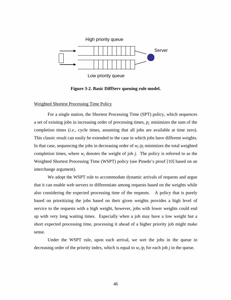
46
Figure 3-2. Basic DiffServ queuing rule model.
Weighted Shortest Processing Time Policy
For a single station, the Shortest Processing Time (SPT) policy, which sequences
a set of existing jobs in increasing order of processing times, pj, minimizes the sum of the
completion times (i.e., cycle times, assuming that all jobs are available at time zero).
This classic result can easily be extended to the case in which jobs have different weights.
In that case, sequencing the jobs in decreasing order of wj /pj minimizes the total weighted
completion times, where wj denotes the weight of job j. The policy is referred to as the
Weighted Shortest Processing Time (WSPT) policy (see Pinedo’s proof [10] based on an
interchange argument).
We adopt the WSPT rule to accommodate dynamic arrivals of requests and argue
that it can enable web servers to differentiate among requests based on the weights while
also considering the expected processing time of the requests. A policy that is purely
based on prioritizing the jobs based on their given weights provides a high level of
service to the requests with a high weight, however, jobs with lower weights could end
up with very long waiting times. Especially when a job may have a low weight but a
short expected processing time, processing it ahead of a higher priority job might make
sense.
Under the WSPT rule, upon each arrival, we sort the jobs in the queue in
decreasing order of the priority index, which is equal to wj /pj for each job j in the queue.
High priority queue
Server
Low priority queue
High priority queue
Server
Low priority queue

47
Weight Only Policy
As a contrast of the WSPT model, we design a Weight Only (WO) model that
uses only ‘weight’ to define the priority of the request to see the influences upon the
model brought by processing time. In this model, the requests that belong to the same
class follow the FIFO queuing discipline to be placed into the queue.
Apparent Tardiness Cost Policy
The Apparent Tardiness Cost (ATC) rule is a composite dispatching rule that
combines the WSPT rule and the Minimum Slack first (MS) rule [10]. The MS policy is a
dynamic dispatching rule that orders jobs in increasing order of slack, where slack of job
j at time t is defined as max {dj- pj - t, 0}. dj denotes the due date of job j and pj denotes
the expected processing time of job j, as before.
Under the ATC rule, jobs are scheduled one at a time; that is, every time the
machine becomes free, a ranking index is computed for each remaining job. The job with
the highest-ranking index is the selected to be processed next. The index is defined as
{ }⎟⎟⎠
⎞⎜⎜⎝
⎛ −−−=
pktpd
pw
tI jj
j
jj
0,maxexp)( , (3-2)
where k is a scaling parameter that can be determined empirically, and p represents the
average of the expected processing times of the remaining jobs in the queue at time t. We
can see that if k is big enough, the ATC rule will reduce to WSPT policy since the ATC
index Ij(t) → wj /pj as k→∝.
Earliest Due Date First Policy
Sequencing a number of jobs in increasing order of their due date, referred to as
the Earliest Due Date first (EDD) policy, minimizes the maximum lateness of a set of
jobs with given due dates and processing times [10]. While we know that EDD is
optimal for the case in which all jobs to be scheduled are available at time zero, it is
harder to find an optimal policy for the case in which jobs are released in different points

48
in time, which reflects our case. The reason is that when preemption of jobs is not
allowed, the optimal schedule is not necessarily a non-idling schedule.
Having noted this point, we adopt the static EDD rule in our web server model by
placing the incoming requests into the queue according to their due date. The requests
with an earlier due date are placed into the front of the queue and processed before the
requests with a later due date.
3-3 Simulation of Different Queuing Rules
We simulate a web server under the policies discussed in section 3-2 using the
OPNET Modeler 8.1.A simulation environment. The simulation experiments were
conducted on a Micron PC with a single Pentium4 1.9GHz CPU and 512MB of RAM
running on Windows 2000 operating system. Figure 3-3 depicts the simulation model
based on the web server system presented in Figure 3-1. Generator 1, generator 2, and
generator 3 modules generate the requests with different weights (i.e., priorities). The
forwarder module forwards the requests to the queue, where the request dropper scheme
is implemented. The requests are then placed into the queue based on different rules.
The sink module destroys the requests after the web server processes them.
Figure 3-3. The topology of the QoS web server simulation.
We define four fields in the data packet format: processing time (denoted as
proc_time), weight, due date and time in system (denoted as TIS). The processing time

49
(i.e., proc_time field in the packet format) represents the time to parse a request and is
assumed to be a function of the packet size, which follows the normal distribution. We
assume that the mean and the standard deviation of packet size are 6000 bytes and 1000
bytes, respectively. Because we focus on the connection and listening queue scheduling
problem of a web server, the processing time is not the time the server spends fetching a
file or executing a CGI program. We calculate the processing time by dividing the
request size by a constant, deterministic service rate. For instance, if the request size is
6000 bytes and the service rate of the server is 240,000 bytes per second, the processing
time for this request is assumed to be 0.025 second.
The weight field is a 4-byte integer that contains the weight information of a
request. The weight value is recorded in the weight field of a request packet when the
request is generated. There are some choices in selecting the proper weight value [19].
For simplicity, we only define three priority classes. In Figure 3-3, generator 1, 2, and 3
generate request arrivals with weights 1, 2 and 4, corresponding to low, medium, high
priority requests.
We expect that under policies that differentiate requests based on priority, the
high priority requests can be processed even when the web server is heavily overloaded
and the medium requests can partly get the service while the low priority requests may
not get the service at all due to request drops. Under the best effort policy, however, all
requests are treated equally. Under the DiffServ policy, requests are classified into low
and high categories; a request with a weight bigger than three is treated as a high priority
request while the remaining requests are categorized and treated as low priority.
The due date field in the packets shows the due date of a request. The due date of
a request is generally a function of the time-criticality of the operation. Some time-
critical applications require the web servers to respond within a specific period. If the
application can’t receive the response as required, the QoS requirements can’t be met. Of
course, whether the application can get the response on time or not depends not only on
how fast the web server processes the request but also on the delay during transmission
on the Internet. How to guarantee a lower bound of delay between routers is out of the
scope of this research. Hence, we focus on the due date that the web server is required to
process a request by and assume that the client will receive the processed request once
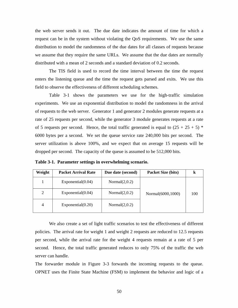
50
the web server sends it out. The due date indicates the amount of time for which a
request can be in the system without violating the QoS requirements. We use the same
distribution to model the randomness of the due dates for all classes of requests because
we assume that they require the same URLs. We assume that the due dates are normally
distributed with a mean of 2 seconds and a standard deviation of 0.2 seconds.
The TIS field is used to record the time interval between the time the request
enters the listening queue and the time the request gets parsed and exits. We use this
field to observe the effectiveness of different scheduling schemes.
Table 3-1 shows the parameters we use for the high-traffic simulation
experiments. We use an exponential distribution to model the randomness in the arrival
of requests to the web server. Generator 1 and generator 2 modules generate requests at a
rate of 25 requests per second, while the generator 3 module generates requests at a rate
of 5 requests per second. Hence, the total traffic generated is equal to (25 + 25 + 5) *
6000 bytes per a second. We set the queue service rate 240,000 bits per second. The
server utilization is above 100%, and we expect that on average 15 requests will be
dropped per second. The capacity of the queue is assumed to be 512,000 bits.
Table 3-1. Parameter settings in overwhelming scenario.
Weight Packet Arrival Rate Due date (second) Packet Size (bits) k
1 Exponential(0.04) Normal(2,0.2)
2 Exponential(0.04) Normal(2,0.2)
4 Exponential(0.20) Normal(2,0.2)
Normal(6000,1000) 100
We also create a set of light traffic scenarios to test the effectiveness of different
policies. The arrival rate for weight 1 and weight 2 requests are reduced to 12.5 requests
per second, while the arrival rate for the weight 4 requests remain at a rate of 5 per
second. Hence, the total traffic generated reduces to only 75% of the traffic the web
server can handle.
The forwarder module in Figure 3-3 forwards the incoming requests to the queue.
OPNET uses the Finite State Machine (FSM) to implement the behavior and logic of a

51
process model. We use a FSM to simulate the processing in the queue. There are 5 states
in the FSM: ‘init’, ‘arrival’, ‘svc_start’, ‘svc_compl’, and ‘idle’.
‘init’ State
The process enters ‘init’ state only once where we initiate the simulation variables and
register the probing statistics. When the simulation begins, the first request will arrive at
the ‘init’ state and then goes to ‘arrival’ state.
‘arrival’ State
When a new request enters into the system and the FSM is in ‘idle’ state, the state
will also transform to ‘arrival’ state.
Best Effort Model. When a request comes, it enters the ‘arrival’ state. If the queue
is already full, the request will be dropped; if not, it will be placed into the queue
by the FIFO rule. This is the way most of the current web servers deal with the
incoming client requests.
Basic DiffServ Model. After a request enters the ‘arrival’ state, we get the
‘weight’ value from the packet. If the weight is bigger than 3 and the high priority
queue is not overflowed, the request will be put into the end of high priority
queue. If the high priority queue is overflowed, the request will be dropped. If the
weight is less than or equal to 3 and the low priority queue is not full, it will be
placed into the end of the low priority queue. If the low priority queue is full, the
request will be discarded.
WSPT Model. First we execute the admission control algorithm: we traverse the
queue to calculate the QoS factor in equation (3-1) for each request in the queue.
If the QoS factor of a request is above 0, it will stay in the queue and wait for
being scheduled to process. If the QoS factor is less than 0, it will be dropped.
After implementation of the Admission Control Scheme, we will get the ‘weight’
value and packet size from a new request that goes into the ‘arrival’ state. We get
the expected processing time of this request by its packet size divided by the
service rate of the queue. Then we get the priority of the incoming request
according to the equation (wj/pj). Now we will try to insert the request into the
queue based on its priority. The requests with bigger priority will be placed ahead
of the requests with less priority. If it is inserted successfully, we will mark

52
‘insert_ok’ as 1. If unsuccessfully, which means that the queue is full, we will
compare the new incoming request’s priority with the priority of the request at the
end of the queue. If the new request’s priority is bigger, we will drop the request
at the end of the queue and insert it according to its priority, and mark ‘insert_ok’
as 1. If the new incoming request has a lower priority, we just discard it.
WO Model. The process is the same as in WSPT model except that we use only
‘weight’ to decide the priority of a request.
ATC Model. As an extension of WSPT, we also implement the Admission
Control Scheme at the very beginning of the ‘arrival’ state. For a new incoming
request, we calculate its index based on equation (3-2) as its priority. We attempt
to insert a request according to its priority into the listening queue and deal with
the insertion action as what WSPT does. We also assign different values to the k,
the scaling parameter, in equation (3-2) to investigate the impacts.
EDD Model. We perform the Admission Control Scheme when the process enters
the ‘arrival’ state. We extract the due date information of a new request from the
packet’s ‘duedate’ field. We use its reciprocal as the priority and try to insert the
request into the queue based on its priority and handle the insertion action as what
WSTP does.
‘svc_start’ State
When the server is not busy and ‘insert_ok’ is marked as 1, the process enters the
‘svc_start’ state from the ‘arrival’ state. Another transformation to the ‘svc_start’ state
happens from the ‘svc_compl’ state when the queue is not empty. In this state, we will
remove a request from the head of the queue and schedule its processing based on its
processing time. When the request is processed, an interrupt occurs and the state is
transformed to ‘svc_compl’. If there are no jobs waiting for processing, then the FSM
transforms to the ‘idle’ state.
A request goes into the sink component in Figure 3-3 after it is dequeued and
processed where the requests are simply destroyed.
We set the simulation duration (i.e., run length) as 4,000 seconds. To capture the
QoS metrics defined above, we use the ‘Bucket’ mode, which is one of the statistics
collection options in OPNet. The Bucket mode collects all of the points over the time

53
interval and calculates the average of all the values collected for that bucket period, to
calculate average performance metrics such as the average TIS and lateness. We use
‘sum/time’, the sum of all the values of points within a particular bucket, divided by the
time duration of the bucket, to capture the drop rate and throughput metrics.
3-4 Experimental Results
In the sections above we introduced our web server QoS models design,
implementation and simulation configuration. In this section, we provide detailed results
on our simulation experiments for the heavy traffic and light traffic cases and provide
intuition on our results for each of the QoS performance measures.
3-4.1 Heavy-traffic Case
We first present the results of the overwhelming traffic scenario.
Time-in-System
TIS
0
0.5
1
1.5
2
2.5
0 1000 2000 3000 4000 5000
Time (Second)
Seco
nd
ATCBEDSEDDWSPTWO
Figure 3-4. Overall time-in-system in the heavy-traffic scenario.
Figure 3-4 shows the TIS performance under the WSPT, ATC, EDD, Best Effort,
WO and Basic DiffServ policies. We take all the requests that get processed into account
and calculate the TIS over time after the 120th second when the system reaches steady
state. We make the following observations:

54
• The overall performance is dramatically enhanced under ATC, EDD, and WSPT
policies. The mean TIS under the Best Effort policy is 2.116 seconds while it is
0.179 seconds under the WSPT policy.
• The Basic DiffServ performs slightly better than Best Effort.
• ATC, EDD, and WSPT, the policies with an admission control scheme, have similar
performance. The admission control scheme discards the requests whose QoS
requirements can’t be met before they are even placed in the queue, which results in
smaller average queue sizes (see Figure 3-5 and Table 3-6) and consequently shorter
TIS. The average queue size of ATC is about 169,802 bytes while under the Best
Effort policy the average queue size is about 499,602 bytes. The processing time also
contributes to the smaller overall TIS of WSPT compared with that under the WO
policy. The overall TIS of WO is about 0.539 seconds.
Queue size
0100000200000300000400000500000600000
0 1000 2000 3000 4000 5000
Time (Second)
Bits
ATCBEDSEDDWSPTWO
Figure 3-5. Queue size in the heavy-traffic scenario.
Table 3-2 shows the mean and standard deviation of TIS for all the three classes
of requests. The TIS of class 1, 2, and 4 under the Best Effort Model is all about 2.11
seconds because there is no differentiation mechanism.
Table 3-2. Time-in-system in heavy-traffic scenario: mean and deviation values.
Type of class Models
1 2 4 Overall

55
Mean 0.523255931 0.08159186 0.039299206 0.184538466 ATC
STD 0.048392924 0.006736874 0.000691119 0.010391973
Mean 2.116473376 2.116473376 2.116167135 2.116167135 Best
Effort STD 0.00478517 0.00478517 0.006119975 0.006119975
Mean 2.265243257 2.264344337 0.039223369 1.982595353 Basic
DiffServ STD 0.026087784 0.026775045 0.000761247 0.006535154
Mean 0.185481416 0.188201039 0.180892617 0.186327018 EDD
STD 0.014389874 0.014481299 0.031294585 0.010743542
Mean 0.499754732 0.081416755 0.039178729 0.178988725 WSPT
STD 0.043456638 0.081416755 0.000668291 0.010373725
Mean 1.966808975 0.082197745 0.039462374 0.539797138 WO
STD 0.050188409 0.007286006 0.000646759 0.030647195
Figure 3-6 shows the TIS of class 4. The high priority class (with weight 4) has
very small TIS under the Basic DiffServ model.
TIS of Class 4
0
0.5
1
1.5
2
2.5
0 1000 2000 3000 4000 5000
Time (second)
Seco
nd
ATCBEDSEDDWSPTWO
Figure 3-6. Time-in-system of Class 4 in the heavy-traffic scenario.
However, the TIS of low priority and medium priority classes under the Basic
DiffServ policy are even longer than that under the Best Effort policy, as shown in
Figures 3-7 and 3-8. For the ATC and WSPT models, the TIS of class 4 is quite small,
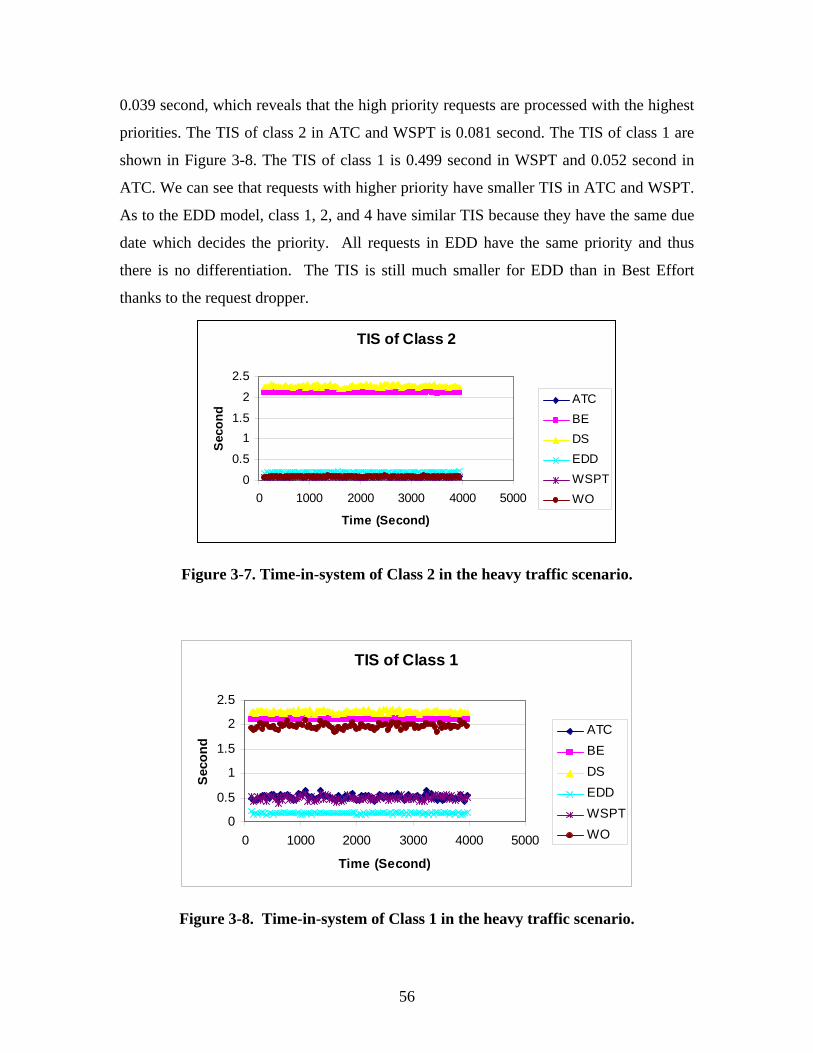
56
0.039 second, which reveals that the high priority requests are processed with the highest
priorities. The TIS of class 2 in ATC and WSPT is 0.081 second. The TIS of class 1 are
shown in Figure 3-8. The TIS of class 1 is 0.499 second in WSPT and 0.052 second in
ATC. We can see that requests with higher priority have smaller TIS in ATC and WSPT.
As to the EDD model, class 1, 2, and 4 have similar TIS because they have the same due
date which decides the priority. All requests in EDD have the same priority and thus
there is no differentiation. The TIS is still much smaller for EDD than in Best Effort
thanks to the request dropper.
TIS of Class 2
0
0.5
11.5
2
2.5
0 1000 2000 3000 4000 5000
Time (Second)
Seco
nd
ATCBEDSEDDWSPTWO
Figure 3-7. Time-in-system of Class 2 in the heavy traffic scenario.
TIS of Class 1
0
0.5
1
1.5
2
2.5
0 1000 2000 3000 4000 5000
Time (Second)
Seco
nd
ATCBEDSEDDWSPTWO
Figure 3-8. Time-in-system of Class 1 in the heavy traffic scenario.

57
Drop Rate
Drop
0
5
10
15
20
25
0 1000 2000 3000 4000 5000
Time (Second)
Seco
nd
ATCBEDSEDDWSPTWO
Figure 3-9. Overall drop in the heavy traffic scenario.
Drop of Class 4
0
0.5
1
1.5
2
2.5
0 1000 2000 3000 4000 5000
Time (second)
Pack
ets
ATCBEDSEDDWSPTWO
Figure 3-10. Drop of Class 4 in overwhelming scenario.
Figure 3-9 shows the overall drop rate. Figure 3-10 depicts the drop of the high
priority requests. The average drop rate for high priority requests under the Best Effort
policy is about 1.4 packets per second and 1.38 packets per second under EDD (see Table
3-3). EDD provides only a slight improvement in drop rate because the request with the
earliest due date is given priority in processing under EDD. In this simulation, we set the

58
same due date for all three classes of requests which leads to no differentiation between
the three classes.
Almost no high priority requests are dropped under the Basic DiffServ policy.
However, more requests in low and medium priority classes are dropped even compared
to Best Effort. This reveals that Basic DiffServ discriminates the Best Effort requests to
give premium requests better performance. This verifies the design that only when there
is no high priority request waiting for processing can a low priority request get the chance
to be processed.
ATC and WSPT offer good granularity and differentiation. There is also almost
no high priority requests dropped under the ATC and WSPT policies (0.005
packets/second in WSPT, and 0.007 packets/second in ATC). The low priority requests,
however, have a drop rate of about 15 packets per second under the WSPT and ATC
policies, as shown in Figure 3-12. So, the requests with higher priority are processed at
the expense of low priority requests.
Drop of Class 2
-2
0
2
4
6
8
10
0 1000 2000 3000 4000 5000
Time (second)
Pac
kets
ATCBEDSEDDWSPTWO
Figure 3-11. Drop of Class 2 in overwhelming scenario.

59
Drop of Class 1
0
5
10
15
20
25
0 1000 2000 3000 4000 5000
Time (second)
Pac
kets
ATCBEDSEDDWSPTWO
Figure 3-12. Drop of Class 1 in overwhelming scenario.
In Table 3-3, we note that the overall drop rate is at the same level for all the
models. This is because the service rate of the queue is fixed at 240,000 bits per second
and the simulation setting is identical for all the models.
Table 3-3. Drop in heavy-traffic scenario.
Type of class Models
1 2 4 Overall
Mean 15.62565822 0.007989691 0 15.63442111ATC
STD 1.414766351 0.012126125 0 1.419334222
Mean 6.793182074 6.897147962 1.407688479 15.09766343Best Effort
STD 0.688833983 0.655430033 0.201257757 1.310141545
Mean 7.5006563 7.59302425 0 15.09353971Basic DiffServ
STD 0.775397906 0.662476673 0 1.308048687
Mean 6.92495467 7.01436005 1.38964126 15.62392374EDD
STD 0.724070713 0.659029458 0.212349655 1.375694534
WSPT Mean 15.5545242 0.005346005 0 15.5601943

60
STD 1.371508209 0.008310796 0 1.375888456
Mean 15.75464245 0.000773196 0 15.75541565WO
STD 1.427166528 0.000564566 0 1.428159499
Lateness
Table 3-4 shows the results of Lateness. As we define Lateness as TIS deducted
by the due date, we find that ATC, EDD, and WSPT models have negative Lateness,
which means they meet the lateness QoS requirement. In DiffServ only requests of class
4 can get the service before the due date. The Best Effort Model can’t meet the lateness
requirements at all.
Table 3-4. Lateness in heavy-traffic scenario.
Type of class Models
1 2 4 Overall
Mean -1.528289244 -1.921393994 -1.960512063 -1.829788613ATC
STD 0.043709876 0.015548354 0.03111366 0.013234516
Mean 0.115708211 0.114391906 0.11358857 0.114937899Best Effort
STD 0.017526331 0.018718165 0.04003511 0.01217135
Mean 0.26508576 0.26213268 -1.960587 -0.01839025Basic DiffServ
STD 0.03196414 0.03435459 0.0310609 0.0130461
Mean -1.612081557 -1.612478523 -1.61480927 -1.612503186EDD
STD 0.019171375 0.019259405 0.03277927 0.016589612
Mean -1.527947347 -1.921466671 -1.960623133 -1.829577936WSPT
STD 0.042454893 0.015487681 0.031133791 0.014023748
Mean -0.392350188 -1.920620298 -1.960345972 -1.549753094WO
STD 0.024025049 0.015704897 0.030984531 0.028747725

61
Throughput
Table 3-5 contains the results on average throughput. The results are consistent
with those contained in Table 3-3. As can be expected, higher drop rate results in smaller
throughput. We find that with the same overall throughput, ATC and WSPT successfully
differentiate the throughput among the three classes of requests. The Basic DiffServ
policy yields a higher throughput of high priority requests compared to that under the
Best Effort policy, which provides no differentiation between the requests.
Table 3-5. Throughput in heavy-traffic scenario.
Type of class Models
1 2 4 Overall
Mean 59144.62807 150588.3688 30429.08981 240161.1892ATC
STD 5311.398924 4981.326976 2263.328942 13.70711604
Mean 109007.5019 109181.9109 21973.07728 240161.146Best Effort
STD 2699.866684 2778.473433 1825.844209 13.63159207
Mean 104738.9537 104993.1148 30429.02813 240159.9215Basic DiffServ
STD 2770.724671 2877.987539 2262.411586 1.519452587
Mean 108908.678 109155.7446 22096.96516 240160.2943EDD
STD 3041.214913 3238.332632 1860.560017 5.257452625
Mean 59128.50729 150604.6331 30429.04182 240161.271WSPT
STD 5331.385047 4986.82248 2258.003664 12.83305048
Mean 59101.43066 150630.4305 30429.03291 240160.039WO
STD 5346.217383 5001.39114 2260.481318 2.591546896
Average Queue Size
The average queue size under each of the policies is shown in Table 3-6. The
average queue size under ATC and WSPT are only about one third of that under the Best
Effort and DiffServ policies. The smaller queue size contributes to the smaller average
TIS under these two policies. We also find that the average queue size of the Basic

62
DiffServ is about 31,669 bytes smaller than that of the Best Effort because of its priority
queuing policy.
Table 3-6. Average queue size for heavy-traffic scenario.
3-4.2 Light-Traffic Case
Time-In-System
Table 3-7. Parameter settings in light-traffic scenario.
Weight Packet Arrival Rate Due date (second) Packet Size (bits) k
1 Exponential(0.08) Normal(2,0.2)
2 Exponential(0.08) Normal(2,0.2)
4 Exponential(0.2) Normal(2,0.2)
Normal(6000,1000) 100
Table 3-7 shows the parameters we use for the light traffic case. Figure 3-13
shows the overall TIS of the ATC, Best Effort, Basic DiffServ, EDD, WSPT and WO
policies. The performances are quite similar, at about 0.062 second. This is because the
incoming traffic is 75% of the service rate of the web server and there is almost no
congestion in the queue as shown in Figure 3-14. The queue size of these models is in
the same level. For example, WSPT has an average queue size of about 6,764.449711
bytes as shown in Figure 3-14 and Table 3-12.
Models ATC Best Effort DiffServ EDD WSPT WO
Mean 169802.9935 499602.1988 215178.9891 170659.3655 248627.5597 467932.8914Average
Queue
Size
(bits) STD 10201.86113 1011.774575 11632.35623 10196.18705 8097.747311 1183.825111

63
TIS
0
0.02
0.04
0.06
0.08
0.1
0 1000 2000 3000 4000 5000
Time (Second)
Sec
ond
ATCBEDSEDDWSPTWO
Figure 3-13. Overall time-in-system in light-traffic scenario.
Queue size
0
2000
4000
6000
8000
10000
12000
14000
0 1000 2000 3000 4000 5000
Time (Second)
Bits
ATCBEDSEDDWSPTWO
Figure 3-14. Queue size in light-traffic scenario.
Table 3-8. Time-in-system in light-traffic scenario.
Type of class Models
1 2 4 Overall
Mean 0.08767569 0.046046819 0.038381015 0.062116768ATC
STD 0.012771224 0.002349674 0.001027451 0.005996689
Mean 0.062669004 0.062571566 0.062510799 0.06259972Best
Effort STD 0.007166764 0.007126773 0.00711038 0.006908039

64
Mean 0.068026702 0.068017621 0.035670696 0.062600114Basic
DiffServ STD 0.008446438 0.008466646 0.000838722 0.006905134
Mean 0.062898659 0.062437867 0.062127023 0.062565073EDD
STD 0.008240095 0.007204041 0.008842558 0.006772264
Mean 0.091027432 0.044015203 0.035672294 0.06221866WSPT
STD 0.013470482 0.002179968 0.000842854 0.006230094
Mean 0.091847391 0.04404861 0.035675891 0.062576618WO
STD 0.014979064 0.002205344 0.000836807 0.006812168
We also note that TIS of the high priority requests under the ATC, WSPT, Basic
DiffServ, and WO policies is smaller than that under the Best Effort and EDD policies
(see Figure 3-15 and Table 3-8). TIS of the medium priority requests under the ATC,
WSPT and WO policies is smaller than that under the Best Effort and EDD policies (see
Figure 3-16). Hence, requests with higher priorities have precedence over requests with
lower priorities. However, TIS of the low priority requests under the ATC, WSPT, and
WO policies are longer than that under the Best Effort and EDD policies (see Figure 3-
17).
TIS of Class 4
0
0.02
0.04
0.06
0.08
0.1
0 1000 2000 3000 4000 5000
Time (Second)
Seco
nd
ATCBEDSEDDWSPTWO
Figure 3-15. Time-in-system of Class 4 in light-traffic scenario.

65
TIS of Class 2
0
0.02
0.04
0.06
0.08
0.1
0.12
0 1000 2000 3000 4000 5000
Time (Second)
Sec
ond
ATCBEDSEDDWSPTWO
Figure 3-16. Time-in-system of Class 2 in light-traffic scenario.
TIS of Class 1
00.020.040.060.080.1
0.120.140.160.18
0 1000 2000 3000 4000 5000
Time (Second)
Sec
ond
ATCBEDSEDDWSPTWO
Figure 3-17. Time-in-system of Class 1 in light-traffic scenario.
Drop Rate
Figure 3-18 includes the overall drop rate information. There is no drop at all
under the Best Effort and Basic DiffServ policies (see Table 3-9). There are very small
amounts of requests dropped in ATC, WSPT, EDD and WO due to the admission control

66
scheme. As we can see, the average drop rate in the WSPT model is about 0.003865979
requests per second. We also find that all the drops occur only in the class of low priority
requests (see Figure 3-19 and Table 3-9).
Drop
-0.05
0
0.05
0.1
0.15
0.2
0.25
0 1000 2000 3000 4000 5000
Time (Second)
Pac
kets
ATCBEDSEDDWSPTWO
Figure 3-18. Overall drop in light-traffic scenario.
Drop
-0.05
0
0.05
0.1
0.15
0.2
0.25
0 1000 2000 3000 4000 5000
Time (Second)
Pack
ets
ATCBEDSEDDWSPTWO
Figure 3-19. Drop of Class 1 in light-traffic scenario.
Table 3-9. Drop in light-traffic scenario.
Type of class Models
1 2 4 Overall
ATC Mean 0.006701031 0 0 0.006701031
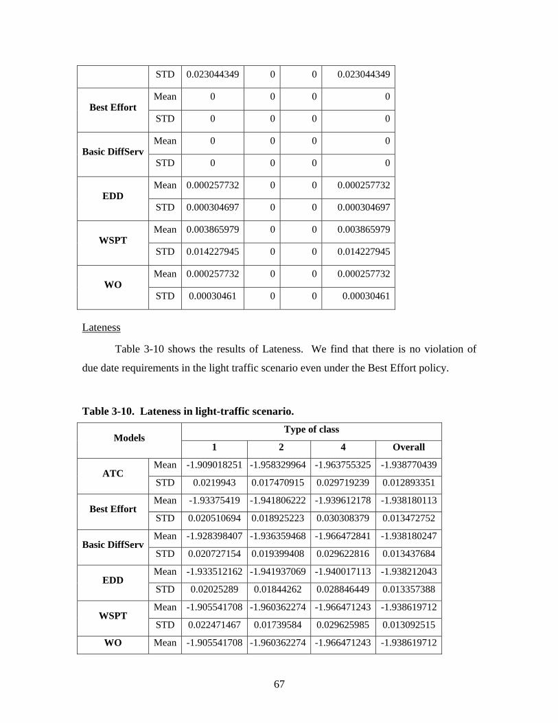
67
STD 0.023044349 0 0 0.023044349
Mean 0 0 0 0Best Effort
STD 0 0 0 0
Mean 0 0 0 0Basic DiffServ
STD 0 0 0 0
Mean 0.000257732 0 0 0.000257732EDD
STD 0.000304697 0 0 0.000304697
Mean 0.003865979 0 0 0.003865979WSPT
STD 0.014227945 0 0 0.014227945
Mean 0.000257732 0 0 0.000257732WO
STD 0.00030461 0 0 0.00030461
Lateness
Table 3-10 shows the results of Lateness. We find that there is no violation of
due date requirements in the light traffic scenario even under the Best Effort policy.
Table 3-10. Lateness in light-traffic scenario. Type of class
Models 1 2 4 Overall
Mean -1.909018251 -1.958329964 -1.963755325 -1.938770439 ATC
STD 0.0219943 0.017470915 0.029719239 0.012893351
Mean -1.93375419 -1.941806222 -1.939612178 -1.938180113 Best Effort
STD 0.020510694 0.018925223 0.030308379 0.013472752
Mean -1.928398407 -1.936359468 -1.966472841 -1.938180247 Basic DiffServ
STD 0.020727154 0.019399408 0.029622816 0.013437684
Mean -1.933512162 -1.941937069 -1.940017113 -1.938212043 EDD
STD 0.02025289 0.01844262 0.028846449 0.013357388
Mean -1.905541708 -1.960362274 -1.966471243 -1.938619712 WSPT
STD 0.022471467 0.01739584 0.029625985 0.013092515
WO Mean -1.905541708 -1.960362274 -1.966471243 -1.938619712

68
STD 0.022471467 0.01739584 0.029625985 0.013092515
Throughput
Table 3-11 contains the results on the throughput metric. Since the incoming
traffic and service rates are the same under all of the policies, they produce almost the
same level of throughput in the light traffic scenario, since the system is stable and able
to handle the incoming traffic. The throughput of the Best Effort and Basic DiffServ
policies are a little higher than that under the other policies since no requests are dropped,
resulting in a higher arrival (and hence, throughput) rate.
Table 3-11. Throughput in light-traffic scenario.
Type of class Models
1 2 4 Overall
Mean 75112.80021 74756.6419 30122.96162 179991.1079ATC
STD 3585.030425 3301.072765 2293.579455 5213.360062
Mean 75153.08191 74756.6419 30122.96162 180031.3896Best Effort
STD 3599.10931 3311.927752 2284.944747 5228.480786
Mean 75153.08191 74756.6419 30122.96162 180031.3896Basic
DiffServ STD 3596.599427 3309.438904 2293.930355 5228.508383
Mean 75151.53655 74756.6419 30122.96162 180029.8442EDD
STD 3590.526122 3306.806282 2280.50883 5228.891594
Mean 75129.66799 74756.6419 30122.96162 180007.9757WSPT
STD 3595.088318 3299.409243 2293.996179 5227.263631
Mean 75151.53681 74756.6419 30122.96162 180007.9757WO
STD 3593.143244 3299.204783 2293.94109 5227.263631
Queue size
Tables 3-12 show the average queue size under each one of the policies. Since there is
almost no congestion in the system under this light traffic, the average queue length
under the different policies is quite similar at around 6,000 bits. The smaller queue size
contributes to the smaller overall TIS compared to those observed in the heavy traffic
case.

69
Table 3-12. Average queue size in light-traffic scenario.
3-5 Conclusions
In this chapter, we demonstrated how to model a web server as a single machine
and applied the WSPT, ATC, and EDD queuing disciplines to differentiate the services
and thus to provide QoS to nowadays Best Effort web servers.
We proposed that most current web servers could be modeled via the Best Effort
Model. From the simulation results we verified that the Best Effort Model couldn’t
provide differentiated service at all.
In the Basic DiffServ Model, incoming requests are classified to two levels: low
priority and high priority. High priority requests always have precedence over low
priority requests. Low priority requests are processed only when there are no requests in
the high priority queue. From the simulation results we find that the performance of high
priority requests is guaranteed: no drop and low TIS. Basic DiffServ is easy to understand
and implement. However, as we can see from the results, Basic DiffServ must be used
with care. A large volume of high priority requests will easily starve the best effort
requests; the best effort requests will never be processed if high priority requests are
always in the high priority queue. In our simulation, the ratio of best effort requests and
high priority requests is 10:1. Therefore, the Basic DiffServ Model should only be used
for mission-critical traffic to ensure the amount of the high priority requests is limited to
a small portion of the overall traffic.
We introduced a Request Drop Scheme, which contributes to the tremendous
improvement in the TIS. Thanks to the Admission Control Scheme, the overall TIS of the
WSPT, ATC, and EDD Models is less than 10% of the overall TIS of the Best Effort and
Models ATC Best Effort DiffServ EDD WSPT WO
Mean 6733.640516 6768.938395 6766.479461 6742.812166 6764.449711 6768.725789Average
Queue
Size
(bits) STD 1345.415357 1420.724057 1413.723684 1366.507132 1410.745253 1421.345737

70
Basic DiffServ Models. This reveals that the Admission Control Scheme is effective to
maintain timeliness for an overwhelmed web server.
We have shown that the WSPT and ATC dispatching rules can be used to provide
differentiated services. Instead of simply using the weight, WSPT combines it with
processing time to determine the priority of a request. Unlike Basic DiffServ, in which
the high priority requests always have precedence over the Best Effort requests, a request
with low weight but short processing time in WSPT and ATC still has the chance to be
processed before a request with high weight and longer processing time. ATC is a
composite of WSPT and MS. We perceived that in our case the main factor in ATC is
WSPT, not MS. From the simulation results, the performance of ATC is quite similar to
WSPT when the scaling parameter k is set to 100. We also create a scenario of ATC with
different scaling parameters of 1, 50, 100, 1000 and 10000. Figure 3-20 shows that when
k is as small as 1 the overall TIS is longer than k equals 50. The TIS is quite similar when
k is equal to or bigger than 50. We also note that there is no differentiation between
requests when k is 1 and that ATC is converging to WSPT when k is 10,000 as expected.
TIS
0
0.05
0.1
0.15
0.2
0.25
0.3
0.35
0 1000 2000 3000 4000 5000
Time (Second)
Sec
ond
k=1k=50k=100k=1000k=10000
Figure 3-20. Overall time-in-system of ATC with different scaling parameters.
We can also safely conclude that our QoS models not only provide good
performance when the server is overloaded but also work well under the light traffic
condition. In the light-traffic scenario, the QoS models provide better TIS for high
71
priority requests at the cost of a very small amount of drop of lower priority requests and
slightly longer TIS for lower priority requests, and thus, the cost/benefits get balanced.
However, as Pinedo stated [10], real-world scheduling problems are different
from the mathematical models in academia. For example, WSPT is a static rule, which is
not time dependent. It assumes that there are n jobs to be scheduled and the problem is
done after the n jobs are scheduled. For a web server, the requests are submitted by
clients continuously. WSPT may not be the optimal scheduling rule to gain the minimum
total weighted completion time. Another important aspect of the differences is that the
stochastic models usually use special distributions which may not represent the behaviors
of the real system closely. Here we use request size divided by service rate to decide the
processing time of a request. Request size follows the normal distribution. For a web
server, the processing time of a request may be influenced by the load and configuration
of the web server.
In spite of so many differences, the scheduling rules in manufacturing provide
valuable insights into the scheduling problems in information infrastructures. From the
results of our research, some manufacturing scheduling rules may be used to develop the
framework for QoS enabled web servers.
72
REFERENCES 1. S. Garfinkel, and G. Spafford (1996). Practical UNIX & Internet Security.
Cambridge: O’Reilly & Associates.
2. G. Huston, Internet Performance Survival Guide. New York, Wiley, 2000, pp. 9.
3. R. Braden, D. Clark, and S. Shenker, “Integrated services in the Internet architecture:
an overview,” Request for Comments (Informational) 1633, Internet Engineering
Task Force, June 1994. Available: http://www.ietf.org/rfc.html.
4. S. Blake, D. Black, M. Carlson, E. Davies, Z. Wang, and W. Weiss “An architecture
for differentiated service,” Request for Comments (Informational) 2475, Internet
Engineering Task Force, Dec. 1998. Available: http://www.ietf.org/rfc.html.
5. Jim Kurose, “Open issues and challenges in providing quality of service guarantees in
high-speed networks”, ACM SIGCOMM Computer Communication Review, vol. 23
n.1, pp.6-15, Jan. 1993.
6. B. Sabata, S. Chatterjee, M. Davis, J. J. Sydir, T. F. Lawrence, “Taxomomy of QoS
Specifications,” in 3rd Workshop on Object-Oriented Real-Time Dependable
Systems, 1997, pp. 100-107.
7. A. K. Parekh and R. G. Gallager, “A Generalized Processor Sharing Approach to
Flow Control in Integrated Services Networks: The Single-Node Case,” IEEE/ACM
Transactions on Networking, vol. 1, no. 3, pp. 344-357, June 1993.
8. Howard L. Harrison, John G. Bollinger, Introduction to Automatic Controls, 2nd
Edition. New York: Harper & Row, 1969, pp. 159-182.
9. Panos Gevros, et al, “Congestion Control Mechanisms and the Best Effort Service
Model”, IEEE Network, 2001
10. Michael Pinedo, Chapter 3, “Scheduling: Theory, Algorithms, and Systems”, Prentice
Hall, 1995.

73
11. Strnadl, C., 2002, At your Service: QoS for the Internet, IEEE Multimedia, 93-95.
12. Cherkasova, L. and Phaal, P., 2002, Session-Based Admission Control: A mechanism
for Peak Load Management of Commercial Web Sites, IEEE TRANSACTIONS ON
COMPUTERS, 13 (6), 669-685.
13. Almeida, J., Dabu, M., Manikutty, A. and Cao P., 1998, Providing Differentiated
Levels of Services in Web Content Hosting, First Workshop on Internet Server
Performance, Madison, WI.
14. Li, K. and Jamin, S., 2000, A measurement-Based Admission-Controlled Web
Server, Proc IEEE INFCOM 2000.
15. Lu, C., Abdelzaher, T. F., Stankovic, J. A. and Son, S. H., 2001, A FeedBack Control
Approach for Guaranteeing Relative Delays in Web Servers, IEEE Real-Time
Technology and Application Symposium (RTAS’ 2001), Taipei, Taiwan.
16. Conti, M., Gregori, E. and Panzieri, F., 1999, Load Distribution among Replicated
Web Servers: A Qos-Based Approach, Second Workshop on Internet Server
Performance in conjunction with ACM SIGMETRICS 99/FCRC, Atlanta, GA.
17. Engelschall, R. S., 1998, Load Balancing Your Web Site, Practical Approaches for
Distributing HTTP traffic, http://www.webtechniques.com/archives/1998/engelschall
18. Lzzo, P., 2000, Gigbit networks: standards and schemes for next-generation
networking, (John Wiley & Sons, Inc.), chapter 6, pp. 177-233.
19. Bhatti, N. and Friedrich, R., 2000, Web Server Support for Tiered Services, IEEE
Network, 13 (5).
Recommended