Quantifying reworking and accumulation rates in a plaggic anthrosol using feldspar single-grain luminescence dating
MSC THESIS
ANNIKA VAN OORSCHOT
Supervisors: Tony Reimann and Jakob Wallinga
Chair group: Soil Geography and Landscape (SGL)
Student number: 940202623100
Submitted: March 2018
2
Abstract Plaggic anthrosols are the soils resulting from fertilisation of arable land with a mixture of manure and
plaggen sods cut from the rich organic Ah horizon of surrounding soils. During the Middle Ages, this
self-sustaining type of agriculture was very productive. In the European sand belt, which covers parts
of north-western Europe, Poland and the Baltic region, plaggic agriculture led to gradual accumulation
of soil material and elevation of the soil surface. The rates of accumulation and of biological and
anthropogenic soil reworking have not yet been clarified for plaggic soils while they might hold
valuable information on historical agricultural practices in these soils. Such information will not only
increase our understanding of historical agriculture, it might also help us improve future management
of agricultural soils. The dual goal of this research is to provide insight in the history of a plaggic
anthrosol and to test a newly developed feldspar single-grain luminescence dating protocol by
Reimann et al. (2012). In this study the accumulation and reworking rates are calculated based on the
ages of single grains of feldspar. A profile of a plaggic anthrosol near Denekamp in the east of the
Netherlands was sampled. This location was selected because of the unique availability of recently
determined, independent quartz OSL ages (Smeenge in preparation). The results indicate that plaggic
agriculture at this location started around the beginning of the High Middle Ages (1000-1300 AD),
which coincide with the Medieval Warm Period (950-1250 AD). This might suggest that the population
growth and improved agricultural techniques in the High Middle Ages together with the improved
climatic conditions of the Medieval Warm Period led to the cultivation of the sampled location for
plaggic agriculture. High accumulation rates were found for a period extending far beyond the Middle
Ages into the late 19th century. This leads to the conclusion that plaggic agriculture existed from the
High Middle Ages until the late 19th century. Soil reworking was quantified by effective soil reworking
rates rather than by the more commonly used apparent soil reworking rates. The effective soil
reworking rate also accounts for the fraction of grains that do not participate in soil reworking. The
effective soil reworking rates in the plaggic layers of the investigated plaggic anthrosol are one to two
orders of magnitude larger than the reworking rates in the cover sand parent material, pointing out
the difference between natural and anthropogenic soil mixing. The feldspar single-grain ages are all
consistent with independent age estimates at the same location. An important advantage of dating
single feldspar grains over dating single quartz grains is that a much larger percentage of the feldspar
grains emits a suitable luminescence signal. This property combined with the consistency of the ages
with independent age estimates from a well-established method and with the dates of historical events
shows the potential of this new method for future applications.
3
Contents Abstract ................................................................................................................................................... 2
Introduction ............................................................................................................................................. 5
Plaggic anthrosols ....................................................................................................................................... 5
Luminescence dating of plaggic anthrosols ................................................................................................ 7
Research objectives ................................................................................................................................. 9
Background ............................................................................................................................................ 10
Luminescence dating................................................................................................................................. 10
Palaeodose ............................................................................................................................................ 11
Dose rate ............................................................................................................................................... 12
Measuring soil mixing using single-grain luminescence ........................................................................... 13
Single-grain quartz dating ..................................................................................................................... 14
Single-grain feldspar dating ................................................................................................................... 15
Analysis of single-grain distributions ........................................................................................................ 16
Weighted mean age models.................................................................................................................. 17
Minimum age model and maximum age model ................................................................................... 17
Finite mixture model ............................................................................................................................. 17
Sampling location and site description ................................................................................................. 19
Experimental methods and details........................................................................................................ 20
Soil description and classification ............................................................................................................. 20
Sampling .................................................................................................................................................... 21
Measurements .......................................................................................................................................... 21
Dose rate ............................................................................................................................................... 21
Equivalent dose ..................................................................................................................................... 22
Minimum age calculation ...................................................................................................................... 24
Minimum age model ................................................................................................................................. 25
Iterated weighted mean age ..................................................................................................................... 26
Selection of signal and age model............................................................................................................. 26
Soil reworking rates ............................................................................................................................... 29
Plaggen accumulation rates .................................................................................................................. 31
Discussion and interpretation ............................................................................................................... 33
Feldspar single-grain dating of plaggic soils in context ............................................................................. 33
Start of plaggic agriculture ........................................................................................................................ 33
Natural and anthropogenic soil reworking ............................................................................................... 34
4
Historical accumulation of plaggen ........................................................................................................... 35
Conclusions ............................................................................................................................................ 38
Acknowledgements ............................................................................................................................... 39
References ............................................................................................................................................. 40
Appendix ................................................................................................................................................ 45
pIRIR sample descriptions ......................................................................................................................... 45
Radial plots ............................................................................................................................................ 45
Equivalent dose distributions ................................................................................................................ 47
IRSL sample descriptions ........................................................................................................................... 50
Radial plots ............................................................................................................................................ 50
Equivalent dose distributions ................................................................................................................ 52
Result tables .............................................................................................................................................. 55
Overdispersion ...................................................................................................................................... 55
Ages ....................................................................................................................................................... 55
Soil reworking rates ............................................................................................................................... 55
Plaggen accumulation rates .................................................................................................................. 56
5
Introduction
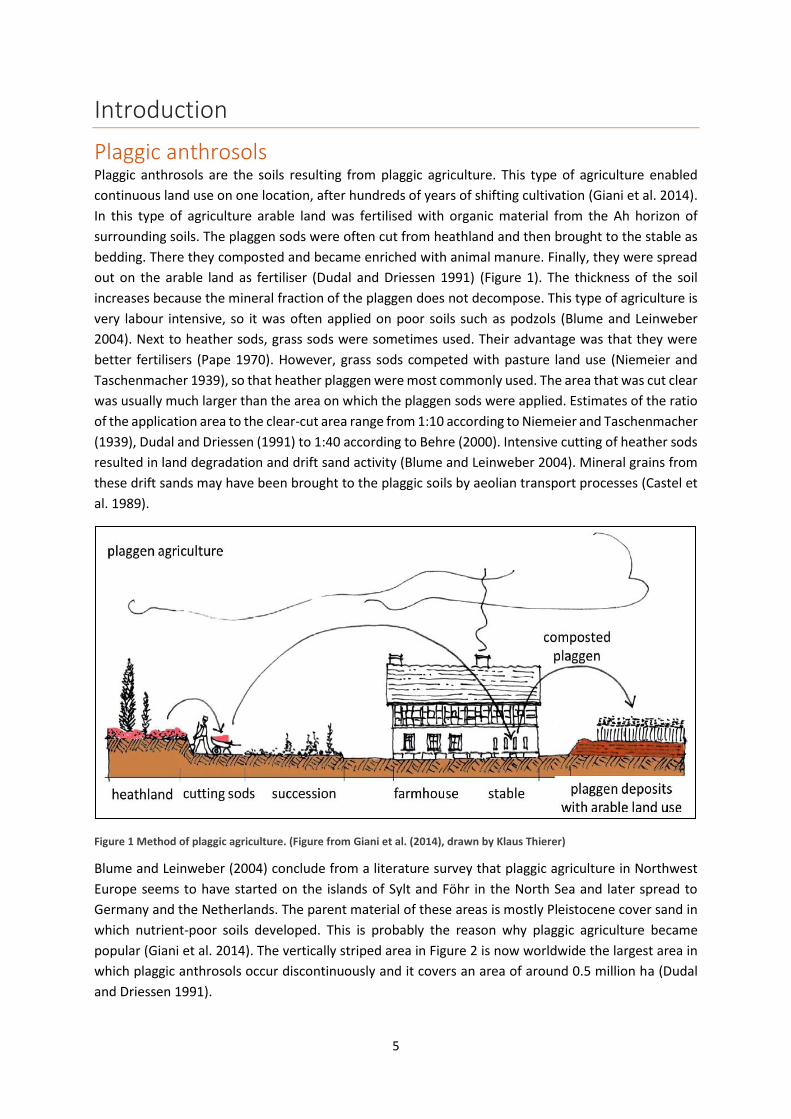
Plaggic anthrosols Plaggic anthrosols are the soils resulting from plaggic agriculture. This type of agriculture enabled
continuous land use on one location, after hundreds of years of shifting cultivation (Giani et al. 2014).
In this type of agriculture arable land was fertilised with organic material from the Ah horizon of
surrounding soils. The plaggen sods were often cut from heathland and then brought to the stable as
bedding. There they composted and became enriched with animal manure. Finally, they were spread
out on the arable land as fertiliser (Dudal and Driessen 1991) (Figure 1). The thickness of the soil
increases because the mineral fraction of the plaggen does not decompose. This type of agriculture is
very labour intensive, so it was often applied on poor soils such as podzols (Blume and Leinweber
2004). Next to heather sods, grass sods were sometimes used. Their advantage was that they were
better fertilisers (Pape 1970). However, grass sods competed with pasture land use (Niemeier and
Taschenmacher 1939), so that heather plaggen were most commonly used. The area that was cut clear
was usually much larger than the area on which the plaggen sods were applied. Estimates of the ratio
of the application area to the clear-cut area range from 1:10 according to Niemeier and Taschenmacher
(1939), Dudal and Driessen (1991) to 1:40 according to Behre (2000). Intensive cutting of heather sods
resulted in land degradation and drift sand activity (Blume and Leinweber 2004). Mineral grains from
these drift sands may have been brought to the plaggic soils by aeolian transport processes (Castel et
al. 1989).
Figure 1 Method of plaggic agriculture. (Figure from Giani et al. (2014), drawn by Klaus Thierer)
Blume and Leinweber (2004) conclude from a literature survey that plaggic agriculture in Northwest
Europe seems to have started on the islands of Sylt and Föhr in the North Sea and later spread to
Germany and the Netherlands. The parent material of these areas is mostly Pleistocene cover sand in
which nutrient-poor soils developed. This is probably the reason why plaggic agriculture became
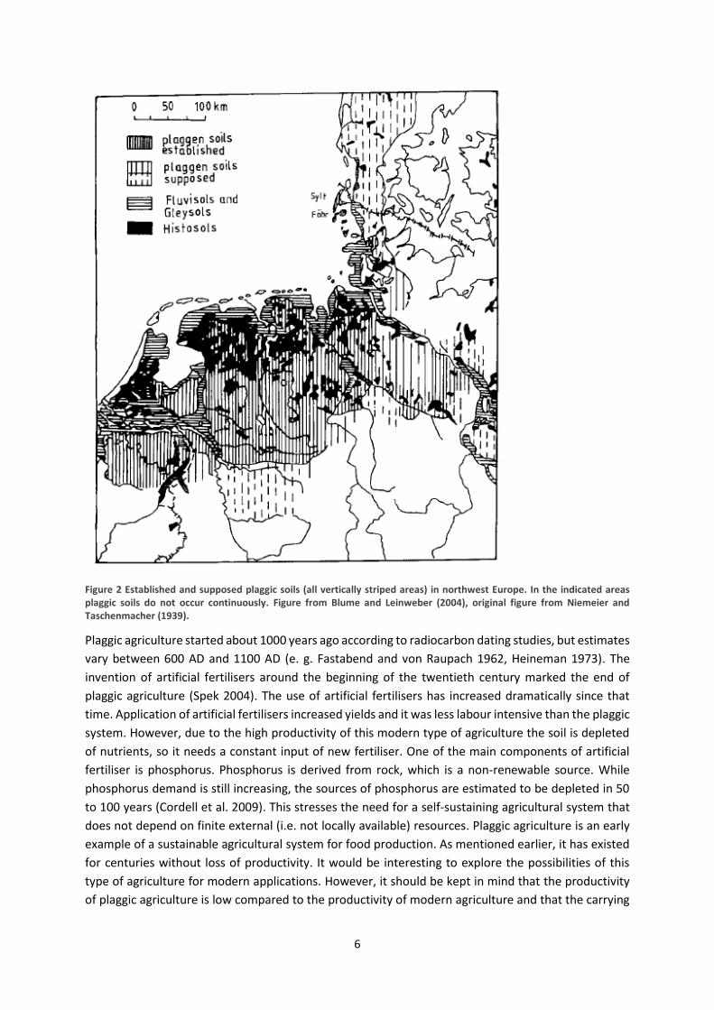
popular (Giani et al. 2014). The vertically striped area in Figure 2 is now worldwide the largest area in
which plaggic anthrosols occur discontinuously and it covers an area of around 0.5 million ha (Dudal
and Driessen 1991).
6
Figure 2 Established and supposed plaggic soils (all vertically striped areas) in northwest Europe. In the indicated areas plaggic soils do not occur continuously. Figure from Blume and Leinweber (2004), original figure from Niemeier and Taschenmacher (1939).
Plaggic agriculture started about 1000 years ago according to radiocarbon dating studies, but estimates
vary between 600 AD and 1100 AD (e. g. Fastabend and von Raupach 1962, Heineman 1973). The
invention of artificial fertilisers around the beginning of the twentieth century marked the end of
plaggic agriculture (Spek 2004). The use of artificial fertilisers has increased dramatically since that
time. Application of artificial fertilisers increased yields and it was less labour intensive than the plaggic
system. However, due to the high productivity of this modern type of agriculture the soil is depleted
of nutrients, so it needs a constant input of new fertiliser. One of the main components of artificial
fertiliser is phosphorus. Phosphorus is derived from rock, which is a non-renewable source. While
phosphorus demand is still increasing, the sources of phosphorus are estimated to be depleted in 50
to 100 years (Cordell et al. 2009). This stresses the need for a self-sustaining agricultural system that
does not depend on finite external (i.e. not locally available) resources. Plaggic agriculture is an early
example of a sustainable agricultural system for food production. As mentioned earlier, it has existed
for centuries without loss of productivity. It would be interesting to explore the possibilities of this
type of agriculture for modern applications. However, it should be kept in mind that the productivity
of plaggic agriculture is low compared to the productivity of modern agriculture and that the carrying
7
capacity of the landscape for plaggic agriculture is limited. At the peak time of plaggic agriculture in
northwest Europe the population density and thus the area needed for food production was much
smaller than it is now, but even during that time the carrying capacity of the landscape was sometimes
exceeded, resulting in drift sand activity on the locations where sods were removed from the soil
(Lungershausen et al. 2017). Using the 1:10 ratio mentioned by Niemeier and Taschenmacher (1939),
there will simply not be enough land to sustain plaggic agriculture for the present-time food demand.
It is therefore not an option to go back to these old agricultural practices, but still there might be much
we can learn from this former type of agriculture that was fully self-sustaining and productive over a
prolonged period of time. Another advantageous property of plaggic soils is that they are extremely
rich in stable organic matter, so their potential for carbon sequestration (e.g. Freibauer et al. 2004,
Merante et al. 2017) could be large. If we could return to agricultural soils that contain more organic
matter, more organic carbon is incorporated in the soil, possibly contributing to a lower carbon dioxide
level in the atmosphere. Therefore, it is important to have a proper idea of how plaggic soils were
managed. Examples of such management aspects are the soil reworking rate resulting from
bioturbation and ploughing and the accumulation rate, which is the rate of elevation of the soil surface
level due to application of plaggen sods.
The rates of accumulation and soil reworking can be derived from ages at several depths in the soil. In
the past, efforts have been made to date plaggic anthrosols using radiocarbon dating (Van Mourik et
al. 1995). A problem of this method is that the ages of carbon found in a sample do not necessarily
reflect the age of deposition. Some of the organic material in the soil may be formed in situ, while
other organic material has originated from the sods that were applied as manure (Bokhorst et al. 2005).
The origin of pollen in a sample is also uncertain. They may have been inside the applied sods as well
(Mucher et al. 1989). For these reasons, radiocarbon dating and palynological dating will not give
reliable accumulation and mixing rates. Luminescence dating does not provide the formation age of
soil material, but it dates the time since mineral grains were last exposed to daylight. This makes it
possible to determine the mixing rates and accumulation rates.
Luminescence dating of plaggic anthrosols The long and rich history of plaggic agriculture can be unravelled using luminescence dating. Using this
dating method, the age of mineral soil material can be derived from the radiation dose that the grain
has received from its surroundings during burial (called burial dose, estimated by the palaeodose). This
will be explained in detail in the background section. In contrast to laboratory experiments, which
usually do not last for more than a few years, luminescence dating can provide insight into the long-
term effects of land management on soil properties. The conventional multiple grain quartz optically
stimulated luminescence (OSL) method has already been used to date plaggic anthrosols (e. g.
Bokhorst et al. 2005, Van Mourik et al. 2011, Van Mourik et al. 2012). They used the single aliquot
regenerative dose (SAR) technique to determine the palaeodose and the age of the samples. Bokhorst
et al. (2005) found that the aliquot size was too large to determine if the luminescence signal of
individual grains was zeroed during aeolian deposition or because of ploughing activities that
transported the grain to the surface. Therefore Bokhorst et al. (2005) proposed analysis of smaller
aliquots to separate these two processes. Small-aliquot SAR has already been used by Van Mourik et
al. (2011) to determine the ages of a mineral soil matrix. They compared these ages to the radiocarbon
ages of the same sample and proved that the organic material in the spaces between mineral grains
was older than the mineral matrix.
8
Using conventional multiple grain quartz OSL measurements, the moment that the luminescence
signal started to accumulate in a grain can be dated reliably and it represents the moment that the
grain was buried below the ploughing layer. In addition, single-grain analysis potentially provides extra
information on soil processes occurring over time, such as mixing and accumulation rates. These rates
could contain information on former land use methods. For example, the reworking rate as a result of
ploughing could be derived from the dose distributions of the grains in the ploughing horizon. It is
expected that this rate was low in the early Middle Ages, so ploughing horizons of that age will contain
relatively old grains that have never surfaced due to the low ploughing intensity. When the ploughing
intensity started to increase, more grains reached the surface and thus the dose distributions of more
intensively ploughed layers are expected to be narrower. The moment at which plaggen sods started
to be added to the soil should also be visible from the dose distributions, because the addition of sods
to the soil results in a rise of the soil surface and therefore also of the lower boundary of the ploughing
horizon. Single-grain measurements are labour intensive and time consuming and only a few percent
of the quartz grains emit a luminescence signal that is bright enough for measurement. On the other
hand, several tens of percent of the feldspar grains are suitable for luminescence dating (Reimann et
al. 2012), which is an order of magnitude more than for quartz. Because many feldspar grains give a
suitable signal, the feldspar mineral is especially useful for single grain measurements. Although most
soil samples will contain more quartz than feldspar, measurement of the feldspar signal is more
efficient than measurement of the quartz signal.
9
Research objectives
This study has two objectives. On the one hand, it assesses how the feldspar single-grain dating
protocol as developed by Reimann et al. (2012) performs in determining the accumulation and
reworking rates in plaggic soils. In addition, these rates will be used to clarify the history of these soils.
This knowledge may be applied in modern agriculture to create healthy soils containing more stable
organic matter and thereby making agricultural practices more sustainable.
The accumulation and reworking rates contain much information on historical plaggic agriculture. The
effective reworking rate is defined by the speed at which the soil is reworked (sample depth divided
by apparent luminescence burial age) and the number of grains that participate in reworking (Reimann
et al. 2017). The accumulation rate is the speed at which the soil surface elevates because of plaggen
addition. Spek (2004) expresses the need for a detailed and statistically reliable dating method for
determining the ages of layers in a plaggic anthrosol to get a better impression of the accumulation
rate over time. He also states that detecting and dating vertical displacement of soil material requires
analysis of the age distribution of a large dataset rather than dating individual soil elements. Single-
grain dating provides such age distributions and feldspar is the most efficient mineral to use. For these
reasons the feldspar single-grain luminescence dating method will be used in this study.
The first appearance of plaggic agriculture is not well established yet because suitable dating methods
were lacking. Studies that determined the onset of plaggic agriculture using radiocarbon dating and
pollen analysis do not give consistent ages (Giani et al. 2014). Furthermore, these ages are not reliable
because soil organic carbon is mobile and has probably not been produced in situ and the pollen in the
soil profile may originate from other locations as well (Van Mourik et al. 2011). Luminescence dating
does not suffer from these problems. Single-grain luminescence analysis is an ideal method for
determining both the accumulation and reworking rates, since it determines the ages of plaggic
anthrosols much more reliably than radiocarbon dating and palynological analysis (Giani et al. 2014)
and it enables analysis of the age distribution within a sample. However, the relatively new feldspar
single-grain method has not yet been applied to a plaggic anthrosol nor has it been tested in this
particular setting. This study aims to establish a dating method that can provide a reliable age for the
first appearance of plaggic agriculture and its development over space and time. Furthermore, it aims
to determine the reworking rate and accumulation rate of a plaggic anthrosol in the eastern part of
the Netherlands. The single-grain feldspar ages will be compared to independent age estimates for
samples from the same location. The research questions that will be answered are:
1. When did plaggic agriculture start to develop at the location of the investigated plaggic
anthrosol according to the feldspar single-grain dating method?
2. What are the reworking rates in the plaggic soil and what is the difference between natural
and anthropogenic soil reworking?
3. What are the historical accumulation rates in the plaggic soil?
4. How does the single-grain feldspar dating method perform compared to independent
estimates including quartz OSL and field observations?
10
Background
Luminescence dating Luminescence dating is based on the principle that a latent luminescence signal builds up in a mineral
grain (quartz or feldspar) due to the ionising radiation it receives from its surroundings. When the grain
is exposed to daylight or heated to a few hundred degrees Celsius the signal is emitted. This signal can
be measured, and the luminescence age can be derived from it. Once the exposure to daylight or
heating stops, the signal will start to accumulate again. This principle allows calculation of the time
that has passed since the grain was deposited, covered by other deposits or brought to the soil surface
by reworking processes (Stockmann et al. 2013). In this study the accumulation and emission of the
luminescence signal occurs in the context of soil reworking.
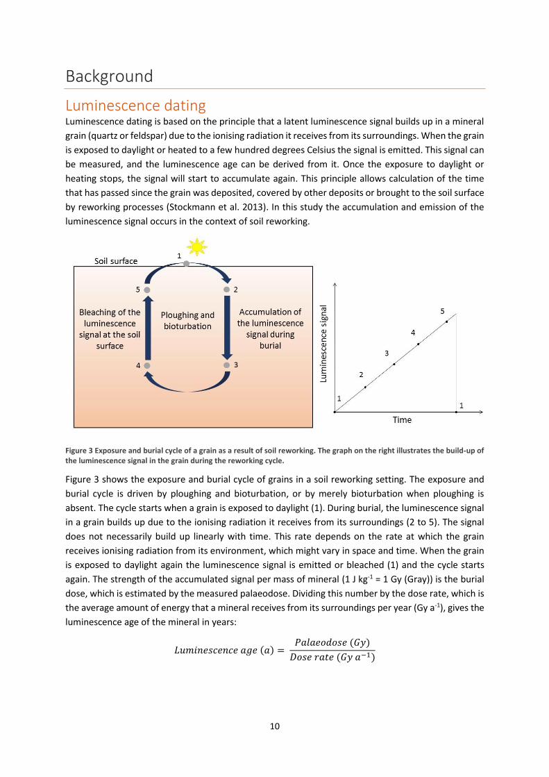
Figure 3 Exposure and burial cycle of a grain as a result of soil reworking. The graph on the right illustrates the build-up of the luminescence signal in the grain during the reworking cycle.
Figure 3 shows the exposure and burial cycle of grains in a soil reworking setting. The exposure and
burial cycle is driven by ploughing and bioturbation, or by merely bioturbation when ploughing is
absent. The cycle starts when a grain is exposed to daylight (1). During burial, the luminescence signal
in a grain builds up due to the ionising radiation it receives from its surroundings (2 to 5). The signal
does not necessarily build up linearly with time. This rate depends on the rate at which the grain
receives ionising radiation from its environment, which might vary in space and time. When the grain
is exposed to daylight again the luminescence signal is emitted or bleached (1) and the cycle starts
again. The strength of the accumulated signal per mass of mineral (1 J kg-1 = 1 Gy (Gray)) is the burial
dose, which is estimated by the measured palaeodose. Dividing this number by the dose rate, which is
the average amount of energy that a mineral receives from its surroundings per year (Gy a-1), gives the
luminescence age of the mineral in years:
𝐿𝑢𝑚𝑖𝑛𝑒𝑠𝑐𝑒𝑛𝑐𝑒 𝑎𝑔𝑒 (𝑎) = 𝑃𝑎𝑙𝑎𝑒𝑜𝑑𝑜𝑠𝑒 (𝐺𝑦)
𝐷𝑜𝑠𝑒 𝑟𝑎𝑡𝑒 (𝐺𝑦 𝑎−1)
11
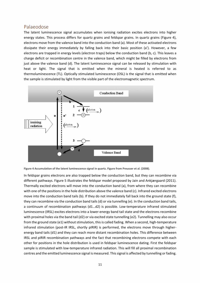
Palaeodose The latent luminescence signal accumulates when ionising radiation excites electrons into higher
energy states. This process differs for quartz grains and feldspar grains. In quartz grains (Figure 4),
electrons move from the valence band into the conduction band (a). Most of these activated electrons
dissipate their energy immediately by falling back into their basic position (a’). However, a few
electrons are trapped in energy levels (electron traps) below the conduction band (b, c). This leaves a
charge deficit or recombination centre in the valence band, which might be filled by electrons from
just above the valence band (d). The latent luminescence signal can be released by stimulation with
heat or light. The signal that is emitted when the mineral is heated is referred to as
thermoluminescence (TL). Optically stimulated luminescence (OSL) is the signal that is emitted when
the sample is stimulated by light from the visible part of the electromagnetic spectrum.
Figure 4 Accumulation of the latent luminescence signal in quartz. Figure from Preusser et al. (2008).
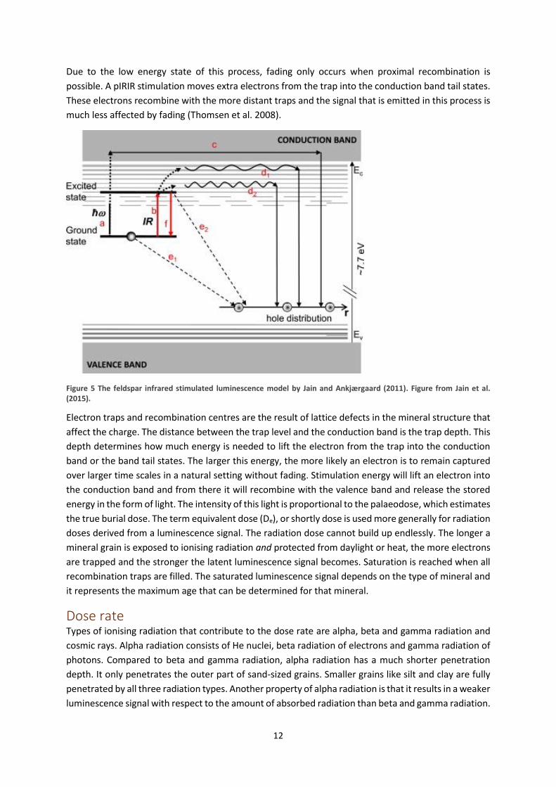
In feldspar grains electrons are also trapped below the conduction band, but they can recombine via
different pathways. Figure 5 illustrates the feldspar model proposed by Jain and Ankjærgaard (2011).
Thermally excited electrons will move into the conduction band (a), from where they can recombine
with one of the positions in the hole distribution above the valence band (c). Infrared excited electrons
move into the conduction band tails (b). If they do not immediately fall back into the ground state (f),
they can recombine via the conduction band tails (d) or via tunnelling (e). In the conduction band tails,
a continuum of recombination pathways (d1…d2) is possible. Low-temperature infrared stimulated
luminescence (IRSL) excites electrons into a lower-energy band tail state and the electrons recombine
with proximal holes via the band tail (d2) or via excited state tunnelling (e2). Tunnelling may also occur
from the ground state (e1) without stimulation, this is called fading. When a second, high-temperature
infrared stimulation (post-IR IRSL, shortly pIRIR) is performed, the electrons move through higher-
energy band tails (d1) and they can reach more distant recombination holes. This difference between
IRSL and pIRIR recombination pathways and the fact that recombining electrons compete with each
other for positions in the hole distribution is used in feldspar luminescence dating. First the feldspar
sample is stimulated with low-temperature infrared radiation. This will fill all proximal recombination
centres and the emitted luminescence signal is measured. This signal is affected by tunnelling or fading.
12
Due to the low energy state of this process, fading only occurs when proximal recombination is
possible. A pIRIR stimulation moves extra electrons from the trap into the conduction band tail states.
These electrons recombine with the more distant traps and the signal that is emitted in this process is
much less affected by fading (Thomsen et al. 2008).
Figure 5 The feldspar infrared stimulated luminescence model by Jain and Ankjærgaard (2011). Figure from Jain et al. (2015).
Electron traps and recombination centres are the result of lattice defects in the mineral structure that
affect the charge. The distance between the trap level and the conduction band is the trap depth. This
depth determines how much energy is needed to lift the electron from the trap into the conduction
band or the band tail states. The larger this energy, the more likely an electron is to remain captured
over larger time scales in a natural setting without fading. Stimulation energy will lift an electron into
the conduction band and from there it will recombine with the valence band and release the stored
energy in the form of light. The intensity of this light is proportional to the palaeodose, which estimates
the true burial dose. The term equivalent dose (De), or shortly dose is used more generally for radiation
doses derived from a luminescence signal. The radiation dose cannot build up endlessly. The longer a
mineral grain is exposed to ionising radiation and protected from daylight or heat, the more electrons
are trapped and the stronger the latent luminescence signal becomes. Saturation is reached when all
recombination traps are filled. The saturated luminescence signal depends on the type of mineral and
it represents the maximum age that can be determined for that mineral.
Dose rate Types of ionising radiation that contribute to the dose rate are alpha, beta and gamma radiation and
cosmic rays. Alpha radiation consists of He nuclei, beta radiation of electrons and gamma radiation of
photons. Compared to beta and gamma radiation, alpha radiation has a much shorter penetration
depth. It only penetrates the outer part of sand-sized grains. Smaller grains like silt and clay are fully
penetrated by all three radiation types. Another property of alpha radiation is that it results in a weaker
luminescence signal with respect to the amount of absorbed radiation than beta and gamma radiation.
13
The environmental dose rate that is needed for luminescence age calculation is the sum of internal
radiation, external radiation and cosmic radiation. Internal radiation is produced within the mineral
grain itself. The most important source of internal radiation is 40K, which is present in alkali feldspars
but not in quartz. For that reason, internal radiation is often neglected for quartz but not for feldspar.
External radiation is the radiation that a mineral grain receives from the surroundings. It mainly
originates from the 238U/235U and 232Th decay chains and from 40K in feldspars, micas and clay minerals.
Other radioactive elements in the surroundings generally contribute very little to the external
radiation, so they are neglected. An important factor to consider in external dose rate calculations is
the moisture content of the sediment, because moisture attenuates the radiation coming from
surrounding grains much more than air. Cosmic radiation consists of particles from outside our solar
system that penetrate the Earth surface. The Earth magnetic field causes the intensity of cosmic
radiation to be larger near the poles and the amount of cosmic radiation absorbed by a mineral grain
decreases with increasing water and sediment overburden.
Measuring soil mixing using single-grain luminescence Conventional multiple grain luminescence dating is based on the assumption that post-depositional
mixing is absent or negligible. Mixing of the profile used to be an obstacle for age determination and
process interpretation. When single-grain analysis was developed, it was a tool to ‘correct’ for
bioturbation processes. Lately it has been used to study the mixing processes themselves (e.g.
Kristensen et al. 2015, Gliganic et al. 2016). Single-grain luminescence is especially relevant for soils,
because soils are subjected to mixing, whereas conventional multiple grain luminescence is used for
unmixed layered sediments. When luminescence dating is performed on single grains, the dose
distribution of the grains in one sample reveals the ages of grains present at one location. Soil mixing
rates can be estimated from the equivalent dose distribution in a certain sample (Figure 6) (Bateman
et al. 2003).
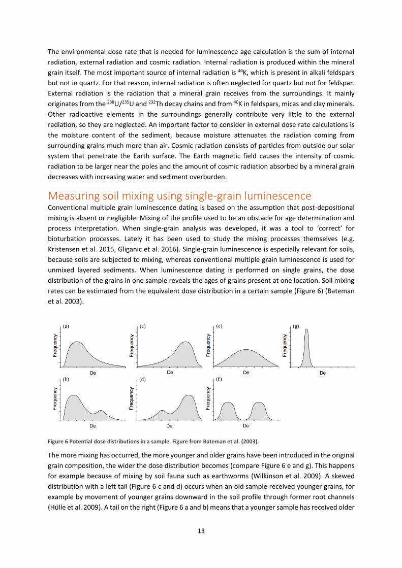
Figure 6 Potential dose distributions in a sample. Figure from Bateman et al. (2003).
The more mixing has occurred, the more younger and older grains have been introduced in the original
grain composition, the wider the dose distribution becomes (compare Figure 6 e and g). This happens
for example because of mixing by soil fauna such as earthworms (Wilkinson et al. 2009). A skewed
distribution with a left tail (Figure 6 c and d) occurs when an old sample received younger grains, for
example by movement of younger grains downward in the soil profile through former root channels
(Hülle et al. 2009). A tail on the right (Figure 6 a and b) means that a younger sample has received older
14
grains. Skewed distributions are normally the result of minor mixing processes whereas a wide normal
distribution is the result of intensive mixing (Bateman et al. 2003). A multi-modal distribution (Figure
6 b, d and f) reflects separated phases of mixing. In that case, only one peak will refer to the age of
deposition, the other peaks are related to the mixing phases and represent the ages of the material
that is mixed into the sample (Bateman et al. 2003).
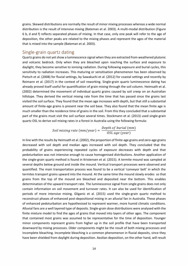
Single-grain quartz dating Quartz grains do not yet show a luminescence signal when they are extracted from weathered plutonic
and volcanic bedrock. Only when they are bleached upon reaching the surface and exposure to
daylight, they become sensitive to ionising radiation. During following exposure and burial cycles, this
sensitivity to radiation increases. This maturing or sensitisation phenomenon has been observed by
Pietsch et al. (2008) for fluvial settings, by Sawakuchi et al. (2012) for coastal settings and recently by
Reimann et al. (2017) in the context of soil reworking. Single-grain quartz luminescence dating has
already proved itself useful for quantification of grain mixing through the soil column. Heimsath et al.
(2002) determined the movement of individual quartz grains caused by soil creep on an Australian
hillslope. They derived the vertical mixing rate from the time that has passed since the grains last
visited the soil surface. They found that the mean age increases with depth, but that still a substantial
amount of finite-age grains is present near the soil base. They also found that the mean finite age is
much smaller than the residence time of grains in the soil. From this they concluded that a substantial
part of the grains must visit the soil surface several times. Stockmann et al. (2013) used single-grain
quartz OSL to derive soil mixing rates in a forest in Australia using the following formula:
𝑆𝑜𝑖𝑙 𝑚𝑖𝑥𝑖𝑛𝑔 𝑟𝑎𝑡𝑒 (𝑚𝑚/𝑦𝑒𝑎𝑟) = 𝐷𝑒𝑝𝑡ℎ 𝑜𝑓 𝑏𝑢𝑟𝑖𝑎𝑙 (𝑚𝑚)
𝑂𝑆𝐿 𝑎𝑔𝑒 (𝑦𝑒𝑎𝑟)
In line with the results by Heimsath et al. (2002), the proportion of finite-age grains and zero-age grains
decreased with soil depth and median ages increased with soil depth. They concluded that the
probability of grains experiencing repeated cycles of exposure decreases with depth and that
pedoturbation was not intensive enough to cause homogenised distributions. Another application of
the single-grain quartz method is found in Kristensen et al. (2015). A termite mound was sampled at
several depths below ground and inside the mound. Vertical transport processes were observed and
quantified. The main transportation process was found to be a vertical ‘conveyor belt’ in which the
termites transport grains upward into the mound. At the same time the mound slowly erodes so that
grains from the top of the mound are bleached and deposited near the bottom. This enables
determination of the upward transport rate. The luminescence signal from single grains does not only
contain information on soil movement and turnover rates. It can also be used for identification of
periods of more intensive mixing. Gliganic et al. (2015) used the single-grain quartz method to
reconstruct phases of enhanced post-depositional mixing in an alluvial fan in Australia. These phases
of enhanced pedoturbation are hypothesised to represent warmer, more humid climatic conditions.
Alluvial fans are a well layered type of deposits. Single-grain dose distributions were analysed with the
finite mixture model to find the ages of grains that moved into layers of other ages. The component
that contained most grains was assumed to be representative for the time of deposition. Younger
minor components represent grains from higher up in the soil profile that have been transported
downward by mixing processes. Older components might be the result of both mixing processes and
incomplete bleaching. Incomplete bleaching is a common phenomenon in fluvial deposits, since they
have been shielded from daylight during deposition. Aeolian deposition, on the other hand, will result
15
in complete bleaching. Phases of aeolian dune aggradation and subsequent modern mixing processes
were identified and modelled by Gliganic et al. (2016). Their soil profile consisted of layered aeolian
deposits that were mixed by subsequent bioturbation. This mixing was so strong that the depositional
ages could not be determined, because the finite mixture model did not give reliable ages. A
combination of the minimum age model and a mixing zone model resulted in the identification of three
mixing phases.
Single-grain feldspar dating Until now single-grain luminescence dating has been mainly applied to quartz grains (e. g. Heimsath et
al. 2002, Stockmann et al. 2013, Gliganic et al. 2015, Kristensen et al. 2015, Gliganic et al. 2016). These
studies are often performed in areas where quartz grains show exceptionally good luminescence
properties (e. g. Heimsath et al. 2002, Stockmann et al. 2013). The luminescence signal of quartz grains
from Australia, for example, is a few orders of magnitude brighter than that of European quartz grains
(Pietsch et al. 2008), which is considerably more convenient for measurements. However, in most
cases the single-grain quartz OSL method is time consuming and labour intensive as only 1 to 5 % of
the quartz grains have a luminescence signal that is bright enough for accurate measurement (e. g.
Duller 2008, Demuro et al. 2013). An additional disadvantage of the single-grain quartz method are the
sensitivity changes resulting from repeated exposure and burial cycles (Murray and Roberts 1998).
A more widely applicable single-grain method was recently proposed by Reimann et al. (2017). They
used individual sand-sized feldspar grains as soil reworking tracers to reconstruct soil reworking rates
for a soil profile in Spain. The advantages of this method over the single-grain quartz method are that
many feldspar grains emit a suitable luminescence signal, also if they have never been exposed to
daylight (Duller 2006, Reimann et al. 2012), that the luminescence signal of feldspar grains does not
depend on the number of exposure and burial cycles that it has experienced (Lukas et al. 2007), and
that a large fraction of the environmental dose rate originates from 40K inside the feldspar grain, which
minimises the inaccuracies arising from the assumption that the external radiation field was constant
over the entire burial time (e. g. Reimann et al. 2011). A disadvantage is that feldspar IRSL signals are
subject to anomalous fading (Spooner 1994), which means that trapped electrons in the ground state
slowly recombine to less energetic levels near the valence band through tunnelling, leading to
measurement of a weaker luminescence signal and thus to age underestimation. Another
disadvantage of using feldspar grains to determine soil reworking rates is that feldspar grains need a
longer daylight exposure time than quartz grains to bleach completely because the bleaching rate is
slower (Godfrey-Smith et al. 1988). This effect is stronger for pIRIR signals than for the IRSL signals
(Godfrey-Smith et al. 1988, Murray et al. 2012). This increases the probability of incomplete bleaching
and thus of age overestimation. The method by Reimann et al. (2017) minimises both disadvantages.
Low-temperature (< 200 °C) IRSL and pIRIR feldspar signals are used, because they are better
bleachable than high-temperature signals (Kars et al. 2014). This low temperature pIRIR signal is also
less sensitive to anomalous fading according to Reimann et al. (2011).
Secondly, they propose a novel way to calculate the soil reworking rate. Until now, calculations of the
soil reworking rate as used by e. g. Stockmann et al. (2013) did not consider the proportion of mineral
grains that never reached the surface. They determined the reworking rate from the grains that
showed a suitable luminescence signal only. Reimann et al. (2017) argue that this is only an apparent
reworking rate (SRapp), as it does not take into account the depth dependency of soil reworking. They
introduced the non-saturation factor (NSF), the proportion of non-saturated grains to the total number
16
of grains that were used in the analysis, to correct for the grains not participating in reworking (the so-
called ‘out of competition’ grains with a reworking rate of 0 mm y-1). The apparent reworking rate
multiplied by the NSF gives the effective soil reworking rate (SReff), which is dependent on depth. The
more grains are out of competition, the smaller the effective reworking rate is compared to the
apparent reworking rate. The results of the feldspar single-grain method were compared to the results
of the more conventional quartz single-grain method. The feldspar SReff is dependent on depth,
whereas the quartz SReff is similar for each of the upper three samples but much lower for the lowest
sample. Because quartz grains recently derived from weathered bedrock mature and sensitise during
the repeated cycles of exposure and burial, the quartz grains that do not show a suitable luminescence
signal are the weathered bedrock grains that have not been reworked. This gives a bias in the SReff
estimated from quartz. The feldspar luminescence signal does not change over time, so the feldspar-
SReff are a better estimate of the reworking rate than the quartz-SReff.
Analysis of single-grain distributions Apart from the type of mixing process that can be derived from the shape of a single-grain distribution
(Figure 6), there is often a need for quantitative information. In most cases this includes the palaeodose
of one or more peaks in a sample distribution. Statistical age models have been developed to identify
these peaks. The most commonly used ones are discussed below. The choice for an age model must
always be made considering prior knowledge of a sample, such as the sedimentary context and the
bleaching state that is expected based on for example the depositional environment. The different
single-grain dose distributions in Figure 6 require different methods of analysis, depending on the type
of distribution and the type of age (minimum age, maximum age, etc.) that needs to be derived. Age
models are usually applied to the log-transformed equivalent dose measurements, because their
errors are symmetrically distributed. This log-transformation requires that the equivalent dose dataset
exclusively consists of positive estimates. However, for samples containing near-zero aged grains some
measurements will give negative equivalent dose values. The age models can also be applied to the
unlogged equivalent dose measurements, but for samples older than approximately 350 years this may
lead to underestimation of the burial age (Arnold et al. 2009). Age models can be bootstrapped, which
means that they measure the statistical properties (e.g. age and spread in the age distribution) of a
sample by taking subsets from the sample and determining the average statistical properties for these
subsets. This allows for inferences about statistical properties of the population from measurements
on the sample, because the relation between a sample subset and a sample is assumed to be the same
as the relation between a population and a sample (Efron and Tibshirani 1993, Cunningham and
Wallinga 2012).
In addition to the age, the spread in a single-grain De distribution is often assessed. This spread has
several sources. Experimental errors are the errors of the combined measurements (counting
statistics), the Monte Carlo fitting error and the error of the measurement equipment. The spread in
the equivalent dose distribution that is not explained by these experimental errors is called the
overdispersion. The overdispersion can partially be explained by variations in natural circumstances
like mixing and poor bleaching, but even for a sample that is known not to be mixed after deposition
and for which deposition has occurred instantaneously and after complete bleaching, still a certain
amount of overdispersion is present. This is called the minimum overdispersion σb. One of the sources
of this minimum overdispersion is for example a spatially and temporally heterogeneous dose rate in
the radiation field (Olley et al. 1997).
17
Weighted mean age models When the single-grain De distribution is normally distributed with only a few outliers, the age of interest
is often the mean age. In the calculation of the mean De the errors of the individual measurements are
used as a weighting factor. An error-weighted mean age reduces the influence of grains having a large
dose measurement error and gives more weight to grains of which the equivalent dose was
determined more precisely. There are two types of weighted mean age models. The common age
model determines the weighted mean as a single value without standard error whereas the central
age model (CAM) determines the weighted mean as a normal distribution of ages (Galbraith et al.
1999). The latter is more often used for luminescence dating purposes.
Minimum age model and maximum age model The minimum age model of Galbraith et al. (1999) estimates the equivalent dose corresponding to the
youngest, leading-edge population in a sample distribution. This model is often applied to fluvial
samples, because fluvially deposited grains are often not completely bleached before burial (e. g.
Arnold et al. 2007, Pietsch et al. 2008). As described in (Galbraith and Roberts 2012), the minimum age
model fits a truncated normal distribution to the logged equivalent dose values. The lower truncation
point is assumed to correspond to the average dose of the leading-edge population. In the four-
parameter minimum age model (MAM-4), the lower truncation point γ is smaller than the mean of the
normal distribution µ. The other two parameters of this model are the standard deviation σ and the
proportion of fully bleached grains p. When the lower truncation point coincides with the mean of the
normal distribution (γ =µ), the model contains only three parameters (MAM-3). This three-parameter
model is more commonly used than the four-parameter model.
The maximum age model is essentially an inversion of the minimum age model by Galbraith et al.
(1999). Instead of determining the dose of the youngest subpopulation, it determines the dose of the
oldest subpopulation. All parameters are the same, except that γ is now defined as the upper
truncation point. This model can be used when the age of interest corresponds to the maximum peak
in the single-grain dose distribution. This might be a situation in which the age of older grains mixed
into a sample needs to be determined or when the burial age must be derived from a sample that has
been mixed and bleached by bioturbation.
Finite mixture model When prior knowledge on a sample setting indicates that a sample contains more than one dose
population, the finite mixture model (FMM) can be used to identify the separate populations. This
model fits several normal distributions to the sample distribution. Each fitted distribution accounts for
one population. If the number of subpopulations is known, the finite mixture model can be applied
directly specifying the number of components. However, sometimes the number of subpopulations is
not known exactly. In that case, the number of components needs to be estimated first. The FMM can
not only be used to identify the average equivalent dose and proportion of each subpopulation, it can
also estimate the number of subpopulations. The finite mixture model can be run multiple times for
different numbers of components and the outputs of each of these runs can be compared based on
their BIC value (Bayes Information Criterion, (Schwarz 1978)). The lower this number, the better the
combined fit of the components. The number of components that results in the lowest BIC-value is
then the best estimate for the number of subpopulations in a sample population. The minimum
overdispersion of the normal distributions that are fitted to the sample distribution must be specified
in advance. It is important to know the overdispersion accurately, especially when estimating the

18
number of components, because they are closely coupled. The finite mixture model assumes all
components to have the same overdispersion. In a lot of cases this assumption may not be true, for
example when the components in a sample do not have the same sedimentary history, or when one
component is the result of post-depositional mixing whereas the other component consists of unmixed
grains. Because the finite mixture model identifies all peaks in a sample distribution, it can be used to
estimate the maximum and minimum components as well. An advantage of the FMM over the
minimum and maximum age model is that it also calculates the proportion of grains in each
component. A disadvantage of calculating these ages with the FMM is that the estimates for the
component of interest are dependent of the estimates of the remaining components, because the
proportions of all components must add up to one.
19
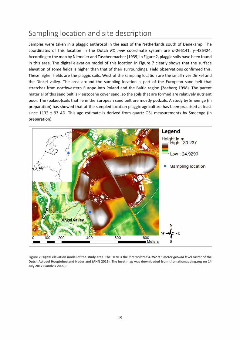
Sampling location and site description Samples were taken in a plaggic anthrosol in the east of the Netherlands south of Denekamp. The
coordinates of this location in the Dutch RD new coordinate system are x=266141, y=486424.
According to the map by Niemeier and Taschenmacher (1939) in Figure 2, plaggic soils have been found
in this area. The digital elevation model of this location in Figure 7 clearly shows that the surface
elevation of some fields is higher than that of their surroundings. Field observations confirmed this.
These higher fields are the plaggic soils. West of the sampling location are the small river Dinkel and
the Dinkel valley. The area around the sampling location is part of the European sand belt that
stretches from northwestern Europe into Poland and the Baltic region (Zeeberg 1998). The parent
material of this sand belt is Pleistocene cover sand, so the soils that are formed are relatively nutrient
poor. The (palaeo)soils that lie in the European sand belt are mostly podzols. A study by Smeenge (in
preparation) has showed that at the sampled location plaggic agriculture has been practised at least
since 1132 ± 93 AD. This age estimate is derived from quartz OSL measurements by Smeenge (in
preparation).
Figure 7 Digital elevation model of the study area. The DEM is the interpolated AHN2 0.5 meter ground level raster of the Dutch Actueel Hoogtebestand Nederland (AHN 2012). The inset map was downloaded from thematicmapping.org on 14 July 2017 (Sandvik 2009).
Dinkel valley
20
Experimental methods and details
Soil description and classification
A soil pit was dug and the soil horizons and their Munsell colour were determined (Table 1). At all
depths, the texture was classified as weakly loamy sand with a median grain size of 210 µm. The plaggic
layer consists of two Aap horizons that differ from each other in colour (Figure 8). The Aap1 horizon is
darker than the Aap2 horizon, which could indicate that different plaggen types were used. The light
colour of the Aap2 horizon might be derived from forest or heather plaggen while the darker colour
might be derived from peat plaggen, possibly taken from the lower lying Dinkel valley. A transition
horizon separates these plaggic layers. This transition horizon has an intermediate colour and in
addition brown and lighter coloured spots were observed. As a result of ploughing this transition
horizon is rather thick with indistinct upper and lower boundaries. Below the plaggic horizons a non-
plaggic light coloured ploughing layer was identified. The light colour of this layer is partly caused by
the presence of grey coloured grains that strongly resemble the grey grains normally found in the
eluviation horizon of a podzol. The unploughed part of the soil consists of a brown weathering horizon
(Bw) and cover sand parent material in which gleyic phenomena were observed (Cg). The thick plaggic
layer and the human influence on this soil are the main reasons that this soil was classified as a plaggic
anthrosol.
Table 1 Soil horizon descriptions at the sampled location.
Depth (cm) Horizon Munsell colour Remarks
0-30 Aap1 10YR 2/2 Small pieces of brick 30-50 Aap1/Aap2 10YR 3/2 Small pieces of brick, brown and lighter coloured spots 50-105 Aap2 10YR 3/3 Black spots up to ± 80 cm depth 105-120 Ap 10YR 4/2 Podzol-grey coloured grains present 120-130 Bw 10YR 4/3.5 130-170 Cg 2.5Y 5/4 Some fossil gley mottles of several cm in size present
at 150-160 cm depth.
The soil that was present at this location before the start of plaggic agriculture consists of Ap, Bw and
Cg horizons. It is clear that the original soil was not a classical poor podzol, because no eluviation (E)
and Bh horizons were found. The Bw horizon indicates that the original soil was a brown forest soil,
but the presence of podzol-grey coloured grains seems contradictory. The richness in organic matter
of the Ap horizon and the gleyic mottles in the Cg horizon do not support poor podzols. There are
several possible explanations for the presence of podzol grains in the Ap horizon. It could be that a thin
podzol was already present at this location before it started to be used for agriculture. This podzol
must have been so thin that is was completely mixed by ploughing. However, it is not very likely that
a podzol in cover sand of Pleistocene age was thin, given the long development time. Maybe the grey
grains indicate that the original brown forest soil was already degrading towards a poor podzol. The
grey grains are not necessarily formed in situ. They may also have been included in the earliest applied
plaggen sods cut from a podzol topsoil and then mixed through the ploughing horizon. Another
possibility is that the grey grains have originated from a nearby podzol and were deposited by the wind
during a period of drift sand activity. If the grey grains originate from elsewhere, whether by plaggen
application or by aeolian deposition, no palaeo-podzol has been present at this location. If the grey
grains have been formed by soil degradation, no fully developed palaeo-podzol has been present
either. Therefore, the original soil below the plaggic layers is assumed to be a brown forest soil.
21
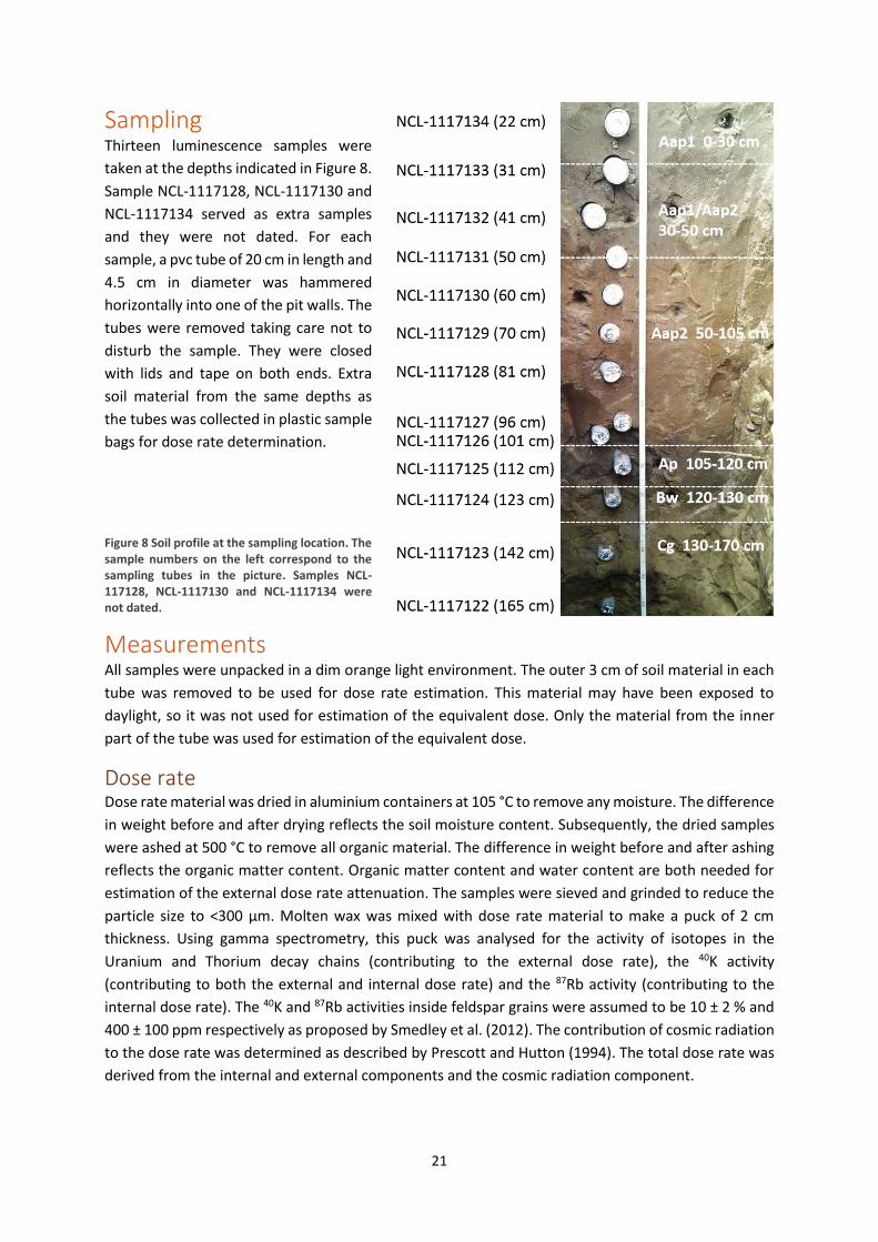
Sampling Thirteen luminescence samples were
taken at the depths indicated in Figure 8.
Sample NCL-1117128, NCL-1117130 and
NCL-1117134 served as extra samples
and they were not dated. For each
sample, a pvc tube of 20 cm in length and
4.5 cm in diameter was hammered
horizontally into one of the pit walls. The
tubes were removed taking care not to
disturb the sample. They were closed
with lids and tape on both ends. Extra
soil material from the same depths as
the tubes was collected in plastic sample
bags for dose rate determination.
Figure 8 Soil profile at the sampling location. The sample numbers on the left correspond to the sampling tubes in the picture. Samples NCL-117128, NCL-1117130 and NCL-1117134 were not dated.
Measurements All samples were unpacked in a dim orange light environment. The outer 3 cm of soil material in each
tube was removed to be used for dose rate estimation. This material may have been exposed to
daylight, so it was not used for estimation of the equivalent dose. Only the material from the inner
part of the tube was used for estimation of the equivalent dose.
Dose rate Dose rate material was dried in aluminium containers at 105 °C to remove any moisture. The difference
in weight before and after drying reflects the soil moisture content. Subsequently, the dried samples
were ashed at 500 °C to remove all organic material. The difference in weight before and after ashing
reflects the organic matter content. Organic matter content and water content are both needed for
estimation of the external dose rate attenuation. The samples were sieved and grinded to reduce the
particle size to <300 µm. Molten wax was mixed with dose rate material to make a puck of 2 cm
thickness. Using gamma spectrometry, this puck was analysed for the activity of isotopes in the
Uranium and Thorium decay chains (contributing to the external dose rate), the 40K activity
(contributing to both the external and internal dose rate) and the 87Rb activity (contributing to the
internal dose rate). The 40K and 87Rb activities inside feldspar grains were assumed to be 10 ± 2 % and
400 ± 100 ppm respectively as proposed by Smedley et al. (2012). The contribution of cosmic radiation
to the dose rate was determined as described by Prescott and Hutton (1994). The total dose rate was
derived from the internal and external components and the cosmic radiation component.
22
Equivalent dose The inner material from the tubes was used for measurement of the equivalent dose. Approximately
100 grams of soil material from each sample were weighed in a beaker, mixed with water and sieved
to separate the size fractions <212 µm, 212-250 µm and >250 µm. After sieving, the size fraction 212-
250 µm was cleaned by magnetic separation. This removes all magnetic particles, so that the remaining
grains are mainly quartz and feldspar and some other non-magnetic minerals. Further cleaning
consisted of adding an excess of 10% HCl to remove calcium carbonates and an excess of 10% H2O2 to
remove organic material. For luminescence measurements, organic material must not be removed by
ashing, because the elevated temperature will affect the luminescence signal of the grains. K-feldspar
grains having a density of 2.57 g/cm3 were separated from the quartz grains (2.64 g/cm3) and the
heavier Ca and Na feldspars by density separation using LST heavy liquid of 2.58 g/cm3.
The luminescence signal of the feldspar grains was measured using an automated Risø TL/OSL reader
(DA 15) fitted with a red and green laser single-grain attachment. The grains were stimulated for 1.68
s with a 150 mW 830 nm IR laser. All feldspar grains were detected through a LOT/Oriel D410/30
interference filter to select the K-rich feldspar emission around 410 nm. For dose-response
measurements a 90Sr/90Y beta source irradiated the samples at a dose rate of 0.1145 Gy/s. For single-
grain measurements aluminium single-grain discs with a 10x10 grid of 300 µm grain holes were used
to ensure that exactly one feldspar grain of size 212-250 µm fits in one hole.
First the rough equivalent dose of the samples was estimated with multiple grain De measurements.
The equivalent dose estimates were used to optimise the single-grain equivalent dose measurement
protocol. To test the performance of the measurement protocol, a single-grain dose recovery test was
performed on samples NCL-1117123 and NCL-1117129. Two components of the feldspar luminescence
signal were measured: first the infrared stimulated luminescence signal at 50°C (IRSL50) and then the
post-infrared signal at 175°C (pIRIR175). The samples were bleached in a solar simulator for 45 hours,
receiving simulated daylight five times as strong as natural daylight. The remaining signal was
measured as the laboratory residual dose. Subsequently dose recovery measurements were
performed, and the laboratory residual dose was subtracted from the recovered doses. This yielded
the dose recovery ratios in Table 2.
Table 2 Dose recovery ratios for the IRSL and pIRIR signal of sample NCL-1117123 and NCL-1117129. The number of grains used for residual dose measurement (nres) and dose recovery measurement (nDR) are indicated between brackets for each dose recovery ratio.
Sample pIRIR IRSL
NCL-1117123 0.97 ± 0.04 (nres = 15, nDR = 81) 1.00 ± 0.03 (nres = 54, nDR = 106) NCL-1117129 0.99 ± 0.05 (nres = 23, nDR = 24) 0.92 ± 0.04 (nres = 6, nDR = 22)
Three of the four ratios are consistent with 1 within 1σ. The dose recovery ratio of the IRSL signal for
sample NCL-1117129 is a bit low. This value is based on a small number of grains, which might explain
why this value differs from the other values. However, the value still is consistent with 1 within 2σ. The
equivalent dose measurements of the natural signal and the laboratory doses were performed using a
low pre-heat of 200°C for 120 s, an infrared stimulation at 50°C for 1.68 s, a pIRIR stimulation at 175°C
for 1.68 s and a cut-heat of 210 °C for 40.0s. Table 3 shows the steps of this protocol.
23
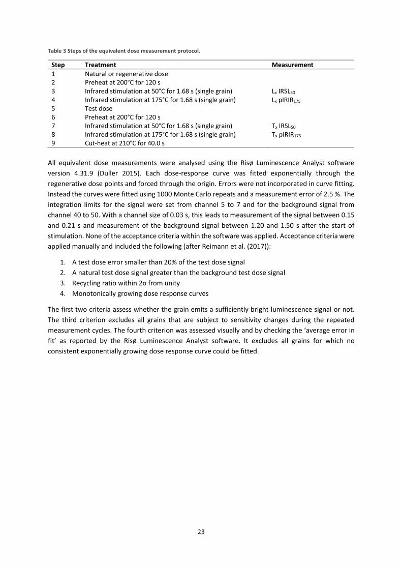
Table 3 Steps of the equivalent dose measurement protocol.
Step Treatment Measurement
1 Natural or regenerative dose 2 Preheat at 200°C for 120 s 3 Infrared stimulation at 50°C for 1.68 s (single grain) Lx IRSL50 4 Infrared stimulation at 175°C for 1.68 s (single grain) Lx pIRIR175 5 Test dose 6 Preheat at 200°C for 120 s 7 Infrared stimulation at 50°C for 1.68 s (single grain) Tx IRSL50 8 Infrared stimulation at 175°C for 1.68 s (single grain) Tx pIRIR175 9 Cut-heat at 210°C for 40.0 s
All equivalent dose measurements were analysed using the Risø Luminescence Analyst software
version 4.31.9 (Duller 2015). Each dose-response curve was fitted exponentially through the
regenerative dose points and forced through the origin. Errors were not incorporated in curve fitting.
Instead the curves were fitted using 1000 Monte Carlo repeats and a measurement error of 2.5 %. The
integration limits for the signal were set from channel 5 to 7 and for the background signal from
channel 40 to 50. With a channel size of 0.03 s, this leads to measurement of the signal between 0.15
and 0.21 s and measurement of the background signal between 1.20 and 1.50 s after the start of
stimulation. None of the acceptance criteria within the software was applied. Acceptance criteria were
applied manually and included the following (after Reimann et al. (2017)):
1. A test dose error smaller than 20% of the test dose signal
2. A natural test dose signal greater than the background test dose signal
3. Recycling ratio within 2σ from unity
4. Monotonically growing dose response curves
The first two criteria assess whether the grain emits a sufficiently bright luminescence signal or not.
The third criterion excludes all grains that are subject to sensitivity changes during the repeated
measurement cycles. The fourth criterion was assessed visually and by checking the ‘average error in
fit’ as reported by the Risø Luminescence Analyst software. It excludes all grains for which no
consistent exponentially growing dose response curve could be fitted.
24
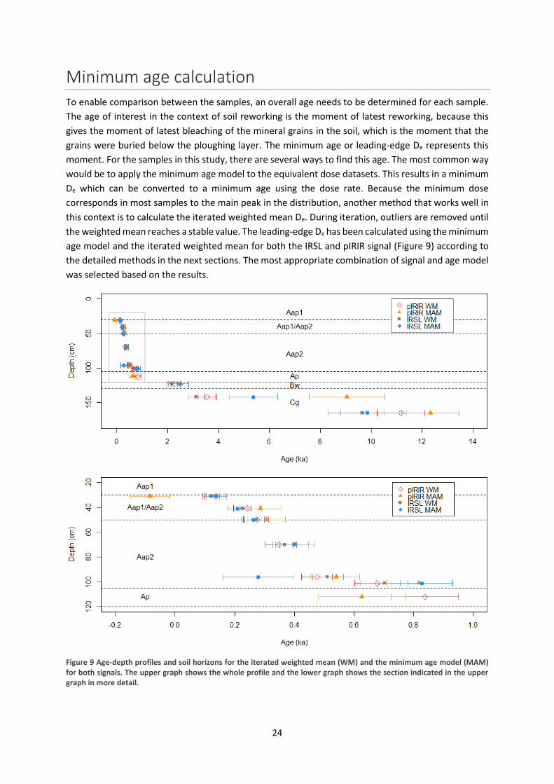
Minimum age calculation To enable comparison between the samples, an overall age needs to be determined for each sample.
The age of interest in the context of soil reworking is the moment of latest reworking, because this
gives the moment of latest bleaching of the mineral grains in the soil, which is the moment that the
grains were buried below the ploughing layer. The minimum age or leading-edge De represents this
moment. For the samples in this study, there are several ways to find this age. The most common way
would be to apply the minimum age model to the equivalent dose datasets. This results in a minimum
De which can be converted to a minimum age using the dose rate. Because the minimum dose
corresponds in most samples to the main peak in the distribution, another method that works well in
this context is to calculate the iterated weighted mean De. During iteration, outliers are removed until
the weighted mean reaches a stable value. The leading-edge De has been calculated using the minimum
age model and the iterated weighted mean for both the IRSL and pIRIR signal (Figure 9) according to
the detailed methods in the next sections. The most appropriate combination of signal and age model
was selected based on the results.
Figure 9 Age-depth profiles and soil horizons for the iterated weighted mean (WM) and the minimum age model (MAM) for both signals. The upper graph shows the whole profile and the lower graph shows the section indicated in the upper graph in more detail.
25
Minimum age model The equivalent dose datasets were loaded in Matlab (version R2017b) and the overdispersion for both
the IRSL and pIRIR signal of each sample was calculated using the bootstrapped central age model
(Cunningham and Wallinga 2012) of Galbraith et al. (1999). These overdispersion values per sample
can be found in Appendix Table 6. Subsequently the minimum overdispersion values per signal (σb)
were found by applying the bootstrapped three-parameter minimum age model (Galbraith et al. 1999,
Cunningham and Wallinga 2012) to the sample overdispersion values. The minimum overdispersion
was found to be 33 ± 4 % for the IRSL signal and 43 ± 2 % for the pIRIR signal. The bootstrapped three-
parameter minimum age model (Galbraith et al. 1999, Cunningham and Wallinga 2012) was then
applied to the De datasets using the minimum overdispersion as input to find the MAM De values
(Appendix Table 7). For some of the samples, the conventional, logged version of the model could not
be applied because of negative De values present in the dataset. For these samples the unlogged
version of the model was used. The MAM De values were converted into a MAM age using the dose
rate and then corrected for fading of the feldspar signal using the function calc_FadingCorr in the R
package Luminescence with tc (time in seconds between irradiation and the prompt measurement) set
to 2592000 s, tc.g_value (time in seconds between irradiation and the prompt measurement used for
estimating the g-value) set to 172800 s and 100 Monte Carlo repeats. This R function is based on the
fading correction proposed by Huntley and Lamothe (2001). Fading rates (g-values) used for the fading
correction were determined by applying the R function analyse_FadingMeasurement to laboratory
fading measurements. The fading rate of the IRSL signal was 4.0 ± 0.5 %/decade and the fading rate of
the pIRIR signal was 1.5 ± 0.2 %/decade. After fading correction, a poor bleaching correction was
applied based on comparison of the feldspar age and corresponding quartz ages, which are
independent age estimates measured by Smeenge (in preparation). Since these quartz ages were
measured at different depths than the feldspar ages in this study, the quartz ages corresponding to
the depths of the feldspar ages were determined by linear interpolation of the age-depth gradient
between samples. The poor bleaching correction factors were determined as the error-weighted mean
difference between the feldspar age and the quartz age, in which the error of the feldspar age was
used as the weighting factor. The correction factors for poor bleaching of the feldspar signal were
found to be -0.23 ± 0.03 ka for the pIRIR MAM age and +0.03 ± 0.02 ka for the IRSL MAM age. The
positive correction factor implies that the feldspar IRSL signal is better bleached than the quartz signal.
This is unlikely to be true since the feldspar signal bleaches more slowly than the quartz signal
(Godfrey-Smith et al. 1988, Thomsen et al. 2008), so correction of the IRSL MAM age might be
unnecessary. However, the correction was still applied for calculation consistency with the other ages
calculated in this study. The pIRIR correction factor was determined based on eight pairs of quartz and
feldspar pIRIR ages and the IRSL correction factor was determined based on seven pairs of quartz and
feldspar IRSL ages (for the depths of sample NCL-1117124 and upward, no IRSL measurements for
sample NCL-1117125). The corresponding quartz ages for the oldest two feldspar samples could not
be interpolated because the deepest quartz age by Smeenge (in preparation) was measured at a depth
of 130 cm, which is above the deepest two feldspar ages.
26
Iterated weighted mean age In order to calculate the iterated weighted mean age for both signals and for each sample, first the
error-weighted mean De values were calculated. Then all De values that were not consistent with the
error-weighted mean within 2σ were iteratively removed until the error-weighted mean was stable.
This value was converted to an age using the dose rate and a fading correction and a poor bleaching
correction were applied in the same manner as described above for the minimum age. The poor
bleaching correction factors were -0.19 ± 0.02 ka for the pIRIR iterated weighted mean age and -0.08
± 0.01 ka for the IRSL iterated weighted mean age.
Selection of signal and age model The age of the leading-edge population can be calculated using either the MAM-3 or the iterated
weighted mean, based on either the IRSL signal or the pIRIR signal. The most suitable signal and age
model were selected based on the results for the four combinations of signal and age model. First the
most appropriate signal was chosen based on a comparison of bleaching and fading issues and then
the most suitable age model was chosen based on the internal stratigraphic consistency of the age-
depth profiles and their consistency with age expectations based on literature.
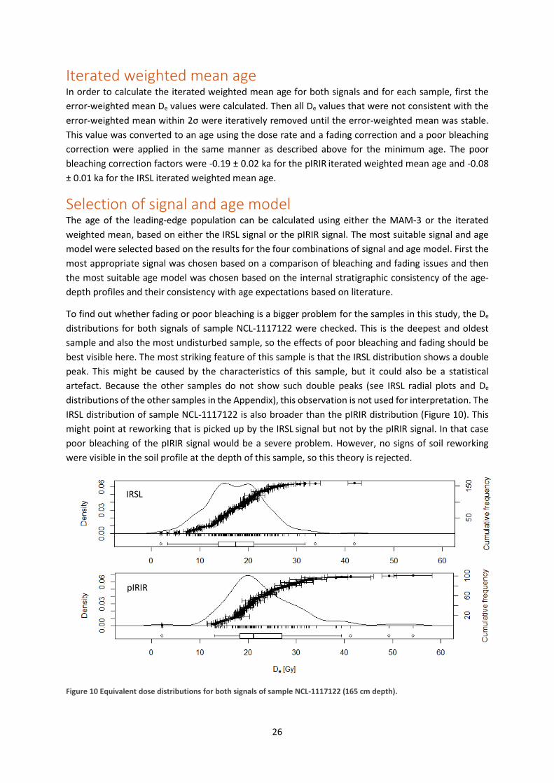
To find out whether fading or poor bleaching is a bigger problem for the samples in this study, the De
distributions for both signals of sample NCL-1117122 were checked. This is the deepest and oldest
sample and also the most undisturbed sample, so the effects of poor bleaching and fading should be
best visible here. The most striking feature of this sample is that the IRSL distribution shows a double
peak. This might be caused by the characteristics of this sample, but it could also be a statistical
artefact. Because the other samples do not show such double peaks (see IRSL radial plots and De
distributions of the other samples in the Appendix), this observation is not used for interpretation. The
IRSL distribution of sample NCL-1117122 is also broader than the pIRIR distribution (Figure 10). This
might point at reworking that is picked up by the IRSL signal but not by the pIRIR signal. In that case
poor bleaching of the pIRIR signal would be a severe problem. However, no signs of soil reworking
were visible in the soil profile at the depth of this sample, so this theory is rejected.
Figure 10 Equivalent dose distributions for both signals of sample NCL-1117122 (165 cm depth).
pIRIR
IRSL
27
Another explanation for the wide IRSL distribution could be that the fading rate of the IRSL signal is
less consistent over the total population of grains than for the pIRIR signal. This sample could contain
grains fading at different rates. In that case, the bulk fading rate is not representative for each
individual grain, because the fading rate of a grain depends on the rate at which a grain receives
radiation from its environment (Wallinga et al. 2007). If the IRSL signal indeed consists of different
grain populations fading at different rates, the pIRIR age is a better estimation of the burial age than
the IRSL age. Since evidence is present for fading problems but not for bleaching problems, the pIRIR
signal was considered most suitable for age calculation. If bleaching problems are small or absent for
a cover sand sample they are also expected to be small or absent for the samples in the reworking
zone, because reworking is assumed to be a better bleaching process than cover sand deposition. In
the reworking process grains are constantly and very intensively mixed and therefore they have more
bleaching possibilities than cover sand grains that are deposited in one single, relatively short event.
Another reason why the pIRIR signal is preferred over the IRSL signal is that the ages of the samples
taken in undisturbed cover sand parent material, which is known to be deposited at the end of the
Pleistocene, correspond well to this expected age. The fading corrected IRSL ages of this cover sand
sample were only 9.7 ka (weighted mean) and 9.8 ka (MAM), whereas the fading corrected ages of the
pIRIR signal were 11.2 ka (weighted mean) and 12.3 ka (MAM). The expected Pleistocene age of cover
sand (Zeeberg 1998) is around 11-12 ka, so the pIRIR weighted mean is more consistent with
chronostratigraphic evidence regarding the timing of cover sand activity.
After selection of the most appropriate signal, the most appropriate age model was selected. For some
samples, the conventional logged minimum age model could not be applied because of negative dose
measurements for individual grains. For these samples, the unlogged model had to be applied. This
resulted in a mixture of ages determined with the logged and unlogged age model. The ages older than
around 350 years that were calculated with the unlogged model were underestimated compared to
the ages calculated with the logged model, resulting in local age inversions. For sample NCL-1117133
the age was negative within the standard error (Appendix Table 7). Moreover, visual inspection of
radial plots and De distributions showed that the 2σ iterated weighted mean generally resulted in
equally good or better estimations of the minimum age peak than the minimum age model (see the
radial plots and De distributions in the Appendix). For these reasons, the iterated weighted mean age
was deemed more appropriate for age estimation.
The weighted mean age of sample NCL-1117123 (see pIRIR radial plot for this sample in the Appendix),
for which only a few measurements fall inside the 2σ bar, remains problematic. The weighted mean is
clearly an underestimation. However, the MAM seems to overestimate the age of the leading-edge De
population. The cause of these problems might be that the youngest grains in this sample do not form
a leading-edge peak in the distribution of this sample, but rather a plateau joining to the left side of
the main peak of undisturbed grains (see pIRIR De distribution for this sample in the Appendix).
28
Considering these arguments, the pIRIR iterated weighted mean age was chosen as best representative
of the leading-edge De population. The age-depth profile for this age seems to be divided in two parts
(Figure 11) with distinctly different age-depth gradients. In the upper part the age increases with depth
at a rate of 0.0087 ka/cm, whereas the age increases with 0.25 ka/cm in the lower part. The boundary
between the upper and lower part lies as a depth of approximately 120 cm. This division of the profile
in two parts could be caused by high accumulation rates and high soil reworking rates in the upper
part, related to plaggic agriculture. This hypothesis is supported by the fact that all layers in the upper
part have been ploughed (Figure 8 and Table 1). The reworking rates and accumulation rates are
discussed in the following sections.
Figure 11 Age-depth profile with gradients for the upper (<120 cm) and lower (>120 cm) part of the profile.
29
Soil reworking rates Effective soil reworking rates were determined for all samples according to the method proposed by
Reimann et al. (2017). They calculated reworking rates for a situation in which saturated feldspar grains
derived from weathered bedrock were present. These grains had never been exposed to daylight and
as a consequence they were never bleached, so their luminescence signal was infinitely large. In this
study no saturated grains are present, but the applied principle is the same. The method by Reimann
et al. (2017) can be generalised to other situations when the terms ‘unsaturated’ and ‘saturated’ are
replaced by the terms ‘reworked’ and ‘unreworked’ respectively. The non-saturation factor is then
replaced by a reworking intensity factor (RIF) that indicates the fraction of reworked grains in a sample.
This means that the RIF needs to be determined for both the reworked and unreworked samples,
because even in samples that are mostly undisturbed, a few percent of grains might be reworked by
bioturbation. In this study, the cover sand aged grains represent the unreworked fraction and all
younger grains form the reworked fraction. In determining the RIF, a distinction was made between
the upper (<120 cm) and lower (>120 cm) part of the soil profile. Soil reworking in the upper part of
the profile is the result of both biological and anthropogenic reworking, where the influence of the
latter is assumed to dominate because ploughing is a much more intensive mixing process than
bioturbation. The lower part of the profile has never been ploughed and mixing is exclusively the result
of bioturbation. For the lower part of the soil profile the RIF depends on the fraction of cover sand
aged grains present in the sample. The cover sand aged grains were separated from the reworked
grains using the finite mixture model by Galbraith (2005). The function calc_FiniteMixture in the R
package Luminescence was applied to the equivalent dose datasets trying 2 to 10 components. In all
three cases, the 2-component model resulted in the lowest BIC-value and was therefore the best fit to
the data (Schwarz 1978). The youngest component was assumed to represent the reworked grains and
the fraction of this component of the total sample was used as the RIF. The finite mixture model could
not be applied to the samples in the upper part of the profile, because of the presence of negative
equivalent dose measurements. The RIF in the upper part is assumed to be 1, because the historical
practice of stepwise application of a thin plaggic layer and ploughing can be assumed to fully bleach
every single-grain. This assumption appears to be a reasonable approximation, because the three RIF
values that could be calculated were 0.96 for the samples NCL-1117127 and NCL-1117131 and 0.89 for
sample NCL-1117132. For this latter sample application of the finite mixture model results in three
components, of which only the first one is considered to be cover sand. The dose of the middle
component is 3.55 ± 1.02 Gy and therefore much too young to be included in the cover sand fraction.
The presence of a few cover sand aged grains in this part of the profile is considered sample
contamination or upward movement of older grains. As expected, the soil reworking rates were indeed
higher in the upper part of the profile than in the lower part (Figure 12, Appendix Table 8). The
difference is one to two orders of magnitude. The rates in the upper part of the profile are showing
only a very small increase with depth, whereas the lower three samples are different from the upper
part and their reworking rates rapidly decrease with depth.
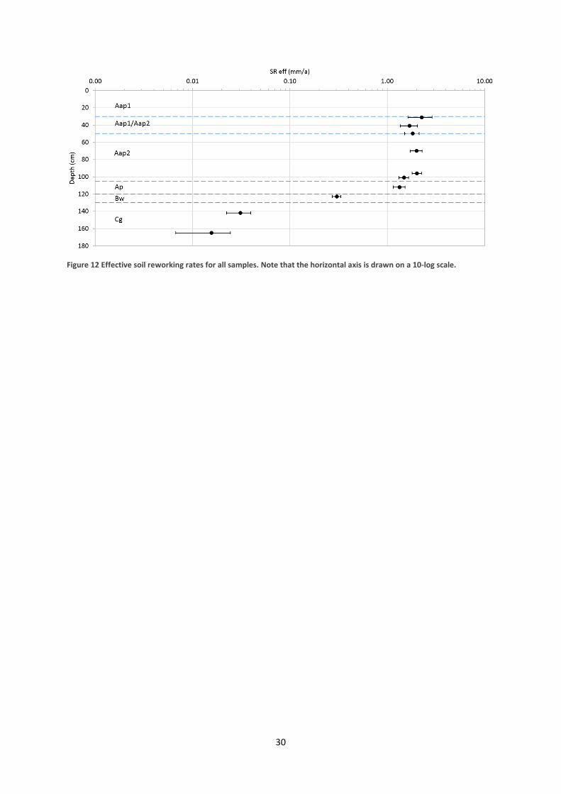
30
Figure 12 Effective soil reworking rates for all samples. Note that the horizontal axis is drawn on a 10-log scale.
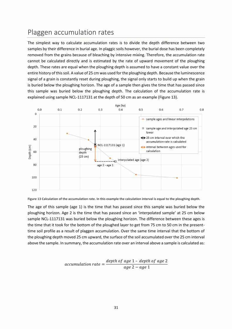
31
Plaggen accumulation rates The simplest way to calculate accumulation rates is to divide the depth difference between two
samples by their difference in burial age. In plaggic soils however, the burial dose has been completely
removed from the grains because of bleaching by intensive mixing. Therefore, the accumulation rate
cannot be calculated directly and is estimated by the rate of upward movement of the ploughing
depth. These rates are equal when the ploughing depth is assumed to have a constant value over the
entire history of this soil. A value of 25 cm was used for the ploughing depth. Because the luminescence
signal of a grain is constantly reset during ploughing, the signal only starts to build up when the grain
is buried below the ploughing horizon. The age of a sample then gives the time that has passed since
this sample was buried below the ploughing depth. The calculation of the accumulation rate is
explained using sample NCL-1117131 at the depth of 50 cm as an example (Figure 13).
Figure 13 Calculation of the accumulation rate. In this example the calculation interval is equal to the ploughing depth.
The age of this sample (age 1) is the time that has passed since this sample was buried below the
ploughing horizon. Age 2 is the time that has passed since an ‘interpolated sample’ at 25 cm below
sample NCL-1117131 was buried below the ploughing horizon. The difference between these ages is
the time that it took for the bottom of the ploughed layer to get from 75 cm to 50 cm in the present-
time soil profile as a result of plaggen accumulation. Over the same time interval that the bottom of
the ploughing depth moved 25 cm upward, the surface of the soil accumulated over the 25 cm interval
above the sample. In summary, the accumulation rate over an interval above a sample is calculated as:
𝑎𝑐𝑐𝑢𝑚𝑢𝑙𝑎𝑡𝑖𝑜𝑛 𝑟𝑎𝑡𝑒 =𝑑𝑒𝑝𝑡ℎ 𝑜𝑓 𝑎𝑔𝑒 1 – 𝑑𝑒𝑝𝑡ℎ 𝑜𝑓 𝑎𝑔𝑒 2
𝑎𝑔𝑒 2 − 𝑎𝑔𝑒 1
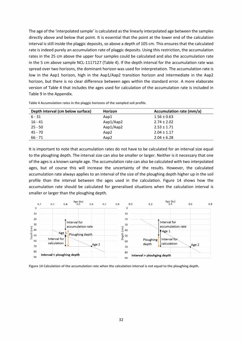
32
The age of the ‘interpolated sample’ is calculated as the linearly interpolated age between the samples
directly above and below that point. It is essential that the point at the lower end of the calculation
interval is still inside the plaggic deposits, so above a depth of 105 cm. This ensures that the calculated
rate is indeed purely an accumulation rate of plaggic deposits. Using this restriction, the accumulation
rates in the 25 cm above the upper four samples could be calculated and also the accumulation rate
in the 5 cm above sample NCL-1117127 (Table 4). If the depth interval for the accumulation rate was
spread over two horizons, the dominant horizon was used for interpretation. The accumulation rate is
low in the Aap1 horizon, high in the Aap1/Aap2 transition horizon and intermediate in the Aap2
horizon, but there is no clear difference between ages within the standard error. A more elaborate
version of Table 4 that includes the ages used for calculation of the accumulation rate is included in
Table 9 in the Appendix.
Table 4 Accumulation rates in the plaggic horizons of the sampled soil profile.
Depth interval (cm below surface) Horizon Accumulation rate (mm/a)
6 - 31 Aap1 1.56 ± 0.63 16 - 41 Aap1/Aap2 2.74 ± 2.02 25 - 50 Aap1/Aap2 2.53 ± 1.71 45 - 70 Aap2 2.04 ± 1.17 66 - 71 Aap2 2.04 ± 6.28
It is important to note that accumulation rates do not have to be calculated for an interval size equal
to the ploughing depth. The interval size can also be smaller or larger. Neither is it necessary that one
of the ages is a known sample age. The accumulation rate can also be calculated with two interpolated
ages, but of course this will increase the uncertainty of the results. However, the calculated
accumulation rate always applies to an interval of the size of the ploughing depth higher up in the soil
profile than the interval between the ages used in the calculation. Figure 14 shows how the
accumulation rate should be calculated for generalised situations when the calculation interval is
smaller or larger than the ploughing depth.
Figure 14 Calculation of the accumulation rate when the calculation interval is not equal to the ploughing depth.

33
Discussion and interpretation
Feldspar single-grain dating of plaggic soils in context This is the first application of feldspar single-grain luminescence dating to a plaggic anthrosol. This
method has shown to produce a chronologically consistent age-depth profile. Ages increase
systematically with depth and the expected end-Pleistocene age (Zeeberg 1998) of cover sand sample
NCL-1117122 is well reflected by the pIRIR iterated weighted mean age of 11.2 ± 0.9 ka determined
for that sample. The feldspar single-grain ages in the profile are in line with independent age estimates
determined by Smeenge (in preparation) using the well-established multiple grain quartz
luminescence dating method. An elaboration was made on the applications of the effective soil
reworking rate as developed by Reimann et al. (2017). Apart from situations in which saturated grains
from weathered bedrock are present in a reworked soil, the effective reworking rate can also be
calculated for purely sedimentary situations. This enabled quantification of the mixing processes in a
plaggic soil and it clearly showed the difference between natural and anthropogenic reworking. For
the first time historical accumulation rates in plaggic deposits have been calculated using luminescence
dating. These rates are useful for the reconstruction of former management practices and possibly
they are useful as well for improvement of modern agricultural techniques.
This shows the potential of single-grain feldspar luminescence dating for future dating applications. Its
results are very promising and although less feldspar than quartz is generally present in a sample, the
great advantage of feldspar is that much more grains emit a suitable luminescence signal. This makes
feldspar a very efficient mineral for luminescence dating and in particular for single-grain luminescence
dating. Because the quartz multiple grain ages by Smeenge (in preparation) were used to correct the
feldspar ages for poor bleaching, the feldspar ages determined here cannot be directly compared to
these quartz ages. To be able to compare the ages, a modern surface sample exposed to natural
daylight (modern analogue) should have been used to correct for poor bleaching. A real sample or an
extrapolated sample could have been used for this. The luminescence signal in such a sample is a good
estimate of the age inheritance due to incomplete signal resetting. In fact, such a correction would be
better even if ages were not to be compared because the poor bleaching correction using quartz ages
has an important shortcoming. The quartz ages used for correction have been linearly interpolated to
depth because the quartz samples and feldspar samples were taken at different depths. Since plaggen
application is a gradual process and since the soil is constantly reworked during this process, the age
increase with depth between two subsequent samples can indeed be considered linear. However, the
uncertainties of these quartz ages could not be interpolated. They were not included in the error-
weighted mean age, which has now only been based on the error on the feldspar age.
Start of plaggic agriculture To determine the moment at which plaggic agriculture started at the investigated location, the age
below the lowest plaggic horizon should be used. This age reflects the moment when the non-plaggic
soil was buried below the ploughing horizon as a result of the first plaggen addition. Sample NCL-
1117125 in the Ap horizon is the first sample below the Aap2 horizon. It has an age of 839 ± 113 a,
which indicates that plaggic agriculture started around 1178 ± 113 AD. This age is probably slightly
underestimated so that plaggic agriculture started to develop a little earlier. The reason for
underestimation is that the age is based on an error-weighted mean equivalent dose. The errors of the
De estimates of individual grains serve as a weighting factor with the more precise values getting a
34
higher weight. Since lower values generally have a lower absolute error, they have more effect on the
weighted mean than higher values. Galbraith and Roberts (2012) have observed the same for the
unlogged common age model, which is similar to the iterated weighted mean used here. When
standard errors of the De increase with increasing De value, the unlogged version of the common age
model may be biased towards the lower De values in a distribution, resulting in an age underestimation.
If the minimum age model would have been used instead of the weighted mean the same problem
would occur, because for the pIRIR signal of sample NCL-1117125 the unlogged common age model
had to be used. According to Arnold et al. (2009) the unlogged minimum age model gives accurate
burial doses and luminescence ages for samples younger than 350 a. For samples older than 350 a the
age is underestimated when using the unlogged minimum age model. Therefore, the pIRIR unlogged
MAM age of 627 ± 145 a for sample NCL-1117125 is an underestimation as well, and even more
severely than the weighted mean age.
Taking this underestimation into account, plaggic agriculture probably started a little earlier around
the beginning of the High Middle Ages (1000-1300 AD). In this subperiod of the Middle Ages the
European population increased and new areas of land were cultivated for agriculture (Bartlett 1994).
Knowledge on crops and agriculture expanded and better ploughing techniques were developed. The
start of plaggic agriculture as determined by feldspar single grain luminescence dating is consistent
with these historical events. The start of plaggic agriculture also coincides with the Medieval Warm
Period (950-1250 AD). The Medieval Warm Period was described by Lamb (1965) as a period in which
temperature changes of 1.2 to 1.4 °C and an annual rainfall increase of 10 % occurred in England. These
warmer and more humid conditions increased the number of crop types that could be grown. In
combination with improved agricultural techniques and increased food demand related to population
growth this led to a higher agricultural intensity and presumably also to the start of plaggic agriculture
at the sampled location.
Natural and anthropogenic soil reworking The rates in the upper part of the soil profile are the combined rates of natural and anthropogenic
reworking, whereas the rates in the lower part of the profile are purely natural. The soil reworking rates
increase suddenly at the boundary between those two parts. The reason for this sudden increase could be
that the upper part of the natural (non-plaggic) profile is not preserved. Soil reworking in this part was
probably of intermediate intensity, given the presence of a non-plaggic ploughing layer. For the upper part
of the profile, the effects of bioturbation and anthropogenic reworking cannot be separated. Bioturbation
is probably larger in the upper part than in the lower part, because the high organic matter content in
plaggic deposits leads to the presence of more soil fauna. Although bioturbation can be expected to be
larger in the upper part than in the lower part, the effect of ploughing on the reworking rate is expected
to dominate here. The natural effective reworking rates in the lower part of the profile are 0.02 ± 0.01
mm/a, 0.03 ± 0.01 mm/a and 0.30 ± 0.03 mm/a (Appendix Table 8). Comparable (apparent) rates of
0.1 to 0.5 mm/a and 0.03 to 0.2 mm/a were found by Stockmann et al. (2013). These rates were
determined in the upper 50 cm under a forest, so these rates are also based on exclusively natural
reworking. Reimann et al. (2017) found effective soil reworking rates up to 0.067 ± 0.010 mm/a for a
hillslope in Spain where mixing was only caused by natural processes. This similarity in reworking rates
with other natural reworking rates suggests that natural soil reworking at shallow depths happens at
a fairly constant rate, independent of the natural circumstances. The effective reworking rates in the
ploughed part of the profile are between 1.34 ± 0.18 mm/a and 2.26 ± 0.63 mm/a (Appendix Table 8).
As expected, these rates are much higher than the natural rates as a result of ploughing. This confirms
35
the initial hypothesis that anthropogenic reworking is dominant over natural reworking in the upper
part of the soil profile.
Some remarks should be made on the calculation of the reworking rates. The minimum overdispersion
σb was used as input for the finite mixture model. The overdispersion of the cover sand component
will indeed be close to σb, because the sample that was used to derive it (NCL-1117122) fully consists
of unmixed cover sand. However, the finite mixture model assumes that the overdispersion is the same
for all components, so in this case the overdispersion used for the reworked (mainly plaggic)
subpopulation will be equal to the overdispersion of the cover sand subpopulation. These two
components cannot be assumed to have equal overdispersion, because plaggen deposition occurs
slowly at a rate of about 1-2 mm/a while cover sand deposition is an instantaneous event. Therefore,
the overdispersion for perfectly bleached cover sand will be lower than for perfectly bleached plaggen
deposits and the value of σb will underestimate the overdispersion of the reworked fraction. In the
finite mixture model all fitted dose distributions depend on each other, because their proportions must
add up to one. Underestimation of the overdispersion of the reworking peak may therefore cause
overestimation of the number of components and erroneous mixing proportions (Galbraith and
Roberts 2012). The mean value and proportion (and as a consequence the RIF) of the cover sand peak
then partially depend on the other fitted distributions and this would lead to a wrong age estmation.
Another disadvantage of the finite mixture model is that the R function calc_FiniteMixture does not
consider the uncertainty of σb. This leads to extra uncertainty in the proportions and mean values of
all components.
Instead of using the finite mixture model, the cover sand grains could be separated from the reworked
grains with the maximum age model. This model calculates one single age that represents the
boundary between cover sand and reworked grains, namely the peak of the cover sand subpopulation.
The advantage is that this model calculates the mean value of the cover sand peak independently of
the other peaks. However, the uncertainty of σb is not taken into account by the R function
calc_MaxDose either and, more importantly, the lower half of the cover sand peak would be
incorporated in the proportion of reworked grains. The finite mixture model does not use a rigid age
boundary between the reworked grains and cover sand grains. Whereas the maximum age model does
not consider the uncertainties of the boundary age and the individual De values, the finite mixture
model does consider all these uncertainties. This leads to a much more reliable estimate of the
proportions of cover sand grains and reworked grains in a sample, so the finite mixture model was
preferred over the maximum age model.
Historical accumulation of plaggen Based on the accumulation rates obtained for this location, historical plaggen accumulation seems to
be divided in three phases. In the first phase the Aap2 horizon was formed at a seemingly constant
rate of 2.04 mm/a (two values of 2.04 ± 1.17 mm/a and 2.04 ± 6.28 mm/a were measured). The second
phase is characterised by more rapid accumulation rates in the Aap1/Aap2 horizon of 2.53 ± 1.71 mm/a
and 2.74 ± 2.02 mm/a. Above this transition horizon the accumulation rate appears to be lower with a
value of 1.56 ± 0.63 mm/a. This marks the third accumulation phase related to the formation of the
Aap1 horizon. Within one standard error the accumulation rates do not differ a lot between the three
phases, so the division in three phases should be considered with some caution. As discussed earlier,
the first phase of plaggen accumulation starts at the beginning of the High Middle Ages. The European
population was already growing, but not as fast as in later stages. Probably the development of
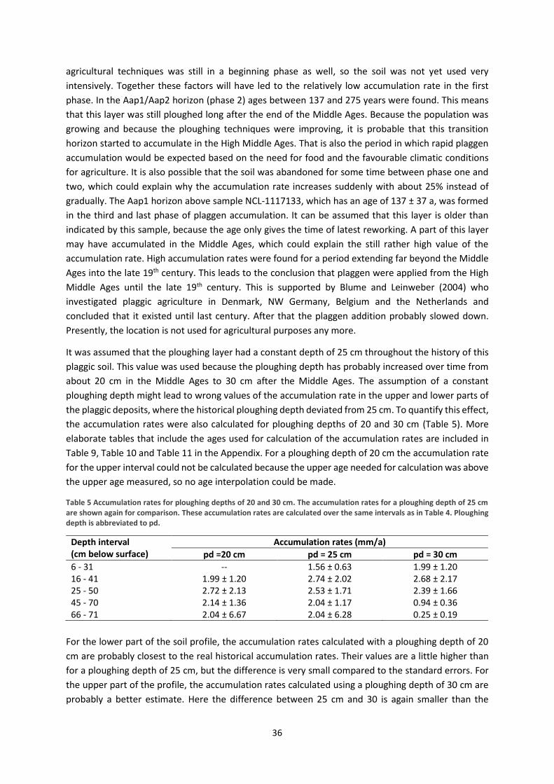
36
agricultural techniques was still in a beginning phase as well, so the soil was not yet used very
intensively. Together these factors will have led to the relatively low accumulation rate in the first
phase. In the Aap1/Aap2 horizon (phase 2) ages between 137 and 275 years were found. This means
that this layer was still ploughed long after the end of the Middle Ages. Because the population was
growing and because the ploughing techniques were improving, it is probable that this transition
horizon started to accumulate in the High Middle Ages. That is also the period in which rapid plaggen
accumulation would be expected based on the need for food and the favourable climatic conditions
for agriculture. It is also possible that the soil was abandoned for some time between phase one and
two, which could explain why the accumulation rate increases suddenly with about 25% instead of
gradually. The Aap1 horizon above sample NCL-1117133, which has an age of 137 ± 37 a, was formed
in the third and last phase of plaggen accumulation. It can be assumed that this layer is older than
indicated by this sample, because the age only gives the time of latest reworking. A part of this layer
may have accumulated in the Middle Ages, which could explain the still rather high value of the
accumulation rate. High accumulation rates were found for a period extending far beyond the Middle
Ages into the late 19th century. This leads to the conclusion that plaggen were applied from the High
Middle Ages until the late 19th century. This is supported by Blume and Leinweber (2004) who
investigated plaggic agriculture in Denmark, NW Germany, Belgium and the Netherlands and
concluded that it existed until last century. After that the plaggen addition probably slowed down.
Presently, the location is not used for agricultural purposes any more.
It was assumed that the ploughing layer had a constant depth of 25 cm throughout the history of this
plaggic soil. This value was used because the ploughing depth has probably increased over time from
about 20 cm in the Middle Ages to 30 cm after the Middle Ages. The assumption of a constant
ploughing depth might lead to wrong values of the accumulation rate in the upper and lower parts of
the plaggic deposits, where the historical ploughing depth deviated from 25 cm. To quantify this effect,
the accumulation rates were also calculated for ploughing depths of 20 and 30 cm (Table 5). More
elaborate tables that include the ages used for calculation of the accumulation rates are included in
Table 9, Table 10 and Table 11 in the Appendix. For a ploughing depth of 20 cm the accumulation rate
for the upper interval could not be calculated because the upper age needed for calculation was above
the upper age measured, so no age interpolation could be made.
Table 5 Accumulation rates for ploughing depths of 20 and 30 cm. The accumulation rates for a ploughing depth of 25 cm are shown again for comparison. These accumulation rates are calculated over the same intervals as in Table 4. Ploughing depth is abbreviated to pd.
Depth interval (cm below surface)
Accumulation rates (mm/a)
pd =20 cm pd = 25 cm pd = 30 cm
6 - 31 -- 1.56 ± 0.63 1.99 ± 1.20 16 - 41 1.99 ± 1.20 2.74 ± 2.02 2.68 ± 2.17 25 - 50 2.72 ± 2.13 2.53 ± 1.71 2.39 ± 1.66 45 - 70 2.14 ± 1.36 2.04 ± 1.17 0.94 ± 0.36 66 - 71 2.04 ± 6.67 2.04 ± 6.28 0.25 ± 0.19
For the lower part of the soil profile, the accumulation rates calculated with a ploughing depth of 20
cm are probably closest to the real historical accumulation rates. Their values are a little higher than
for a ploughing depth of 25 cm, but the difference is very small compared to the standard errors. For
the upper part of the profile, the accumulation rates calculated using a ploughing depth of 30 cm are
probably a better estimate. Here the difference between 25 cm and 30 is again smaller than the
37
standard errors, so the assumption of a ploughing depth of 25 cm seems to be appropriate for the
whole profile. If instead the ploughing depth was varied from 20 cm to 30 cm, the general
interpretation of the three phases of accumulation would still be valid, though the differences between
the phases would be smaller. A striking effect occurs when a ploughing depth of 30 cm is applied for
the lower part of the soil profile. The calculated accumulation rates are very low and precise. The low
value is the result of the large age-depth gradient between the points that were used to derive the
accumulation rate (Table 11). The accumulation rates are also very precise as a consequence of the
same large age-depth gradient and of the low values of the accumulation rates themselves, because
both factors are included in the error calculation.
38
Conclusions Single-grain feldspar luminescence dating was used to derive ages at several depths inside a plaggic
anthrosol. Analysis of the soil profile showed that at this location plaggic agriculture first appeared
around the beginning of the High Middle Ages (1000-1300 AD). At this time the European population
started to grow and agricultural techniques improved. The appearance of plaggic agriculture can also
be linked to the Medieval Warm Period (950-1250 AD), in which elevated temperature and humidity
increased agricultural possibilities. Plaggic agriculture thrived during this period, as can be derived
from the rapid accumulation rates. After the Middle Ages, plaggen accumulation slowed down and the
soil at the sampling location was not ploughed any more. Effective soil reworking rates at several
depths in the soil profile revealed the impact of human activity on soil mixing. The difference between
natural soil reworking and reworking by ploughing has been quantified for the first time using feldspar
single-grain luminescence dating. A substantial difference in reworking rate of one to two orders of
magnitude between both mixing processes was found. The feldspar single-grain ages are all consistent
with independent quartz multiple grain OSL age estimates derived from different samples taken at the
same location. An important advantage of dating single feldspar grains over dating single quartz grains
is that a much larger percentage of the feldspar grains emits a suitable luminescence signal. This
property combined with the consistency of the ages with independent age estimates from a well-
established method and with the dates of historical events shows the potential of this new method for
future applications.

39
Acknowledgements I would like to thank Harm Smeenge for letting me use the yet unpublished quartz luminescence ages
of his PhD research. I also thank Mr. Borgerink for allowing me to take samples on his field, Erwin
Steijsiger for his help during field work, Erna Voskuilen for teaching me all necessary lab skills, Alice
Versendaal for her help with R and Matlab and of course both of my supervisors, Tony Reimann for his
enthusiasm and the helpful discussions and Jakob Wallinga for his critical view on decisive moments
throughout the process of this thesis.
40
References AHN (2012). Interpolated AHN2 0.5 meter maaiveld raster, kaartblad 29cn2, Actueel Hoogtebestand Nederland: downloaded from pdok.nl on 14 July 2017.
Arnold, L. J., R. Bailey and G. Tucker (2007). "Statistical treatment of fluvial dose distributions from southern Colorado arroyo deposits." Quaternary Geochronology 2(1): 162-167.
Arnold, L. J., R. G. Roberts, R. F. Galbraith and S. DeLong (2009). "A revised burial dose estimation procedure for optical dating of young and modern-age sediments." Quaternary Geochronology 4(4): 306-325.
Bartlett, R. (1994). The making of Europe: conquest, colonization and cultural change 950-1350, Penguin UK.
Bateman, M. D., C. D. Frederick, M. K. Jaiswal and A. K. Singhvi (2003). "Investigations into the potential effects of pedoturbation on luminescence dating." Quaternary Science Reviews 22(10): 1169-1176.
Behre, K.-E. (2000). "Fruhe Ackersysteme, Dungemethoden und die Entstehung der nordwestdeutschen Heiden." Archaologisches Korrespondenzblatt 30(1): 135-151.
Blume, H. P. and P. Leinweber (2004). "Plaggen soils: landscape history, properties, and classification." Journal of Plant Nutrition and Soil Science 167(3): 319-327.
Bokhorst, M., G. Duller and J. Van Mourik (2005). "Optical dating of a Fimic Anthrosol in the southern Netherlands." Journal of Archaeological Science 32(4): 547-553.
Castel, I., E. Koster and R. Slotboom (1989). "Morphogenetic aspects and age of Late Holocene eolian drift sands in Northwest Europe." Zeitschrift fur Geomorphologie 33(1): 1-26.
Cordell, D., J.-O. Drangert and S. White (2009). "The story of phosphorus: global food security and food for thought." Global environmental change 19(2): 292-305.
Cunningham, A. C. and J. Wallinga (2012). "Realizing the potential of fluvial archives using robust OSL chronologies." Quaternary Geochronology 12: 98-106.
Demuro, M., L. J. Arnold, D. G. Froese and R. G. Roberts (2013). "OSL dating of loess deposits bracketing Sheep Creek tephra beds, northwest Canada: dim and problematic single-grain OSL characteristics and their effect on multi-grain age estimates." Quaternary Geochronology 15: 67-87.
Dudal, R. and P. Driessen (1991). The major soils of the world: Lecture notes on their geography, formation, properties and use.
41
Duller, G. (2006). "Single grain optical dating of glacigenic deposits." Quaternary Geochronology 1(4): 296-304.
Duller, G. (2015). "The Analyst software package for luminescence data: overview and recent improvements." Ancient TL 33(1): 35-42.
Duller, G. A. (2008). "Single‐grain optical dating of Quaternary sediments: why aliquot size matters in luminescence dating." Boreas 37(4): 589-612.
Efron, B. and R. Tibshirani (1993). An Introduction to the Bootstrap New York, Chapman and Hall.
Fastabend, H. and F. von Raupach (1962). "Ergebnisse der C14-Untersuchungen an einigen Plaggenböden des Emslandes." Geol. Jb. 79: 863-866.
Freibauer, A., M. D. Rounsevell, P. Smith and J. Verhagen (2004). "Carbon sequestration in the agricultural soils of Europe." Geoderma 122(1): 1-23.
Galbraith, R. F. (2005). Statistics for fission track analysis, CRC Press.
Galbraith, R. F. and R. G. Roberts (2012). "Statistical aspects of equivalent dose and error calculation and display in OSL dating: an overview and some recommendations." Quaternary Geochronology 11: 1-27.
Galbraith, R. F., R. G. Roberts, G. M. Laslett, H. Yoshida and J. M. Olley (1999). "Optical dating of single and multiple grains of quartz from Jinmium rock shelter, northern Australia: Part I, experimental design and statistical models." Archaeometry 41(2): 339-364.
Giani, L., L. Makowsky and K. Mueller (2014). "Plaggic Anthrosol: Soil of the Year 2013 in Germany: An overview on its formation, distribution, classification, soil function and threats." Journal of Plant Nutrition and Soil Science 177(3): 320-329.
Gliganic, L., J.-H. May and T. J. Cohen (2015). "All mixed up: Using single-grain equivalent dose distributions to identify phases of pedogenic mixing on a dryland alluvial fan." Quaternary International 362: 23-33.
Gliganic, L. A., T. J. Cohen, M. Slack and J. K. Feathers (2016). "Sediment mixing in aeolian sandsheets identified and quantified using single-grain optically stimulated luminescence." Quaternary Geochronology 32: 53-66.
Godfrey-Smith, D. I., D. J. Huntley and W.-H. Chen (1988). "Optical dating studies of quartz and feldspar sediment extracts." Quaternary Science Reviews 7(3-4): 373-380.
42
Heimsath, A. M., J. Chappell, N. A. Spooner and D. G. Questiaux (2002). "Creeping soil." Geology 30(2): 111-114.
Heineman, B. (1973). "Bodenkundliche Untersuchungen an einem Megalithgrab unter Plaggenesch in Osnabrück-Nahne." Nachr. Nieders. Urgesch. 42: 211-219.
Hülle, D., A. Hilgers, P. Kühn and U. Radtke (2009). "The potential of optically stimulated luminescence for dating periglacial slope deposits—A case study from the Taunus area, Germany." Geomorphology 109(1): 66-78.
Huntley, D. J. and M. Lamothe (2001). "Ubiquity of anomalous fading in K-feldspars and the measurement and correction for it in optical dating." Canadian Journal of Earth Sciences 38(7): 1093-1106.
Jain, M. and C. Ankjærgaard (2011). "Towards a non-fading signal in feldspar: insight into charge transport and tunnelling from time-resolved optically stimulated luminescence." Radiation Measurements 46(3): 292-309.
Jain, M., J.-P. Buylaert, K. J. Thomsen and A. S. Murray (2015). "Further investigations on ‘non-fading’in K-Feldspar." Quaternary International 362: 3-7.
Kars, R. H., T. Reimann, C. Ankjærgaard and J. Wallinga (2014). "Bleaching of the post‐IR IRSL signal: new insights for feldspar luminescence dating." Boreas 43(4): 780-791.
Kristensen, J. A., K. J. Thomsen, A. S. Murray, J.-P. Buylaert, M. Jain and H. Breuning-Madsen (2015). "Quantification of termite bioturbation in a savannah ecosystem: application of OSL dating." Quaternary Geochronology 30: 334-341.
Lamb, H. H. (1965). "The early medieval warm epoch and its sequel." Palaeogeography, Palaeoclimatology, Palaeoecology 1: 13-37.
Lukas, S., J. Q. Spencer, R. A. Robinson and D. I. Benn (2007). "Problems associated with luminescence dating of Late Quaternary glacial sediments in the NW Scottish Highlands." Quaternary Geochronology 2(1): 243-248.
Lungershausen, U., A. Larsen, H.-R. Bork and R. Duttmann (2017). "Anthropogenic influence on rates of aeolian dune activity within the northern European Sand Belt and socio-economic feedbacks over the last 2500 years." The Holocene: 0959683617715693.
Merante, P., C. Dibari, R. Ferrise, B. Sánchez, A. Iglesias, J. P. Lesschen, P. Kuikman, J. Yeluripati, P. Smith and M. Bindi (2017). "Adopting soil organic carbon management practices in soils of varying quality: Implications and perspectives in Europe." Soil and Tillage Research 165: 95-106.
43
Mucher, H., R. Slotboom and W. Ten Veen (1989). "Een enkeerdgrond palynologisch ontsloten; toepssing van de palynologie bij de toetsieng van en de aanvulling op archivalische data." Geografisch Tijdschrift 23: 109-118.
Murray, A. and R. Roberts (1998). "Measurement of the equivalent dose in quartz using a regenerative-dose single-aliquot protocol." Radiation Measurements 29(5): 503-515.
Murray, A., K. J. Thomsen, N. Masuda, J.-P. Buylaert and M. Jain (2012). "Identifying well-bleached quartz using the different bleaching rates of quartz and feldspar luminescence signals." Radiation Measurements 47(9): 688-695.
Niemeier, G. and W. Taschenmacher (1939). "Plaggenböden. Beiträge zu ihrer genetik und typologie." Westfalische Forschungen 2: 29-64.
Olley, J. M., R. G. Roberts and A. S. Murray (1997). "Disequilibria in the uranium decay series in sedimentary deposits at Allen's Cave, Nullarbor Plain, Australia: implications for dose rate determinations." Radiation Measurements 27(2): 433-443.
Pape, J. (1970). "Plaggen soils in the Netherlands." Geoderma 4(3): 229-255.
Pietsch, T. J., J. M. Olley and G. C. Nanson (2008). "Fluvial transport as a natural luminescence sensitiser of quartz." Quaternary Geochronology 3(4): 365-376.
Prescott, J. R. and J. T. Hutton (1994). "Cosmic ray contributions to dose rates for luminescence and ESR dating: large depths and long-term time variations." Radiation Measurements 23(2-3): 497-500.
Preusser, F., D. Degering, M. Fuchs, A. Hilgers, A. Kadereit, N. Klasen, M. Krbetschek, D. Richter and J. Q. Spencer (2008). "Luminescence dating: basics, methods and applications." Quaternary Science Journal 57(1-2): 95-149.
Reimann, T., A. Román-Sánchez, T. Vanwalleghem and J. Wallinga (2017). "Getting a grip on soil reworking-Single-grain feldspar luminescence as a novel tool to quantify soil reworking rates." Quaternary Geochronology.
Reimann, T., K. J. Thomsen, M. Jain, A. S. Murray and M. Frechen (2012). "Single-grain dating of young sediments using the pIRIR signal from feldspar." Quaternary Geochronology 11: 28-41.
Reimann, T., S. Tsukamoto, M. Naumann and M. Frechen (2011). "The potential of using K-rich feldspars for optical dating of young coastal sediments–a test case from Darss-Zingst peninsula (southern Baltic Sea coast)." Quaternary Geochronology 6(2): 207-222.
Sandvik, B. (2009). Shapefile of the Netherlands: downloaded from thematicmapping.org on 14 July 2017.
44
Sawakuchi, A. O., C. Guedes, R. DeWitt, P. C. F. Giannini, M. Blair, D. Nascimento and F. Faleiros (2012). "Quartz OSL sensitivity as a proxy for storm activity on the southern Brazilian coast during the Late Holocene." Quaternary Geochronology 13: 92-102.
Schwarz, G. (1978). "Estimating the dimensions of a model." The annals of statistics 6(2): 461-464.
Smedley, R., G. Duller, N. Pearce and H. Roberts (2012). "Determining the K-content of single-grains of feldspar for luminescence dating." Radiation Measurements 47(9): 790-796.
Smeenge, H. (in preparation). PhD Thesis.
Spek, T. (2004). Het Drentse esdorpenlandschap; een historisch-geografische studie.
Spooner, N. A. (1994). "The anomalous fading of infrared-stimulated luminescence from feldspars." Radiation Measurements 23(2-3): 625-632.
Stockmann, U., B. Minasny, T. Pietsch and A. McBratney (2013). "Quantifying processes of pedogenesis using optically stimulated luminescence." European Journal of Soil Science 64(1): 145-160.
Thomsen, K. J., A. S. Murray, M. Jain and L. Bøtter-Jensen (2008). "Laboratory fading rates of various luminescence signals from feldspar-rich sediment extracts." Radiation Measurements 43(9-10): 1474-1486.
Van Mourik, J., A. Seijmonsbergen, R. Slotboom and J. Wallinga (2012). "Impact of human land use on soils and landforms in cultural landscapes on aeolian sandy substrates (Maashorst, SE-Netherlands)." Quaternary International 265: 74-89.
Van Mourik, J., R. Slotboom and J. Wallinga (2011). "Chronology of plaggic deposits; palynology, radiocarbon and optically stimulated luminescence dating of the Posteles (NE-Netherlands)." Catena 84(1): 54-60.
Van Mourik, J., P. Wartenbergh, W. Mook and H. Streurman (1995). "Radiocarbon dating of paleosols in aeolian sands." Mededelingen Rijks Geologische Dienst 52.
Wallinga, J., A. J. Bos, P. Dorenbos, A. S. Murray and J. Schokker (2007). "A test case for anomalous fading correction in IRSL dating." Quaternary Geochronology 2(1): 216-221.
Wilkinson, M. T., P. J. Richards and G. S. Humphreys (2009). "Breaking ground: pedological, geological, and ecological implications of soil bioturbation." Earth-Science Reviews 97(1): 257-272.
Zeeberg, J. (1998). "The European sand belt in eastern Europe and comparison of Late Glacial dune orientation with GCM simulation results." Boreas 27(2): 127-139.
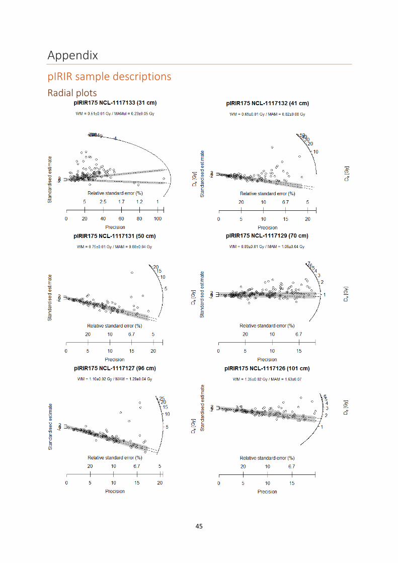
45
Appendix
pIRIR sample descriptions
Radial plots
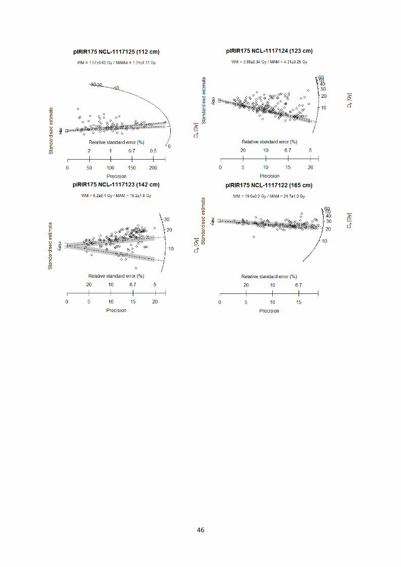
46
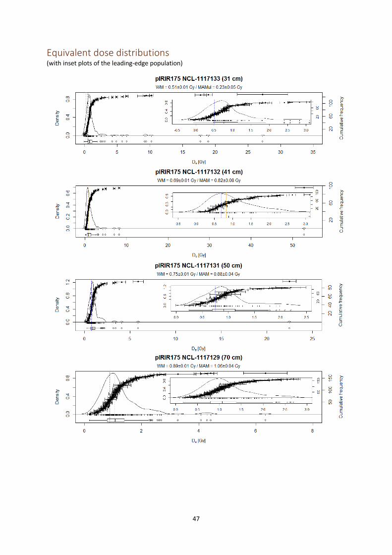
47
Equivalent dose distributions (with inset plots of the leading-edge population)
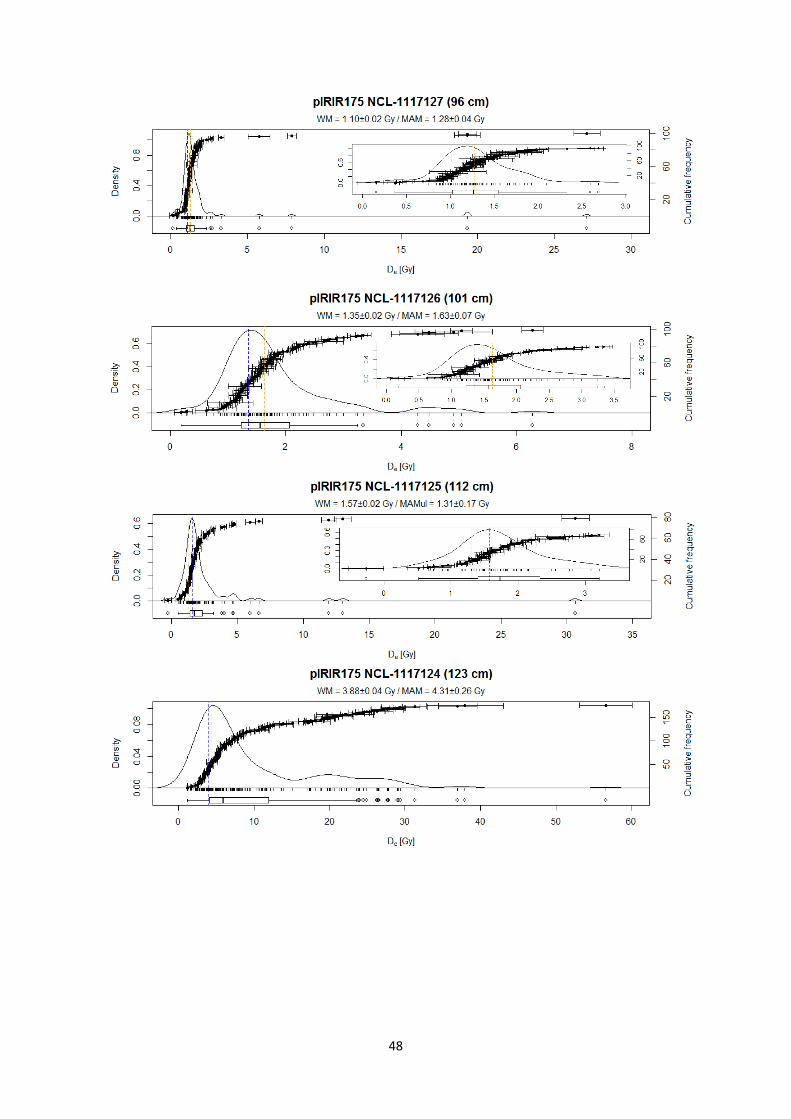
48
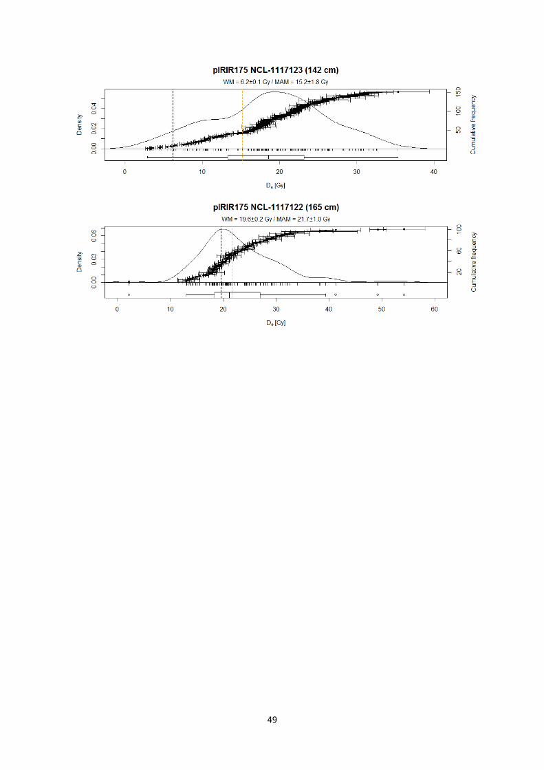
49
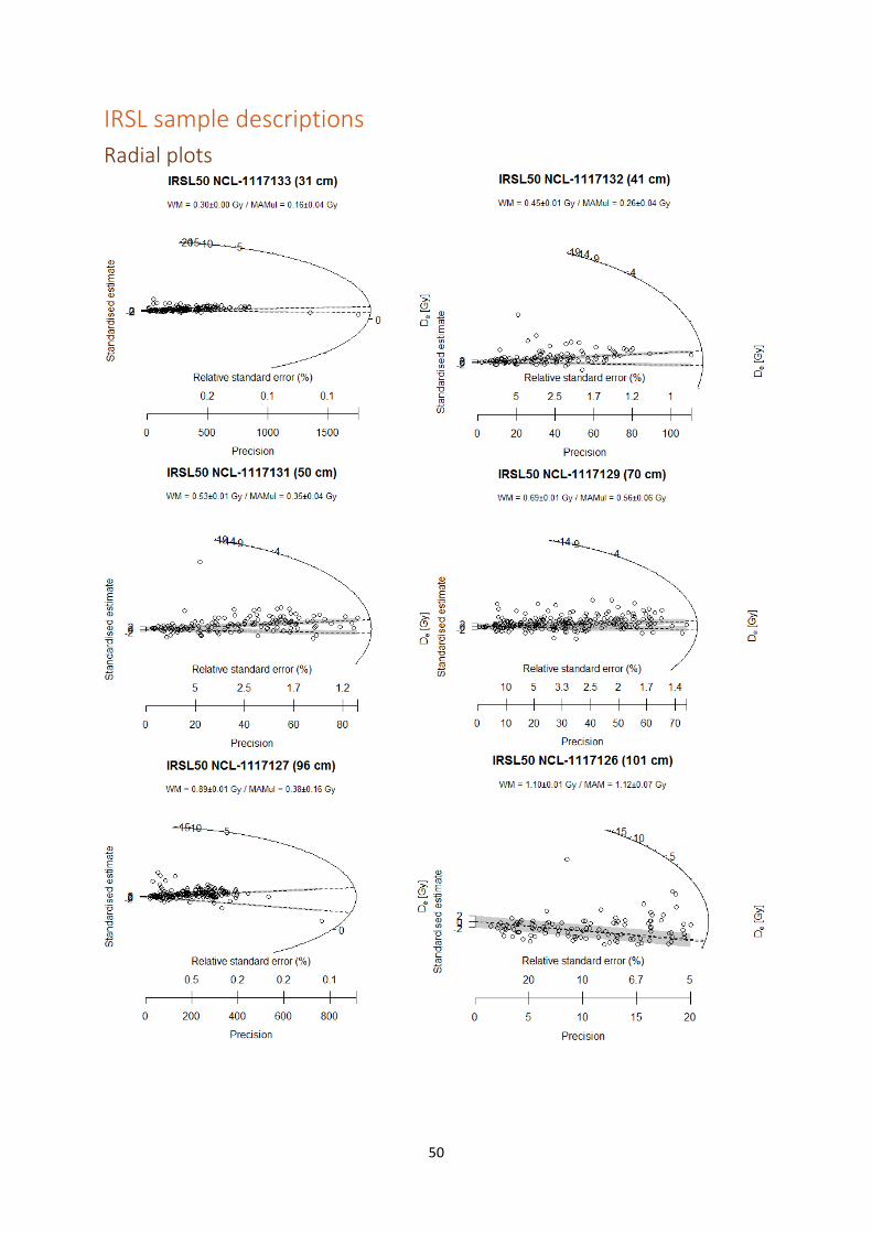
50
IRSL sample descriptions
Radial plots
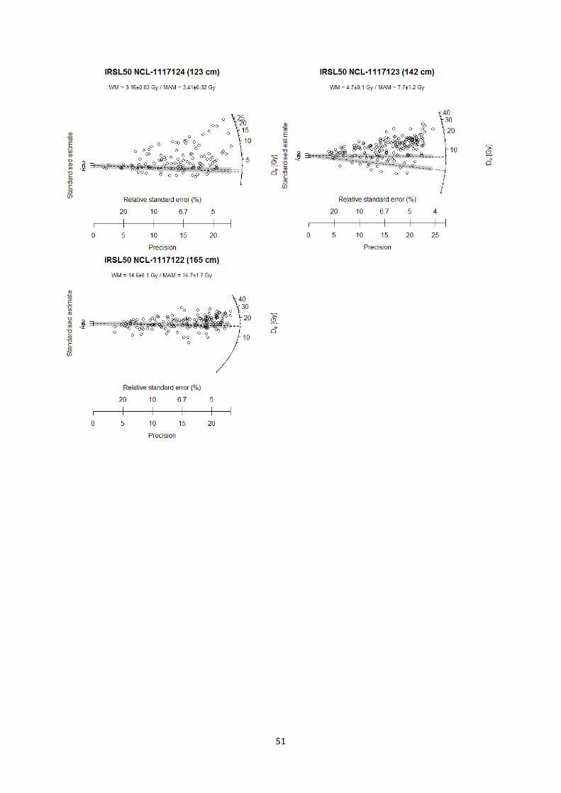
51
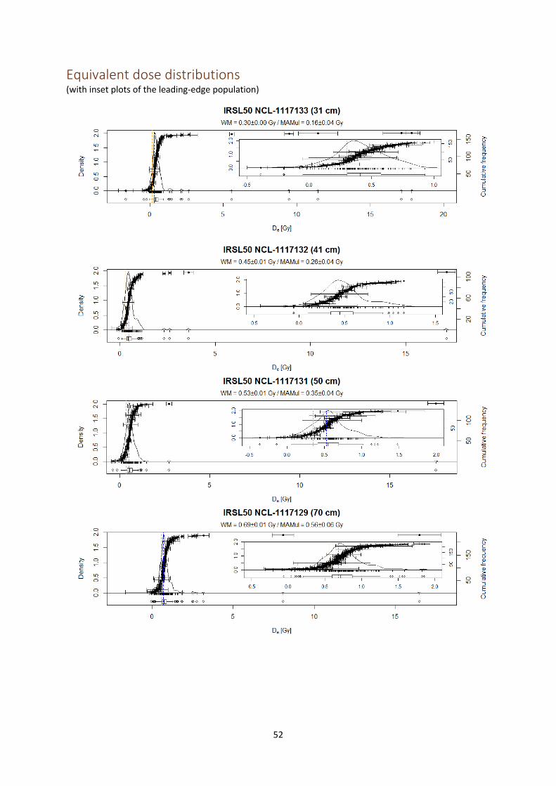
52
Equivalent dose distributions (with inset plots of the leading-edge population)
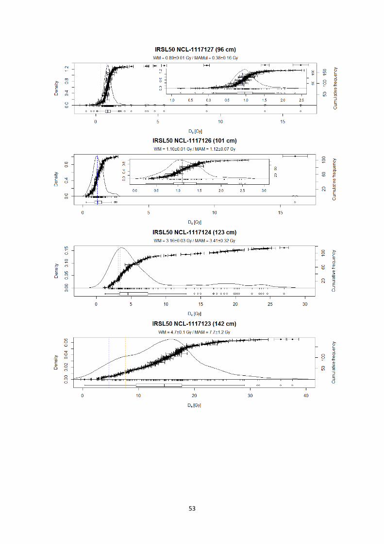
53
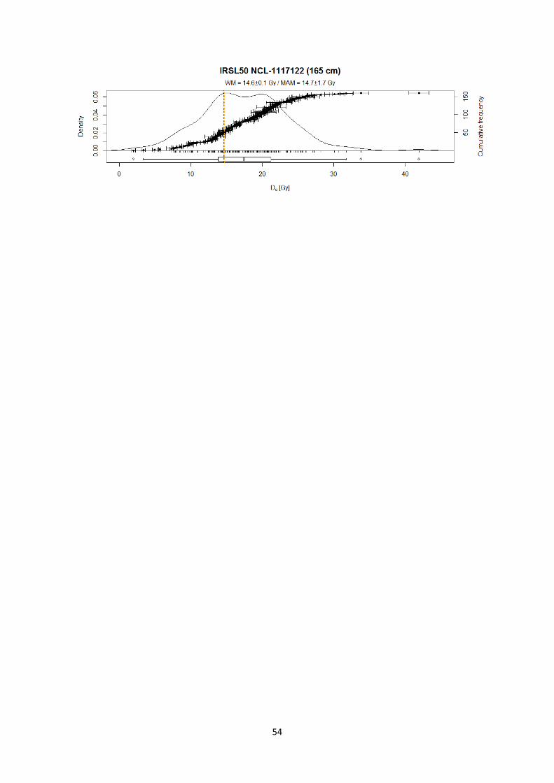
54

55
Result tables
Overdispersion Table 6 Overdispersion per sample for both signals
Sample Depth (cm) pIRIR overdispersion (%) IRSL overdispersion (%)
NCL-1117133 31 32.9 ± 7.7 36.9 ± 3.9 NCL-1117132 41 46.2 ± 3.7 53.7 ± 3.6 NCL-1117131 50 74.4 ± 3.3 69.3 ± 4.6 NCL-1117129 70 39.6 ± 4.1 39.7 ± 8.5 NCL-1117127 96 39.0 ± 4.3 53.0 ± 9.7 NCL-1117126 101 58.8 ± 12.8 28.8 ± 2.7 NCL-1117125 112 44.7 ± 3.6 -- NCL-1117124 123 54.0 ± 10.0 34.4 ± 3.5 NCL-1117123 142 76.9 ± 12.5 42.9 ± 4.9 NCL-1117122 165 59.8 ± 6.2 53.2 ± 4.9
Ages Table 7 Weighted mean and MAM-3 ages for the pIRIR and IRSL signal. Ages calculated with the unlogged MAM-3 are marked with a *.
Sample Depth (cm) pIRIR weighted mean age (ka)
pIRIR MAM-3 age (ka)
IRSL weighted mean age (ka)
IRSL MAM-3 age (ka)
NCL-1117133 31 0.14 ± 0.04 -0.08 ± 0.07 * 0.12 ± 0.03 0.14 ± 0.03 * NCL-1117132 41 0.24 ± 0.05 0.29 ± 0.07 0.23 ± 0.03 0.21 ± 0.03 * NCL-1117131 50 0.27 ± 0.05 0.31 ± 0.06 0.27 ± 0.04 0.26 ± 0.04 * NCL-1117129 70 0.35 ± 0.05 0.40 ± 0.07 0.37 ± 0.04 0.40 ± 0.05 * NCL-1117127 96 0.48 ± 0.05 0.54 ± 0.08 0.51 ± 0.06 0.28 ± 0.12 * NCL-1117126 101 0.68 ± 0.08 0.82 ± 0.11 0.70 ± 0.08 0.83 ± 0.10 NCL-1117125 112 0.84 ± 0.11 0.63 ± 0.14 * -- -- NCL-1117124 123 2.3 ± 0.2 2.5 ± 0.3 2.2 ± 0.2 2.5 ± 0.3 NCL-1117123 142 3.6 ± 0.4 9.0 ± 1.5 3.1 ± 0.3 5.4 ± 1.0 NCL-1117122 165 11.2 ± 0.9 12.3 ± 1.1 9.7 ± 0.8 9.8 ± 1.5
Soil reworking rates Table 8 Soil reworking rates based on the pIRIR weighted mean age.
Sample Depth (cm) Soil reworking rate (mm/a)
NCL-1117133 31 2.26 ± 0.63 NCL-1117132 41 1.69 ± 0.34 NCL-1117131 50 1.82 ± 0.31 NCL-1117129 70 2.01 ± 0.27 NCL-1117127 96 2.01 ± 0.22 NCL-1117126 101 1.49 ± 0.17 NCL-1117125 112 1.34 ± 0.18 NCL-1117124 123 0.30 ± 0.03 NCL-1117123 142 0.03 ± 0.01 NCL-1117122 165 0.02 ± 0.01
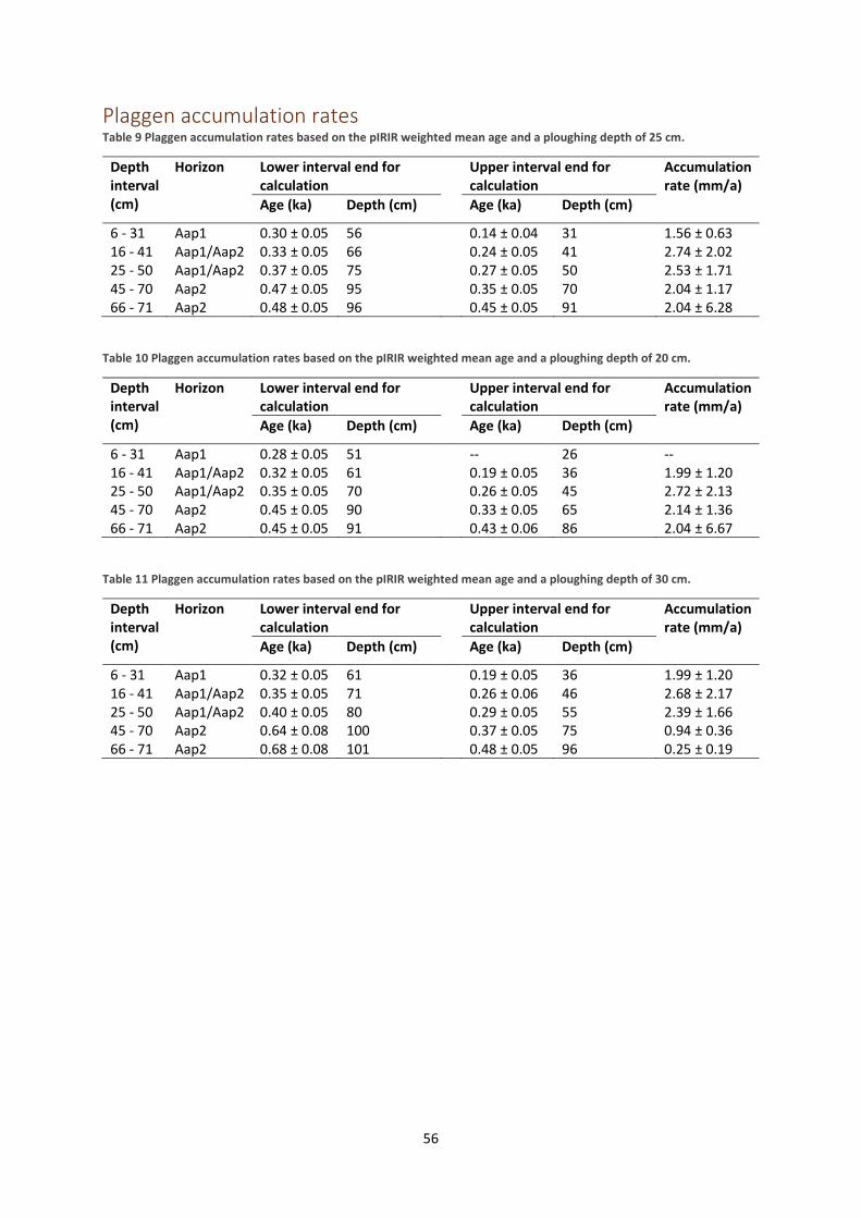
56
Plaggen accumulation rates Table 9 Plaggen accumulation rates based on the pIRIR weighted mean age and a ploughing depth of 25 cm.
Depth interval (cm)
Horizon Lower interval end for calculation
Upper interval end for calculation
Accumulation rate (mm/a)
Age (ka) Depth (cm) Age (ka) Depth (cm)
6 - 31 Aap1 0.30 ± 0.05 56 0.14 ± 0.04 31 1.56 ± 0.63 16 - 41 Aap1/Aap2 0.33 ± 0.05 66 0.24 ± 0.05 41 2.74 ± 2.02 25 - 50 Aap1/Aap2 0.37 ± 0.05 75 0.27 ± 0.05 50 2.53 ± 1.71 45 - 70 Aap2 0.47 ± 0.05 95 0.35 ± 0.05 70 2.04 ± 1.17 66 - 71 Aap2 0.48 ± 0.05 96 0.45 ± 0.05 91 2.04 ± 6.28
Table 10 Plaggen accumulation rates based on the pIRIR weighted mean age and a ploughing depth of 20 cm.
Depth interval (cm)
Horizon Lower interval end for calculation
Upper interval end for calculation
Accumulation rate (mm/a)
Age (ka) Depth (cm) Age (ka) Depth (cm)
6 - 31 Aap1 0.28 ± 0.05 51 -- 26 -- 16 - 41 Aap1/Aap2 0.32 ± 0.05 61 0.19 ± 0.05 36 1.99 ± 1.20 25 - 50 Aap1/Aap2 0.35 ± 0.05 70 0.26 ± 0.05 45 2.72 ± 2.13 45 - 70 Aap2 0.45 ± 0.05 90 0.33 ± 0.05 65 2.14 ± 1.36 66 - 71 Aap2 0.45 ± 0.05 91 0.43 ± 0.06 86 2.04 ± 6.67
Table 11 Plaggen accumulation rates based on the pIRIR weighted mean age and a ploughing depth of 30 cm.
Depth interval (cm)
Horizon Lower interval end for calculation
Upper interval end for calculation
Accumulation rate (mm/a)
Age (ka) Depth (cm) Age (ka) Depth (cm)
6 - 31 Aap1 0.32 ± 0.05 61 0.19 ± 0.05 36 1.99 ± 1.20 16 - 41 Aap1/Aap2 0.35 ± 0.05 71 0.26 ± 0.06 46 2.68 ± 2.17 25 - 50 Aap1/Aap2 0.40 ± 0.05 80 0.29 ± 0.05 55 2.39 ± 1.66 45 - 70 Aap2 0.64 ± 0.08 100 0.37 ± 0.05 75 0.94 ± 0.36 66 - 71 Aap2 0.68 ± 0.08 101 0.48 ± 0.05 96 0.25 ± 0.19
Recommended