SPECIALPAPER
Quantifying the similarity betweengenes and geography across Alaska’salpine small mammalsL. Lacey Knowles1*, Rob Massatti1, Qixin He1, Link E. Olson2 and
Hayley C. Lanier3
1Department of Ecology and Evolutionary
Biology, University of Michigan, Ann Arbor,
MI 41809-1079, USA, 2University of Alaska
Museum, University of Alaska, Fairbanks, AK
99775, USA, 3Department of Zoology and
Physiology, University of Wyoming at Casper,
Casper, WY 82601, USA
*Correspondence: L. Lacey Knowles, University
of Michigan, 1109 Geddes Ave., Ann Arbor,
MI 48109-1079, USA.
E-mail: [email protected]
ABSTRACT
Aim Quantitatively evaluate the similarity of genomic variation and geography
in five different alpine small mammals in Alaska, and use this quantitative
assessment of concordance as a framework for refining hypotheses about the
processes structuring population genetic variation in either a species-specific or
shared manner.
Location Alaska and adjacent north-western Canada.
Methods For each taxon we generated 3500–7500 single-nucleotide polymor-
phisms and applied a Procrustes analysis to find an optimal transformation
that maximizes the similarity between principal components analysis maps of
genetic variation and geographical maps of sample locations. We generate sta-
bility maps using projected distributions from ecological niche models of the
Last Glacial Maximum and the present.
Results Significant similarity between genes and geography exists across taxa.
However, the extent to which geography is predictive of patterns of genetic
variation not only differs among taxa, but the correspondence between genes
and geography varies over space. Geographical areas where genetic structure
aligns poorly with the geographical coordinates are of particular interest
because they indicate regions where processes other than isolation by distance
(IBD) have influenced genetic variation. The clustering of individuals according
to their sample location does not support suppositions of admixture, despite
the presumed high vagility of some species (e.g. arctic ground squirrels).
Main conclusions Genomic data indicate a more nuanced biogeographical
history for the taxa than suggested by previous studies based on mtDNA alone.
These include departures from IBD that are shared among taxa, which suggest
some shared processes structuring genetic variation, including new potential
ancestral source populations. In addition, some regions fit expectations of IBD
where incremental migration and gene flow play a strong role in population
structure, despite any ecological difference among taxa. Differences in dispersal
capabilities do not result in different species-specific local patterns of popula-
tion structure, at least at the sampling scale examined here. We highlight how
the general fit to, as well as departures from, expectations for patterns of
genetic variation based on the Procrustes analyses can be used to generate
hypotheses about the underlying processes.
Keywords
Alaska, climate change, isolation by distance, mammal, next generation
sequencing, phylogeography, Procrustes analyses, RADseq
ª 2016 John Wiley & Sons Ltd http://wileyonlinelibrary.com/journal/jbi 1doi:10.1111/jbi.12728
Journal of Biogeography (J. Biogeogr.) (2016)
INTRODUCTION
The geographical structure of population genetic variation is
the foundation of phylogeography. Such spatial structure
provides a basis for investigating the history of migration
and/or colonization routes. The most common method
applied for assessing the correspondence between genes and
geography is a test of isolation by distance (IBD), where a
pairwise measure of population similarity/dissimilarity is
compared to a pairwise measure of geographical distance
separating populations. Although the exact metric used in
such tests might vary (e.g. the pairwise genetic distance or a
measure of FST might be used to characterize the axis of
genetic divergence, and the Euclidean distance or some
rescaled distance based on the habitat suitability separating
populations might be used to characterize the axis of geo-
graphical distance; see Wang & Bradburd, 2014), the utility
of such tests is a statistical evaluation of the extent to which
geography predicts patterns of genetic variation. However, a
drawback to these broadly applied tests is that, because they
do not retain information about the relative positions of
populations across space, they do not contain information
for interpreting the relative deviations from an IBD of speci-
fic sampled populations (Papadopoulou & Knowles, 2015a).
Principal components analysis (PCA) and non-metric
multidimensional scaling provide a means for visualizing
summaries of genetic data, decomposing the high dimension-
ality of genomic data into a reduced number of axes to qual-
itatively investigate the clustering patterns of genetic
variation. When single-nucleotide polymorphisms (SNPs) are
adequately sampled across populations, distances between
population clusters on a two-dimensional (2D) principal
components (PC) space are proportional to their pairwise
FST measures (McVean, 2009). Therefore, the positioning of
population clusters in PC space matches exactly with their
geographical distributions under a strict IBD model. A
recently developed Procrustes analysis approach to studying
genetic variation makes use of this important feature of PCA
analysis by statistically quantifying the association between
genetic PCA and geographical maps (Wang et al., 2012).
Specifically, this approach finds an optimal transformation
that maximizes the similarity between genes and geography
by minimizing the sum of squared Euclidean distances
between a PCA map of genetic variation and geographical
coordinates while preserving relative pairwise distances
among points within the genetic and geographical maps.
When coupled with permutations, the statistical significance
of the similarity between genes and geography can be evalu-
ated. In addition, the relative deviations of sampled individu-
als from expectations based on their geographical location
can be visualized, identifying both the magnitude of devia-
tions and also the general direction of such deviations (e.g.
individuals that are more closely related to those at different
latitudes or longitudes than expected based on where they
were sampled; see Papadopoulou & Knowles, 2015a).
We apply a Procrustes analysis approach to not only sys-
tematically test for an association between genes and geogra-
phy among sampled populations in different species of
alpine small mammals across Alaska and adjacent regions of
north-western Canada, but also to systematically assess how
this association differs across taxa. Moreover, by using this
approach, we can visualize the role of geography in explain-
ing the genetic similarity of populations from different loca-
tions, and identify regions that correspond more (or less) to
expectations based on the geographical locality of sampled
individuals. The five mammal taxa – collared pika [Ochotona
collaris (Nelson, 1893)], hoary marmot [Marmota caligata
(Eschscholtz, 1829)], singing vole [Microtus miurus (Osgood,
1901)], brown lemming [Lemmus trimucronatus (Richardson,
1825)] and arctic ground squirrel [Spermophilus parryii
(Richardson, 1825)] – are broadly distributed across much
of Alaska, but differ in the latitudinal extent of their ranges
(e.g. the ranges of the arctic ground squirrel, brown
lemming and singing vole extend to higher latitudes com-
pared to the hoary marmot and collared pika). A compara-
tive phylogeographical study based on mtDNA has identified
seemingly concordant east-west splits in all five species,
which may be indicative of a shared refugial history (Lanier
et al., 2015a). Given their overlapping ranges in the region
and reliance on alpine or tundra habitat, they provide an
ideal context for testing the extent to which taxa from simi-
lar geographical areas, some of which have a dynamic his-
tory that includes extensive glacial impacts, show common
versus species-specific spatial patterns of genetic variation,
especially given differences in the dispersal capabilities and
habitat affinities of the taxa (Lanier et al., 2015a). We dis-
cuss how deviations of individuals in the PC maps from pre-
dictions based on geography can be used to generate
hypotheses about underlying processes and consider the
challenges with interpreting spatial patterns in PCA maps
(see Novembre et al., 2008; Francois et al., 2010). In addi-
tion, we consider a set of refined hypotheses based on com-
paring the patterns from the Procrustes analyses with
projections of distributional stability inferred from ecological
niche models (ENMs) for the present and the past (specifi-
cally, the Last Glacial Maximum, LGM) (Alvarado-Serrano
& Knowles, 2014). Lastly, through a series of sequential
exclusion of sampled populations, the robustness of the sim-
ilarity between geography and genes, as well as between the
genetic PCAs with and without particular populations, is
assessed in each species.
MATERIALS AND METHODS
Species sampling and genomic library preparation
Genomic data were collected from individuals in populations
sampled across the Alaskan and north-western Canadian
ranges of each of five species: collared pikas (59 individuals
from 9 populations), hoary marmots (55 individuals from 9
Journal of Biogeographyª 2016 John Wiley & Sons Ltd
2
L. L. Knowles et al.
populations), singing voles (62 individuals from 9 popula-
tions), brown lemmings (60 individuals from 8 populations)
and arctic ground squirrels (63 individuals from 9 popula-
tions; see Fig. 1 and Tables S1.1 & S1.2 in Appendix S1 in
Supporting Information). See Appendix S1 for details about
DNA extraction and library construction.
Processing of illumina data
Sequences for each species were demultiplexed and reads
with an average Phred score > 30 and an unambiguous
barcode and restriction cut site were retained (scripts are
available on Dryad under doi: 10.5061/dryad.8jm51). The
Stacks 1.07 pipeline (Catchen et al., 2013) was used to
identify SNPs in the processed genomic data from the spe-
cies-specific genomic libraries constructed for each species
(see Appendix S1 for details about the processing of geno-
mic data).
Genetic diversity statistics
After genomic variation was identified within individuals, the
Stacks output files were loaded into species-specific MySQL
databases. Loci were exported from each species’ MySQL
database using the export_sql.pl script, allowing one to four
SNPs per RADseq locus; only biallelic RADseq loci were con-
sidered in order to comply with the assumptions of the cur-
rent methods for analysing SNP data. The populations
program in Stacks was used to calculate population genetic
statistics on the exported RADseq loci, including nucleotide
diversity (p), major allele frequency, observed heterozygosity
and Wright’s inbreeding coefficient (FIS). Only loci present
in at least two populations (P = 2) and genotyped in at least
50% of the individuals of each population (r = 0.50) were
used to create molecular summary statistics for each species;
in instances where 50% did not result in a round number of
individuals in a population, the number of individuals
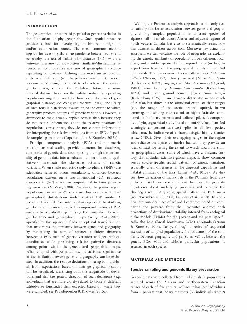
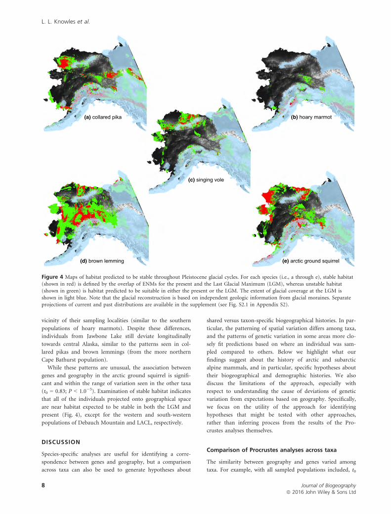
Figure 1 Sampled populations for the five mammal taxa in Alaska: collared pika (Ochotona collaris), hoary marmot (Marmota caligata),
singing vole (Microtus miurus), brown lemming (Lemmus trimucronatus) and arctic ground squirrel (Spermophilus parryii). Also markedare the primary mountain ranges and uplands against a grey scale background. The sampling locations are representative of each
species’ range within the study area. The extent of overlap of their respective ranges differs; for example, collared pikas and hoarymarmots do not occur in northern Alaska (e.g. the Brooks Range). Overlapping sampling points indicate species were collected from the
same site. Photos credits: Moose Peterson (collared pika), Ivan Andrijevic (brown lemming), Link Olson (arctic ground squirrel),Jonathan L. Fiely (hoary marmot) and Creative Commons (singing vole).
Journal of Biogeographyª 2016 John Wiley & Sons Ltd
3
Generating biogeographical hypotheses for Alaskan alpine small mammals
required before the locus was processed was rounded up
(e.g. a locus would need to be genotyped in three out of five
individuals with r = 0.50).
Quantitative comparison of the similarity between
genes and geography
Principal components analyses were performed on cus-
tomized structure files. To create these files, the loci names
exported from the MySQL databases (see above) were used
as a ‘whitelist’ by the populations program in Stacks; in
order to stop populations from filtering out loci from our
data set (we wanted all of the data irrespective of the num-
ber of populations a locus occurred in or the number of
individuals a locus was present in within a population), we
set all parameters to 0. populations wrote the genomic data
in a Variant Call Format (vcf) file, which we converted to a
structure file format using PGDSpider 2.0.7.2 (Lischer &
Excoffier, 2012). The structure file for each species was
edited to exclude linked SNPs, as well as SNPs and individu-
als that contained a high proportion of missing data, which
can disproportionately affect patterns in a PCA (Wang et al.,
2012). First, all SNPs with > 70% missing data were deleted.
Next, the amount of missing data per individual was calcu-
lated, and individuals with prohibitively high amounts of
missing data (such that the final data set would contain too
few SNPs) were excluded (these individuals were obvious
because they generally contained > 90% missing data). The
final step was to maximize the number of SNPs and individ-
uals such that each individual had < 15% missing data (Lis-
cher & Excoffier, 2012); the final number of individuals used
in subsequent analyses is presented in Table S1.1 in
Appendix S1.
Principal components analysis were performed on species-
specific matrices in R (R Core Team, 2014) using the
Adegenet R package (Jombart et al., 2008). Missing data
were replaced by the mean frequency of the corresponding
allele, which is recommended for centred PCAs (Jombart
et al., 2008). Major axes for genome-wide SNP data were
identified using the R Dudi.pca function (centre = T,
scale = T). An association between genetic differentiation and
geography was assessed considering divergence along both lat-
itudinal and longitudinal axes across populations using a Pro-
crustes transformation approach. Specifically, species-specific
PC1 and PC2 scores and the projected latitude and longitude
of sampling localities were inputs in a Procrustes analysis,
which maximizes the similarity between PCA maps of genetic
variation and geographical locations of sampled populations
(see Wang et al., 2010, 2012). Geographical coordinates were
transformed to an Albers Equal Area Conic projection using
the spTransform function in the rgdal R package (Bivand
et al., 2014). Analyses were performed using the protest
function in the vegan R package (Oksanen et al., 2013).
Because Procrustes analysis superimposes a PCA plot of
genetic variation onto a geographical map by rotating the PC
axes to achieve maximum similarity to the geographical dis-
tribution of sampled locations (i.e. the sum of squared differ-
ences between the two data sets are minimized), it is ideal for
quantitative comparison of the similarity between genes and
geography across taxa (as it is for comparing the association
between regions; see Wang et al., 2010). We report the angle
of the PCA map (i.e. h, the rotation measured in degrees)
that optimally minimizes the sum of squared Euclidean dis-
tance between the PCA map from the SNP data and the geo-
graphical map. The significance of the association statistic
between the first two PCs of genetic variation and the geo-
graphical coordinates of the populations (denoted as t0) for
each species was evaluated based on 10,000 permutations,
where geographical locations were randomly permuted across
the different sample localities (note that all individuals from
the same locality were assigned to a single geographical loca-
tion in the permuted data set, such that observed levels of
population structure were maintained).
As the aim of the work was to evaluate the overall simi-
larity (or lack thereof) in the association between genes and
geography across taxa, we assessed the robustness of our
results by excluding one population at a time and repeating
the PCA and Procrustes analyses on the new data sets. Com-
parison of the PCA coordinates from the new data sets and
the original geographical data sets were applied systemati-
cally to identify the maximum extent to which the associa-
tion between genes and geography might increase or
decrease as different populations were excluded, denoted by
the similarity score t″ (following the notation of Wang
et al., 2012). In addition, a similarity score denoted by t0
(following the notation of Wang et al., 2012) was computed
between the new PCA coordinates for the SNP data and the
original PCA coordinates for the SNP data (i.e. before
removing any population) to assess how robust the patterns
among populations in PCA space are to individual popula-
tions.
Environmental niche modelling
Environmental niche models (ENMs) were generated from
bioclimatic variables for the present and the LGM with Max-
ent 3.3.3e (Phillips et al., 2006). We performed a priori
model testing to determine optimal combinations of the reg-
ularization and feature parameters for the construction of
each species’ present-day ENM (Warren & Seifert, 2011).
Specifically, we used SDMToolBox (Brown, 2014) to test
models over combinations of regularization parameters from
0.25 to 3 in intervals of 0.25 and the Linear, Quadratic,
Hinge, Product and Threshold features. Each model parame-
ter class was replicated 25 times using cross-validation. Geo-
referenced distribution points from vetted occurrence data
used in the modelling were representative of the entire
ranges of the five species, respectively, throughout north-
western North America (Dryad doi:10.5061/dryad.8jm51).
For each species, occurrence data were spatially rarefied using
SDMToolBox at a resolution of 10 km to reduce spatial
autocorrelation.
Journal of Biogeographyª 2016 John Wiley & Sons Ltd
4
L. L. Knowles et al.
We used 19 bioclimatically informative variables to model
present-day distributions (WorldClim 1.4; Hijmans et al.,
2005) and LGM distributions (PMIP2-CCSM; Braconnot
et al., 2007) for each species. To avoid overfitting of the dis-
tribution models, the geographical extent of the environmen-
tal layers was reduced to an area c. 20% larger than the
known distribution of each species (Anderson & Raza, 2010)
and coupled with background sampling bias files (Phillips
et al., 2009; Merow et al., 2013). Sampling bias files were
constructed in SDMToolBox using a buffer distance of
100 km, which was reasonable given the geographical extent
of Alaska and the distance among species’ occurrence points.
Subsequently, the following procedure was carried out for
each species to guard against the inherent difficulties in
extrapolating distributions into novel climates (reviewed in
Alvarado-Serrano & Knowles, 2014). Specifically, an iterative
approach was used to generate ENMs for the LGM in which
multivariate environmental similarity surfaces (MESS maps)
were used to identify bioclimatic variables that result in areas
of low reliability because of predicted values that are outside
of the range of present-day environmental values for any
given taxon (Elith et al., 2010). Maxent was rerun excluding
these out-of-range variables, and this process of analysis with
MESS maps was repeated until no LGM variables were out-
of-range compared to present-day bioclimatic variables.
Because MESS maps do not indicate changes in correlations
among the environmental variables used for LGM recon-
structions (Elith et al., 2010), we checked our ENM for the
LGM using only the most informative variable for each spe-
cies to ensure that we were not reporting errant distribu-
tional patterns. In addition, a present-day ENM was
generated using the subset of variables that were not out-of-
range during the LGM and compared to an ENM con-
structed using the most important variable (as determined
by Maxent) and the remaining variables that had Pearson’s
r correlations to this variable of < 90%, as determined by
ENMTools (Warren et al., 2010); while these models were
not expected to be identical, we checked that both models
reported similar distributional patterns. Details about spe-
cies-specific environmental variables and parameters for the
different models are reported in Table S2.1 in Appendix S2.
RESULTS
Sequence data and genetic diversity
More than 500-million reads were produced across the four
lanes of Illumina sequencing (average of
1,821,116 � 825,584 reads per analysed individual across
species; for details see Table S1.2 in Appendix S1). After
excluding SNPs that were linked and/or that had greater than
15% missing data, the number of independent SNPs per spe-
cies was: collared pika, 7463; hoary marmot, 5524; singing
vole, 3666; brown lemming, 4718; arctic ground squirrel,
3502 (note that variation in the number of SNPs primarily
reflects differences in genome size and effective population
size across taxa, given the similar quality of reads, and the
number and distribution of reads across specimens, in each
library). Summaries of genetic diversity per population are
given for each of the five taxa in Table S3.1 in Appendix S3.
Heterozygosity was generally consistent across populations
(with the exception of the Sud Island population of the
hoary marmot, which had a considerably lower observed
heterozygosity compared to other populations), but differed
among taxa.
Procrustes analyses and ENMs
We find significant similarity between genes and geography
across taxa (see Table S3.2 in Appendix S3). However, the
strength of similarity differs among taxa and across geo-
graphical regions (see Fig. S3.2 in Appendix S3). Below we
describe these associations between genes and geography on
a per-species basis, including the robustness of the associa-
tion with the exclusion of populations, as well as how the
results from the Procrustes analyses conform to the projec-
tions of the species’ distributions in the past based on the
ENMs.
Collared pika
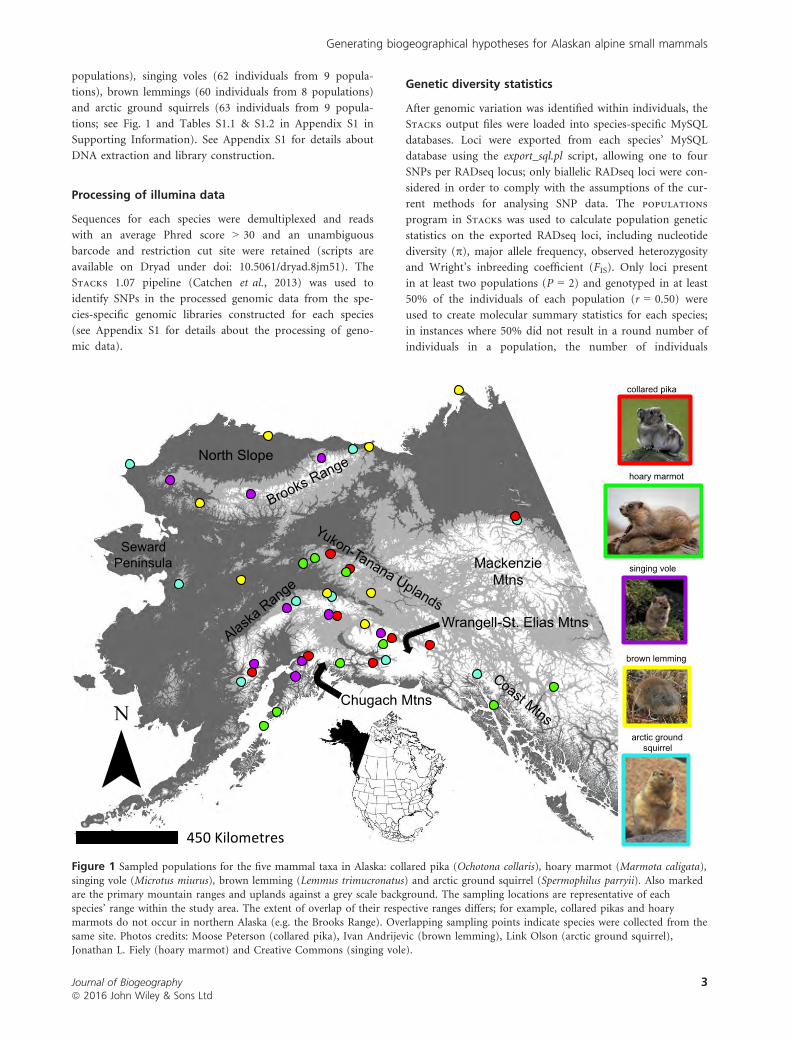
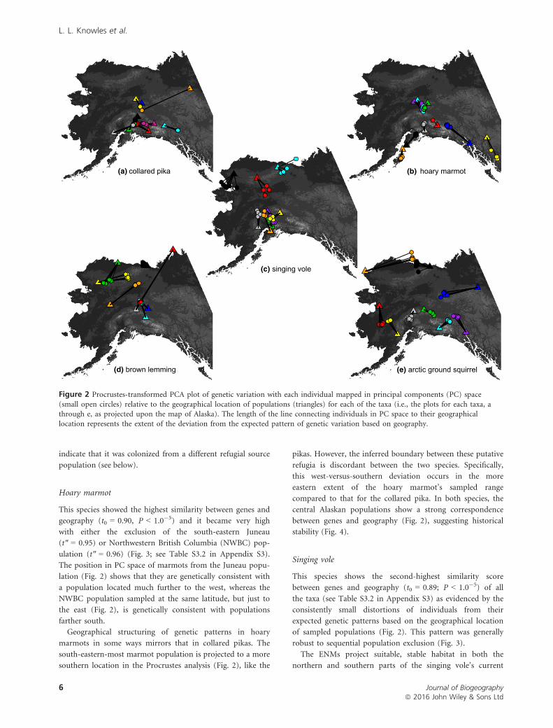
Although the similarity score between the pika populations
in PC space and their actual geographical locations is signifi-
cant (t0 = 0.71; P < 1.0�5), t0 is generally low compared to
other taxa (only the brown lemming has a lower t0). This is
in part due to departures associated with Jawbone Lake and
the Pika Camp populations. For example, given the distance
from Jawbone Lake in the east to Lake Kenibuna in the west,
we would expect a large distribution of genetic variation
along the longitudinal axis. Instead, individuals from these
populations cluster with individuals from more centrally
located populations (Fig. 2 and Fig. S3.1 in Appendix S3). In
contrast, the Pika Camp population is more divergent geneti-
cally than would be predicted by geography alone (i.e. the
population occupies a more distant area of PC space relative
to the other populations).
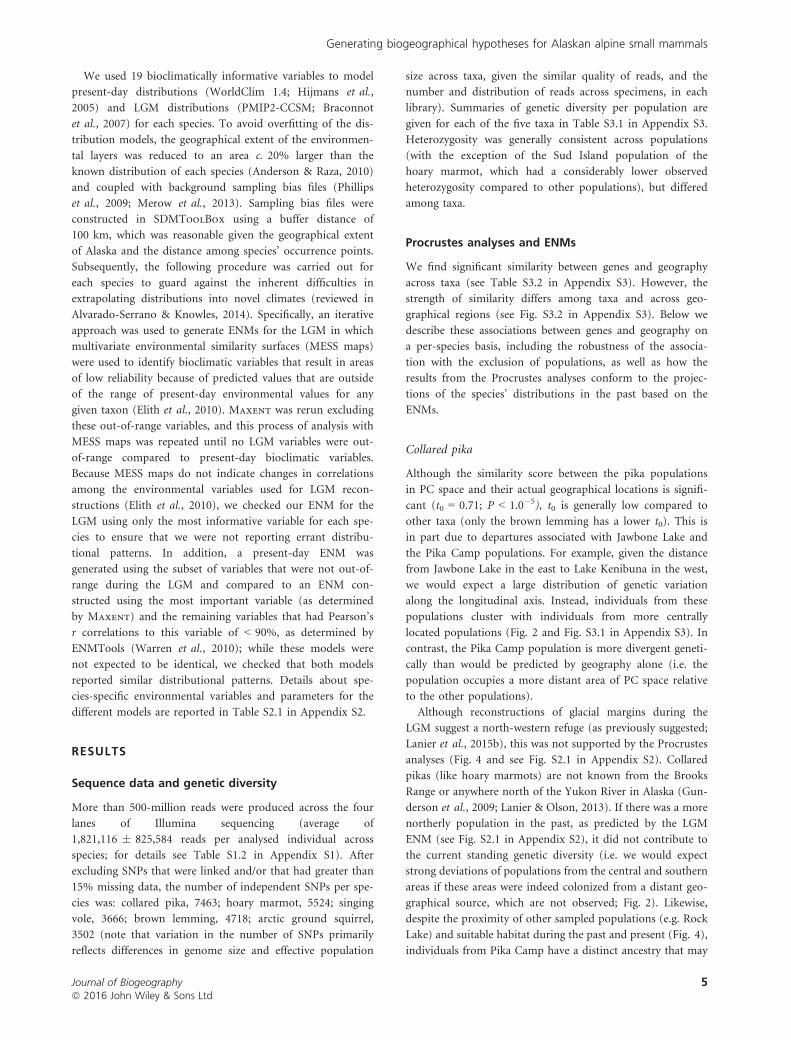
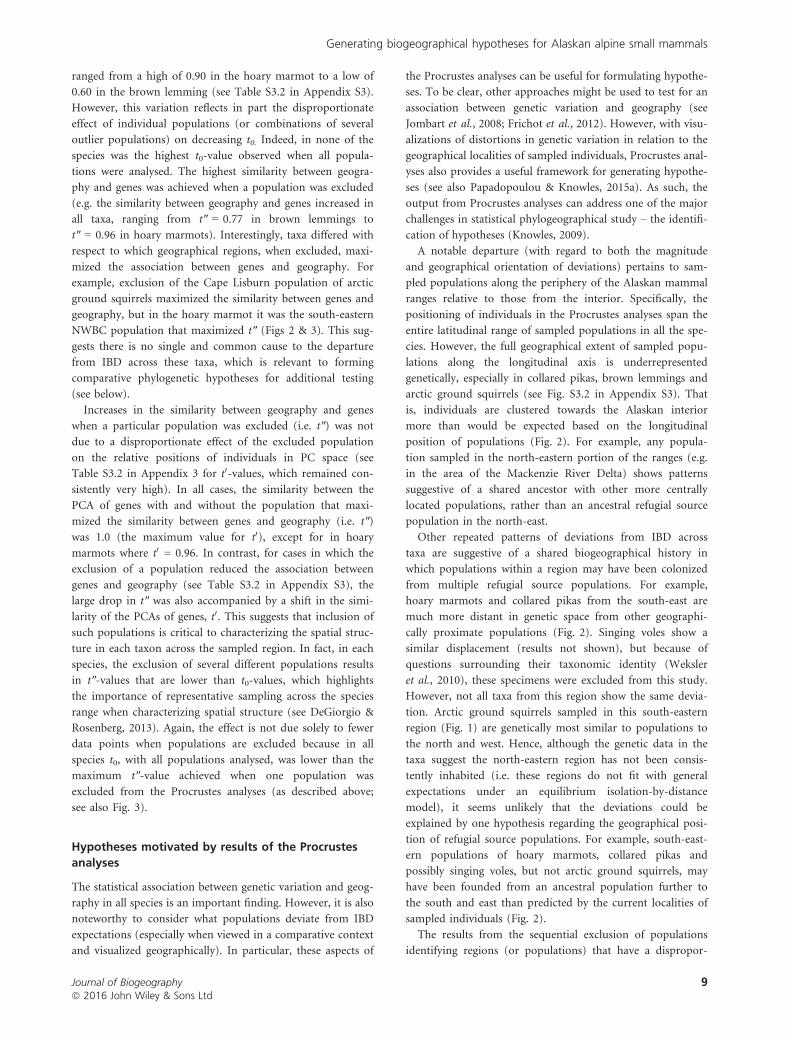
Although reconstructions of glacial margins during the
LGM suggest a north-western refuge (as previously suggested;
Lanier et al., 2015b), this was not supported by the Procrustes
analyses (Fig. 4 and see Fig. S2.1 in Appendix S2). Collared
pikas (like hoary marmots) are not known from the Brooks
Range or anywhere north of the Yukon River in Alaska (Gun-
derson et al., 2009; Lanier & Olson, 2013). If there was a more
northerly population in the past, as predicted by the LGM
ENM (see Fig. S2.1 in Appendix S2), it did not contribute to
the current standing genetic diversity (i.e. we would expect
strong deviations of populations from the central and southern
areas if these areas were indeed colonized from a distant geo-
graphical source, which are not observed; Fig. 2). Likewise,
despite the proximity of other sampled populations (e.g. Rock
Lake) and suitable habitat during the past and present (Fig. 4),
individuals from Pika Camp have a distinct ancestry that may
Journal of Biogeographyª 2016 John Wiley & Sons Ltd
5
Generating biogeographical hypotheses for Alaskan alpine small mammals
indicate that it was colonized from a different refugial source
population (see below).
Hoary marmot
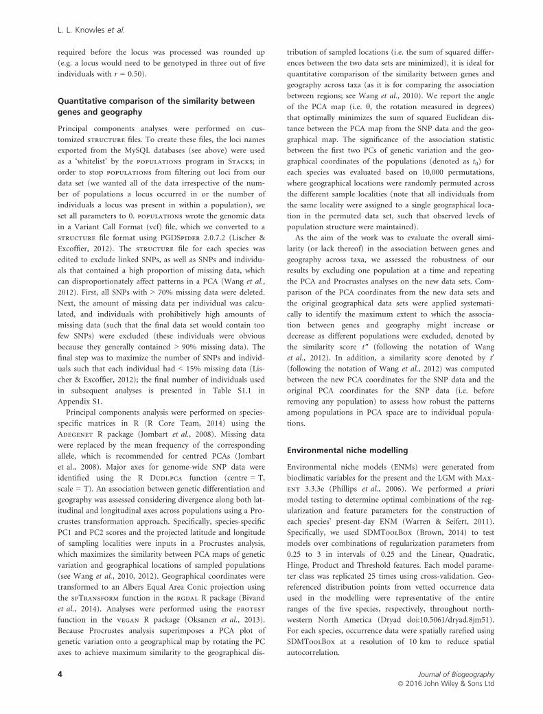
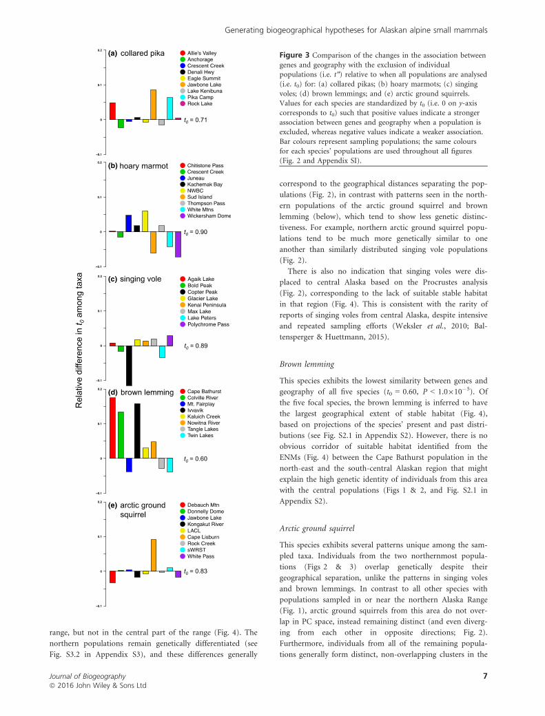
This species showed the highest similarity between genes and
geography (t0 = 0.90, P < 1.0�5) and it became very high
with either the exclusion of the south-eastern Juneau
(t″ = 0.95) or Northwestern British Columbia (NWBC) pop-
ulation (t″ = 0.96) (Fig. 3; see Table S3.2 in Appendix S3).
The position in PC space of marmots from the Juneau popu-
lation (Fig. 2) shows that they are genetically consistent with
a population located much further to the west, whereas the
NWBC population sampled at the same latitude, but just to
the east (Fig. 2), is genetically consistent with populations
farther south.
Geographical structuring of genetic patterns in hoary
marmots in some ways mirrors that in collared pikas. The
south-eastern-most marmot population is projected to a more
southern location in the Procrustes analysis (Fig. 2), like the
pikas. However, the inferred boundary between these putative
refugia is discordant between the two species. Specifically,
this west-versus-southern deviation occurs in the more
eastern extent of the hoary marmot’s sampled range
compared to that for the collared pika. In both species, the
central Alaskan populations show a strong correspondence
between genes and geography (Fig. 2), suggesting historical
stability (Fig. 4).
Singing vole
This species shows the second-highest similarity score
between genes and geography (t0 = 0.89; P < 1.0�5) of all
the taxa (see Table S3.2 in Appendix S3) as evidenced by the
consistently small distortions of individuals from their
expected genetic patterns based on the geographical location
of sampled populations (Fig. 2). This pattern was generally
robust to sequential population exclusion (Fig. 3).
The ENMs project suitable, stable habitat in both the
northern and southern parts of the singing vole’s current
(d) brown lemming
(b) hoary marmot
(c) singing vole
(a) collared pika
(e) arctic ground squirrel
Figure 2 Procrustes-transformed PCA plot of genetic variation with each individual mapped in principal components (PC) space
(small open circles) relative to the geographical location of populations (triangles) for each of the taxa (i.e., the plots for each taxa, athrough e, as projected upon the map of Alaska). The length of the line connecting individuals in PC space to their geographical
location represents the extent of the deviation from the expected pattern of genetic variation based on geography.
Journal of Biogeographyª 2016 John Wiley & Sons Ltd
6
L. L. Knowles et al.
range, but not in the central part of the range (Fig. 4). The
northern populations remain genetically differentiated (see
Fig. S3.2 in Appendix S3), and these differences generally
correspond to the geographical distances separating the pop-
ulations (Fig. 2), in contrast with patterns seen in the north-
ern populations of the arctic ground squirrel and brown
lemming (below), which tend to show less genetic distinc-
tiveness. For example, northern arctic ground squirrel popu-
lations tend to be much more genetically similar to one
another than similarly distributed singing vole populations
(Fig. 2).
There is also no indication that singing voles were dis-
placed to central Alaska based on the Procrustes analysis
(Fig. 2), corresponding to the lack of suitable stable habitat
in that region (Fig. 4). This is consistent with the rarity of
reports of singing voles from central Alaska, despite intensive
and repeated sampling efforts (Weksler et al., 2010; Bal-
tensperger & Huettmann, 2015).
Brown lemming
This species exhibits the lowest similarity between genes and
geography of all five species (t0 = 0.60, P < 1.0910�5). Of
the five focal species, the brown lemming is inferred to have
the largest geographical extent of stable habitat (Fig. 4),
based on projections of the species’ present and past distri-
butions (see Fig. S2.1 in Appendix S2). However, there is no
obvious corridor of suitable habitat identified from the
ENMs (Fig. 4) between the Cape Bathurst population in the
north-east and the south-central Alaskan region that might
explain the high genetic identity of individuals from this area
with the central populations (Figs 1 & 2, and Fig. S2.1 in
Appendix S2).
Arctic ground squirrel
This species exhibits several patterns unique among the sam-
pled taxa. Individuals from the two northernmost popula-
tions (Figs 2 & 3) overlap genetically despite their
geographical separation, unlike the patterns in singing voles
and brown lemmings. In contrast to all other species with
populations sampled in or near the northern Alaska Range
(Fig. 1), arctic ground squirrels from this area do not over-
lap in PC space, instead remaining distinct (and even diverg-
ing from each other in opposite directions; Fig. 2).
Furthermore, individuals from all of the remaining popula-
tions generally form distinct, non-overlapping clusters in the
(a)
(b)
(c)
(d)
(e)
Figure 3 Comparison of the changes in the association between
genes and geography with the exclusion of individualpopulations (i.e. t″) relative to when all populations are analysed
(i.e. t0) for: (a) collared pikas; (b) hoary marmots; (c) singing
voles; (d) brown lemmings; and (e) arctic ground squirrels.Values for each species are standardized by t0 (i.e. 0 on y-axis
corresponds to t0) such that positive values indicate a strongerassociation between genes and geography when a population is
excluded, whereas negative values indicate a weaker association.Bar colours represent sampling populations; the same colours
for each species’ populations are used throughout all figures(Fig. 2 and Appendix SI).
Journal of Biogeographyª 2016 John Wiley & Sons Ltd
7
Generating biogeographical hypotheses for Alaskan alpine small mammals
vicinity of their sampling localities (similar to the southern
populations of hoary marmots). Despite these differences,
individuals from Jawbone Lake still deviate longitudinally
towards central Alaska, similar to the patterns seen in col-
lared pikas and brown lemmings (from the more northern
Cape Bathurst population).
While these patterns are unusual, the association between
genes and geography in the arctic ground squirrel is signifi-
cant and within the range of variation seen in the other taxa
(t0 = 0.83; P < 1.0�5). Examination of stable habitat indicates
that all of the individuals projected onto geographical space
are near habitat expected to be stable in both the LGM and
present (Fig. 4), except for the western and south-western
populations of Debauch Mountain and LACL, respectively.
DISCUSSION
Species-specific analyses are useful for identifying a corre-
spondence between genes and geography, but a comparison
across taxa can also be used to generate hypotheses about
shared versus taxon-specific biogeographical histories. In par-
ticular, the patterning of spatial variation differs among taxa,
and the patterns of genetic variation in some areas more clo-
sely fit predictions based on where an individual was sam-
pled compared to others. Below we highlight what our
findings suggest about the history of arctic and subarctic
alpine mammals, and in particular, specific hypotheses about
their biogeographical and demographic histories. We also
discuss the limitations of the approach, especially with
respect to understanding the cause of deviations of genetic
variation from expectations based on geography. Specifically,
we focus on the utility of the approach for identifying
hypotheses that might be tested with other approaches,
rather than inferring process from the results of the Pro-
crustes analyses themselves.
Comparison of Procrustes analyses across taxa
The similarity between geography and genes varied among
taxa. For example, with all sampled populations included, t0
(d) brown lemming
(b) hoary marmot
(c) singing vole
(a) collared pika
(e) arctic ground squirrel
Figure 4 Maps of habitat predicted to be stable throughout Pleistocene glacial cycles. For each species (i.e., a through e), stable habitat
(shown in red) is defined by the overlap of ENMs for the present and the Last Glacial Maximum (LGM), whereas unstable habitat(shown in green) is habitat predicted to be suitable in either the present or the LGM. The extent of glacial coverage at the LGM is
shown in light blue. Note that the glacial reconstruction is based on independent geologic information from glacial moraines. Separateprojections of current and past distributions are available in the supplement (see Fig. S2.1 in Appendix S2).
Journal of Biogeographyª 2016 John Wiley & Sons Ltd
8
L. L. Knowles et al.
ranged from a high of 0.90 in the hoary marmot to a low of
0.60 in the brown lemming (see Table S3.2 in Appendix S3).
However, this variation reflects in part the disproportionate
effect of individual populations (or combinations of several
outlier populations) on decreasing t0. Indeed, in none of the
species was the highest t0-value observed when all popula-
tions were analysed. The highest similarity between geogra-
phy and genes was achieved when a population was excluded
(e.g. the similarity between geography and genes increased in
all taxa, ranging from t″ = 0.77 in brown lemmings to
t″ = 0.96 in hoary marmots). Interestingly, taxa differed with
respect to which geographical regions, when excluded, maxi-
mized the association between genes and geography. For
example, exclusion of the Cape Lisburn population of arctic
ground squirrels maximized the similarity between genes and
geography, but in the hoary marmot it was the south-eastern
NWBC population that maximized t″ (Figs 2 & 3). This sug-
gests there is no single and common cause to the departure
from IBD across these taxa, which is relevant to forming
comparative phylogenetic hypotheses for additional testing
(see below).
Increases in the similarity between geography and genes
when a particular population was excluded (i.e. t″) was not
due to a disproportionate effect of the excluded population
on the relative positions of individuals in PC space (see
Table S3.2 in Appendix 3 for t0-values, which remained con-
sistently very high). In all cases, the similarity between the
PCA of genes with and without the population that maxi-
mized the similarity between genes and geography (i.e. t″)
was 1.0 (the maximum value for t0), except for in hoary
marmots where t0 = 0.96. In contrast, for cases in which the
exclusion of a population reduced the association between
genes and geography (see Table S3.2 in Appendix S3), the
large drop in t″ was also accompanied by a shift in the simi-
larity of the PCAs of genes, t0. This suggests that inclusion of
such populations is critical to characterizing the spatial struc-
ture in each taxon across the sampled region. In fact, in each
species, the exclusion of several different populations results
in t″-values that are lower than t0-values, which highlights
the importance of representative sampling across the species
range when characterizing spatial structure (see DeGiorgio &
Rosenberg, 2013). Again, the effect is not due solely to fewer
data points when populations are excluded because in all
species t0, with all populations analysed, was lower than the
maximum t″-value achieved when one population was
excluded from the Procrustes analyses (as described above;
see also Fig. 3).
Hypotheses motivated by results of the Procrustes
analyses
The statistical association between genetic variation and geog-
raphy in all species is an important finding. However, it is also
noteworthy to consider what populations deviate from IBD
expectations (especially when viewed in a comparative context
and visualized geographically). In particular, these aspects of
the Procrustes analyses can be useful for formulating hypothe-
ses. To be clear, other approaches might be used to test for an
association between genetic variation and geography (see
Jombart et al., 2008; Frichot et al., 2012). However, with visu-
alizations of distortions in genetic variation in relation to the
geographical localities of sampled individuals, Procrustes anal-
yses also provides a useful framework for generating hypothe-
ses (see also Papadopoulou & Knowles, 2015a). As such, the
output from Procrustes analyses can address one of the major
challenges in statistical phylogeographical study – the identifi-
cation of hypotheses (Knowles, 2009).
A notable departure (with regard to both the magnitude
and geographical orientation of deviations) pertains to sam-
pled populations along the periphery of the Alaskan mammal
ranges relative to those from the interior. Specifically, the
positioning of individuals in the Procrustes analyses span the
entire latitudinal range of sampled populations in all the spe-
cies. However, the full geographical extent of sampled popu-
lations along the longitudinal axis is underrepresented
genetically, especially in collared pikas, brown lemmings and
arctic ground squirrels (see Fig. S3.2 in Appendix S3). That
is, individuals are clustered towards the Alaskan interior
more than would be expected based on the longitudinal
position of populations (Fig. 2). For example, any popula-
tion sampled in the north-eastern portion of the ranges (e.g.
in the area of the Mackenzie River Delta) shows patterns
suggestive of a shared ancestor with other more centrally
located populations, rather than an ancestral refugial source
population in the north-east.
Other repeated patterns of deviations from IBD across
taxa are suggestive of a shared biogeographical history in
which populations within a region may have been colonized
from multiple refugial source populations. For example,
hoary marmots and collared pikas from the south-east are
much more distant in genetic space from other geographi-
cally proximate populations (Fig. 2). Singing voles show a
similar displacement (results not shown), but because of
questions surrounding their taxonomic identity (Weksler
et al., 2010), these specimens were excluded from this study.
However, not all taxa from this region show the same devia-
tion. Arctic ground squirrels sampled in this south-eastern
region (Fig. 1) are genetically most similar to populations to
the north and west. Hence, although the genetic data in the
taxa suggest the north-eastern region has not been consis-
tently inhabited (i.e. these regions do not fit with general
expectations under an equilibrium isolation-by-distance
model), it seems unlikely that the deviations could be
explained by one hypothesis regarding the geographical posi-
tion of refugial source populations. For example, south-east-
ern populations of hoary marmots, collared pikas and
possibly singing voles, but not arctic ground squirrels, may
have been founded from an ancestral population further to
the south and east than predicted by the current localities of
sampled individuals (Fig. 2).
The results from the sequential exclusion of populations
identifying regions (or populations) that have a dispropor-
Journal of Biogeographyª 2016 John Wiley & Sons Ltd
9
Generating biogeographical hypotheses for Alaskan alpine small mammals
tionate effect on the association between genes and geogra-
phy can also be a source of information for developing
hypotheses about region-specific processes. For example, a
much higher association between genes and geography
results when brown lemmings from northern coastal popula-
tions (Fig. 2) are excluded in Procrustes analyses (Fig. 3).
This suggests that a possible hypothesis to explain the devia-
tions between genes and geography in brown lemmings
(Fig. 2) would have to accommodate the entire northern
coastal region (not just one or two specific populations).
Moreover, latitudinal differences in the genetic similarity of
individuals suggest the region might have experienced fairly
localized processes. These might include aspects of the
demography of colonization and/or different ancestral source
populations (i.e. individuals from Cape Bathurst and Colville
River show genetic variation consistent with individuals sam-
pled from more southern latitudes, in contrast to the Ivvavik
population).
This more nuanced picture with concordance limited to
specific taxa and certain geographical regions differs from
more generalized hypotheses identified from mtDNA (Gal-
breath et al., 2011; Lanier et al., 2015a). Perhaps this is not
entirely unexpected given that different markers provide dif-
fering degrees of resolution (Knowles, 2009). With the addi-
tional resolution of genomic markers it is increasingly clear
that relying on mtDNA (or any single linkage partition) alone
overlooks processes that may actually structure genomic vari-
ation. For example, unlike interior Alaska, which was part of
ice-free Beringia during the LGM, formerly ice-covered locali-
ties within the hoary marmot’s current distribution show the
greatest discordance between genes and geography (i.e.
Figs 2b & 3b). Likewise, a rapid expansion of hoary marmots
from one or more south-central refugia (either nunataks or
periglacial areas predicted as being suitable marmot habitat
during the LGM; Fig. 4b) suggests a more dynamic history
than suggested by past studies. Nevertheless, the genomic
analyses also provide corroborative support for some species-
specific hypotheses suggested by patterns of mtDNA differen-
tiation. For example, a possible inland incursion from a
coastal refugium (see Kerhoulas et al., 2015) originating south
of our sampling regime is suggested by the seemingly anoma-
lous discordance in the NWBC marmots (Fig. 2).
Testing hypotheses developed from the findings of
the Procrustes analyses
Some hypotheses suggested by the Procrustes analyses appear
to be corroborated from independent data sources. For
example, we have hypothesized that the Yukon-Tanana
uplands are a potential refugium for hoary marmots and col-
lared pikas based on deformations in the north-central parts
of their range in the Procrustes analyses (Fig. 2). This area is
also projected to be highly suitable and stable habitat by the
ENMs (see Fig. S2.1 in Appendix S2), and it has been identi-
fied as a biodiversity hotspot for Alaskan small mammals
(Baltensperger & Huettmann, 2015).
More generally, and as we advocate here, departures from
IBD detected in the Procrustes analyses can be used to gener-
ate hypotheses for future study (as discussed above). How-
ever, the results from the Procrustes analyses, by themselves,
are not sufficient for interpreting the processes underlying
the lack of a correspondence between genes and geography
(see below).
Not only might different processes leave similar signatures
that can be difficult to distinguish, but the signal of a specific
process may not be easily intuited from the pattern of devia-
tions evident in the Procrustes plots, as with other summaries
of genetic variation (see Knowles & Alvarado-Serrano, 2010;
Brown & Knowles, 2012; He et al., 2013; Wang & Bradburd,
2014). For example, it is difficult to identify one hypothesis
that might have generated the deviations from IBD observed
in the arctic ground squirrel (Fig. 2). Only the exclusion of
the north-western population lead to an appreciable increase
in this association (Fig. 3), leaving a fair amount of genetic
variation that is not explained by IBD. A possible hypothesis
that might be considered is isolation by colonization in which
the populations were founded from a single centrally located
ancestral source. However, this model alone wouldn’t neces-
sarily explain why the southern populations show latitudinal
departures, but little deformation from longitudinal positions
of populations (Fig. 2). Perhaps a non-equilibrium model in
which the rate, or timing, of latitudinal spread differed from
the longitudinal spread in the south could generate the
observed deviations from IBD. Without further analysis, it is
not possible to evaluate the likelihood of such a hypothesis.
Such detailed demographic scenarios might be informed
directly from the ENMs (see Fig. S2.1 in Appendix S2),
including inferred areas of stability (Fig. 4), as with modelling
approaches like the iDDC (He et al., 2013). For example,
changes in the suitability of habitats across the landscape, and
changes in suitability over time, can be used to inform the
colonization process associated with shifting distributions dri-
ven by glacial cycles (Brown & Knowles, 2012).
In addition to the multiple processes that might generate a
departure from IBD, the magnitude and orientation of defor-
mations in the Procrustes plots (i.e. the length of the arrows;
see Fig. 2) may also be impacted by the timing of the events
that cause a departure between genes and geography (e.g.
Excoffier et al., 2009). For example, for a recent expansion
the direction of the deviations might be captured in a Pro-
crustes analysis, but a population near the site of an expan-
sion centre might show higher deviations relative to more
geographicalally distant populations if the expansion has
been recent (see simulation results in He et al., 2013). Like-
wise, because PCA can be sensitive to the sampling of indi-
viduals over geographical space (e.g. over- or under-
representative sampling for some regions; see DeGiorgio &
Rosenberg, 2013), it is possible that such effects could influ-
ence some of the Procrustes analyses. We note that in gen-
eral the patterns in the genetic PCs were not significantly
impacted when we excluded one population at a time (see
t0-values in Table S3.2 in Appendix S3). This suggests that
Journal of Biogeographyª 2016 John Wiley & Sons Ltd
10
L. L. Knowles et al.
results from analyses of the full Alaskan mammal data sets
considered here are not being biased by geographical uneven-
ness in the sampling of individuals. However, whether the
results from Procrustes analyses are robust to different sam-
ple sizes across space is not known.
Does this mean that the results from Procrustes analyses
have no utility for identifying the processes causing depar-
tures from IBD? Not at all – it just means that any interpre-
tation will have to take into to account the uncertainty that
would come with a single summary of genetic variation. For
example, the statistical summaries from the Procrustes analy-
ses (e.g. the t0, t0, and t″-values, as well as the angle of rota-
tion to maximize the covariance between genes and
geographical matrices) could provide valuable summary
statistics for incorporation into procedures like Approximate
Bayesian Computation (ABC) to test phylogeographical
hypotheses. Likewise, integrated models of phylodemographic
movements (e.g. iDCC; He et al., 2013) may be useful in
teasing apart these alternative hypotheses, especially if the
differences among species discovered here are indicative of
an interaction of species history and biology (e.g. Massatti &
Knowles, 2014; Papadopoulou & Knowles, 2015b). In partic-
ular, our results hint at a possible distinction between more
mesic species (such as brown lemmings) and more xeric spe-
cies (such as collared pikas and hoary marmots). Brown lem-
mings show little geographical concordance in terms of
direction of deformation relative to contemporary popula-
tions. For example, the projections onto geographical coordi-
nates based on patterns of genetic variation do not overlap
(i.e. individuals from populations form discrete clusters),
and there is no concerted direction of movement as would
be expected when previously glaciated habitat are colonized
(Fig. 2). Other work has suggested that this region was a
tundra mosaic (Elias et al., 1996; Anderson et al., 2004),
which may have contributed to the lack of uniformity in the
direction of deformation.
The Procrustes analyses are just the first step towards
identifying future studies of genomic variation. With respect
to this fascinating group of mammals, the lack of concordant
genomic variation suggests there is no single geographical
region in Alaska that has remained isolated geologically (i.e.
a region that has remained independent of other regions) or
ecologically (i.e. a barrier that prohibited historical gene flow
among populations). However, some repeated patterns of
variation across subsets of taxa in some parts of their ranges
suggest a role for shared processes operating at more local
geographical scales. Future tests will explore the hypotheses
generated here, and evaluate the relative roles of taxon-speci-
fic versus regional processes in structuring genomic variation
across these alpine small mammal communities.
ACKNOWLEDGEMENTS
This work was funded by NSF (DEB 1118815 to L.L.K.,
DDIG DEB 0808619 to L.E.O. and H.C.L.) and the Alaska
Department of Fish and Game (State Wildlife Grants T-1-6,
T-3-6, and T-9-1 to L.E.O.). We are also grateful to the more
than 60 collectors without whose efforts this study would
not have been possible.
REFERENCES
Alvarado-Serrano, D.F. & Knowles, L.L. (2014) Environmen-
tal niche models in phylogeographic studies: recent
advances and precautions. Molecular Ecology Resources, 14,
233–248.Anderson, R.P. & Raza, A. (2010) The effect of the extent of
the study region on GIS models of species geographic dis-
tributions and estimates of niche evolution: preliminary
tests with montane rodents (genus Nephelomys) in Vene-
zuela. Journal of Biogeography, 37, 1378–1393.Anderson, P.M., Edwards, M.E. & Brubaker, L.B. (2004)
Results and paleoclimate implications of 35 years of pale-
oecological research in Alaska. Developments in Quaternary
Science (ed. by A.R. Gillespie, S.C. Porter and B.F. Atwa-
ter), pp. 427–440. Elsevier, London.Baltensperger, A.P. & Huettmann, F. (2015) Predictive spatial
niche and biodiversity hotspot models for small mammal
communities in Alaska: applying machine-learning to con-
servation planning. Landscape Ecology, 30, 681–697.Bivand, R., Keitt, T. & Rowlingson, B. (2014) rgdal: bindings
for the geospatial data abstraction library. R package ver-
sion 0.9-1. Available at: http://CRAN.R-project.org/packa-
ge=rgdal.
Braconnot, P., Otto-Bliesner, B., Harrison, S. et al. (2007)
Results of PMIP2 coupled simulations of the Mid-Holo-
cene and Last Glacial Maximum—part 1: experiments and
large-scale features. Climate of the Past, 3, 261–277.Brown, J.L. (2014) SDMtoolbox: a python-based GIS toolkit
for landscape genetic, biogeographic and species distribu-
tion model analyses. Methods in Ecology and Evolution, 5,
694–700.Brown, J.L. & Knowles, L.L. (2012) Spatially explicit models
of dynamic histories: examination of the genetic conse-
quences of Pleistocene glaciation and recent climate
change on the American Pika. Molecular Ecology, 21,
3757–3775.Catchen, J., Hohenlohe, P., Bassham, S., Amores, A. &
Cresko, W.A. (2013) Stacks: an analysis tool set for popu-
lation genomics. Molecular Ecology, 22, 3124–3140.DeGiorgio, M. & Rosenberg, N.A. (2013) Geographic sam-
pling scheme as a determinant of the major axis of genetic
variation in principal components analysis. Molecular Biol-
ogy and Evolution, 30, 480–488.Elias, S.A., Short, S.K., Nelson, C.H. & Birks, H.H. (1996) Life
and times of the Bering land bridge. Nature, 382, 60–62.Elith, J., Kearney, M. & Phillips, S. (2010) The art of mod-
elling range-shifting species. Methods in Ecology and Evolu-
tion, 1, 330–342.Excoffier, L., Foll, M. & Petit, R.J. (2009) Genetic conse-
quences of range expansions. Annual Review of Ecology
Evolution and Systematics, 40, 481–501.
Journal of Biogeographyª 2016 John Wiley & Sons Ltd
11
Generating biogeographical hypotheses for Alaskan alpine small mammals
Francois, O., Currat, M., Ray, N., Han, E., Excoffier, L. &
Novembre, J. (2010) Principal component analysis under
population genetic models of range expansion and admix-
ture. Molecular Biology and Evolution, 27, 1257–1268.Frichot, E., Schoville, S., Bouchard, G. & Franc�ois, O. (2012)
Correcting principal component maps for effects of spatial
autocorrelation in population genetic data. Frontiers in
Genetics, 3, e254.
Galbreath, K.E., Cook, J.A., Eddingsaas, A.A. & DeChaine,
E.G. (2011) Diversity and demography in Beringia: multilo-
cus tests of paleodistribution models reveal the complex his-
tory of Arctic ground squirrels. Evolution, 65, 1879–1896.Gunderson, A.M., Jacobsen, B.K. & Olson, L.E. (2009)
Revised distribution of the Alaska marmot, Marmota
broweri, and confirmation of parapatry with hoary mar-
mots. Journal of Mammalogy, 90, 859–869.He, Q., Edwards, D. & Knowles, L.L. (2013) Integrative test-
ing of how environments from the past to the present
shape genetic structure across landscapes. Evolution, 67,
3386–3402.Hijmans, R.J., Cameron, S.E., Parra, J.L., Jones, P.G. & Jarvis,
A. (2005) Very high resolution interpolated climate sur-
faces for global land areas. International Journal of Clima-
tology, 25, 1965–1978.Jombart, T., Devillard, S., Dufour, A. & Pontier, D. (2008)
Revealing cryptic spatial patterns in genetic variability by a
new multivariate method. Heredity, 101, 92–103.Kerhoulas, N.J., Gunderson, A.M. & Olson, L.E. (2015)
Complex history of isolation and gene flow in hoary,
Olympic, and endangered Vancouver Island marmots.
Journal of Mammalogy, 96, 810–826.Knowles, L.L. (2009) Statistical phylogeography. Annual
Review of Ecology Evolution and Systematics, 40, 593–612.Knowles, L.L. & Alvarado-Serrano, D.F. (2010) Exploring the
population genetic consequences of the colonization pro-
cess with spatio-temporally explicit models: insights from
coupled ecological, demographic, and genetic models in
montane grasshoppers. Molecular Ecology, 19, 3727–3745.Lanier, H.C. & Olson, L.E. (2013) Deep barriers, shallow
divergences: reduced phylogeographical structure in the
collared pika (Mammalia: Lagomorpha: Ochotona collaris).
Journal of Biogeography, 40, 466–478.Lanier, H.C., Gunderson, A.M., Weksler, M., Fedorov, V.B.
& Olson, L.E. (2015a) Comparative phylogeography of
eastern Beringian mammals highlights the double-edged
sword of climate change faced by arctic- and alpine-
adapted species. PLoS ONE, 10, e0118396.
Lanier, H.C., Massatti, R., He, Q., Olson, L.E. & Knowles,
L.L. (2015b) Colonization from divergent ancestors: glacia-
tion signatures on contemporary patterns of genetic varia-
tion in Collared Pikas (Ochotona collaris). Molecular
Ecology, 24, 3688–3705.Lischer, H.E.L. & Excoffier, L. (2012) PGDSpider: an auto-
mated data conversion tool for connecting population genet-
ics and genomics programs. Bioinformatics, 28, 298–299.
Massatti, R. & Knowles, L.L. (2014) Microhabitat differ-
ences impact phylogeographic concordance of co-distrib-
uted species: genomic evidence in montane sedges
(Carex L.) from the Rocky Mountains. Evolution, 68,
2833–2846.McVean, G. (2009) A genealogical interpretation of principal
components analysis. PLoS Genetics, 5, e1000686.
Merow, C., Smith, M.J. & Silander, J.A. (2013) A practical
guide to MaxEnt for modeling species’ distributions: what
it does, and why inputs and settings matter. Ecography, 36,
1058–1069.Novembre, J., Johnson, T., Bryc, K., Kutalik, Z., Boyko, A.R.,
Auton, A., Indap, A., King, K.S., Bergmann, S., Nelson,
M.R., Stephens, M. & Bustamante, C.D. (2008) Genes mir-
ror geography within Europe. Nature, 456, 98–101.Oksanen, J., Blanchet, F.G., Kindt, R., Legendre, P., Minchin,
P.R., O’Hara, R.B., Simpson, G.L., Solymos, P., Stevens,
M.H.H., Wagner, H. & Oksanen, J. (2013) Package Vegan.
Community ecology package. Version 2.0–10.Papadopoulou, A. & Knowles, L.L. (2015a) Species-specific
responses to island connectivity cycles: refined models for
testing phylogeographic concordance across a Mediter-
ranean Pleistocene Aggregate Island Complex. Molecular
Ecology, 24, 4252–4268.Papadopoulou, A. & Knowles, L.L. (2015b) Genomic tests of
the species-pump hypothesis: recent island connectivity
cycles drive divergence in Caribbean crickets across the
Virgin Islands. Evolution, 69, 1501–1517.Phillips, S.J., Anderson, R.P. & Schapire, R.E. (2006) Maxi-
mum entropy modeling of species geographic distribu-
tions. Ecological Modeling, 190, 231–259.Phillips, S.J., Dudik, M., Elith, J., Graham, C.H., Lehmann,
A., Leathwick, J. & Ferrier, S. (2009) Sample selection bias
and presence-only distribution models: implications for
background and pseudo-absence data. Ecological Applica-
tions, 19, 181–197.R Core Team (2014) R: A language and environment for sta-
tistical computing. R Foundation for Statistical Computing,
Vienna, Austria. Available at: http://www.R-project.org/.
(accessed 3 January 2015)
Wang, I.J. & Bradburd, G.S. (2014) Isolation by environ-
ment. Molecular Ecology, 23, 5649–5662.Wang, C., Szpiech, Z.A., Degnan, J.H., Jakobsson, M.,
Pemberton, T.J. et al. (2010) Comparing spatial maps of
human population-genetic variation using Procrustes anal-
ysis. Statical Applications in Genetics and Molecular Biology,
9, Article 13. doi: 10.2202/1544-6115.1493.
Wang, C., Z€ollner, S. & Rosenberg, N.A. (2012) A quantita-
tive comparison of the similarity between genes and geog-
raphy in worldwide human populations. PLoS Genetics, 8,
e1002886. doi:10.1371/journal.pgen.1002886.
Warren, D.L. & Seifert, S.N. (2011) Ecological niche model-
ing in Maxent: the importance of model complexity and
the performance of model selection criteria. Ecological
Applications, 21, 335–342.
Journal of Biogeographyª 2016 John Wiley & Sons Ltd
12
L. L. Knowles et al.
Warren, D.L., Glor, R.E. & Turelli, M. (2010) ENMTools: a
toolbox for comparative studies of environmental niche
models. Ecography, 33, 607–611.Weksler, M., Lanier, H.C. & Olson, L.E. (2010) Eastern
Beringian biogeography: historical and spatial genetic
structure of singing voles in Alaska. Journal of Biogeogra-
phy, 37, 1414–1431.
SUPPORTING INFORMATION
Additional Supporting Information may be found in the
online version of this article:
Appendix S1 Summaries of geographical information and
genomic sampling.
Appendix S2 Summaries of ENM settings and projections
of current and LGM distributions.
Appendix S3 PC maps of genetic variation and summaries
of genetic variation.
BIOSKETCH
L. Lacey Knowles and her lab are interested in understand-
ing the processes that structure patterns of genetic variation
across geographical landscapes and among taxa. Her lab
works on a diversity of empirical systems to discover how
species-specific responses to past events, especially those
caused by climate change, influence the connections among
populations that shape divergence patterns over space and
time. This work is also complemented by methodological
study and development to identify approaches that are useful
for making inferences about the processes that shape genetic
patterns within and among taxa.
Author contributions: L.L.K., Q.H. and R.M. conceived the
ideas; L.L.K. led the writing with input from all the other
co-authors; L.E.O. and H.C.L. collected the specimens;
H.C.L. and Q.H. collected the genomic data; Q.H. conducted
bioinformatics processing of genomic data; R.M. did the
genetic analyses and ENMs.
Editor: Brett Riddle
Journal of Biogeographyª 2016 John Wiley & Sons Ltd
13
Generating biogeographical hypotheses for Alaskan alpine small mammals
Knowles et al., Quantifying the similarity between genes and geography across Alaska’s alpine small mammals, Journal of biogeography. Appendix S1. Summaries of geographical information and genomic sampling Details about locality information (Table S1) and genomic data (Table S2) for sampled individuals are provided in this appendix, Appendix S1, along with details about library construction and processing. Genomic DNA was extracted from either fresh or frozen tissue using either Qiagen DNeasy or Gentra PureGene kits (Gentra Systems Inc., Minneapolis, MN, USA) following the manufacturer’s Animal Tissue Protocol. Four reduced-representation libraries were constructed using a restriction-fragment-based procedure (for details see Peterson et al., 2012). Within each library, individuals were doubly digested with the restriction enzymes EcoRI and MseI and uniquely tagged with a 10bp barcode. The digested products were then pooled and size-selected for 350-450bp fragments using a Pippin Prep (Sage Science, Beverly, MA, USA). Size-selected fragments were then amplified by PCR with iProof™ High-Fidelity DNA Polymerase (BIO-RAD). DNA quantification and cleaning with Agencourt AMPure XP (Beckman Coulter, Indianapolis, IN, USA) occurred after every step in the library construction procedure. Each genomic library was sequenced on an Illumina HiSeq2000 at the University of Michigan DNA Sequencing Core to generate 100bp paired-end reads; however, only the first read was retained here due to the need for unlinked single nucleotide polymorphisms (SNPs) in our analyses. The Stacks v1.07 pipeline (Catchen et al., 2013) was used to identify SNPs in the processed genomic data from the species-specific genomic libraries constructed for each species. Specifically, in each species-specific library, the USTACKS program was used to create a de novo assembly of reads with a minimum coverage depth (m = 3) into putative loci (i.e. into a “stack”). ‘RADseq locus/loci’ is hereafter used interchangeably with ‘locus/loci’ and refers to groups of 90 base-pair reads that are homologous (both within and among individuals); RADseq loci contain both invariable and variable DNA sites (i.e. SNPs). Reads were filtered using a removal algorithm that eliminated highly repetitive stacks (i.e. stacks that exceed the expected number of reads for a single locus given the average depth of coverage, for example, when loci are members of multi-gene families) and the ‘deleveraging algorithm’ to resolve over-merged loci (i.e. non-homologous loci misidentified as a single locus). SNPs were identified at each locus and genotypes were called using a multinomial-based likelihood model that accounts for sequencing error (Hohenlohe et al., 2010; Catchen et al., 2011; Catchen et al., 2013), with the upper bound of the error rate (ε) set to 0.1. A conservative upper bound was selected for ε, as these models have been developed primarily for higher-coverage data; a conservative bound was preferred over the unbounded model because the latter has been shown to underestimate heterozygotes (Catchen et al., 2013). A catalog of consensus loci among individuals was constructed with the CSTACKS program from the USTACKS output files using all of the individuals of each species. Loci were recognized as homologous across individuals if the distance between the consensus sequences (n) was ≤ 2. Each individual was matched against the catalog and alleles were identified in each individual using SSTACKS. A summary of the number of pre- and post-processing reads, as well as
the number utilized by Stacks, is given in Table S2 in this appendix. At this stage, 12 individuals with low coverage were excluded from further analyses (collared pika: 2, hoary marmot: 1, singing vole: 4, brown lemming: 3, arctic ground squirrel: 2; see Table S1 in this appendix); this first round of exclusions was based on those specimens with <35% of the reads utilized by Stacks (see Methods and Materials in main text for other processing steps). References Catchen, J.M., Amores, A., Hohenlohe, P., Cresko, W. & Postlethwait, J.H. (2011) Stacks: building and genotyping loci de novo from short-read sequences. G3: Genes, Genomes, Genetics, 1,171–182. Catchen, J., Hohenlohe, P., Bassham, S., Amores, A. & Cresko, W.A. (2013) Stacks: an analysis tool set for population genomics. Molecular Ecology, 22, 3124–3140. Hohenlohe, P.A., Phillips, P.C. & Cresko, W.A. (2010) Using population genomics to detect selection in natural populations: key concepts and methodological considerations. International Journal of Plant Sciences, 171, 1059–1071.
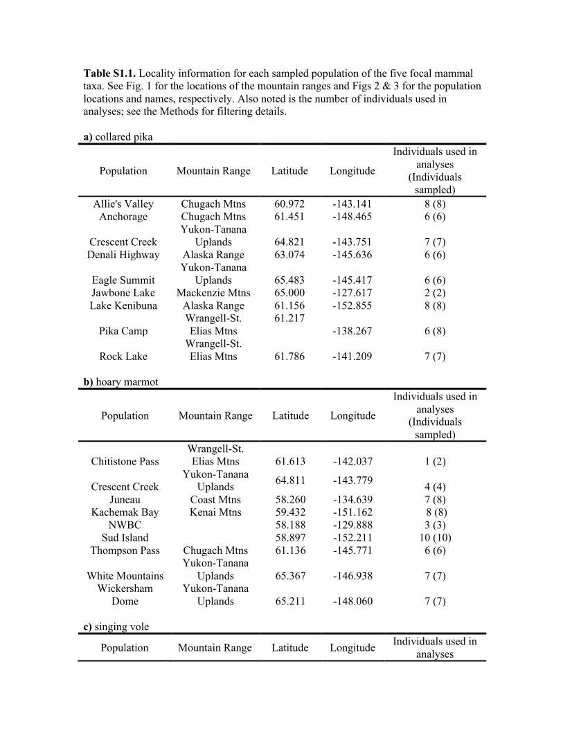
Table S1.1. Locality information for each sampled population of the five focal mammal taxa. See Fig. 1 for the locations of the mountain ranges and Figs 2 & 3 for the population locations and names, respectively. Also noted is the number of individuals used in analyses; see the Methods for filtering details. a) collared pika
Population Mountain Range Latitude Longitude
Individuals used in analyses
(Individuals sampled)
Allie's Valley Chugach Mtns 60.972 -143.141 8 (8) Anchorage Chugach Mtns 61.451 -148.465 6 (6)
Crescent Creek Yukon-Tanana
Uplands 64.821 -143.751 7 (7) Denali Highway Alaska Range 63.074 -145.636 6 (6)
Eagle Summit Yukon-Tanana
Uplands 65.483 -145.417 6 (6) Jawbone Lake Mackenzie Mtns 65.000 -127.617 2 (2) Lake Kenibuna Alaska Range 61.156 -152.855 8 (8)
Pika Camp Wrangell-St. Elias Mtns
61.217 -138.267 6 (8)
Rock Lake Wrangell-St. Elias Mtns 61.786 -141.209 7 (7)
b) hoary marmot
Population Mountain Range Latitude Longitude
Individuals used in analyses
(Individuals sampled)
Chitistone Pass Wrangell-St. Elias Mtns 61.613 -142.037 1 (2)
Crescent Creek Yukon-Tanana
Uplands 64.811 -143.779 4 (4) Juneau Coast Mtns 58.260 -134.639 7 (8)
Kachemak Bay Kenai Mtns 59.432 -151.162 8 (8) NWBC 58.188 -129.888 3 (3)
Sud Island 58.897 -152.211 10 (10) Thompson Pass Chugach Mtns 61.136 -145.771 6 (6)
White Mountains Yukon-Tanana
Uplands 65.367 -146.938 7 (7) Wickersham
Dome Yukon-Tanana
Uplands 65.211 -148.060 7 (7) c) singing vole
Population Mountain Range Latitude Longitude Individuals used in analyses
(Individuals sampled)
Agaik Lake Brooks Range 68.078 -152.921 4 (8) Bold Peak Chugach Mtns 61.365 -148.908 5 (5)
Chisana Wrangell-St. Elias Mtns 62.065 -142.046 0* (3)
Copter Peak Brooks Range 68.471 -161.478 7 (8) Glacier Lake Alaska Range 63.111 -146.247 4 (8)
Kenai Penninsula Kenai Mtns 60.782 -149.531 4 (6) Lake Peters Brooks Range 69.303 -145.025 6 (8) Max Lake Alaska Range 61.358 -152.869 7 (8)
Polychrome Pass Alaska Range 63.498 -149.886 6 (8) *Individuals from the Chisana population likely represent a different species and were not used in PCA analyses because they heavily influenced the relationships among the populations. d) brown lemming
Population Mountain Range Latitude Longitude
Individuals used in analyses
(Individuals sampled)
Cape Bathurst North coastline 70.500 -127.983 4 (4) Colville River North coastline 70.383 -150.800 7 (8)
Ivvavik National Park
North coastline 69.417 -139.600 6 (8)
Kaluich Creek Brooks Range 67.664 -158.191 6 (8) Mt. Fairplay Yukon-Tanana
Uplands 63.698 -142.255 8 (8)
Nowitna River Kuskokwim Mtns 64.685 -153.937 4 (8) Tangle Lakes Alaska Range 63.784 -145.785 9 (9) Twin Lakes Wrangell-St. Elias
Mtns 62.530 -143.258 7 (7)
e) arctic ground squirrel
Population Mountain Range Latitude Longitude
Individuals used in analyses
(Individuals sampled)
Cape Lisburn North coastline 68.871 -166.040 6 (7) Debauch Mountain
Nulato Hills 64.390 -159.656 8 (8)
Donnelly Dome Alaska Range 63.788 -145.800 4 (7) Jawbone Lake Mackenzie Mtns 64.817 -127.617 6 (8)
Kongakut River Brooks Range 69.449 -141.461 7 (8) LACL Alaska Range 60.654 -153.936 3 (4)

Rock Creek Alaska Range 63.750 -149.000 8 (8) sWRST Chugach Mtns 60.994 -142.029 7 (7)
White Pass Coast Mtns 59.616 -135.168 5 (6)
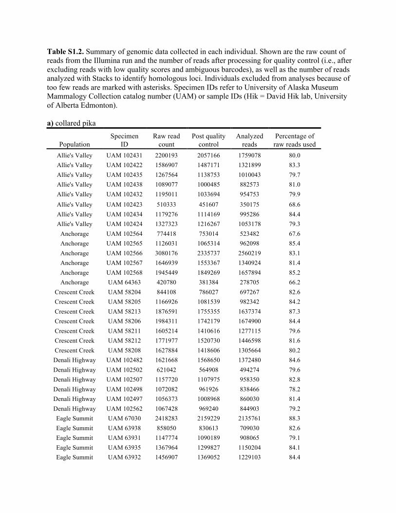
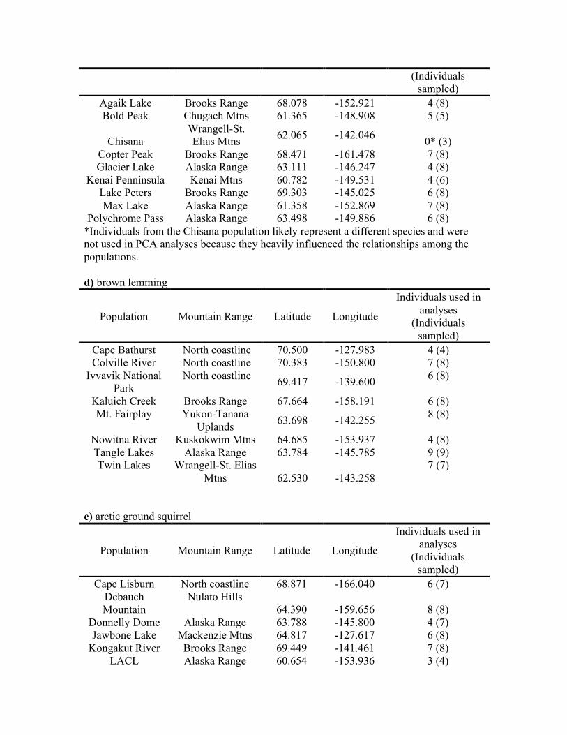
Table S1.2. Summary of genomic data collected in each individual. Shown are the raw count of reads from the Illumina run and the number of reads after processing for quality control (i.e., after excluding reads with low quality scores and ambiguous barcodes), as well as the number of reads analyzed with Stacks to identify homologous loci. Individuals excluded from analyses because of too few reads are marked with asterisks. Specimen IDs refer to University of Alaska Museum Mammalogy Collection catalog number (UAM) or sample IDs (Hik = David Hik lab, University of Alberta Edmonton). a) collared pika
Population Specimen
ID Raw read
count Post quality
control Analyzed
reads Percentage of raw reads used
Allie's Valley UAM 102431 2200193 2057166 1759078 80.0 Allie's Valley UAM 102422 1586907 1487171 1321899 83.3 Allie's Valley UAM 102435 1267564 1138753 1010043 79.7 Allie's Valley UAM 102438 1089077 1000485 882573 81.0 Allie's Valley UAM 102432 1195011 1033694 954753 79.9 Allie's Valley UAM 102423 510333 451607 350175 68.6 Allie's Valley UAM 102434 1179276 1114169 995286 84.4 Allie's Valley UAM 102424 1327323 1216267 1053178 79.3
Anchorage UAM 102564 774418 753014 523482 67.6 Anchorage UAM 102565 1126031 1065314 962098 85.4 Anchorage UAM 102566 3080176 2335737 2560219 83.1 Anchorage UAM 102567 1646939 1553367 1340924 81.4 Anchorage UAM 102568 1945449 1849269 1657894 85.2 Anchorage UAM 64363 420780 381384 278705 66.2
Crescent Creek UAM 58204 844108 786027 697267 82.6 Crescent Creek UAM 58205 1166926 1081539 982342 84.2 Crescent Creek UAM 58213 1876591 1755355 1637374 87.3 Crescent Creek UAM 58206 1984311 1742179 1674900 84.4 Crescent Creek UAM 58211 1605214 1410616 1277115 79.6 Crescent Creek UAM 58212 1771977 1520730 1446598 81.6 Crescent Creek UAM 58208 1627884 1418606 1305664 80.2 Denali Highway UAM 102482 1621668 1568650 1372480 84.6 Denali Highway UAM 102502 621042 564908 494274 79.6 Denali Highway UAM 102507 1157720 1107975 958350 82.8 Denali Highway UAM 102498 1072082 961926 838466 78.2 Denali Highway UAM 102497 1056373 1008968 860030 81.4 Denali Highway UAM 102562 1067428 969240 844903 79.2 Eagle Summit UAM 67030 2418283 2159229 2135761 88.3 Eagle Summit UAM 63938 858050 830613 709030 82.6 Eagle Summit UAM 63931 1147774 1090189 908065 79.1 Eagle Summit UAM 63935 1367964 1299827 1150204 84.1 Eagle Summit UAM 63932 1456907 1369052 1229103 84.4
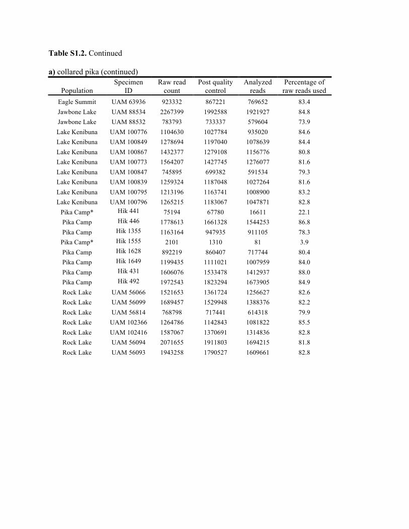
Table S1.2. Continued a) collared pika (continued)
Population Specimen
ID Raw read
count Post quality
control Analyzed
reads Percentage of raw reads used
Eagle Summit UAM 63936 923332 867221 769652 83.4 Jawbone Lake UAM 88534 2267399 1992588 1921927 84.8 Jawbone Lake UAM 88532 783793 733337 579604 73.9 Lake Kenibuna UAM 100776 1104630 1027784 935020 84.6 Lake Kenibuna UAM 100849 1278694 1197040 1078639 84.4 Lake Kenibuna UAM 100867 1432377 1279108 1156776 80.8 Lake Kenibuna UAM 100773 1564207 1427745 1276077 81.6 Lake Kenibuna UAM 100847 745895 699382 591534 79.3 Lake Kenibuna UAM 100839 1259324 1187048 1027264 81.6 Lake Kenibuna UAM 100795 1213196 1163741 1008900 83.2 Lake Kenibuna UAM 100796 1265215 1183067 1047871 82.8
Pika Camp* Hik 441 75194 67780 16611 22.1 Pika Camp Hik 446 1778613 1661328 1544253 86.8 Pika Camp Hik 1355 1163164 947935 911105 78.3
Pika Camp* Hik 1555 2101 1310 81 3.9 Pika Camp Hik 1628 892219 860407 717744 80.4 Pika Camp Hik 1649 1199435 1111021 1007959 84.0 Pika Camp Hik 431 1606076 1533478 1412937 88.0 Pika Camp Hik 492 1972543 1823294 1673905 84.9 Rock Lake UAM 56066 1521653 1361724 1256627 82.6 Rock Lake UAM 56099 1689457 1529948 1388376 82.2 Rock Lake UAM 56814 768798 717441 614318 79.9 Rock Lake UAM 102366 1264786 1142843 1081822 85.5 Rock Lake UAM 102416 1587067 1370691 1314836 82.8 Rock Lake UAM 56094 2071655 1911803 1694215 81.8 Rock Lake UAM 56093 1943258 1790527 1609661 82.8
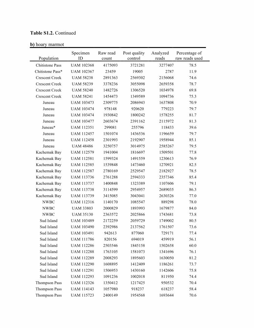
Table S1.2. Continued b) hoary marmot
Population Specimen
ID Raw read
count Post quality
control Analyzed
reads Percentage of raw reads used
Chitistone Pass UAM 102368 4175093 3721281 3277407 78.5 Chitistone Pass* UAM 102367 23459 19005 2787 11.9 Crescent Creek UAM 58238 2891363 2569302 2156068 74.6 Crescent Creek UAM 58239 3378236 3055098 2659358 78.7 Crescent Creek UAM 58240 1482726 1306520 1034978 69.8 Crescent Creek UAM 58241 1454473 1349589 1094736 75.3
Juneau UAM 103473 2309775 2086943 1637808 70.9 Juneau UAM 103474 978148 920620 779223 79.7 Juneau UAM 103474 1930842 1800242 1578255 81.7 Juneau UAM 103477 2603674 2391162 2115972 81.3
Juneau* UAM 112351 299081 255796 118433 39.6 Juneau UAM 112457 1501074 1436536 1196659 79.7 Juneau UAM 112458 2301993 2192907 1958944 85.1 Juneau UAM 48486 3250757 3014975 2585267 79.5
Kachemak Bay UAM 112579 1941004 1816697 1509501 77.8 Kachemak Bay UAM 112581 1599324 1491559 1230613 76.9 Kachemak Bay UAM 112585 1539848 1473460 1270921 82.5 Kachemak Bay UAM 112587 2780169 2529547 2182927 78.5 Kachemak Bay UAM 113736 2761288 2594333 2357346 85.4 Kachemak Bay UAM 113737 1400848 1323389 1107606 79.1 Kachemak Bay UAM 113738 3114599 2954957 2689035 86.3 Kachemak Bay UAM 113739 3415085 3043041 2630326 77.0
NWBC UAM 112316 1140170 1085547 889298 78.0 NWBC UAM 33803 2000829 1893993 1679877 84.0 NWBC UAM 35130 2363572 2025866 1743681 73.8
Sud Island UAM 103489 2172259 2059729 1749002 80.5 Sud Island UAM 103490 2392986 2137562 1761507 73.6 Sud Island UAM 103491 942613 877060 729171 77.4 Sud Island UAM 111786 820156 694019 459919 56.1 Sud Island UAM 112286 2503546 1845158 1502658 60.0 Sud Island UAM 112288 1763105 1581073 1341696 76.1 Sud Island UAM 112289 2008293 1895603 1630050 81.2 Sud Island UAM 112290 1608895 1412409 1186261 73.7 Sud Island UAM 112291 1506953 1430160 1142606 75.8 Sud Island UAM 112293 1091236 1002018 811950 74.4
Thompson Pass UAM 112326 1350412 1217425 950532 70.4 Thompson Pass UAM 114143 1057980 918237 618237 58.4 Thompson Pass UAM 115723 2400149 1954568 1693644 70.6
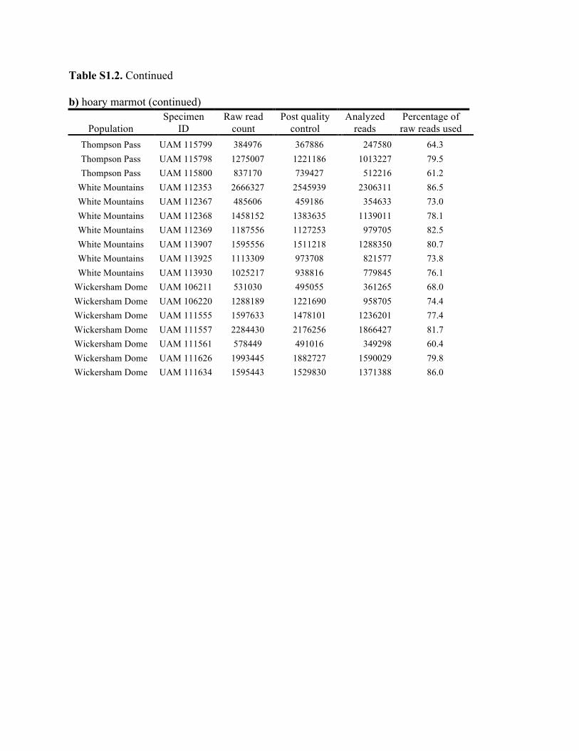
Table S1.2. Continued b) hoary marmot (continued)
Population Specimen
ID Raw read
count Post quality
control Analyzed
reads Percentage of raw reads used
Thompson Pass UAM 115799 384976 367886 247580 64.3 Thompson Pass UAM 115798 1275007 1221186 1013227 79.5 Thompson Pass UAM 115800 837170 739427 512216 61.2
White Mountains UAM 112353 2666327 2545939 2306311 86.5 White Mountains UAM 112367 485606 459186 354633 73.0 White Mountains UAM 112368 1458152 1383635 1139011 78.1 White Mountains UAM 112369 1187556 1127253 979705 82.5 White Mountains UAM 113907 1595556 1511218 1288350 80.7 White Mountains UAM 113925 1113309 973708 821577 73.8 White Mountains UAM 113930 1025217 938816 779845 76.1
Wickersham Dome UAM 106211 531030 495055 361265 68.0 Wickersham Dome UAM 106220 1288189 1221690 958705 74.4 Wickersham Dome UAM 111555 1597633 1478101 1236201 77.4 Wickersham Dome UAM 111557 2284430 2176256 1866427 81.7 Wickersham Dome UAM 111561 578449 491016 349298 60.4 Wickersham Dome UAM 111626 1993445 1882727 1590029 79.8 Wickersham Dome UAM 111634 1595443 1529830 1371388 86.0
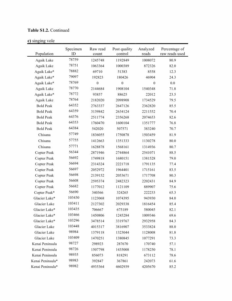
Table S1.2. Continued c) singing vole
Population Specimen
ID Raw read
count Post quality
control Analyzed
reads Percentage of raw reads used
Agaik Lake 78759 1245748 1192849 1008072 80.9 Agaik Lake 78751 1063364 1000389 872326 82.0
Agaik Lake* 78882 69710 51383 8558 12.3 Agaik Lake* 79097 192823 180426 46904 24.3 Agaik Lake* 78769 0 0 0 0.0 Agaik Lake 78770 2144684 1908104 1540348 71.8
Agaik Lake* 78772 93857 88625 22012 23.5 Agaik Lake 78764 2182020 2098908 1734529 79.5 Bold Peak 64352 2763337 2647126 2362820 85.5 Bold Peak 64359 3139842 2634124 2211552 70.4 Bold Peak 64376 2511774 2356268 2074653 82.6 Bold Peak 64353 1760470 1600104 1351777 76.8 Bold Peak 64384 542020 507571 383240 70.7 Chisana 57749 1836055 1750878 1503459 81.9 Chisana 57755 1412663 1351333 1130278 80.0 Chisana 57771 1628878 1568161 1314936 80.7
Copter Peak 56344 2871946 2744864 2541071 88.5 Copter Peak 56692 1749818 1680151 1381528 79.0 Copter Peak 56694 2314324 2221718 1791135 77.4 Copter Peak 56697 2052972 1964401 1715161 83.5 Copter Peak 56698 2139152 2053671 1717708 80.3 Copter Peak 56608 2595374 2482323 2202431 84.9 Copter Peak 56682 1177012 1121109 889907 75.6
Copter Peak* 56690 340366 324265 222233 65.3 Glacier Lake* 103430 1123068 1074395 943930 84.0 Glacier Lake 103411 2127302 2029338 1816454 85.4
Glacier Lake* 103435 706667 675189 580045 82.1 Glacier Lake* 103466 1450806 1245284 1009346 69.6 Glacier Lake* 103296 3478514 3319767 2932958 84.3 Glacier Lake 103448 4015317 3816907 3533824 88.0 Glacier Lake 98984 1379118 1323044 1128008 81.8 Glacier Lake 103409 1470251 1380845 1077291 73.3
Kenai Peninsula 98727 298923 287670 170740 57.1 Kenai Peninsula 98726 1507798 1435008 1178250 78.1 Kenai Peninsula 98935 856073 818291 673112 78.6
Kenai Peninsula* 98983 392847 367861 242073 61.6 Kenai Peninsula* 98982 4935364 4602939 4205670 85.2
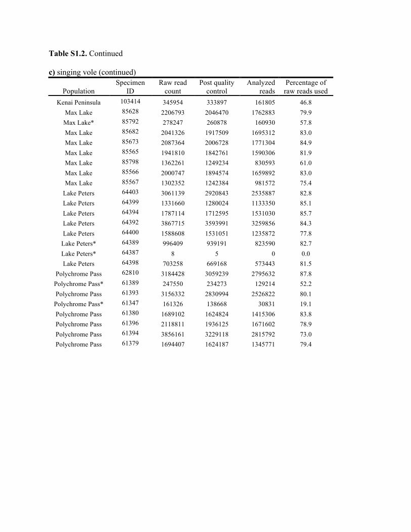
Table S1.2. Continued c) singing vole (continued)
Population Specimen
ID Raw read
count Post quality
control Analyzed
reads Percentage of raw reads used
Kenai Peninsula 103414 345954 333897 161805 46.8 Max Lake 85628 2206793 2046470 1762883 79.9
Max Lake* 85792 278247 260878 160930 57.8 Max Lake 85682 2041326 1917509 1695312 83.0 Max Lake 85673 2087364 2006728 1771304 84.9 Max Lake 85565 1941810 1842761 1590306 81.9 Max Lake 85798 1362261 1249234 830593 61.0 Max Lake 85566 2000747 1894574 1659892 83.0 Max Lake 85567 1302352 1242384 981572 75.4
Lake Peters 64403 3061139 2920843 2535887 82.8 Lake Peters 64399 1331660 1280024 1133350 85.1 Lake Peters 64394 1787114 1712595 1531030 85.7 Lake Peters 64392 3867715 3593991 3259856 84.3 Lake Peters 64400 1588608 1531051 1235872 77.8
Lake Peters* 64389 996409 939191 823590 82.7 Lake Peters* 64387 8 5 0 0.0 Lake Peters 64398 703258 669168 573443 81.5
Polychrome Pass 62810 3184428 3059239 2795632 87.8 Polychrome Pass* 61389 247550 234273 129214 52.2 Polychrome Pass 61393 3156332 2830994 2526822 80.1
Polychrome Pass* 61347 161326 138668 30831 19.1 Polychrome Pass 61380 1689102 1624824 1415306 83.8 Polychrome Pass 61396 2118811 1936125 1671602 78.9 Polychrome Pass 61394 3856161 3229118 2815792 73.0 Polychrome Pass 61379 1694407 1624187 1345771 79.4
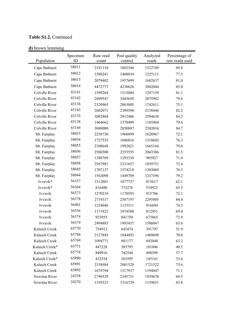
Table S1.2. Continued d) brown lemming
Population Specimen
ID Raw read
count Post quality
control Analyzed
reads Percentage of raw reads used
Cape Bathurst 58011 2181110 1802340 1522749 69.8 Cape Bathurst 58012 1580241 1468034 1225111 77.5 Cape Bathurst 58013 2078402 1957699 1682637 81.0 Cape Bathurst 58014 4472777 4230626 3802044 85.0 Colville River 43141 1599264 1515084 1297159 81.1 Colville River 43142 2609547 2443650 2075982 79.6 Colville River 43136 2320965 2063005 1742611 75.1 Colville River 43143 2602071 2389598 2138446 82.2 Colville River 43135 3082884 2912486 2594638 84.2 Colville River 43138 1464662 1370499 1165464 79.6 Colville River 43144 3048080 2850887 2582016 84.7 Mt. Fairplay 58053 2258730 1966099 1628967 72.1 Mt. Fairplay 58054 1727535 1606816 1318602 76.3 Mt. Fairplay 58055 2108648 1992821 1665164 79.0 Mt. Fairplay 58056 2506500 2355555 2043386 81.5 Mt. Fairplay 58057 1380789 1293338 985927 71.4 Mt. Fairplay 58058 2567981 2331657 1859751 72.4 Mt. Fairplay 58045 1707137 1574218 1303069 76.3 Mt. Fairplay 58044 1562098 1449789 1237396 79.2
Ivvavik* 56357 1312801 1077727 815617 62.1 Ivvavik* 56364 816480 733276 534923 65.5 Ivvavik 56373 1270218 1170593 915786 72.1 Ivvavik 56378 2719317 2587197 2295805 84.4 Ivvavik 56401 1234046 1133511 916694 74.3 Ivvavik 56356 1171825 1074588 812951 69.4 Ivvavik 56374 923955 841750 673865 72.9 Ivvavik 56379 2494885 1993457 1586047 63.6
Kaluich Creek 65770 754912 643474 391797 51.9 Kaluich Creek 65746 2127845 1844893 1489698 70.0 Kaluich Creek 65769 1094771 981177 692040 63.2
Kaluich Creek* 65771 447228 385795 181046 40.5 Kaluich Creek 65776 849916 742544 490398 57.7
Kaluich Creek* 65890 432554 363595 145141 33.6 Kaluich Creek 65891 2338984 2081529 1721522 73.6 Kaluich Creek 65892 1679794 1517937 1194847 71.1 Nowitna River 24338 2790529 2345731 1939670 69.5 Nowitna River 24270 1359323 1316729 1139651 83.8
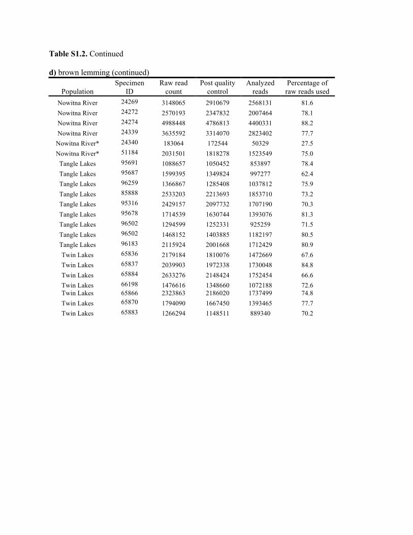
Table S1.2. Continued d) brown lemming (continued)
Population Specimen
ID Raw read
count Post quality
control Analyzed
reads Percentage of raw reads used
Nowitna River 24269 3148065 2910679 2568131 81.6 Nowitna River 24272 2570193 2347832 2007464 78.1 Nowitna River 24274 4988448 4786813 4400331 88.2 Nowitna River 24339 3635592 3314070 2823402 77.7
Nowitna River* 24340 183064 172544 50329 27.5 Nowitna River* 51184 2031501 1818278 1523549 75.0
Tangle Lakes 95691 1088657 1050452 853897 78.4 Tangle Lakes 95687 1599395 1349824 997277 62.4 Tangle Lakes 96259 1366867 1285408 1037812 75.9 Tangle Lakes 85888 2533203 2213693 1853710 73.2 Tangle Lakes 95316 2429157 2097732 1707190 70.3 Tangle Lakes 95678 1714539 1630744 1393076 81.3 Tangle Lakes 96502 1294599 1252331 925259 71.5 Tangle Lakes 96502 1468152 1403885 1182197 80.5 Tangle Lakes 96183 2115924 2001668 1712429 80.9 Twin Lakes 65836 2179184 1810076 1472669 67.6 Twin Lakes 65837 2039903 1972338 1730048 84.8 Twin Lakes 65884 2633276 2148424 1752454 66.6 Twin Lakes 66198 1476616 1348660 1072188 72.6 Twin Lakes 65866 2323863 2186020 1737499 74.8 Twin Lakes 65870 1794090 1667450 1393465 77.7 Twin Lakes 65883 1266294 1148511 889340 70.2
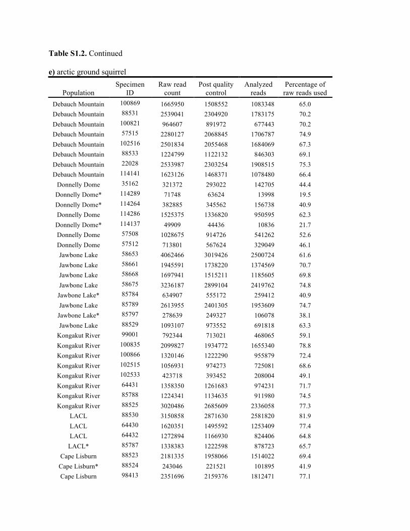
Table S1.2. Continued e) arctic ground squirrel
Population Specimen
ID Raw read
count Post quality
control Analyzed
reads Percentage of raw reads used
Debauch Mountain 100869 1665950 1508552 1083348 65.0 Debauch Mountain 88531 2539041 2304920 1783175 70.2 Debauch Mountain 100821 964607 891972 677443 70.2 Debauch Mountain 57515 2280127 2068845 1706787 74.9 Debauch Mountain 102516 2501834 2055468 1684069 67.3 Debauch Mountain 88533 1224799 1122132 846303 69.1 Debauch Mountain 22028 2533987 2303254 1908515 75.3 Debauch Mountain 114141 1623126 1468371 1078480 66.4
Donnelly Dome 35162 321372 293022 142705 44.4 Donnelly Dome* 114289 71748 63624 13998 19.5 Donnelly Dome* 114264 382885 345562 156738 40.9 Donnelly Dome 114286 1525375 1336820 950595 62.3
Donnelly Dome* 114137 49909 44436 10836 21.7 Donnelly Dome 57508 1028675 914726 541262 52.6 Donnelly Dome 57512 713801 567624 329049 46.1 Jawbone Lake 58653 4062466 3019426 2500724 61.6 Jawbone Lake 58661 1945591 1738220 1374569 70.7 Jawbone Lake 58668 1697941 1515211 1185605 69.8 Jawbone Lake 58675 3236187 2899104 2419762 74.8
Jawbone Lake* 85784 634907 555172 259412 40.9 Jawbone Lake 85789 2613955 2401305 1953609 74.7
Jawbone Lake* 85797 278639 249327 106078 38.1 Jawbone Lake 88529 1093107 973552 691818 63.3
Kongakut River 99001 792344 713021 468065 59.1 Kongakut River 100835 2099827 1934772 1655340 78.8 Kongakut River 100866 1320146 1222290 955879 72.4 Kongakut River 102515 1056931 974273 725081 68.6 Kongakut River 102533 423718 393452 208004 49.1 Kongakut River 64431 1358350 1261683 974231 71.7 Kongakut River 85788 1224341 1134635 911980 74.5 Kongakut River 88525 3020486 2685609 2336058 77.3
LACL 88530 3150858 2871630 2581820 81.9 LACL 64430 1620351 1495592 1253409 77.4 LACL 64432 1272894 1166930 824406 64.8
LACL* 85787 1338383 1222598 878723 65.7 Cape Lisburn 88523 2181335 1958066 1514022 69.4
Cape Lisburn* 88524 243046 221521 101895 41.9 Cape Lisburn 98413 2351696 2159376 1812471 77.1
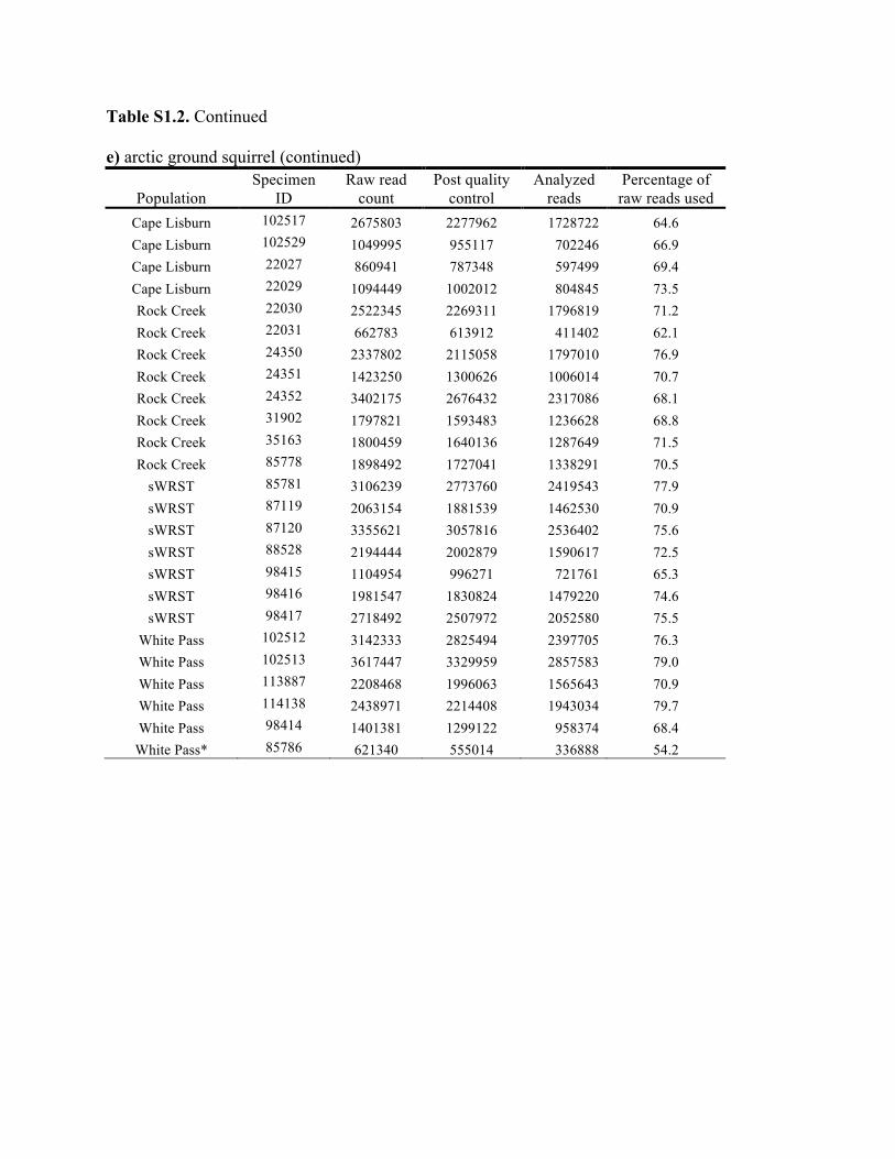
Table S1.2. Continued e) arctic ground squirrel (continued)
Population Specimen
ID Raw read
count Post quality
control Analyzed
reads Percentage of raw reads used
Cape Lisburn 102517 2675803 2277962 1728722 64.6 Cape Lisburn 102529 1049995 955117 702246 66.9 Cape Lisburn 22027 860941 787348 597499 69.4 Cape Lisburn 22029 1094449 1002012 804845 73.5 Rock Creek 22030 2522345 2269311 1796819 71.2 Rock Creek 22031 662783 613912 411402 62.1 Rock Creek 24350 2337802 2115058 1797010 76.9 Rock Creek 24351 1423250 1300626 1006014 70.7 Rock Creek 24352 3402175 2676432 2317086 68.1 Rock Creek 31902 1797821 1593483 1236628 68.8 Rock Creek 35163 1800459 1640136 1287649 71.5 Rock Creek 85778 1898492 1727041 1338291 70.5
sWRST 85781 3106239 2773760 2419543 77.9 sWRST 87119 2063154 1881539 1462530 70.9 sWRST 87120 3355621 3057816 2536402 75.6 sWRST 88528 2194444 2002879 1590617 72.5 sWRST 98415 1104954 996271 721761 65.3 sWRST 98416 1981547 1830824 1479220 74.6 sWRST 98417 2718492 2507972 2052580 75.5
White Pass 102512 3142333 2825494 2397705 76.3 White Pass 102513 3617447 3329959 2857583 79.0 White Pass 113887 2208468 1996063 1565643 70.9 White Pass 114138 2438971 2214408 1943034 79.7 White Pass 98414 1401381 1299122 958374 68.4
White Pass* 85786 621340 555014 336888 54.2
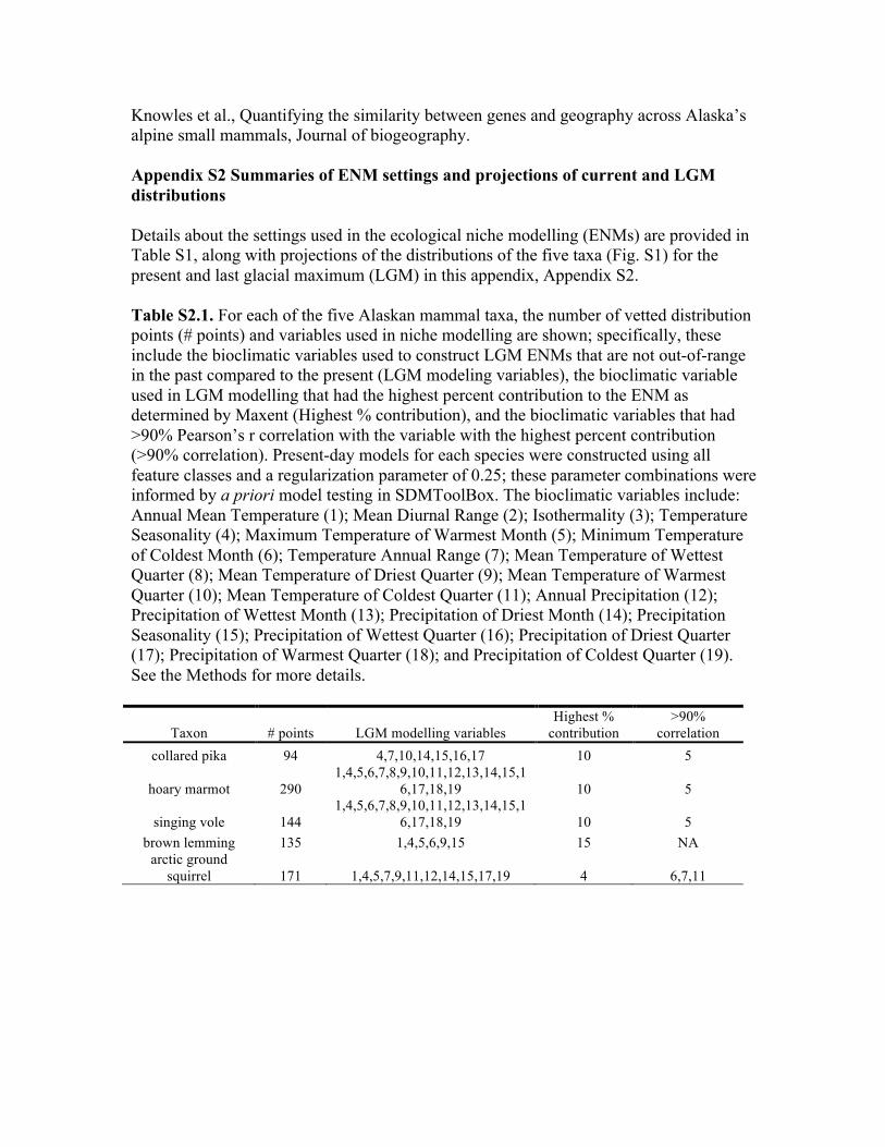
Knowles et al., Quantifying the similarity between genes and geography across Alaska’s alpine small mammals, Journal of biogeography. Appendix S2 Summaries of ENM settings and projections of current and LGM distributions Details about the settings used in the ecological niche modelling (ENMs) are provided in Table S1, along with projections of the distributions of the five taxa (Fig. S1) for the present and last glacial maximum (LGM) in this appendix, Appendix S2. Table S2.1. For each of the five Alaskan mammal taxa, the number of vetted distribution points (# points) and variables used in niche modelling are shown; specifically, these include the bioclimatic variables used to construct LGM ENMs that are not out-of-range in the past compared to the present (LGM modeling variables), the bioclimatic variable used in LGM modelling that had the highest percent contribution to the ENM as determined by Maxent (Highest % contribution), and the bioclimatic variables that had >90% Pearson’s r correlation with the variable with the highest percent contribution (>90% correlation). Present-day models for each species were constructed using all feature classes and a regularization parameter of 0.25; these parameter combinations were informed by a priori model testing in SDMToolBox. The bioclimatic variables include: Annual Mean Temperature (1); Mean Diurnal Range (2); Isothermality (3); Temperature Seasonality (4); Maximum Temperature of Warmest Month (5); Minimum Temperature of Coldest Month (6); Temperature Annual Range (7); Mean Temperature of Wettest Quarter (8); Mean Temperature of Driest Quarter (9); Mean Temperature of Warmest Quarter (10); Mean Temperature of Coldest Quarter (11); Annual Precipitation (12); Precipitation of Wettest Month (13); Precipitation of Driest Month (14); Precipitation Seasonality (15); Precipitation of Wettest Quarter (16); Precipitation of Driest Quarter (17); Precipitation of Warmest Quarter (18); and Precipitation of Coldest Quarter (19). See the Methods for more details.
Taxon # points LGM modelling variables Highest %
contribution >90%
correlation collared pika 94 4,7,10,14,15,16,17 10 5
hoary marmot 290 1,4,5,6,7,8,9,10,11,12,13,14,15,1
6,17,18,19 10 5
singing vole 144 1,4,5,6,7,8,9,10,11,12,13,14,15,1
6,17,18,19 10 5 brown lemming 135 1,4,5,6,9,15 15 NA
arctic ground squirrel 171 1,4,5,7,9,11,12,14,15,17,19 4 6,7,11
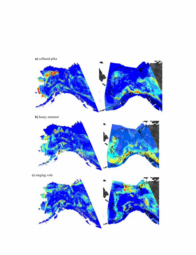
!!a) collared pika
b) hoary marmot
c) singing vole
Figure S1. Projections of the current (left) and LGM (right) distributions for each the five mammal taxa. Warmer colours indicate higher suitability of habitat, while cooler colours indicate unsuitable habitat!
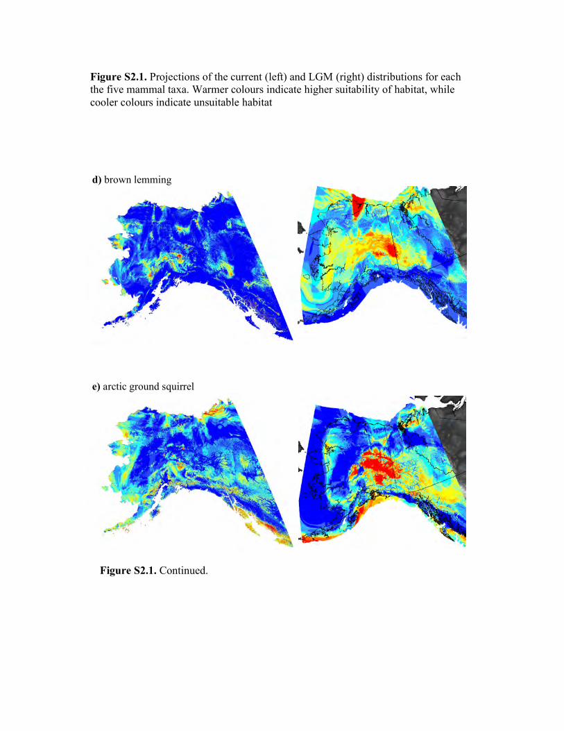
!!
!
!!
!!!!
d) brown lemming
e) arctic ground squirrel
Figure S1. Continued.!
Figure S2.1. Projections of the current (left) and LGM (right) distributions for each the five mammal taxa. Warmer colours indicate higher suitability of habitat, while cooler colours indicate unsuitable habitat
Figure S2.1. Continued.

Knowles et al., Quantifying the similarity between genes and geography across Alaska’s alpine small mammals, Journal of biogeography. Appendix S3 PC-maps of genetic variation and summaries of genetic variation Details about the patterns of genetic variation in each of the five taxa are given in this appendix, Appendix S3. This includes plots of genetic variation across individual from PC-analyses (Fig. S3.1), a comparison of taxa of the deviations from expectations based on the geographic sampling of individuals based on Procrustes analyses (Fig. S3.2), and sensitivity analyses of the strength of the association between genes and geography based on sequential exclusion of populations in Procrustes analyses (Table S3.1).
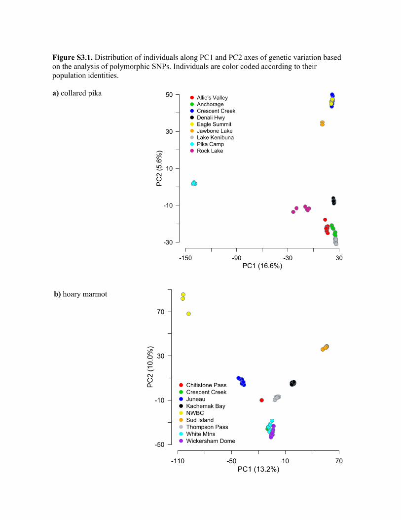
-110 -50 10 70
-50
-10
30
70
Chitistone PassCrescent CreekJuneauKachemak BayNWBCSud IslandThompson PassWhite MtnsWickersham Dome
PC1 (13.2%)
PC
2 (1
0.0%
)
b) hoary marmot
Figure S3.1. Distribution of individuals along PC1 and PC2 axes of genetic variation based on the analysis of polymorphic SNPs. Individuals are color coded according to their population identities.
a) collared pika
-150 -90 -30 30
-30
-10
10
30
50 Allie's ValleyAnchorageCrescent CreekDenali HwyEagle SummitJawbone LakeLake KenibunaPika CampRock Lake
PC1 (16.6%)
PC
2 (5
.6%
)
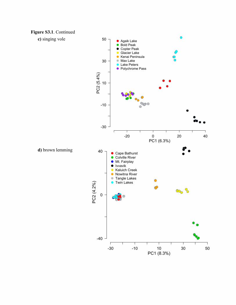
-20 0 20 40
-30
-10
10
30
50 Agaik LakeBold PeakCopter PeakGlacier LakeKenai PeninsulaMax LakeLake PetersPolychrome Pass
PC1 (6.3%)
PC
2 (5
.4%
)
c) singing vole Figure S3.1. Continued
d) brown lemming
-30 -10 10 30 50
-40
0
40 Cape BathurstColville RiverMt. FairplayIvvavikKaluich CreekNowitna RiverTangle LakesTwin Lakes
PC1 (8.3%)
PC
2 (4
.2%
)
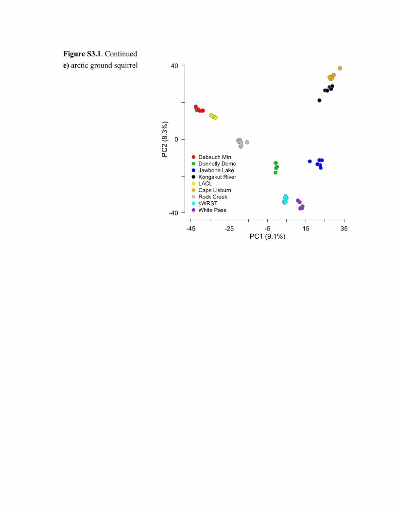
-45 -25 -5 15 35
-40
0
40
Debauch MtnDonnelly DomeJawbone LakeKongakut RiverLACLCape LisburnRock CreeksWRSTWhite Pass
PC1 (9.1%)
PC
2 (8
.3%
)
e) arctic ground squirrel Figure S3.1. Continued
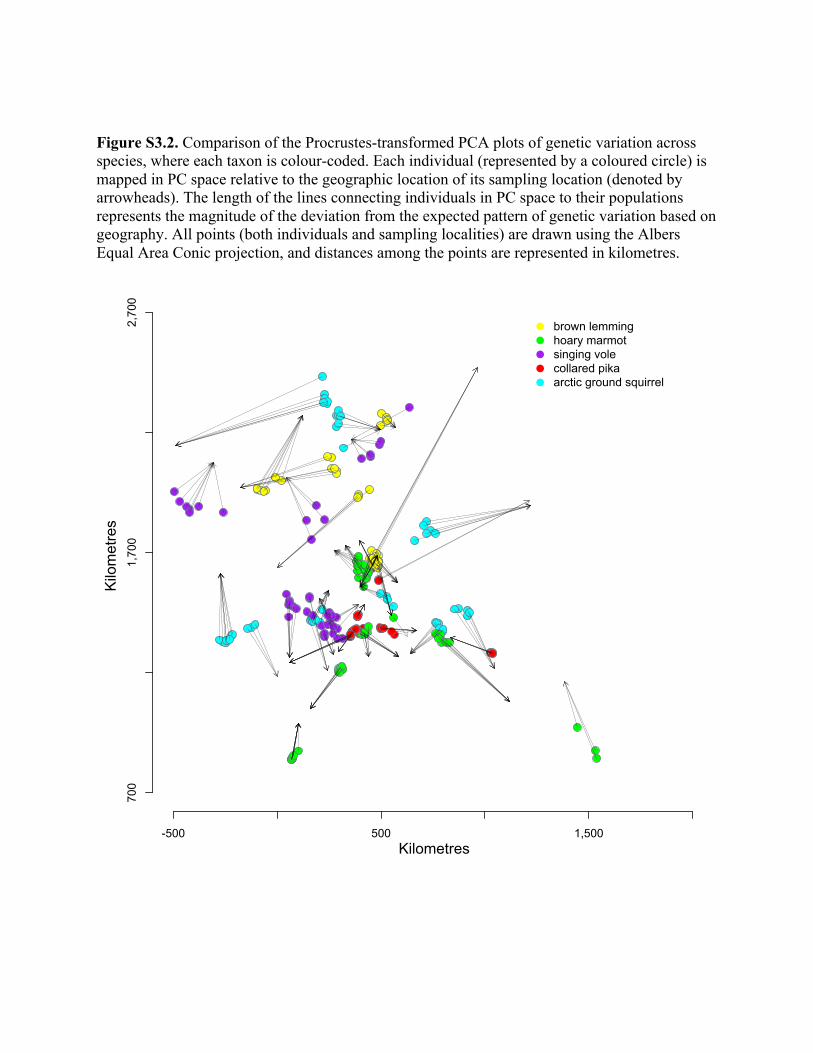
Figure S3.2. Comparison of the Procrustes-transformed PCA plots of genetic variation across species, where each taxon is colour-coded. Each individual (represented by a coloured circle) is mapped in PC space relative to the geographic location of its sampling location (denoted by arrowheads). The length of the lines connecting individuals in PC space to their populations represents the magnitude of the deviation from the expected pattern of genetic variation based on geography. All points (both individuals and sampling localities) are drawn using the Albers Equal Area Conic projection, and distances among the points are represented in kilometres.
-500 500 1,500
700
1,700
2,700
Kilometers
Kilometers
Brown lemmingHoary marmotSinging voleCollared pikaArctic ground squirrel
Brown Lemming Hoary Marmot Singing Vole Collared Pika Arctic Ground Squirrel
Kilometres
Kilo
met
res
brown lemming hoary marmot singing vole collared pika arctic ground squirrel
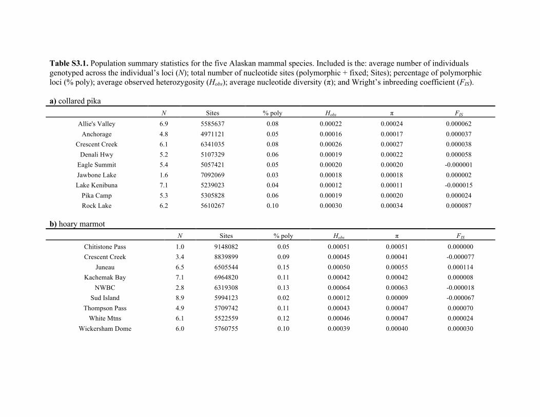
Table S3.1. Population summary statistics for the five Alaskan mammal species. Included is the: average number of individuals genotyped across the individual’s loci (N); total number of nucleotide sites (polymorphic + fixed; Sites); percentage of polymorphic loci (% poly); average observed heterozygosity (Hobs); average nucleotide diversity (π); and Wright’s inbreeding coefficient (FIS). a) collared pika
N Sites % poly Hobs π FIS
Allie's Valley 6.9 5585637 0.08 0.00022 0.00024 0.000062 Anchorage 4.8 4971121 0.05 0.00016 0.00017 0.000037
Crescent Creek 6.1 6341035 0.08 0.00026 0.00027 0.000038 Denali Hwy 5.2 5107329 0.06 0.00019 0.00022 0.000058
Eagle Summit 5.4 5057421 0.05 0.00020 0.00020 -0.000001 Jawbone Lake 1.6 7092069 0.03 0.00018 0.00018 0.000002 Lake Kenibuna 7.1 5239023 0.04 0.00012 0.00011 -0.000015
Pika Camp 5.3 5305828 0.06 0.00019 0.00020 0.000024 Rock Lake 6.2 5610267 0.10 0.00030 0.00034 0.000087
b) hoary marmot
N Sites % poly Hobs π FIS
Chitistone Pass 1.0 9148082 0.05 0.00051 0.00051 0.000000 Crescent Creek 3.4 8839899 0.09 0.00045 0.00041 -0.000077
Juneau 6.5 6505544 0.15 0.00050 0.00055 0.000114 Kachemak Bay 7.1 6964820 0.11 0.00042 0.00042 0.000008
NWBC 2.8 6319308 0.13 0.00064 0.00063 -0.000018 Sud Island 8.9 5994123 0.02 0.00012 0.00009 -0.000067
Thompson Pass 4.9 5709742 0.11 0.00043 0.00047 0.000070 White Mtns 6.1 5522559 0.12 0.00046 0.00047 0.000024
Wickersham Dome 6.0 5760755 0.10 0.00039 0.00040 0.000030
c) singing vole
N Sites % poly Hobs π FIS
Agaik Lake 3.0 2051233 0.18 0.00044 0.00087 0.000740 Bold Peak 4.1 1720098 0.13 0.00032 0.00050 0.000374 Chisana 2.0 1033820 0.16 0.00057 0.00089 0.000530
Copter Peak 5.8 1856071 0.21 0.00050 0.00076 0.000614 Glacier Lake 3.1 2320533 0.15 0.00043 0.00070 0.000475
Kenai Peninsula 2.8 1330770 0.06 0.00022 0.00032 0.000164 Max Lake 5.8 1714620 0.21 0.00049 0.00076 0.000613
Lake Peters 4.6 1944776 0.20 0.00051 0.00080 0.000605 Polychrome Pass 4.7 2264512 0.19 0.00046 0.00077 0.000642
d) brown lemming
N Sites % poly Hobs π FIS
Cape Bathurst 3.2 3131719 0.17 0.00054 0.00079 0.000438 Colville River 6.0 2492453 0.22 0.00061 0.00081 0.000467 Mt. Fairplay 6.5 2565557 0.28 0.00059 0.00091 0.000758
Ivvavik 4.8 2350735 0.17 0.00059 0.00069 0.000199 Kaluich Creek 4.4 2492971 0.25 0.00063 0.00097 0.000696 Nowitna River 3.1 3232862 0.24 0.00068 0.00108 0.000693 Tangle Lakes 7.5 1924798 0.25 0.00056 0.00081 0.000603 Twin Lakes 5.7 2095602 0.23 0.00053 0.00082 0.000654
e) arctic ground squirrel
N Sites % poly Hobs π FIS
Debauch Mtn 6.7 4759046 0.12 0.00037 0.00043 0.000128 Donnelly Dome 2.7 3101928 0.10 0.00038 0.00050 0.000196 Jawbone Lake 4.9 5469875 0.18 0.00057 0.00069 0.000238
Kongakut River 6.0 3966933 0.18 0.00052 0.00061 0.000221 LACL 2.7 4693453 0.10 0.00043 0.00048 0.000081
Cape Lisburn 4.9 4598436 0.12 0.00037 0.00047 0.000199 Rock Creek 6.6 4991411 0.19 0.00057 0.00065 0.000198
sWRST 6.1 5026303 0.13 0.00040 0.00050 0.000228 White Pass 4.4 5362339 0.13 0.00042 0.00054 0.000241
Table S3.2. Association statistics between genetic PCAs with all populations compared to genetic PCAs when single populations are excluded (i.e., t’), and between genetic PCAs and geography with the exclusion of individual populations (i.e., t”). The excluded populations are listed in the first row, and columns contain both the association statistics and the rotation in degrees (θ) that best aligns the 2 matrices. Positive values of θ indicate clockwise rotations and negative values indicate counterclockwise rotations. Note that θ-values marked with asterisks are not directly comparable with other values of θ within species because the PCAs that excluded those respective populations resulted in fundamentally different distributions of populations in PC space. a) collared pika, t0 = 0.71, θ = 73.1
Allie's Valley Anchorage
Crescent Creek Denali Hwy
Eagle Summit
Jawbone Lake
Lake Kenibuna Pika Camp Rock Lake
t' 0.99 1.00 0.99 1.00 0.99 1.00 0.99 0.89 1.00 θ -1.1 -1.6 3.6 -0.4 2.8 0.3 -2.8 -11.1 0.5
t" 0.76 0.68 0.70 0.71 0.70 0.79 0.69 0.77 0.71 θ 65.6 73.0 73.5 73.0 71.0 77.5 75.5 65.4 71.6
b) hoary marmot, t0 = 0.90, θ = -73.5
Chitistone Pass
Crescent Creek Juneau
Kachemak Bay NWBC Sud Island
Thompson Pass White Mtns
Wickersham Dome
t' 1.00 1.00 1.00 1.00 0.96 0.81 1.00 1.00 0.99 θ 0.4 -0.2 6.1 -4.4 28.6 46.9 -3.2 -1.7 -3.3
t" 0.90 0.88 0.95 0.92 0.96 0.84 0.92 0.86 0.83 θ -73.9 -73.3 -73.7 -69.9 51.4 -79.1* -70.5 -74.1 -73.4
c) singing vole, t0 = 0.89, θ = 30.2
Agaik Lake Bold Peak Copter Peak
Glacier Lake
Kenai Peninsula Max Lake Lake Peters
Polychrome Pass
t' 1.00 1.00 0.86 1.00 1.00 1.00 0.78 1.00 θ -0.6 2.6 44.6 -2.1 0.9 0.7 17.9 -2.2
t" 0.90 0.88 0.78 0.91 0.91 0.91 0.86 0.92 θ 27.6 33.0 -12.6* 26.0 31.1 29.5 49.2* 27.3
d) brown lemming, t0 = 0.60, θ = 33.2
Cape Bathurst
Colville River
Mt. Fairplay Ivvavik
Kaluich Creek
Nowitna River
Tangle Lakes Twin Lakes
t' 1.00 0.92 1.00 0.95 1.00 1.00 1.00 1.00 θ -0.1 21.7 0.0 13.2 1.4 0.0 0.7 0.0
t" 0.77 0.73 0.56 0.76 0.63 0.65 0.57 0.56 θ -24.7 -34.4 32.3 -47.0 23.1 31.6 37.8 35.8
e) arctic ground squirrel, t0 = 0.83, θ = 39.7
Debauch Mtn Donnelly
Dome Jawbone
Lake Kongakut
River LACL Cape Lisburn Rock Creek sWRST White Pass
t' 0.99 1.00 1.00 1.00 1.00 0.99 1.00 1.00 1.00 θ -58.9 3.5 36.6 -26.5 15.0 -24.3 14.9 -0.2 -11.0
t" 0.80 0.83 0.83 0.81 0.82 0.92 0.83 0.84 0.81 θ -25.9* 43.1 -2.8* -59.2 -26.9 -80.0 54.6 36.3 27.0
Recommended