Research Topics in Bioinformatics
Report title:
Different Representations of Multi-Domain Proteins;
Principal Component Analysis
Iwona Siuda
Student no.: 20097241

Iwona Siuda; RTiB Report
2
Content
1. Introduction .................................................................................................................................................. 3
2. Computer Simulations ................................................................................................................................. 4
2.1. Molecular Dynamics Simulations .......................................................................................................... 4
2.1.1. Force field ..................................................................................................................................... 4
2.1.2. Simulation setup ........................................................................................................................... 5
3. All Atom Simulations ................................................................................................................................... 6
3.1. AA System............................................................................................................................................. 6
3.2. AA Results............................................................................................................................................. 7
4. Simplified Methods....................................................................................................................................... 7
4.1. MARTINI Coarse Grained Approach.................................................................................................... 8
4.1.1. CG Basic Parametrization ................................................................................................................. 8
4.1.2. CG System ........................................................................................................................................ 9
4.1.3. CG Results ........................................................................................................................................ 9
4.2. ELNEDIN Approach ........................................................................................................................... 10
4.2.1. Elastic Network Parametrization ..................................................................................................... 11
4.2.2. ELNEDIN System ........................................................................................................................... 11
4.2.3. ELNEDIN Results ........................................................................................................................... 12
4.3. domELNEDIN Approach .................................................................................................................... 13
4.3.1. domELNEDIN System .................................................................................................................... 14
4.3.2. domELNEDIN Results .................................................................................................................... 14
5. Principal Component Analysis .................................................................................................................. 16
5.1. Mathematical Background ................................................................................................................... 16
5.1.1. Standard Deviation ..................................................................................................................... 16
5.1.2. Variance ...................................................................................................................................... 17
5.1.3. Covariance .................................................................................................................................. 18
5.1.4. Covariance Matrix ...................................................................................................................... 18
5.1.5. Eigenvalues and Eigenvectors .................................................................................................... 19
5.1.6. Generating New Vector and New Data ....................................................................................... 21
5.2. PCA of Trajectory using GROMACS ................................................................................................. 22
5.2.1. Generating Covariance Matrix .................................................................................................... 22
5.2.2. Analyzing Eigenvectors .............................................................................................................. 24
5.2.3. Graphical representation of principal components ...................................................................... 25
6. Conclusions ................................................................................................................................................. 28
References ............................................................................................................................................................ 29

Iwona Siuda; RTiB Report
3
1. Introduction
This report is divided into two parts. Part one contains brief descriptions of different
Molecular Dynamics (MD) methods, starting from well know all-atom (AA) approach, where
all atoms are well described, and interactions between them are modelled based on energy
potential functions. Next method described in this report is simplified method known as a
MARTINI Coarse Grained (CG) model [1-4], which is simplification of AA description at the
residue level, allowing longer simulations, but failing in reproducing secondary and tertiary
structure of protein. Third method is combination of MARTINI CG force field and additional
restraints put on top of initial protein structure [5]. This Elastic Network Model allows to
simulate proteins for longer time scale which is out of reach for AA simulations, but at the
same time keeping secondary and tertiary structure unchanged. However, there are some
biologically and chemically interesting phenomena that requires conformational changes. To
be able to observe those changes a new method is proposed, called domELNEDIN. In this
method the structural scaffold is put on to each domain separately, locking intra domains
movements, at the same time allowing inter domain movements. All methods are described
and compared.
The second part of the report describes Principal Component Analysis. It is also divided in
two. In part one all mathematical background is explained on simple example. The second
part is an evaluation of PCA on a trajectory obtained from AA simulation.
The report is closed with conclusions about all different MD description levels, as well as
about PCA.

Iwona Siuda; RTiB Report
4
2. Computer Simulations
Computer simulation provides us with a model which is generally simplified because of
deliberately neglecting factors with low impact on the test object (i.e., elimination of certain
external conditions). Thanks to the use of digital machines one can relatively accurately
mimic a real object or phenomenon. Computer simulation is a connection between theory and
experiment, and therefore often appears in the concept of a computer experiment. Simulation
methods allow assessment of the validity of the assumed model by comparing the results
obtained from simulation and experiment. They are also capable of verifying the theory by
comparing the theoretical and simulation results, referring to the same model. Often, after a
simulation, it appears that it is not only a confirmation of an existing theory, but it is also the
basis for new concepts.
2.1. Molecular Dynamics Simulations
Classical molecular dynamics simulations use Newton's equations of motion to
calculate trajectories of particles, starting from the defined configuration. For each particle in
the system, the total force acting on it is calculated from the interactions with other particles.
The acceleration, together with the prior position and velocity, determines what the new
position will be after a small time step.
2.1.1. Force field
A molecular dynamics simulation requires the definition of a potential function, or a
description of the terms by which the particles in the simulation will interact. Potentials may
be defined at many levels of physical accuracy; those most commonly used in chemistry are
based on molecular mechanics and embody a classical treatment of particle-particle
interactions that can reproduce structural and conformational changes but usually cannot
reproduce chemical reactions. Thus, the force acting on an atom can be found as a negative
derivative of the potential energy:
(1)
where the potential energy V is computed from bonded and non-bonded interactions:
(2)
where rij = ri − rj , kb is the bond stretching constant, r0 is the equilibrium bond distance, kθ is
the bond angle constant, θ0 is the equilibrium bond angle, τ is the torsion angle, ϕ is the phase
angle, and Vn is the torsional barrier. The last two non-bonded terms in the potential are

Iwona Siuda; RTiB Report
5
Lennard-Jones potential and coulomb interaction, in which
is the van der Waals well depth, σ is the van der Waals
diameter, q is the charge of each atom, and ε is dielectric
constant. The stretching and bending energy equations are
based on Hooke’s law, and they estimate the energy
associated with vibration about the equilibrium bond length
and bond angle, respectively. The torsion energy is used to
correct the remaining energy terms and represents the amount
of energy that must be added to or subtracted from other
energy terms to make the total energy agree with experiment
or quantum mechanical calculation for a model dihedral
angle. The non-bonded energy represents the pair-wise sum of
the energies of all possible interacting non-bonded atoms i < j. The non-bonded energy
accounts for repulsion (1/r12
dependency), van der Waals attraction that occurs at short range
(1/r6 dependency), and the electrostatic contribution modelled using a Coulombic potential.
The electrostatic energy is a function of the charge on the non-bonded atoms, their interatomic
distance, and a molecular dielectric expression that accounts for the attenuation of
electrostatic interaction by the environment. These equations together with the parameters
required to describe the behaviour of different kinds of atoms (i.e. atom types, atomic
charges) and bonds, are called a force-field.
2.1.2. Simulation setup
Molecular dynamics simulations consist of three stages: First, the input data has to be
prepared. Second, the production simulation can be run and finally the results have to be
analyzed and be put in context.
Before starting a simulation pdb structures have to be obtained. These can be retrieved
from the Protein Databank (1). The PDB file contains a lot of information regarding the
protein, the experimental methods used, conditions, and the Cartesian coordinates. Sometimes
when structure is disordered, and there are residues with missing side chains, it is necessary to
rebuild the structure. Sometimes the structure contains non-standard residues or ligands, in
this case it is advisable to find suitable parameters in literature or determine them. As there
are many types of force fields (CHARMM, AMBER GROMOS, OPLS) transferring
parameters from one force field to another is forbidden, as they cause different interactions,
and may misrepresent the results of simulation.
First step is to construct the topology, which describes the system in terms of atom
types, charges, bonds. It is important that the topology matches with the structure, which
means that the structure needs to be converted too. This can be done by Gromacs [6]
pdb2gmx program (for other methods described in next chapters PERL (5) and FORTRAN
(5) scripts are used). This program is designed to build topologies for molecules consisting of
amino acids and other building blocks. Using it hydrogen atoms present in the file will be
rebuilt according to the description in the force field. As the conversion of the structure
involves the deletion and/or addition of hydrogen atoms and may cause strain to be
introduced, e.g. due to atoms positioned too close together, it is necessary to perform an
r
τ
rij i j
θ
Figure 1. Description of different
parameters used in potential
energy equations.
Iwona Siuda; RTiB Report
6
energy minimization (EM) on the structure. This is done by combining the structure and the
topology into a single description of the system, together with a number of control parameters
for the energy minimization stored in em.mdp mdrun (2) file using grompp (2) command.
During the energy minimization the program generates output files and prints information
regarding the system and other control parameters. One piece of information is about the
charge of the system. As the structure is now relaxed, it should be solvated and minimized. To
add solvent the editconf (2) command is used. In this step the dimension of simulation box is
set up, and the solvent model, which is more or less intimately linked to a force field, is
chosen. If the system has non-zero charge it is necessary to add counter ions, which will
neutralize the system. To do so, some of solvent molecules are replaced by ions. This can be
done in two ways, by putting precise number of ions or adding ions up to a certain
concentration. The program genion (2) can take care of both tasks. As in the EM case it
requires an input file containing both the structure and the topology. Now the whole
simulation system is defined, but as ions are added, they may cause overlapping atoms or
equal charges that are too close together, the EM step has to be repeated. After all
minimization the solvent should adapt to the protein. It is done by position restraints of the
proteins’ non-hydrogen atoms keeping them more or less fixed to the reference positions so
the solvent move freely around the protein. The control parameters for this step are stored in
pr.mdp file, and once more the input file is generated by grompp command and mdrun to run
the simulation. The last step is to start a production run. In the control parameter md.mdp file
the number of steps multiplied with the time step describes the length of the simulation. There
are many different parameters that can be set up to efficiently mimic real behavior by the
simulated system. The last step is to take the final structure and topology files resulting from
the preparation and combine them into a run input file using grompp, and then using mdrun
command to run the simulation.
3. All Atom Simulations
MD simulations where all atoms of the biomolecular system are represented (AA) are
well-established and deliver a generous amount of details and insights of simulated system.
However, the time scale is limited to hundreds of nanoseconds (to run the simulation in
reasonable time), and the accessible timescale is mainly limited by the fastest movements in
the system which dictates the time steps size.
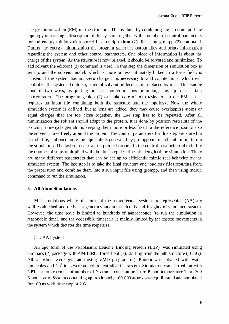
3.1. AA System
An apo form of the Periplasmic Leucine Binding Protein (LBP), was simulated using
Gromacs (2) package with AMBER03 force field (3), starting from the pdb structure (1USG).
All snapshots were generated using VMD program (4). Protein was solvated with water
molecules and Na+ ions were added to neutralize the system. Simulation was carried out with
NPT ensemble (constant number of N atoms, constant pressure P, and temperature T) at 300
K and 1 atm. System containing approximately 100 000 atoms was equilibrated and simulated
for 100 ns with time step of 2 fs.

Iwona Siuda; RTiB Report
7
3.2. AA Results
After analyzing trajectory it turns out that structure found its minimum energy
conformation and remained stable after first few ns of production run. The root mean square
deviation (RMSD) compared to the first frame of simulation, stays at the same level, around 3
Å (Fig. 2).
Figure 2. RMSD of LBP, AA simulation.
Analyzing snapshots from the simulation (Fig. 3), it can be observed that structure remains in
the same stable form confirming the behavior of the RMSD plot.
Figure 3. Snapshots from all-atom simulation at 0, 25, 50, 75, 100 ns.
The simulation is very stable and can be use as test bed, where structure and function of
protein and the effects of changing environment and thermodynamic settings can be tested
also the individual events in the protein function can be observed directly. In other words AA
MD are well-established and deliver a generous amount of information about studied system.
However, the time scale is limited to hundreds of nanoseconds, and the large conformational
changes are on the millisecond time scale, which is out of range for AA simulations.
4. Simplified Methods
When large structural rearrangements are involved, it is necessary to sample a time scale
in the micro- to millisecond range. The accessible timescale is mainly limited by the fastest
movements in the system which dictates the size of the time steps. However, as fast and slow
molecular dynamics are sufficiently independent, coarse grained descriptions of the system
can be applied. In a CG description fast vibrations are ignored, and a significant speedup is
gained compared to AA approaches. Recently, CG models have gained great popularity due to
their balance between accessible time scale and detail level.
0 20 40 60 80 100
0
1
2
3
4
5
6
Time [ns]
RM
SD [Å
]
Iwona Siuda; RTiB Report
8
4.1. MARTINI Coarse Grained Approach
MARTINI [2] is a CG force field which has become very popular due to its success in
parameterizing a large library of biologically relevant building blocks, and its also sufficiently
detailed description of system. Still, the CG models at this level fail to consistently reproduce
the secondary and tertiary structure of especially large and globular proteins, and different
ways of restraining the CG model to reproduce the correct structural scaffold have been
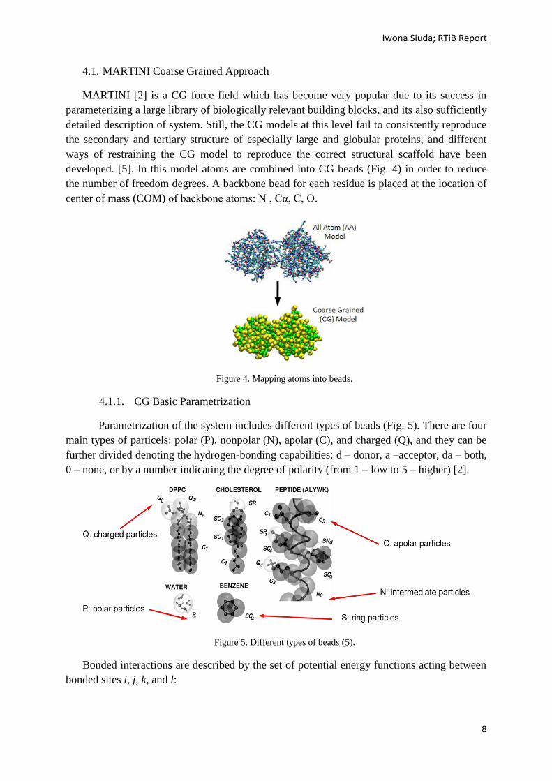
developed. [5]. In this model atoms are combined into CG beads (Fig. 4) in order to reduce
the number of freedom degrees. A backbone bead for each residue is placed at the location of
center of mass (COM) of backbone atoms: N , Cα, C, O.
Figure 4. Mapping atoms into beads.
4.1.1. CG Basic Parametrization
Parametrization of the system includes different types of beads (Fig. 5). There are four
main types of particels: polar (P), nonpolar (N), apolar (C), and charged (Q), and they can be
further divided denoting the hydrogen-bonding capabilities: d – donor, a –acceptor, da – both,
0 – none, or by a number indicating the degree of polarity (from 1 – low to 5 – higher) [2].
Figure 5. Different types of beads (5).
Bonded interactions are described by the set of potential energy functions acting between
bonded sites i, j, k, and l:

Iwona Siuda; RTiB Report
9
(3)
(4)
(5)
(6)
where r0 is equilibrium distance, υ0 angle, dihedral angles ψ0 and ψi0. The force constant k
includes flexibility of the molecule at CG level mimicking the collective motions at AA level.
Bonded potential Vbonds represents chemically bonded sites, angle potential Vangles chain
stiffness, and improper dihedral angle potential Vimpropers is used to prevent out-of-plane
distortions of planar groups. Proper dihedrals Vdihedrals are used to impose secondary structure
of the peptide backbone [2].
The non-bonded interactions between pairs of particle i and j at distance rij are
modeled using Lennard Jones potential:
(7)
where εij depends on interacting particle types i.e. for interactions between strongly polar
groups εij= 5.6 kJ/mol, but for groups mimicking the hydrophobic effect εij= 2.0 kJ/mol. The
effective size of particles is governed by LJ parameter σ, which for normal types of particle is
σ= 0.47 nm but for model ring-ring interactions is σ= 0.43 nm [2]. For charged groups
interactions between Q type beads are described via a Coulombic energy function, with a
relative dielectric constant εrel=15:
(8)
Non-bonded interactions between nearest neighbors are excluded [2].
4.1.2. CG System
The structure in minimum energy conformation from AA simulation was used to build
the CG system. After conversion of atoms into beads, equilibration procedure was carried out.
Protein was solvated with water molecules and counter Na+ ions were added. System was
simulated for 25 ns which corresponds to 100 ns of AA simulation [2] with a 25 fs time step
using NPT ensemble at 300K and 1atm. System contained approximately 9 500 beads. The
MARTINI-2.1 force field (4) was used.
4.1.3. CG Results
The MARTINI CG model without elastic network on top is not expected to be able to
maintain the overall structure of protein. Snapshots shows that structure is collapsing (Fig. 6),
and the RMSD (Fig. 7) is higher than in case of AA simulation.

Iwona Siuda; RTiB Report
10
Figure 6. Snapshots from CG simulation at 0, 25, 50, 75, 100 ns.
Figure 7. RMSD of LBP – AA simulation in red, CG simulation in blue.
The structural changes in the two models (AA and CG) are very different with RMSD ending
value 7.1 nm between the structures at 100 ns. When we compare RMSD per residue from
both simulations (Fig. 8) it appears that the CG model is too flexible compared with the AA
model.
Figure 6. RMSF per residue of LBP – AA simulation in red, CG simulation in blue.
The CG models at this level fail to consistently reproduce the secondary and tertiary structure
of presented protein. For modeling protein structure within this model, the secondary structure
needs to be stabilized by simple harmonic restraints on the backbone beads and is thereby not
allowed to change during a simulation. This approach is known as the ELNEDIN method [5].
4.2. ELNEDIN Approach
In ELNEDIN (Elastic Network in Dynamics) [5] model we put an elastic network on top
of a MARTINI model (Fig. 9) to restrain secondary and tertiary structure of protein.
0 20 40 60 80 100
0
1
2
3
4
5
6
7
8
Time [ns]
RM
DS
[Å]
0 100 200 300
0
1
2
3
4
5
6
7
Residue number
RM
SF_r
es [
Å]

Iwona Siuda; RTiB Report
11
Figure 9. Adding elastic network on top of CG model.
The basic idea remains the same as in CG model, with some exceptions. Firstly, the backbone
beads of residues are now placed at the location of Cα, and not in the COM like in simple CG.
Figure 9. Structural mapping and bond connectivity of residues Phe, Tyr, His and Trp. (supplement data to [5]).
Secondly, there is difference in maintaining the ring structure in residues. For both the Phe
and the Tyr the extra bond is used to maintain the ring structure, and in case of His and Trp
the asymmetry in rings is considered (Fig 10).
4.2.1. Elastic Network Parametrization
ELNEDIN is based on MARTINI approach and uses its force field for simulation. The
additional parameterization that has to be done concerns structural scaffold. There are two
main parameters that have to be set up before simulation, during the conversion from AA to
CG-ENM model. Those are: the cutoff distance between point of masses Rc [nm], which
describes the range of points that can be connected with additional elastic bond, and the
spring force constant Kspring [kJ·mol-1
·nm-2
], which describes stiffness of the elastic bond. The
range of those parameters is free, but the default that seems to work the best in most cases is
Rc = 0.9 nm and Kspring = 500 kJ·mol-1
·nm-2
[5]. For low Rc and Kspring the protein is more
flexible than for higher values of those parameters.
4.2.2. ELNEDIN System
Structure in minimum energy conformation from AA simulation was used to build
CG-ENM system. During conversion of atoms into beads different parameterization for
Coarse Grained (CG) Model
ELNEDIN Model

Iwona Siuda; RTiB Report
12
structural scaffold was used. The parameters were varied systematically with Rc [nm] ∈ {0.8,
0.9, 1.0} and Kspring [kJ·mol-1
·nm-2
] ∈ {50, 500, 5000}, then the equilibration procedure was
carried out. Protein was solvated with water molecules and counter Na+ ions were added.
System was simulated for 25 ns which corresponds to 100 ns of AA simulation [4] with a 10
fs time step using NPT ensemble at 300K and 1atm. System contained approximately 9 500
beads. The MARTINI-2.1 force field (1) was used.
4.2.3. ELNEDIN Results
The model is constructed to represent a structural scaffold around the initial structure.
The collapse is therefore not seen in this case (Fig 11.) and RMSD remains stable at the same
level as for the AA simulation (Fig 12.).
Figure 11. Snapshots from CG-ENM simulation at 0, 25, 50, 75, 100 ns.
Figure 12. RMSD per residue of LBP – AA simulation in red, CG-ENM simulation in green.
0 20 40 60 80 100
0
1
2
3
4
5
6
Time [ns]
RM
DS
[A]

Iwona Siuda; RTiB Report
13
Figure 13. RMSF per residue of LBP – AA simulation in red, CG-ENM simulation in black.
For all different scaffold settings it seems that proposed values [5] are in the best agreement
with AA in reproducing its flexibility (Fig. 13). However, as the structural scaffold is put on
top of the initial conformation of simulated protein, structural changes can’t be observed. In
this case different approach is needed.
4.3. domELNEDIN Approach
This model is based on ELNEDIN method with difference in the way of combining ENM
with MARTINI CG model. The structural scaffold is put on each domain of the protein
separately, meaning that there are no elastic bonds connecting atoms from different protein
domains.
Figure 14. Adding elastic network on each domain separately of CG model.
Coarse Grained (CG) Model
domELNEDIN Model

Iwona Siuda; RTiB Report
14
It is possible to lock inter domains movements, as the RMSD between the same domains in
two different LBP conformations (open and closed form) are much smaller than overall
RMSD between those conformations. This approach is called domELNEDIN and allows
protein to change conformations thanks to free domain movements with respect to each other.
4.3.1. domELNEDIN System
All steps are exactly the same as in simple ELNEDIN model. Structure in minimum
energy conformation from AA simulation was used to build CG-ENM system. During
conversion of atoms into beads different parametrization for structural scaffold was used
varying systematically with Rc [nm] ∈ {0.8, 0.9, 1.0} and Kspring [kJ·mol-1
·nm-2
] ∈ {50, 500,
5000}, although the ENM was put on each domain separately. The equilibrated procedure was
carried out including protein solvation with water molecules and addition of counter Na+ ions.
System was simulated for 25 ns which corresponds to 100 ns of AA simulation [4] with a 10
fs time step using NPT ensemble at 300K and 1atm. System contained approximately 9 500
beads. The MARTINI-2.1 force field (1) was used.
4.3.2. domELNEDIN Results
The model is constructed to allow free domain movements while maintaining the internal
domain structures. Analyzing snapshots can be observed that second domain changed its
position with respect to the first one at 100 ns (Fig. 14).
Figure 14. Snapshots from domELNEDIN simulation at 0, 25, 50, 75, 100 ns.
For all different scaffold settings it seems that proposed values for ELNEDIN model [5] are
also the best for domELNEDIN in reproducing AA flexibility (Fig. 15).

Iwona Siuda; RTiB Report
15
Figure 15. RMSF per residue of LBP – AA simulation in red, domENEDIN simulation in black.
This model is as limited as the original ELNEDIN model with respect to reproducing the
observed AA flexibility within the domains. However, it is more flexible than the ELNEDIN
model, due to the non-existing interdomain restraints (Fig. 16). The structure at 100 ns from
the ELNEDIN and domELNEDIN simulations differ with RMSD of 2.6 Å.
Figure 16. RMSF per residue of LBP – ELNEDIN in green, domELNEDIN in black.
0 100 200 300
0
0,5
1
1,5
2
2,5
Residue number
RM
SF_r
es [
Å]

Iwona Siuda; RTiB Report
16
5. Principal Component Analysis
When measuring only two variables, and then analyzing them using different conditions it
is easy to plot this data and to visually assess the correlation between these two factors.
However, when number of factors increase to thousands, it becomes impossible to make
visual inspection of the relationship between those factors or conditions describing them . One
way to make sense of this data is to use Principal Component Analysis (PCA), which is a
common statistical technique for finding and identifying patterns in data of high dimension,
and expressing it in such a way as to highlight their similarities and differences. The main
advantage of PCA is that once you have found these patterns in your dataset you can
compress the data, i.e. by reducing the number of dimensions, without much loss of
information.
5.1. Mathematical Background
To use PCA it is necessary to understand mathematics on which this method is based. The
background knowledge presented in this chapter covers standard deviation, covariance,
eigenvectors and eigenvalues. For this purposes 2-dimensional made-up data set is used.
5.1.1. Standard Deviation
Assume there are two example sets describing the same event, set1 and set2:
set1 = (36 40 45 44 26 33 38 32 36 55 23 48) (9)
set2 = (8 35 20 24 15 29 28 25 20 40 9 35). (10)
There are number of things that can be calculated from those datasets, such as the mean value:
(11)
where Xi refer to an individual number in this data set, and n is a number of elements in the X
set. To find mean value all numbers in data set are summed up and then divided by the total
number of individuals. The mean describes a value for a middle point, for example for set1
the middle point is 38, and for set2 it is 24. We can use mean value to measure how spread the
data is, calculating the average distance from the mean of the data set to a point. This is
known as the Standard Deviation (SD). For computing SD of a sample s, the squares of the
distance from each data point to the mean of the set are computed, summed, divided by (n –
1), and then the positive square root is taken:
(12)

Iwona Siuda; RTiB Report
17
set1
Xi
36 -2 4
40 2 4
45 7 49
44 6 36
26 -12 144
33 -5 25
38 0 0
32 -6 36
36 -2 4
55 17 289
23 -15 225
48 10 100
s 9.13
set2
Xi
8 -16 256
35 11 121
20 -4 16
24 0 0
15 -9 81
29 5 25
28 4 16
25 1 1
20 -4 16
40 16 256
9 -15 225
35 11 121
s 10.15
Table 1. Calculation of standard deviation.
For two data sets above, it is shown (Tab.1 and Fig. 17) that the second set has a much larger
standard deviation (10.15) than the first one (9.13) due to the fact that the data is much more
spread out from the mean value.
Figure 17. Plot of original data from set1 and set2.
5.1.2. Variance
Variance is another measure of the spread of data in a data set, and for sample of data
is defined as:
(13)
0
10
20
30
40
50
60
0 10 20 30 40 50 60
set2
set1

Iwona Siuda; RTiB Report
18
SD s is the square root of the variance s2. For set1 variance s
2 = 83.27 and for set2 s
2 = 103.09,
the theory [7] states that first principal component has a larger variance than any of the others,
thus values from set2 will be based to build the first PC.
5.1.3. Covariance
Standard deviation and variance only operate on 1 dimension, so that one can only
calculate the standard deviation for each dimension of the data set independently of the other
dimensions. However, it is useful to have a similar measure to find out how much the
dimensions vary from the mean with respect to each other. Covariance is such a measure
between 2 dimensions, so two data sets X and Y each containing n values of variables can
define covariance as:
(14)
The most important information from this measurement is a sign of the result. If the value is
positive, than it indicates that both dimensions (X and Y) increase together, meaning that if the
values from data set X increase so do the values from set Y. If the value is negative, than
dimensions behave in opposite way, if one increases, the other has to decrease. Beside
negative and positive value, covariance between 2 dimensions can be zero, meaning that they
are independent of each other. For sets set1 and set2 covariance is cov(X,Y) = meaning
that they are positively correlated.
5.1.4. Covariance Matrix
If there are more than two data sets, the covariance matrix C can be set as:
(15)
where is a square matrix with n rows and n columns, and Dimi and Dimj are the ith and
jth dimensions, respectively. In simple way each entry in the matrix is the result of calculating
the covariance between two separate dimensions, and for described above example it is 2
dimensional.
(16)
Down the main diagonal, the covariance value is between one of the dimensions and itself
meaning that it is nothing else than the variances for that dimension. The other point is that
the matrix is symmetrical about the main diagonal, as .

Iwona Siuda; RTiB Report
19
5.1.5. Eigenvalues and Eigenvectors
Many application problems involve applying a linear transformation repeatedly to a given
vector. The key to solving these problems is to choose a coordinate system or basis for which
it will be simpler to do calculations involving the operator. If for this equation:
(17)
where A is n x n square matrix, exist nonzero solution x then λ is said to be an eigenvalue of
A, and x is said to be an eigenvector belonging to λ. The eigenvectors can only be found for
square matrices, but not every square matrix has eigenvectors. Usually for n x n there are n
linearly independent eigenvectors. Another property of eigenvectors is that even if the vector
is scaled by some amount before multiplying it, it will still get the same multiple of it as a
result, as it is not changing its direction but it is getting longer. All the eigenvectors of a
matrix are orthogonal.
Since example covariance matrix is square, the eigenvectors and eigenvalues can be
calculated:
(17)
The characteristic equation is:
or (18-19)
Thus, the eigenvalues of C are λ1 = 32.53 and λ2 = 153.83. The sum of the firs k eigenvalues
divided by the sum of all the eigenvalues, represent the proportion of total variation explained
by the first k principal components [7]. In other words the first principal component explains
153.83/186.36 = 82.54% of the total variation, while second one only 32.53/186.36 = 17.46%,
those two PCs explains total motility in the example sets.
To find the eigenvectors belonging to λ1, the nullspace of C - 32.53I has to be
determined, I denotes diagonal matrix, and nullspace means the set of all vectors x for which
Ax = 0.
(20)
Solving (C - 32.53 I)x = 0, we get
1.18, -1)T (21)
Thus, any nonzero multiple of 1.18, -1)T is an eigenvector belonging to λ1. Similarly, to find
the eigenvectors for λ2, (C - 153.83 I)x = 0 has to be solved.
(22)

Iwona Siuda; RTiB Report
20
In this case any nonzero multiple of -0.84801, -1)T is an eigenvector belonging to λ2. Another
important thing to know about eigenvectors is that they are scaled to have a length of 1 in
order to keep them standard. This is because, the length of a vector doesn’t affect whether it’s
an eigenvector or not, whereas the direction does. To scale eigenvectors the original vector
has to be divided by its length. The first eigenvector is then presented as:
(23)
and the second eigenvector:
(24)
Eigenvectors can be presented as:
(25)
It is important for PCA that these eigenvectors are both unit eigenvectors i.e. their lengths are
both 1.
Figure 18. A plot of the normalized data with the eigenvectors of the covariance matrix overlayed on top. First
eigenvector – dashed line. Second eigenvector – dotted line.
As expected from the covariance matrix, two variables do indeed increase together. They
appear as diagonal dotted and dashed lines on the plot. They are perpendicular to each other,
and they go through the middle of the points, like drawing a line of best fit. The eigenvector
mark as a dotted line is showing that these two data sets are related along that line. The
-30
-20
-10
0
10
20
30
-30 -10 10 30
Dev
iati
on f
rom
mea
n v
alue
set2
Deviation from mean value set1

Iwona Siuda; RTiB Report
21
second eigenvector gives the other, less important, pattern in the data, that all the points
follow the main line, but are off to the side of the main line by some amount. So, by this
process of taking the eigenvectors of the covariance matrix, lines that characterize the data
have been extracted. It turns out that the eigenvector with the highest eigenvalue is the
principal component of the data set. In general, once eigenvectors are found from the
covariance matrix, the next step is to order them by eigenvalue, highest to lowest.
5.1.6. Generating New Vector and New Data
A new vector is a name for a matrix of vectors, constructed by taking the eigenvectors that
one want to keep from the list of eigenvectors, and forming a matrix with these eigenvectors
in the columns. For the example sets it will look the same as eigenvector matrix:
(26)
. (27)
One may consider both eigenvectors or take only one that is more significant to describe the
data set:
. (28)
The last step is to take the transpose of NewVector so that the eigenvectors in the columns are
now in the rows, with most significant eigenvector at the top, and multiply it by the
DataAdjust which is a matrix containing values of deviation from mean for both set1 and set2,
also transposed.
(29)
Table.2 NewData derived from transformation with eigenvectors.
Data transformed with first eigenvector Data transformed with second eigenvector
13.49654 8.82288
-9.6831 -5.58905
-1.47661 7.92588
-3.8806 4.576128
14.62538 -3.33136
-0.57961 -7.04727
-3.05075 -2.58706
3.117908 -5.22289
4.344284 1.061688
-23.198 2.61744
21.14181 -1.73883
-14.8572 0.512454

Iwona Siuda; RTiB Report
22
1
Figure 19. Data transformed with 2 eigenvectors, presenting a new data points.
In Fig. 19. the data is presented using both eigenvectors for the transformation; this plot
presents the original data, rotated so that the eigenvectors are the axes, as there is no
information lost in this decomposition. PCA allows to express original data that was in term
of two axes (x,y) in terms of any two axes. If these axes are perpendicular, then the expression
is the most efficient. This was why it is important that eigenvectors are always perpendicular
to each other. When the new data set has reduced dimensionality, then it is only presented in
terms of the vectors that have left.
5.2. PCA of Trajectory using GROMACS
In structural bioinformatics PCA is applied to a set of molecular conformations. In this
chapter trajectory from AA simulation described in Chapter 3 is analyzed using Gromacs v.
4.0.7 package.
5.2.1. Generating Covariance Matrix
First the covariance matrix is constructed, using g_covar program, which computes the
covariance matrix of fluctuational motion from an MD trajectory x(t). g_covar removes
rotational and translational motion by least square fitting to a reference structure, allowing to
look at the internal motion only. Covariance matrix C of the atomic coordinates is a
symmetric 3N x 3N matrix described as:
1 In previous statement it was called second eigenvector, but as it gives the highest contribution to PCA (it is an
eigenvector corresponding to the highest eigenvalue) we will now referred to it as a first eigenvector.
-30
-20
-10
0
10
20
30
-30 -20 -10 0 10 20 30
Dat
a tr
ansf
orm
ed w
ith s
econd
eigen
vec
tor
Data transformed with first eigenvector1

Iwona Siuda; RTiB Report
23
(30)
where M is diagonal matrix containing the masses of the atoms (mass-weighted analysis) or
the unit matrix (non-mass weighted-analysis). The covariance matrix C can be diagonalized
with an orthonormal transformation matrix R:
(31)
R defines a transformation to a new coordinate system and the columns of R are the
eigenvectors (stored in eigenvec.trr file), also called principal modes. Using command
g_covar covariance matrix is generated for 345 Cα atoms:
g_covar -f traj.xtc -s ref_str.pdb -o eigenval.xvg -v eigenvec.trr –ascii covar.dat
Where flag –f means an input file with trajectory (traj.xtc – 400 frames), -s an input for
coordinate file with reference structure (ref_str.pdb). Flags –v means that eigenvectors are
written to a full precision trajectory file (eigenvec.trr), and –o means output for eigenvalues
(eigenval.xvg). Flag –ascii writes the whole covariance matrix to an ASCII file.
Figure 20. Covariance matrix computet for 345 Cα atoms.
Fig. 20. presents matrix showing coordinate covariances between Cα atoms. Red mean that
two atoms move together, so it is reasonable that on diagonal there is a red line. Blue means
that they move in opposite directions. The intensity of colors indicates the amplitude of the
fluctuations. From the covariance matrix it is possible to see that group of atoms move in a
correlated or anti-correlated manner. Knowing that first domain contains Cα with indexes 1 to
120 and 250 to 330, and second domain Cα with indexes 121 to 249 and 331 to 345, it is
observable that correlation between atoms in the same domains is higher (lighter areas in the
plot), meaning that they move in the same group of atoms. In case when atoms from first
0
50
100
150
200
250
300
0 50 100 150 200 250 300
Cα atom number
Cα
ato
m n
um
ber

Iwona Siuda; RTiB Report
24
domain are correlated with atoms from second domain the intensity of blue is much higher
meaning that both domains move opposite to each other.
Another important measurement from covariance matrix is a trace of it tr = 4.8122 nm2 and it
is a sum of the eigenvalues. As mentioned in (5.1.5) this sum can be used to describe total
motility. There are some rules for excluding principal component [1]. One of them says to
include just enough components to explain 90% of total motility. Second called Kaiser’s
criterion excludes those PC whose eigenvalues are less than average, i.e. less than one if a
correlation matrix has been used. In practice often compromise is used, thus Fig. 21. presents
the percentage and cumulative percentage of variance explained by first 100 from 1035
eigenvalues. It is shown that 50 first from 1035 eigenvalues can describe approximately 90%
of total variation it the system.
Figure 21. Percentage (black) and cumulative percentage (red) of variance for first 50 eigenvalues.
5.2.2. Analyzing Eigenvectors
Each amino acid in this example is represented by its Cα atom. As position of each
atom is described by 3 coordinates (x, y, z), the covariance matrix has the dimension of 3N x
3N, where N is the number of atoms (in this case N refers to number of amino acids in the
protein). So as matrix is 3 dimensional it has 3 x 345 = 1035 rows and columns and 1035
eigenvalues. For the 3N x 3N coordinate matrix there are 345 3-dimentional (x, y ,z)
eigenvectors computed for each of 400 frames. Below is presented fragment of eigenvec.trr
file, showing first 8 eigenvectors x for the first frame (counted from n-1):
eigenvec.trr frame 0:
natoms=345 step=0 time=0.0000000e+00 lambda=0
box (3x3):
box[ 0]={ 0.00000e+00, 0.00000e+00, 0.00000e+00}
box[ 1]={ 0.00000e+00, 0.00000e+00, 0.00000e+00}
box[ 2]={ 0.00000e+00, 0.00000e+00, 0.00000e+00}
x (345x3):
x[ 0]={ 1.18355e+00, 3.99314e-01, 3.27480e+00}
x[ 1]={ 1.07012e+00, 4.93567e-01, 2.95261e+00}
0 5 10 15 20 25 30 35 40 45 50
0
10
20
30
40
50
60
70
80
90
100
Eigenvalue index
Per
centa
ge
of
var
iance
expla
ined
by e
ach e
igen
val
ue
(%)

Iwona Siuda; RTiB Report
25
x[ 2]={ 1.11421e+00, 3.34410e-01, 2.61641e+00}
x[ 3]={ 1.23923e+00, 5.36954e-01, 2.32276e+00}
x[ 4]={ 1.10660e+00, 5.02108e-01, 1.96799e+00}
x[ 5]={ 1.17910e+00, 7.05479e-01, 1.65667e+00}
x[ 6]={ 9.10663e-01, 8.00125e-01, 1.40656e+00}
x[ 7]={ 1.02828e+00, 8.88123e-01, 1.05605e+00}
x[ 8]={ 8.29841e-01, 1.02164e+00, 7.61136e-01}
Plot below (Fig. 22) presents components of each of 8 first eigenvectors for 345 Cα atoms.
Figure 22. Components of first 8 eigenvectors; coordinate x in red, y in green, z in blue.
5.2.3. Graphical representation of principal components
The trajectory can be projected on eigenvectors to give the principal components pi(t):
(32)
The eigenvalue is the mean square fluctuation of principal component i. The first few PCs
often describe collective, global motions in the system. The trajectory can be filtered along
one (or more) PCs. For one PC this goes as follows:

Iwona Siuda; RTiB Report
26
(33)
The reduction in dimensions afforded by principal component analysis can be used
graphically. Thus if the first two components explain most of motility, then a plot showing the
distribution of the objects on these two dimensions will often give a fair indication of the
overall distribution of data.
Figure 23. Data projection on eigenvectors.
In Fig. 23 (starting from top left) data is plotted on the first two eigenvectors of the covariance
matrix, showing equally distribution, where each point corresponds to the one trajectory
frame. Second plot shows that the variance along the eigenvector 1 axis is greater than along
the eigenvector 8 axis, meaning that eigenvector 8 provides less information about protein
behavior. The last plot presents projection on eigenvectors 7 and 8 showing that their
contribution to total motility is much smaller than the one presented on firs plot, but
correlation between data is much bigger.
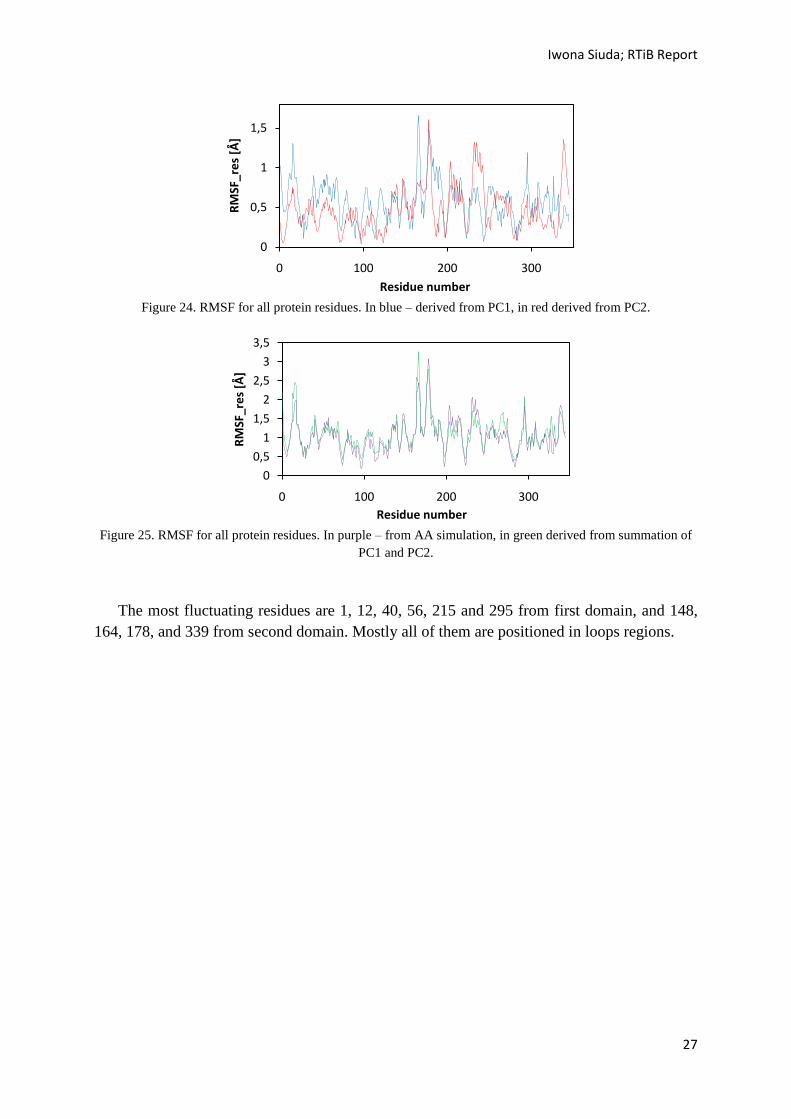
Because the covariance matrix is defined in terms of deviations from the trajectory-
averaged coordinates, based on eigenvectors the RMSF plot can be presented (Fig. 24). In
blue line are indicated fluctuations from the first PC, and in red line fluctuations from the
second principal component. When for each atom, fluctuations from both PCs are summed
and compared with the plot from Chapter 4 (Fig. 6: AA fluctuations) it is clear that there is
not much information that was lost, and only two firs PCs are sufficient do describe
fluctuations in protein (Fig. 25).
Iwona Siuda; RTiB Report
27
Figure 24. RMSF for all protein residues. In blue – derived from PC1, in red derived from PC2.
Figure 25. RMSF for all protein residues. In purple – from AA simulation, in green derived from summation of
PC1 and PC2.
The most fluctuating residues are 1, 12, 40, 56, 215 and 295 from first domain, and 148,
164, 178, and 339 from second domain. Mostly all of them are positioned in loops regions.
0
0,5
1
1,5
0 100 200 300
RM
SF_r
es
[Å]
Residue number
0
0,5
1
1,5
2
2,5
3
3,5
0 100 200 300
RM
SF_r
es
[Å]
Residue number

Iwona Siuda; RTiB Report
28
6. Conclusions
This report concerns basic knowledge about Molecular Dynamics simulations as well as
about Principal Components Analysis. It is shown that there are many levels of descriptions
that can be used to describe simulated system. In fine grained model all atoms are described,
and all interactions between them are modeled. This approach is powerful tool if one is
interested in specific interaction that occurs on short time scale. However, if one is interested
in conformational changes or other biologically or chemically interesting phenomena that
occur on micro- to millisecond time scale, have to use simplified approaches. Those types of
descriptions i.e. CG, where atoms are mapped into beads cause neglection of some of degrees
of freedom, and so reduces number of interactions. This approach allows to use larger time
step (around 20-35 fs) and speed up computations. However, as mentioned above, for
example protein in this report, it fails to reproduce its secondary and tertiary structure. Thus,
another approach is tested, where an elastic network is put on top of initial conformation to
maintain secondary and tertiary structure. However this approach is also not sufficient to
describe conformational changes, as it fix initial structure causing that conformational
changes cannot be observed. LB protein is resolved in at least two conformations (apo and
holo form). The RMSD between two LBP conformations is much higher than RMSD for the
same domains from different conformations. This all leads to new domain level description of
simulated protein, where EN is put on top of each domain separately locking inter domain
movements in the same time allowing conformational shifts. This method is referred as
domELNEDIN, and it seems promising to evaluate it, and extend to other globular and
membrane proteins.
Second part of report concerns on Principal Component Analysis. It is shown that for LBP
AA simulation, it is possible to reduce dimensionality of data extracted from trajectory.
Protein movement is then analyzed using two first PCs. Some of information is lost but as
neglected eigenvalues are small, the lost of information is little. In general PCA method
allows to choose p eigenvectors from all calculated n eigenvectors and present data that now
has only p dimensions.

Iwona Siuda; RTiB Report
29
References
[1] Marrink, S. J.; Risselada, H. J.; Yefimov, S.; Tieleman, D. P.; de Vries, A. H. The
Martini Force Field: Coarse Grained Model for Biomolecular Simulations. J. Phys.
Chem. B 2007, 111, 7812–7824.
[2] Monticelli, L.; Kandasamy, S. K.; Periole, X.; Larson, R. G.; Tieleman, D. P.;
Marrink, S.-J. The Martini Coarse-Grained Force Field: Extension to Proteins. J.
Chem. Theory Comput. 2008, 4, 819–834.
[3] Tozzini V, McCammon A: The dynamics of flap opening in HIV-1protease: a coarse
grained approach. Protein Sci 2004, 13(suppl 1),194.
[4] Bahar I, Jernigan: Inter-residue potentials in globular proteins and the dominance of
highly specific hydrophilic interactions at close separation. J Mol Biol 1997, 266,195-
214.
[5] Periole, X.; Cavalli, M.; Marrink, S. J.; Ceruso, M. A. Combining an Elastic Network
With a Coarse-Grained Molecular Force Field: Structure, Dynamics, and
Intermolecular Recognition. J. Chem. Theory Comput. 2009, 5, 2531-2543.
[6] Van Der Spoel, D.; Lindahl, E.; Hess, B.; Groenhof, G.; Mark, A. E.; Berendsen, H. J.
C. GROMACS: Fast, Flexible, and Free. J. Comput. Chem. 2005, 26, 1701–1718.
[7] K.V. Mardia, J.T. Kent and J.M. Bibby, Multivariate Analysis. Academic Press, 2003
[8] Steven J. Leon “Linear Algebra with Applications“ Pearson Education 2006
[9] W. J. Ewens, G. R. Grant “Statistical Methods in Bioinformatics: An Introduction”
Springer 2005
Online resources
(1) http://www.pdb.org
(2) http://www.gromacs.org/
(3) http://ffamber.cnsm.csulb.edu/
(4) http://www.ks.uiuc.edu/Research/vmd/
(5) http://md.chem.rug.nl/cgmartini/index.php/about/martini
Recommended