FAST SCENE BASED NONUNIFORMITY
CORRECTION WITH MINIMAL TEMPORAL LATENCY
THESIS
Christopher A. Rice
AFIT/GE/ENG/06-59
DEPARTMENT OF THE AIR FORCE AIR UNIVERSITY
AIR FORCE INSTITUTE OF TECHNOLOGY
Wright-Patterson Air Force Base, Ohio
APPROVED FOR PUBLIC RELEASE; DISTRIBUTION UNLIMITED

The views expressed in this thesis are those of the author and do not reflect the official policy or position of the United States Air Force, Department of Defense, or the United States Government.

AFIT/GE/ENG/06-59
FAST SCENE BASED NONUNIFORMITY CORRECTION WITH MINIMAL TEMPORAL LATENCY
THESIS
Presented to the Faculty
Department of Electrical and Computer Engineering
Graduate School of Engineering and Management
Air Force Institute of Technology
Air University
Air Education and Training Command
In Partial Fulfillment of the Requirements for the
Degree of Master of Science in Electrical Engineering
Christopher A. Rice, BSEE
September 2006
APPROVED FOR PUBLIC RELEASE; DISTRIBUTION UNLIMITED.

AFIT/GE/ENG/06-59
FAST SCENE BASED NONUNIFORMITY CORRECTION WITH MINIMAL TEMPORAL LATENCY
Christopher A. Rice, BSEE
Approved: /signed/ ____________________________________ Stephen C. Cain (Chairman) date /signed/ ____________________________________ Lt Col. Matthew Goda (Member) date /signed/ ____________________________________ Richard K. Martin (Member) date

AFIT/GE/ENG/06-59
Abstract
The focus of this research was to derive a new algorithm for correction of gain
nonuniformities in LIDAR focal plane arrays using as few frames as possible. Because
of the current low production rate of LIDAR focal plane arrays there is a natural tendency
for extreme nonuniformities to exist on a pixel by pixel basis as the manufacturing
technique has not yet been perfected. Generally, nonuniformity correction techniques
require a large number of frames and/or have obscure requirements on the translational
shifts in the input image frames. This thesis presents a solution for finding multiplicative
nonuniformities that exist in a focal plane array and mitigating the effect those
nonuniformities.
v

To my beloved
vi

Acknowledgments
I am compelled to praise my Lord for the good and difficult times I have
experienced here at AFIT, for the Lord says:
Consider it all joy, my brethren, when you encounter various trials,
knowing that the testing of your faith produces endurance. And let
endurance have its perfect result, so that you may be perfect and complete,
lacking in nothing. But if any of you lacks wisdom, let him ask of God,
who gives to all generously and without reproach, and it will be given to
him. But he must ask in faith without any doubting, for the one who
doubts is like the surf of the sea, driven and tossed by the wind
James 1:2-6
Out of faith you will receive.
I also wish to thank my advisor, Dr. Cain, who has patiently worked to help me
gain understanding, guiding me through unfamiliar territory, and whom this thesis would
not have been possible without. Similarly, I wish to thank Lt. Col. Matt Goda and Dr.
Rick Martin for their willingness to participate with my work and aid in my education.
Lastly, I would like to thank my brothers who have traveled with me through this
next step in education. Though our paths are now separated, they will come together
again in time.
Christopher A Rice
vii

Table of Contents
Page
Abstract ..............................................................................................................................v Acknowledgements ......................................................................................................... vii Table of Contents ........................................................................................................... viii List of Figures ................................................................................................................... ix I. Introduction ..................................................................................................................... 1
The Need for LIDAR Nonuniformity Correction........................................................... 3
II. Uniqueness of LIDAR Nonuniformity Correction Algorithm....................................... 4
Literature Search for LIDAR Nonuniformity Correction Techniques ........................... 5 Comparison to Current Methods..................................................................................... 6
III. Derivation of Nonuniformity Correction Algorithm .................................................... 8
Derivation of Algorithm ................................................................................................. 8 Requirements of Algorithm .......................................................................................... 21 Derivation of Stopping Criteria .................................................................................... 23
IV. Results of Algorithm................................................................................................... 25
1D No Noise Performance ............................................................................................ 25 1D With Poisson Noise Performance ........................................................................... 30 2D No Noise Performance ............................................................................................ 32 2D With Noise Performance......................................................................................... 35 Additional 2D Case With Noise ................................................................................... 38 Algorithm Dependence on Accurate Shift Estimates ................................................... 41
V. Conclusion ................................................................................................................... 45
Vita.................................................................................................................................... 48
viii

List of Figures Page
Figure 1. LIDAR Example............................................................................................... 1
Figure 2. 1D Image Slice ............................................................................................... 26
Figure 3. 1D MSE.......................................................................................................... 27
Figure 4. 1D Image Slice With Many Iterations............................................................ 28
Figure 5. 1D MSE With Many Iterations....................................................................... 29
Figure 6. 1D Image Slice With Noise............................................................................ 30
Figure 7. 1D MSE With Noise....................................................................................... 31
Figure 8. 2D Image Slice ............................................................................................... 31
Figure 9. 2D MSE.......................................................................................................... 34
Figure 10. 2D Illustration................................................................................................. 35
Figure 11. 2D Image Slice With Noise............................................................................ 36
Figure 12. 2D MSE With Noise....................................................................................... 37
Figure 13. 2D Illustration With Nois ............................................................................... 38
Figure 14. 2D Sinusoid Slice ........................................................................................... 39
Figure 15. 2D Sinusoid MSE........................................................................................... 40
Figure 16. 2D Sinusoid Illustration.................................................................................. 41
Figure 17. Shift Dependence............................................................................................ 42
Figure 18. MSE Shift Dependence .................................................................................. 43
ix

FAST SCENE BASED NONUNIFORMITY CORRECTION WITH MINIMAL
TEMPORAL LATENCY
I. Introduction
LIDAR (LIght Detection and Ranging), which uses the same basic principles of
RADAR (Radio Detection and Ranging), relies on a pulse of light and a sensor usually
consisting of a FPA (Focal Plane Array) consisting of a set of detectors. This FPA views
a scene of reflected light from objects in the scene. These light returns from objects are
then quickly processed to determine the range these pulses were returned from based on
the LIDAR system position. This thesis specifically focuses on LIDAR FPA sensors as
the algorithm requires a scene with at least a full pixel of motion between frames to
mitigating the effect of the spatial nonuniformities in the sensor FPA. A LIDAR example
is shown in figure 1 below:
Figure 1 – An eagle eye view of a LIDAR system (I) imaging three objects (A, B, and C) and a coherent pulse for three different times.
- 1 -

As mentioned before, the FPAs for any type of imager consist of an array of
detectors, each detector of which can also be referred to as a pixel. Each detector
responds to photons that collide with it by generating a charge. This charge is then
amplified and converted from a voltage to a digital signal using a readout integrated
circuit (ROIC) resulting in numbers of digital units (DU) proportional to the intensity of
the light incident on the detector. This is done for each detector in the FPA.
In new and old designs of FPAs alike, when an FPA is manufactured there are
inconsistencies between the gain and bias of each pixel in the conversion from photons to
a DU. Note that these inconsistencies also change as time and/or sensor temperature
change, giving rise to the requirement of frequent calibration in FPAs. This is especially
true for FPAs of newer design, as the manufacturing process for newer types of FPAs has
yet to be perfected. This is currently true for LIDAR FPAs as their design and
manufacturing process is still relatively new at the time this was presented.
For illustration purposes, imagine the unlikely event that the same number of
photons are incident on each detector. Because of the nature of these detectors, each one
will generate a different level of charge. If these nonuniformities in pixel response do not
change over time each detector could be calibrated once after the manufacturing process
and used indefinitely without error. Unfortunately this is not the case. Over time these
nonuniformities in the FPA change and the images returned from the FPA need to be
calibrated frequently.
Calibration to remove nonuniformities, regardless of sensor type, can be a very
expensive process and may also result in data being missed by the sensor because a
calibration cycle needed to take place. An ideal calibration would be one that
- 2 -

continuously calibrates the sensor array based on typical imagery input so that no desired
imagery would be missed and no down time for the sensor would be required.
As a general rule, visible, infrared, and LIDAR sensor arrays alike are all
susceptible to nonuniformities in varying degrees that change over time and all generally
need some type of correction.
The Need for LIDAR Nonuniformity Correction
As mentioned previously, 3-D LIDAR FPAs are a relatively new sensor package
and are currently in very low production compared to other imager types available.
Because of this, the manufacturing process for these sensor arrays is still being perfected,
yielding arrays with drastic nonuniformities noticeable to even the naked eye. Because of
the degree of these nonuniformities, there is an immediate need for an algorithm that will
reduce nonuniformities in current LIDAR FPAs.
3-D LIDAR sensors, sometimes referred to as 3D cameras or flash LIDAR, are
generally cameras with an FPA that can process an unusually high number of frames over
a very short period of time. For example, the “Zenith camera” referenced in Elkins et al.
can process 16 frames at a speed of 100 million frames per second (Mfps) [1]. This
sensor has a very quick acquisition cycle, but a very slow data readout cycle, and is
referred to as a fast-in-slow-out (FISO) process. This is currently true for nearly all
current LIDAR arrays due to the vast amounts of data yielded from collecting range data
for each detector in the FPA.
- 3 -

The potential future use for LIDAR sensors can be been seen in recent financial
investments and published articles [6] [11]. Flash LIDAR sensors have many possible
future applications, and all would benefit from the removal of nonuniformities from the
resulting data. Additionally, because of the nature of LIDAR FPAs it is currently
difficult and expensive to retrieve flat field data in order to perform a complete
calibration. Because of this, an ideal algorithm could calibrate the LIDAR FPA with data
that needs to be collected already, or is easily added to a collection schedule, reducing
overall costs.
The algorithm described in this document is designed to reduce gain
nonuniformities while only requiring a small number of frames, thereby giving the ability
to use data that may have already been collected. Because the scene can be captured
without returns from the LIDAR pulse, the bias can be found for each scene observed.
With the bias taken care of, the algorithm presented here can focus on the sensor gain
values for each detector. This makes the algorithm especially useful and applicable to
LIDAR data.
II. Uniqueness of LIDAR Nonuniformity Correction Algorithm
There are many technical articles, old and new, discussing the methods for
removing nonuniformities from the resulting image data collected by FPAs of all types,
including visible and infrared. However, a comprehensive literature search suggests
- 4 -

there are very few, if any, articles that discuss the removal of nonuniformities from
LIDAR FPAs.
Literature Search for LIDAR Nonuniformity Correction Techniques
A search through journals and conference proceedings show that there are
presently no articles that discuss methods for correction of nonuniformities in LIDAR
FPAs. There are many articles that discuss methods for the removal of nonuniformities
in other types of FPAs as referenced ([4], [9], and [3]), many specifically concerned with
infrared FPAs, however there is some discontinuity when trying to apply these types of
algorithms to image data from a LIDAR collection.
First, LIDAR image data comes in cubes, which can be compared to video data
from an infrared or visible imager. However, the primary difference is that the data in a
LIDAR cube has a piece of a scene in each frame corresponding to a range bin for an
equal distance in the scene, whereas each frame in a data cube from a standard imager
contains intensities of the entire scene integrated over a longer time, or over many range
bins, equivalent to the depth of the scene, removing distance information from data
collection. This fact must be kept in mind when constructing an algorithm or evaluating
algorithms that are used to remove nonuniformities from typical FPAs.
Second, most algorithms in existence remove nonuniformities from FPAs using a
large number of frames to iteratively solve for gain and bias. In a LIDAR sensor the bias
is already recorded in the frames before and after the return of the illuminating pulse for
the entire scene, with some additional background. This provides an opportunity that
- 5 -

would not normally be available for a standard visible or infrared imager because there is
no absence of the illuminated light source as there is in a LIDAR sensor system.
Comparison to Current Methods
There are primarily two methods for nonuniformity correction, scene-based
correction and reference-based correction [4].
Reference-based algorithms use, as implied, references to calibrate the sensors in
the FPA [9]. This method of calibration uses multiple collections consisting of differing
calibration targets to develop a model for sensor response, usually linear. While the
algorithm discussed in this thesis is somewhat similar to the algorithm discussed in [9],
reference-based algorithms are too dissimilar to allow a meaningful comparison because
they only use multiple calibrated scenes in order to calibrate the FPA and this LIDAR
based algorithm uses the bias reference at the beginning or end of a LIDAR image
sequence to aid in calibration. The algorithm described here does not require calibrated
targets but does rely on scene shifts (Scene shifts being shifts of the viewed scene in the
vertical and/or horizontal direction.) during collection and the resulting image data
including those shifts.
Scene-based algorithms, or algorithms that rely solely on scene data collected by
the imager, are only slightly more comparable to the algorithm described in this paper.
Specifically, only scene-based algorithms that require a low number of frames could be
compared to this algorithm because algorithms that require high numbers of frames are
not applicable to LIDAR data containing a relatively small number of observations.
- 6 -

Additionally, some current scene-based algorithms tend to require an image sequence that
exhibits a restrained set of shifts required by the algorithm and a satisfactory result can
not be achieved unless the input frames satisfy these restraints. For example, one
algorithm may require image pairs that exhibit a one dimensional shift in both the
horizontal and the vertical direction individually and image pairs that exhibit shifts in
both the horizontal and the vertical direction simultaneously for the algorithm to run with
satisfactory results, as referenced by Hayat et al [3]. The algorithm described by Hayat et
al. only corrects bias and not gain whereas the algorithm presented here addresses the
gain and not the bias.
These differences, and the fact that no current nonuniformity correction
algorithms have been demonstrated with LIDAR FPAs, make this algorithm new and
difficult to compare to existing algorithms.
- 7 -

III. Derivation of Nonuniformity Correction Algorithm
In order to derive a nonuniformity correction algorithm that is not dependent on a
high number of frames, each pixel is modeled with an estimated linear response. This is
generally a very reasonable approximation and common when estimating a response from
a detector.
Also, this algorithm solves for the gain, not the bias, as all scene based
nonuniformity correction algorithms that use a small number of frames do, because the
bias in a LIDAR sensor can be seen in the collection of data just before responses come
back from the emitted pulse in a collection sequence, or just thereafter. Using this
information that would not normally be available to a standard FPA, a formulation of the
gain is iterated to a solution in order to remove the nonuniformities in the FPA.
Derivation of Algorithm
Assumptions must be made in order to derive an algorithm to correct the
nonuniformities in a LIDAR array. It is assumed that an image is gathered at a time
when no pulse is present. It is also assumed that the response for each detector is linear.
Additionally, because of the natural Poisson nature of photon arrivals [2], the
PMF (Probability Mass Function) of the natural process of counting photons can be
described generally with a Poisson random variable, n, as seen in Leon-Garcia [5]:
!
nn
nnp en
−= (3.1)
- 8 -

Where in equation (3.1) n is the mean number of photons per measurement interval and
np is the PMF. Note that in general the log-likelihood, or natural log of the PMF for a
single measurement, can be described with the following equation:
( , ) ln( ) ln( )L n n n n n n= ⋅ − − (3.2)
In order to maximize the log-likelihood of a function, the derivative of the log-
likelihood is taken with respect to n and set equal to zero, knowing that a maximization
of the log of a function will maximize the function as well:
( ( , )) 1 1( )
L n n nn n
∂= ⋅ −
∂ (3.3)
For further information, these estimation techniques are described in Van Trees
starting on page 63 [10], including a brief description of the log-likelihood.
With these ideas in mind, the algorithm is derived by first formulating the model
of the data:
( , ) ( , ) ( , ) ( , )d x y x y i x y n x yα= ⋅ + (3.4)
Where in equation (3.4) is the resulting image with nonuniformities along
the two dimensions
( , )d x y
,x y and are both integers, ( , )x yα are the nonuniformities along the
array, is the original scene the algorithm is attempting to recreate, and is
some noise associated with this image frame that makes Poisson in nature. Next,
in order to account for shifted data the shifts must be included in the image model:
( , )i x y ( , )n x y
( , )d x y
( , ) ( , ) ( , ) ( , )k k kd x y x y i x y n x ykα β ε= ⋅ − − + (3.5)
Where in equation (3.5) is the resulting image for the kth frame,
)
( , )kd x y
( ,k ki x yβ ε− − is the original scene shifted in x by kβ and y by kε where all shifts are
- 9 -

integer e associ on, two
different fram
2( , ) ( , ) ( , ) ( , )d x y x y i x y n x y
s, and ( , )kn x y is the nois ated with the kth frame. Using this notati
could be described by the following set of equations:
1 1 1 1( , ) ( , ) ( , ) ( , )d x y x y i x y n x y
es
α β ε= ⋅ − − + (3.6)
2 2 2α β ε= ⋅ − − +
Also, a shifted image can be described as the convolution sum over dummy
ariablesv ( , )γ η between the image and a shifted Dirac delta functio
equatio
n as shown in
n (3.7), this will be used later:
1 1 1 1( , ) ( , ) ( , )i x y i x yγ η
β ε γ η δ γ β η ε− − = ⋅ − − − −∑∑
Given this notation, the iterativ
(3.7)
e result is found by restraining the sum of i to be
ne. This is accomplished via a Lagrange multiplier,λ . This λ o multipl
and is subtracted from
ies the sum of i
the log-likelihood function. An example of the Lagrange being
used is given in Van Trees starting on page 33 [10]. The constraint is then that the
average of the image must be equal to the average of the data:
( , )
( , )k
k x y
x y
d x yi x y=
Κ
∑∑∑∑∑ (3.8)
Where K is the total number of frames used. Given that the scene itself can be described
s a random variable with a joint distribution of each of the Pa oisson pixel PMFs, the PMF
of such a random variable can be described as follows in terms of a pixel in x and y:
( )( , )
( , )( , )( , ) ( , )( , )!
i x yi x yP D x y d x y ed x y
−= = (3.9) d x y
- 10 -
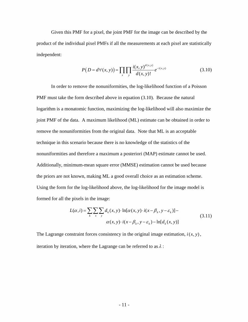
Given this PMF for a pixel, the joint PMF for the image can be described by the
product of the individual pixel PMFs if all the measurements at each pixel are statistically
independent:
( )( , )
( , )( , )( , )( , )!
d x yi x y
x y
i x yP D d x y ed x y
−= ∀ =∏∏ (3.10)
In order to remove the nonuniformities, the log-likelihood function of a Poisson
PMF must take the form described above in equation (3.10). Because the natural
logarithm is a monatomic function, maximizing the log-likelihood will also maximize the
joint PMF of the data. A maximum likelihood (ML) estimate can be obtained in order to
remove the nonuniformities from the original data. Note that ML is an acceptable
technique in this scenario because there is no knowledge of the statistics of the
nonuniformities and therefore a maximum a posteriori (MAP) estimate cannot be used.
Additionally, minimum-mean square error (MMSE) estimation cannot be used because
the priors are not known, making ML a good overall choice as an estimation scheme.
Using the form for the log-likelihood above, the log-likelihood for the image model is
formed for all the pixels in the image:
( , ) ( , ) ln[ ( , ) ( , )]
( , ) ( , ) ln[ ( , )]
k kk x y
k k k
L i d x y x y i x y k
x y i x y d x y
α α
α β ε
= ⋅ ⋅ −
⋅ − − −
∑∑∑ β ε− − (3.11)
The Lagrange constraint forces consistency in the original image estimation, i ( , )x y ,
iteration by iteration, where the Lagrange can be referred to asλ :
- 11 -

( , ) ( , ) ln[ ( , ) ( , )]
( , ) ( , ) ( , )
k kk x y
k kx y
L i d x y x y i x y k
x y i x y i x y
α α
α β ε λ
= ⋅ ⋅ −
⋅ − − −
∑∑∑
∑∑
β ε− −
(3.12)
Now the derivative of the log-likelihood described in equation (3.12) is taken with
respect to the gain nonuniformity for one pixel. Note that the derivative of the last term
in equation (3.12) is zero because it does not have gain:
( )
0 0 0 0
0 0 0 0
( ( , )) ( , ) ln[ ( , ) ( , )]( ( , )) ( ( , ))
( , ) ( , ) ( , )( ( , )) ( ( , ))
k kk x y
k kx y
L i d x y x y i x yx y x y k
x y i x y i x yx y x y
α α β εα α
α β ε λα α
⎛ ⎞∂ ∂= ⋅ ⋅ −⎜ ⎟∂ ∂ ⎝ ⎠
⎛ ⎞∂ ∂− ⋅ − − − ⎜ ⎟∂ ∂ ⎝ ⎠
∑∑∑
∑∑
−
(3.13)
Set the result of the derivative in equation (3.13) equal to zero and solve for the
gain at pixel, 0 0( , )x y :
0 00 0
0 0
( , )0 ( ,( , )
kk k
k
d x y i x yx y
)β εα
⎛ ⎞= − −⎜
⎝ ⎠∑ − ⎟ (3.14)
Distribute the sum over k:
0 0
0 00 0
( , )0 (
( , )
kk
kk
d x yi x y
x y, )kβ ε
α= − −∑
∑ − (3.15)
A simple example with k summing from 1 to 2 demonstrates the mathematics
used:
1 0 0 2 0 00 1 0 1 0 2 0 2
0 0 0 0
( , ) ( , )0 ( , ) (( , ) ( , )
d x y d x y i x y i x yx y x y
, )β ε βα α
= + − − − − − ε− (3.16)
Pull gain nonuniformity, α , out of the sum over d below:
( )1 0 0 2 0 0 0 1 0 1 0 2 0 20 0
10 ( , ) ( , ) ( , ) ( ,( , )
d x y d x y i x y i x yx y
)β ε βα
= + − − − − − ε− (3.17)
- 12 -

Move the image, i, to the left side of the equation:
( )0 1 0 1 0 2 0 2 1 0 0 2 0 00 0
1( , ) ( , ) ( , ) ( ,( , )
i x y i x y d x y d x yx y
β ε β εα
− − + − − = + ) (3.18)
Solve for the gain, alpha:
( )1 0 0 2 0 00 0
0 1 0 1 0 2 0 2
( , ) ( , )( , )
( , ) ( ,d x y d x y
x yi x y i x y
α)β ε β
+=
− − + − −ε (3.19)
Translate back having sums over k in the numerator and denominator to show the
final result for the gain nonuniformities:
0 0
0 00 0
( , )( , )
( ,
kk
k kk
d x yx y
i x yα
)β ε=
− −
∑∑
(3.20)
Now, substitute equation (3.20) into equation (3.12) to create a log likelihood
equation based solely on the image as shown:
1
1
2 2
2
3
3
4 4
4
( , ) ( , )( ) ( , ) ln
( , )
( , ) ( , )( , )
( , )
k kk
kk x y k k
k
k k kk
k x y x yk kk
d x y i x yL i d x y
i x y
d x y i x yi x y
i x y
kβ ε
β ε
β ελ
β ε
⎡ ⎤⋅ − −⎢ ⎥= ⋅ ⎢ ⎥− −⎢ ⎥⎣ ⎦
⋅ − −− −
− −⋅
∑∑∑∑ ∑
∑∑∑∑ ∑∑∑
(3.21)
Now differentiate equation (3.21) with respect to the image and set to zero:
0 0 0 0 0 0 0 0
( ( )) (1 Term) (2 Term) (3 Term)( ( , )) ( ( , )) ( ( , )) ( ( , ))
st nd rdL ii i i iγ η γ η γ η γ η∂ ∂ ∂ ∂
= + +∂ ∂ ∂ ∂
(3.22)
In order to simplify the derivative operation the derivative of each term is
demonstrated individually, where the first term using the notation described above can be
expressed as:
- 13 -

1
1
2 2
2
0 0 0 0
(1 Term) ( , )( ( , )) ( ( , ))
( , ) ( , ) ln
( , )
st
kk x y
k kk
k kk
d x yi i
d x y i x y
i x y
γ η γ η
kβ ε
β ε
∂ ∂= ⋅ ⋅
∂ ∂
⎡ ⎤⋅ − −⎢ ⎥⎢ ⎥− −⎢ ⎥⎣ ⎦
∑∑∑
∑∑
(3.23)
Where a simplification of the first term results as shown below using the
properties of the natural log:
[ ]
1
1
2 2
20 0
ln ( , )
( , ) ln ( , )( ( , ))
ln ( , )
kk
k kk x y k
k k
d x y
d x y i x yi
i x y
β εγ η
β ε
k
⎧ ⎫⎡ ⎤⎪ ⎪⎢ ⎥⎪ ⎪⎣ ⎦⎪ ⎪⎡ ⎤∂ ⎪ ⎪= ⋅ ⋅ − − −⎨ ⎬⎢ ⎥∂ ⎣ ⎦⎪ ⎪⎪ ⎪+ − −⎪ ⎪⎪ ⎪⎩ ⎭
∑
∑∑∑ ∑ (3.24)
Where the derivative with respect to the image of the first part inside the brackets
of equation (3.24) above is equal to zero because there is no image, and simply a
derivative of a constant:
1
10 0
( , ) ln ( , ) 0( ( , )) k k
k x y kd x y d x y
i γ η⎡ ⎤∂
=⎢∂ ⎣ ⎦∑∑∑ ∑ ⎥ (3.25)
The derivative of the third part inside the brackets of equation (3.24) above is the
next most challenging and can be described as shown below in equation (3.26):
[ ]
[ ]0 0
0 0
( , ) ln ( , )( ( , ))
( , ) ln ( , )( ( , ))
k k kk x y
k kk x y
d x y i x yi
d x y i x yi
β εγ η
kβ εγ η
∂⋅ − − =
∂
∂⋅ − −
∂
∑∑∑
∑∑∑ (3.26)
And can be further simplified using the chain rule:
- 14 -

[ ]
[ ]0 0
0 0
( , ) ln ( , )( ( , ))
( , ) ( , )( , ) ( ( , ))
k k kk x y
kk k
k x y k k
d x y i x yi
d x y i x yi x y i
β εγ η
β εβ ε γ η
∂⋅ − − =
∂
∂⋅ − −
− − ∂
∑∑∑
∑∑∑ (3.27)
Where the rightmost statement in equation (3.27) can be calculated as follows:
[ ]0 0 0 0
( , ) ( , )( , )
( ( , )) ( , )
k k
k k
i x yi x y
i iγ η
γ η δ γ β η εβ ε
γ η γ η
∂ ⋅ ⋅ − − − −∂
− − =∂ ∂ ⋅
∑∑ (3.28)
The derivative taken of the image at any other point other than 0 0( , )i γ η is zero
and the single remaining point is:
[ ] 0 0 0 0
0 0 0 0
( , ) ( , )( , )( ( , )) ( , )
kk k
i x yi x yi i
kγ η δ γ β η εβ εγ η γ η
∂ ⋅ ⋅ − − − −∂− − =
∂ ∂ ⋅ (3.29)
Resulting in just the shifted delta function:
[ ] 0 00 0
( , ) ( ,( ( , )) k k ki x y x yi
)kβ ε δ γ β η εγ η∂
− − = − − − −∂
(3.30)
Making the result of the third part in the brackets of equation (3.24):
[ ]
0 0
0 0
( , ) ln ( , )( ( , ))
( , ) ( , )( , )
k k kk x y
kk k
k x y k k
d x y i x yi
d x y x yi x y
β εγ η
δ γ β η εβ ε
∂⋅ − − =
∂
⋅ − − − −− −
∑∑∑
∑∑∑ (3.31)
The second part in the brackets of equation (3.24) can be described as:
2 2
2
2 2
2
0 0
0 0
( , ) ln ( , )( ( , ))
( 1) ( , ) ln ( , )( ( , ))
k k kk x y k
k kk x y k
d x y i x yi
d x y i x yi
β εγ η
β εγ η
⎡ ⎤∂⋅ − − − =⎢ ⎥∂ ⎣ ⎦
k
⎡ ⎤∂− ⋅ ⋅ − −⎢ ⎥∂ ⎣ ⎦
∑∑∑ ∑
∑∑∑ ∑(3.32)
Where the second part in brackets of equation (3.24) above is simplified to a very
similar form found in the third part in brackets of equation (3.24), having a sum of the
- 15 -

images over k inside the natural log instead of just one shifted image. Using this
similarity and the process described above in equations (3.26)–(3.31), the final answer for
the second part in brackets of equation (3.24) can be found as:
2 2
2
2
2
2 2
22 2
2
0 0
0 0
( , ) ln ( , )( ( , ))
( , ) ( 1) ( , )
( , )
k k kk x y k
kk
k kk x y kk k
k
d x y i x yi
d x yx y
i x y
β εγ η
δ γ β η εβ ε
⎡ ⎤∂⋅ − − − =⎢ ⎥∂ ⎣ ⎦
− ⋅ − −− −
∑∑∑ ∑
∑∑∑∑ ∑∑
− −
(3.33)
Putting equation (3.25) – (3.33) together, the final derivative of the first term of
equation (3.22) is:
2
2
2 2
22 2
2
0 00 0
0 0
( , )(1 Term) ( , )( ( , )) ( , )
( , ) ( , )
( , )
stk
k kk x y k k
kk
k kk x y kk k
k
d x y x yi i x y
d x yx y
i x y
δ γ β η εγ η β ε
δ γ β η εβ ε
∂= ⋅ − − − −
∂ − −
− ⋅ − −− −
∑∑∑
∑∑∑∑ ∑∑
− −
(3.34)
The derivative of the second term using the notation described above in equation
(3.21) and equation (3.22) is expressed as:
3
3
4 4
4
0 0 0 0
( , ) ( , )(2 Term) ( 1)( ( , )) ( ( , )) ( , )
k kndk
k x y k kk
d x y i x y
i i i x y
kβ ε
γ η γ η β ε
⋅ − −∂ ∂
= ⋅ −∂ ∂ − −
∑∑∑∑ ∑
(3.35)
Where the shifted images can be expressed using equation (3.7):
3
3
4 4
4
0 0 0 0
(2 Term) ( 1)( ( , )) ( ( , ))
( , ) ( , ) ( , )
( , ) ( , )
nd
k kk
k x y k kk
i id x y i x y
i x yγ η
γ η
γ η γ η
kγ η δ γ β η ε
γ η δ γ β η ε
∂ − ⋅∂=
∂ ∂
⋅ ⋅ − − −
⋅ − − − −
∑ ∑∑∑∑∑ ∑∑∑
− (3.36)
- 16 -

The derivative with respect to 0 0( , )i γ η for any image pixel outside 0 0( , )γ η is
zero making all terms not at location 0 0( , )γ η go to zero:
3
3
4 4
4
0 0 0 0
0 0 0 0
0 0 0 0
(2 Term) ( 1)( ( , )) ( ( , ))
( , ) ( , ) ( , )
( , ) ( , )
nd
k kk
k x y k kk
i id x y i x y
i x y
γ η γ η
kγ η δ γ β η ε
γ η δ γ β η ε
∂ − ⋅∂=
∂ ∂
⋅ ⋅ − − − −
⋅ − − − −
∑∑∑∑ ∑
(3.37)
And can be simplified as:
3
0 0
0 0
(2 Term)( ( , ))
( 1) ( , ) 1( ( , ))
nd
kk x y
i
d x yi
γ η
γ η
∂=
∂∂
− ⋅ ⋅ ⋅∂∑∑∑
(3.38)
Giving the simple result for the second term of zero:
0 0
(2 Term) 0( ( , ))
nd
i γ η∂
=∂
(3.39)
The derivative of the third term is also rather simple, as there is only a λ with the
sum of the image:
0 0 0 0
(3 Term) ( 1) ( , )( ( , )) ( ( , ))
nd
x y
i x yi i
λγ η γ η
∂ ∂= ⋅ − ⋅ ⋅
∂ ∂ ∑∑ (3.40)
Where the derivative of sum over x and y with the image goes to 1 and leaves the
constant λ :
0 0 0 0
(3 Term) ( 1) (1)( ( , )) ( ( , ))
nd
i iλ
γ η γ η∂ ∂
= ⋅ − ⋅ ⋅∂ ∂
(3.41)
Giving the final result for the third term of equation (3.22):
- 17 -

0 0
(3 Term) ( 1) ( )( ( , ))
nd
iλ λ
γ η∂
= − ⋅ = −∂
(3.42)
Putting the first, second and third terms in equation (3.34), equation (3.39) and
equation (3.42) together to give the final result:
2
2
2
2
0 00 0
0 0
( , )( ( )) ( , )( ( , )) ( , )
( , ) ( , )
( , )
kk k
k x y k k
kk
k kk x y kk k
k
d x yL i x yi i x y
d x yx y
i x y
δ γ β η εγ η β ε
δ γ β η εβ ε
∂= ⋅ − − − −
∂ − −
− ⋅ − −− −
∑∑∑
∑∑∑∑ ∑∑
λ− − − (3.43)
Using equation (3.43) the derivative of the log likelihood with respect to the
image is taken and set equal to zero maximizing for the image as described above and
giving rise to an iterative solution:
2
2
2
2
0 0
0 0
( , )0 ( , )( , )
( , ) ( , )
( , )
kk k
k x y k k
kk
k kk x y kk k
k
d x y x yi x y
d x yx y
i x y
δ γ β η εβ ε
δ γ β η εβ ε
= ⋅ − − − −− −
− ⋅ − −− −
∑∑∑
∑∑∑∑ ∑∑
λ− − − (3.44)
Where the iterative solution for the image using equation (3.44) is:
2
2
2
2
0 0
0 0
0 0
0 0
( , )
( , ) ( , )( , )
( , )( , )
( ,( , )
new
kk k
k x y k kold
kk
k kk x y kk k
k
i
d x y x yi x y
id x y
x yi x y
)
γ η
δ γ β η ε λβ ε
γ η
δ γ β η εβ ε
=
⎡ ⎤⎢ ⎥⎢ ⎥⋅ − − − − −⎢ ⎥− −⎢ ⎥⎢ ⎥⎢ ⎥⋅ − − − −⎢ ⎥− −⎢ ⎥⎣ ⎦
∑∑∑∑
∑∑∑ ∑∑
(3.45)
This iterative solution is set up as shown because the elements in equation (3.44)
are a positive gradient, negative gradient, and the Lagrange, and forming an iterative
- 18 -

solution that is multiplicative verses additive will ensure that the image never goes
negative, as demonstrated in Richardson [7]. This is important because the image is in
units of photons. Making the multiplier a ratio of the positive gradient over the negative
gradient moves the old image closer to the ML estimate iteration by iteration.
In order to simplify the expression the equation can be broken down into what
will be referred to in this document as the numerator and denominator:
0 0 0 0( , )Numerator ( , ) ( , )
( , )k
k kk x y k k
d x ynum x yi x y
γ η δ γβ ε
= = ⋅ − − −− −∑∑∑ β η ε− (3.46)
2
2
2
2
0 0
0 0
Denominator ( , )( , )
( , )( , )
kk
k kk x y kk k
k
dend x y
x yi x y
γ η
δ γ β η εβ ε
= =
⋅ − − − −− −
∑∑∑∑ ∑∑
(3.47)
With these expressions the equation can be simplified as:
0 00 0 0 0
0 0
( , )( , ) ( , )( , )new old
numi iden
γ η λγ η γ ηγ η
⎡ ⎤−= ⋅ ⎢ ⎥
⎣ ⎦ (3.48)
The Lagrange multiplier needs to be adjusted for each iteration and can be solved
for as demonstrated below. As shown, it is simplified in terms of the numerator and
denominator described by equation (3.46) and equation (3.47):
0 00 0 0 0 0 0
0 0 0 0
( , )( , ) ( , ) ( , )( , ) ( , )new old old
numi i iden den
γ η λγ η γ η γ ηγ η γ
= ⋅ − ⋅η
(3.49)
Where the resulting solution for the Lagrange multiplier is:
0 0 0 0
0 0
0 0
0 0
( , ) ( , ) ( , )( , )
( , )( , )
old k
k x y
old
i num d x yden
iden
γ η γ ηγ η
λγ ηγ η
⋅−
Κ=
⎛ ⎞⎜ ⎟⎝ ⎠
∑∑∑ (3.50)
- 19 -

This notation is especially helpful for coding practices as the numerator and the
denominator need to be calculated for each iteration, then the value forλ is found with
the numerator and denominator, and lastly the same numerator and denominator are used
with the newλ in order to find 0 0( , )newi γ η .
As the iteration starts, an initial starting value for 0 0( , )oldi γ η must be found. The
algorithm will not run to completion with a continually decreasing MSE if zeros or ones
are used as starting place for 0 0( , )oldi γ η .
The first estimate for 0 0( , )oldi γ η is the average result of the frames with the shifts
included and can be described as:
( ,
( , )k k
kstart
d x yi x y
)kβ η− −=
Κ
∑ (3.51)
As a reminder, from equations (3.11) through (3.43) it can be seen that the log-
likelihood with respect to the gain nonuniformities is found by taking the derivative of
the log-likelihood with respect to the nonuniformities, setting it equal to zero, and then
rearranging the result to find the nonuniformities with the result, as shown above:
0 00 0
( , )( , )
( ,
kk
k kk
d x y
iα γ ε
)γ β ε ε=
− −
∑∑
(3.20)
This description of the nonuniformities can be used to describe the array
characteristics as well as used to derive the stopping criteria during the iteration process
to find the nonuniformities.
- 20 -

Requirements of Algorithm
This algorithm requires a data cube with shifts that can be determined from the
scene data, or scene data with the shifts in x and y are already provided. In the event
shifts are not known, or cannot be found, this algorithm is not applicable. Knowing this,
methods for shift estimation are used, however shift estimation is not discussed in great
detail during the derivation of this algorithm.
For the purposes of testing this algorithm with measured data, a shift estimation
technique using two frames is used, and can be described generally by the correlation in
both dimensions between a reference image and the shifted image, with the resulting
estimated shift being where the correlation between frames was at its peak in each
dimension. A reference for shift estimation can be found in Robinson and Milanfar for
additional information as well as other shift estimation techniques [8].
In addition, the implementation requires that the magnitude of the shifts be greater
than one-half of a pixel as the algorithm was derived solely with whole pixel shifts in
mind, and a pixel shift of magnitudes one-half or less will not come to a desirable
solution for the original image. This requirement arises from the need for each pixel to
see a different part of the scene with the same nonuniformity. An example of the
dependence on accurate shifts of greater than one-half of a pixel in magnitude is shown in
the results section and shows that ideally, whole shifts and accurate estimation of those
shifts would result in the best performance.
- 21 -

It should be noted that empty scenes (and the corresponding sections of the FPA)
will only contain bias data and will not produce favorable results in terms of
nonuniformity estimation and correction without additional information from those pixels
in the FPA.
In terms of scene content, the data cube to be used should also have image data in
terms of received photons, and if not, the data should be converted to the number of
received photons in order to estimate nonuniformities, and that the data cube not contain
zeros or negative numbers as the estimate makes the assumption that there is always
some bias for each detector.
It should also be noted that this algorithm corrects for dead pixels (pixels that
return a near-zero response regardless of scene input) and naturally removes these dead
pixels, assuming that the shifted data provides enough information to correct for the dead
pixel. For example, if a 3x3 area of pixels is dead and the available image data only has
shifts of up to 1 pixel in any direction, the dead pixel area will not be completely
corrected with this algorithm.
Again, this algorithm implementation is derived specifically for integer shifts. If
a data cube possesses subpixel shifts the shift data used in the algorithm should be
rounded to the nearest whole shift as mentioned above. This gives rise to the requirement
above for the magnitude of shifts to be greater than a half-pixel in each direction in order
to estimate the nonuniformities in addition to having the input shifts as whole pixels.
- 22 -

Derivation of Stopping Criteria
During calibration of real LIDAR data the original scene is not known, therefore
there must be some metric for deciding when to stop the iteration process. This metric
must use data that is available with a realistic scenario. In LIDAR, the bias before signal
return is recorded and the scene imagery itself with shifts must be used to stop the
iteration to find a satisfactory result.
Assuming Poisson noise in the original scene, the mean of the Poisson noise is
equal to the variance of the same.
The average estimated noise variance can be determined by:
( )2( , ) ( , ) ( , )
Noise VarianceY
k new newk x y
d x y x y i x yα− ⋅=
Κ ⋅Χ ⋅
∑∑∑ (3.52)
And the mean can be described by the following:
( )( , )
MeanY
kk x y
d x y=
Κ ⋅Χ ⋅
∑∑∑ (3.53)
If the average variance is less than the average mean the iteration is terminated
because the average variance shows that an improvement have been made to the image,
giving rise to the stopping criteria:
(3.54) ( )2( , ) ( , ) ( , ) ( , )k new new kk x y k x y
d x y x y i x y d x yα− ⋅ <∑∑∑ ∑∑∑( )
- 23 -

Where ( , )new x yα are the estimated nonuniformities, and , , and YΚ Χ are the
number of frames, the length of x, and the length of y, respectively. When the above
equation becomes true the algorithm terminated.
- 24 -

IV. Results of Algorithm
In order to test the new algorithm a simple noiseless case was created with a
simple ramp scene in one dimension. After the algorithm worked with the noiseless case,
Poisson noise was added to the one dimensional ramp and the algorithm was tested again.
Afterward, a two dimensional ramp case was tested without Poisson noise, and then with.
For completeness, another two dimensional test scene was created with sinusoids and is
shown below. These cases were necessary in order to test and validate the model and test
derived stopping methods. In all cases the gain nonuniformities varied uniformly from
0.9 to 1.1. A brief study of the algorithm’s dependence on accurate shift estimates is also
included at the end of this chapter.
1D No Noise Performance
A one dimensional noiseless case was the first test applied to the derived
algorithm. This case was used as a test method and has aided significantly in algorithm
development and testing. This one dimensional case contained a scene with a simple
intensity ramp and low values on the outer edges. The maximum value for the ramp was
300,000 units, based on a value that would approximate a maximum well depth (Well
depth being the maximum number of photons before a readout is necessary.) for photons
in a sensor. The final image fed to the algorithm consisted of the original scene data
multiplied by the nonuniformities as shown below:
( , ) ( , ) ( , ) ( , )k k kd x y i x y x y n x yβ ε ηυ= − − ⋅ + (4.1)
- 25 -
Where represents the image with gain nonuniformities, ( )kd x ( )ki x β−
represents the original scene shifted by the kth shift in x, and ( )xηυ represents the gain
nonuniformities in the focal plane array.
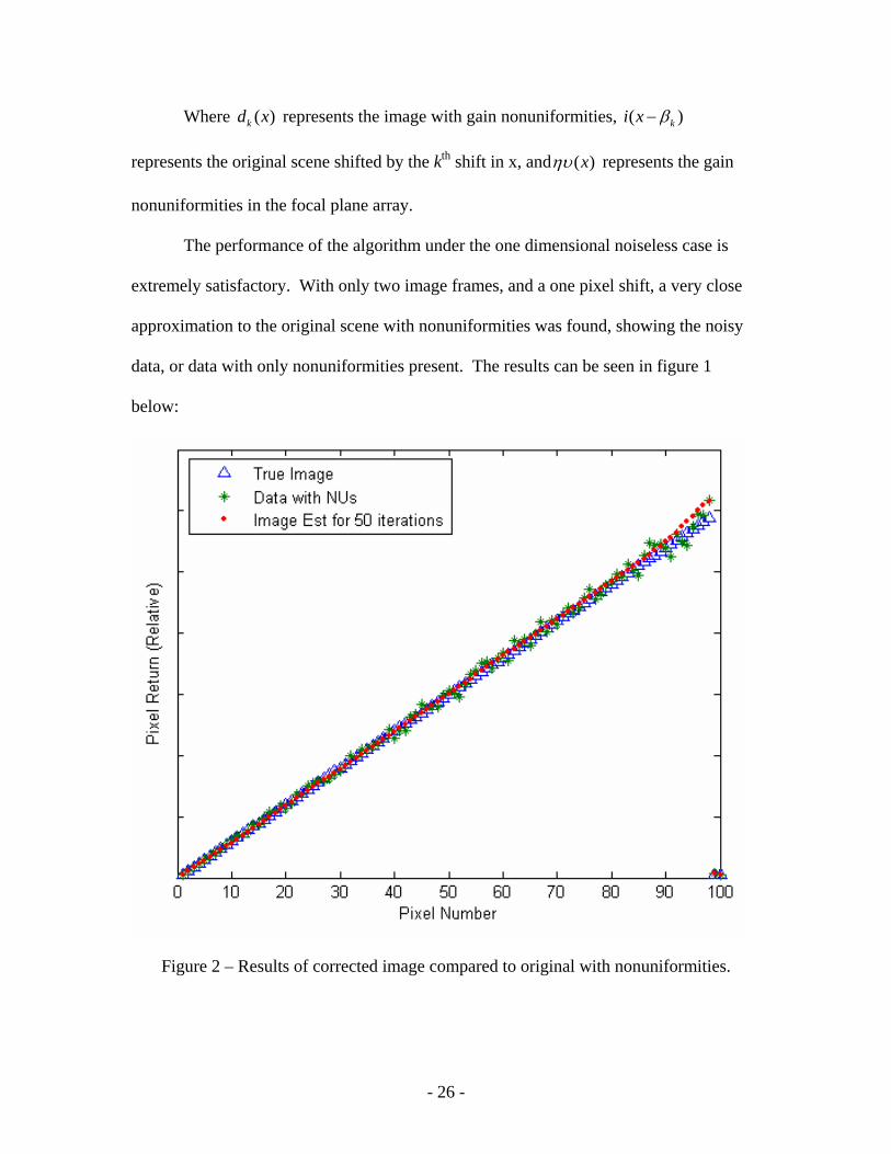
The performance of the algorithm under the one dimensional noiseless case is
extremely satisfactory. With only two image frames, and a one pixel shift, a very close
approximation to the original scene with nonuniformities was found, showing the noisy
data, or data with only nonuniformities present. The results can be seen in figure 1
below:
Figure 2 – Results of corrected image compared to original with nonuniformities.
- 26 -

It can be seen in figure 2 above that the corrected one dimensional image is a
much closer match to the true image than the noisy data (data with nonuniformities, no
Poisson noise). The shift between the two frames used in this example is simply 1 and
the result in figure 2 and 3 resulted after 50 iterations.
As the algorithm is iterated the MSE (Mean Squared Error) is reduced iteration by
iteration and eventually bottoms out, as shown in figures 3 and 5:
Figure 3 – Running MSE (Mean Square Error) iteration by iteration.
Figure 3 above is a Log-Log figure corresponding to the MSE for figure 2, it
appears from a limited number of iterations the MSE appears to go down as the iteration
- 27 -

number increases, but after many iterations the MSE does reach a minima, as shown in
figure 5.
With increased iterations the performance of the algorithm continues to improve
the overall image and the MSE continues to be reduced, as shown in figure 4:
Figure 4 – One dimensional test case with many iterations and no Poisson noise.
It can be seen in figure 4 that with even more iterations the resulting image
quality is improved even more. This is especially evident when figure 4 is compared to
the error seen in figure 2 in the upper right corner.
- 28 -

As the algorithm is iterated to an even higher number the MSE is reduced even
further and eventually bottoms out. This can be seen in the following figure:
Figure 5 – Resulting MSE from no Poisson noise case with many iterations.
It can be seen by the log-log plot in figure 5 that the corresponding to the MSE
that results after producing figure 4 that the MSE is reaches a minima after roughly 5000
iterations and runs to roughly 10,000 iterations as shown in figure 4.
While it may not be evident in figure 3 that the MSE contains a minima, with only
quantization noise and nonuniformities the MSE does reach a minima after roughly 5000
iterations as shown in figure 5. Note that this would be the optimum stopping point for
- 29 -

the algorithm. Figures with Poisson noise hereafter will demonstrate the stopping
criteria.
1D With Poisson Noise Performance
After the testing without noise was completed the algorithm was tested with
Poisson noise. The image with Poisson noise was then processed by the algorithm and
the results can be seen below in figure 6:
Figure 6 – Resulting image with Poisson noise after 5000 iterations.
- 30 -
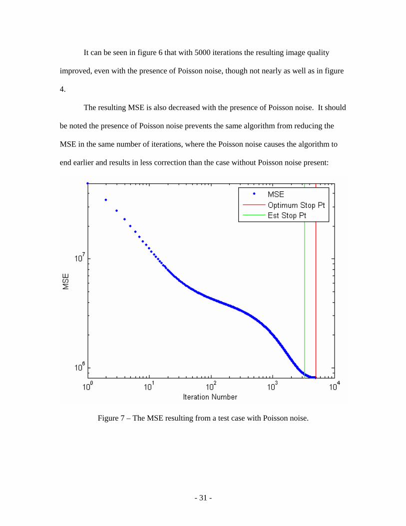
It can be seen in figure 6 that with 5000 iterations the resulting image quality
improved, even with the presence of Poisson noise, though not nearly as well as in figure
4.
The resulting MSE is also decreased with the presence of Poisson noise. It should
be noted the presence of Poisson noise prevents the same algorithm from reducing the
MSE in the same number of iterations, where the Poisson noise causes the algorithm to
end earlier and results in less correction than the case without Poisson noise present:
Figure 7 – The MSE resulting from a test case with Poisson noise.
- 31 -

In the log-log plot on figure 7 it can be seen with that the algorithm does not
perform as well with Poisson noise than without it. It can also be seen that the MSE
bottoms out after many iterations, with the stopping criteria ending at 4000 iterations
while the optimum stopping point would be at 3000 iterations.
Figure 7 reveals characteristics of the MSE verses iteration number, showing that
the image reaches a best case with noise and then if the iteration continues the resulting
image quality is reduced. If allowed to continue the MSE will continue to rise.
2D No Noise Performance
For the two dimensional case without Poisson noise a two dimensional ramp
similar to the one dimensional case with a maximum value of 300,000 units at the
maximum corner and near-zero at the minimum corner. Just as with the no Poisson noise
one dimensional case, the two dimensional case produces very favorable results as seen
by a slice of the image through the 50th row:
- 32 -

Figure 8 – 2D ramp without Poisson noise.
Figure 8 shows a slice through the two dimensional ramp it can be seen in the
corrected one dimensional image that the dots representing the estimated image are a
much closer matching to the true image than the noisy data with nonuniformities.
The resulting MSE is also very favorable as evidenced by the following plot:
- 33 -

Figure 9 - The resulting MSE for the 2 dimensional ramp without Poisson noise.
In figure 9 the MSE appears to be decreasing iteration by iteration. As with the
one dimensional case the MSE does bottom out after many thousands of iterations,
although not obvious from this figure.
The nonuniformities in the images themselves and the corrected image using the
algorithm can be seen by the comparative illustration below:
- 34 -

Figure 10 - An illustration with the 2D test ramp with and without nonuniformities.
Figure 10 shows a comparative illustration of the test ramp with nonuniformities
showing the image with nonuniformities on the left and the corrected image on the right.
Note that there is no Poisson noise in this case, giving a very favorable result.
2D With Noise Performance
For the two dimensional noise case a two dimensional ramp similar to the one
dimensional case with a maximum value of 300,000 units at the maximum corner and
near-zero at the minimum corner as mentioned above. Using this same image, Poisson
noise is included in each frame of the image series and the resulting frames are processed
by the algorithm. Just as with the one dimensional case with Poisson noise, the two
dimensional case produces favorable results as seen by a slice of the image through the
50th row of the image:
- 35 -

Figure 11 – 2D ramp with Poisson noise.
The image slice in figure 11 above demonstrates a portion of the corrected two
dimensional image with Poisson noise present. Note the lower performance compared to
the case without Poisson noise.
The resulting MSE is also very favorable as evidenced by the following plot with
the stopping criteria ending slightly prematurely but very close to the minimum MSE:
- 36 -

Figure 12 – The MSE resulting from the 2D test ramp with Poisson noise.
The resulting log-log MSE in figure 12 above shows excellent performance
iteration by iteration until it reaches a minima after roughly 1000 iterations while the
stopping criteria stops the iteration after roughly 200 iterations with this relatively low
level of Poisson noise.
The nonuniformities in the images themselves and the corrected image using the
algorithm can be seen by the comparative illustration below:
- 37 -

Figure 13 – An illustration showing images with NUs, NUs and Poisson noise, and the final corrected image.
The comparative illustration in figure 13 above shows the nonuniformities
including two dead pixels, the nonuniformities with Poisson noise, and the resulting
corrected image showing the dead pixels filtered out. Both dead pixels are centered
horizontally, one near the top and the second near the bottom.
Additional 2D Case With Noise
In order to demonstrate that the algorithm works on more than a simple ramp,
another case was prepared to demonstrate the algorithm’s effectiveness. The figure
below shows the performance of this test image with a two dimensional sinusoid:
- 38 -
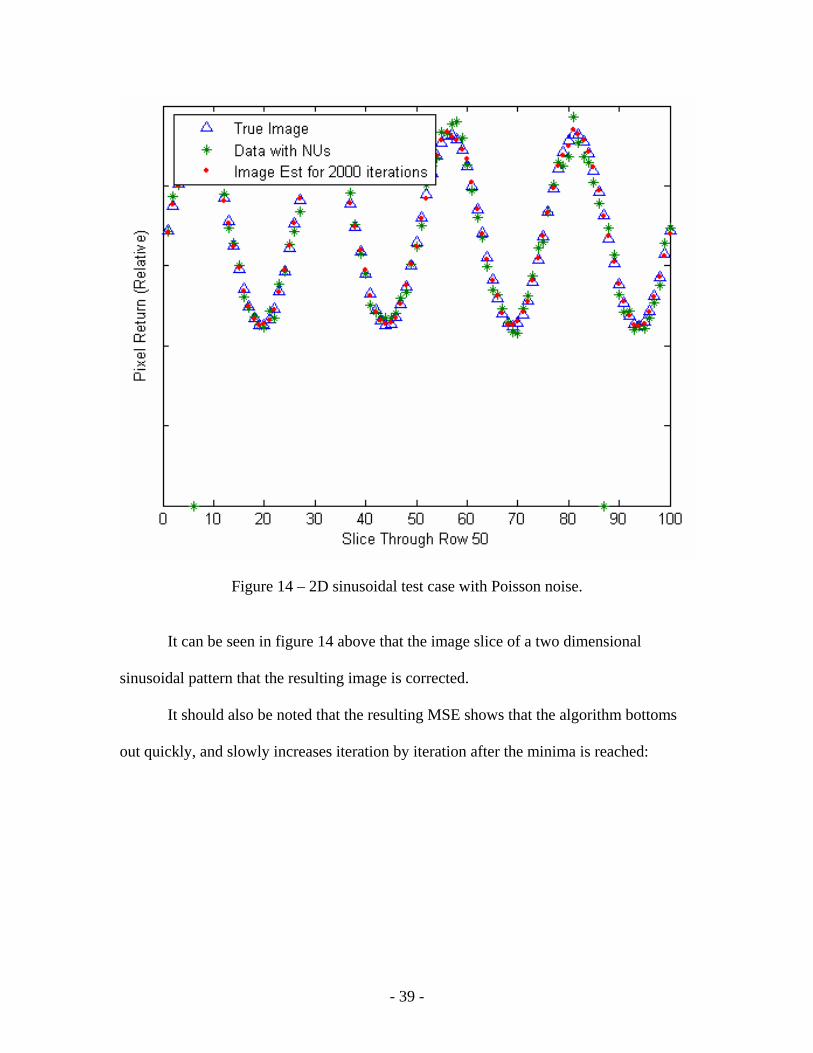
Figure 14 – 2D sinusoidal test case with Poisson noise.
It can be seen in figure 14 above that the image slice of a two dimensional
sinusoidal pattern that the resulting image is corrected.
It should also be noted that the resulting MSE shows that the algorithm bottoms
out quickly, and slowly increases iteration by iteration after the minima is reached:
- 39 -

Figure 15 – MSE that results from 2D sinusoidal test case with Poisson noise.
The resulting MSE in figure 15 bottoms out quickly, and slowly rises over many
iterations where the estimated stopping point stops at roughly 1950 iterations with only a
minimal increase in the MSE still providing an excellent correction.
The resulting images from this two dimensional sinusoidal test case are shown
below where the location of two dead pixels are easily seen in Figure 16:
- 40 -

Figure 16 – An illustration showing the 2D sinusoidal test case with NUs, NUs and Poisson noise, and the corrected image.
It can be seen in figure 16 above that the two dimensional sinusoidal image, even
with two dead pixels, is corrected and the dead pixels are removed.
Overall, the performance of the algorithm on simulated images was excellent,
with the MSE reaching its low point very quickly, and the dead pixels being removed
from the original image.
Algorithm Dependence on Accurate Shift Estimates
The algorithm was derived using whole shifts, and as a result is dependant on
accurate shift inputs and their related input scenes. In order to test the dependence on
accurate shifts, a set of 2D test image pairs with sub-pixel shifts between 0.6 and 1.4
pixels in x and y were generated. Each pair of images was used with an input of a shift in
x and y and the MSE results were compared. The results are shown in the figures
following:
- 41 -

Figure 17 – A demonstration of algorithm sensitivity to accurate shift inputs.
Figure 17 above demonstrates sets of image pairs with real sub-pixel shifts in x
and y ranging from 0.6 to 1.4 pixels. The minimum MSE achieved in each scenario is
plotted showing that the minimum MSE is reached when the shift estimate fed to the
algorithm is closest to the accurate value of the shift. Notice the higher error on shifts of
1.1 to 1.4 because of the nature of the ramp image used to test the scenario.
Notice that the minimum MSE is reached when the shift data fed to the algorithm
is most accurate. This is expected as the algorithm was derived to use whole shifts in
- 42 -
order to optimize for speed. The error introduced by uncertainty in the shifts is highly
dependant on the original image data. This can be seen by the higher error on the right
side of the graph on the figure above due to the original image being a ramp that
increases to the right and down, and a resulting error in the shift down and to the right
increases the relative error between the scenarios.
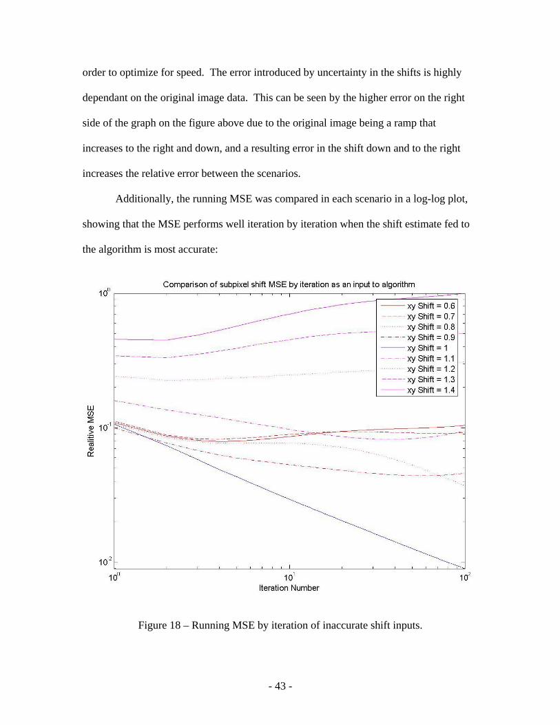
Additionally, the running MSE was compared in each scenario in a log-log plot,
showing that the MSE performs well iteration by iteration when the shift estimate fed to
the algorithm is most accurate:
Figure 18 – Running MSE by iteration of inaccurate shift inputs.
- 43 -

Figure 18 demonstrates the running MSE iteration by iteration with sets of image
pairs with sub-pixel shifts in x and y ranging from 0.6 to 1.4 pixels. The minimum
running MSE is achieved when the shift estimate fed to the algorithm is closest to the
accurate value of the shift. Notice the higher error on shifts of 1.1 to 1.4 shown in
magenta because of the nature of the ramp image used to test the scenario.
The log-log plot in figure 18 also demonstrates the eventual bottoming out of the
MSE, especially when incorrect shifts are inputted into the algorithm. Also note that
while it is not especially visible in figure 18, the 1.0 pixel shift case does bottom out after
many thousands of iterations.
- 44 -

V. Conclusion
Random gain nonuniformities in LIDAR arrays are a problem because of the
nature of these arrays. Because of the nature of LIDAR arrays, having bias data for each
collection, the gain can be corrected with the iterative solution described in this thesis. In
order for this algorithm to operate as implemented, there must be at least a full pixel of
shifts in the horizontal and/or vertical directions between two image frames used as input,
and there must be an accurate estimate of shifts, preferably as close to a whole pixel as
possible.
Having the ability to correct these nonuniformities with a low number of frames
makes the algorithm relatively fast in terms of computation time. This also makes this
algorithm useful to the LIDAR community, improving resulting images.
In test scenarios, the algorithm performs quite well, especially in low-noise cases,
and iterates to a solution that is more favorable than the original image, especially when
the algorithm is stopped at the appropriate iteration. In the event that the algorithm is not
stopped at the appropriate iteration the resulting image could be less favorable than
desired showing little improvement.
It is also important to note that all the test cases were performed knowing the
exact shift between image pairs tested, and those shifts in x and y were whole pixel shifts,
with the exception of the comparison of sub-pixel shift performance where the algorithm
dependence on accurate shift estimation is demonstrated.
It is recommended that for future work that the magnitude of error resulting from
sub pixel shifts is found for real data and the relationship between sub pixel shifts and
- 45 -

algorithm performance is discovered for more than just simulated scenarios. It is also
recommended a sub-pixel version of the algorithm described in this document be derived
and tested in order to compare performance and computational time difference. Work
demonstrating that the algorithm described here could operate in real time along with an
operational LIDAR system could show the additional usefulness of this algorithm.
- 46 -

Bibliography 1. Elkins, William P; Ulich, Bobby L; Lawrence, Jeffrey G; Linton, Harold E. “A 3D
LIDAR Sensor for Volumetric Imaging in Highly Backscattering Media.” Proceedings of SPIE. Volume 5791. 2005.
2. Goodman, Joseph W. Statistical Optics. New York: John Wiley & Sons, Inc. 1985. 3. Hayat, Majeed M; Ratliff, Bradley M; Tyo, J. Scott; Agi, Kamil. “Generalized
Algebraic Scene-based Nonuniformity Correction Algorithm.” Proceedings of SPIE. Volume 5556. 2004.
4. Isoz, Wilhelm. “Nonuniformity correction of infrared focal plane arrays.” Proceedings
of SPIE. Volume 5783. 2005. 5. Leon-Garcia, Alberto. Probability and Random Processes for Electrical Engineering.
Addison-Wesley Publishing Company, Inc. Second Edition. 2004. 6. Morrison, Ryan A; Turner, Jeffrey T; Barwick, Mike; Hardaway, G. Mike. “Urban
reconnaissance with an airborne laser radar.” Proceedings of SPIE. Volume 5791. 2005.
7. Richardson, B. H. “Bayesian-based iterative method of image restoration.” J. Opt. Soc.
Am. Volume 62. pp. 55--59, 1972. 8. Robinson, Dirk and Peyman Milanfar. “Fundamental Performance Limits in Image
Registration.” IEEE Transactions on Image Processing. 13: 1185-1199 (Sept 2004). 9. Su-xia, Xing; Jun-jv, Zhang; Lianjun, Sun; Ben-kang, Chang; Yun-sheng, Qian. “Two
Point Nonuniformity Correction Based on LMS.” Proceedings of SPIE. Volume 5640. 2005.
10. Van Trees, Harry L. Detection, Estimation, And Modulation Theory (Part I). New
York: John Wiley & Sons, Inc., 2001. 11. Wright, Wayne; Hoge, Frank E; Swift, Robert N; Yungel, James K; Schirtzinger, Carl
R. “Next generation NASA airborne oceanographic LIDAR system.” Applied Optics. Volume 40, No 3. 2001.
- 47 -

Vita Christopher A. Rice graduated from Southeastern high school in South
Charleston, Ohio. He completed his undergraduate studies at Cedarville University in
Cedarville, Ohio, earning a Bachelor of Science degree in Electrical Engineering in May
of 2004. Upon graduation, he was awarded full tuition to the Air Force of Technology
(AFIT) in Wright Patterson AFB, Ohio where he was accepted to the Graduate School of
Engineering and Management for a Master’s degree in electrical engineering. Upon
graduation in August of 2006 he will pursue a PhD at AFIT in Engineering Physics.
- 48 -

REPORT DOCUMENTATION PAGE Form Approved OMB No. 074-0188
The public reporting burden for this collection of information is estimated to average 1 hour per response, including the time for reviewing instructions, searching existing data sources, gathering and maintaining the data needed, and completing and reviewing the collection of information. Send comments regarding this burden estimate or any other aspect of the collection of information, including suggestions for reducing this burden to Department of Defense, Washington Headquarters Services, Directorate for Information Operations and Reports (0704-0188), 1215 Jefferson Davis Highway, Suite 1204, Arlington, VA 22202-4302. Respondents should be aware that notwithstanding any other provision of law, no person shall be subject to an penalty for failing to comply with a collection of information if it does not display a currently valid OMB control number. PLEASE DO NOT RETURN YOUR FORM TO THE ABOVE ADDRESS. 1. REPORT DATE (DD-MM-YYYY) 14-09-2006
2. REPORT TYPE Master’s Thesis
3. DATES COVERED (From – To) Aug 2004 – Sept 2006
5a. CONTRACT NUMBER
5b. GRANT NUMBER
4. TITLE AND SUBTITLE Fast Scene Based Nonuniformity Correction with Minimal Temporal Latency 5c. PROGRAM ELEMENT NUMBER
5d. PROJECT NUMBER 5e. TASK NUMBER
6. AUTHOR(S) Rice, Christopher A.
5f. WORK UNIT NUMBER
7. PERFORMING ORGANIZATION NAMES(S) AND ADDRESS(S) Air Force Institute of Technology Graduate School of Engineering and Management (AFIT/EN) 2950 Hobson Way WPAFB OH 45433-7765
8. PERFORMING ORGANIZATION REPORT NUMBER AFIT/GE/ENG/06-59
10. SPONSOR/MONITOR’S ACRONYM(S)
9. SPONSORING/MONITORING AGENCY NAME(S) AND ADDRESS(ES) Richard Richmond AFRL/SNJM Electro-Optics Combat ID Technology Branch; 3109 Hobson Way; WPAFB OH 45433 DSN No: 785-9614 Comm. No: (937) 255-9614
11. SPONSOR/MONITOR’S REPORT NUMBER(S)
12. DISTRIBUTION/AVAILABILITY STATEMENT APPROVED FOR PUBLIC RELEASE; DISTRIBUTION UNLIMITED
13. SUPPLEMENTARY NOTES 14. ABSTRACT The focus of this research was to derive a new algorithm for correction of gain nonuniformities in LIDAR focal plane arrays using as few frames as possible. Because of the current low production rate of LIDAR focal plane arrays there is a natural tendency for extreme nonuniformities to exist on a pixel by pixel basis as the manufacturing technique has not yet been perfected. Generally, nonuniformity correction techniques require a large number of frames and/or have obscure requirements on the translational shifts in the input image frames. This thesis presents a solution for finding multiplicative nonuniformities that exist in a focal plane array and mitigating the effect those nonuniformities.
15. SUBJECT TERMS Nonuniformity Correction, LIDAR, Focal Plane Arrays 16. SECURITY CLASSIFICATION OF:
19a. NAME OF RESPONSIBLE PERSON Stephen Cain, CIV (AFIT/ENG)
REPORT U
ABSTRACT U
c. THIS PAGE U
17. LIMITATION OF ABSTRACT UU
18. NUMBER OF PAGES 58 19b. TELEPHONE NUMBER (Include area code)
(937) 255-6565 x4716; e-mail: [email protected]
Standard Form 298 (Rev: 8-98) Prescribed by ANSI Std. Z39-18
- 49 -
Recommended