Grant No. FA8655-05-1-3053
RIGOROUS MATHEMATICAL MODELING OF ADSORPTION SYSTEM WITH ELECTROTHERMAL
REGENERATION OF THE USED ADSORBENT
Principal investigator:
Dr. Menka Petkovska
Department of Chemical Engineering, Faculty of Technology and Metallurgy, University of Belgrade, Serbia and Montenegro
Other participants on the project: Danijela Antov-Bozalo, Graduate student
Nikola Nikačević, Graduate student
Final Performance Report for Phase 3
3-D COMSOL Multiphysics™ modeling of an adsorber with four parallel annular, radial-flow cartridges
1
Report Documentation Page Form ApprovedOMB No. 0704-0188
Public reporting burden for the collection of information is estimated to average 1 hour per response, including the time for reviewing instructions, searching existing data sources, gathering andmaintaining the data needed, and completing and reviewing the collection of information. Send comments regarding this burden estimate or any other aspect of this collection of information,including suggestions for reducing this burden, to Washington Headquarters Services, Directorate for Information Operations and Reports, 1215 Jefferson Davis Highway, Suite 1204, ArlingtonVA 22202-4302. Respondents should be aware that notwithstanding any other provision of law, no person shall be subject to a penalty for failing to comply with a collection of information if itdoes not display a currently valid OMB control number.
1. REPORT DATE 19 JAN 2006
2. REPORT TYPE N/A
3. DATES COVERED
4. TITLE AND SUBTITLE Rigorous Mathematical Modeling of an Adsorption System WithElectrothermal Regeneration of the Used Adsorbent
5a. CONTRACT NUMBER
5b. GRANT NUMBER
5c. PROGRAM ELEMENT NUMBER
6. AUTHOR(S) 5d. PROJECT NUMBER
5e. TASK NUMBER
5f. WORK UNIT NUMBER
7. PERFORMING ORGANIZATION NAME(S) AND ADDRESS(ES) University of Belgrade Faculty on Technology and Metallurgy Belgrade11000 Yugoslavia
8. PERFORMING ORGANIZATIONREPORT NUMBER
9. SPONSORING/MONITORING AGENCY NAME(S) AND ADDRESS(ES) 10. SPONSOR/MONITOR’S ACRONYM(S)
11. SPONSOR/MONITOR’S REPORT NUMBER(S)
12. DISTRIBUTION/AVAILABILITY STATEMENT Approved for public release, distribution unlimited.
13. SUPPLEMENTARY NOTES The original document contains color images.
14. ABSTRACT
15. SUBJECT TERMS
16. SECURITY CLASSIFICATION OF: 17. LIMITATION OF ABSTRACT
UU
18. NUMBEROF PAGES
44
19a. NAME OFRESPONSIBLE PERSON
a. REPORT unclassified
b. ABSTRACT unclassified
c. THIS PAGE unclassified
Standard Form 298 (Rev. 8-98) Prescribed by ANSI Std Z39-18
PROJECT OVERVIEW
OBJECTIVES The general objective of the project is fundamental mathematical modeling of a complex TSA system with electrothermal desorption step, with adsorbers assembled of one or more cartridge-type, radial flow fixed beds and with in-vessel condensation of the desorbed vapor.
During the first stage of the project, a 1-D mathematical model of a single cartridge without condensation was developed in Matlab and used for simulation. During the second stage of the project, the complete TSA system, for adsorbers with one and two cartridges, was modeled, using a combination of Femlab and Matlab software. 2-D Femlab models that describe adsorption, electrothermal desorption and electrothermal desorption accompanied with condensation of the desorbed vapor were built and integrated using Matlab, in order to describe and simulate complete TSA cycles.
The objective of this, third phase of the project, is to develop mathematical models of another complex configuration, with four parallel annular, radial-flow cartridge-type adsorbers. The analysis of this configuration shows that 3-D models have to be used in order to describe it. The models for adsorption, electrothermal desorption and electrothermal desorption accompanied with condensation of the desorbed vapor are developed again, by using COMSOL Multiphysics (Femlab) 3-D modeling tools.
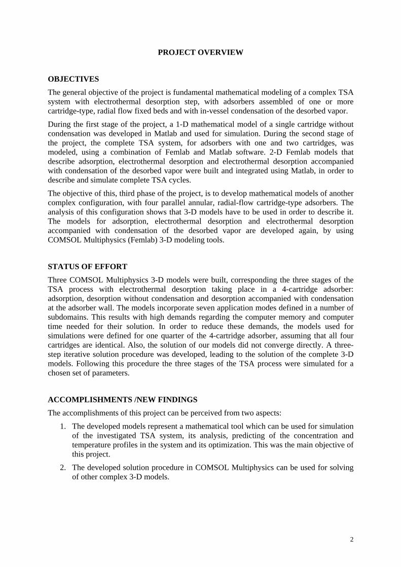
STATUS OF EFFORT Three COMSOL Multiphysics 3-D models were built, corresponding the three stages of the TSA process with electrothermal desorption taking place in a 4-cartridge adsorber: adsorption, desorption without condensation and desorption accompanied with condensation at the adsorber wall. The models incorporate seven application modes defined in a number of subdomains. This results with high demands regarding the computer memory and computer time needed for their solution. In order to reduce these demands, the models used for simulations were defined for one quarter of the 4-cartridge adsorber, assuming that all four cartridges are identical. Also, the solution of our models did not converge directly. A three-step iterative solution procedure was developed, leading to the solution of the complete 3-D models. Following this procedure the three stages of the TSA process were simulated for a chosen set of parameters.
ACCOMPLISHMENTS /NEW FINDINGS The accomplishments of this project can be perceived from two aspects:
1. The developed models represent a mathematical tool which can be used for simulation of the investigated TSA system, its analysis, predicting of the concentration and temperature profiles in the system and its optimization. This was the main objective of this project.
2. The developed solution procedure in COMSOL Multiphysics can be used for solving of other complex 3-D models.
2
PERSONNEL SUPPORTED Danijela Antov-Bozalo, Graduate student
Nikola Nikačević, Graduate student
Dr. Menka Petkovska, Professor
PUBLICATIONS 1. M. Petkovska, D. Antov and P. Sullivan, “Electrothermal desorption in an annular -
radial flow – ACFC adsorber – Mathematical modeling”, Adsorption, 11, 585-590, 2005. (also presented at the FOA-8, 8th International Conference on Fundamentals of Adsorption (FOA8), Sedona, USA, May 23-28, 2004)
2. Petkovska M., Antov-Bozalo D., Marković A. i Sullivan P., “Femlab/Matlab model for complex electric swing adsorption (ESA) system with in-vessel condensation”, Femlab Conference, Oktobar 2005, Stokholm, Proceedings, 117-122
3. Petkovska M., Antov-Bozalo D., Marković A. i Sullivan P. “Electrical swing adsorption (ESA) regenerative filter modeling and simulation”, 2005 Scientific Conference for Chemical and Biological Defense Research, Novembar 2005, Timonium, SAD, Proceedings
4. Antov-Bozalo D., Sullivan P., Petkovska M., “Adsorption and Electrothermal Desorption in Annular - Radial Flow Adsorber – Mathematical Modeling using FEMLAB”, 1st South East European Congress of Chemical Engineering – SEECHE 1, Sept. 2005, Book of Abstracts, 63
In preparation: Two journal and two conference papers
NEW DISCOVERYS, INVENTIONS AND PATENTS: None
3

DETAILED REPORT
1. Introduction
The idea about regeneration of used adsorbents by direct heating of the adsorbent particles by passing electric current through them (Joule effect), was first published in the 1970s [1]. Desorption process based on this principle was later named electrothermal desorption [2]. It was recognized as a prospective way to perform desorption steps of TSA cycles. At the same time, fibrous activated carbon was recognized as a very convenient adsorbent form for its realization. Electrothermal desorption has some advantages over conventional methods, regarding adsorption kinetics and dynamics [3, 4] and energy efficiency [2, 5]. Some industrial applications of electrothermal desorption have been reported recently [6, 7]. Nevertheless, the development of mathematical description of processes based on electrothermal desorption hasn’t been following the development of the process itself, so far.
A new TSA process with electrothermal desorption step, based on adsorbers assembled of one or more annular, cartridge-type, fixed-beds, with in-vessel condensation, has been presented recently [5, 8, 9]. Its schematic representation is given in Figure 1.
Figure 1. Overall schematic representation of the ACFC adsorption – rapid electrothermal desorption system (from Ref. [5])
The aim of this project is to develop rigorous mathematical models of this system for different adsorber configurations. These models could be used for simulation, analysis and optimization of the TSA process developed by Sullivan [5].
1.1. Description of the system The adsorbers of the TSA system shown in Figure 1 are composed of one or more annular, radial-flow cartridge-type adsorbent beds. A single cartridge is schematically shown in Figure 2. It is formed as a cylindrical roll of activated carbon fiber cloth (ACFC), spirally coiled around a porous central pipe. The gas flow through the adsorber is in the radial direction. During the desorption step, electric current is passed through the activated carbon cloth in the axial direction, causing heat generation, heating of the adsorbent and desorption.
4
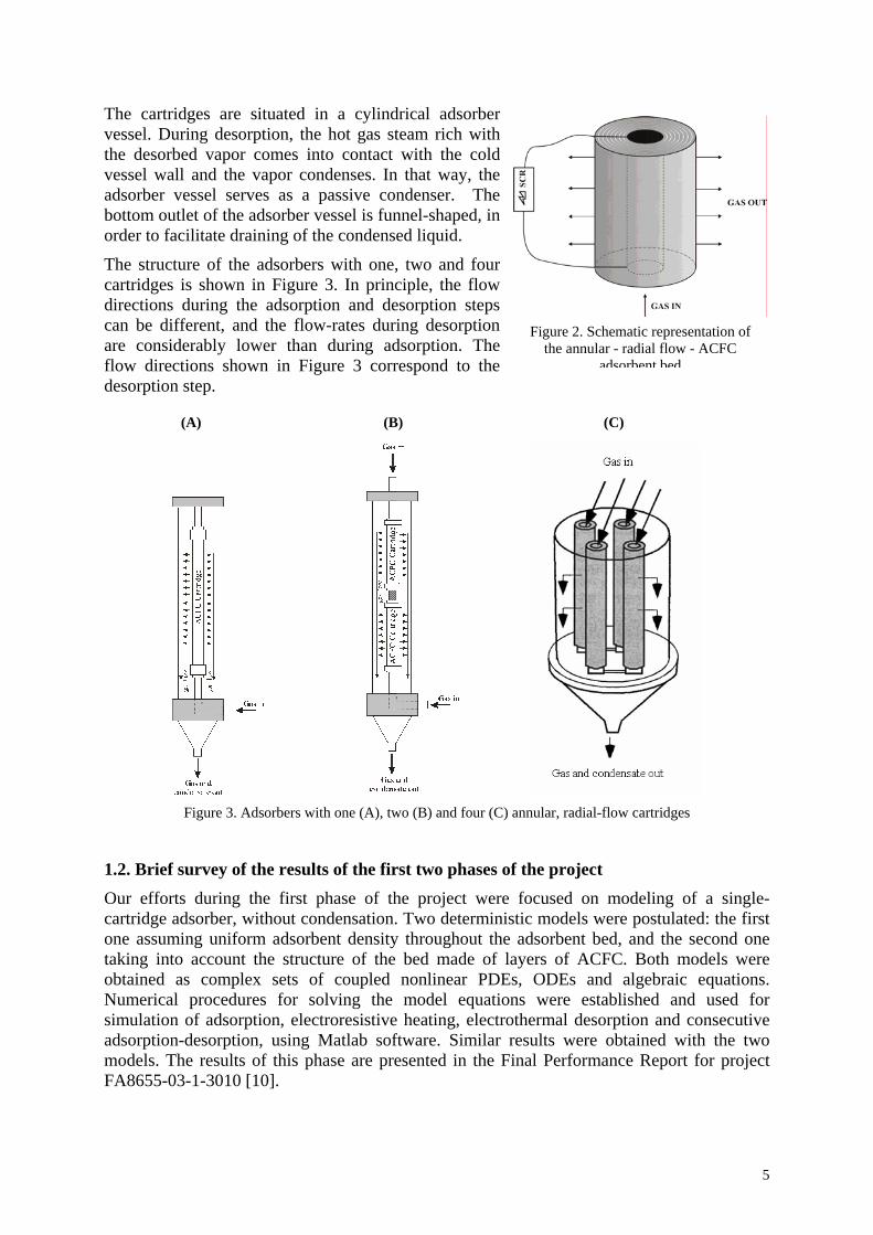
The cartridges are situated in a cylindrical adsorber vessel. During desorption, the hot gas steam rich with the desorbed vapor comes into contact with the cold vessel wall and the vapor condenses. In that way, the adsorber vessel serves as a passive condenser. The bottom outlet of the adsorber vessel is funnel-shaped, in order to facilitate draining of the condensed liquid.
Figure 2. Schematic representation of the annular - radial flow - ACFC
adsorbent bed
The structure of the adsorbers with one, two and four cartridges is shown in Figure 3. In principle, the flow directions during the adsorption and desorption steps can be different, and the flow-rates during desorption are considerably lower than during adsorption. The flow directions shown in Figure 3 correspond to the desorption step.
(C) (B) (A)
Figure 3. Adsorbers with one (A), two (B) and four (C) annular, radial-flow cartridges
1.2. Brief survey of the results of the first two phases of the project
Our efforts during the first phase of the project were focused on modeling of a single- cartridge adsorber, without condensation. Two deterministic models were postulated: the first one assuming uniform adsorbent density throughout the adsorbent bed, and the second one taking into account the structure of the bed made of layers of ACFC. Both models were obtained as complex sets of coupled nonlinear PDEs, ODEs and algebraic equations. Numerical procedures for solving the model equations were established and used for simulation of adsorption, electroresistive heating, electrothermal desorption and consecutive adsorption-desorption, using Matlab software. Similar results were obtained with the two models. The results of this phase are presented in the Final Performance Report for project FA8655-03-1-3010 [10].
5

In the second phase of the project, models for two types of adsorbers, one with only one (Figure 3A), and the other with two cartridges (Figure 3B), have been developed. For each adsorber type, three models were built, in order to describe three stages of a compete ESA cycle: adsorption, electrothermal desorption and electrothermal desorption with in-vessel condensation. These models were built using Femlab, a specialized software tool for modeling of complex systems with complex geometry. The models were defined in 2-D axially symmetrical geometry, with seven application modes. In order to describe the complete TSA cycles, the models for the three stages of the TSA process were integrated, by using a combination of Femlab and Matlab. The models were successfully used for simulation of separate stages of the process and of the complete TSA cycles, as well as for their optimization. The results of this phase are presented in the Final Performance Report for project FA8655-04-1-3053 [11].
1.3. Outline of the third phase of the project The third phase of the project was focused on mathematical modeling of the four-cartridge adsorber, presented in Figure 3C. This configuration has been described in detail in Refs. 10 and 12. This modeling is performed using COMSOL Multiphysics software (previously Femlab). Owing to the complex configuration of this adsorber design, 3-D models have to be used, leading to a number of issues regarding computer memory requirements and convergence problems.
Similarly to the 2-D models developed in the second phase, three 3-D models are needed, to describe three steps of the complete cycle:
- adsorption,
- desorption without condensation,
- desorption accompanied with condensation.
The following application modes were incorporated in these models: Non-isothermal flow, Brinkman Equations, Convection and Diffusion, Diffusion, Convection and Conduction, Heat transfer by Conduction and Conductive Media DC.
Solving of these very complex 3-D models is a rather demanding and difficult task. It assumes optimization of the model structure and geometry definition, the generated mesh and the choice of the solver, in regard to the used hardware, computer time and convergence of the solution.
All these issues were attended in this phase of the project.
2. Modeling of the four-cartridge adsorber, using COMSOL Multiphysics Three 3-D models were built, for the three steps of the complete TSA cycle:
• Model_A3 – for adsorption
• Model_D3 – for desorption without condensation
• Model_DC3 – for desorption with condensation
6
Model assumptions: The same assumptions as for the 2-D models derived in the second phase of the project [11] were used in setting up the 3-D models:
• The adsorbent beds are treated as homogeneous, with uniform adsorbent porosity and density.
• The mass and heat transfer resistances on the particle scale are neglected.
• The fluid phase is treated as an ideal gas mixture of the inert and the adsorbate.
• All physical parameters and coefficients are considered as constants.
• The electric resistivity of the ACFC adsorbent is temperature dependent. Linear temperature dependence is assumed, based on experimental results reported in Ref. [5].
• The electric power during electrothermal desorption is supplied under constant voltage conditions.
• The condensation at the adsorber wall is dropwise. This assumption is based on experimental observations reported in Ref. [5].
• The volume of the condensed liquid is neglected, i.e., it is assumed that the liquid drops don’t influence the gas flow.
• The heat resistance and heat capacity of the adsorber wall are neglected, so that the wall temperature is equal to the temperature of the environment.
• Initially, the adsorbate concentrations in both phases are in equilibrium and uniform throughout the adsorbent bed. The temperatures of both phases are initially equal and uniform throughout the adsorbent bed.
2.1. Definition of the model geometry In the second phase of the project we built Femlab models for adsorbers with one and two cartridges and we used 2-D axially symmetrical space [11]. Nevertheless, the four-cartridge adsorber shown in Figure 3C is not axially symmetrical, so it has to be modeled in 3-D space. In COMSOL Multiphysics, the only option for 3-D modeling is to use the Descartes coordinate system (x, y, z).
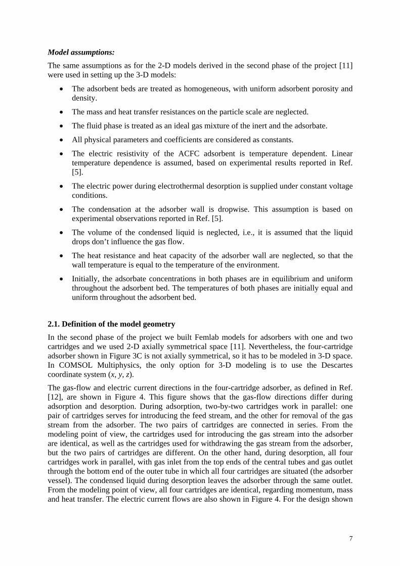
The gas-flow and electric current directions in the four-cartridge adsorber, as defined in Ref. [12], are shown in Figure 4. This figure shows that the gas-flow directions differ during adsorption and desorption. During adsorption, two-by-two cartridges work in parallel: one pair of cartridges serves for introducing the feed stream, and the other for removal of the gas stream from the adsorber. The two pairs of cartridges are connected in series. From the modeling point of view, the cartridges used for introducing the gas stream into the adsorber are identical, as well as the cartridges used for withdrawing the gas stream from the adsorber, but the two pairs of cartridges are different. On the other hand, during desorption, all four cartridges work in parallel, with gas inlet from the top ends of the central tubes and gas outlet through the bottom end of the outer tube in which all four cartridges are situated (the adsorber vessel). The condensed liquid during desorption leaves the adsorber through the same outlet. From the modeling point of view, all four cartridges are identical, regarding momentum, mass and heat transfer. The electric current flows are also shown in Figure 4. For the design shown
7
in this figure, all four cartridges are connected in series. From the modeling point of view, all four cartridges are different, regarding the electric current flow.
Figure 4. Four-cartridge adsorber [12]
In principle, the complete adsorber geometry with four cartridges should be used, in order to model the adsorber in which all four cartridges are different (e.g. because of different electric current flows through them). Nevertheless, 3-D models are very complex and very demanding regarding computer memory and computer time. For that reason, we explored two other options: to model a four-cartridge adsorber in which two cartridges can be considered as equal, and a four-cartridge adsorber in which all four cartridges are equal.
2.1.1. A 3-D model of the whole adsorber
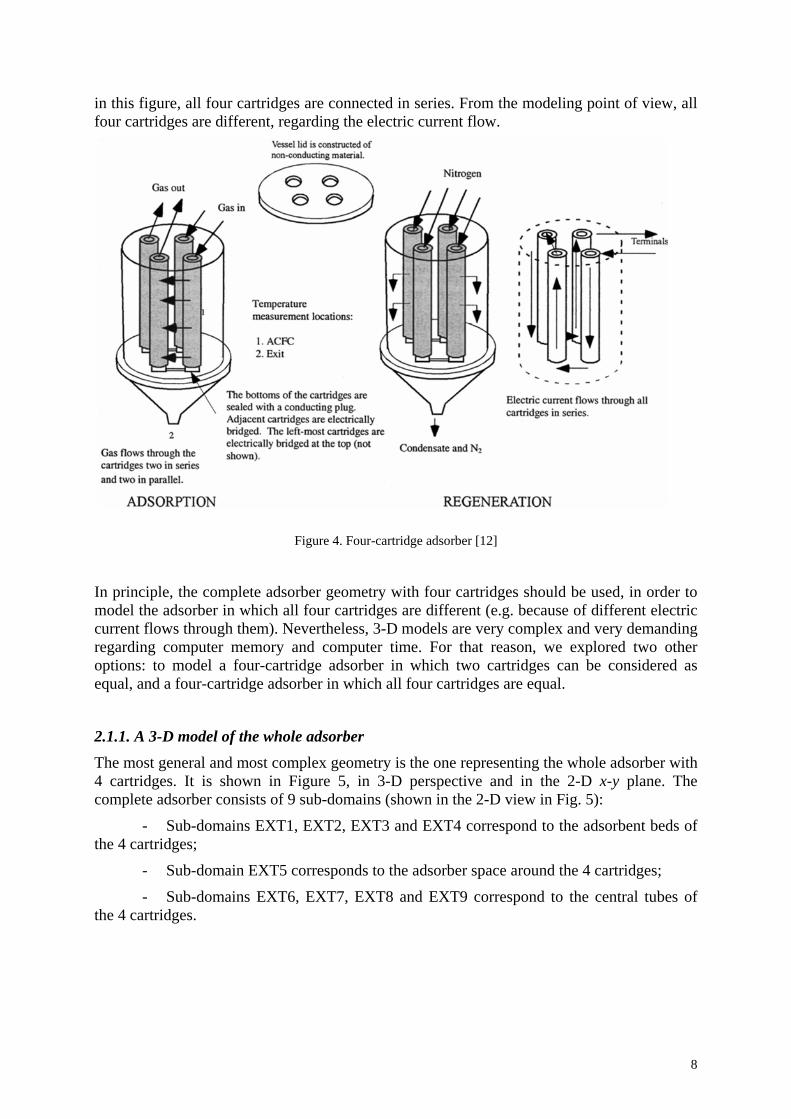
The most general and most complex geometry is the one representing the whole adsorber with 4 cartridges. It is shown in Figure 5, in 3-D perspective and in the 2-D x-y plane. The complete adsorber consists of 9 sub-domains (shown in the 2-D view in Fig. 5):
- Sub-domains EXT1, EXT2, EXT3 and EXT4 correspond to the adsorbent beds of the 4 cartridges;
- Sub-domain EXT5 corresponds to the adsorber space around the 4 cartridges;
- Sub-domains EXT6, EXT7, EXT8 and EXT9 correspond to the central tubes of the 4 cartridges.
8
In order to optimize computer memory usage and computer time consumption, we assumed that one quarter of the adsorbent would realistically represent the behavior of the system. Fig. 2 presents the geometry of the system, shown in isometric view along with x-y projection plane. One can notice three sub-domains:
E1 – the central, inlet tube, (one of four)
CO2 – the adsorbent bed, (one of four)
CO1 – the space between the cartridges (one quarter).
Mesh used for the finite element numerical simulation in FEMLAB is shown in Fig. 3. One quarter mesh consists of 141,922 elements, while the whole system would contain 570,249 elements.
Figure 5. Geometry definition for the whole four-cartridge adsorber: 3-D view (left) and 2-D x-y view (right)
If “coarser mesh” is chosen as a mesh parameter, with all other default parameter settings, the mesh corresponding to this geometry contains 24481 3-D elements.
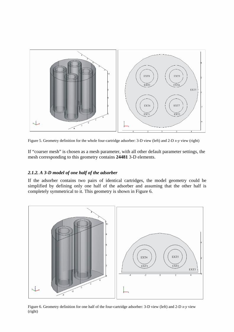
2.1.2. A 3-D model of one half of the adsorber If the adsorber contains two pairs of identical cartridges, the model geometry could be simplified by defining only one half of the adsorber and assuming that the other half is completely symmetrical to it. This geometry is shown in Figure 6.
9
Figure 6. Geometry definition for one half of the four-cartridge adsorber: 3-D view (left) and 2-D x-y view (right)
For this geometry, the number of sub-domains reduces to 5 (shown in the 2-D view in Fig. 6):
- Sub-domains EXT1 and EXT2 correspond to the adsorbent beds of the two cartridges;
- Sub-domain EXT3 corresponds to the space around the cartridges;
- Sub-domains EXT4 and EXT5 correspond to the central tubes of the two cartridges.
For “coarser mesh” setting, the mesh for this geometry consists of 12118 3-D elements.
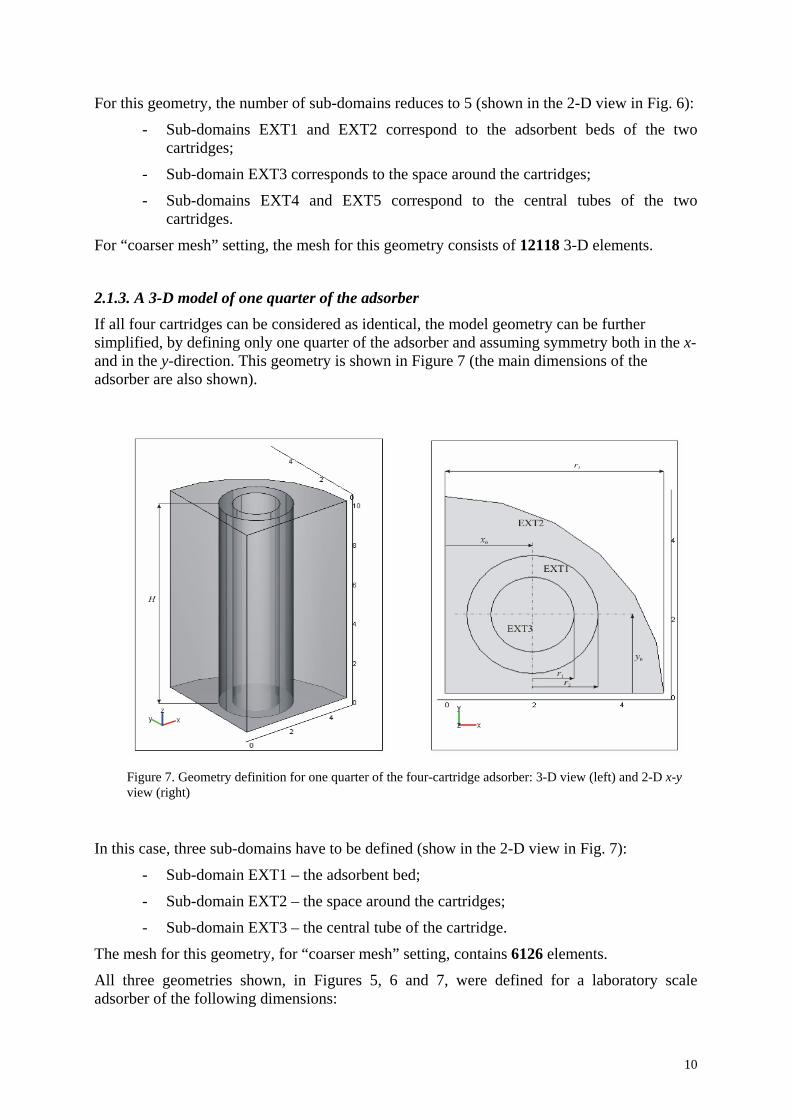
2.1.3. A 3-D model of one quarter of the adsorber If all four cartridges can be considered as identical, the model geometry can be further simplified, by defining only one quarter of the adsorber and assuming symmetry both in the x- and in the y-direction. This geometry is shown in Figure 7 (the main dimensions of the adsorber are also shown).
Figure 7. Geometry definition for one quarter of the four-cartridge adsorber: 3-D view (left) and 2-D x-y view (right)
In this case, three sub-domains have to be defined (show in the 2-D view in Fig. 7):
- Sub-domain EXT1 – the adsorbent bed;
- Sub-domain EXT2 – the space around the cartridges;
- Sub-domain EXT3 – the central tube of the cartridge.
The mesh for this geometry, for “coarser mesh” setting, contains 6126 elements.
All three geometries shown, in Figures 5, 6 and 7, were defined for a laboratory scale adsorber of the following dimensions:
10
- H=10 cm (height of the adsorber)
- r1=0.95 cm (radius of the central tubes)
- r2= 1.5 cm (outer radius of the adsorbent beds)
- r3=5 cm (radius of the adsorber vessel)
- x0=y0=2 cm (position of the cartridge center in the x and y directions)
2.2. The application modes used For modeling of the four-cartridge adsorber, the same built-in application modes are used, as for the one- or two-cartridge adsorbers (Ref. 11). For the most complex process – electrothermal desorption, in which simultaneous gas flow throw tubes and adsorbent beds, mass and heat transfer and heat generation by the Joule effect are coupled, seven application modes have to be incorporated in the COMSOL Multiphysics model:
1. Non-isothermal flow – for defining the momentum balances in the central tubes and outer space;
2. Brinkman equations – for defining the momentum balances for the adsorbent beds;
3. Convection and Conduction – for defining the heat balances for the gas phase;
4. Heat transfer by Conduction – for defining the heat balances for the solid phase;
5. Conductive Media DC – for defining heat generation by Joule effect;
6. Convection and Diffusion – for defining the mass balances for the gas phase;
7. Diffusion – for defining the mass balances for the solid phase.
The application modes are active in the sub-domains according to this scheme:
• Convection and Conduction and Convection and Diffusion are active in all sub-domains;
• Non-isothermal flow is active in sub-domains corresponding to the central tubes of the cartridges and the space around the cartridges;
• Brinkman equations, Heat transfer by Conduction, Conductive Media DC and Diffusion are active only in the sub-domains corresponding to the adsorbent beds.
2.3 The underlying equations In principle, the phenomena taking place in the four-cartridge TSA system are the same as in the one- and two-cartridge systems. Nevertheless, as a result of using 3-D Descartes instead of 2-D radial coordinate system, the model equations are not exactly the same. Although the model equations and their boundary conditions for different steps of the TSA process are somewhat different, as electrothermal desorption involves all phenomena and the corresponding application modes, here is an overview of the PDEs underlying the FEMLAB model for electrothermal desorption:
11
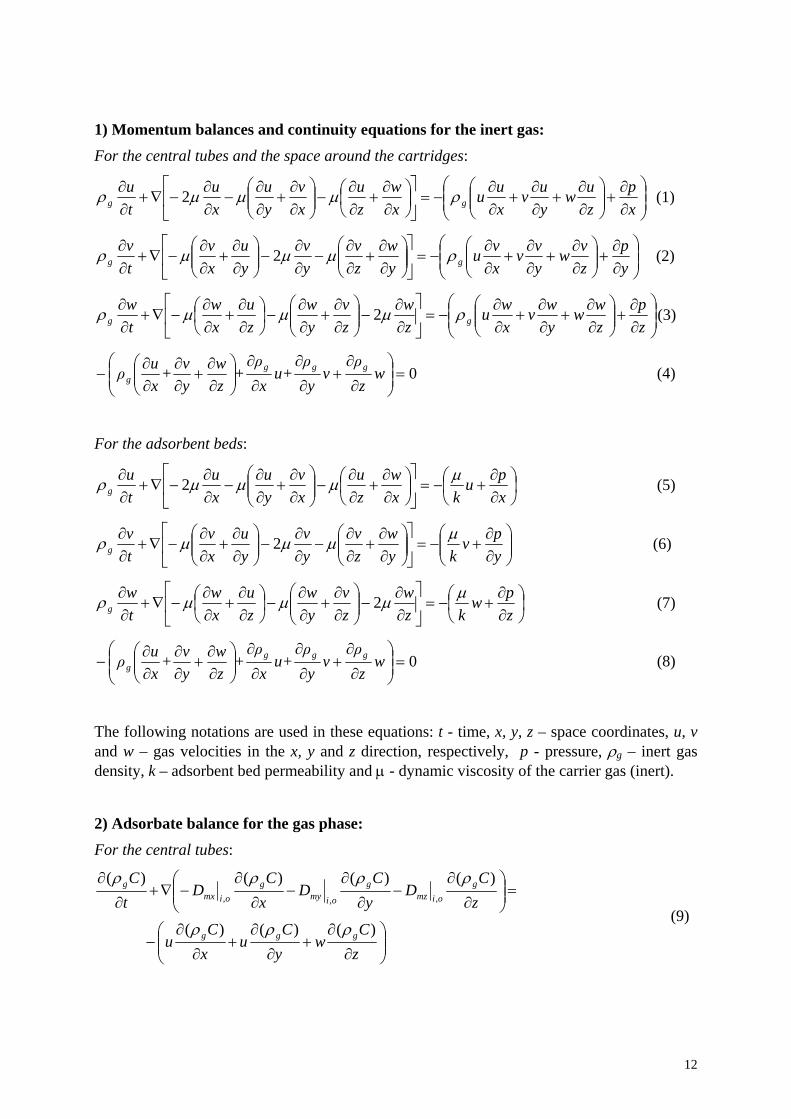
1) Momentum balances and continuity equations for the inert gas: For the central tubes and the space around the cartridges:
⎟⎟⎠
⎞⎜⎜⎝
⎛∂∂
+⎟⎟⎠
⎞⎜⎜⎝
⎛∂∂
+∂∂
+∂∂
−=⎥⎦
⎤⎢⎣
⎡⎟⎠⎞
⎜⎝⎛
∂∂
+∂∂
−⎟⎟⎠
⎞⎜⎜⎝
⎛∂∂
+∂∂
−∂∂
−∇+∂∂
xp
zuw
yuv
xuu
xw
zu
xv
yu
xu
tu
gg ρµµµρ 2 (1)
⎟⎟⎠
⎞⎜⎜⎝
⎛∂∂
+⎟⎟⎠
⎞⎜⎜⎝
⎛∂∂
+∂∂
+∂∂
−=⎥⎦
⎤⎢⎣
⎡⎟⎟⎠
⎞⎜⎜⎝
⎛∂∂
+∂∂
−∂∂
−⎟⎟⎠
⎞⎜⎜⎝
⎛∂∂
+∂∂
−∇+∂∂
yp
zvw
yvv
xvu
yw
zv
yv
yu
xv
tv
gg ρµµµρ 2 (2)
⎟⎟⎠
⎞⎜⎜⎝
⎛∂∂
+⎟⎟⎠
⎞⎜⎜⎝
⎛∂∂
+∂∂
+∂∂
−=⎥⎦
⎤⎢⎣
⎡∂∂
−⎟⎟⎠
⎞⎜⎜⎝
⎛∂∂
+∂∂
−⎟⎠⎞
⎜⎝⎛
∂∂
+∂∂
−∇+∂∂
zp
zww
ywv
xwu
zw
zv
yw
zu
xw
tw
gg ρµµµρ 2 (3)
0=⎟⎟⎠
⎞⎜⎜⎝
⎛∂
∂+
∂
∂
∂
∂⎟⎟⎠
⎞⎜⎜⎝
⎛∂∂
+∂∂
∂∂
− wzρ
vyρ
u+xρ
+zw
yv+
xuρ ggg
g (4)
For the adsorbent beds:
⎟⎠⎞
⎜⎝⎛
∂∂
+−=⎥⎦
⎤⎢⎣
⎡⎟⎠⎞
⎜⎝⎛
∂∂
+∂∂
−⎟⎟⎠
⎞⎜⎜⎝
⎛∂∂
+∂∂
−∂∂
−∇+∂∂
xpu
kxw
zu
xv
yu
xu
tu
gµµµµρ 2 (5)
⎟⎟⎠
⎞⎜⎜⎝
⎛∂∂
+−=⎥⎦
⎤⎢⎣
⎡⎟⎟⎠
⎞⎜⎜⎝
⎛∂∂
+∂∂
−∂∂
−⎟⎟⎠
⎞⎜⎜⎝
⎛∂∂
+∂∂
−∇+∂∂
ypv
kyw
zv
yv
yu
xv
tv
gµµµµρ 2 (6)
⎟⎠⎞
⎜⎝⎛
∂∂
+−=⎥⎦
⎤⎢⎣
⎡∂∂
−⎟⎟⎠
⎞⎜⎜⎝
⎛∂∂
+∂∂
−⎟⎠⎞
⎜⎝⎛
∂∂
+∂∂
−∇+∂∂
zpw
kzw
zv
yw
zu
xw
tw
gµµµµρ 2 (7)
0=⎟⎟⎠
⎞⎜⎜⎝
⎛∂
∂+
∂
∂
∂
∂⎟⎟⎠
⎞⎜⎜⎝
⎛∂∂
+∂∂
∂∂
− wzρ
vyρ
u+xρ
+zw
yv+
xuρ ggg
g (8)
The following notations are used in these equations: t - time, x, y, z – space coordinates, u, v and w – gas velocities in the x, y and z direction, respectively, p - pressure, ρg – inert gas density, k – adsorbent bed permeability and µ - dynamic viscosity of the carrier gas (inert).
2) Adsorbate balance for the gas phase: For the central tubes:
⎟⎟⎠
⎞⎜⎜⎝
⎛∂
∂+
∂
∂+
∂
∂−
=⎟⎟⎠
⎞⎜⎜⎝
⎛∂
∂−
∂
∂−
∂
∂−∇+
∂
∂
zC
wyC
uxC
u
zC
DyC
DxC
DtC
ggg
goimz
g
oimyg
oimxg
)()()(
)()()()(,,,
ρρρ
ρρρρ
(9)
12
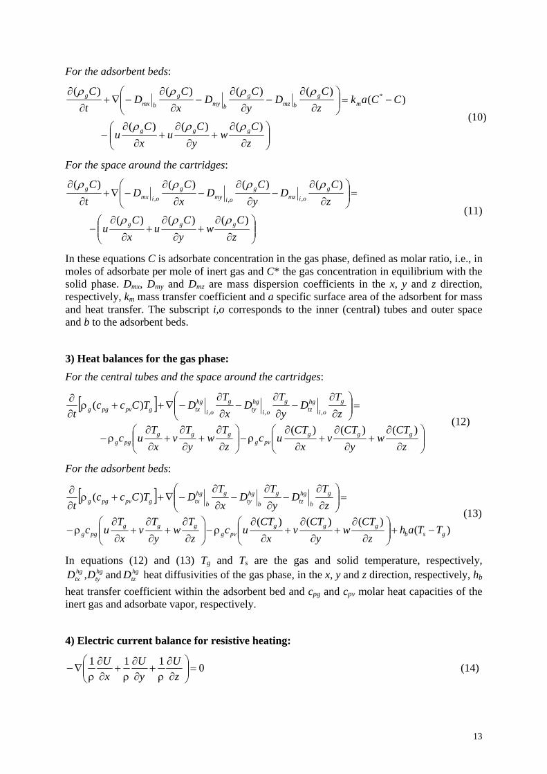
For the adsorbent beds:
⎟⎟⎠
⎞⎜⎜⎝
⎛∂
∂+
∂∂
+∂
∂−
−=⎟⎟⎠
⎞⎜⎜⎝
⎛∂
∂−
∂∂
−∂
∂−∇+
∂∂
zC
wyC
uxC
u
CCakzC
DyC
DxC
DtC
ggg
mg
bmzg
bmyg
bmxg
)()()(
)()()()()( *
ρρρ
ρρρρ
(10)
For the space around the cartridges:
⎟⎟⎠
⎞⎜⎜⎝
⎛∂
∂+
∂
∂+
∂
∂−
=⎟⎟⎠
⎞⎜⎜⎝
⎛∂
∂−
∂
∂−
∂
∂−∇+
∂
∂
zC
wyC
uxC
u
zC
DyC
DxC
DtC
ggg
goimz
g
oimyg
oimxg
)()()(
)()()()(,,,
ρρρ
ρρρρ
(11)
In these equations C is adsorbate concentration in the gas phase, defined as molar ratio, i.e., in moles of adsorbate per mole of inert gas and C* the gas concentration in equilibrium with the solid phase. Dmx, Dmy and Dmz are mass dispersion coefficients in the x, y and z direction, respectively, km mass transfer coefficient and a specific surface area of the adsorbent for mass and heat transfer. The subscript i,o corresponds to the inner (central) tubes and outer space and b to the adsorbent beds.
3) Heat balances for the gas phase: For the central tubes and the space around the cartridges:
[ ]
⎟⎟⎠
⎞⎜⎜⎝
⎛∂
∂+
∂
∂+
∂
∂ρ−⎟⎟
⎠
⎞⎜⎜⎝
⎛∂
∂+
∂
∂+
∂
∂ρ−
=⎟⎟⎠
⎞⎜⎜⎝
⎛∂
∂−
∂
∂−
∂
∂−∇++ρ
∂∂
zCT
wy
CTv
xCT
ucz
Tw
yT
vxT
uc
zT
DyT
DxT
DTCcct
gggpvg
gggpgg
g
oi
hgtz
g
oi
hgty
g
oi
hgtxgpvpgg
)()()(
)(,,,
(12)
For the adsorbent beds:
[ ]
)()()()(
)(
gsbggg
pvgggg
pgg
g
b
hgtz
g
b
hgty
g
b
hgtxgpvpgg
TTahz
CTw
yCT
vx
CTuc
zT
wyT
vx
Tuc
zT
DyT
DxT
DTCcct
−+⎟⎟⎠
⎞⎜⎜⎝
⎛∂
∂+
∂
∂+
∂
∂ρ−⎟⎟
⎠
⎞⎜⎜⎝
⎛∂
∂+
∂
∂+
∂
∂ρ−
=⎟⎟⎠
⎞⎜⎜⎝
⎛∂
∂−
∂
∂−
∂
∂−∇++ρ
∂∂
(13)
In equations (12) and (13) Tg and Ts are the gas and solid temperature, respectively, heat diffusivities of the gas phase, in the x, y and z direction, respectively, hhg
tzhgty
hgtx DDD and, b
heat transfer coefficient within the adsorbent bed and cpg and cpv molar heat capacities of the inert gas and adsorbate vapor, respectively.
4) Electric current balance for resistive heating:
0111=⎟⎟
⎠
⎞⎜⎜⎝
⎛∂∂
ρ+
∂∂
ρ+
∂∂
ρ∇−
zU
yU
xU (14)
13
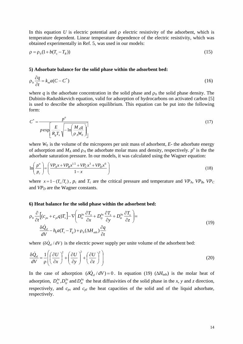
In this equation U is electric potential and ρ electric resistivity of the adsorbent, which is temperature dependent. Linear temperature dependence of the electric resistivity, which was obtained experimentally in Ref. 5, was used in our models:
))(1(0 Rs TTb −+ρ=ρ (15)
5) Adsorbate balance for the solid phase within the adsorbent bed:
)( *CCaktq
mb −=∂∂
ρ (16)
where q is the adsorbate concentration in the solid phase and ρb the solid phase density. The Dubinin-Radushkevich equation, valid for adsorption of hydrocarbons on activated carbon [5] is used to describe the adsorption equilibrium. This equation can be put into the following form:
⎥⎥⎦
⎤
⎢⎢⎣
⎡⎟⎟⎠
⎞⎜⎜⎝
⎛ρ
−
=
0
*
lnexpW
qMTR
Ep
pC
A
A
sg
o
(17)
where W0 is the volume of the micropores per unit mass of adsorbent, E- the adsorbate energy of adsorption and MA and ρA the adsorbate molar mass and density, respectively. po is the the adsorbate saturation pressure. In our models, it was calculated using the Wagner equation:
⎟⎟⎠
⎞⎜⎜⎝
⎛
−+++
=⎟⎟⎠
⎞⎜⎜⎝
⎛
xxVPxVPxVPxVP
pp DCBA
c
o
1ln
635.1
(18)
where )(1 cs TTx −= , pc and Tc are the critical pressure and temperature and VPA, VPB, VPC and VPD are the Wagner constants.
6) Heat balance for the solid phase within the adsorbent bed:
[ ]
tqHTTah
dVQ
zTD
yTD
xTDTqcc
t
adsbgsbel
shstz
shsty
shstxsplpsb
∂∂
∆ρ+−−δ
=⎟⎟⎠
⎞⎜⎜⎝
⎛∂∂
+∂∂
+∂∂
∇−+∂∂
ρ
)()(
)(
& (19)
where is the electric power supply per unite volume of the adsorbent bed: )/( dVQel&δ
⎟⎟
⎠
⎞
⎜⎜
⎝
⎛⎟⎠⎞
⎜⎝⎛∂∂
+⎟⎟⎠
⎞⎜⎜⎝
⎛∂∂
+⎟⎠⎞
⎜⎝⎛∂∂
ρ=
δ 2221zU
yU
xU
dVQel&
(20)
In the case of adsorption . In equation (19) (∆H0)/( =dVQel&δ ads) is the molar heat of
adsorption, the heat diffusivities of the solid phase in the x, y and z direction, respectively, and c
hstz
hsty
hstx DDD and,
ps and cpl the heat capacities of the solid and of the liquid adsorbate, respectively.
14
Boundary conditions: The boundary conditions listed bellow correspond to the gas flow dirrections defined for the desorption step in Figure 4, and for one quarter of the four-cartridge adsorber.
- For the bottom surface of the central tube:
0,0
,0,0,0:)()(,0
,,
21
20
20
=∂∂
−=∂∂
−
===<−+−=
zCD
zT
D
wvuryyxxz
oimzg
oi
hgtz
(21)
- For the top surface of the central tube:
ingingg
CCTTr
GwvuryyxxHz ==πρ
===<−+−= ,,,0,0:)()(, 21
21
20
20 (22)
- For the cylindrical surface of the central tube:
0),(
),)(1()(
)(
))(1()()(
)()(
,,,:),0(,)()(
1
*1
,,
1
,,
,2
12
02
0
=−=∂∂
−∂∂
−
−ε−+⎟⎟⎠
⎞⎜⎜⎝
⎛++
∂∂
−∂∂
−
=⎟⎟⎠
⎞⎜⎜⎝
⎛++
∂∂
−∂∂
−
−ε−+⎟⎟⎠
⎞⎜⎜⎝
⎛++ρ+
∂
∂−
∂
∂−
=⎟⎟⎠
⎞⎜⎜⎝
⎛++ρ+
∂
∂−
∂
∂−
====∈=−+−
JTThyTD
xTD
CCkCvuyCD
xCD
CvuyCD
xCD
TThvuTCccy
TD
xT
D
vuTCccy
TD
xT
D
wwvvuuppHzryyxx
sgsshs
tyshs
tx
bmb
bmxbmx
itoimyoimx
gsbsb
gpvpggg
b
hgty
g
b
hgtx
itgpvpgg
g
oi
hgty
g
oi
hgtx
bitbitbitbit
(23)
- For the bottom surface of the adsorbent bed:
0,0,0,0
,0,0,0:)()(,0 22
20
20
21
=∂∂
−==∂∂
−=∂∂
−
===<−+−<=
zTDU
zCD
zT
D
wvuryyxxrz
shstzbmz
g
b
hgtz
(24)
- For the top surface of the adsorbent bed:
0,,0,0
,0,0,0:)()(,
0
22
20
20
21
=∂∂
−==∂∂
−=∂∂
−
===<−+−<=
zTDUU
zCD
zT
D
wvuryyxxrHz
shstzbmz
g
b
hgtz
(25)
15
- For the outer cylindrical surface of the adsorbent bed:
0),(
),)(1()(
)(
))(1()()(
)()(
,,,:),0(,)()(
1
*2,,
2,,
,2
22
02
0
=−=∂∂
−∂∂
−
−ε−+⎟⎟⎠
⎞⎜⎜⎝
⎛++
∂∂
−∂∂
−
=⎟⎟⎠
⎞⎜⎜⎝
⎛++
∂∂
−∂∂
−
−ε−+⎟⎟⎠
⎞⎜⎜⎝
⎛++ρ+
∂
∂−
∂
∂−
=⎟⎟⎠
⎞⎜⎜⎝
⎛++ρ+
∂
∂−
∂
∂−
====∈=−+−
JTThyTD
xTD
CCkCvuyCD
xCD
CvuyCD
xCD
TThvuTCccy
TD
xT
D
vuTCccy
TD
xT
D
wwvvuuppHzryyxx
sgsshs
tyshs
tx
bmot
oimroimr
bbmybmx
gsbsot
gpvpggg
oi
hgty
g
oi
hgtx
bgpvpgg
g
b
hgty
g
b
hgtx
otbotbotbotb
(26)
- For the bottom surface of the space around the cartridges:
0,0,
:),0(),,0()()(,0
,,
332
3222
22
02
0
=∂∂
−=∂∂
−=
∈∈∩<+∩>−+−=
zCD
zT
Dpp
ryrxryxryxxxz
oimzg
oi
hgtzaot
(27)
- For the top surface of the space around the cartridges:
0,0,0,0,0
:),0(),,0()()(,
,,
332
3222
22
02
0
=∂∂
−=∂∂
−===
∈∈∩<+∩>−+−=
zCD
zT
Dwvu
ryrxryxryxxxHz
oimzg
oi
hgtz
(28)
- For the adsorber wall:
)(,0
,0,0,0:),0(,
,,,,
23
22
agwgg
oi
hgty
g
oi
hgtxoimyoimx TTh
yT
DxT
DyCD
xCD
wvuHzryx
−=∂∂
−∂∂
−=∂∂
−∂∂
−
===∈=+ (29)
For the case of desorption accompanied with condensation, the boundary condition (29) has to be changed in the following way [11]:
)()(),(
,0,0,0:),0(,
,,,,
23
22
agwgcondoimyoimxg
oi
hgty
g
oi
hgtxwsat TThH
yCD
xCD
yT
Dx
TDTCC
wvuHzryx
−∆⎟⎟⎠
⎞⎜⎜⎝
⎛∂∂
+∂∂
−=∂
∂−
∂
∂−=
===∈=+(29a)
In equations (21-29), r1, r2, r3, x0, y0 and H are the adsorber dimensions which have been defined in Figure 7. G is the molar flow-rate of the gas inert, U0 – the supply voltage (0 for adsorption) and εb - bed porosity. The subscript in denotes inlet, it the inner (central) tube, ot the space around the cartridges, a the ambient and w the adsorber wall. (∆Hcond) is the molar
16
heat of condensation and Csat(Tw) the saturation concentration corresponding to the wall temperature Tw , which was calculated using the Wagner equation.
Although the heat and mass transfer coefficients, dispersion coefficients, etc., can be defined as functions of the dependent variables (velocities, concentrations, temperatures), in our current models constant values were used in order to reduce the convergence problems. The adsorption isotherm relation (q=f(C, Ts)) and the temperature dependence of the electric resistivity were included in the models (equations (17) and (15), respectively).
3. Solution of the models The Models of the four-cartridge adsorber were developed and solved using a personal computer with AMD ATHLON™ 64 3000+ processor and with 4 GB RAM.
Our 3-D models are very complex, regarding both the geometry and the number of application modes used. Even with a “coarser” mesh, the number of degrees of freedom obtained is very high. This number was so high, that the models for the whole and for one half of the four-cartridge adsorber (Figs. 5 and 6) could not be solved at all, owing to the lack of computer memory. Because of that, we focused our efforts on solving the model of a quarter of the adsorber, assuming model symmetry in the x and y directions (Fig. 7).
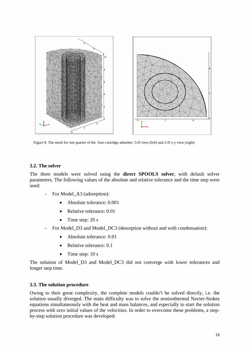
3.1. The mesh parameters In order to reduce the memory requirements, the following mesh parameters were used:
- Predefined mesh sizes: “coarser”
- Maximum element size scaling factor: 1.9
- Element growth rate: 1.7
With these mesh parameters the following mesh statistics was obtained:
- Number of mesh elements: 2237
- Minimum element quality: 0.2578.
The mesh with these characteristics is presented in Figure 8.
17
.2. The solver ls were solved using the direct SPOOLS solver, with default solver
- For Model_A3 (adsorption):
001
- For Model_D3 and Model_DC3 (desorption without and with condensation):
The solution of Model_D3 and Model_DC3 did not converge with lower tolerances and
.3. The solution procedure ity, the complete models couldn’t be solved directly, i.e. the
Figure 8. The mesh for one quarter of the four-cartridge adsorber: 3-D view (left) and 2-D x-y view (right)
3The three modeparameters. The following values of the absolute and relative tolerance and the time step were used:
• Absolute tolerance: 0.
• Relative tolerance: 0.01
• Time step: 20 s
• Absolute tolerance: 0.01
• Relative tolerance: 0.1
• Time step: 10 s
longer step time.
3Owing to their great complexsolution usually diverged. The main difficulty was to solve the nonisothermal Navier-Stokes equations simultaneously with the heat and mass balances, and especially to start the solution process with zero initial values of the velocities. In order to overcome these problems, a step-by-step solution procedure was developed:
18
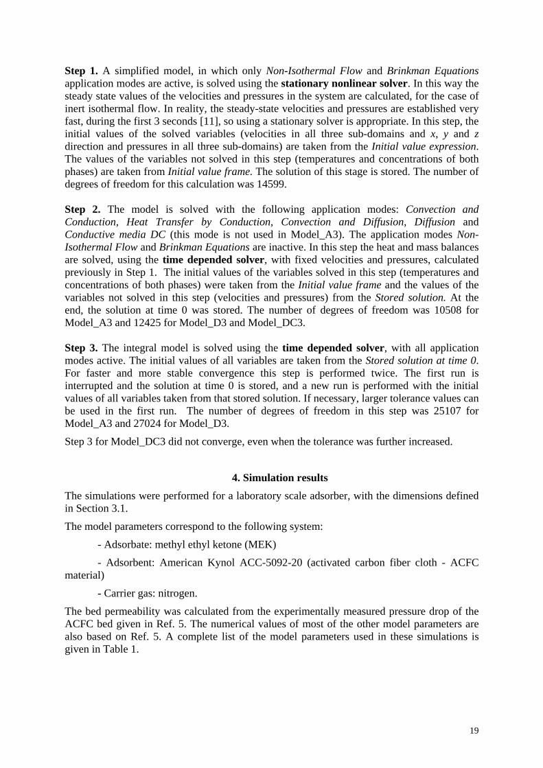
Step 1. A simplified model, in which only Non-Isothermal Flow and Brinkman Equations application modes are active, is solved using the stationary nonlinear solver. In this way the
vection and Diffusion, Diffusion and
n from the Stored solution at time 0.
he simulations were performed for a laboratory scale adsorber, with the dimensions defined in Section 3.1.
ate: methyl ethyl ketone (MEK)
ated carbon fiber cloth - ACFC
ermeability was calculated from the experimentally measured pressure drop of the e numerical values of most of the other model parameters are
steady state values of the velocities and pressures in the system are calculated, for the case of inert isothermal flow. In reality, the steady-state velocities and pressures are established very fast, during the first 3 seconds [11], so using a stationary solver is appropriate. In this step, the initial values of the solved variables (velocities in all three sub-domains and x, y and z direction and pressures in all three sub-domains) are taken from the Initial value expression. The values of the variables not solved in this step (temperatures and concentrations of both phases) are taken from Initial value frame. The solution of this stage is stored. The number of degrees of freedom for this calculation was 14599. Step 2. The model is solved with the following application modes: Convection and
onduction, Heat Transfer by Conduction, ConCConductive media DC (this mode is not used in Model_A3). The application modes Non-Isothermal Flow and Brinkman Equations are inactive. In this step the heat and mass balances are solved, using the time depended solver, with fixed velocities and pressures, calculated previously in Step 1. The initial values of the variables solved in this step (temperatures and concentrations of both phases) were taken from the Initial value frame and the values of the variables not solved in this step (velocities and pressures) from the Stored solution. At the end, the solution at time 0 was stored. The number of degrees of freedom was 10508 for Model_A3 and 12425 for Model_D3 and Model_DC3. Step 3. The integral model is solved using the time depended solver, with all application
odes active. The initial values of all variables are takemFor faster and more stable convergence this step is performed twice. The first run is interrupted and the solution at time 0 is stored, and a new run is performed with the initial values of all variables taken from that stored solution. If necessary, larger tolerance values can be used in the first run. The number of degrees of freedom in this step was 25107 for Model_A3 and 27024 for Model_D3.
Step 3 for Model_DC3 did not converge, even when the tolerance was further increased.
4. Simulation results
T
The model parameters correspond to the following system:
- Adsorb
- Adsorbent: American Kynol ACC-5092-20 (activmaterial)
- Carrier gas: nitrogen.
The bed pACFC bed given in Ref. 5. Thalso based on Ref. 5. A complete list of the model parameters used in these simulations is given in Table 1.
19
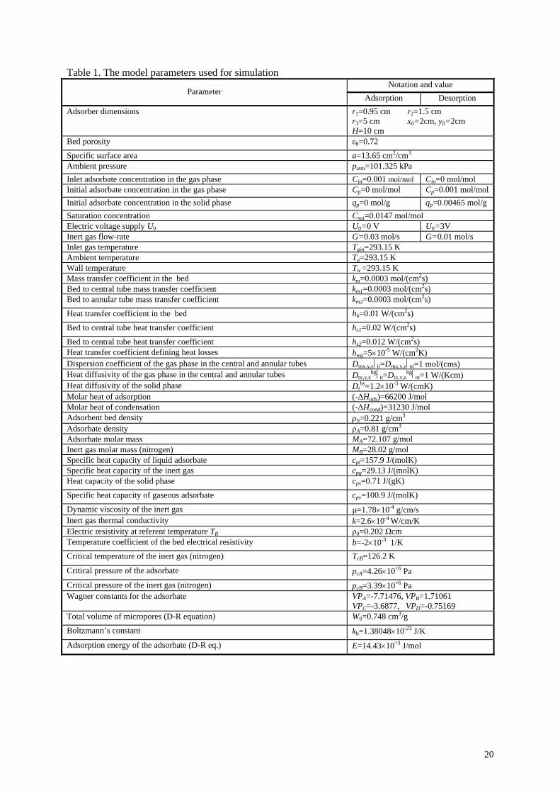
Table 1. The model parameters used for simulation Notation and value
Parameter Adsorption Desorption
r1=0.95 cm r =1.5 cm r3=5 cm m H=
Adsorber dimensions 2 x0=2cm, y0=2c
10 cm Bed porosity εb=0.72
Specific surface area a=13.65 cm2/cm3
Ambient pressure patm=101.325 kPa Inlet adsorbate concentration in the gas phase 1 mol/mol Cin=0 mol/mol Cin=0.00Initial adsorbate concentration in the gas phase Cp=0.001 mol/mol Cp=0 mol/mol Initial adsorbate concentration in the solid phase qp=0.00465 mol/g qp=0 mol/g Saturation concentration Csat=0.0147 mol/mol Electric voltage supply U0 U0=0 V U0=3V Inert gas flow-rate G=0.03 mol/s G=0.01 mol/s Inlet gas temperature Tgin=293.15 K Ambient temperature Ta=293.15 K Wall temperature Tw = 5 K 293.1Mass transfer coefficient in the bed (cm2skm /=0.0003 mol ) Bed to central tube mass transfer coefficient /(cm2s) k =0.0003 molm1Bed to annular tube mass transfer coefficient l/(cm2s) k =0.0003 mom2
Heat transfer coefficient in the bed hb=0.01 W/(cm2s)
Bed to central tube heat transfer coefficient hs1=0.02 W/(cm2s)
Bed to central tube heat transfer coefficient hs2=0.012 W/(cm2s) Heat transfer coefficient defining heat losses K) hwg=5×10⁻⁵ W/(cm2
Dispersion coefficient of the gas phase in the central and annular tubes mol/(cms) Dmx,y,z⎜it=Dmx,y,z⎜ot=1Heat diffusivity of the gas phase in the central and annular tubes 1 W/(Kcm) Dtx,y,z
hg⎜it=Dtx,y,zhg⎜ot=
Heat diffusivity of the solid phase Dths -3=1.2×10 W/(cmK)
Molar heat of adsorption (-∆ adsH )=66 J/mol 200Molar heat of condensation (-∆H ) 23cond =31 0 J/mol Adsorbent bed density ρb=0.221 g/cm3
Adsorbate density ρA=0.81 g/cm3
Adsorbate molar mass MA=72.107 g/mol Inert gas molar mass (nitrogen) MB=28.02 g/mol Specific heat capacity of liquid adsorbate K) c =157.9 J/(mpl olSpecific heat capacity of the inert gas cpg=29.13 J/(molK)Heat capacity of the solid phase cps=0.71 J/(gK)
Specific heat capacity of gaseous adsorbate cpv=100.9 J/(molK)
Dynamic viscosity of the inert gas µ=1.78×10⁻⁴ g/cm/s Inert gas thermal conductivity k=2.6×10⁻⁴ W/cm/K Electric resistivity at referent temperature TR ρ0=0.202 Ωcm Temperature coefficient of the bed electrical resistivity b=-2×10⁻³ 1/K Critical temperature of the inert gas (nitrogen) TcB=126.2 K
Critical pressure of the adsorbate pcA=4.26×10+6 Pa Critical pressure of the inert gas (nitrogen) pcB=3.39×10+6 Pa Wagner constants for the adsorbate VPA=-7.71476, VPB=1.71061
D=-0.75169 VPC=-3.6877, VPTotal volume of micropores (D-R equation) W0=0.748 cm /g3
Boltzmann’s constant kb=1.38048×10⁻²³ J/K
Adsorption energy of the adsorbate (D-R eq.) E=14.43×10+3 J/mol
20

COMSOL Multiphysics offers a large number of options for graphical representation of the
ds in
- temperature fields in
For all thr se results are shown in
lectrothermal desorption process, were
alculation of the amount of the condensed liquid:
m the gas concentration gradient at the
simulated results. The following results were chosen for presentation in this report:
- Velocity field in the adsorber;
- Gas and solid concentration fielthe adsorber;
Gas and solid the adsorber.
ee models, thethe form of 3-D slice plots, corresponding to 3 different times. The arrows, showing the direction of the gas flow are also shown in these 3-D plots. Also, 2-D plots are given, corresponding to two cross-sections of the adsorber, one corresponding to x=y, and the other to z=H/2 (planes A and B in Figure 9). Time profiles, in 1-D diagrams, corresponding to 5 points in the adsorber, also defined in Figure 9, are alsointersection of planes A and B, two of them within the adsorbent bed, two in the space around the cartridges and one on the axes of the central tube.
Two additional parameters, very important for the e
Figure 9. Definition of the planes and points used for 2-D and 1-D presentation
given. These points lie at the
calculated and presented: the amount of the condensed liquid and the used electric energy.
C
The flux of the condensed liquid is calculated froadsorber wall:
23
22,,
),,,( tzyxJryx
oimyoimxcond yCD
xCD
=+∂∂
−∂∂
−= (30)
It should be noticed that, owing to the 3-D geometry, this flux is a function of all three
Hzryx
02
322
(31)
The total amount of the condensed liquid is obtained by integrating the condensation rate over
cond
dttLcondcond0
)(& (32)
τcond is the total time of condensation.
coordinates and time. The condensation rate is calculated by integration of the flux over the whole surface of the adsorber wall, and is a function of time only:
∫∫= condcond dzdydxtzyxJtL ),,,(4)(&
≤≤=+
time:
=L ∫τ
21
Calculation of the used electric energy:
y is equal to the Joule heat produced in the adsorbent
dsorbent bed
It is assumed that the used electric energmaterial. This energy per unit volume and unit time is defined by equation (20).
The used electric power per cartridge is obtained by integration over the avolume:
∫∫∫≤≤
<−+−<⎟⎟
⎠
⎞
⎜⎜
⎝
⎛⎟⎠⎞
⎜⎝⎛∂∂
+⎟⎟⎠
⎞⎜⎜⎝
⎛∂∂
+⎟⎠⎞
⎜⎝⎛∂∂
−+=
Hzryyxxr Rs
el dzdydxzU
yU
xU
TTbtQ
0)()(
222
022
20
20
21
))(1(1)(
ρ& (33)
and the total used energy during desorption, by integration over time and multiplying by 4:
∫τ
elel0
4)
τdes is the total desorption time.
.1. Simulation of adsorption
s performed using Model_A3. In order to reduce the memory
Velocity distribution
he velocity during adsorption is practically not
=des
dttQQ )(& (3
4
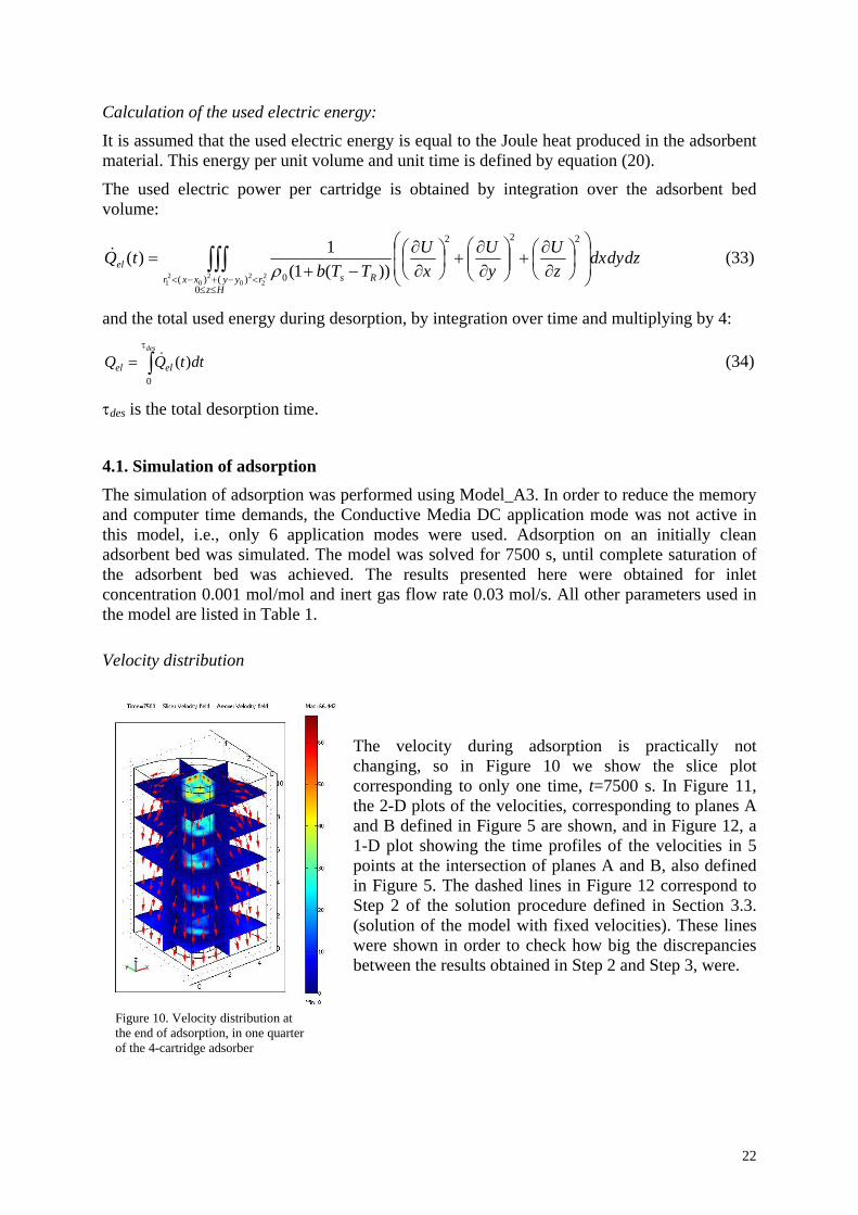
The simulation of adsorption waand computer time demands, the Conductive Media DC application mode was not active in this model, i.e., only 6 application modes were used. Adsorption on an initially clean adsorbent bed was simulated. The model was solved for 7500 s, until complete saturation of the adsorbent bed was achieved. The results presented here were obtained for inlet concentration 0.001 mol/mol and inert gas flow rate 0.03 mol/s. All other parameters used in the model are listed in Table 1.
Figure 10. Velocity distribution at the end of adsorption, in one quarter of the 4-cartridge adsorber
Tchanging, so in Figure 10 we show the slice plot corresponding to only one time, t=7500 s. In Figure 11, the 2-D plots of the velocities, corresponding to planes A and B defined in Figure 5 are shown, and in Figure 12, a 1-D plot showing the time profiles of the velocities in 5 points at the intersection of planes A and B, also defined in Figure 5. The dashed lines in Figure 12 correspond to Step 2 of the solution procedure defined in Section 3.3. (solution of the model with fixed velocities). These lines were shown in order to check how big the discrepancies between the results obtained in Step 2 and Step 3, were.
22
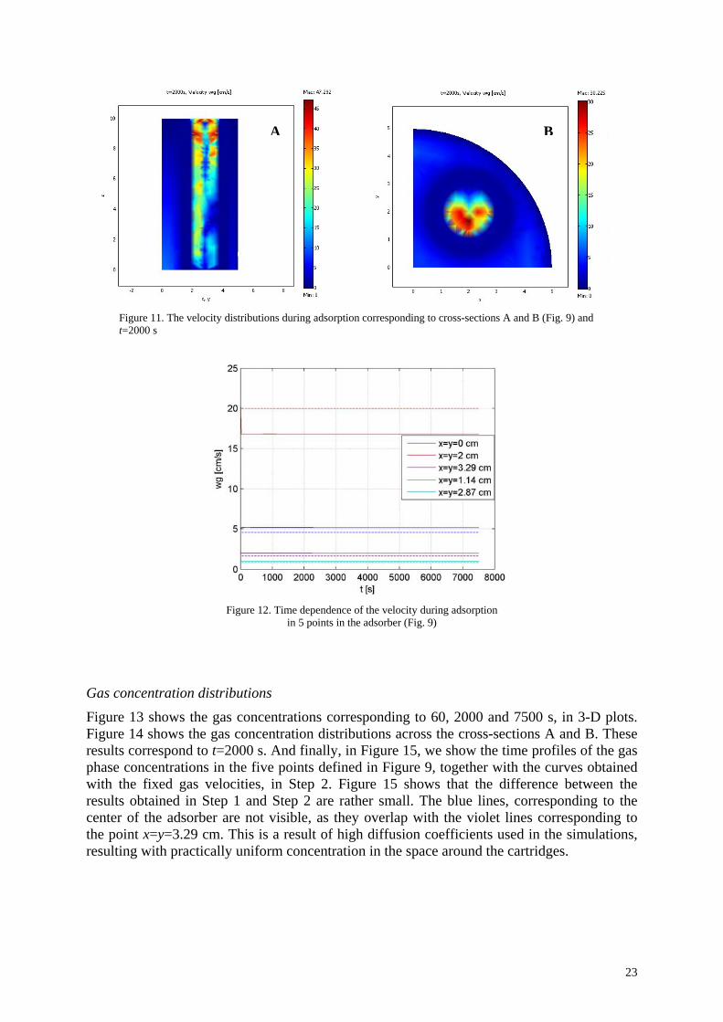
A B
Figure 11. The velocity distributions during adsorption corresponding to cross-sections A and B (Fig. 9) and t=2000 s
Figure 12. Time dependence of the velocity during adsorption
in 5 points in the adsorber (Fig. 9)
as concentration distributions
trations corresponding to 60, 2000 and 7500 s, in 3-D plots.
G
Figure 13 shows the gas concenFigure 14 shows the gas concentration distributions across the cross-sections A and B. These results correspond to t=2000 s. And finally, in Figure 15, we show the time profiles of the gas phase concentrations in the five points defined in Figure 9, together with the curves obtained with the fixed gas velocities, in Step 2. Figure 15 shows that the difference between the results obtained in Step 1 and Step 2 are rather small. The blue lines, corresponding to the center of the adsorber are not visible, as they overlap with the violet lines corresponding to the point x=y=3.29 cm. This is a result of high diffusion coefficients used in the simulations, resulting with practically uniform concentration in the space around the cartridges.
23
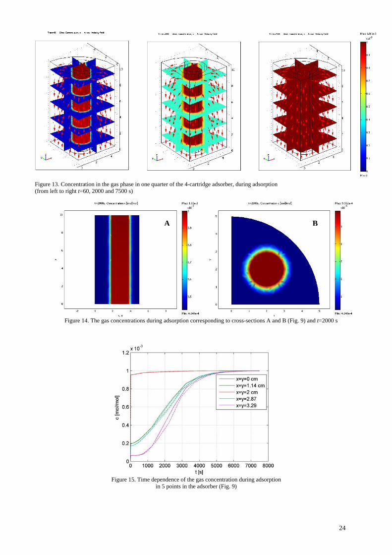
Figure 13. Concentration in the gas phase in one quarter of the 4-cartridge adsorber, during adsorption (from left to right t=60, 2000 and 7500 s)
A B
Figure 14. The gas concentrations during adsorption corresponding to cross-sections A and B (Fig. 9) and t=2000 s
Figure 15. Time dependence of the gas concentration during adsorption
in 5 points in the adsorber (Fig. 9)
24
Solid concentration distributions
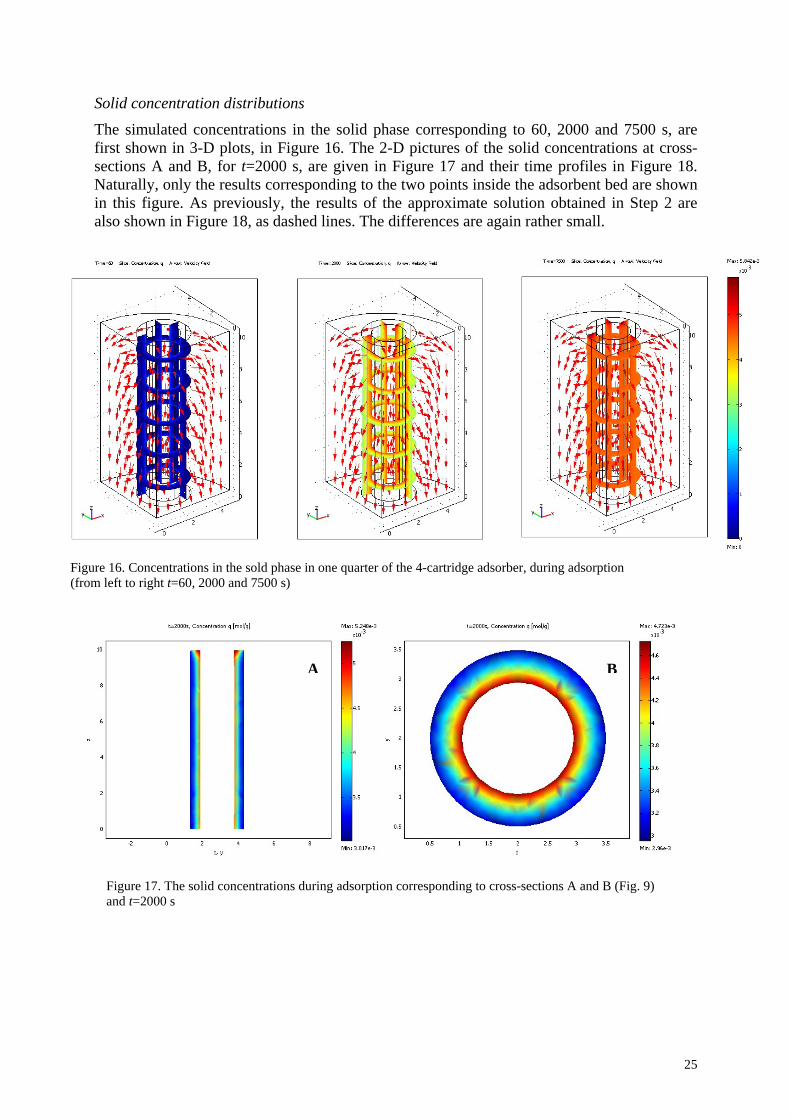
the solid phase corresponding to 60, 2000 and 7500 s, are The simulated concentrations in first shown in 3-D plots, in Figure 16. The 2-D pictures of the solid concentrations at cross-sections A and B, for t=2000 s, are given in Figure 17 and their time profiles in Figure 18. Naturally, only the results corresponding to the two points inside the adsorbent bed are shown in this figure. As previously, the results of the approximate solution obtained in Step 2 are also shown in Figure 18, as dashed lines. The differences are again rather small.
Figure 16. Concentrations in the sold phase in one quarter of the 4-cartridge adsorber, during adsorption (fro left to right t=60, 2000 and 7500 s) m
A B
Figure 17. The solid concentrations during adsorption corresponding to cross-sections A and B (Fig. 9) and t=2000 s
25
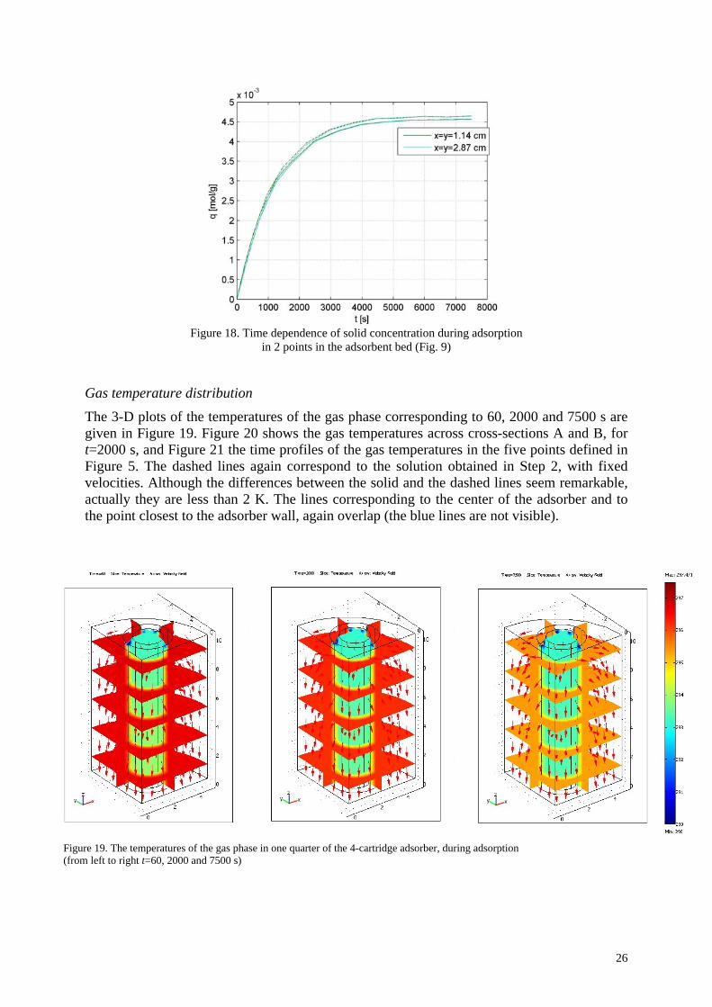
Figure 18. Time dependence of solid concentration during adsorption
in 2 points in the adsorbent bed (Fig. 9)
Gas temperature distribution
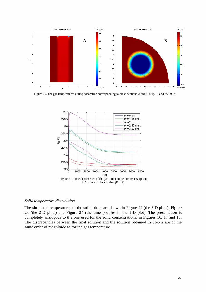
The 3-D plots of the temperatures of the gas phase corresponding to 60, 2000 and 7500 s are given in Figure 19. Figure 20 shows the gas temperatures across cross-sections A and B, for t=2000 s, and Figure 21 the time profiles of the gas temperatures in the five points defined in Figure 5. The dashed lines again correspond to the solution obtained in Step 2, with fixed velocities. Although the differences between the solid and the dashed lines seem remarkable, actually they are less than 2 K. The lines corresponding to the center of the adsorber and to the point closest to the adsorber wall, again overlap (the blue lines are not visible).
Figure 19. The temperatures of the gas phase in one quarter of the 4-cartridge adsorber, during adsorption (from left to right t=60, 2000 and 7500 s)
26
BA
Figure 20. The gas temperatures during adsorption corresponding to cross-sections A and B (Fig. 9) and t=2000 s
Figure 21. Time dependence of the gas temperature during adsorption
in 5 points in the adsorber (Fig. 9)
Solid temperature distribution
The simulated temperatures of the solid phase are shown in Figure 22 (the 3-D plots), Figure 23 (the 2-D plots) and Figure 24 (the time profiles in the 1-D plot). The presentation is completely analogous to the one used for the solid concentrations, in Figures 16, 17 and 18. The discrepancies between the final solution and the solution obtained in Step 2 are of the same order of magnitude as for the gas temperature.
27
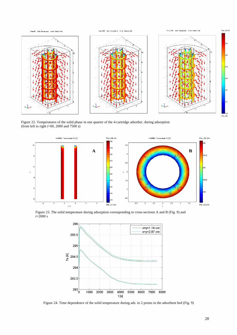
Figure 22. Temperatures of the solid phase in one quarter of the 4-cartridge adsorber, during adsorption (from left to right t=60, 2000 and 7500 s)
BA
Figure 23. The solid temperature during adsorption corresponding to cross-sections A and B (Fig. 9) and t=2000 s
Figure 24. Time dependence of the solid temperature during ads. in 2 points in the adsorbent bed (Fig. 9)
28
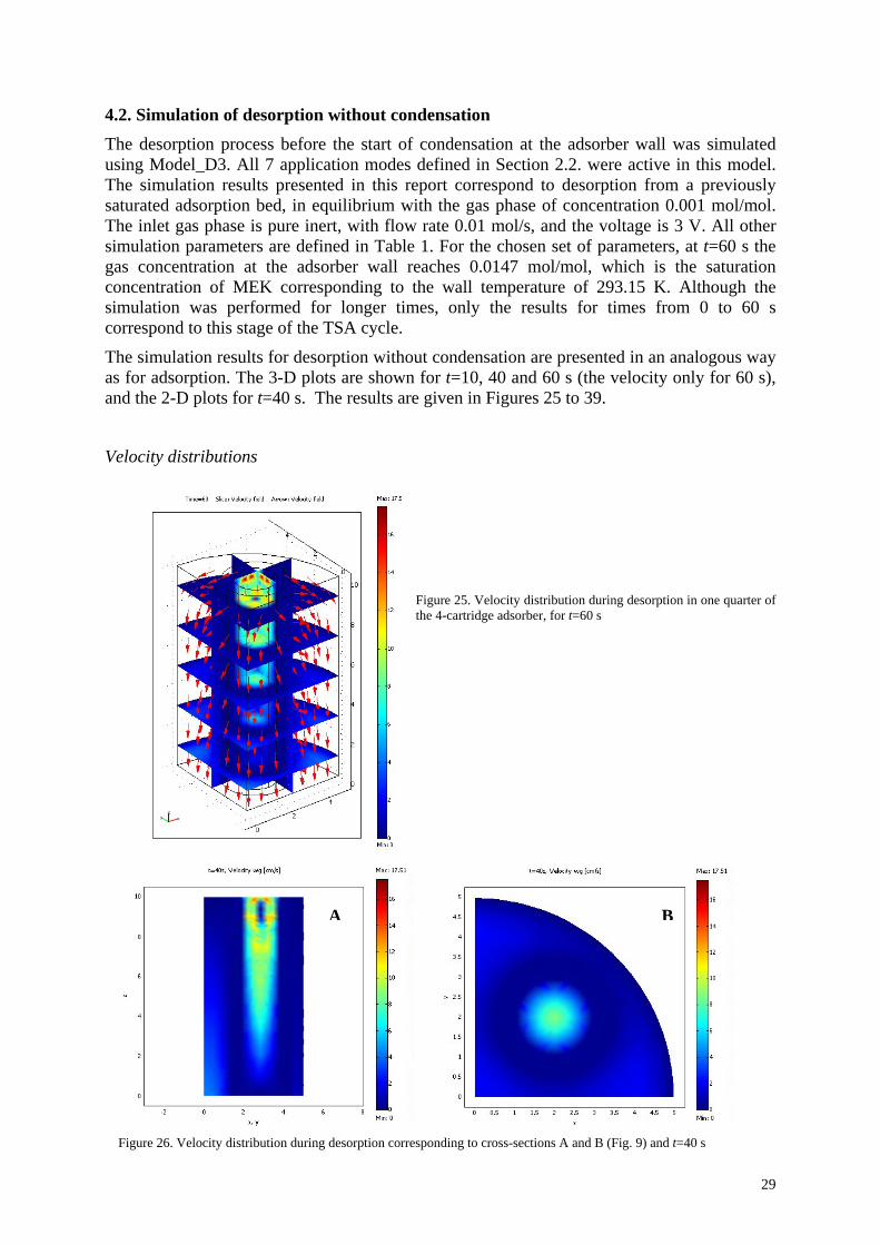
4.2. Simulation of desorption without condensation The desorption process before the start of condensation at the adsorber wall was simulated using Model_D3. All 7 application modes defined in Section 2.2. were active in this model. The simulation results presented in this report correspond to desorption from a previously saturated adsorption bed, in equilibrium with the gas phase of concentration 0.001 mol/mol. The inlet gas phase is pure inert, with flow rate 0.01 mol/s, and the voltage is 3 V. All other simulation parameters are defined in Table 1. For the chosen set of parameters, at t=60 s the gas concentration at the adsorber wall reaches 0.0147 mol/mol, which is the saturation concentration of MEK corresponding to the wall temperature of 293.15 K. Although the simulation was performed for longer times, only the results for times from 0 to 60 s correspond to this stage of the TSA cycle.
The simulation results for desorption without condensation are presented in an analogous way as for adsorption. The 3-D plots are shown for t=10, 40 and 60 s (the velocity only for 60 s), and the 2-D plots for t=40 s. The results are given in Figures 25 to 39.
Velocity distributions
Figure 25. Velocity distribution during desorption in one quarter of the 4-cartridge adsorber, for t=60 s
A B
Figure 26. Velocity distribution during desorption corresponding to cross-sections A and B (Fig. 9) and t=40 s
29
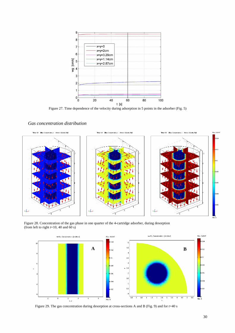
Figure 27. Time dependence of the velocity during adsorption in 5 points in the adsorber (Fig. 5)
Gas concentration distribution
Figure 28. Concentration of the gas phase in one quarter of the 4-cartridge adsorber, during desorption (from left to right t=10, 40 and 60 s)
B A
Figure 29. The gas concentration during desorption at cross-sections A and B (Fig. 9) and for t=40 s
30

Figure 30. Time dependence of the gas concentration during desorption in 5 points in the adsorber (Fig. 9)
Solid concentration distribution
Figure 31. Concentration of the solid phase in one quarter of the 4-cartridge adsorber, during desorption (from left to right t=10, 40 and 60 s)
B A
Figure 32. The solid concentration during desorption corresponding to cross-sections A and B (Fig. 9) and t=60 s
31

Figure 33. Time dependence of the solid concentration during desorption in 2 points in the adsorbtion bed (Fig. 9)
Gas temperature distribution
Figure 34. Temperature of the gas phase in one quarter of the 4-cartridge adsorber, during desorption (from left to right t=10, 40 and 60 s)
32
A B
Figure 35. The gas temperature during desorption, corresponding to cross-sections A and B (Fig. 9) and t=40 s
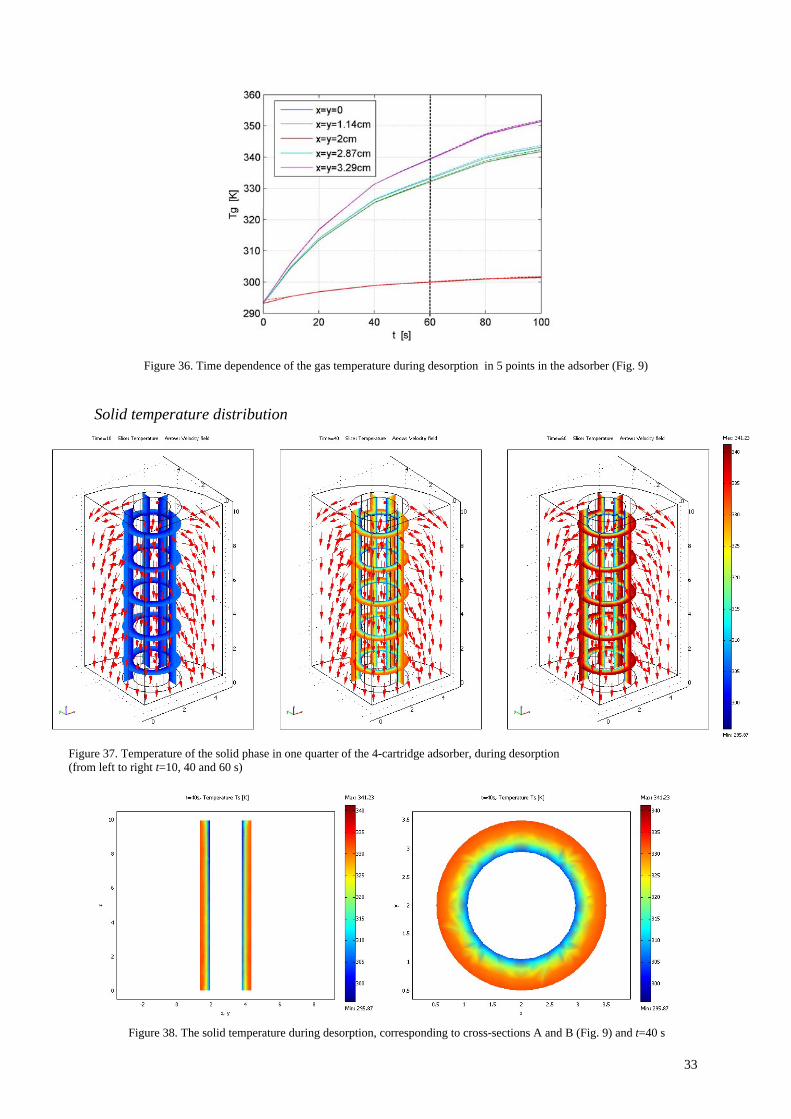
Figure 36. Time dependence of the gas temperature during desorption in 5 points in the adsorber (Fig. 9)
Solid temperature distribution
Figure 37. Temperature of the solid phase in one quarter of the 4-cartridge adsorber, during desorption (from left to right t=10, 40 and 60 s)
A B
Figure 38. The solid temperature during desorption, corresponding to cross-sections A and B (Fig. 9) and t=40 s
33
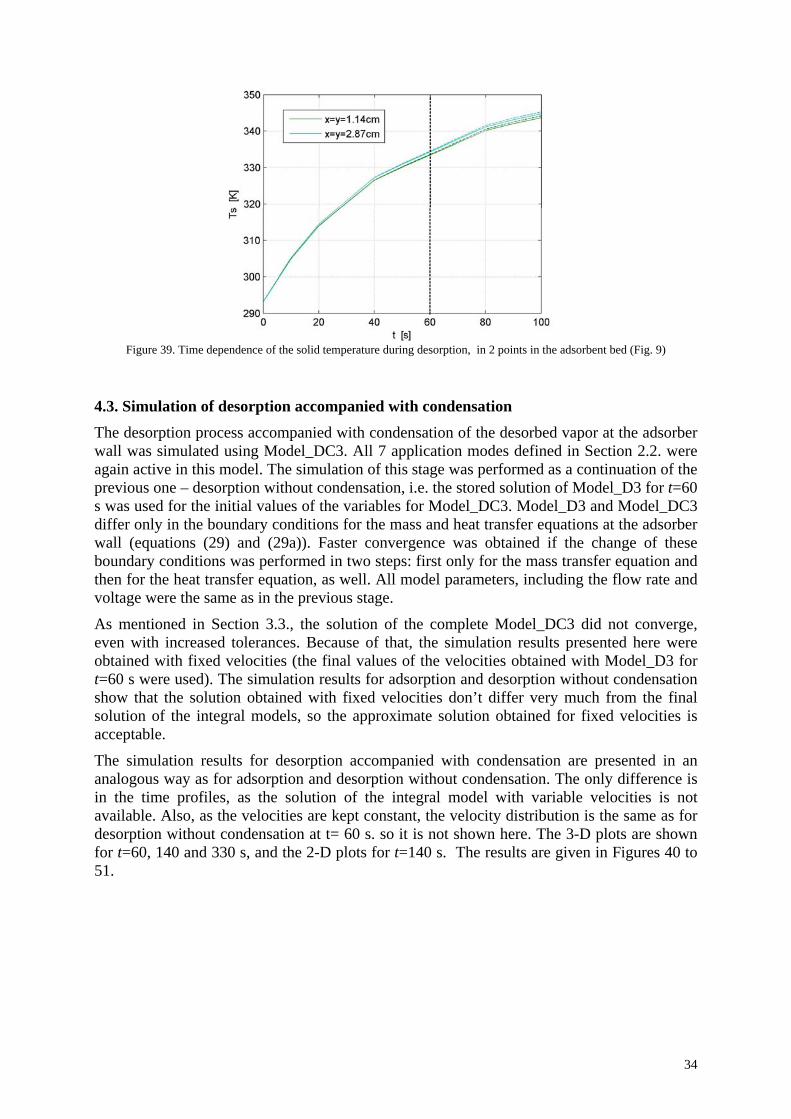
Figure 39. Time dependence of the solid temperature during desorption, in 2 points in the adsorbent bed (Fig. 9)
4.3. Simulation of desorption accompanied with condensation The desorption process accompanied with condensation of the desorbed vapor at the adsorber wall was simulated using Model_DC3. All 7 application modes defined in Section 2.2. were again active in this model. The simulation of this stage was performed as a continuation of the previous one – desorption without condensation, i.e. the stored solution of Model_D3 for t=60 s was used for the initial values of the variables for Model_DC3. Model_D3 and Model_DC3 differ only in the boundary conditions for the mass and heat transfer equations at the adsorber wall (equations (29) and (29a)). Faster convergence was obtained if the change of these boundary conditions was performed in two steps: first only for the mass transfer equation and then for the heat transfer equation, as well. All model parameters, including the flow rate and voltage were the same as in the previous stage.
As mentioned in Section 3.3., the solution of the complete Model_DC3 did not converge, even with increased tolerances. Because of that, the simulation results presented here were obtained with fixed velocities (the final values of the velocities obtained with Model_D3 for t=60 s were used). The simulation results for adsorption and desorption without condensation show that the solution obtained with fixed velocities don’t differ very much from the final solution of the integral models, so the approximate solution obtained for fixed velocities is acceptable.
The simulation results for desorption accompanied with condensation are presented in an analogous way as for adsorption and desorption without condensation. The only difference is in the time profiles, as the solution of the integral model with variable velocities is not available. Also, as the velocities are kept constant, the velocity distribution is the same as for desorption without condensation at t= 60 s. so it is not shown here. The 3-D plots are shown for t=60, 140 and 330 s, and the 2-D plots for t=140 s. The results are given in Figures 40 to 51.
34
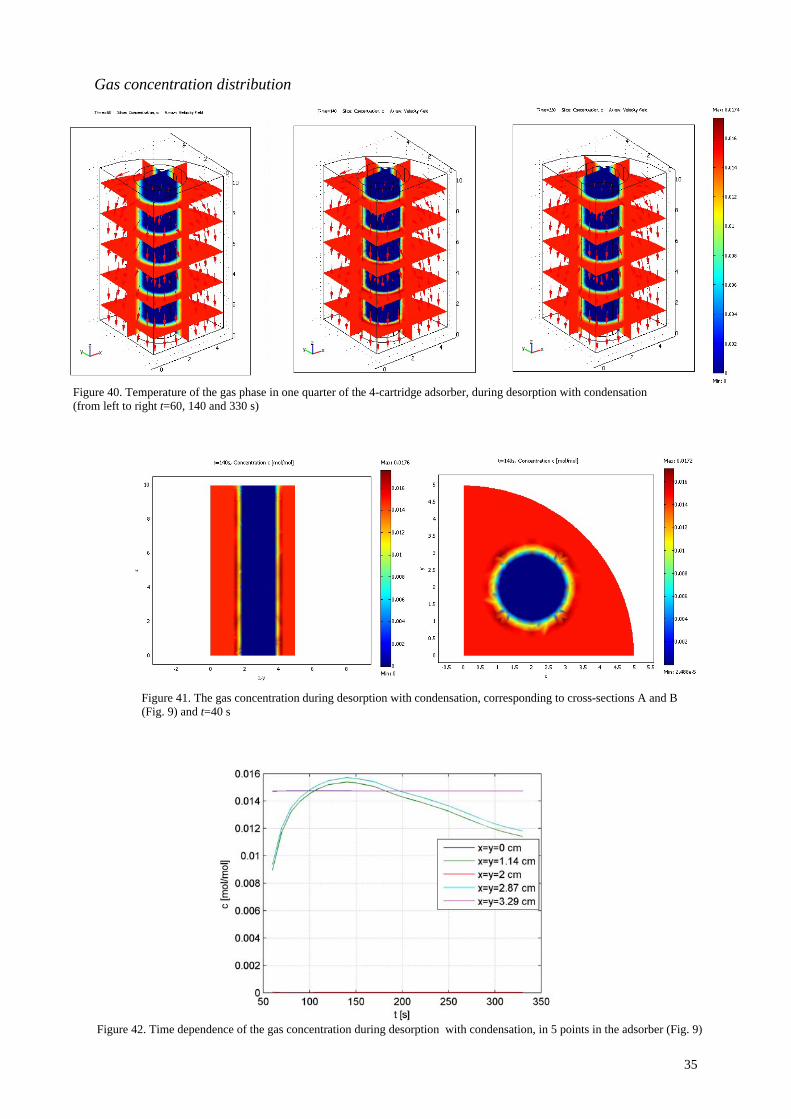
Gas concentration distribution
Figure 40. Temperature of the gas phase in one quarter of the 4-cartridge adsorber, during desorption with condensation (from left to right t=60, 140 and 330 s)
A B
Figure 41. The gas concentration during desorption with condensation, corresponding to cross-sections A and B (Fig. 9) and t=40 s
Figure 42. Time dependence of the gas concentration during desorption with condensation, in 5 points in the adsorber (Fig. 9)
35
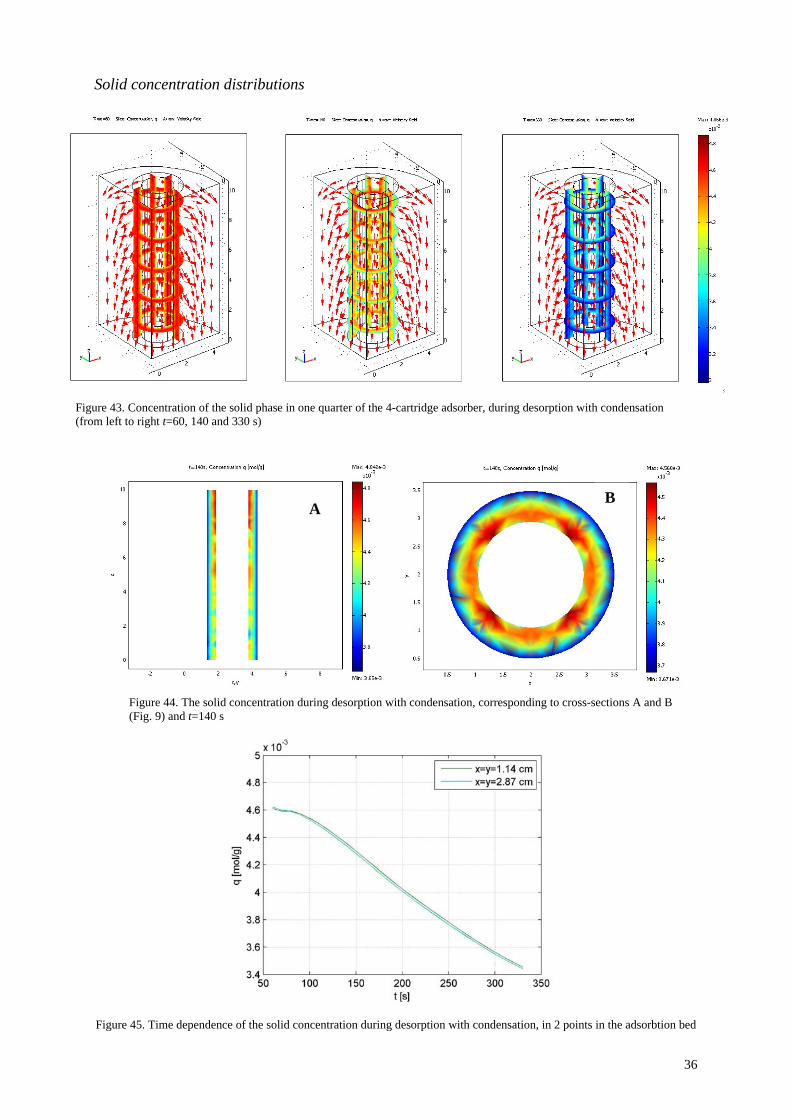
Solid concentration distributions
Figure 43. Concentration of the solid phase in one quarter of the 4-cartridge adsorber, during desorption with condensation (from left to right t=60, 140 and 330 s)
B A
Figure 44. The solid concentration during desorption with condensation, corresponding to cross-sections A and B (Fig. 9) and t=140 s
Figure 45. Time dependence of the solid concentration during desorption with condensation, in 2 points in the adsorbtion bed
36
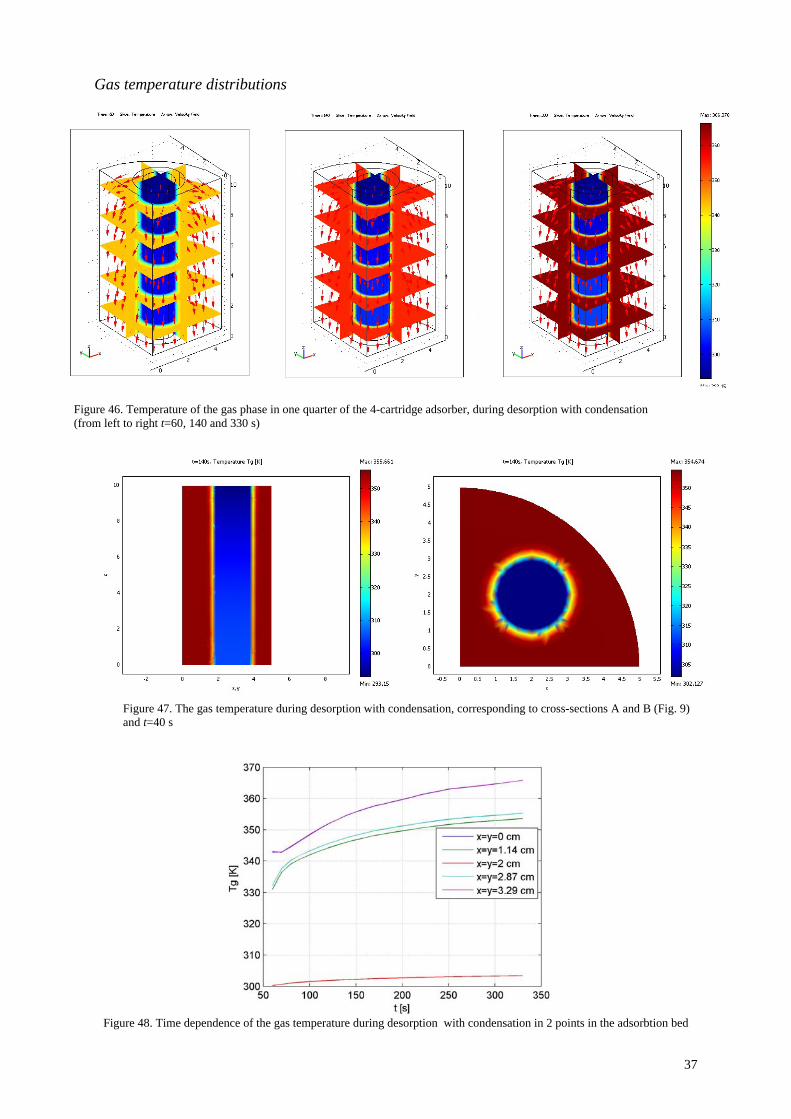
Gas temperature distributions
Figure 46. Temperature of the gas phase in one quarter of the 4-cartridge adsorber, during desorption with condensation (from left to right t=60, 140 and 330 s)
A B
Figure 47. The gas temperature during desorption with condensation, corresponding to cross-sections A and B (Fig. 9) and t=40 s
Figure 48. Time dependence of the gas temperature during desorption with condensation in 2 points in the adsorbtion bed
37
Solid temperature distributions
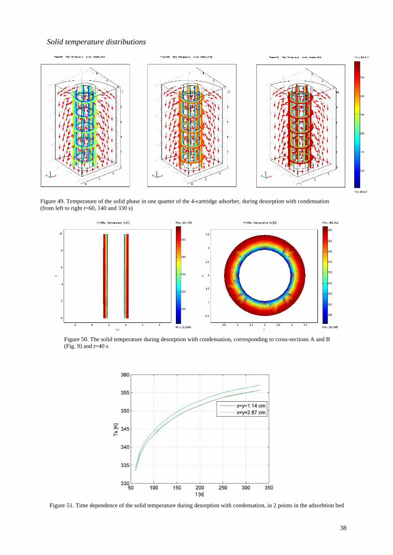
Figure 49. Temperature of the solid phase in one quarter of the 4-cartridge adsorber, during desorption with condensation (from left to right t=60, 140 and 330 s)
A B
Figure 50. The solid temperature during desorption with condensation, corresponding to cross-sections A and B (Fig. 9) and t=40 s
Figure 51. Time dependence of the solid temperature during desorption with condensation, in 2 points in the adsorbtion bed
38
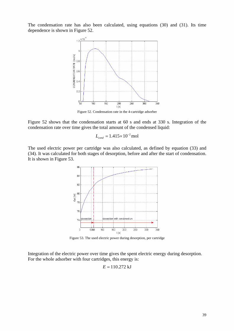
The condensation rate has also been calculated, using equations (30) and (31). Its time dependence is shown in Figure 52.
Figure 52. Condensation rate in the 4-cartridge adsorber
Figure 52 shows that the condensation starts at 60 s and ends at 330 s. Integration of the condensation rate over time gives the total amount of the condensed liquid:
mol10415.1 2−×=condL The used electric power per cartridge was also calculated, as defined by equation (33) and (34). It was calculated for both stages of desorption, before and after the start of condensation. It is shown in Figure 53.
Figure 53. The used electric power during desorption, per cartridge
Integration of the electric power over time gives the spent electric energy during desorption. For the whole adsorber with four cartridges, this energy is:
kJ272.110=E
39
5. Conclusions
The objective of this phase of the project: to model the TSA system with an adsorber with four parallel, cartridge-type adsorbers, raised a very difficult and demanding task, even when using an excellent modeling tool, such as COMSOL Multiphysics. It was necessary to build 3-D models of a very complex system, with complex geometry and a large number of interacting phenomena and processes. Even when the problem was reduced to modeling of only one quarter of the adsorber (assuming that all four cartridges in the adsorber were identical), seven interacting application modes needed to be incorporated into a 3-D model geometry consisting of 3 sub-domains. This resulted with a very large number of degrees of freedom, i.e., with a large number of coupled nonlinear differential equations that needed to be solved numerically.
The first problem associated with that was a very high demand regarding computer memory. A rather coarse mesh had to be used in order to enable solving of the models on a personal computer with 4 GB RAM.
The second problem was diverging of the solution. The complete models did not converge. For that reason, a step-by-step solution procedure had to be developed. For the model of desorption with condensation, even this procedure failed, and only an approximate solution of the model with fixed velocities could be obtained. We believe that this procedure could help other researchers in solving their difficult 3-D problems.
The third problem was in relatively long computing times. For example, when solving the model for adsorption, we needed ~200 s for Step 1, ~1150 s for Step 2 and ~4300 s for Step 3.
Nevertheless, in spite of all these problems, we succeeded in postulating and solving the models describing all three stages of the TSA process in the 4-cartridge adsorber.
We believe that the convergence problems are partly associated with the coarse mesh used, and that using a finer mesh would improve the convergence, on account of a larger computer memory and longer computer times. Of course, this would demand using of a much faster computer with more memory.
With this phase of the project we completed mathematical modeling of the adsorber configurations developed in the group of Prof. Rood. These models can be used for simulation, optimization of the process parameters and adsorber geometry, but also for comparison between different configurations. Nevertheless, for practical applications of these models, it would be necessary to have accurate physical and transport parameters for the particular system. Usually, such parameters have to be estimated from experimental data. Also, more accurate solution of the mathematical models, obtained with finer mesh and lower tolerances, would be needed, which is directly related to the computer hardware. This is especially important for the 3-D models developed in this phase of the project.
The set of mathematical models developed in the three phases of the project offer a good basis for optimization of the TSA processes with electrothermal desorption.
40
Nomenclature
a (m2/m3) - Specific surface area
b (K-1) - Temperature coefficient of the bed electrical resistivity
C (mol/mol) - Adsorbate concentration in the gas phase
C*(mol/mol) - Adsorbate concentration in the gas phase in equilibrium with the solid phase
Csat (mol/mol) - Saturation concentration
cpg (J/mol/K) - Specific heat capacity of the inert gas
cpl (J/mol/K) - Specific heat capacity of liquid adsorbate
cps (J/g/K) - Heat capacity of the solid phase
cpv (J/mol/K) - Specific heat capacity of gaseous adsorbate
Dm (mol/cm/s) - Mass transfer dispersion coefficient
Dthg (W/K/cm) - Heat diffusivity of the gas phase
Dths (W/K/cm) - Heat diffusivity of the solid phase
E (J/mol) - Adsorption energy of the adsorbate (D-R eq.)
g (cm/s2) - Gravitation constant
G (mol/s) - Flow rate of the inert gas
H (cm) - Bed axial dimension (Fig. 7)
hb (J/cm2/K) - Solid to gas heat transfer coefficient
hs1 (J/cm2/K) - Heat transfer coefficient from the solid phase to the gas phase in the central tube(s)
hs2 (J/cm2/K) - Heat transfer coefficient from the solid phase to the gas phase in the annular tube
hwg (J/cm2/K) - Gas to ambient heat transfer coefficient (heat losses)
J (A/cm2) - Current density
Jcond (mol/cm2/s) - Condensation flux
k (cm2) - Asorbent bed permeability
km (mol/cm2/s) - Mass transfer coefficient in the adsorbent bed
km1 (mol/cm2/s) - Mass transfer coefficient between the adsorbent bed and the gas in the central tube
km2 (mol/cm2/s) - Mass transfer coefficient between the adsorbent bed and the gas in the annular tube
condL& (mol/s) - Flow-rate of the condensed liquid
Lcond (mol) - Total amount of the condensed liquid
p (Pa) - Gas pressure
pA (Pa) - Adsorbate partial pressure
pc (Pa) - Critical pressure
p0 (Pa) - Adsorbate saturation pressure
elQ& (W) - Rate of heat generation (equal to electric power)
Qel (J) - Heat generation (equal to electric energy)
q (mol/g) - Adsorbate concentration in the solid phase
Rg (J/mol/K) - Gas constant
41

r1 (cm) - radius of the central tube (Fig. 7)
r2 (cm) - outer radius of the adsorbent bed (Fig. 7)
r1 (cm) - radius of the adsorber vessel (Fig. 7)
Ta (K) - Ambient temperature
Tg (K) - Gas phase temperature
Tc (K) - Critical temperature
TR (K) - Referent temperature
Ts (K) - Solid phase temperature
Tw (K) - Wall temperature
t (s) - Time
U (V) - Electric potential
U0 (V) - Supply voltage
u (cm/s) - x-component of the gas velocity
VPA, VPB, VPC, VPD - Wagner constants
v (cm/s) - y-component of the gas velocity
W (cm3/g) - Adsorbate volume per 1 g of the adsorbent mass
W0 (cm3/g) - Total volume of micropores (D-R equation)
w (cm/s) - z-component of the gas velocity
x (cm) - x - coordinate
x0 (cm) - position of the cartridge center in the x-direction
y (cm) - y - coordinate
y0 (cm) - position of the cartridge center in the y-direction
z (cm) - z - coordinate
Greek letters:
∆Hads (J/mol) - Heat of adsorption
∆Hcond (J/mol) - Heat of condensation
εb - Bed porosity
µ (Pa/s) - Dynamic viscosity
ρ (Ωcm) - Electric resistivity
ρ0 (Ωcm) - Electric resistivity at referent temperature TR
ρg (mol/cm3) - Gas phase density
ρb (g/cm3) - Adsorbent bed density
ρA (g/cm3) - Adsorbate density
42
Subscripts:
b - bed
g - gas
in - inlet
i,o - inner and outer tube
out - outlet
p - previous (initial)
s - solid phase
it - inner (central) tube
ot - outer (annular) tube
x - x-direction
y - y-direction
z - z-direction
43
References: 1. Fabuss, B.M. and W.H. Dubois, “Carbon Adsorption-Electrodesorption Process”,
63rd Annual Meeting of the Air Pollution Control Association, St. Louis, Missouri (1970)
2. Petkovska, M. et al, “Temperature-swing gas separation with electrothermal desorption step”, Sep. Sci. Technol., 26, 425-444 (1991)
3. Petkovska, M.; Mitrović, M., “Microscopic modelling of electrothermal desorption”, Chem. Eng. J. Biochem. Eng. J, 53, 157-165 (1994a)
4. Petkovska M. and Mitrović M., “One-dimensional, non-adiabatic, microscopic model of electrothermal desorption process dynamics”, Chem. Eng. Res .Des., 72, 713-722 (1994b)
5. Sullivan P., “Organic vapor recovery using activated carbon fiber cloth and electrothermal desorption”, Ph.D. Thesis, University of Illinois at Urbana-Champaign (2003)
6. Bathen, D., “Gasphasen - Adsorption in der Umwelttechnik - Stand der Technik und Perspektiven”, Chemie Ingenieur Technik, 74, 209-216 (2002)
7. Subrenat A. and Le Cloirec P, “Industrial application of adsorption onto activated carbon cloths and electro-thermal regeneration”, J. Environ. Eng., 130, 249-257 (2004)
8. Sullivan P. et al, “Capture of Organic Vapors Using Adsorption and Electrothermal Regeneration”, J. Environ. Eng., 130, 258-267 (2004)
9. Rood M. et al, “Selective sorption and desorption of gases with electrically heated activated carbon fiber cloth element” US Patent No. 6,346,936 B1(2002)
10. Petkovska M., “Rigorous Mathematical Modeling of Adsorption System with Electrothermal Regeneration of the Used Adsorbent”, Final Performance Report for Project No. FA8655-03-1-3010, Year 1 (2004)
11. Petkovska M., Antov-Bozalo D., Markovic A., “Rigorous Mathematical Modeling of Adsorption System with Electrothermal Regeneration of the Used Adsorbent”, Final Performance Report for Project No. FA8655-04-1-3010, Year 2 (2005)
12. Dombrowski K.D. et al, “Organic Vapor Recovery and Energy Efficiency during Electric Regeneration of an Activated Carbon Fiber Cloth Adsorber”, J. Environ. Eng., 130, 268-275 (2004)
44
Recommended