NASA
Contractor Report 4641
Army Research Laboratory
Technical Report ARL-TR-645
SEEK_A Fortran Optimization ProgramUsing a Feasible DirectionsGradient Search
M. SavageThe University of AkronAkron, Ohio
Prepared for
Propulsion Directorate
U.S. Army Aviation Systems Commandand
Lewis Research Center
under Grant NAG3-1047
National Aeronautics and
Space Administration
Office of Management
Scientific and Technical
Information Program
1995
https://ntrs.nasa.gov/search.jsp?R=19950014942 2018-05-26T18:13:13+00:00Z


SEEK - a Fortran Optimization Program
Using a Feasible Directions Gradient Search
M. Savage
The University of Akron
Akron, Ohio 44325
Grant NAG3-1047
Abstract
This report describes the use of computer program 'SEEK' which works in
conjunction with two user-written subroutines and an input data file to
perform an optimization procedure on a user's problem. The optimization
method uses a modified feasible directions gradient technique. SEEK is
written in ANSI standard Fortran 77, has an object size of about 46 K bytes
and can be used on a personal computer running DOS. This report describes the
use of the program and discusses the optimizing method. The program use is
illustrated with four example problems: a bushing design, a helical coil
spring design, a gear mesh design and a two-parameter Weibull life-reliability
curve fit.

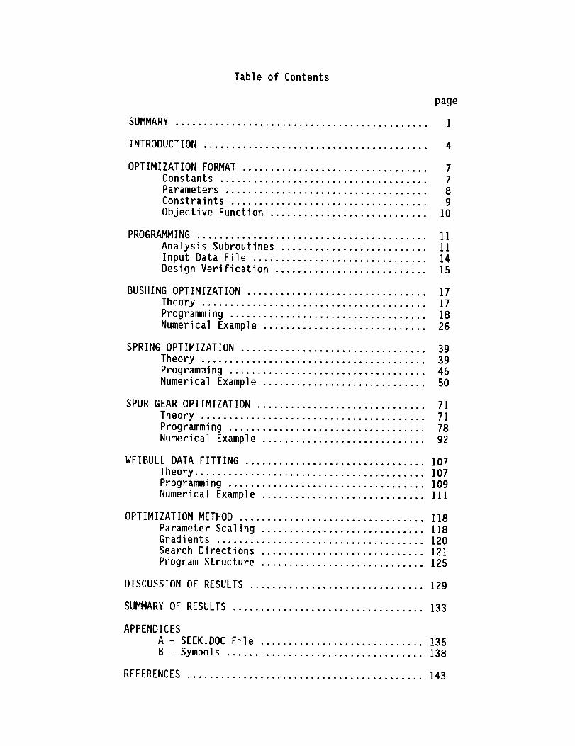
Table of Contents
page
SUMMARY ............................................. I
INTRODUCTION ........................................ 4
OPTIMIZATION FORMAT ................................. 7
Constants ..................................... 7
Parameters .................................... 8
Constraints ................................... 9
Objective Function ............................ ]O
PROGRAMMING ......................................... 11
Analysis Subroutines .......................... II
Input Data File ............................... 14
Design Verification ........................... 15
BUSHING OPTIMIZATION ................................ 17
Theory ........................................ 17
Programming ................................... 18
Numerical Example ............................. 26
SPRING OPTIMIZATION ................................. 39
Theory ........................................ 39
Programming ................................... 46
Numerical Example ............................. 50
SPUR GEAR OPTIMIZATION .............................. 7I
Theory ........................................ 71
Programming ................................... 78
Numerical Example ............................. 92
WEIBULL DATA FITTING ................................ 107
Theory ......................................... 107
Programming ................................... 109
Numerical Example ............................. 111
OPTIMIZATION METHOD ................................. 118
Parameter Scaling ............................. ]18Gradients ..................................... 120
Search Directions ............................. 121
Program Structure ............................. 125
DISCUSSION OF RESULTS ............................... 129
SUMMARY OF RESULTS .................................. 133
APPENDICES
A - SEEK.DOC File ............................. 135
B - Symbols ................................... 138
REFERENCES .......................................... 143


SUMMARY
This report describes the use of a computer program, 'SEEK' for
engineering design optimization. The program is not complete in itself in
that it is written to work with problem specific user subroutines and an input
data file. It performs a gradient search optimization of the user's problem
to find an optimal set of design parameter values. Optimization is performed
using a modified feasible directions gradient technique. The program is
written in ANSI standard Fortran 77 and has an object size of about 46 K bytes
for the optimizing code alone for use on a personal computer running DOS. Its
source code is about 1,200 lines in length and its size is 39 K bytes.
In the OPTIMIZATIONFORMATsection, the four interface vectors to the
procedure are described. These vectors are: I) the problem constants, 2) the
independent design parameters, 3) the constraint bounds, and 4) the objective
function terms. The problem constants and independent design parameter values
define a specific trial design. In the optimization, the program varies the
design parameter values to search for the design which has the best objective
function value while satisfying the constraint bounds.
In the PROGRAMMINGsection, the report describes the two analysis
routines, BOUNDSand VALUESwhich the user must write to evaluate the
constrained functions and the objective function. BOUNDStakes as input the
constant and design parameter vectors and produces a vector of the constrained
function values as its output. VALUEStakes as input the sameconstant and
design parameter vectors and produces the objective function value vector as
its output. The format and make-upof the input data file which gives the
four vectors of constants, design parameters, constraint limits and objective
function weighting coefficients are described. In this file, extensive
labeling for the four vectors is included. The design verification feature of
the optimization program is described also. Once a numerical optimum is
found, the program provides the user the opportunity to try alternate designs
for comparison purposes.
To illustrate the use of the program, four examples are presented:
I) a bushing design, 2) a helical coil spring design, 3) a spur gear mesh
design, and 4) a Weibull data curve fit. The bushing design problem is to
find the length and diameter of a bushing to minimize the friction torque in
the bearing for a given load and material properties. The spring design is to
find the wire diameter and meancoil diameter which support a given
alternating load with a required stiffness. Three different design objectives
of minimumspring weight, minimumspring height and minimumcoil volume are
sought. The gear design is to determine the numberof pinion teeth, diametral
pitch and face width for a compact spur gear set to transmit a given power at
a given input speed with a given speed reduction. Twoobjectives are sought:
I) minimumcenter distance for a desired life and 2) maximumlife for a given
center distance. The fourth example showsthe fitting of a two-parameter
Weibull distribution to life data for a series of identical units tested at
the sameload.
Each example includes an analysis of the problem, the organization of
the optimization variables, the writing of the analysis subroutines and the
input data file for a specific problem, the compiling and running of the
program, the use of design verification to obtain reasonable values and an
interpretation of the output data file. In each case, the design verification
opportunity leads to the discovery of a practical solution with near optimal
characteristics.

After the examples, the OPTIMIZATIONMETHODsection presents a
description of the gradient search method with its three modesof operation:
I) unconstrained searching, 2) acceptable design searching, and 3) feasible
direction searching along one or more design constraints. The unconstrained
searching modeemploys the gradient in the objective function to improve the
design at the fastest rate when possible. The acceptable design searching
uses the sumof the gradients in the violated constraints to find the
acceptable design region. And, the feasible direction searching modecombines
the gradients in the objective function and the violated constraints to
improve the objective function value while keeping the trials within the
acceptable design region. This section concludes with a description of the
program structure and operation.
INTRODUCTION
Optimization is a mathematical process of seeking the most favorable
combination of parameters to achieve the best outcome possible [I-3]. In
design, one constantly searches for an ideal trade-off of conflicting
performance objectives. For aircraft transmissions, for example, we might
wish to obtain the lightest transmission which has someminimumacceptable
service life, or we maywant to maximize the service life at a given
transmission weight [4]. These objectives are sought throughout the design
and development process with repetitive design descriptions and evaluations -
on paper or CADlayout at the design stage and in hardware at the prototype
stage. Manyof the optimizing, trade-off decisions which develop and improve
the product are madeby engineers without the help of mathematical models of
the product's performance.
Optimization offers the promise of assistance with the difficult trade-
off decisions at the early stages of the design, before costly prototypes are
constructed and tested [5]. A spectrum of optimization codes have been
written to assist in the design of complex structures which can be modeled
with large matrices of simultaneous linear equations [2,3]. With an objective
computer search through the space of potential designs, we are given a greater
chance of determining a truly optimum design.
Unfortunately, manymechanical design problems cannot be described by a
set of linear equations. The size of the problem as measuredby the numberof
independent design parameters and the constraints which are to be satisfied
may be small. But the complexity of the problem may be large due to the non-
linear and often discontinuous nature of the design property and constraint
relations. This combination keeps the optimization of mechanical designs in
4

the realm of an art which requires considerable engineering insight to
complement the available mathematical models and computer solutions {6].
In modeling mechanical systems, one is often confronted with the choice
of obtaining exact solutions to an approximate model or obtaining approximate
solutions to an exact model. With the designer active in the process, rapid
solutions of an approximate model can lead to practical optimal designs even
whenthe mathematical optimum contains someflaws {7]. Modified gradient
optimization techniques such as the feasible directions method are quite
powerful and rapid when they have continuous models in which gradients can be
calculated. The method of this optimization is to have the engineer write
Fortran subroutines which model the design with continuous properties as
functions of the constants and independent design parameters which define the
design. The optimizer can then find the optimal solution to this 'ideal'
problem and report it to the engineer to allow a check of alternate designs
which satisfy additional constraints of practicality. The end result is a
practical, optimal design.
This report describes the use and background of a Fortran program, SEEK,
which is written to assist the mechanical designer in developing balanced
optimal designs. The intent of the program is to keep the engineer in the
process while providing a systematic search of potential designs. In doing
this, it allows the engineer to use the mathematical models of the
optimization to evaluate near optimal, practical designs. SEEK,which
requires two user-written analysis subroutines, reads its input from an ASCII
data file and writes the output of the optimization both to the screen and to
an output ASCII log file. To document the optimization clearly, the input

data file includes a significant amountof text to describe the numerical
values in the output file.
The report includes an OPTIMIZATIONFORMATsection which describes the
basic format of the optimization problem: the constants, design parameters,
constraint bounds and objective function; as well as a PROGRAMMINGsection,
which describes the programmingrequired to prepare SEEKfor use in an
interactive design session. This section describes: the two analysis
subroutines, the input data file, the use of the program with changes to the
input file and design verification in the interactive session.
To demonstrate the power and ease of use of this optimization procedure,
several small design examples follow in the next sections: a bushing, a
spring, a spur gear mesh, and the fitting of a two parameter Weibull
distribution to experimental test data.
An OPTIMIZATIONMETHODsection follows which describes the structure and
operation of the optimization code. This code is small with 1200 lines and
less than 40 k bytes so the optimization can be performed on a personal
computer running with DOS. The speed of a 486 machinemay becomeattractive
for the more complex analysis models.

OPTIMIZATIONFORMAT
An optimization problem may be formulated as a constrained search in
terms of four vectors and two sets of relations. In this formulation, only
inequality relations are used for the constraints. The four vectors are:
I) the constants of the problem which do not change for a given design, 2) the
parameters which define a design and which are the sought values, 3) the
constraint values which may be upper or lower bounds on properties of the
design, and 4) the objective function's weighting coefficients.
In this formulation, at least two Fortran subroutines are needed:
I) BOUNDSwhich evaluates the constrained variable values _n terms of the
constants and design parameter values and 2) VALUES which evaluates the
objective function's value for a given set of constants and design parameter
values. These two subroutines combine with the input data file to define the
specific problem for optimization. The gradient calculations which perform
the optimization by calling these two subroutines repeatedly and the input and
output file interfacing are contained in the SEEK Fortran code.
Constants
Each problem is defined by a series of constant values such as: size,
power level, speed of operation, elastic modulus, material strength or
requested service life. These constants are fixed for all trial designs of
the optimization effort, and the constrained properties and objective function
values are direct functions of them. The constants may change for a different
design using the same analysis subroutines, however. For example, designs
made of steel will have different properties from those made of nylon, yet
each steel design will have the same material stiffness and strength as the
other steel designs.

The program will read these constants and their labels from the ASCII
input file, store them in arrays and use the values whenever the constrained
property or objective function values are calculated.
Parameters
In each problem, we are searching for a set of parameter values which
optimize the objective function to either a minimum or a maximum value. These
parameters are the second vector entered in the input data file. The
optimization scheme proceeds by analyzing repeated trials until it selects one
for which the analysis yields an optimum objective function value. So the
values entered for the design parameters include an initial value for each
parameter for the first trial analysis. This vector also includes upper and
lower values for each design parameter. These upper and lower values serve to
establish the relative sensitivity of the parameter for the gradient searches,
but do not limit the value itself. By increasing the span between the upper
and lower values for a design parameter, the user can increase the sensitivity
of that parameter in the design search. If it appears that a design parameter
is not changing as the optimizer seeks out better designs, increasing this
span between the upper and lower values will increase its tendency to change
in future optimization runs.
After reading these parameter values and their labels from the input
file, the program will store them in arrays, use the parameter ranges to set
relative sensitivities which will not change throughout the optimization and
place the initial parameter values into the parameter array. The parameter
array will change throughout the operation of the program until it contains
the values of the parameters which optimize the objective function.
Constraints
Limiting each design is a series of constraints on the properties of the
design. These constraints may be applied directly to one or more of the
parameters such as the thickness of a beam or they may be applied to a
calculated property of the design such as the maximum stress in the beam. The
constraints of this algorithm are inequality constraints. In the general
optimization formulation, two types of constraints are possible: inequality
and equality. Gradient search algorithms require a continuum of parameter and
property values in which to move around in search of the optimum. Inequality
constraints provide boundaries to the design space but do not diminish it.
Equality constraints reduce the space by one dimension. Each equality
constraint transforms one independent design parameter into a dependent design
parameter. There are two ways to include an equality constraint in this
algorithm: I) reduce the design space by one, or 2) enter the equality
constraint into the data as an inequality constraint.
The first method is the best because it simplifies the calculations
making the optimization more direct and faster. If the width of a rectangular
spring is always seven times its height, then one can remove the width from
the list of independent design parameters and set it equal to seven times the
height in the calculations. This reduces all gradient calculations by one
element and leaves a full design space for the remaining parameters' gradient
searches.
The second method may be easier to implement if the equality constraint
is not tied to the parameters directly. By entering it as an inequality
constraint, one leaves the design space at its larger dimensional size and
cuts it in half with the bounding value. Since the unbounded optimal design

would probably lie off this constraint, placing this bound between the
unboundedoptimum and the acceptable design space will place the bounded
optimal design right on this constraint and thus actually satisfy the equality
constraint.
The program will read these constraints, their directions and their
labels from the input file, place them in arrays and use them in the
subroutine BOUNDS,which is provided by the user, to limit the acceptable
design space throughout the optimization.
Objective Function
In each optimization, some property or combination of properties, called
the objective function, is to be minimized or maximized. The weighting
coefficients of these properties are the last vector entered in the input data
file. These coefficients may be percentages, unit conversions to place the
properties in the same dimensions or they may be switches such as zero and one
to change the optimization in the data file by changing the sought objective.
The assumption is that the objective function to be optimized may be expressed
as a linear sum of terms, each with its own weighting coefficient. The
weighting coefficients and direction of optimization will remain fixed
throughout the optimization.
The program will read these coefficients and their labels from the end
of the input data file, place them in arrays and use the coefficients to
modify the objective function property values. These values are calculated in
subroutine VALUES which is provided by the user.
10

PROGRAMMING
With these four vectors defined and labeled, the program starts the
output file with an echo of the input data to document the optimization
problem. It then proceeds to seek an optimal design with the modified
feasible directions gradient method. Using gradients in the objective
function and in the violated constraints, the program can move from an initial
design which does not satisfy the design constraints to designs which are
valid. It can also improve a valid initial design to obtain an optimum design
within the assumptions of the model.
Once an optimum design is found, the program prints: the found design
parameters, the objective function value with its componentfunction values,
and the constraints with both their design and limit values. The program then
offers the user the opportunity to try alternate designs. On receiving the
revised design parameter values, the program uses subroutines BOUNDSand
VALUESto check this design, prints out its properties and offers the user the
chance to try another alternate design. All design trials are printed to the
screen and the ASCII output log file.
Analysis Subroutines
To model a problem, the program needs two analysis subroutines: BOUNDS
and VALUES. These subroutines are problem specific and should match the input
data. Subroutine BOUNDS calculates the constrained property values for each
design trial and gradient perturbation as direct functions of the constants
and design parameters only. Data are passed to BOUNDS with two dynamically
dimensioned arrays: CONST(NCO) for the constants and X(NX) for the design
parameters, and the constraint value results are returned to the program in
the array VCSTR(NCS). Subroutine VALUES calculates the objective function
11

values also as direct functions of the constants and design parameters only.
Data are passed to VALUES with the same two arrays: CONST(NCO) for the
constants and X(NX) for the design parameters, and the object function values
are returned in the array OBJECT(NOB).
Both subroutines must be able to determine their outputs as continuous
functions over the range of design parameters used. Since small perturbations
are given to the design parameters to determine corresponding changes in the
objective function value and in the constrained variable values throughout the
design search, the subroutine calculations must be defined and continuous.
Discrete parameter requirements such as integer tooth numbers for gears and
standard component sizes can be added by the user in the verification stage of
the optimization process. They cannot be included in the simulation model
itself.
These subroutines may contain formulas, interpolated data, iterations or
other subroutines as long as the resulting calculations yield continuous
functions of the design parameters. If the subroutines call other
subroutines, they should not have the same names as those subroutines included
in the optimizing part of SEEK, which are listed in Table I.
Common blocks may be used by the subroutines, but SEEK uses four common
blocks, which should not be altered: CURVE, PAR, VAR, and UNITS. One of these
common blocks, UNITS, contains four integer variables, NW, NR, NF and ND.
These are the file numbers for writing and reading to the interface devices.
NW identifies the screen, NR identifies the keyboard, NF identifies the output
file and ND identifies the input file. The user may add additional
information to the output with these file numbers, bearing in mind that BOUNDS
and VALUES are called many times by SEEK in the optimization process.
12

Table I
Subroutines of Proqram SEEK
Line
756
983
1207
1113
1033
1174
724
912
874
740
1088
1210+
1146
Name
BACK
BOUNCE
BOUNDS
CHECK
GRADNT
MERIT
RESIZE
SCAN
SCOUT'
SIZE
UNIT
VALUES
WALL
Function
Search for Acceptable Design Space
Find Gradient Sum of the Violated Constraints
User Supplied Constraint Analysis
Test for Constraint Violation
Evaluate a Gradient
Evaluate the Objective Function Sum
Unscale the Design Parameters into Real Units
Increment the Design in the Acceptable Design
Space
Try a New Design Position And Check the
Constraints
Scale the Design Parameters to Unit Space
Normalize a Vector
User Supplied Objective Function Analysis
Evaluate a Specified Constraint
13

Input Data File
Coordinated with these two required subroutines is the ASCII input data
file, which is described in Appendix A - SEEK.DOC. The initial line in the
data file is a text line of fifty characters or less which describes the
design being optimized. This is followed by a line which contains a single
number, NCO, - the number of constant values to follow, which is the first
vector in the data file. Each optimization constant is then entered in a set
of three lines: I) the numerical value, 2) the name of the constant in thirty
characters or less, and 3) the units for the constant in twelve characters or
less. With this information, the program will label the constant values
whenever it prints them.
Following the constants in the input data file is the list of
independent design parameters, which is the second vector. After the last
constant has been listed, the next line is once again a single number, NX, -
the number of parameter values to follow. Each parameter is then entered in a
set of three lines: I) three numerical values - a low estimate for the
parameter, a high estimate and an initial estimate; 2) the name of the
parameter in thirty characters or less; and 3) the units for the parameter in
twelve characters or less.
The list of constraint bounds is the third vector. After the last
parameter has been listed, the next line is a single number, NCS, - the number
of constraint bounds to follow. Each bound is then entered in a set of three
lines: ]) the word 'UPPER' or 'LOWER' followed by the numerical value
including its decimal point, 2) the name of the constraint in thirty
characters or less, and 3) the units of the constraint in twelve characters or
less.
14

Finally, the list of weighting coefficients is the fourth vector
entered. After the last constraint has been listed, the next line is a three
letter prefix, 'MIN' or 'MAX', which describes the direction of optimization.
This is followed by a line with a single number, NOB, - the number of
weighting coefficients to follow. Each coefficient is then entered in a set
of three lines: I) the numerical value, 2) the nameof the property in thirty
characters or less, and 3) the units for the property in twelve characters or
less.
Desiqn Verification
As described at the start of this section, the use of SEEK is somewhat
interactive. Because the user must add at least two subroutines to the
program in addition to the input data file, the combined program must be
compiled separately for each optimization application. After writing the
analysis subroutines with the proper dynamic dimensioning in the calling
arguments, the user may add subroutines to the end of the source code for SEEK
and compile the program in the environment in which it is to be run. The
compiler should be a Fortran 77 compiler of which there are several PC
versions available. Once compiled and linked into an executable program, the
optimizer can be run with the matching data file to find an optimal design.
With the interaction of the data file and the analysis subroutines, the
user may change the way an optimization is conducted through small changes in
the data file. By using one and zero as weighting coefficients to an
objective function that contains totally different terms and by switching
constraints from UPPER to LOWER or changing their values to make them active
or inactive, one can change an optimization significantly.
15
For example, one could have a transmission life optimization program
which included bounds on the transmission size and life as well as terms in
the objective function for size and life E81. By requesting that the size be
less than somevalue, that the life be greater than zero and by having a
weighting coefficient of one for life and zero for size and by selecting 'MAX'
in the input data file, one would have an optimization that would maximize the
life of the transmission within a given acceptable size. Shifting the
requests in the input file to request that the size be greater than zero, that
the life be greater than somedesired value, and by having a weighting
coefficient of zero for life and one for size with 'MIN' selected in the input
data file would minimize the size of the transmission for the requested
service life.
Smaller changes in limit values or problem constants could change the
size of a requested design or someother feature without requiring a change in
the compiled program. As stated earlier, the program generates a complete log
file of the obtained designs and the verified designs in response to keyboard
input after an 'ideal' design has been found and written to the screen and the
log file. Speed of execution of the program is entirely dependent upon the
complexity of the analysis models. Small optimization programs can run
quickly on the personal computer. The following four sections will
demonstrate the use of SEEKfor several different design optimizations.
16

BUSHINGOPTIMIZATION
Four examples of increasing complexity will be presented to illustrate
the capability of SEEK. The first example is that of the design of a low-
speed bearing to support a radial shaft load. For this application, the
simplest bearing is a bushing which is defined by its material, length and
diameter.
Theor_
Consider the design of a bushing to support a radial shaft load. With
little or no lubrication, a bushing's capacity is both strength and power
limited [g]. By constraining the bearing length to be less than or equal to
somepercentage of the shaft diameter, one can treat the radial load as
supported uniformly over the length of the bushing. Thus:
L< B (I)
D
The nominal contact pressure in the bushing can then be taken as:
F
p - (2)LD
where the pressure, P, is measured in MPa; the load, F, is in Newtons; and the
length, L, and diameter, D, are in mm. And the sliding velocity in the
bushing, Vs, measured in m/s is:
D 2 tr 0-3Vs - f/( ) I (3)
where the shaft speed, _, is in RPM.
thus:
The strength limit on the bushing is
17

P _ Pmax (4)
The power limit on the bushing, which is proportional by the coefficient of
friction to the power lost in the bushing, is the PV factor of:
F D 2rr
L D 2 60
Fo(o)p Vs - 10-3 < (6)L _ - PVmax
Figure I is a graph of the contact pressure in a bushing versus the
contact sliding velocity which shows the regions of the two pressure limits.
Acceptable designs have pressures lower than the plotted values. As the speed
increases, the power limit becomes active and restricts the design to lower
and lower acceptable pressures. Values for these limits for both metallic and
non-metallic materials are readily available [10,11].
Given adequate strength, a bushing may be sized to minimize the
frictional torque on the shaft. This torque is given in N-m by:
D
Tf = wu F I0-3 (7)2
Proqramminq
The problem of designing a bushing is now defined mathematically. The
constants which specify the particular application are: I) the radial load, F;
2) the shaft speed, _; and 3) the coefficient of friction, p. The two design
parameters to be selected are: 1) the bushing length, L; and 2) the shaft
diameter, D. The three inequality constraints are: I) the length to diameter
]8

PRESSURE- P (,MPa)
20.0
15.0
10.0
5.0
i
QX
0.1 1 MPa-m/s
I I I I I
•02 .04 .06 .08 .1
VELOCITY - Vs (m/s)
BUSHING CAPACITY LIMITS
FIGURE 1
]9

ratio, #; 2) the acceptable pressure, Pmax; and 3) the acceptable pressure
times velocity factor, PVma x. All three constraints are upper bounds. The
objective function, which is to be minimized, is the frictional torque, Tf.
These quantities are summarized in Table 2.
The relations for the constraints are equations (I), (4) and (6), and
the relation for the objective function is equation (7). A subroutine BOUNDS
which is written to determine the constrained values using equations (I), (2)
and (6) is listed in Table 3. And a subroutine VALUES which is written to
determine the objective function value using equation (7) is listed in
Table 4.
The simplicity of the subroutines matches the simplicity of the
relations. In each subroutine, the input constant and design parameter
vectors are converted to individual variables which have names that identify
them more clearly. Then the equations are entered in an easily checked format
and the results are transferred to the output constrained variable or
objective function vectors. Note that the vector quantity subscripts match
the input data order. These quantities are numbered in the output file echo
of the input to assist the user in verifying that the proper input and output
quantities are used for the equations in the two analysis subroutines.
Once written, these two subroutines must be compiled and linked to
program SEEK to generate an executable program to perform the optimization.
One way to do this is to add the subroutines to the end of the source file for
program SEEK.FOR, save the combined program with a problem specific name such
as BUSHING.FOR and compile it. The result will be an executable file,
BUSHING.EXE. A second way would be to compile SEEK.FOR and the two analysis
subroutines BOUNDS.FOR and VALUES.FOR separately to generate object files
20

Table 2
Bushinq Optimization Parameters
Constants
D
Design Parameters
D
Inequality Constraints
'maxD
P % Pmax
P Vs % PVmax
Objective Function
(Tf)mi n
21

Table 3
Bushinq Constraint Evaluation Subroutine Bounds
C
C
C
C
CC
C
C
C
C
CC
C
C
C
C
C
C
C
C
C
C
C
CC
C
C
C
C
C
C
SUBROUTINE BOUNDS(CONST,NCO,X,NX,VCSTR,NCS)
BOUNDS DETERMINES THE PRESENT CONSTRAINT
FUNCTION VALUES
FOR A BUSHING DESIGN EXAMPLE
PARAMETERS:
CONST - FIXED DESIGN CONSTANT
NCO - NUMBER OF DESIGN CONSTANTS
NCS - NUMBER OF INEQUALITY CONSTRAINTSNX - NUMBER OF INDEPENDENT DESIGN PARAMETERS
VCSTR - PRESENT CONSTRAINT VALUES
X - PRESENT DESIGN PARAMETER VALUES
ALL VALUES ARE IN PROBLEM UNITS
CONST(1) = F
CONST(2) = N
CONST(3) = f
- RADIAL LOAD (POUNDS)
- SHAFT SPEED (RPM)- FRICTION COEFFICIENT
X(1) = L
X(2) = D
- BUSHING LENGTH (IN)
- BUSHING DIAMETER (IN)
VCSTR(]) = P
VCSTR(2) = PV
VCSTR(3) = L/D
- AVERAGE BUSHING CONTACT PRESSURE
(PSl)- BUSHING PRESSURE TIMES VELOCITY
FACTOR (PSI - FT/MIN)- BUSHING LENGTH TO DIAMETER RATIO
DIMENSION CONST(NCO),X(NX),VCSTR(NCS)PI = 3.14159265
FORCE = CONST(I)
RPM = CONST(2)
BLEN = X(])
DIA = X(2)
PRESS = FORCE/(BLEN*DIA)
PV = O.O01*PI*FORCE*RPM/(60.O*BLEN)
RATIO = BLEN/DIA
VCSTR(]) = PRESS
VCSTR(2) = PV
VCSTR(3) = RATIORETURN
END
22

Table 4
Bushinq Objective Function Evaluation Subroutine Values
C
C
C
C
C
C
C
C
C
C
C
C
C
C
C
C
C
CC
C
C
C
CC
C
C
C
SUBROUTINE VALUES(CONST,NCO,X,NX,OBJECT,NOB)
VALUES DETERMINES THE PRESENT DESIGN
OBJECTIVE FUNCTION VALUES
FOR A BUSHING DESIGN EXAMPLE
PARAMETERS:
CONST - FIXED DESIGN CONSTANTNCO - NUMBER OF DESIGN CONSTANTS
NOB - NUMBER OF OBJECTIVE FUNCTION TERMS
NX - NUMBER OF INDEPENDENT DESIGN VARIABLES
OBJECT - PRESENT OBJECTIVE FUNCTION VALUES
X - PRESENT DESIGN PARAMETER VALUES
ALL VALUES ARE IN PROBLEM UNITS
CONST(1) : F
CONST(2) : N
CONST(3) : f
- RADIAL LOAD (POUNDS)
- SHAFT SPEED (RPM)- FRICTION COEFFICIENT
x(1) = LX(2) : D
OBJECT(1) = Tf
- BUSHING LENGTH (IN)
- BUSHING DIAMETER (IN)
- BUSHING FRICTION TORQUE (LB - IN) C
DIMENSION CONST(NCO),X(NX),OBJECT(NOB)
FORCE : CONST(I)FRICT = CONST(3)
DIA = X(2)
TORQUE = O.O01*FRICT*FORCE*DIA/2.0
OBJECT(1) = TORQUERETURN
END
23

only. These object files can then be linked with SEEK.OBJ listed first to
produce an executable file, BUSHING.EXE {12,]3].
Since this is a two parameter design problem with a single objective
function, one can draw two graphs which illustrate the optimization. The
first is called a design space in that it is a graph in coordinates which
match the design parameters. Points in the graph represent specific design
parameter values or designs. Plotted in this graph are the design constraint
limits. These constraint limits divide the design space of potential designs
into two regions: I) an acceptable design region in which all design
constraints are satisfied, and 2) an unacceptable design region in which at
least one design constraint is violated. Figure 2 is a graph of a design
space for the bushing design problem.
The second graph, Figure 3, is a plot of the objective function versus a
design parameter. If the objective function were a function of both design
parameters, a contour plot on the same coordinates as Figure 2 would be
required to show how the objective function varies for different designs.
Since the objective function of equation (7) is not a function of the bushing
length, a simple graph of friction torque versus shaft diameter shows how this
property varies for the potential designs. Figure 3 is drawn directly below
the design space so that the objective function of friction torque can be
visualized as a plane contour rising in the design space above.
On inspection of these graphs, it is obvious that the optimal design is
the bushing with the smallest shaft diameter which satisfies the three
inequality constraints plotted in Figure 2. Once this information is known,
there is no need to go through a formal optimization to find the optimal
design. Optimization techniques have their greatest value for problems for
24

LENGTH - L
30.0
20.0
10.0
00
D
Dopt
#m(]x
ACCEPTABLEDESIGNS
"////P V m ax
Pmax
BUSHING
DIAMETER - D (ram)
DESIGN SPACE
FIGURE 2
FRICTION
3.0
2.0
1.0
0
0
TORQUE - Tf (N-m)
10.0 20.0 30.0 40.0
DIAMETER - D (mm)
BUSHING OBJECTIVE FUNCTION
FIGURE 3
25

which optimum solutions are not yet known. Knowing this optimum will help us
verify the effectiveness of the modified gradient method. But once an optimum
solution is known, either from a graphical analysis or by a computer
optimization, it is more efficient to calculate it directly [14].
Numerical Example
For an example, consider the design of a bushing to support 750 N at a
shaft speed of 40 RPM. The shaft is steel and the bushing is to be nylon
which has a coefficient of friction with steel of 0.2 and which has a design
pressure limit of 14 MPa and a design PV limit of 0.11MPa m/s. In this
design, the length is to be limited to be less than or equal to seventy
percent of the shaft diameter and the shaft size and bushing length are to be
in whole mm's.
Table 5 is a listing of an input file for this problem, including line
numbers which are not part of the input file. The first line is the problem
title. The next line is the number of constants, 3, which is followed by
three sets of three lines. Each constant is identified by its value, its name
and its dimension.
The frictional coefficient has no dimension, so its dimension line is
left blank in order for the following line which is the number of independent
design parameters, 2, to appear in its proper place. If this line 1] were not
left blank, an error checking routine would identify an error in the input
file on line 13 and stop the program. Line 13 is the next line of text in the
input file - the name of the first design variable. Due to the missing
line 11, the program would try to read this text as the numerical value for
the first design variable. Although this error message does not point
directly to the cause of the reading error, it does indicate the presence of
26

Line
I23456789
1011121314]5]61718192021222324252627282930313233
Table 5
Col umn
I
First Bushinq Input File
RADIAL NYLON BUSHING
3
750.0
RADIAL LOAD
NEWTONS
40.0
SHAFT SPEED
RPM
0.2
FRICTION COEFFICIENT
2
0.0 10.0 5.0
BUSHING LENGTH
mm0.0 10.0 5.0
BUSHING DIAMETER
mm3
UPPER 14.0
CONTACT PRESSURE
MPa
UPPER 0.]IPV FACTOR
MPa - m/sUPPER 0.7
LENGTH TO DIAMETERRAT I0
MIN
I
1.0
FRICTION TORQUEN - m
27

an error. Checking the data on line 13 and the lines that precede it should
lead to this discovery in a short amountof time.
The next six lines contain the design parameter values, namesand
dimensions. The value lines contain three numbers: I) the low estimate,
2) the high estimate, and 3) the initial estimate. At this point in the
solution, we know the least about the values to enter for these design
parameters. Let us guess ranges from zero to ten mmand initial values of
five mmfor the two design variables. The next line contains the numberof
design constraints, 3. Following are nine lines with the three constraint
limit types and values with their decimal points on the first lines, their
nameson the second lines and their units on the third lines.
The data for the objective function vector follows. The next line
contains the letters 'MIN' to identify minimization as the direction of
optimization. This is followed by a line with the single value of one to
indicate that the objective function has only one term. The last three lines
are the weighting coefficient value and the nameand units for the term.
This file is saved with a namesuch as NYLON].IN. The compiled program
BUSHING.EXEcan now be run by typing BUSHINGat the prompt. As shownin
Figure 4, the program will request the prefix for an input file, which should
be NYLONIin this case. Since "data points" is not in the first constant
description, the program will bypass this option and not try to open and read
a data file. After receiving the input, the program will run. It will echo
the input data to the screen, with several PAUSEs. Press the ENTERkey at
each PAUSEto continue execution of the program. For the input data of
Table 5, it turns out that the initial guess is too small and the ranges are
small also. The program will try to change this initial guess into a design
28

D:\>BUSHING
ENTER INPUT FILE NAME PREFIX FOR A .IN ASCII FILE.IT MAY INCLUDE A PATH TO ANOTHER DIRECTORY,WITH NO MORE THAN 26 CHARACTERS.
IF THE FIRST CONSTANT IS THE NUMBER OF DATA POINTS,AND ITS DESCRIPTION INCLUDES "DATA POINTS."A DATA FILE WITH X,Y DATA PAIRS AND A .DATEXTENSION SHOULD ALSO EXIST IN THE SAME DIRECTORY.
THE OUTPUT FILE WILL HAVE THE SAME PREFIX WITH A .OUT EXTENSION.
NYLONI
Seek Screen Image at Start of Program
FIGURE 4
29
which does satisfy the design constraints, but since the design ranges are
small also, the improvement steps are too small to reach the acceptable design
space in the twenty steps allowed by the program.
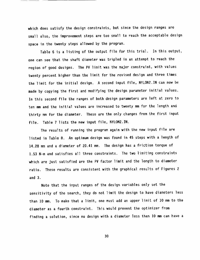
Table 6 is a listing of the output file for this trial. In this output,
one can see that the shaft diameter was tripled in an attempt to reach the
region of good designs. The PV limit was the major constraint, with values
twenty percent higher than the limit for the revised design and three times
the limit for the initial design. A second input file, NYLON2.1N can now be
made by copying the first and modifying the design parameter initial values.
In this second file the ranges of both design parameters are left at zero to
ten mm and the initial values are increased to twenty mm for the length and
thirty mm for the diameter. These are the only changes from the first input
file. Table 7 lists the new input file, NYLON2.1N.
The results of running the program again with the new input file are
listed in Table 8. An optimum design was found in 45 steps with a length of
14.28 mm and a diameter of 20.4] mm. The design has a friction torque of
1.53 N-m and satisfies all three constraints. The two limiting constraints
which are just satisfied are the PV factor limit and the length to diameter
ratio. These results are consistent with the graphical results of Figures 2
and 3.
Note that the input ranges of the design variables only set the
sensitivity of the search, they do not limit the design to have diameters less
than 10 mm. To make that a limit, one must add an upper limit of 10 mm to the
diameter as a fourth constraint. This would prevent the optimizer from
finding a solution, since no design with a diameter less than 10 mm can have a
30
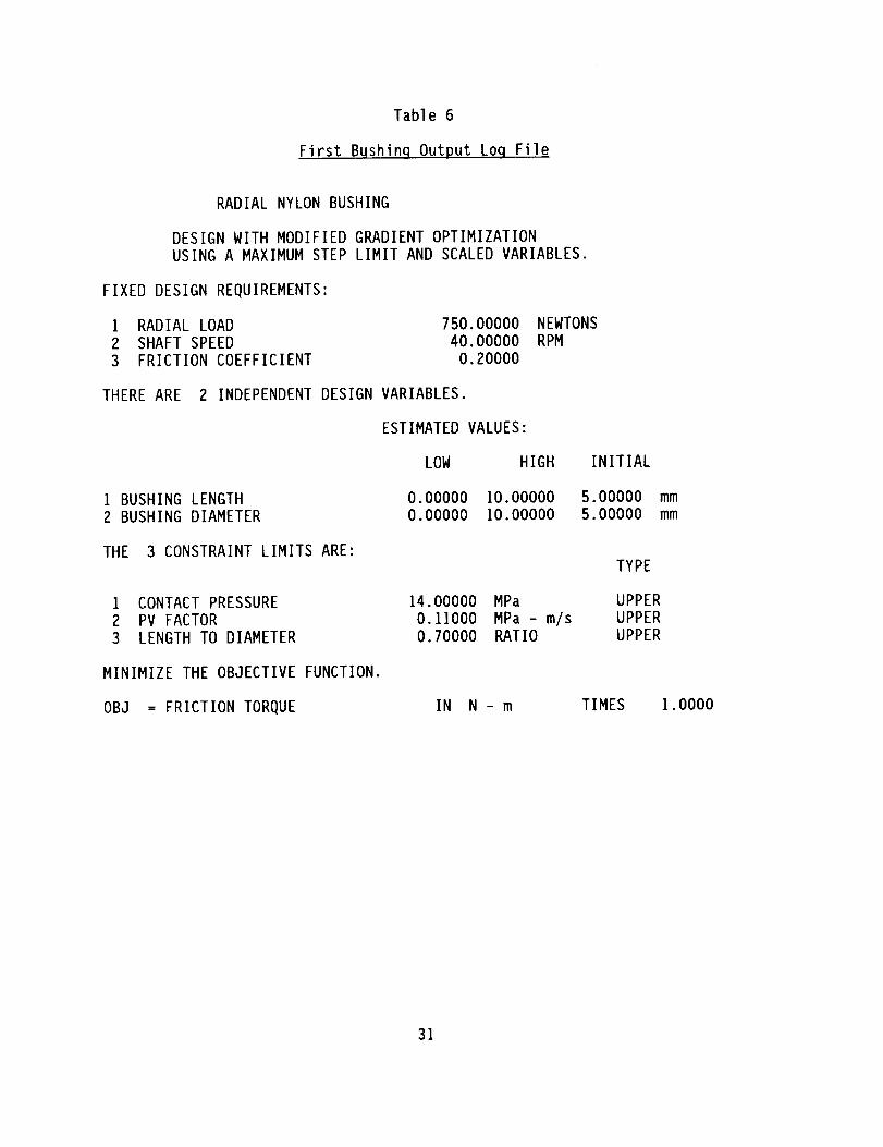
Table 6
First Bushinq Output Loq File
RADIAL NYLON BUSHING
DESIGN WITH MODIFIED GRADIENT OPTIMIZATION
USING A MAXIMUM STEP LIMIT AND SCALED VARIABLES.
FIXED DESIGN REQUIREMENTS:
I RADIAL LOAD 750.00000 NEWTONS
2 SHAFT SPEED 40.00000 RPM
3 FRICTION COEFFICIENT 0.20000
THERE ARE 2 INDEPENDENT DESIGN VARIABLES.
ESTIMATED VALUES:
LOW HIGH
I BUSHING LENGTH 0.00000 IO.O0000
2 BUSHING DIAMETER 0.00000 10.00000
THE 3 CONSTRAINT LIMITS ARE:
I CONTACT PRESSURE 14.00000 MPa
2 PV FACTOR 0.11000 MPa - m/s
3 LENGTH TO DIAMETER 0.70000 RATIO
MINIMIZE THE OBJECTIVE FUNCTION.
OBJ = FRICTION TORQUE IN N - m
INITIAL
5.00000 mm
5.00000 mm
TYPE
UPPER
UPPER
UPPER
TIMES 1.0000
31
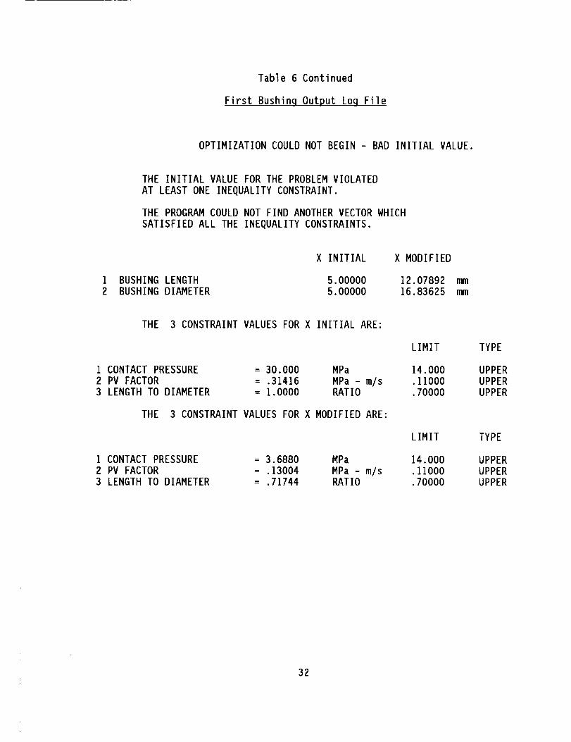
Table 6 Continued
First Bushinq Output Loq File
OPTIMIZATION COULD NOT BEGIN - BAD INITIAL VALUE.
THE INITIAL VALUE FOR THE PROBLEM VIOLATED
AT LEAST ONE INEQUALITY CONSTRAINT.
THE PROGRAM COULD NOT FIND ANOTHER VECTOR WHICH
SATISFIED ALL THE INEQUALITY CONSTRAINTS.
I BUSHING LENGTH2 BUSHING DIAMETER
X INITIAL X MODIFIED
5.00000 12.07892 mm
5.00000 16.83625 mm
THE 3 CONSTRAINT VALUES FOR X INITIAL ARE:
I CONTACT PRESSURE
2 PV FACTOR
3 LENGTH TO DIAMETER
= 30.000 MPa
= .31416 MPa - m/s= 1.0000 RATIO
THE 3 CONSTRAINT VALUES FOR X MODIFIED ARE:
] CONTACT PRESSURE
2 PV FACTOR
3 LENGTH TO DIAMETER
= 3.6880 MPa
= .13004 MPa - m/s= .71744 RATIO
LIMIT
14.000
.11000
.70000
LIMIT
14.000
.11000
.70000
TYPE
UPPERUPPER
UPPER
TYPE
UPPER
UPPER
UPPER
32

Table 7
Second Bushinq Input File
RADIAL NYLON BUSHING
3
750.0
RADIAL LOAD
NEWTONS
40.0
SHAFT SPEED
RPM
0.2
FRICTION COEFFICIENT
2
0.0 10.0 2O.O
BUSHING LENGTH
mm0.0 10.0 30.0BUSHING DIAMETER
mm3
UPPER 14.0
CONTACT PRESSURE
MPa
UPPER 0.11
PV FACTOR
MPa - m/sUPPER 0.7
LENGTH TO DIAMETER
RAT I0MIN
I
I.O
FRICTION TORQUEN - m
33

Table 8
Second Bushinq Output Locl File
RADIAL NYLON BUSHING
DESIGN WITH MODIFIED GRADIENT OPTIMIZATION
USING A MAXIMUM STEP LIMIT AND SCALED VARIABLES.
FIXED DESIGN REQUIREMENTS:
I RADIAL LOAD
2 SHAFT SPEED
3 FRICTION COEFFICIENT
THERE ARE
I BUSHING LENGTH
2 BUSHING DIAMETER
750.00000 NEWTONS
40.00000 RPM
0.20000
2 INDEPENDENT DESIGN VARIABLES.
ESTIMATED VALUES:
LOW HIGH
0.00000 10.000000.00000 10.00000
THE 3 CONSTRAINT LIMITS ARE:
1 CONTACT PRESSURE
2 PV FACTOR
3 LENGTH TO DIAMETER
MINIMIZE THE OBJECTIVE FUNCTION.
OBJ = FRICTION TORQUE
OPTIMIZATION SUCCESSFUL IN
THE FINAL DESIGN VECTOR IS:
14.00000 MPa
0.11000 MPa - m/s0.70000 RATIO
IN N - m
45 STEPS
x(1)
I BUSHING LENGTH 14.28342 mm
2 BUSHING DIAMETER 20.40649 mm
INITIAL
20.00000
30.00000
TYPE
UPPER
UPPER
UPPER
mm
mm
TIMES I.O000
THE MINIMUM OBJECTIVE FUNCTION = 1.53049 , ITS COMPONENTS ARE:
] FRICTION TORQUE = ].5305 N - m TIMES
THE LAST CHANGE IN THE OBJECTIVE FUNCTION = -0.677109E-04
THE LAST STEP CHANGE SIZE FOR THE DESIGN VARIABLE = 0.390625E-03
34
1.0000

Table 8 Continued
Second Bushinq Output Log File
THE 3 CONSTRAINT VALUES ARE:
I CONTACT PRESSURE
2 PV FACTOR
3 LENGTH TO DIAMETER
LIMIT TYPE
= 2.5735 MPa 14.000 UPPER
= .10999 MPa - m/s .11000 UPPER= .69989 RATIO .70000 UPPER
DESIGN CHECK
1 BUSHING LENGTH
2 BUSHING DIAMETER
X(1)
]5.00000 mm
21.00000 mm
THE MINIMUM OBJECTIVE FUNCTION = 1.57500
I FRICTION TORQUE = 1.5750
THE 3 CONSTRAINT VALUES ARE:
, ITS COMPONENTS ARE:
N - m TIMES I.O000
I CONTACT PRESSURE
2 PV FACTOR
3 LENGTH TO DIAMETER
LIMIT TYPE
= 2.3810 MPa ]4.000 UPPER
= .]0472 MPa - m/s .11000 UPPER= .71429 RATIO .70000 UPPER
DESIGN CHECK
i BUSHING LENGTH
2 BUSHING DIAMETER
X(1)
15.00000
22.00000mmmm
THE MINIMUM OBJECTIVE FUNCTION = 1.65000
I FRICTION TORQUE = 1.6500
THE 3 CONSTRAINT VALUES ARE:
1 CONTACT PRESSURE
2 PV FACTOR
3 LENGTH TO DIAMETER
= 2.2727
= .10472
= .68182
MPa
MPa - m/sRATIO
ITS COMPONENTS ARE:
N - m TIMES I.O000
LIMIT TYPE
14.000 UPPER
.11000 UPPER
.70000 UPPER
35

PV factor less than 0.11MPa - m/s and a B less than 0.7. Repeated trials
such as the first one would tell us that.
However, another constraint on the solution was that the diameter and
length be in whole mm's. This can be obtained with the design check provision
of the program, which is shown in Table 8. Once the numerical optimum has
been found, the program lists the number of optimizing steps followed by: the
found design parameter values for bushing length and bushing diameter, the
objective function value and the three constrained variable values and limits.
Then the program re-lists the design variables with their found values and
offers the user the option to change them for a design check. Figure 5 shows
this interaction. The user responded with a 'Y' to the question on trying
another design and entered the two values of '15' and '21' for the bushing
length and diameter. The program then printed the results to the screen and
added them to the output file as shown in Table 8. This option is offered to
the user at the end of each analysis until the response to the first question
is 'N' which tells the program to close the output file and stop the program.
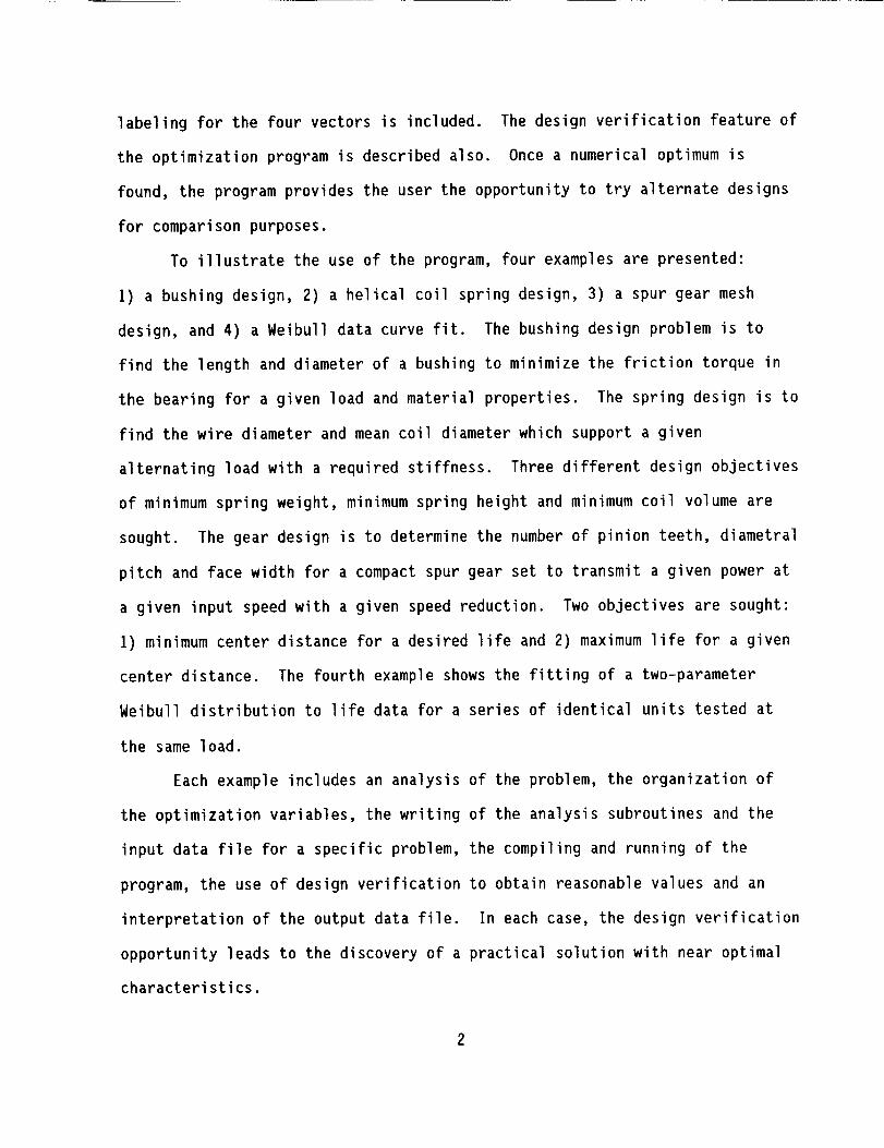
Increasing the length to 15 mm and the diameter to 21 mm increases the
friction torque slightly to 1.575 N-m but still does not satisfy the length to
diameter constraint. A second trial with a 15 mm length and a 22 mm diameter
has a friction torque of 1.65 mm and satisfies all three modeled constraints
and the additional requirement of standard sizes. This trial is the optimal
design and is shown in Figure 6.
36

I5
21
FORTHELASTDESIGN,THEDESIGNVARIABLEVECTORIS:
X(1)
BUSHINGLENGTH 14.28342 mmBUSHINGDIAMETER 20.40649 mm
DOYOUWISHTOMODIFYTHEDESIGNANDCHECKIT ? (Y/N)
ENTERNEWVALUESFORTHEDESIGNVARIABLEVECTOR,X.ENTERA COMMA"," TOKEEPTHISVALUE.
OLDBUSHINGLENGTHNEWBUSHINGLENGTH =?
14.28342 mm
OLDBUSHINGDIAMETERNEWBUSHINGDIAMETER =?
20.40649 mm
Seek Design Verification Request Screen
FIGURE 5
37

E
5L_
..J
o_1
)
c-o'_
-- 13_
ZI:EZ..OO
.-I .,_- i._.. P,,.
ryn ..wWr'_I-- m _:"_: O-. O"_0_/
ZCD
O0m
CDZ _D
I W
O0 C__
F--0_0
38

SPRINGOPTIMIZATION
In this example, consider the design of a steel helical coil compression
spring to support a varying load with a specified spring rate. The applied
load varies betweenminimumand maximumvalues in service and may be larger if
the spring is compressedsolid at assembly. For a given spring material, four
geometric parameters define the spring: I) the wire diameter, dw; 2) the mean
coil diameter, D; 3) the numberof active coils, Na; and 4) the height of the
spring when unloaded, hf.
In this design problem, one more requirement can be placed on the
performance of the spring: it could have a specified outside diameter, or work
over a rod of a given diameter or it could have a required height under load.
Instead, we will let the optimizer find a spring with a minimized property
which can support the specified loads with the given spring rate. Three
separate objective functions will be minimized: I) spring weight, 2) spring
height, and 3) spring coil volume. The resulting designs will satisfy the
load and deflection requirements, but they will be different.
For the spring design to have somepracticality, the wire size should be
selected from a finite list of available diameters and the meancoil diameter
should also be a standard size.
Theor_
A spring's performance is modeled by its strength and deflection. A
helical coil spring supports its axial load as a torsional shear stress in the
wire with a small additional direct shear stress. Figure 7 shows the axial
load and the internal wire torque and shear which support it. Due to the
curvature of the wire, Wahl determined a stress concentration factor, Kw,
which compares the maximumshear stress in the wire to the nominal torsional
39

F
d w
_L
V
INTERNAL LOADS
SHEAR STRESSES
HELICAL COIL SHEAR LOADS AND STRESSES
FIGURE 7
4O
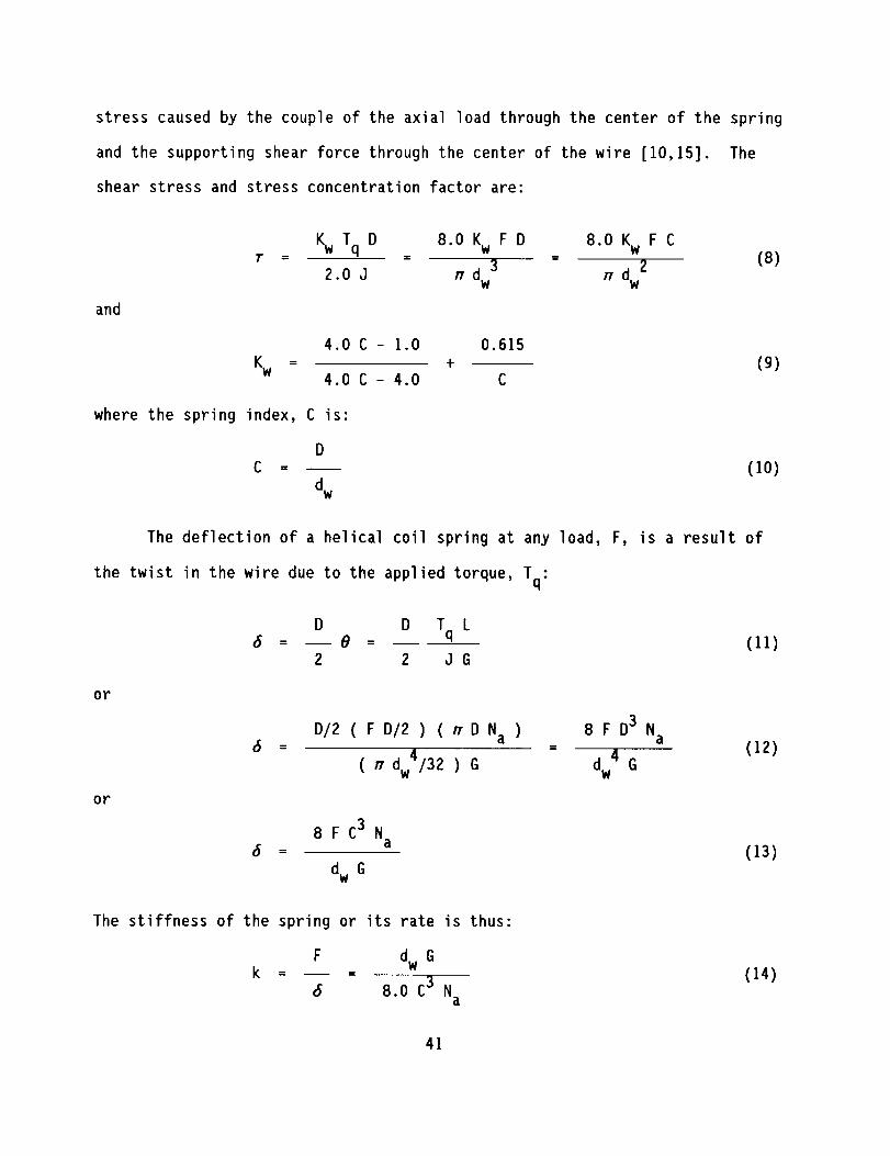
stress caused by the couple of the axial load through the center of the spring
and the supporting shear force through the center of the wire [I0,15]. The
shear stress and stress concentration factor are:
Kw Tq D 8.0 Kw F D 8.0 Kw F C
r - - dw3 - 2 (8)2.0 J u ud w
and
4.0 C - 1.0 0.615
Kw = + (g)4.0 C - 4.0 C
where the spring index, C is:
D
C -
dw
(10)
The deflection of a helical coil spring at any load, F, is a result of
the twist in the wire due to the applied torque, T :q
or
or
D D T L
6 - 0 - q (11)2 2 JG
D/2 ( F D/2 ) ( u D Na ) 8 F D3 Na6 = (12)
( u dw4/32 ) G dw4 G
8 F C3 Na6 = (13)
dw G
The stiffness of the spring or its rate is thus:
F dw Gk - - (14)
6 8.0 C3 Na
41
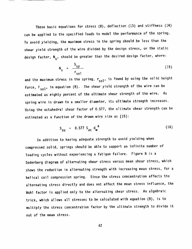
These basic equations for stress (8), deflection (13) and stiffness (14)
can be applied to the specified loads to model the performance of the spring.
To avoid yielding, the maximumstress in the spring should be less than the
shear yield strength of the wire divided by the design stress, or the static
design factor, Ns, should be greater than the desired design factor, where:
Ns - Ssy (15)rsol
and the maximum stress in the spring, rso l, is found by using the solid height
force, Fso l, in equation (8). The shear yield strength of the wire can be
estimated as eighty percent of the ultimate shear strength of the wire. As
spring wire is drawn to a smaller diameter, its ultimate strength increases.
Using the octahedral shear factor of 0.577, the ultimate shear strength can be
estimated as a function of the drawn wire size as [15]:
Ssu = 0.577 Suc dwa (16)
In addition to having adequate strength to avoid yielding when
compressed solid, springs should be able to support an infinite number of
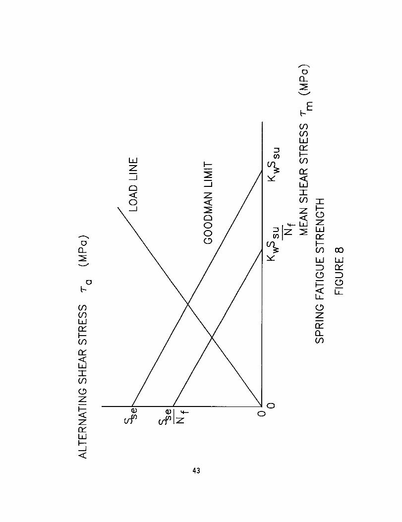
loading cycles without experiencing a fatigue failure. Figure 8 is a
Soderberg diagram of alternating shear stress versus mean shear stress, which
shows the reduction in alternating strength with increasing mean stress, for a
helical coil compression spring. Since the stress concentration affects the
alternating stress directly and does not affect the mean stress influence, the
Wahl factor is applied only to the alternating shear stress. An algebraic
trick, which allows all stresses to be calculated with equation (8), is to
multiply the stress concentration factor by the ultimate strength to divide it
out of the mean stress.
42
o0_
w0_
O9
<wS
(_9Z
<Z
WF-__J<
43
On
V
Et--
O0O9LLJ
CA
I
Z<
%
00
IF-
ZW0_
cO
Ld Wr_
LD
D_
CDZ
r_0_

In Figure 8, the negative sloped lines show the Goodman criteria for
fatigue strength with and without the design factor, Nf, and the positive
sloped line shows the load ratio of alternating stress, ra, to mean stress,
rm, for this application.
[is]:1
Nf
The design factor equation for this criteria is
r m r a+ (17)
Kw Ssu Sse
or
1.0
Nf = (18)Tm r a
+
Kw Ssu Sse
The mean stress is calculated with equation (8) using the average applied
load:
Fmax + Fmin
Fm = (19)2.0
And the alternating stress is calculated using the alternating applied load:
Fmax - Fmin
Fa = (20)2.0
Unlike the ultimate wire strength, the fatigue strength of the steel wire,
Sse, is constant at these high strengths.
Figure g is a plot of the force on the spring versus the height of the
spring. Near the solid height, the axial load on the spring increases rapidly
as the coils close. In service, the spring operates between the working
heights of hmi n and hma x with loads of Fmax and Fmin, The unloaded height of
the spring is the sum of the deflection to solid height and the solid height:
44

AXIAL LOAD - F (,N)
Fsolid
Fmax
Frain
0
WORKING___HEIGHT
II
k
0 hsolid h min h mox h f
SPRING HEIGHT- h (mm)
SPRING FORCE VERSUS
FIGURE 9
POSITION
45

hf
Fsolm
k+ 1.0] dw ( Na + Ne ) (21)
Coil weight is a direct function of the volume of wire in the spring:
/7
Vw - dw2 ( Na + Ne ) n D4
with:
(22)
Wt = w Vw (23)
The volume of the coil is the area of the outside diameter's circular disc
times the spring height:
Vcoil - OD 2 hf (24)4
Proqramminq
Table 9 summarizes the design problem in terms of the constants which
define the problem, the design parameters which are to be found, the equality
and inequality constraints on the design and the three separate objective
functions which will be sought. In the initial formulation, there are two
equality constraints on the stiffness and the force at solid height, which can
be used to reduce the number of independent design parameters from four to
two. There are four active inequality constraints: I) that the number of
active coils be positive, 2) that the fatigue design factor be greater than
the desired design factor, 3) that the static design factor at assembly be
greater than the desired design factor, and 4) that the spring index be
greater than two, so a coil can be manufactured.
46

Table 9
Initial Sprinq Optimization Parameters
Constants
Fmin
Fmax
Fsolid
k
Ne
Ndes
Sse
SSU
G
W
Design
d w
D
Na
hf
Constraints
Equality Inequality
Na > 0.0
Nf > Nde s
Ns > Nde s
C >2.0
Parameters
k
Fsolid
Objective Function
(hf)min
or
(Wt)mi n
or
(VOl)mi n
Table 10
Revised Sprinq Optimization Parameters
Constants Design Parameters Inequality Constraints Objective Function
Fmin
Fmax
Fsolid
k
Ne
Sse
Suc
a
G
W
d w
D
Na>O.O
Nf > Nde s
Ns > Nde s
C >2.0
rmax>O.O
OD>O.O
Vw>O.O
(hf)mi n
or
(Wt)min
or
(Vol)min
47

From the stiffness equation (I4), one can relate the numberof active
coils to the wire and meancoil diameters, the stiffness and the shear modulus
of the material:
dw G
Na - (25)8.0 k C3
Equation (2]) relates the spring height to: the maximum force, Fsol; the
spring rate; the wire diameter; and the numbers of active and end coils.
These two equations convert two design parameters from independent parameters
to dependent parameters and simplify the optimization. Table 10 is a second
pass at formulating the optimization problem in this simpler form. Three
inactive constraints have been added to the inequality constraint list to make
the optimizer report these properties. All properties are constrained to be
greater than zero, which they will be for all designs. The watched properties
are: 1) maximum static stress, Tmax; 2) outside diameter, OD; and 3) wire
volume, Vw. The final differences between the two formulations are in the
constant list: I) the elimination of the design factor from the constant list
since it is used in the constraint limit list and, 2) the replacement of the
ultimate shear strength of the wire by the ultimate tensile strength constant
and the wire power to enable the program to vary the strengths with wire size.
Figure 10 is a plot of the design space for this reformulated
optimization. The graph plots the two independent design parameters: the wire
diameter, dw, and the mean coil diameter, D, versus each other. On the graph
are drawn constraint lines for the four active constraints. The number of
active coils constraint, Na, is drawn for a limit of 0.1 coils to show its
shape. A limit of zero coils lies on the x axis. Designs which satisfy all
48

o o
Z
o
0
W(.)
clU'l
Z
0'3i,IC3
Z
13..
...A
OO
.__1
(D_Akl_lT
O
WC12_D
49
constraints can be found in the region labeled acceptable designs which is
between the spring index limit, labeled C, and the solid stress limit, labeled
SOLID.
Each of the three objective functions are complex functions of these
parameters, so a single plot of the objective function versus mean coil
diameter is not possible. Contour plots for each objective function would
have to be drawn on the design space to obtain a graphical solution to the
problem.
Two analysis subroutines must now be written to operate on the constants
and design parameters of Table 10 and determine the constraint values and the
objective function values listed. Subroutine BOUNDS, which is listed in
Table 11, takes the constant array and the design parameter array from the
calling list and determines the constraint values. As with the bushing
example, this is done in three steps to clarify the calculations:
]) conversion of input arrays to variables, 2) calculation of the properties
and 3) transferring the property values to the constraint property array. The
analysis of equations (8) through (25) is used in the subroutine. Subroutine
VALUES, which is listed in Table 12, performs a similar determination of the
three objective function values. Once written, these two subroutines must be
compiled and linked to program SEEK to generate an executable program to
perform the optimization.
Numerical Example
For the example, consider the design of a spring to have a spring rate
of 4 kN/m. In use, the spring will see a load which varies from a minimum of
24 N to a maximum of 120 N. The spring should not go solid until the applied
load reaches a value of 150 N. The spring wire is to be selected from stock
50

Table 11
Sprinq Constraint Evaluation Subroutine Bounds
C
C
C
C
C
C
C
C
C
C
C
C
C
C
C
C
C
C
C
C
C
CC
C
CC
C
C
C
C
C
C
CC
C
C
C
CC
C
SUBROUTINE BOUNDS(CONST,NCO,X,NX,VCSTR,NCS)
BOUNDS DETERMINES THE PRESENT CONSTRAINT
FUNCTION VALUES
FOR A HELICAL COIL SPRING DESIGN
PARAMETERS:
CONST - FIXED DESIGN CONSTANT
NCO - NUMBER OF DESIGN CONSTANTS
NCS - NUMBER OF INEQUALITY CONSTRAINTSNX - NUMBER OF INDEPENDENT DESIGN VARIABLES
VCSTR - PRESENT CONSTRAINT VALUESX - PRESENT DESIGN VARIABLE VALUES
ALL VALUES ARE IN PROBLEM UNITS
CONST(1) = Fmin
CONST(2) = Fmax
CONST(3) = Fsol
CONST(4) = k
CONST(5) = Ne
CONST(6) = Sse
CONST(7) = Suc
CONST(8) = a
CONST(9) = GCONST(IO) = w
- MINIMUM FORCE (NEWTONS)
- MAXIMUM FORCE (NEWTONS)
- MINIMUM SOLID FORCE (NEWTONS)
- SPRING RATE (kN/m)- NUMBER OF DEAD COILS
- SHEAR FATIGUE STRENGTH (MPa)
- TENSILE STRENGTH COEFICIENT (MPa)- TENSILE STRENGTH WIRE POWER
- SHEAR MODULUS (MPa)
- WEIGHT DENSITY (kN/m**3)
x(1) = dwX(2) = D
- WIRE DIAMETER (mm)- MEAN COIL DIAMETER (mm)
VCSTR(1) = Na
VCSTR(2) = Nf
VCSTR(3) = Ns
VCSTR(4) = CVCSTR(5) = Tmax
VCSTR(6) = OD
VCSTR(7) = Vw
- NUMBER OF ACTIVE COILS
- FATIGUE DESIGN FACTOR
- STATIC DESIGN FACTOR
- SPRING INDEX
- MAXIMUM SHEAR STRESS (MPa)
- OUTSIDE DIAMETER (mm)
- SPRING WIRE VOLUME (mm**3)
51

Table 11 Continued
Sprinq Constraint Evaluation Subroutine Bounds
C
DIMENSION CONST(NCO),X(NX),VCSTR(NCS)
PI = 3.]4]59265
FMIN = CONST(1)
FMAX = CONST(2)
FSOL = CONST(3)
RATE = CONST(4)
ZNE = CONST(5)SSE = CONST(6)
CSUT = CONST(7)
ASUT = CONST(8)
G = CONST(9)DW = X(1)
D = X(2)
C = D/DW
ZNA = DW*G/(B.O*C*C*C*RATE)SSU = 0.577 * CSUT * DW**ASUT
SSY = O.8*SSU
FA = (FMAX - FMIN)/2.0
FM = (FMAX + FMIN)/2.0SKW = (4.0"C - ].0)/(4.0"C - 4.0) + 0.615/C
TA = (8.0*SKW*FA*C/(PI*DW*DW))
TM = (8.0*FM*C/(PI*DW*DW))
ZNF = 1.0/(TM/SSU + TA/SSE)
TMAX = (8.0*SKW*FSOL*C/(PI*DW*DW))
ZNS = SSY/TMAXOD = D + DW
ZNT = ZNA + ZNEVW = O.25*PI*DW*DW*ZNT*PI*D
VCSTR(1) = ZNAVCSTR(2) = ZNF
VCSTR(3) = ZNS
VCSTR(4) = C
VCSTR(5) = TMAX
VCSTR(6) = OD
VCSTR(7) = VWRETURN
END
52

Table 12
Sprinq Objective Function Evaluation Subroutine Values
C
CC
C
C
C
C
C
C
C
C
C
C
C
C
C
C
C
C
C
C
C
C
C
C
C
C
C
CC
C
C
C
C
C
C
SUBROUTINE VALUES(CONST,NCO,X,NX,OBJECT,NOB)
VALUES DETERMINES THE PRESENT DESIGN
OBJECTIVE FUNCTION VALUES
FOR A CANTILEVER BEAM DESIGN EXAMPLE
PARAMETERS:
CONST - FIXED DESIGN CONSTANT
NCO - NUMBER OF DESIGN CONSTANTS
NOB - NUMBER OF OBJECTIVE FUNCTION TERMS
NX - NUMBER OF INDEPENDENT DESIGN VARIABLES
OBJECT - PRESENT OBJECTIVE FUNCTION VALUES
X - PRESENT DESIGN VARIABLE VALUES
ALL VALUES ARE IN PROBLEM UNITS
CONST(I) = Fmin
CONST(2) = Fmax
CONST(3) = Fsol
CONST(4) = k
CONST(5) = Ne
CONST(6) = SseCONST(7) = Suc
CONST(8) = a
CONST(9) = G
CONST(IO) = w
- MINIMUM FORCE (NEWTONS)
- MAXIMUM FORCE (NEWTONS)
- MINIMUM SOLID FORCE (NEWTONS)
- SPRING RATE (kN/m)- NUMBER OF DEAD COILS
- SHEAR FATIGUE STRENGTH (MPa)
- TENSILE STRENGTH COEFICIENT (MPa)- TENSILE STRENGTH WIRE POWER
- SHEAR MODULUS (MPa)
- WEIGHT DENSITY (kN/m**3)
x(1) = dwX(2) = D
- WIRE DIAMETER (mm)- MEAN COIL DIAMETER (mm)
OBJECT(1) = Wt
OBJECT(2) = hf
OBJECT(3) = Vc
- SPRING WEIGHT (NEWTONS)
- SPRING HEIGHT (mm)
- SPRING CYLINDER VOLUME (mm**3)
DIMENSION CONST(NCO),X(NX),OBJECT(NOB)PI = 3.14159265
FSOL = CONST(3)
RATE = CONST(4)
ZNE = CONST(5)
G = CONST(9)
W = CONST(IO)/IO00000.O
53

Table 12 Continued
Sprinq Objective Function Evaluation Subroutine Values
C
DSOL = FSOL/RATE
DW = X(1)D = X(2)
C = D/DWOD = D + DW
ZNA = DW*G/(B.O*C*C*C*RATE)ZNT = ZNA + ZNE
VW = O.25*PI*DW*DW*ZNT*PI*D
WT = VW*W
HF = DSOL + DW*ZNT*I.01
VC = O.25*PI*OD*OD*HF
OBJECT(1) = WT
OBJECT(2) = HF
OBJECT(3) = VCRETURNEND
54
sizes which have whole and half mmvalues. The meancoil diameter should also
have values with whole or half mmprecision. The springs are to be madeof
hard drawn spring wire with an ultimate strength constant of ]5]0 MPa, a wire
diameter strength variation exponent of -0.201, and a shear fatigue strength
of 465 MPa. The acceptable design factor is 1.5 and the spring ends are to be
squared and ground with one inactive coil at each end. The shear modulus of
steel is 79,000 MPaand its weight density is 76.5 kN/m3.
Table 13 is a listing of the input file for the minimumweight design
option. The file begins with the title for the output file. The second line
has the numberof constants to follow - ten. The next thirty lines contain
these ten constants in the order listed in Table 10 with their descriptions
and units. Following the constants is a line with the number two which
indicates that two independent design parameters will follow. These two
parameters are the wire diameter and the meancoil diameter. Low, high and
initial estimates are selected as 1.0, 15.0 and 5.0 for the wire size and
25.0, 500.0 and 100.0 for the meancoil diameter. The next line has the
single value of seven for the seven design constraints listed in Table 10.
All seven constraints happento be lower. Following the constraints is a line
with the letters 'MIN' to select minimization as the direction of
optimization, a line with the value of three to indicate that there are three
terms in the objective function. The last nine lines are the weighting
coefficients, names and units for the three objective function terms of
weight, height and volume. The weighting coefficient of the first is one and
the last two are zero. By changing which term has the unit coefficient, one
can change the optimization goal without changing the program.
55

Table 13
Sprinq Desiqn Input File For Minimum Weiqht
HELICAL COIL SPRING - MINIMUM WEIGHT
I0
24.0
MINIMUM FORCE
NEWTONS
120.0MAXIMUM FORCE
NEWTONS
150.0MINIMUM FORCE WHEN SOLID
NEWTONS
4.0
SPRING RATE
kN/m2END COIL NO.
465.0
SHEAR FATIGUE STRENGTH
MPa
1510.0
TENSILE STRENGTH CONSTANT
MPa
-0.201
TENSILE STRENGTH WIRE POWER
79000.0
SHEAR MODULUS
MPa
76.5
WEIGHT DENSITY
kN/m**32
1.0 15.0 5.0
WIRE DIAMETER
mm25.0 500.0 100.0
MEAN COIL DIAMETER
mm
56

Table 13 Continued
Sprinq Desiqn Input File For Minimum Weiqht
7
LOWER 0.0
ACTIVE COIL
NO.LOWER 1.5
FATIGUE DESIGN FACTOR
LOWER 1.5
STATIC DESIGN FACTOR
LOWER 2.0
SPRING INDEX
LOWER O. 0
MAXIMUM SHEAR STRESS
MPa
LOWER O. 0
OUTSIDE COIL DIAMETER
mmLOWER O. 0
SPRING WIRE VOLUME
mm**3
MIN
3].0
WEIGHT
NEWTONS
0.0HEIGHT
mm0.0
SPRING COIL VOLUME
mm**3
57

This ASCII file can then be saved with a namesuch as 'WEIGHT.IN' and
used with the spring optimization program. Table 14 is the output file which
resulted from running the spring optimization program with this file. The ten
constants, two design parameters, seven constraints and three objective
function term are all listed with their values, names, units, limit
directions, and weighting coefficients at the start of the file. The
optimization reached a solution in 24 steps with a wire diameter of slightly
more than 3 mmand a meancoil diameter of 23.13 mm. The spring weight was
0.79 Newtons and the spring had 17.5 active coils with a height of 97 mma
spring index of 7.5 and a spring coil volume of 52,000 mm3. The static
overload stress was the limiting factor in the design with a static design
factor of 1.5 at the limit and a maximumshear stress of 370 MPa.
Following this output is a design check with a 3.5 mmwire diameter and
a meancoil diameter of 35 mm. With the larger standard wire size, the larger
coil diameter keeps the spring weight downby reducing the numberof active
coils needed to obtain the spring rate without lowering the design factors.
The weight increased to 0.86 Newtons, the numberof active coils dropped to
8.64 and the spring index increased to 10. In addition, the height dropped to
75 mmand the spring coil volume increased to 87,500 mm3. Although the spring
is slightly heavier than the initial optimum, it has standard wire and coil
dimensions, so it is a practical optimal solution to the posed problem.
Table 15 is the output file produced by running the spring optimization
program with a second input file which has two weighting coefficients changed
and the problem title changed in line one. The two numerical changes were to
the first and second weighting coefficient values to switch the object of
minimization from weight to height. As shownin Table 15, this optimum is
58

Table 14
Sprinq Desiqn Output File For Minimum Weiqht
HELICAL COIL SPRING - MINIMUM WEIGHT
DESIGN WITH MODIFIED GRADIENT OPTIMIZATION
USING A MAXIMUM STEP LIMIT AND SCALED VARIABLES.
FIXED DESIGN REQUIREMENTS:
I MINIMUM FORCE
2 MAXIMUM FORCE
3 MINIMUM FORCE WHEN SOLID
4 SPRING RATE5 END COIL NO.
6 SHEAR FATIGUE STRENGTH
7 TENSILE STRENGTH CONSTANT
8 TENSILE STRENGTH WIRE POWER
9 SHEAR MODULUS
10 WEIGHT DENSITY
24.00000 NEWTONS
120.00000 NEWTONS
150.00000 NEWTONS
4.00000 kN/m2.00000
465.00000 MPa
1510.00000 MPa
-0.20100
79000.00000 MPa
76.50000 kN/m**3
THERE ARE 2 INDEPENDENT DESIGN VARIABLES.
ESTIMATED VALUES:
LOW HIGH INITIAL
I WIRE DIAMETER
2 MEAN COIL DIAMETER
1.00000 15.00000 5.00000 mm
25.00000 500.00000 100.00000 mm
THE 7 CONSTRAINT LIMITS ARE:
I ACTIVE COIL
2 FATIGUE DESIGN FACTOR
3 STATIC DESIGN FACTOR
4 SPRING INDEX
5 MAXIMUM SHEAR STRESS
6 OUTSIDE COIL DIAMETER
7 SPRING WIRE VOLUME
0.00000 NO.
1.50000
1.500002.00000
0.00000 MPa
0.00000 mm
0.00000 mm**3
MINIMIZE THE OBJECTIVE FUNCTION, WHICH HAS 3 TERMS.
OBJ = THE LINEAR SUM OF:
1 WEIGHT IN NEWTONS TIMES
2 HEIGHT IN mm TIMES
3 SPRING COIL VOLUME IN mm**3 TIMES
TYPE
LOWER
LOWER
LOWER
LOWERLOWER
LOWER
LOWER
1.0000
0.0000
0.0000
59

Table 14 Continued
Sprinq Design Output File For Minimum Weiqht
OPTIMIZATION SUCCESSFUL IN
THE FINAL DESIGN VECTOR IS:
24 STEPS
X(1)
1 WIRE DIAMETER 3.05491 mm2 MEAN COIL DIAMETER 23.12969 mm
THE MINIMUM OBJECTIVE FUNCTION = 0.789480 ITS COMPONENTS ARE:
I WEIGHT =0.78948 NEWTONS TIMES
2 HEIGHT = 97.285 mm TIMES
3 SPRING COIL VOLUME = 52388. mm**3 TIMES
1.00000.00000.0000
THE LAST CHANGE IN THE OBJECTIVE FUNCTION = 0.596046E-07THE LAST STEP CHANGE SIZE FOR THE DESIGN VARIABLE = 0.390625E-03
THE 7 CONSTRAINT VALUES ARE:
I ACTIVE COIL
2 FATIGUE DESIGN FACTOR
3 STATIC DESIGN FACTOR
4 SPRING INDEX
5 MAXIMUM SHEAR STRESS
6 OUTSIDE COIL DIAMETER
7 SPRING WIRE VOLUME
LIMIT
= 17.525 NO. .00000
= 2.1345 1.5000
= ].5035 ].5000
= 7.5462 2.0000
= 370.49 MPa .00000
= 26.070 mm .00000
= 10320. mm**3 .00000
TYPE
LOWER
LOWERLOWER
LOWER
LOWER
LOWER
LOWER
60

Table 14 Continued
Sprinq Desiqn Output File For Minimum Weiqht
DESIGN CHECK
] WIRE DIAMETER
2 MEAN COIL DIAMETER
X(1)
3.50000 mm
35.00000 mm
THE MINIMUM OBJECTIVE FUNCTION =
I WEIGHT
2 HEIGHT
3 SPRING COIL VOLUME
0.861137 , ITS COMPONENTS ARE:
=0.86114 NEWTONS TIMES
= 75.115 mm TIMES
= 87445. mm**3 TIMES
THE 7 CONSTRAINT VALUES ARE:
I ACTIVE COIL
2 FATIGUE DESIGN FACTOR
3 STATIC DESIGN FACTOR
4 SPRING INDEX
5 MAXIMUM SHEAR STRESS6 OUTSIDE COIL DIAMETER
7 SPRING WIRE VOLUME
= 8.6406
= 2.1430
= ].5179
= ]0.000
= 356.97
= 38.500
= 11257.
NO.
MPa
mmmm**3
LIMIT
.00000
1.5000
1.5000
2.0000
.00000
.00000
.00000
l.O000
0.00000.0000
TYPE
LOWER
LOWER
LOWER
LOWER
LOWER
LOWER
LOWER
61

Table 15
Sprinq Desiqn Output File For Minimum Height
HELICAL COIL SPRING - MINIMUM HEIGHT
DESIGN WITH MODIFIED GRADIENT OPTIMIZATION
USING A MAXIMUM STEP LIMIT AND SCALED VARIABLES.
FIXED DESIGN REQUIREMENTS:
I MINIMUM FORCE
2 MAXIMUM FORCE
3 MINIMUM FORCE WHEN SOLID
4 SPRING RATE
5 END COIL NO.
6 SHEAR FATIGUE STRENGTH7 TENSILE STRENGTH CONSTANT
8 TENSILE STRENGTH WIRE POWER
9 SHEAR MODULUS
10 WEIGHT DENSITY
24.00000 NEWTONS
120.00000 NEWTONS
150.00000 NEWTONS
4.00000 kN/m2.00000
465.00000 MPa
1510.00000 MPa
-0.20100
79000.00000 MPa
76.50000 kN/m**3
THERE ARE 2 INDEPENDENT DESIGN VARIABLES.
ESTIMATED VALUES:
LOW HIGH INITIAL
I WIRE DIAMETER
2 MEAN COIL DIAMETER
I.O0000 15.00000 5.00000 mm
25.00000 500.00000 100.00000 mm
THE 7 CONSTRAINT LIMITS ARE:
! ACTIVE COIL
2 FATIGUE DESIGN FACTOR
3 STATIC DESIGN FACTOR
4 SPRING INDEX
5 MAXIMUM SHEAR STRESS
6 OUTSIDE COIL DIAMETER
7 SPRING WIRE VOLUME
0.00000 NO.
1.50000
1.50000
2.00000
0.00000 MPa
0.00000 mm
0.00000 mm**3
MINIMIZE THE OBJECTIVE FUNCTION, WHICH HAS 3 TERMS.
OBJ = THE LINEAR SUM OF:
I WEIGHT IN NEWTONS TIMES
2 HEIGHT IN mm TIMES
3 SPRING COIL VOLUME IN mm**3 TIMES
TYPE
LOWER
LOWER
LOWER
LOWER
LOWER
LOWER
LOWER
0.0000
1.0000
0.0000
62

Table 15 Continued
Sprinq Desiqn Output File For Minimum Heiqht
OPTIMIZATION SUCCESSFUL IN
THE FINAL DESIGN VECTOR IS:
14 STEPS
x(1)
I WIRE DIAMETER 6.30577 mm
2 MEAN COIL DIAMETER 195.96942 mm
THE MINIMUM OBJECTIVE FUNCTION = 53.5408 , ITS COMPONENTS ARE:
1 WEIGHT = 3.7045 NEWTONS TIMES
2 HEIGHT = 53.541 mm TIMES
3 SPRING COIL VOLUME =0.17205E+07 mm**3 TIMES
0.00001.00000.0000
THE LAST CHANGE IN THE OBJECTIVE FUNCTION = 0.381470E-04
THE LAST STEP CHANGE SIZE FOR THE DESIGN VARIABLE = 0.625000E-02
THE 7 CONSTRAINT VALUES ARE:
I ACTIVE COIL
2 FATIGUE DESIGN FACTOR
3 STATIC DESIGN FACTOR
4 SPRING INDEX
5 MAXIMUM SHEAR STRESS
6 OUTSIDE COIL DIAMETER
7 SPRING WIRE VOLUME
LIMIT
= .53093 NO. .00000= 2.2086 1.5000
= 1.5438 1.5000
= 30.786 2.0000
= 312.12 MPa .00000
= 199.46 mm .00000
= 47506. mm**3 .00000
TYPE
LOWER
LOWER
LOWER
LOWER
LOWER
LOWER
LOWER
63
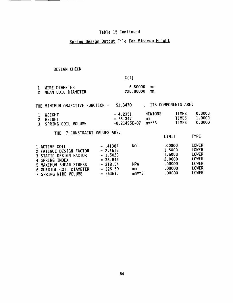
Table 15 Continued
Sprinq Desiqn Output File For Minimum Heiqht
DESIGN CHECK
I WIRE DIAMETER
2 MEAN COIL DIAMETER
X(1)
6.50000
220.00000mm
mm
THE MINIMUM OBJECTIVE FUNCTION =
I WEIGHT
2 HEIGHT
3 SPRING COIL VOLUME
53.3470 , ITS COMPONENTS ARE:
= 4.2351 NEWTONS
= 53.347 mm
=0.21495E+07 mm**3
THE 7 CONSTRAINT VALUES ARE:
= .41387
= 2.1515
= 1.5020
= 33.846
= 318.54
= 226.50
= 55361.
I ACTIVE COIL
2 FATIGUE DESIGN FACTOR
3 STATIC DESIGN FACTOR
4 SPRING INDEX
5 MAXIMUM SHEAR STRESS
6 OUTSIDE COIL DIAMETER
7 SPRING WIRE VOLUME
TIMES
TIMES
TIMES
NO.
MPa
im
mm**3
LIMIT
.00000
1.5000
1.5000
2.0000
.00000
.00000
.00000
0.0000
1.0000
0.0000
TYPE
LOWER
LOWER
LOWER
LOWER
LOWER
LOWER
LOWER
64

different from the first. The spring has a wire diameter of 6.3 mmand a mean
coil diameter of 196 mmwith only 0.53 active coils and a spring index of 31.
The height is shorter at 53.5 mmbut the weight is higher at 3.7 Newtons and
the spring coil volume is muchhigher at 1.72"106 mm3. This design was also
limited by the static design factor.
However, it was reached in only 14 trials and the static design factor
was slightly higher than 1.5 at 1.54. These two facts indicate that this may
not be an absolute minimumheight design. Changing the starting position as
was done for the bushing design or changing the sensitivity ranges on the two
independent design parameters would give the optimizer a chance to search
longer and find a slightly better optimal design. However, since we were
going to change the wire size and meancoil diameter to standard values
anyway, the starting position and sensitivity ranges were not changed. The
design check chosen has a wire diameter of 6.5 mmand a meancoil diameter of
220 mmfor a height of 53.3 mm. This design is also heavy and large with a
fraction of an active coil at 0.41 and a spring index of 34.
Table 16 shows the output file for a design which minimizes the spring
coil volume. The only changes in the input file for this case were the
weighting coefficients in the objective function list to select spring volume
as the target for minimization and the problem title. This design was
achieved in 28 steps and has a wire diameter of 2.2 mmand a meancoil
diameter of 7.5 mm. The spring coil volume is the smallest of the found
designs at 26,300 mm3 which is about one-half that of the first design.
However it is heavier at 0.99 Newtonsand muchlonger at 355 mm. The spring
index is small at 3.4 and the numberof active coils is large at 140.
Changing the wire diameter to 2.5 mmand the meancoil diameter to 11.5 mm
65

Table 16
Sprinq Desiqn Output File For Minimum Coil Volume
HELICAL COIL SPRING - MINIMUM COIL VOLUME
DESIGN WITH MODIFIED GRADIENT OPTIMIZATION
USING A MAXIMUM STEP LIMIT AND SCALED VARIABLES.
FIXED DESIGN REQUIREMENTS:
I MINIMUM FORCE2 MAXIMUM FORCE
3 MINIMUM FORCE WHEN SOLID
4 SPRING RATE
5 END COIL NO.
6 SHEAR FATIGUE STRENGTH
7 TENSILE STRENGTH CONSTANT
8 TENSILE STRENGTH WIRE POWER
9 SHEAR MODULUS
10 WEIGHT DENSITY
24.00000 NEWTONS
120.00000 NEWTONS
150.00000 NEWTONS
4.00000 kN/m2.00000
465.00000 MPa
1510.00000 MPa
-0.20100
79000.00000 MPa
76.50000 kN/m**3
THERE ARE 2 INDEPENDENT DESIGN VARIABLES.
ESTIMATED VALUES:
LOW HIGH INITIAL
I WIRE DIAMETER2 MEAN COIL DIAMETER
I.O0000 15.00000 5.00000 mm
25.00000 500.00000 100.00000 mm
THE 7 CONSTRAINT LIMITS ARE:
TYPE
i ACTIVE COIL 0.00000 NO. LOWER
2 FATIGUE DESIGN FACTOR 1.50000 LOWER
3 STATIC DESIGN FACTOR 1.50000 LOWER
4 SPRING INDEX 2.00000 LOWER
5 MAXIMUM SHEAR STRESS 0.00000 MPa LOWER
6 OUTSIDE COIL DIAMETER 0.00000 mm LOWER7 SPRING WIRE VOLUME 0.00000 mm**3 LOWER
MINIMIZE THE OBJECTIVE FUNCTION, WHICH HAS 3 TERMS.
OBJ = THE LINEAR SUM OF:
I WEIGHT IN NEWTONS TIMES
2 HEIGHT IN mm TIMES
3 SPRING COIL VOLUME IN mm**3 TIMES
0.0000
0.0000
1.0000
66

Table 16 Continued
Sprinq Desiqn Output File For Minimum Coil Volume
OPTIMIZATION SUCCESSFUL IN
THE FINAL DESIGN VECTOR IS:
28 STEPS
X(1)
I WIRE DIAMETER 2.21384 mm
2 MEAN COIL DIAMETER 7.51284 mm
THE MINIMUM OBJECTIVE FUNCTION = 26353.6 , ITS COMPONENTS ARE:
1 WEIGHT =0.98587 NEWTONS TIMES2 HEIGHT = 354.67 mm TIMES
3 SPRING COIL VOLUME = 26354. mm**3 TIMES
0.00000.00001.0000
THE LAST CHANGE IN THE OBJECTIVE FUNCTION = -0.781250E-02
THE LAST STEP CHANGE SIZE FOR THE DESIGN VARIABLE = 0.195313E-03
THE 7 CONSTRAINT VALUES ARE:
I ACTIVE COIL
2 FATIGUE DESIGN FACTOR
3 STATIC DESIGN FACTOR4 SPRING INDEX
5 MAXIMUM SHEAR STRESS
6 OUTSIDE COIL DIAMETER
7 SPRING WIRE VOLUME
LIMIT
= 140.58 NO. .00000
= 2.2583 1.5000
= 1.5032 1.5000
= 3.3870 2.0000
= 395.29 MPa .00000
= 9.7067 mm .00000
= 12907. mm**3 .00000
TYPE
LOWER
LOWER
LOWER
LOWER
LOWER
LOWER
LOWER
67

Table 16 Continued
Sprinq Desiqn Output File For Minimum Coil Volume
DESIGN CHECK
1 WIRE DIAMETER
2 MEAN COIL DIAMETER
X(1)
2.50000 mm
11.50000 mm
THE MINIMUM OBJECTIVE FUNCTION =
I WEIGHT
2 HEIGHT
3 SPRING COIL VOLUME
31196.3
=0.88738= 202.66= 31196.
THE 7 CONSTRAINT VALUES ARE:
= 63.408
= 2.2430
= 1.5367
= 4.6000
= 377.29
= 14.000= I]600.
I ACTIVE COIL
2 FATIGUE DESIGN FACTOR
3 STATIC DESIGN FACTOR
4 SPRING INDEX5 MAXIMUMSHEAR STRESS
6 OUTSIDE COIL DIAMETER7 SPRING WIRE VOLUME
NO.
MPa
mm
mm**3
ITS COMPONENTS ARE:
NEWTONS TIMES 0.0000
mm TIMES 0.0000
mm**3 TIMES 1.0000
LIMIT
.00000
1.5000
].5000
2.0000
.00000
.00000
.00000
TYPE
LOWER
LOWER
LOWER
LOWER
LOWER
LOWER
LOWER
68
with the design check provision gives a design with a spring coil volume of
31,200 mm3, a weight of only 0.89 Newtonsand a height of 203 mm. This spring
has 63.4 active coils with a spring index of 4.6.
Figure 11 showsall three optimumdesigns to the samescale for
comparison. In Figure 10, which was used earlier to describe the design
space, three crosses mark the locations of the three optimal designs in this
design space. Each design is at or near the static strength limit, and the
minimumweight design, with its cross between the other two, is the design we
expect from practice. It is the most economical in that it uses the least
material and it is not extremely long or large in diameter. However, the
other designs may still have their applications.
69

MINIMUM WEIGHT MINIMUM VOLUME
MINIMUM HEIGHT
OPTIMUM SPRING DESIGNS
FIGURE 1 1
70

SPUR GEAR OPTIMIZATION
The third example problem is that of a compact gear mesh, which is to
have a compact size at a given life, load, reduction and speed. For steel
involute teeth, the loading which may cause failure is dynamic due to the
variation in contact geometry and load sharing as the teeth enter and leave
the gear mesh. Three primary modes of failure are possible: 1) bending tooth
fracture, 2) tooth surface pitting, and 3) tooth tip scoring. When fracture
of the gear teeth due to bending is the primary mode of failure, the minimum
number of teeth which avoids interference offers the strongest gear set for a
given size [16]. However, as speeds increase, so do the prospects for pitting
and scoring modes of failure.
For a given combination of gear material and lubrication conditions, the
design problem can be formulated in terms of three independent design
variables: The number of pinion teeth, Np; the diametral pitch, Pd; and the
gear and pinion face width, f. Although many designs can transmit the same
power at the same input and output speeds, two designs will be sought. The
first will have the minimum center distance between the input and output
shafts for a specified reliability life. This design will also have the
minimum gear weight and volume. The second will have the maximum life for a
specified center distance.
Theor_
All acceptable gear designs avoid involute interference. For equal
pinion and gear addenda, involute interference will occur at the base of the
pinion tooth. As shown in Figure 12, involute interference can be measured by
the roll angle, 61 , which corresponds to the distance along the line of action
from the base circle of the pinion to the addendum circle of the gear.
71
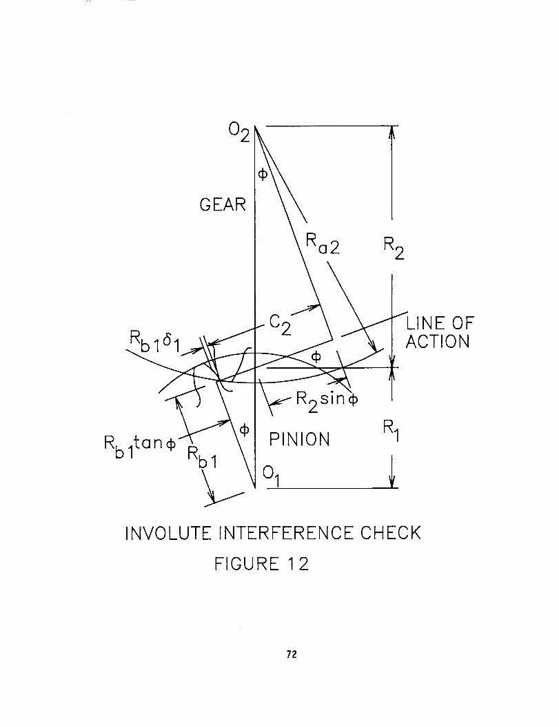
0 2
GEAR
¢,
2
C
R2
LINE OFACTION
R2sin_
PINIONRb 1
R1
INVOLUTE INTERFERENCE
FIGURE 1 2
CHECK
72
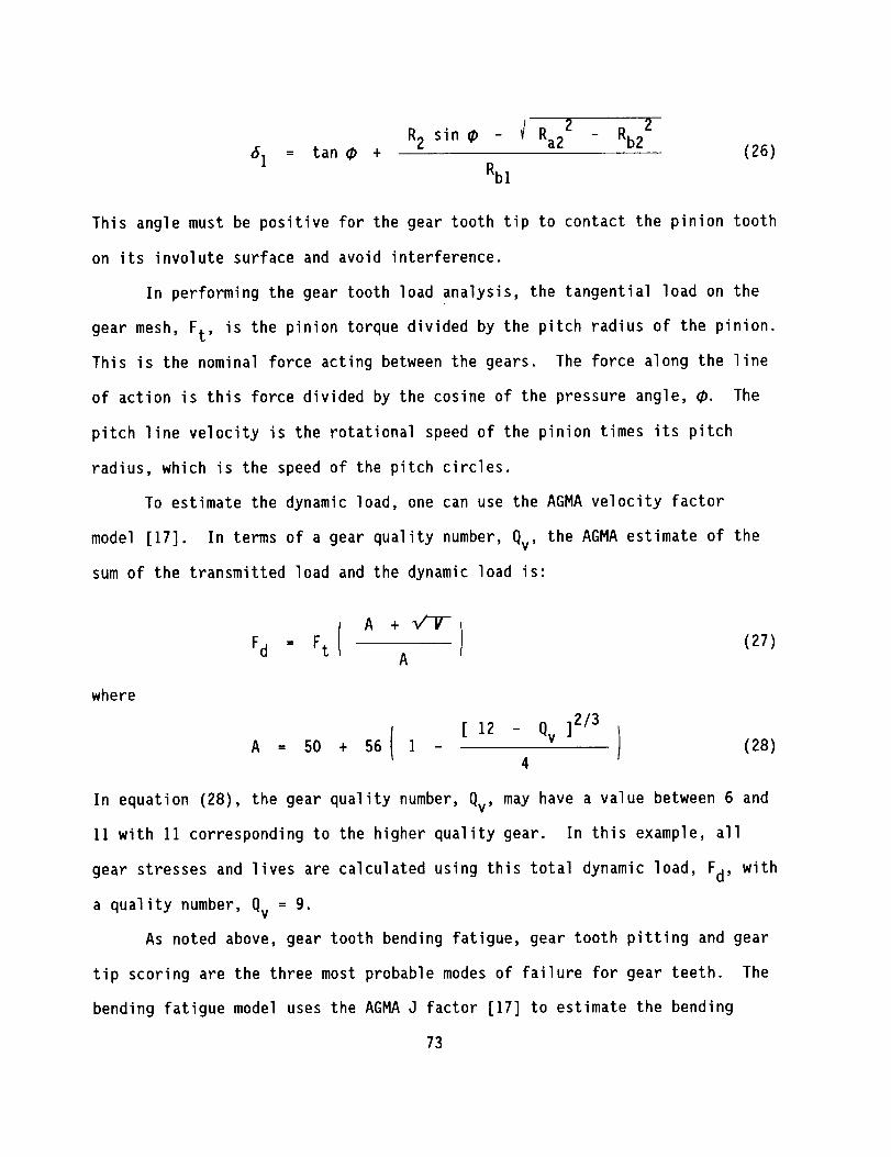
2 2R2 sin q) - I Ra2 - Rb2
61 = tan ¢ + (26)
Rb]
This angle must be positive for the gear tooth tip to contact the pinion tooth
on its involute surface and avoid interference.
In performing the gear tooth load analysis, the tangential load on the
gear mesh, Ft, is the pinion torque divided by the pitch radius of the pinion.
This is the nominal force acting between the gears. The force along the line
of action is this force divided by the cosine of the pressure angle, ¢. The
pitch line velocity is the rotational speed of the pinion times its pitch
radius, which is the speed of the pitch circles.
To estimate the dynamic load, one can use the AGMA velocity factor
model [17]. In terms of a gear quality number, Qv' the AGMA estimate of the
sum of the transmitted load and the dynamic load is:
A +_/VFd = Ft (27)A
where
[ 12 - Qv ]2/3 )A = 50 + 56 I - (28)4
In equation (28), the gear quality number, Qv' may have a value between 6 and
]I with 11 corresponding to the higher quality gear. In this example, all
gear stresses and lives are calculated using this total dynamic load, Fd, with
a quality number, Qv = g"
As noted above, gear tooth bending fatigue, gear tooth pitting and gear
tip scoring are the three most probable modes of failure for gear teeth. The
bending fatigue model uses the AGMA J factor [17] to estimate the bending
73
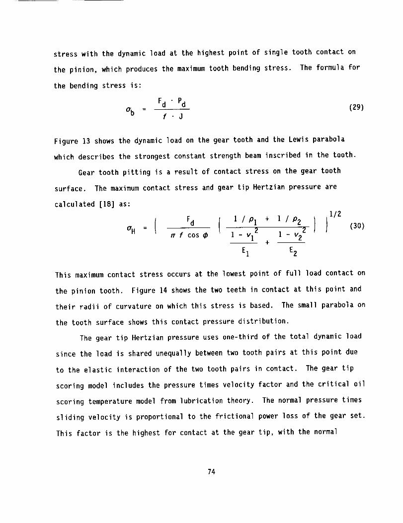
stress with the dynamic load at the highest point of single tooth contact on
the pinion, which produces the maximumtooth bending stress.
the bending stress is:
%
The formula for
_ Fd Pd (29)
f J
Figure 13 shows the dynamic load on the gear tooth and the Lewis parabola
which describes the strongest constant strength beam inscribed in the tooth.
Gear tooth pitting is a result of contact stress on the gear tooth
surface. The maximum contact stress and gear tip Hertzian pressure are
Fd I ] /Pl + 1/P2 I IOH -- I 2 2 II
rr f cos ¢ ] - vI ] - v2+
EI E2
calculated []8] as:
]/2
(30)
This maximum contact stress occurs at the lowest point of full load contact on
the pinion tooth. Figure 14 shows the two teeth in contact at this point and
their radii of curvature on which this stress is based. The small parabola on
the tooth surface shows this contact pressure distribution.
The gear tip Hertzian pressure uses one-third of the total dynamic load
since the load is shared unequally between two tooth pairs at this point due
to the elastic interaction of the two tooth pairs in contact. The gear tip
scoring model includes the pressure times velocity factor and the critical oil
scoring temperature model from lubrication theory. The normal pressure times
sliding velocity is proportional to the frictional power loss of the gear set.
This factor is the highest for contact at the gear tip, with the normal
74

TOOTHLINE OF ACTION
d / cos
FdBASE CIRCLE
LEWIS PARABOLA
MAXIMUM STRESS
GEAR TOOTH BENDING STRENGTH MODEL
FIGURE 13
75
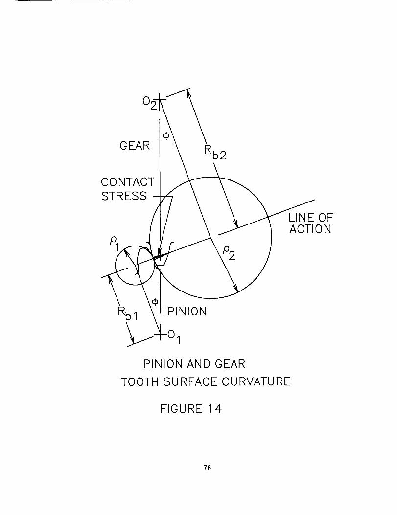
GEAR Rb2
CONTACTSTRESS
LINE OFACTION
Rb I PINION
PINION AND GEAR
TOOTH SURFACE CURVATURE
FIGURE 14-
76

pressure equal to the gear tip Hertzian pressure. The sliding velocity at the
gear tip is given by:
Vs = w 2 Ra2 sin (¢ + aa2) - w I R1 sin (¢ + al) (31)
The lubricating oil flash temperature is another factor used to monitor
gear tooth scoring. One estimate of this temperature [18] is given by:
3/4
Tf TB ( XF Fd ) I 0"45MmXMXG_/V= + I/4 i (32)
f (R] + R2)
The gear life model is based on surface pitting and is similar to the
model for rolling element bearings [19]. Its reliability estimation is based
on the two-parameter Weibull distribution:
= Ln( )kn
R 0.9 _I0
b
(33)
The life to reliability relationship of equation (33) is for a specific
load which determines the _10 life.
dynamic capacity, C, as:
This load, F, is related to the component
P
¢ ) (34)
where the dynamic capacity of the component, C, is the load which has a
90 percent reliability life of one million cycles.
For a spur gear tooth, the dynamic capacity, Ct, can be expressed as a
function of Buckingham's load-stress factor [20], B, which is a material
strength constant:
77

Ct = B ( i ) (35)
I/Pl + l/P2
With the dynamic capacity expressed in this form, the material strength
constant serves the role of the surface fatigue strength, Sac, of the AGMA
design code. A relation for the material strength constant in terms of the
surface fatigue strength is:
B __. 2 ( I - vi2 I - v22Sac EI + E2
(36)
The dynamic capacity of the whole gear is lower than that of a single
tooth due to the number of teeth subjected to the same load:
Ct
Cg - I/(b.p) (37)
Ng
The gear and pinion weights are modeled with solid discs which have
radii equal to the pitch radii of the two gears and thicknesses equal to the
face width.
Proqramminq
Table 17 summarizes this design problem in terms of the constants,
design parameters, inequality constraints and objective functions. There are
thirteen constants, three design parameters, fourteen constraints and two
objective functions in this list.
Included in the list of constants are: Poisson's ratio and the elastic
modulus for the gear material: the nominal pressure angle, ¢, and gear ratio,
n, for the mesh; the transmitted power, Hp, and pinion speed, w1; the material
weight density, y, surface constant, B, Weibull slope, b, and load-life
78

Table 17
Spur Gear Mesh Optimization Parameters
Constants
V
E
¢
n
Hp
w]
Y
B
b
P
R
TB
Pm
Design Parameters
N1
Pd
f
Inequality Constraints
61 < 0.001
f/D I < 0.5
C > 0.0
WI + W2 > 0.0
TI > 0.0
Ft > 0.0
It > 0.0
Fd > 0.0
ob < 40,000.
oH < ]50,000.
OHt < 150,000.
P Vs < 100.
Tf < 275.
tm > 2.0
Objective Function
Cmin
or
(tm)max
79

exponent, p; the desired reliability of the mesh, R; the lubricant base
temperature, TB; and the surface finish, Pm"
The three design parameters are: I) the number of teeth on the pinion,
NI; the diametral pitch, Pd; and the face width, f.
Design constraints listed are: active constraints for involute
interference and the width to diameter ratio; inactive constraints of being
positive for the center distance, weight sum, input torque, transmitted force,
pitch line velocity, and dynamic force; active bending and pitting strength
limits; active scoring limits of pressure times velocity and flash
temperature; and the mesh life bound.
The objective functions include the center distance which is to be
minimized and the mesh life which is to be maximized. In running the program,
these two functions will not be active in the same case. The listed values
are for the first objective function of minimum center distance. When the
program is run to maximize the mesh life, the center distance limit is changed
to an active limit of 2.5 inches and the mesh life constraint is changed to be
positive and thus inactive.
Subroutines BOUNDS and VALUES, developed for this example gear problem,
are listed together in Table 18. These two routines call a series of analysis
subroutines to evaluate the properties of the gear design. These subroutines:
DYNAM, MESH, GLIFE, GEARWT and TEMPER are also listed in Table ]8 along with
LEWIS which MESH calls. Subroutine DYNAM determines the dynamic load in the
mesh with the AGMA velocity factor calculation using equations (27) and (28).
Subroutine MESH performs a kinematic analysis of the gear mesh geometry and
calculates the bending stresses and Hertzian contact stresses on the teeth in
the mesh with equations (26) and (29) through (31). MESH also calculates the
80

Table 18
Spur Gear Mesh Constraint and Objective Function Evaluation Routines
C
C
C
C
C
C
CC
C
C
C
C
C
C
C
C
C
C
C
C
C
C
C
C
C
C
C
C
C
C
CC
C
C
C
C
C
C
C
C
C
CC
C
C
CC
SUBROUTINE BOUNDS(CONST,NCO,X,NX,VCSTR,NCS)
BOUNDS DETERMINES THE PRESENT CONSTRAINTFUNCTION VALUES
FOR A SPUR GEAR LIFE DESIGN EXAMPLE
PARAMETERS:
CONST - FIXED DESIGN CONSTANT
NCO - NUMBER OF DESIGN CONSTANTS
NCS - NUMBER OF INEQUALITY CONSTRAINTSNX - NUMBER OF INDEPENDENT DESIGN VARIABLES
VCSTR - PRESENT CONSTRAINT VALUES
X - PRESENT DESIGN VARIABLE VALUES
ALL VALUES ARE IN PROBLEM UNITS (UNSCALED)
CONST(1) = mu
CONST(2) = E
CONST(3) = PHI
CONST(4) = N
CONST(5) = Hp
- POISSON'S RATIO
- ELASTIC MODULUS (PSI)
- PRESSURE ANGLE (DEGREES)- GEAR RATIO
- PINION POWER (HORSEPOWER)
CONST(6) = Np - PINION SPEED (RPM)
CONST(7) = GAMMA - MATERIAL WEIGHT DENSITY (LBS/IN**3)
CONST(8) = Bc - MATERIAL STRENGTH CONSTANT (PSI)
CONST(9) = b
CONST(IO)= p
CONST(ll)= Rel
CONST(12)= TbCONST(13)= RMS
- WEIBULL SLOPE
- LOAD-LIFE FACTOR
- DESIGN RELIABILITY
- OIL INLET TEMPERATURE (DEGREES F)
- TOOTH SURFACE FINISH (RMS)
VCSTR(1) = DELl - INVOLUTE INTERFERENCE ANGLE (RADIANS)
VCSTR(2) = LAMMIN - FACE WIDTH TO PINION DIAMETER RATIO
VCSTR(3) = C
VCSTR(4) = WT
VCSTR(5) = Tq
VCSTR(6) = Ft
VCSTR(7) = V
VCSTR(8) = Fd
VCSTR(9) = BDSTR
VCSTR(IO)= HZSTRVCSTR(11)= TIPPR
VCSTR(12)= PVF
VCSTR(13)= Tf
VCSTR(14)= Lm
- CENTER DISTANCE (INCHES)- PINION & GEAR WEIGHTS (POUNDS)
- PINION TORQUE (POUND - INCHES)
- TRANSMITTED FORCE (POUNDS)
- PITCH LINE VELOCITY (FT/MIN)
- DYNAMIC LOAD (POUNDS)- AGMA BENDING STRESS (PSI)
- CONTACT PRESSURE (PSI)
- GEAR TIP HERTZ CONTACT PRESSURE (PSI)- PRESSURE TIMES VELOCITY FACTOR
(10"'6 PSI-FT/MIN)
- FLASH TEMPERATURE (DEGREES F)
- MESH LIFE (10"'3 HOURS)
81

CCCCC
Table 18 Continued
Spur Gear Mesh Constraint and Objective Function Evaluation Routines
X(l) : nl
X(2) : Pd
X(3) : Wd
- NUMBER OF PINION TEETH
- DIAMETRAL PITCH (1.O/IN)
- FACE WIDTH (INCHES)
DIMENSION X(NX),VCSTR(NCS),CONST(NCO)REAL LM,LP,LGPI : 3.14159265
POI = CONST(I)
E = CONST(2)
PHI = CONST(3)RATIO = CONST(4)
HP = CONST(5)
RPM = CONST(6)GAM = CONST(7)
BC = CONST(8)
B = CONST(9)
P = CONST(]O)
REL = CONST(]I)
TB = CONST(12)
RMS = CONST(]3)
TNI = X(1)
PD = X(2)
WD : X(3)TN2 = RATIO*TNIPHIR : PHI*PI/180.ORP : O.5*TNI/PDRG : RATIO*RPC : RP*( 1.0 + RATIO )V = RPM*RP*PI/6.0TQ : HP*63025.0/RPMFT = TQ/RPCALL DYNAM(FT,V,DL)TDQ : RP*DLCALL MESH(PHI,PD,TNI,TN2,E,POI,WD,TDQ,RPM,CMP,DELI,RHI,
1 PVF,TIPHZ,TIPBS,HZSTR,BDSTR)RH2 = C*SlN(PHIR) - RHICALL GLIFE(DL,WD,RHI,RH2,TNI,TN2,RPM,BC,B,P,REL,
I LM,LP,LG,CYLP,CYLG)CALL GEARWT(GAM,GAM,RP,RG,WD,PW,GW)CALL TEMPER(PD,PHI,TNI,TN2,WD,DL,V,TB,RMS,TF,CSN)VCSTR(1) : DELlVCSTR(2) = WD/(2.0*RP)VCSTR(3) = CVCSTR(4) = PW + GWVCSTR(5) : TQVCSTR(6) : FTVCSTR(7) = V
82
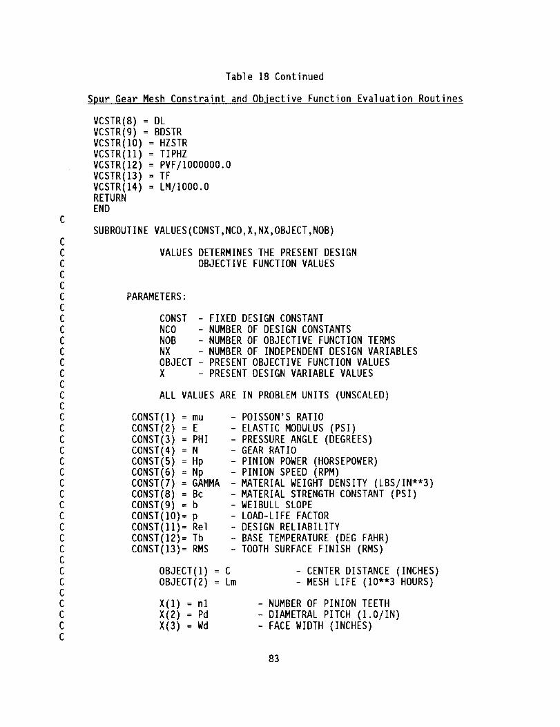
CCCCCCCCCCCCCCCCCCCCCCCCCCCCCCCCCCCCC
Table 18 Continued
Spur Gear Mesh Constraint and Objective Function Evaluation Routines
VCSTR(8) : DL
VCSTR(9) : BDSTR
VCSTR(IO) : HZSTR
VCSTR(II) = TIPHZ
VCSTR(12) = PVF/IO00000.O
VCSTR(13) = TF
VCSTR(14) = LM/IO00.ORETURN
END
SUBROUTINE VALUES(CONST,NCO,X,NX,OBJECT,NOB)
VALUES DETERMINES THE PRESENT DESIGN
OBJECTIVE FUNCTION VALUES
PARAMETERS:
CONST - FIXED DESIGN CONSTANT
NCO - NUMBER OF DESIGN CONSTANTS
NOB - NUMBER OF OBJECTIVE FUNCTION TERMS
NX - NUMBER OF INDEPENDENT DESIGN VARIABLES
OBJECT - PRESENT OBJECTIVE FUNCTION VALUES
X - PRESENT DESIGN VARIABLE VALUES
ALL VALUES ARE IN PROBLEM UNITS (UNSCALED)
CONST(1) : mu
CONST(2) = E
CONST(3) = PHI
CONST(4) = NCONST(5) = Hp
CONST(6) = Np
CONST(7) = GAMMA
CONST(8) = Bc
CONST(9) = b
CONST(IO)= p
CONST(II)= Rel
CONST(12)= Tb
CONST(13)= RMS
- POISSON'S RATIO
- ELASTIC MODULUS (PSI)
- PRESSURE ANGLE (DEGREES)- GEAR RATIO
- PINION POWER (HORSEPOWER)
- PINION SPEED (RPM)
- MATERIAL WEIGHT DENSITY (LBS/IN**3)
- MATERIAL STRENGTH CONSTANT (PSI)- WEIBULL SLOPE
- LOAD-LIFE FACTOR
- DESIGN RELIABILITY
- BASE TEMPERATURE (DEG FAHR)
- TOOTH SURFACE FINISH (RMS)
OBJECT(1) : C
OBJECT(2) = Lm
- CENTER DISTANCE (INCHES)
- MESH LIFE (10"'3 HOURS)
X(I) : nl
X(2) : Pd
X(3) = Wd
- NUMBER OF PINION TEETH
- DIAMETRAL PITCH (I.O/IN)
- FACE WIDTH (INCHES)
83
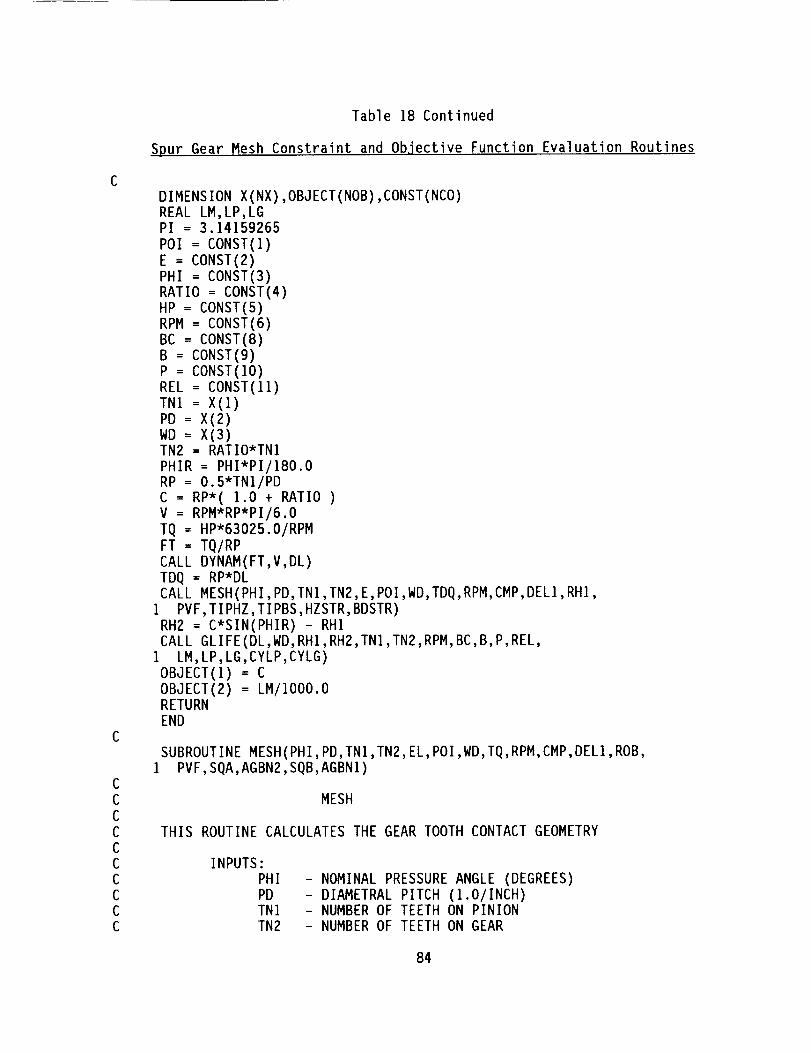
Table 18 Continued
Spur Gear Mesh Constraint and Objective Function Evaluation Routines
DIMENSION X(NX),OBJECT(NOB),CONST(NCO)REAL LM,LP,LGPI = 3.14159265
POI = CONST(I)
E = CONST(2)
PHI : CONST(3)RATIO = CONST(4)
HP = CONST(5)
RPM = CONST(6)
BC = CONST(8)
B = CONST(9)
P = CONST(IO)
REL = CONST(11)
TNI = X(1)
PD = X(2)
WD : X(3)TN2 = RATIO*TNIPHIR = PHI*PI/180.ORP = O.5*TNI/PDC : RP*( 1.0 + RATIO )V = RPM*RP*PI/6.0TQ : HP*63025.0/RPMFT : TQ/RPCALL DYNAM(FT,V,DL)TDQ : RP*DLCALL MESH(PHI,PD,TNI,TN2,E,POI,WD,TDQ,RPM,CMP,DELI,RHI,
I PVF,TIPHZ,TIPBS,HZSTR,BDSTR)RH2 = C*SlN(PHIR) - RHICALL GLIFE(DL,WD,RHI,RH2,TNI,TN2,RPM,BC,B,P,REL,
I LM,LP,LG,CYLP,CYLG)OBJECT(1) = COBJECT(2) : LM/IO00.ORETURNEND
SUBROUTINE MESH(PHI,PD,TNI,TN2,EL,POI,WD,TQ,RPM,CMP,DELI,ROB,
I PVF,SQA,AGBN2,SQB,AGBNI)
MESH
THIS ROUTINE CALCULATES THE GEAR TOOTH CONTACT GEOMETRY
INPUTS:PHIPDTNITN2
- NOMINAL PRESSURE ANGLE (DEGREES)
- DIAMETRAL PITCH (I.0/INCH)- NUMBER OF TEETH ON PINION
- NUMBER OF TEETH ON GEAR
84

Table 18 Continued
Spur Gear Mesh Constraint and Objective Function Evaluation Routines
C
C
C
EL
POI
WD
TQRPM
- ELASTIC MODULUS OF TEETH (PSI)
- POISSON'S RATIO FOR TEETH
- TOOTH FACE WIDTH (INCHES)
- TORQUE APPLIED TO PINION (POUND - INCHES)- SPEED OF PINION IN REVOLUTIONS PER MINUTE
OUTPUTS:
CMP
DELl
- MESH CONTACT RATIO- DISTANCE FROM PINION BASE CIRCLE TANGENCY
TO TIP OF GEAR TOOTH ALONG LINE OF ACTION
MEASURED AS A PINION ROLL ANGLE
ROB - PINION TOOTH SURFACE RADIUS OF CURVATURE
AT THE LOWEST POINT OF SINGLE TOOTH CONTACT C
PVF - SCORING FACTOR (PSI-FT/MIN / 10"'6)
SQA - HERTZIAN CONTACT STRESS AT TIP OF GEAR TOOTH
(PSl)AGBN2 - AGMA BENDING STRESS FOR HALF LOAD AT TIP
OF GEAR TOOTH (PSI)
SQB - HERTZIAN CONTACT STRESS AT LOWEST POINT OF
SINGLE TOOTH CONTACT (PSI)AGBNI - AGMA BENDING STRESS FOR FULL LOAD AT
HIGHEST POINT OF SINGLE TOOTH CONTACT (PSI) C
ACS(A)=ATAN(SQRT(I.-A*A)/A)ASN(A)=ATAN(A/SQRT(I.-A*A))
FINV(A)=SIN(A)/COS(A)-ANW=OPI=3.14159265
IT IS ASSUMED THAT THE PINION IS THE DRIVING GEAR
J=1FJ=J
ADD=I.
DED=1.25
RFR=O.3
IF(PD.GE.20.O) DED=I. 2+O.O02*PDADDI=ADD
ADD2 =ADD
DDDI=DED
ADI=ADDI/PD
AD2=ADD2/PD
DDI=DDDI/PD
RF=RFR/PD
PC=PI/PD
RAD--180./PI
P=PHI/RAD
COP=COS(P)
SIP=SIN(P)
85

Table 18 Continued
Spur Gear Mesh Constraint and Objective Function Evaluation Routines
C
C
C
C
C
C
CCCCCC
PB=PC*COP
RI=O.5*PC*TNI/PI
R2=O.5*PC*TN2/PIRBI=RI*COP
RB2=R2*COP
RAI=RI+ADIRA2=R2+AD2*FJ
C=FJ*RI+R2
CI=SQRT(RAI*RAI-RBI*RBI)
C2=SQRT(RA2*RA2-RB2*RB2)
Z=CI+(C2-C*SIP)*FJ
CMP=Z/PBAAI=(C2-R2*SIP)/RBI*FJ
AA2=(C2-R2*SIP)/RB2*FJ
DELI=SIP/COP-AAI
IF DELl LESS THAN O INTERFERENCE WILL HAPPEN
SET EQUAL TO A SMALL VALUE TO GENERATELARGE CONTACT STRESSES
IF(DELI.LT.O.O) DELl = O.00I*SIP/COP
AB2=(CI-RI*SIP)/RB2
DEL2=SIP/COP-AB2IF(J.LT.O) DEL2=SIP/COP-AA2
IF DEL2 LESS THAN 0 INTERFERENCE WILL HAPPEN
SET EQUAL TO A SMALL VALUE TO GENERATELARGE CONTACT STRESSES
IF(DEL2.LT.O.O) DEL2 = O.00I*SIP/COP
BLI:(Z-PB)/RBI
BHI=(2.*PB-Z)/RBITLI=DELI+BLITUI=TLI+BHI
RAT=TN2/TNI
IF(J.GT.O) GO TO 5
TP=FINV(P)
PAI=ACS(RBI/RAI)PA2=ACS(RB2/RA2)
TAI=FINV(PAI)
TA2=FINV(PA2)
BETAI=ACS((RA2*RA2-RAI*RAI-C*C)/(2.0*C*RAI))
BETA2=ASN(RAI*SIN(BETAI)/RA2)GAMMAI=BETAI+TAI-TP
GLIM2=BETA2+TA2-TP
GAMMA2=TNI*GAMMAI/TN2
86

Table 18 Continued
Spur Gear Mesh Constraint and Objective Function Evaluation Routines
IF(GAMMA2.GT.GLIM2) GO TO 5
XINT=RA2*(GLIM2-GAMMA2)
WRITE (NW,122) XINT
122 FORMAT(//' SECONDARY INVOLUTE INTERFERENCE'/I ' TOOTH TIP OVERLAP = ',F8.5,' INCHES AT ENTRY'/
2 ' INCREASE N2/NI TO AVOID THIS INTERFERENCE'/)5 CONTINUE
FSIN = TQ/RI
FTIP = FSIN/3.0
EO=EL/(I.-POI*POI)ROA=RBI*DELIROB=RBI*TLI
CAPI=I./(ROA*(I.-FJ*ROA/(C*SIP)))
CAP2=I./(ROB*(I.-FJ*ROB/(C*SIP)))
SBA=SQRT(2.*FTIP/(COP*PI*EO*WD*CAPI))
SQA=FTIP/(COP*PI*WD*SBA)
SBB=SQRT(2.*FSIN/(COP*PI*EO*WD*CAP2))
SQB=FSIN/(COP*PI*WD*SBB)
PUI=ATAN(TUI)*RAD
TC=PC/2.CALL LEWIS(PHI,DDI,TC,RF,PD,TNI,PUI,YS,AKS)
SBNDI=FSIN*PD/(WD*YS)AGBNI=SBND]*AKS
TTI=TUI+BLI
PTI=ATAN(TTI)*RAD
CALL LEWIS(PHI,DDI,TC,RF,PD,TNI,PTI,YT,AKT)
SBND2=FTIP*PD/(WD*YT)AGBN2=SBND2*AKT
RTPI=RA2*SIN(AA2)/SIN(AAI)OMEGA=RPM*2.*PI
VLG=(OMEGA/RAT)*RA2*SIN(P+AA2)VLP=OMEGA*RTPI*SIN(P-AAI)
PVF=SQA*(VLG-VLP)/I2.RETURN
END
SUBROUTINE LEWIS(PHI,B,TC,RF,PD,TN,PHIA,Y,AK)
LEWIS CALCULATES THE LEWIS FORM FACTOR FOR A PINION TOOTH
PHI = THE PITCH LINE PRESSURE ANGLE IN DEGREES
B = THE PINION DEDENDUM IN INCHES
TC = THE PITCH CIRCLE TOOTH THICKNESS IN INCHES
RF = THE CUTTER TIP RADIUS IN INCHES
PD = THE DIAMETRAL PITCH IN I./INCHESTN = THE PINION TOOTH NUMBER
PHIA = THE PRESSURE ANGLE AT THE POINT OF CONTACT
FOR WHICH Y IS CALCULATED IN DEGREES
87
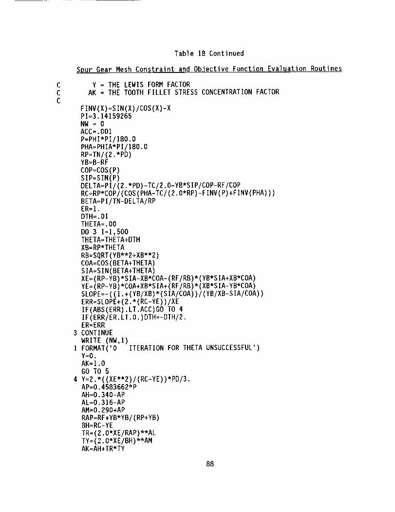
Table 18 Continued
Spur Gear Mesh Constraint and Objective Function Evaluation
Y = THE LEWIS FORM FACTOR
AK = THE TOOTH FILLET STRESS CONCENTRATION FACTOR
FINV(X)=SIN(X)/COS(X)-XPI=3.I4159265
NW = 0
ACC=.O01
P=PHI*PI/180.O
PHA=PHIA*PI/180.O
RP=TN/(2.*PD)YB=B-RF
COP=COS(P)
SIP=SIN(P)
DELTA=PI/(2.*PD)-TC/2.0-YB*SIP/COP-RF/COP
RC=RP*COP/(COS(PHA-TC/(2.0*RP)-FINV(P)+FINV(PHA)))
BETA=PI/TN-DELTA/RPER=I.DTH=.01
THETA=.O0
DO 3 I=1,500THETA=THETA+DTH
XB=RP*THETA
RB=SQRT(YB**2+XB**2)
COA=COS(BETA+THETA)
SIA=SIN(BETA+THETA)
XE=(RP-YB)*SIA-XB*COA-(RF/RB)*(YB*SIA+XB*COA)
YE=(RP-YB)*COA+XB*SIA+(RF/RB)*(XB*SIA-YB*COA)SLOPE=-((I.+(YB/XB)*(SIA/COA))/(YB/XB-SIA/COA))
ERR=SLOPE+ (2.*(RC-YE))/XE
IF(ABS(ERR).LT.ACC)GO TO 4
IF(ERR/ER. LT. O. )DTH=-DTH/2.ER=ERR
CONTINUE
WRITE (NW, 1)FORMAT('O ITERATION FOR THETA UNSUCCESSFUL')Y=O.
AK=1.0
GO TO 5
Y=2. *((XE**2) /(RC-YE))*PD/3.AP=O.4583662*P
AH=O.340-AP
AL=O.316-AP
AM=O. 290+AP
RAP=RF+YB*YB/(RP+YB)BH=RC-YE
TR= (2.O*X E/RAP) **AL
TY= (2.O*X E/BH )**AMAK=AH+TR*TY
Routines
88

Table 18 Continued
Spur Gear Mesh Constraint and Objective Function Evaluation Routines
C
C
C
C
C
C
C
C
C
C
C
C
C
C
C
C
C
C
C
C
C
C
C
C
C
C
C
5 RETURN
END
SUBROUTINE GLIFE(FORCE,WD,RHP,RHG,TNP,TNG,PINRPM,BC,B,P,REL,
I LM,LP,LG,CYLP,CYLG)
SUBROUTINE TO CALCULATE THE LIFE OF A GEAR MESH
INPUTS
FORCE
WD
RHP
RHG
TNP
TNG
PINRPM
BC
B
P
REL
= NORMAL TOOTH LOAD IN POUNDS
= EFFECTIVE FACE WIDTH IN INCHES
= PINION CONTACT RADIUS OF CURVATURE IN INCHES
= GEAR CONTACT RADIUS OF CURVATURE IN INCHES
= NUMBER OF TEETH ON PINION AS A REAL VARIABLE
= NUMBER OF TEETH ON GEAR AS A REAL VARIABLE
= PINION SPEED IN REVOLUTIONS PER MINUTE
= MATERIAL STRENGTH CONSTANT IN PSI
= WEIBULL SLOPE
= LOAD LIFE FACTOR
= DESIRED RELIABILITY AS A DECIMAL
OUTPUTS
LM
LP
LG
CYLP
CYLG
= MESH LIFE IN HOURS
= PINION LIFE IN HOURS
= GEAR LIFE IN HOURS
= PINION LIFE IN MILLION ROTATIONS
= GEAR LIFE IN MILLION ROTATIONS
REAL LM,LP,LGCT = BC*WD/(I.O/RHP + I.O/RHG)
EX = I.O/(B*P)
CP = CT*(I.0/TNP)**EX
CG = CT*(I.O/TNG)**EX
PLIO = (CP/FORCE)**P
GLIO = (CG/FORCE)**P
BR = I.O/B
RATLF = (ALOG(REL)/ALOG(O.g))**BRCYLP = PLIO*RATLF
CYLG = GLIO*RATLF
LP = CYLP*IOOOOOO.O/(60.O*PINRPM)
LG = CYLG*IOOOOOO.O*TNG/(60.O*PINRPM*TNP)
LM = 1.0/((I.O/TP)**B + (I.0/TG)**B)**BRRETURN
END
89

Table 18 Continued
C
C
C
CC
C
C
C
C
C
C
C
C
C
CC
C
C
C
C
C
C
C
CC
C
C
C
C
C
C
C
Spur Gear Mesh Constraint and Objective Function Evaluation Routines
SUBROUTINE DYNAM (FT,V,DL)
DYLOAD CALCULATES THE DYNAMIC LOAD OF THE MESHING OF
THE GEARS USING THE AGMA VELOCITY FACTOR
DL = THE DYNAMIC LOAD DUE TO THE MESHING
INPUTS:
FT
V= THE TRANSMITTED LOAD (POUNDS)
= THE PITCH LINE VELOCITY (FT/MIN)
OUTPUT:
DL = THE TOTAL DYNAMIC LOAD (POUNDS)
QV = 9.0
A = 50.0 + 56.0"(1.0 - (12.0 - QV)**(2.0/3.0))/4.0
VF = ( A + SQRT(V) )/ADL = FT*VF
RETURN
END
SUBROUTINE TEMPER(PD,PHI,TNI,TN2,WD,DL,V,TB,RMS,TF,CSN)
TEMPER IS A SUBROUTINE THAT CALCULATES THE FLASH
TEMPERATURE, THE CRITICAL SCORING NUMBER AND THE MINIMUMELASTOHYDRODYNAMIC FILM THICKNESS FOR TWO GEARS IN MESH
PHI
TNI,TN2PD
V
RMS
RA2
RB2
WD
DL
TB
C2
TF
FT
= PRESSURE ANGLE IN DEGREES
= NUMBER OF TEETH ON PINION AND GEAR
= DIAMETRAL PITCH
= PITCH LINE VELOCITY (FEET/MINUTE)
= TOOTH SURFACE FINISH (RMS)= GEAR ADDENDUM RADIUS
= GEAR BASE RADIUS
= FACE WIDTH
= TOOTH DYNAMIC LOAD (POUNDS)= INLET OIL TEMPERATURE
= RADIUS OF CURVATURE AT TIP OF GEAR TOOTH
= FLASH TEMPERATURE
= NORMAL TOOTH LOAD IN POUNDS
PI = 3.14159265
P = PHI*PI/I80.O
COP = COS(P)
SIP = SIN(P)
RI = TN]/(2.0*PD)R2 = TN2/(2.0*PD)C = R] + R2
90

C
CCCCCCCCC
Table I8 Continued
Spur Gear Mesh Constraint and Objective Function Evaluation Routines
GR = TN2/TNI
RPM = 6.0*V/(PI*RI*COP)
RAT = RI + 1.0/PDRBI = RI*COP
CI = SQRT(RAI*RAI - RBI*RBI)
TAT = CI/RBI
TAP = SIP/COP
GY = TAT/TAP - 1.0
FD IS THE NORMAL FORCE ON THE GEAR
FD = DL/3.0
CRITICAL SCORING TEMPERATURE OF THE GEAR
XM = 1.75
AX = ABS(SQRT(I.O + GY) - SQRT(I.O - GY/GR))
BX = ((1.0 + GY)*(GR - GY))**0.25
XG = 0.5I*SQRT(GR + 1.0)*AX/BX
SW = (FD/WD)**(0.75)
TI = SW*(0.027"50.0/(50.0 - RMS))*XM*XG*SQRT(V)/(C**O.25)TF = TB + TI
CRITICAL SCORING NUMBER
CSN = SW*SQRT(RPM)/(PD**.25)RETURN
END
SUBROUTINE GEARWT (RHOI,RHO2,RI,R2,WD,PW,GW)
GEARWT CALCULATES THE WEIGHT OF THE PINION AND GEAR
IN MESH
RHOI,RH02
RI,R2WD
PW
GW
= MATERIAL DENSITY OF THE RESPECTIVE GEARS
= PITCH RADIUS OF THE PINION AND GEAR
= FACE WIDTH OF GEARS
= PINION WEIGHT
= GEAR WEIGHT
PI = 3.14159265PW = RHOI*PI*RI**2 *WD
GW = RHO2*PI*R2**2 *WD
RETURN
END
91

pressure times velocity at the gear tip to model potential scoring. In order
to calculate the bending stresses, subroutine MESHcalls subroutine LEWIS
which performs an interval halving iteration to determine the size of the
largest inscribed parabola in the tooth. Subroutine GLIFE performs a Weibull
analysis with equations (33) through (37) to estimate the life of the gear
mesh for the reliability specified in the constant list. Subroutine GEARWT
estimates the weights of the pinion and the gear and subroutine TEMPER
calculates the flash temperature for the meshusing equation (32) to determine
the potential for scoring damage.
Any permissible subroutine namesmay be used in programming for a
specific problem as long as the namesof the subroutines in SEEKare avoided.
These namesare listed in the file SEEK.DOC,which is Appendix A, and in
Table I of the programming section and are: BACK,BOUNCE,BOUNDS,CHECK,
GRADNT,MERIT, RESIZE,SCAN,SCOUT,SIZE, UNIT, VALUESand WALL. Once the
problem subroutines have been written, they need to be compiled and linked to
the compiled program SEEK.OBJto produce an executable program with a name
such as GEAR.EXE. With this program, various optimal gear designs can be
found using different input files.
Numerical Example
For an example, let us consider the design of a gear set to transmit
10 horsepower from a shaft turning at 4,500 RPM to an output shaft turning at
3,000 RPM. The center distance of the gears should be minimized for a mesh
life of at least 2,000 hours with a reliability of 90 percent. The face width
ratio is to be less than or equal to 0.5, the material strengths are
40,000 psi in bending and 150,000 psi surface endurance, the PV factor limit
92

is ]00 million psi-ft/min and the flash temperature limit is 275 degrees
Fahrenheit.
Table 19 is a listing of the input file defining this example. Rules
for writing the input data file are given in "SEEK.DOC,"which is listed in
Appendix A. The data file starts with the problem title. On the next line is
the numberthirteen, and the following thirty-nine lines contain the problem
constants as listed in Table 17, their definitions and their units. The
material surface constant of 9,800 psi corresponds to a surface compression
endurance strength of 200,000 psi at 107 fatigue cycles and a reliability of
90 percent. The load-life factor of 8.93 is from the ANSI/AGMA2001 B88
Standard, and the Weibull slope of 2.5 is from the NASALewis gear test data
[21]. Following the constants is a line with the numberthree for the number
of independent design parameters, which are on the next nine lines with their
ranges, initial values, definitions and units. The number fourteen follows on
the next line, with the fourteen constraint limits, their directions and their
namesand units on the following forty-two lines. After these comesa line
with the optimization direction, MIN, and a line with the numbertwo for the
numberof objective function terms. The first term is the center distance
which has a weighting coefficient of one and the units of inches, and the
second is the meshlife with a weighting coefficient of zero and units of
thousand hours.
Running the program GEAR.EXEwith this data file produced the output
data file listed in Table 20. The first page lists the problem constants,
design parameters and constraint limits as provided by the input data file but
in a little more readable form. The second page lists the merit function
terms and notes that an optimumwas found in thirty-three steps. It then
93
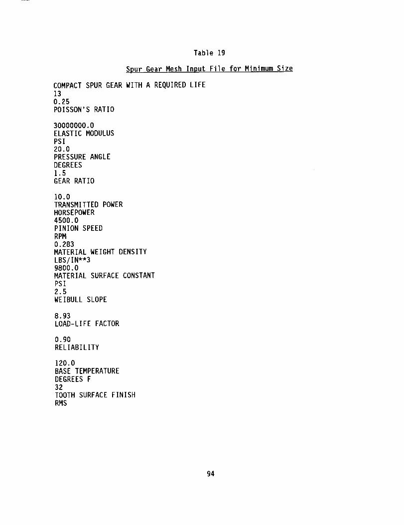
Table 19
Spur Gear Mesh Input File for Minimum Size
COMPACT SPUR GEAR WITH A REQUIRED LIFE
13
0.25
POISSON'S RATIO
30000000.0
ELASTIC MODULUS
PSI
20.0
PRESSURE ANGLE
DEGREES
1.5
GEAR RATIO
10.0TRANSMITTED POWER
HORSEPOWER
4500.0
PINION SPEED
RPM
O.283
MATERIAL WEIGHT DENSITY
LBS/IN**39800.0
MATERIAL SURFACE CONSTANT
PSI
2.5
WEIBULL SLOPE
8.93
LOAD-LIFE FACTOR
0.90
RELIABILITY
120.0
BASE TEMPERATURE
DEGREES F
32TOOTH SURFACE FINISH
RMS
94

Table 19 Continued
3
10.0 100.0 40.0
PINION TEETH
Spur Gear Mesh Input File for Minimum Size
4.0 28.0 10.0
DIAMETRAL PITCH
I.O/INCHES0.5 5.0 2.5
FACE WIDTH
INCHES
14
LOWER 0.001
INVOL. INTERFERENCE
RADIANS
UPPER O. 5
FACE WIDTH TO DIAMETER
RAT I0
LOWER O.0
CENTER DISTANCEINCHES
LOWER O.0
GEAR AND PINION WEIGHT
POUNDS
LOWER O.0
PINION TORQUELB-IN
LOWER O.0
TRANSMITTED FORCE
POUNDS
LOWER O. 0
PITCH LINE VELOCITY
FT/MINLOWER O. 0
TOTAL DYNAMIC LOAD
POUNDS
UPPER 40000.0
AGMA BENDING STRESSPSI
UPPER 150000.0
FULL LOAD CONTACT STRESS
PSI
UPPER 150000.0
GEAR TIP HERTZ PRESSURE
PSI
UPPER 100.0PV FACTOR
M PSI-FT/MIN
95

UPPER 275.0
FLASH TEMPERATURE
DEGREES F
LOWER 2.0
MESH LIFE
10"'3 HOURS
MIN
2
1.0
CENTER DISTANCE
INCHES
0.0
MESH LIFE
10"'3 HOURS
Table 19 Continued
Spur Gear Mesh Input File for Minimum Size
96

Table 20
Spur Gear Mesh Output File for Minimum Size
COMPACT SPUR GEAR WITH A REQUIRED LIFE
DESIGN WITH MODIFIED GRADIENT OPTIMIZATION
USING A MAXIMUM STEP LIMIT AND SCALED VARIABLES.
FIXED DESIGN REQUIREMENTS:
I POISSON'S RATIO
2 ELASTIC MODULUS
3 PRESSURE ANGLE
4 GEAR RATIO
5 TRANSMITTED POWER
6 PINION SPEED7 MATERIAL WEIGHT DENSITY
8 MATERIAL SURFACE CONSTANT
9 WEIBULL SLOPE
IO LOAD-LIFE FACTOR
11 RELIABILITY
12 BASE TEMPERATURE13 TOOTH SURFACE FINISH
0.25000
30000000.00000 PSI
20.00000 DEGREES
1.50000
10.00000 HORSEPOWER
4500.00000 RPM
0.28300 LBS/IN**39800.00000 PSI
2.50000
8.93000
0.90000
120.00000 DEGREES F
32.00000 RMS
THERE ARE 3 INDEPENDENT DESIGN VARIABLES.
ESTIMATED VALUES:
LOW HIGH INITIAL
I PINION TEETH
2 DIAMETRAL PITCH
3 FACE WIDTH
10.00000 100.00000 40.00000
4.00000 28.00000 I0.00000 1.0/INCHES0.50000 5.00000 2.50000 INCHES
THE 14 CONSTRAINT LIMITS ARE:
I INVOL. INTERFERENCE
2 FACE WIDTH TO DIAMETER
3 CENTER DISTANCE4 GEAR AND PINION WEIGHT
5 PINION TORQUE6 TRANSMITTED FORCE
7 PITCH LINE VELOCITY
8 TOTAL DYNAMIC LOAD
9 AGMA BENDING STRESSIO FULL LOAD CONTACT STRESS
11 GEAR TIP HERTZ PRESSURE
12 PV FACTOR
13 FLASH TEMPERATURE14 MESH LIFE
40000
150000
150000
I00
275
2
O.OOlO0
0.50000
0.00000
0.00000
0.00000
0.00000
0.00000
0 00000
00000
00000
00000
00000
0000000000
TYPE
RADIANS LOWER
RATIO UPPERINCHES LOWER
POUNDS LOWER
LB-IN LOWER
POUNDS LOWER
FT/MIN LOWERPOUNDS LOWER
PSI UPPER
PSI UPPER
PSI UPPER
M PSI-FT/MIN UPPERDEGREES F UPPER
10"'3 HOURS LOWER
97

Table 20 Continued
Spur Gear Mesh Output File for Minimum Size
MINIMIZE THE OBJECTIVE FUNCTION, WHICH HAS 2 TERMS.
OBJ = THE LINEAR SUM OF:
! CENTER DISTANCE IN INCHES TIMES
2 MESH LIFE IN 10"'3 HOURS TIMES
1.0000
0.0000
OPTIMIZATION SUCCESSFUL IN
THE FINAL DESIGN VECTOR IS:
33 STEPS
X(1)
] PINION TEETH 20.39544
2 DIAMETRAL PITCH 13.91159 ].O/INCHES3 FACE WIDTH 0.73295 INCHES
THE MINIMUM OBJECTIVE FUNCTION =
I CENTER DISTANCE
2 MESH LIFE
].83259 , ITS COMPONENTS ARE:
= 1.8326 INCHES TIMES
= 2.0065 ]0**3 HOURS TIMESl.O0000.0000
THE LAST CHANGE IN THE OBJECTIVE FUNCTION = -0.326633E-04
THE LAST STEP CHANGE SIZE FOR THE DESIGN VARIABLE = 0.976563E-04
THE 14 CONSTRAINT VALUES ARE:
I INVOL. INTERFERENCE
2 FACE WIDTH TO DIAMETER
3 CENTER DISTANCE
4 GEAR AND PINION WEIGHT
5 PINION TORQUE6 TRANSMITTED FORCE
7 PITCH LINE VELOCITY
8 TOTAL DYNAMIC LOAD
9 AGMA BENDING STRESS
10 FULL LOAD CONTACT STRESS
11 GEAR TIP HERTZ PRESSURE
12 PV FACTOR
13 FLASH TEMPERATURE
14 MESH LIFE
LIMIT
= .10861 RADIANS .I0000E-02= .49980 RATIO .50000
= 1.8326 INCHES .00000
= 1.1376 POUNDS .00000
= 140.06 LB-IN .00000
= 191.07 POUNDS .00000
= 1727.1 FT/MIN .00000= 4]8.72 POUNDS .00000
= 25097. PSI 40000.= .14999E+06 PSI .15000E+06
= .]2518E+06 PSI .15000E+06
= 92.633 M PSI-FT/MIN IO0.O0= 216.49 DEGREES F 275.00
= 2.0006 10"'3 HOURS 2.0000
TYPE
LOWER
UPPER
LOWER
LOWER
LOWERLOWER
LOWER
LOWER
UPPER
UPPER
UPPER
UPPER
UPPER
LOWER
98

Table 20 Continued
Spur Gear Mesh Output File for Minimum Size
DESIGN CHECK
I PINION TEETH
2 DIAMETRAL PITCH
3 FACE WIDTH
x(1)
22.0000014.00000
0.75000].0/INCHESINCHES
THE MINIMUM OBJECTIVE FUNCTION = 1.96429 , ITS COMPONENTS ARE:
I CENTER DISTANCE = 1.9643
2 MESH LIFE = 7.8155
INCHES TIMES 1.0000
]0**3 HOURS TIMES 0.0000
THE ]4 CONSTRAINT VALUES ARE:
LIMIT TYPE
I INVOL. INTERFERENCE
2 FACE WIDTH TO DIAMETER
3 CENTER DISTANCE
4 GEAR AND PINION WEIGHT
5 PINION TORQUE6 TRANSMITTED FORCE
7 PITCH LINE VELOCITY
8 TOTAL DYNAMIC LOAD
9 AGMA BENDING STRESS
10 FULL LOAD CONTACT STRESS
11 GEAR TIP HERTZ PRESSURE
12 PV FACTOR
13 FLASH TEMPERATURE
14 MESH LIFE
= .12489 RADIANS .I0000E-02 LOWER
= .47727 RATIO .50000 UPPER
= ].9643 INCHES .00000 LOWER
= 1.3379 POUNDS .00000 LOWER= 140.06 LB-IN .00000 LOWER
= 178.25 POUNDS .00000 LOWER
= 1851.3 FT/MIN .00000 LOWER= 398.15 POUNDS .00000 LOWER
= 22845. PSI 40000. UPPER
= .I3873E+06 PSI .15000E+06 UPPER
= .I0980E+06 PSI .15000E+06 UPPER
= 81.164 M PSI-FT/MIN 100.00 UPPER= 206.59 DEGREES F 275.00 UPPER
= 7.8155 10"'3 HOURS 2.0000 LOWER
99

lists the found design parameter values, the objective function values and the
constrained variable values with their limits. Although it is an "ideal"
design with 20.395 teeth on the pinion, this theoretical optimum identifies
the region of good designs. The smallest center distance for a life of
2,000 hours is about one and seven-eights inches and the limiting constraints
were: the face width to diameter ratio, the full load contact stress and the
mesh life. The watched variables in the constraint list tell us the weight of
the design and its loads and velocities.
The third page is a design check for a design with 22 teeth on the
pinion and a diametral pitch of 14 with a face width of 0.75 inches. This
design has a slightly larger center distance of 1.964 inches, but all
constraints are satisfied and the meshlife is about 7,800 hours. The gear
and pinion weigh 1.34 pounds, the pinion torque is 140 pound-inches, the
transmitted force is 178 pounds, and with a pitch line velocity of 1850 feet
per minute, the dynamic load is estimated to be 400 pounds. Figure 15 is a
drawing of this design showing the pinion and the gear with its 33 teeth in
mesh.
With a few changes in the input data file, one can find a design with
the greatest life for a given center distance. As can be seen in the second
output file of Table 21, five changeswere madein the input data file: 1) the
problem title was changed, 2) the center distance limit was changed from a
lower bound of zero to an upper bound of 2.5 inches, 3) the direction of
optimization was changed from MIN to MAX,and 4 & 5) the two weighting factors
in the objective function were switched to multiply the center distance
objective term by zero and the meshlife objective term by one.
100

C = 1.964"
PINION
22 TEETH
GEAR
33 TEETH
MINIMUM SIZE SPUR GEAR DESIGN
FIGURE 1 5
lOl

Table 21
Spur Gear Mesh Output File for Maximum Life
MAXIMUM LIFE SPUR GEAR WITH A FIXED SIZE
DESIGN WITH MODIFIED GRADIENT OPTIMIZATIONUSING A MAXIMUM STEP LIMIT AND SCALED VARIABLES.
FIXED DESIGN REQUIREMENTS:
I POISSON'S RATIO
2 ELASTIC MODULUS3 PRESSURE ANGLE
4 GEAR RATIO
5 TRANSMITTED POWER
6 PINION SPEED
7 MATERIAL WEIGHT DENSITY
8 MATERIAL SURFACE CONSTANT
9 WEIBULL SLOPE
10 LOAD-LIFE FACTOR
11 RELIABILITY
12 BASE TEMPERATURE
13 TOOTH SURFACE FINISH
0.25000
30000000.00000 PSl
20.00000 DEGREES].50000
10.00000 HORSEPOWER
4500.00000 RPM
0.28300 LBS/IN**39800.00000 PSI
2.50000
8.93000
0.90000
120.00000 DEGREES F32.00000 RMS
THERE ARE 3 INDEPENDENT DESIGN VARIABLES.
ESTIMATED VALUES:
LOW HIGH INITIAL
I PINION TEETH
2 DIAMETRAL PITCH
3 FACE WIDTH
lO.O0000 I00.00000 40.00000
4.00000 28.00000 10.00000 ].0/INCHES0.50000 5.00000 2.50000 INCHES
THE 14 CONSTRAINT LIMITS ARE:TYPE
I INVOL. INTERFERENCE
2 FACE WIDTH TO DIAMETER
3 CENTER DISTANCE
4 GEAR AND PINION WEIGHT
5 PINION TORQUE6 TRANSMITTED FORCE7 PITCH LINE VELOCITY
8 TOTAL DYNAMIC LOAD
9 AGMA BENDING STRESS
10 FULL LOAD CONTACT STRESS
11 GEAR TIP HERTZ PRESSURE
12 PV FACTOR13 FLASH TEMPERATURE
14 MESH LIFE
0.00100 RADIANS LOWER
0.50000 RATIO UPPER
2.50000 INCHES UPPER
0.00000 POUNDS LOWER
0.00000 LB-IN LOWER
0.00000 POUNDS LOWER
0.00000 FT/MIN LOWER0.00000 POUNDS LOWER
40000.00000 PSI UPPER
150000.00000 PSI UPPER
150000.00000 PSI UPPER
100.00000 M PSI-FT/MIN UPPER275.00000 DEGREES F UPPER
0.00000 10"'3 HOURS LOWER
102
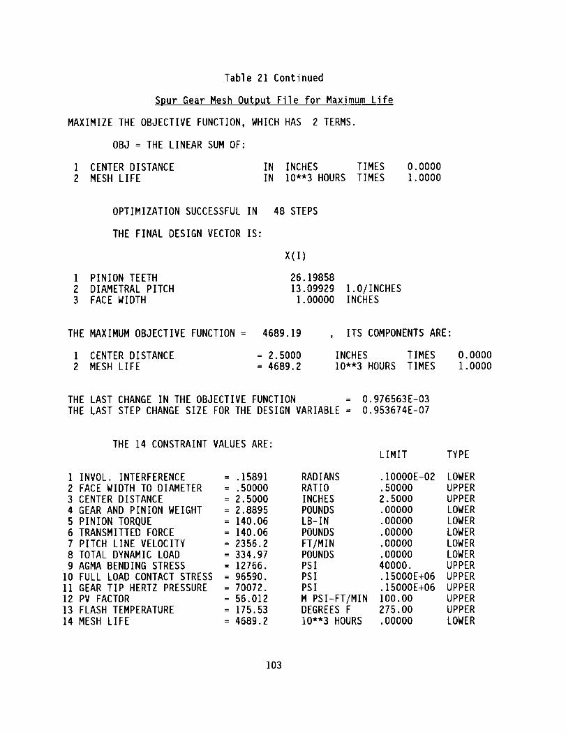
Table 2] Continued
Spur Gear Mesh Output File for Maximum Life
MAXIMIZE THE OBJECTIVE FUNCTION, WHICH HAS 2 TERMS.
OBJ = THE LINEAR SUM OF:
I CENTER DISTANCE IN INCHES TIMES
2 MESH LIFE IN 10"'3 HOURS TIMES
0.0000
1.0000
OPTIMIZATION SUCCESSFUL IN
THE FINAL DESIGN VECTOR IS:
48 STEPS
X(1)
I PINION TEETH 26.19858
2 DIAMETRAL PITCH I3.09929 ].O/INCHES3 FACE WIDTH 1.00000 INCHES
THE MAXIMUM OBJECTIVE FUNCTION =
I CENTER DISTANCE
2 MESH LIFE
4689.19 , ITS COMPONENTS ARE:
= 2.5000 INCHES TIMES
= 4689.2 10"'3 HOURS TIMES
0.00001.0000
THE LAST CHANGE IN THE OBJECTIVE FUNCTION = 0.976563E-03
THE LAST STEP CHANGE SIZE FOR THE DESIGN VARIABLE = 0.953674E-07
THE 14 CONSTRAINT VALUES ARE:
I INVOL. INTERFERENCE
2 FACE WIDTH TO DIAMETER
3 CENTER DISTANCE
4 GEAR AND PINION WEIGHT
5 PINION TORQUE6 TRANSMITTED FORCE
7 PITCH LINE VELOCITY
8 TOTAL DYNAMIC LOAD
9 AGMA BENDING STRESS
10 FULL LOAD CONTACT STRESS
II GEAR TIP HERTZ PRESSURE
12 PV FACTOR
13 FLASH TEMPERATURE
14 MESH LIFE
LIMIT TYPE
= .15891 RADIANS .I0000E-02 LOWER
= .50000 RATIO .50000 UPPER
= 2.5000 INCHES 2.5000 UPPER
= 2.8895 POUNDS .00000 LOWER
= 140.06 LB-IN .00000 LOWER
= 140.06 POUNDS .00000 LOWER
= 2356.2 FT/MIN .00000 LOWER= 334.97 POUNDS .00000 LOWER
= 12766. PSI 40000. UPPER= 96590. PSI .15000E+06 UPPER
= 70072. PSI .15000E+06 UPPER
= 56.012 M PSI-FT/MIN 100.00 UPPER= 175.53 DEGREES F 275.00 UPPER
= 4689.2 10"'3 HOURS .00000 LOWER
I03

Table 21 Continued
Spur Gear Mesh Output File for Maximum Life
DESIGN CHECK
I PINION TEETH
2 DIAMETRAL PITCH
3 FACE WIDTH
X(1)
24.00000
12.000001.00000
1.O/INCHESINCHES
THE MAXIMUM OBJECTIVE FUNCTION = 4432.67 , ITS COMPONENTS ARE:
! CENTER DISTANCE = 2.5000
2 MESH LIFE = 4432.7
INCHES TIMES 0.0000
10"'3 HOURS TIMES 1.0000
THE 14 CONSTRAINT VALUES ARE:LIMIT TYPE
I INVOL. INTERFERENCE
2 FACE WIDTH TO DIAMETER
3 CENTER DISTANCE
4 GEAR AND PINION WEIGHT
5 PINION TORQUE6 TRANSMITTED FORCE
7 PITCH LINE VELOCITY
8 TOTAL DYNAMIC LOAD
9 AGMA BENDING STRESS
10 FULL LOAD CONTACT STRESS
11 GEAR TIP HERTZ PRESSURE
12 PV FACTOR
13 FLASH TEMPERATURE
14 MESH LIFE
= .14243
= .50000
= 2.5000
= 2.8895
= 140.06
= 140.06
= 2356.2
= 334.97
= 12009.
= 97085.
= 73216.= 63.518
= 180.12
= 4432.7
RADIANS .I0000E-02 LOWERRATIO .50000 UPPER
INCHES 2.5000 UPPER
POUNDS .00000 LOWER
LB-IN .00000 LOWER
POUNDS .00000 LOWER
FT/MIN .00000 LOWERPOUNDS .00000 LOWER
PSI 40000. UPPER
PSI .15000E+06 UPPER
PSI .15000E+06 UPPER
M PSI-FT/MIN 100.00 UPPERDEGREES F 275.00 UPPER
10"'3 HOURS .00000 LOWER
]04

For this new objective of maximizing the life of a larger gear set, the
program found an optimum design with a life of 4.69 million hours in 48 steps.
This design was bounded by the center distance limit of 2.5 inches and the
length to diameter ratio limit of 0.5. This optimum also had an unrealistic
number of teeth on the pinion of 26.2 and diametral pitch of 13.1. The last
page of Table 21 shows the results of a nearby design check using 24 teeth on
the pinion, a diametral pitch of 12 and a face width of one inch. This design
is shown in Figure 16 with 24 teeth on the pinion and 36 teeth on the gear and
the requested 2.5 inch center distance.
The realistic design has a slightly lower life of 4.43 million hours, a
gear and pinion weight of 2.9 pounds, a pinion torque of ]40 pound-inches, a
transmitted force of 140 pounds, a pitch line velocity of 2356 feet per
minute, and an estimated dynamic load of 335 pounds. Since it is larger than
the minimum size design, it also has lower loads and stresses.
I05

C = 2.5"
PINION
24 TEETH
GEAR
36 TEETH
MAXIMUM LIFE SPUR GEAR DESIGN
FIGURE 1 6
106

WEIBULL DATA FITTING
The fourth example application is the use of the optimizer to fit
experimental life data to a two-parameter Weibull distribution. With its
abilities to iterate in n independent variables and provide an easy check of
the performance of alternate solutions, the computer program SEEK.FOR offers a
variety of uses. One valuable application is that of fitting a curve to
experimental data.
Theor_
A nonlinear least squares fitting procedure compares the measured data
to the fitted curve at each point. The sum of the squares of the errors
between the measured data and the values on the fitted curve is a positive
definite scalar measure of the scatter of the data about the curve. Taking
the square root of this squared error sum divided by the number of data points
less one gives a dispersion with the same dimension as the measured quantity
[22]. For the two-parameter Weibull relationship of equation (33), this
dispersion would be:
OD = ( (Rc - RD)2 11/2 (38)
ND - I
where RC is the reliability on the curve, RD is the median rank reliability of
the measured life and ND is the number of data points.
Thus one can use SEEK.FOR to determine the ninety-percent reliability
life, _I0' and Weibull slope, b, from a set of life test data. Table 22
summarizes this problem in the design optimization format with: the lone
constant being the number of data points; the two design parameters, _I0 and
]07

Table 22
Spur Gear Mesh Optimization Parameters
Constants
ND
Design Parameters
tlO
b
Inequality
ND > 0
Constraints Objective Function
(°D)min
Table 23
Median Ranked Life Data
Life
103
190
250
310
340
410450
510
550
600
670
710
770
79O
830
880
Hours
.0
.0
.0
.0
.0
.0
.0
.0
.0
.0
.0
.0
.0
.0
.0
Reliability
0.95484
0.89060
0.82568
0.76061
0.69548
0.63033
0.56517
0.500000.43483
0.36967
0.30452
0.23939
0.17432
0.10940
0.04516
108

b; the inequality constraint of having a positive number of data points; and
the objective function of minimizing the dispersion, oD.
For a group of identical units subjected to an identical life test,
different units will fail at different times. By recording the times to
failure and ranking them from the shortest to the longest, one can use a
median rank table [23] to list the median reliability and test life in a table
or data file similar to the numerical values in Table 23. This table lists
the time to failure and the corresponding median reliability for a life test
of fifteen units.
Proqramminq
Inside SEEK.FOR is the additional capability to read a second data file
in addition to the input data file. This action is enabled by setting the
first constant in the constant array to the number, n, of data point pairs,
(XDi,YDi), in the data file and including the words, "DATA POINTS," in its
description. When this is combined with the presence of a data file of n
lines with n point pairs; XD i , YDi; and a name which has the same prefix as
the ".IN" file but the extension ".DAT;" SEEK will open and read the ".DAT"
file after it has read the ".IN" file. The data pairs will be placed in a
common block, COMMON/CURVE/XDP(2OO),YDP(200), for use in subroutine VALUES.
If the limit of 200 data pairs is too low, changing this dimension in the
program will allow larger data sets to be fit.
Table 24 lists subroutines BOUNDS and VALUES which will fit a two-
parameter Weibull distribution to the data in the ".DAT" file. Subroutine
BOUNDS checks that the number of data points is positive, since it has to do
something to permit the overall program to execute. Subroutine VALUES uses
109
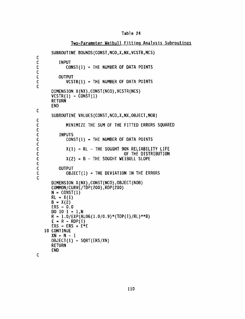
C
C
C
C
C
C
C
C
C
C
C
C
C
C
C
C
C
C
C
C
C
Table 24
Two-Parameter Weibull Fittinq Analysis Subroutines
SUBROUTINE BOUNDS(CONST,NCO,X,NX,VCSTR,NCS)
INPUT
CONST(1) = THE NUMBER OF DATA POINTS
OUTPUT
VCSTR(1) = THE NUMBER OF DATA POINTS
DIMENSION X(NX),CONST(NCO),VCSTR(NCS)VCSTR(1) = CONST(1)RETURN
END
SUBROUTINE VALUES(CONST,NCO,X,NX,OBJECT,NOB)
MINIMIZE THE SUM OF THE FITTED ERRORS SQUARED
INPUTS
CONST(I) = THE NUMBER OF DATA POINTS
X(1) = RL - THE SOUGHT 90% RELIABILITY LIFEOF THE DISTRIBUTION
X(2) = B - THE SOUGHT WEIBULL SLOPE
OUTPUT
OBJECT(1) = THE DEVIATION IN THE ERRORS
DIMENSION X(NX),CONST(NCO),OBJECT(NOB)
COMMON/CURVE/TDP(2OO),RDP(200)
N = CONST(1)
RL = X(I)
B = X(2)ERS = 0.0
DO 10 I = I,N
R = I.O/EXP(ALOG(].O/O.9)*(TDP(1)/RL)**B)
E = R - RDP(1)ERS = ERS + E*E
10 CONTINUE
XN = N - I
OBJECT(]) = SQRT(ERS/XN)RETURN
END
110

equations (33) and (38) to determine the dispersion of the measured data about
the trial distribution.
Numerical Example
To illustrate this data fitting process, the fifteen data points of
Table 23 and the analysis subroutines of Table 24 will be used. A listing of
the input data file "W.IN" which will initiate the curve fitting is given in
Table 25. In this file; the first line is the problem title; the second line
is the number of constants, which is one; and the next three lines are the
number of data points, 15; the description "NUMBER OF DATA POINTS" which
includes the words "DATA POINTS" and a blank line for the units. Following
this is a line with the number of independent parameters, two. The next six
lines give the two distribution parameters, with their low, high and initial
estimates. This is followed by the number of design constraints, one, and
three lines which describe the lower bound on the number of data points. On
the next line are the three letters "MIN" to signal that the objective
function is to be minimized and four lines which give the number of object
functions as one and the weighting coefficient, description and units for the
reliability error dispersion. Once again, the unit line is blank.
Compiling the subroutines of Table 24, linking them with SEEK.OBJ, and
running the resulting program with the two data files W.DAT which holds the
numbers of Table 23 and W.IN which is listed in Table 25 yields the output
file of Table 26. This file echoes the input file information and reports a
successful curve fit in 43 steps. The fitted curve has an _IO life of
238.8 thousand hours and a Weibull slope of 2.296 with a dispersion
reliability of 0.0317.
lll
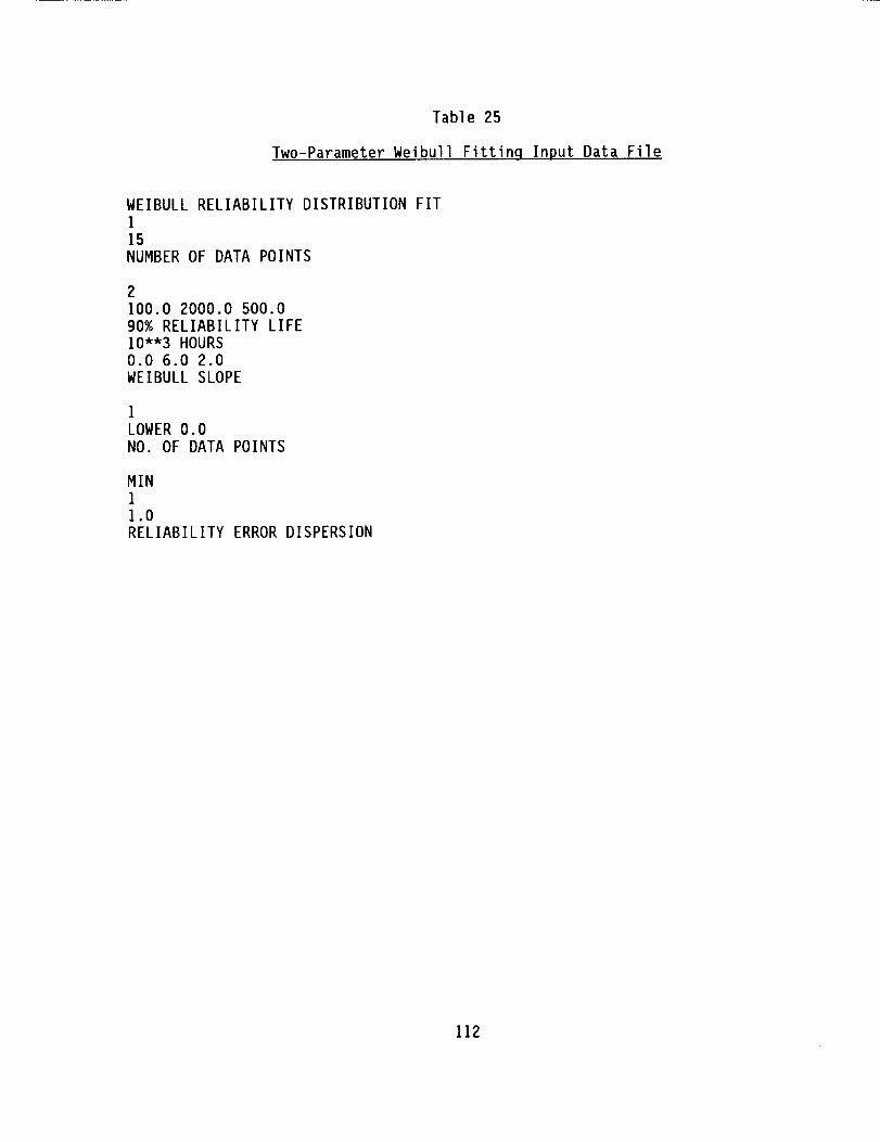
Table 25
Two-Parameter Weibull Fittinq Input Data File
WEIBULL RELIABILITY DISTRIBUTION FIT
I
15NUMBER OF DATA POINTS
2
100.0 2000.0 500.0
90% RELIABILITY LIFE10"'3 HOURS
0.0 6.0 2.0
WEIBULL SLOPE
I
LOWER O.0
NO. OF DATA POINTS
MIN
I
1.0
RELIABILITY ERROR DISPERSION
112
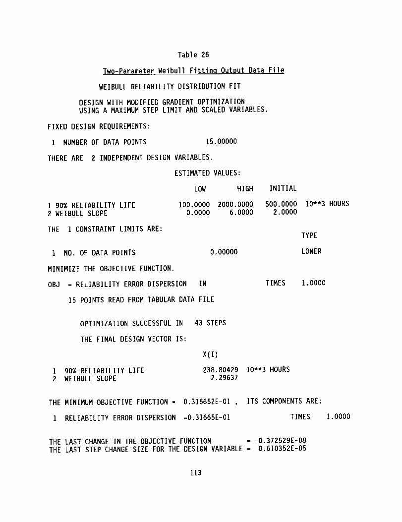
Table 26
Two-Parameter Weibull Fittinq Output Data File
WEIBULL RELIABILITY DISTRIBUTION FIT
DESIGN WITH MODIFIED GRADIENT OPTIMIZATION
USING A MAXIMUM STEP LIMIT AND SCALED VARIABLES.
FIXED DESIGN REQUIREMENTS:
I NUMBER OF DATA POINTS 15.00000
THERE ARE
I 90% RELIABILITY LIFE
2 WEIBULL SLOPE
2 INDEPENDENT DESIGN VARIABLES.
ESTIMATED VALUES:
LOW HIGH
100.0000 2000.0000
0.0000 6.0000
THE I CONSTRAINT LIMITS ARE:
INITIAL
500.0000
2.0000
I NO. OF DATA POINTS
MINIMIZE THE OBJECTIVE FUNCTION.
OBJ = RELIABILITY ERROR DISPERSION IN
15 POINTS READ FROM TABULAR DATA FILE
0.00000
TIMES
10"'3 HOURS
TYPE
LOWER
1.0000
OPTIMIZATION SUCCESSFUL IN
THE FINAL DESIGN VECTOR IS:
l 90% RELIABILITY LIFE
2 WEIBULL SLOPE
43 STEPS
X(1)
238.80429
2.29637
10"'3 HOURS
THE MINIMUM OBJECTIVE FUNCTION = 0.316652E-01 , ITS COMPONENTS ARE:
I RELIABILITY ERROR DISPERSION =0.31665E-01 TIMES 1.0000
THE LAST CHANGE IN THE OBJECTIVE FUNCTION = -0.372529E-08
THE LAST STEP CHANGE SIZE FOR THE DESIGN VARIABLE = 0.610352E-05
113

Table 26 Continued
Two-Parameter Weibull Fittinq Output Data File
THE I CONSTRAINT VALUES ARE:
I NO. OF DATA POINTS = 15.000
LIMIT
.00000
TYPE
LOWER
DESIGN CHECK
I 90% RELIABILITY LIFE
2 WEIBULL SLOPE
X(1)
240.00000
2.30000
THE MINIMUM OBJECTIVE FUNCTION = 0.315955E-01 ,
I RELIABILITY ERROR DISPERSION =0.31596E-01
THE I CONSTRAINT VALUES ARE:
I NO. OF DATA POINTS = ]5.000
10"'3 HOURS
ITS COMPONENTS ARE:
TIMES
LIMIT
.00000
1.0000
TYPE
LOWER
114
As shown in the design check, rounding the £10 life to 240 thousand
hours and the Weibull slope to 2.3 changes this dispersion to 0.0316. This
rounded function fits the data slightly better than the "ideal" function as
found by the optimizer due to the finite step size procedure of the gradient
algorithm. Selecting a different starting position or sensitivity ranges for
the two Weibull parameters could result in an "ideal" solution which is
slightly better than the rounded solution, but it would not be significantly
different. A good fit is achieved with two digit precision parameters, using
the combination of the optimizer and the design check.
Figure 17 is a two-parameter Weibull graph of the measured data with its
median rank reliability plotted as crosses. On this plot is drawn the rounded
two-parameter Weibull distribution which has been fit to the data. It is
always a good idea to draw the fitted curve with the data points to which it
is fit. Since the dispersion is a single value representing the overall fit
of the curve, some local anomalies may exist in a fitted curve. A graph shows
these. If the data does not have the general shape of the fitted function,
either a partial fit in the region of interest or a more sophisticated
function should be used.
By changing the ranking from median to both low and high reliability
ranks, the program can be run twice more to determine confidence bounds on the
distribution. These two runs would give the user a low reliability fit to the
test data and a high reliability fit to the same data. Plotting these two
curves on the graph of Figure 17 would show the confidence range for the
distribution.
To investigate the potential improvement in fitting the data with a
higher order Weibull distribution, a three-parameter Weibull distribution
115

RELIABILITY- R (, % )
1.0
5.010.0
20.0
50.0
90.0
95.0
m
m
u
m
i99.0
100 .0
++
m
I I I I I I 1 I I
200.0 500.0 1,000.0
LIFE - ( 10 3 HOURS )
TWO-PARAMETER WEIBULL DISTRIBUTION
WITH t,10 = 240 * 10 3 HOURS AND b = 2.3
FIGURE 17
116
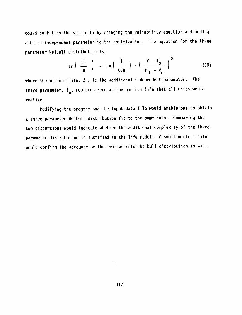
could be fit to the same data by changing the reliability equation and adding
a third independent parameter to the optimization.
parameter Weibull distribution is:
The equation for the three
b
Ln [ 1 1 _ - _o
R 0.9 _I0- _o
where the minimum life, _o' is the additional independent parameter. The
third parameter, _o' replaces zero as the minimum life that all units would
realize.
Modifying the program and the input data file would enable one to obtain
a three-parameter Weibull distribution fit to the same data. Comparing the
two dispersions would indicate whether the additional complexity of the three-
parameter distribution is justified in the life model. A small minimum life
would confirm the adequacy of the two-parameter Weibull distribution as well.
117

OPTIMIZATION METHOD
Parameter Scalinq
As illustrated in the examples, the optimization procedure begins with
several vectors. An optimization solution is the design variable vector, X,
which minimizes or maximizes the objective function value, M, with all
constraint values, Vk, bounded by their specified limits. A procedure starts
with a guess for the design variables, X, and iterates using gradients to find
the optimal values. Opportunity is then given to the user to try alternate
solutions and compare their properties.
To maintain balance among the independent design parameters, the design
space is scaled into a dimensionless design space [3]. The scaled design
parameters, Yi' vary from - 1.0 to + I.O as specified by upper and lower
bounds on the independent design parameters, X
as
such that:i'
- 1.0 < Y. < + 1.0 (40)1
XLi < Xi < XUi (41)
This linear transformation, which is shown in Figure 18, is:
where
Yi : di Xi + bi (42)
and
d. = (43)l
XUi - XLi
Xui + XLi
bi = - (44)
XUi - XLi
118

y.
I
0
bi
-1
XLi
di
XUi X •
I
DESIGN PARAMETER
TRANSFORMATION
SCALING
FIGURE 18
119

The actual design variable, Xi, can be retrieved from the scaled variable, Yi'
by the inverse transformation:
X °
l
_ Yi - bi (45)
di
Gradients
Central to this method is the gradient calculation which is performed
with small perturbations in the design variables from the nominal position.
The gradient in the merit function, VM, is calculated {I] as:
VM (46)
where,
aM M(YI'"Yi+AY'"Yn) - M(YI'"Yi'"Yn) (47)
: AY
In the program, the small change AY, which is made in each Yi' is set at 0.001
which is 0.05 percent of the full range of a scaled design parameter.
The magnitude of the gradient vector is given by:
120

vMl;(Z:(aM
i=! _Yi
2 i/2
(48)
In the program, the step size is separated from the gradient magnitude but for
minimization its direction is opposite to the gradient direction, so negative
unit gradient vectors are determined:
VM
V m = (49)
JVMI
For maximization, the sign in equation (49) reverses. This sign reversal
also occurs for the constraint gradient when the limit is a lower bound.
Search Directions
In the simple gradient method which is used in the acceptable design
region, equation (49) defines the direction of change in the scaled design
vector, Yj.
Yj+I = Yj + _S • Vm (50)
If no constraints are violated, this will be the next value for Yj in the
search.
For stability and directness, a nominally fixed step size, /t_, is used
in this optimization. Initially, the step size is 0.1, which is five percent
of the range of a single design parameter. Then, whenever a local minimum is
reached or the search is trapped in a constraint corner, the procedure halves
the step. To complete the search procedure, the program declares a solution
121

when the percent change in the merit function is less than a pre-set limit of
0.0001:
Mj+ I - Mj < 0.0001 (51)
M.3
Two other modes of searching are used in the procedure: I) poor guess
correction when constraints are violated initially, and 2) feasible direction
searching near constraint boundaries.
These modes are enabled with a second gradient. Just as one can
calculate the gradient in the objective function, one also can calculate the
gradient in a violated constraint variable:
V Vk (52)
VVk = I VV k I
For upper bound constraints, moving through the design space in the direction
of V vk will reduce the constraint value Vk. For lower bound constraints, a
sign reversal in equation (52) produces an increase in the constraint value,
for motion in the gradient direction. The vector sum of the gradients inVk,
the violated constraints, V h, is the second gradient of the algorithm:
Vv k
kV h = (53)
vVklk
The gradient in the violated constraints, V h, points towards the
acceptable design space from the unacceptable design space. By itself, it
122

enables the algorithm to turn an unacceptable initial guess into an acceptable
design trial by a succession of steps:
Yj+I : Yj + AS' V h (54)
Once inside the acceptable design region, the algorithm proceeds along
the steepest descent direction with equation (50) until the calculated step
places the next trial outside the acceptable design space. To avoid this
condition, the algorithm selects a feasible direction for the next step.
Figure 19 shows a sloped constraint intersecting vertical contour lines of the
objective function. This figure is an enlargement of a small region in
Figure 2, which is a plot of the length versus diameter for a bushing. In
this example, the objective function is directly proportional to the bushing
diameter and independent of its length. So a steepest descent direction is
always horizontal for the problem. The sloped constraint curve is the length
to diameter upper bound. Figure 19 showsvertical contour lines in the
frictional torque objective function and unit gradient vectors in this
objective function, Vm, and the impending constraint, V h. The two gradient
vectors are added at the last viable design step. The feasible direction
selected, V f, is the unit vector sumof these two gradients:
Vm+VhV f : (55)
IVm+Vh I
And the next step becomes:
Yj+I = Yj + AS • V f (56)
123
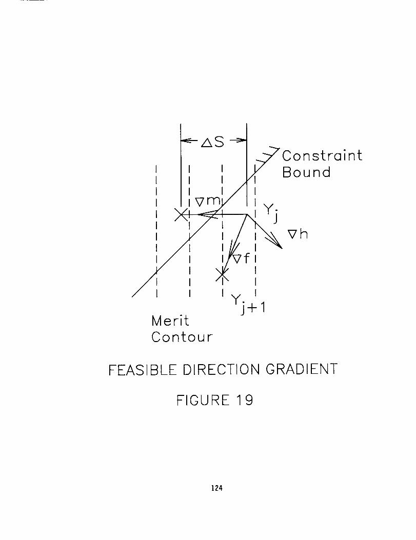
_-/xS -->
MeritContour
ConstrointBound
FEASIBLE DIRECTION GRADIENT
FIGURE 1 9
124
Proqram Structure
In writing the optimization code, subroutines were used to modularize
the programming and perform the vector calculations in a structured way.
Table I, which is cited in the PROGRAMMING section of this report, lists the
subroutines which compose this program with short descriptions of their
functions. Each subroutine's name is related to its operation to describe its
use.
The scaling and unscaling of the design parameter vector are performed
by two routines: SIZE and RESIZE, so that this linear transformation can be
performed anywhere in the program with relative ease. Subroutines GRADNT and
UNIT evaluate and normalize any gradient vector. Subroutine BOUNCE finds the
gradient sum of the violated constraints at any design position. Subroutine
CHECK compares a constraint value to its limit and subroutine WALL evaluates a
specific constraint in the same way that subroutine MERIT evaluates the
objective function.
At a higher level in the program structure, subroutine BOUNCE directs
the search for the acceptable design space when the initial design guess
violates at least one constraint. Subroutine SCAN performs the search for
better designs within the acceptable design space and subroutine SCOUT checks
the next potential design for constraint violations. Finally, subroutines
BOUNDS and VALUES are the user supplied, problem specific routines which
evaluate the design constraints and the objective function values for the
design.
Figure 20 is a logic flow chart for the optimization program which
includes: I) the reading of the input data files, 2) the echoing of the input
data file information at the start of the output data file, 3) the initial
125

I READDATA& SETCONSTANTS IWRITEINPUT DATATO OUTPUTFILEI
I
I FOR FIRST CONSTANT OF "DATA POINTS" IREAD TABLE OF XDP. YDP VALUES I
ICHECK CONSTRAINT & MERIT FUNCTION VALUESl
IIARE ALL CONSTRAINTS SATISFIED ?J
yes !
CALCULATE Vm & LOCATION OF NEXT POINTALONG Vm & CONSTRAINT VALUE THERE
IARE ALL CONSTRAINTS SATISFIED ?I
no
no
ITAKE STEP IN Vm DIRECTIONI
I DID MERIT FUNCTION IMPROVE ?
DID MERIT FUNCTION BECOME ZERO ?IS ITS PERCENT CHANGE SMALL ?
OR HAVE 500 TRIALS BEEN MADE ?
JMOVE ALONG Vhl
7"I"OA NEW POINTI
yes IWRITE FOUND DESIGN AND ITS PROPERTIESI
1IOFFER CHANCE TO CHANGE DESIGNI
y°81IACCEPT NEW DESIGN PARAMETER VALUESI
[ANALYZE DESlGNI
-i CALCULATE Vfl
IS AT IA#E EAL L#T O##TR A/N TSSTEP? I no
ITAKE STEP IN Vf DIRECTION II
no
no
no
SEEK PROGRAM FLOW CHART
FIGURE 20
126

search for a good starting design, 4) the main optimization loop, and 5) the
design verification loop.
The search for a good starting design which satisfies all constraints is
performed in a DOloop with a limit of twenty corrections. If a valid design
is not found in twenty trials, both the first and twentieth trials are written
to the output file with an analysis of all constraints, the file is closed and
the program is stopped.
Once a good starting design is found, the search for the optimal design
is conducted in the main DOloop with a limit of five-hundred iterations. In
this DOloop, subroutine SCOUTchecks the constraint values at the next design
point using the objective function gradient increment as shown in
equation (50) to locate the next design point. If all the constraints are
satisfied, the full design step is taken in the direction of the objective
function gradient using equation (50). If at least one constraint is not
satisfied, subroutine SCANincrements the design along the feasible direction
gradient using equation (56). If all the constraints are still not satisfied,
the step size is reduced and the half step is taken in the feasible direction.
After a step is taken, the objective function value is then checked. If
it increased, the step size is divided by two. Otherwise, no change is made.
Finally, the percent change in the objective function is checked using MERIT.
If this change is below the desired limit, a solution is declared and the
procedure leaves the DOloop. If the change is greater than the desired
limit, the DOloop indexes and the iteration process is repeated.
If the merit function criteria are not satisfied after five-hundred
iterations, the program writes the five-hundredth design to the screen and the
output file with an error messageand provides the user with the opportunity
127
to change the design and have it re-analyzed. This documentation and
opportunity for modification are also given to the user at the end of a
successful design optimization search. The final design modification loop is
controlled by the user with no termination count. Additional designs maybe
evaluated until the user chooses to end the program.
128
DISCUSSIONOF RESULTS
In this report, a computer program, 'SEEK.FOR,' is described and its use
is illustrated with four different examples. SEEKhas been written to make
optimization available to the general technical community with only the need
for modeling the applied problem. The program is a general purpose optimizing
tool which can find the best combination of design parameter values which
satisfy a series of constraints placed on calculable properties of the design
parameters. The set of design parameter values is 'best' in that it maximizes
or minimizes a linear sumof objective function terms.
Although the computer program requires the user to write two analysis
subroutines and an input data file for his or her application, it is written
to be interactive and to communicateclearly to the user. By requiring text
labels for all variables, the program is able to label its restatement of the
problem and all results in the words of the user. In the input file, the user
is able to change the starting design values and the relative sensitivity of
the individual design parameters by changing the low and high estimates of
these values.
Based on a boundedstep gradient method, the program searches with
gradients in three functions: ]) the objective function, 2) the violated or
nearly violated constraints and 3) a vector sumof the first two. The first
gradient provides a rapid solution path whenno obstacles are present. The
second gradient permits the user to start with an initial trial design which
maynot satisfy all constraints. And the third gradient allows the algorithm
to continue improving the objective function even whenthe direct path is
blocked with one or more constraints.
129

To enable the gradient calculations, the provided models for the
objective function terms and the constrained variables need to be continuous.
Discrete values can be entered later in a design check modewhich the program
enters once a numerical optimum has been found in the continuous design space.
This design check modeis part of the interactive operation of the program.
By allowing the user to try alternate designs after the numerical optimum has
been found, the program assists the user in finding practical optimums which
satisfy discrete requirements which can not be treated in the continuous
models. An output file is written during the session to document the design
problem and all solutions which are displayed on the screen. In this file,
each solution has its design parameter values, objective function values, and
constrained variable values and limits listed with the users descriptions as
labels.
This report illustrates the model preparation and programming required
to use 'SEEK.FOR'for four examples: I) a bushing design, 2) a spring design,
3) a gear design, and 4) a curve fit. The bushing design problem illustrates
the determination of two parameters: the bushing length and its diameter
subject to three inequality constraints, a single objective function and
discrete size requirements. The example also shows the program's ability to
overcome a poor initial trial design.
The spring design problem illustrates the conversion of equality
constraints to simplify the problem by taking a four-parameter problem and
treating it as a problem with two independent parameters. The number of
active coils in the spring and the free length of the spring are shownto be
dependent parameters and the wire diameter and meancoil diameter are left as
independent parameters. The example finds three separate designs which all
130

have the samestiffness and design factor under the sameloading but which
satisfy three separate objective functions. By changing the objective
function for the samedesign constraints, the program finds the lightest
spring, the smallest volume spring and the shortest spring in separate runs.
A visual comparison of the three springs showstheir obvious differences.
The gear design problem illustrates a three parameter design problem
which requires considerably more analysis than the first two. The three
parameters are the numberof teeth on the pinion, the diametral pitch and the
face width of the gears. Designs are obtained for a minimumsize at a given
life and for a maximumlife at a given size. The example illustrates the use
of additional subroutines by the two analysis routines: BOUNDSand VALUES.
The curve fit problem illustrates the use of the optimizing program as a
tool for minimizing the dispersion of the data from a modeled function.
Although the program can minimize the overall error between a fitted curve and
the experimental data, it is recommendedthat a plot of the fitted curve and
the original data be madeto verify that the function truly models the data
closely in the region of highest interest. One feature of this use of the
program is the ability in the design check modeto quickly see the influence
of curve coefficients on the goodness of fit.
No optimization program can solve all problems. The use of this program
is limited to solving problems which can be modeled continuously with finite
constraint and objective function values over the search area. The program
contains arbitrary size limits of forty for the constants and constraints and
fifteen for the design parameters and objective function terms. As the number
of independent design parameters increases from the low numbers of these
examples, gradient searching becomesmore difficult. More steps are required
131
to find a solution and more calculations are required for each step. Design
parameters, which do not change, can dilute the effectiveness of the method
with additional calculations. Often, a large optimization problem can be
reduced to a simpler one which permits a more rapid and direct solution by the
removal of design parameters which do not change from the design parameter
vector.
For any problem which can be modeled continuously, the program
'SEEK.FOR' offers an easily used, interactive tool for the determination of a
practical optimum solution. The program is small with an object code size of
46 k bytes and runs quickly on a 486 personal computer running DOS.
132

SUMMARYOFRESULTS
In this report, the use of a computer program, 'SEEK.FOR'is
demonstrated with four optimization examples. The program is written to work
with two user-provided subroutines and an input data file. Its purpose is to
perform a gradient search optimization of a user's problem. The method of
optimization uses a modified feasible directions gradient in addition to
simpler gradients in the objective function and the violated constraints. The
program is written in ANSI standard Fortran 77, is about ],200 lines long and
has an object size of about 46 K bytes for the optimizing code for use on a
personal computer running DOS.
To illustrate the use of the program, this report documents four
optimization examples: a bushing design, a helical coil spring design, a gear
meshdesign and a two-parameter Weibull life-reliability _urve fit. In each
example, the theory of the problem is described, the organization of the
problem into an optimization framework is given, the programming of the
modeling subroutines is explained and a numerical example is shownwith the
input and output data files explained.
In the bushing design problem, two independent design parameters are
found which minimize a single objective function subject to three inequality
constraints. In the spring design problem, four design parameters are reduced
to two independent design parameters and three separate objective functions
are minimized with three separate runs of the sameprogram. The designs
satisfy seven inequality constraints. For the gear design problem, two sets
of three independent design parameters are found in two separate runs to
satisfy two opposing objective functions. In this model, fourteen inequality
constraints are satisfied. For the curve fitting example, a table of x and y
133

data points is read into the program and two parameters are found which fit a
curve to the data with minimized dispersion. One innocuous inequality
constraint is used to allow the program to run, since the program requires the
subroutine to be in place. As written, the program accepts problems with up
to forty input data constants and forty inequality constraints. The limit on
the number of independent design parameters is fifteen as is the limit on the
number of objective function terms.
This report describes the use of the optimizing program, gives four
examples of its use and discusses the program and method themselves. The
program 'SEEK.FOR'is an adaptable, analytical tool for finding optimal
solutions to technical problems.
134

APPENDIXA
SEEK.DOCFILE
CCCCCCCCCCCCCCCCCCCCCCCCCCCCCCCCCCCCCCCCCCCCCCCC
PROGRAMSEEK.FOR
MODIFIEDGRADIENTOPTIMIZATIONPROGRAM
WITHINEQUALITYCONSTRAINTAVOIDANCE
LINK THIS PROGRAMWITHTWOPROBLEMSPECIFICANALYSISSUBROUTINESANDRUNWITHA PROBLEMSPECIFICDATAFILE.
"NAME".IN DATAINPUTFILE REQUIRED
FORMAT:
LINE I : NTITLE(50 CHAR.MAX)FORTHECONSTANTS
LINE 2 : NCOIN SETSOFTHREELINESEACH
LINE 3 - (IA) : CONST(1)LINE 4 - (2A) : NCON(30 CHAR.MAX)LINE 5 - (3A) : NUCON(12 CHAR.MAX)
THENFORTHEINDEPENDENTVARIABLESLINE 3 + 3*NCO : NX
IN SETSOFTHREELINESEACHLINE (IB) : XLOW(1), XHIGH(1) , XZ(1)LINE (2B) : NVAR(30 CHAR.MAX)LINE (3B) : NUVAR(12 CHAR.MAX)
THENFORTHECONSTRAINTSLINE 4 + 3*NCO+ 3*NX : NCS
IN SETSOFTHREELINESEACHLINE (IC) : LIMIT(1) , CSTR(1)LINE (2C) : NCSTR(30 CHAR.MAX)LINE (3C) : NUCSTR(]2 CHAR.MAX)
THENFORTHEOBJECTIVEFUNCTIONLINE 5 + 3*NCO+ 3*NX+ 3*NCS : DIRLINE 6 + 3*NCO+ 3*NX + 3*NCS : NOB
IN SETSOFTHREELINESEACHLINE (ID) : WGHTF(1)LINE (2D) : NOBJ(30 CHAR.MAX)LINE (3D) : NUOBJ(12 CHAR.MAX)
TOHAVEACCESSTOA TABLEOFX ANDY DATAVALUES,LET THEFIRSTCONSTANTBE THENUMBEROFDATAPOINTSANDINCLUDETHEWORDS"DATAPOINTS"IN ITS DESCRIPTION.
A DATAFILE WITHX,Y DATAPAIRSANDTHENAME"NAME".DATSHOULDALSOEXIST IN THESAMEDIRECTORY.
135

UPTO 200 DATAPAIRSWILL BE PLACEDIN THECOMMONBLOCKCOMMON/CURVE/XDP(2OO),YDP(200).
TWO ANALYSIS SUBROUTINES ARE REQUIRED
BOUNDS(CONST,NCO,X,NX,VCSTR,NCS) ; ANDVALUES(CONST,NCO,X,NX,OBJECT,NOB)
BOUNDS EVALUATES THE INEQUALITY CONSTRAINTS
VALUES DETERMINES THE OBJECTIVE FUNCTION'S
COMPONENT PROPERTIES
DEFINITIONS:
CONST
CSTR
DIR
LIMIT
NCONCS
NOB
NX
NCON
NUCONNVAR
NUVAR
NCSTR
- FIXED DESIGN PROBLEM CONSTANT- CONSTRAINT LIMIT VALUE INCLUDING DECIMAL POINT
- OPTIMIZATION DIRECTION ( MIN , MAX )
- CONSTRAINT LIMIT BOUND TYPE ( UPPER , LOWER )- NUMBER OF PROBLEM CONSTANTS
- NUMBER OF INEQUALITY CONSTRAINTS- NUMBER OF PROPERTIES IN MERIT FUNCTION
- NUMBER OF INDEPENDENT VARIABLES
- CONSTANT NAME
- CONSTANT DIMENSION UNITS- VARIABLE NAME
- VARIABLE DIMENSION UNITS
- CONSTRAINT NAME
NUCSTR - CONSTRAINT DIMENSION UNITS
NOBJ - MERIT FUNCTION COMPONENT NAMENUOBJ - MERIT FUNCTION COMPONENT DIMENSION UNITS
NTITLE - DESIGN PROBLEM TITLE
OBJECT - MERIT FUNCTION COMPONENT VALUES
VCSTR
WGHTF
X
XHIGH
XLOW
XZ
- CONSTRAINT FUNCTION VALUES
- WEIGHTING COEFFICIENT FOR COMPONENT IN
LINEAR MERIT FUNCTION SUM
- INDEPENDENT DESIGN VARIABLE
- HIGH VARIABLE VALUE
- LOW VARIABLE VALUE
- INITIAL VARIABLE VALUE
AT PRESENT, THE ARRAY SIZE LIMITS ARE:
MAX NCO = 40,
MAX NCS = 40,
MAX NOB = 15, ANDMAX NX = 15.
136

CCCCCCCCCCCcCCcCCcccCCcCCCCCCCCCCCCCCCcCCCC
AVOID THE USE OF SUBROUTINE AND COMMON BLOCK NAMES
WHICH ARE ALREADY USED BY SEEK.
THE SUBROUTINE NAMES USED BY SEEK ARE:
BACK ........... FSUBRT
BOUNCE .......... FSUBRT
BOUNDS .......... extern
CHECK .......... FSUBRTGRADNT .......... FSUBRT
MERIT .......... FSUBRT
RESIZE .......... FSUBRT
SCAN ........... FSUBRT
SCOUT .......... FSUBRT
SIZE ........... FSUBRT
UNIT ........... FSUBRT
VALUES .......... extern
WALL ........... FSUBRT
THE COMMON BLOCK NAMES USED BY SEEK ARE:
CURVE .......... common
PAR ........... common
VAR ........... common
UNITS .......... common
TO PRINT OUT INTERMEDIATE RESULTS FROM BOUNDS, VALUES
OR ANY SUBROUTINE CALLED BY BOUNDS OR VALUES, INCLUDE THE
COMMON BLOCK "UNITS" IN THAT SUBROUTINE, AS FOLLOWS:
COMMON /UNITS/NW,NR,NF,ND
WHERE:
NW = WRITE NUMBER FOR WRITING TO THE SCREEN
- WRITE(NW,...)NR = READ NUMBER FOR READING FROM THE KEYBOARD
- READ(NR,...)NF = WRITE NUMBER FOR WRITING TO THE OUTPUT FILE
- WRITE(NF,...) ,ANDND = READ NUMBER FOR READING FROM THE INPUT DATA FILE
- READ(ND,...).
137

Vari abl es
A
b.1
B
C
C2
C
Cg
Ct
d.I
d w
D
E
i
F
Vf
G
hf
Vh
J
k
Kw
R
_o
APPENDIX B
SYMBOLS
- AGMA velocity factor constant
- independent design variable scaling constant
- material surface strength constant (psi)
- center distance (in)
- minimum gear tooth curvature (in)
- dynamic capacity (Ibs)
- gear dynamic capacity (Ibs)
- tooth dynamic capacity (Ibs)
- independent design variable scaling slope
- wire diameter (mm)
- shaft or mean coil diameter (mm)
- elastic modulus (psi)
- face width (in)
- applied force (N)
- normalized feasible direction gradient
- shear modulus (MPa)
- unloaded spring height (mm)
- normalized violated constraint gradient
- polar moment of inertia (mm4) or AGMA bending stress factor
- spring rate (N/mm)
- Wahl stress concentration factor
- life (h)
- minimum life (h)
I38
_m
L
M
Vm
_M
Na
Ndes
ND
Ne
Nf
Ng
Ns
OD
P
Pd
PV
Qv
R
R
Rc
RD
Sac
Sse
SSU
Ssy
Suc
- mesh life (103h)
- bearing length (mm)
- objective function vector
- normalized objective function gradient
- unscaled objective function gradient
- number of active spring coils
- design factor
- number of data points
- number of inactive end coils
- design factor in fatigue
- number of gear teeth
- static design factor
- outside coil diameter (mm)
- contact pressure (MPa)
- diametral pitch (in-])
- pressure times velocity scoring factor (MPa - m/s)
- AGMA surface quality factor
- gear radius (in)
- reliability
- calculated reliability
- measured reliability
- surface compression strength (psi)
- shear endurance strength (MPa)
- shear ultimate strength (MPa)
- shear yield strength (MPa)
- tensile strength constant (MPa)
139
AS
TB
Tf
If
Tq
V
- step size
- base temperature (°F)
- flash temperature (°F)
- friction torque (N-m)
- applied torque (Ib-in)
- shear force (N)
Vcoil - spring coil cylinder volume (mm3)
Vk
Vw
V
Vs
Vv k
W
W
Wt
X
XD.1
XL
XU
XG
x.
XF
Y
AY
YD i
Q
- single violated constraint
- wire volume (mm3)
- pitch line velocity (ft/sec)
- sliding velocity (m/s) or (ft/sec)
- single violated constraint gradient
- weight density (kN/m3)
- gear weight (Ibs)
- spring weight (N)
- independent design parameter vector
- life test data value (]03 h)
- independent design parameter lower value
- independent design parameter upper value
- geometric temperature factor
- thermal-elastic temperature factor
- load sharing temperature factor
- scaled independent design parameter vector
- incremental step change in scaled design parameter vector
- reliability data point value
- gear tooth involute angle (radians)
140

B
6
61
0
/1
Pm
V
P
%
%
%
GHt
r
o)
- length to diameter ratio
- spring deflection (mm)
- involute interference angle (radians)
- spring wire rotation angle (radians)
- coefficient of friction
- surface roughness (RMS)
- Poisson's ratio
- radius of curvature (in)
- bending stress (psi)
- dispersion of data from fitted curve
- Hertzian contact stress (psi)
- Hertzian contact stress at the gear tooth tip (psi)
- shear stress (MPa)
- pressure angle (radians)
- gear angular velocity (rad/sec)
- shaft speed (RPM)
Subscripts
a - alternating
al - pinion addendum
a2 - gear addendum
bl - pinion base
b2 - gear base
d - dynamic
i - independent design parameter index
j - optimization step index
141
k - violated constraint index
m - mean
max - maximum
min - minimum
sol - solid height
] - pinion
2 - gear
10 - 90 percent reliability
Superscripts
a
b
P
- wire strength exponent
- Weibull slope
- load-life exponent
142
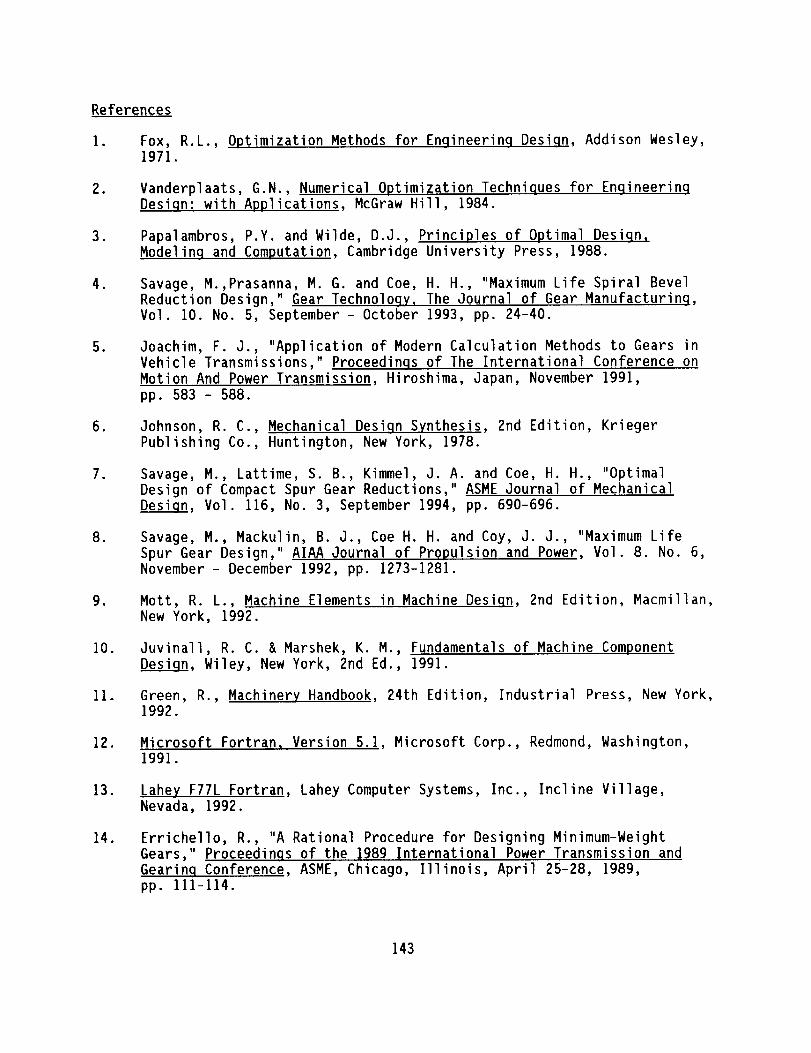
References
6 Fox, R.L., Optimization Methods for Enqineerinq Desiqn, Addison Wesley,1971.
. Vanderplaats, G.N., Numerical Optimization Techniques for Enqineerinq
Desiqn: with Applications, McGraw Hill, 1984.
. Papalambros, P.Y. and Wilde, D.J., Principles of Optimal Desiqn,
Modelinq and Computation, Cambridge University Press, 1988.
o Savage, M.,Prasanna, M. G. and Coe, H. H., "Maximum Life Spiral Bevel
Reduction Design," Gear Technoloqy, The Journal of Gear Manufacturinq,
Vol. 10. No. 5, September - October 1993, pp. 24-40.
o Joachim, F. J., "Application of Modern Calculation Methods to Gears in
Vehicle Transmissions," Proceedinqs of The International Conference on
Motion And Power Transmission, Hiroshima, Japan, November 1991,
pp. 583 - 588.
. Johnson, R. C., Mechanical Desiqn Synthesis, 2nd Edition, Krieger
Publishing Co., Huntington, New York, 1978.
° Savage, M., Lattime, S. B., Kimmel, J. A. and Coe, H. H., "Optimal
Design of Compact Spur Gear Reductions," ASME Journal of Mechanical
Desiqn, Vol. 116, No. 3, September 1994, pp. 690-696.
. Savage, M., Mackulin, B. J., Coe H. H. and Coy, J. J., "Maximum Life
Spur Gear Design," AIAA Journal of Propulsion and Power, Vol. 8. No. 6,
November - December ]992, pp. 1273-1281.
go Mott, R. L., Machine Elements in Machine Design, 2nd Edition, Macmillan,
New York, 1992.
10. Juvinall, R. C. & Marshek, K. M., Fundamentals of Machine Component
Desiqn, Wiley, New York, 2nd Ed., 1991.
11. Green, R., Machinery Handbook, 24th Edition, Industrial Press, New York,]992.
12. Microsoft Fortran, Version 5.1, Microsoft Corp., Redmond, Washington,1991.
13. Lahey F77L Fortran, Lahey Computer Systems, Inc., Incline Village,
Nevada, 1992.
14. Errichello, R., "A Rational Procedure for Designing Minimum-Weight
Gears," Proceedinqs of the 1989 International Power Transmission and
Gearinq Conference, ASME, Chicago, Illinois, April 25-28, 1989,
pp. 111-114.
143

15.
16.
17.
18.
19.
20.
21.
22.
23.
Shigley, J. E., and Mischke, C. R., Mechanical Enqineerinq Desiqn,5th Edition, Mcgraw Hill, New York, 1989.
Savage, M., Coy, J.J., and Townsend, D.P., "Optimal Tooth Numbers for
Compact Standard Spur Gear Sets," ASME Journal of Mechanical Desiqn,Vol. 104, No. 4, Oct. 1982, pp. 749-758.
AGMA STANDARD, "Fundamental Rating Factors and Calculation Methods for
Involute Spur and Helical Gear Teeth," ANSl/AGMA 2001-B88, Alexandria,
Va., Sept. 1988.
Townsend, D. P., Editor, Dudley's Gear Handbook, 2nd Edition,
McGraw Hill, New York, 1991.
Astridge, D. and Savage, M., Rotorcraft Drivetrain Life Safety andReliability, AGARD REPORT No. 775, NATO, Loughton, Essex, June 1990.
Buckingham, E. K., Analytical Mechanics Of Gears, McGraw Hill, New York,1949.
Coy, J. J., Townsend, D. P., and Zaretsky, E.V., "Experimental and
Analytical Load-Life Relations For AISI 9310 Steel Spur Gears", ASMEJournal of Mechanical Desiqn, Vol 100, No. I, January 1978, pp. 54 - 60.
Schenck, H., Theories of Enqineerinq Experimentation, 3rd Edition,
McGraw Hill, New York, 1979.
Lipson, C. and Sheth, N. J., Statistical Desiqn and Analysis of
Enqineerinq Experiments, McGraw Hill, New York, 1973.
144

Form ApprovedREPORT DOCUMENTATION PAGE OMBNo.0704-0188
Public reporting burden for this collection of information is estimated to average t hour per response, including the time Ior reviewing instructions, searching existing data sources,gathering and maintaining the data needed, and completing and reviewing the collection of information. Send comments regarding this burden estimate or any other aspect of thiscolleclion o| information, including suggestions for reducing this burden, to Washington Headquarters Services, Directorate for Inf.ormation Operations and Reporls, 1215 JeffersonDavis Highway, Suite 1204, Arlington, VA 22202-4302, and to the Office of Management and Budget, Paperwork Reduct=on Prolec| (0704-0188), Washington, DC 20503.
1. AGENCY USE ONLY (Leave b/ank) 2. REPORTDATE 3. REPORTTYPEAND DATES COVERED
January 1995
4. TITLE AND SUBTITLE
SEEK--A Fortran Optimization Program Using a Feasible Directions
Gradient Search
6. AUTHOR(S)
M. Savage
7. PERFORMING ORGANIZATION NAME(S) AND ADDRESS(ES)
The University of Akron
Akron, Ohio 44325
9. SPONSORING/MONITORING AGENCY NAME(S) AND ADDRESS(ES)
Vehicle Propulsion Directorate
U.S. Army Research Laboratory
Cleveland, Ohio 44135-3191
and
NASA Lewis Research Center
Cleveland, Ohio 44135- 3191
Final Contractor Report
5. FUNDING NUMBERS
WU-505-62-36
G-NAG3-1047
1L162211A47A
8. PERFORMING ORGANIZATION
REPORT NUMBER
E-9338
10. SPONSORING/MONITORING
AGENCY REPORT NUMBER
NASA CR--4641
ARL-TR-645
11. SUPPLEMENTARY NOTES
Project Manager, Harold H. Coe, Propulsion Systems Division, NASA Lewis Research Center, organization code 2730,
(216) 433-3971.
12a. DISTRIBUTION/AVAILABILITY STATEMENT
Unclassi fled - Unlim ited
Subject Category 37
This publication is available from the NASA Center for Aerospace Information, (301) 621-O390.
12b. DISTRIBUTION CODE
13. ABSTRACT (Maximum 200 words)
This report describes the use of computer program 'SEEK' which works in conjunction with two user-written subroutines
and an input data file to perform an optimization procedure on a user's problem. The optimization method uses a modified
feasible directions gradient technique. SEEK is written in ANSI standard Fortran 77, has an object size of about 46 K
bytes and can be used on a personal computer running DOS. This report describes the use of the program and discusses
the optimizing method. The program use is illustrated with four example problems: a bushing design, a helical coil spring
design, a gear mesh design and a two-parameter Weibull life-reliability curve fit.
14. SUBJECT TERMS
Optimization; Gears; Computer programs; Fatigue life; Design
17. SECURITY CLASSIFICATION
OF REPORT
Unclassified
NSN 7540-01-280-5500
18. SECURITY CLASSIFICATION
OF THIS PAGE
Unclassified
19. SECURITY CLASSIFICATION
OF ABSTRACT
15. NUMBER OF PAGES
14916. PRICE CODE
A07
20. LIMITATION OF ABSTRACT
Standard Form 298 (Rev. 2-89)
Prescribed by ANSI Std. Z39.-1B2cj8-102

Recommended