in Nonlinear Modeling and Forecasting, M. Casdagli and S. Eubank, editors,Santa Fe Institute Studies in the Sciences of ComplexityXIIAddison-Wesley, Reading, Massachusetts (1992) 317 — 359.
SFI 91–09–033
Semantics and Thermodynamics
James P. Crutchfield
Physics Department*
University of CaliforniaBerkeley, California 94720 USA
Abstract
Inferring models from given data leads through many different changes in representation. Mostare subtle and profitably ignored. Nonetheless, any such change affects the semantic content ofthe resulting model and so, ultimately, its utility. A model’s semantic structure determineswhat its elements mean to an observer that has built and uses it. In the search for anunderstanding of how large-scale thermodynamic systems might themselves take up the task ofmodeling and so evolve semantics from syntax, the present paper lays out a constructiveapproach to modeling nonlinear processes based on computation theory. It progresses from themicroscopic level of the instrument and individual measurements, to a mesoscopic scale atwhich models are built, and concludes with a macroscopic view of their thermodynamicproperties. Once the computational structure of the model is brought into the analysis itbecomes clear how a thermodynamic system can support semantic information processing.
* Internet: [email protected].
J. P. Crutchfield 1
NONLINEAR MODELING: FACT OR FICTION?
These ambiguities, redundances, and deficiencies recall those attributed by Dr. Franz Kuhnto a certain Chinese encyclopedia entitledCelestial Emporium of Benevolent Knowledge. Onthose remote pages it is written that animals are divided into (a) those that belong to theEmperor, (b) embalmed ones, (c) those that are trained, (d) suckling pigs, (e) mermaids, (f)fabulous ones, (g) stray dogs, (h) those that are included in this classification, (i) those thattremble as if they were mad, (j) innumerable ones, (k) those drawn with a very fine camel’sbrush hair, (l) others, (m) those that have just broken a flower vase, (n) those that resembleflies from a distance.
J. L Borges, “The Analytical Language of John Wilkins”, page 103.5
What one intends to do with a model colors the nature of the structure captured by it anddetermines the effort used to build it. Unfortunately, such intentions most often are not directlystated, but rather are implicit in the choice of representation. To model a given time series,should one use (Fourier) power spectra, Laplace transforms, hidden Markov models, or neuralnetworks with radial basis functions?
Two problems arise. The first is that the choice made might lead to models that missstructure. One solution is to take a representation that is complete: a sufficiently large modelcaptures the data’s properties to within an error that vanishes with increased model size. Thesecond, and perhaps more pernicious, problem is that the limitations imposed by such choicesare not understoodvis a vis the underlying mechanisms. This concerns the appropriateness ofthe representation.
The basis of Fourier functions is complete. But the Fourier model of a square wave containsan infinite number of parameters and so is of infinite size. This is not an appropriate representa-tion, since the data is simply described by a two state automaton.† Although completeness is anecessary property, it simply does not address appropriateness and should not be conflated with it.
Nonlinear modeling, which I take to be that endeavor distinguished by a geometric analysisof processes represented in a state space, offers the hope of describing more concisely andappropriately a range of phenomena hitherto considered random. It can do this since it enlargesthe range of representations and forces an appreciation, at the first stages of modeling, ofnonlinearity’s effect on behavior. Due to this nonlinear modeling necessarily will be effective.
From the viewpoint of appropriateness, however, nonlinear modeling is an ill-defined science:discovered nonlinearity being the product largely of assumptions made by and resources availableto the implementor; and not necessarily a property of the process modeled. There is, then,a question of scientific principle that transcends its likely operational success: How doesnonlinearity allow a process to perform different classes of computation and so exhibit moreor less complex behavior? This is where I think nonlinear modeling can make a contribution
† It is an appropriate representation, though, of the response of free space to carrying weak electromagneticpulses. Electromagnetic theory is different from the context of modelingonly from given data. It definesa different semantics.
2 Semantics and Thermodynamics
beyond engineering concerns. The contention is that incorporating computation theory will gosome distance to basing modeling on first principles.
COMPUTATIONAL MECHANICS
The following discussion reviews an approach to these questions that seeks to discover andto quantify the intrinsic computation in a process. The rules of the inference game demandignorance of the governing equations of motion. Each model is to be reconstructed from thegiven data. It follows in the spirit of the research program for chaotic dynamics introducedunder the rubric of “geometry from a times series”,34 though it relies on many of the ideas andtechniques of computation and learning theories.2,21
I first set up the problem of modeling nonlinear processes in the general context in whichI continually find it convenient to consider this task.10 This includes delineating the effect themeasurement apparatus has on the quality and quantity of data. An appreciation of the mannerin which data is used to build a model requires understanding the larger context of modeling;namely, given a fixed amount of data what is the best explanation? Once an acceptable modelis in hand, there are a number of properties that one can derive. It becomes possible to estimatethe entropy and complexity of the underlying process and, most importantly, to infer the natureof its intrinsic computation. Just as statistical mechanics explains macroscopic phenomena asthe aggregation of microscopic states, the overall procedure of modeling can be viewed as goingfrom a collection of microscopic measurements to the discovery of macroscopic observables;as noted by Jaynes.23 The resulting model summarizes the relation between these observables.Not surprisingly its properties can be given a thermodynamic interpretation that captures thecombinatorial constraints on the explosive diversity of microscopic reality. This, to my mind, isthe power of thermodynamics as revealed by Gibbsian statistical mechanics.
The following sections are organized to address these issues in just this order. But beforeembarking on this, a few more words are necessary concerning the biases brought to thedevelopment.
The present framework is “discrete unto discrete.” That is, I assume the modeler starts witha time series of quantized data and must stay within the limits of quantized representations. Thebenefit of adhering to this framework is that one can appeal to computation theory and to theChomsky hierarchy, in particular, as giving a complete spectrum of model classes.21 By completehere I refer to a procedure that, starting from the simplest, finite-memory models and movingtoward the universal Turing machine, will stop with a finite representation at the least powerfulcomputational model class. In a few words that states the overall inference methodology.11 Itaddresses, in principle, the ambiguity alluded to above of selecting the wrong modeling class.There will be somewhere in the Chomsky hierarchy an optimal representation which is finitelyexpressed in the language of the least powerful class.
Finally, note that this framework does not preclude an observer from employing finiteprecision approximations of real-valued probabilities. I have in mind here using arithmeticcodes to represent or transmit approximate real numbers.4 That is, real numbers are algorithms.It is a mistake, however, to confuse these with the real numbers that are a consequence of theinference methodology, such as the need at some point in time to solve a Bayesian or a maximum
J. P. Crutchfield 3
entropy estimation problem; as will be done in a later section. This is a fact since an observerconstrained to build models and make predictions within a finite time, or with infinite time butaccess to finite resources, cannot make use of such infinitely precise information. The symbolicproblems posed by an inference methodology serve rather to guide the learning process and,occasionally, give insight when finite manipulations of finite symbolic representations lead tofinite symbolic answers.
Fuzzy �-Instruments
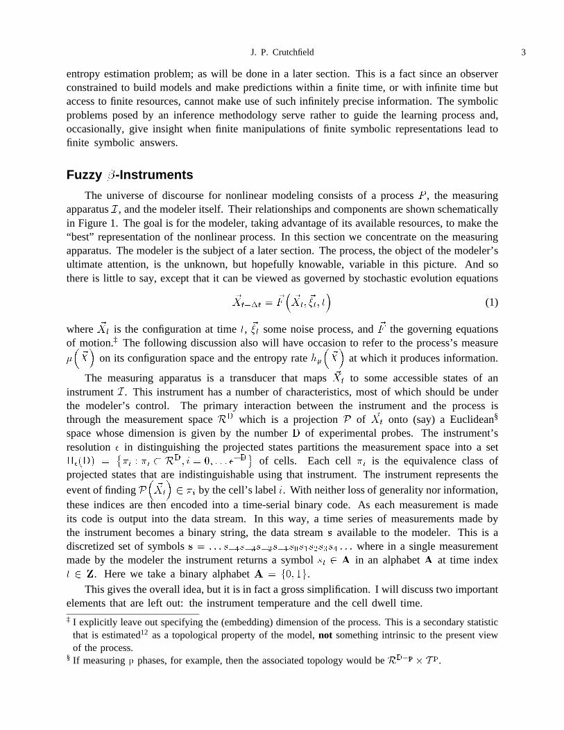
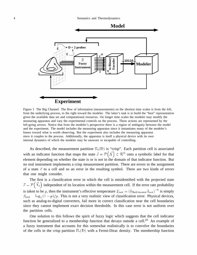
The universe of discourse for nonlinear modeling consists of a process� , the measuringapparatus�, and the modeler itself. Their relationships and components are shown schematicallyin Figure 1. The goal is for the modeler, taking advantage of its available resources, to make the“best” representation of the nonlinear process. In this section we concentrate on the measuringapparatus. The modeler is the subject of a later section. The process, the object of the modeler’sultimate attention, is the unknown, but hopefully knowable, variable in this picture. And sothere is little to say, except that it can be viewed as governed by stochastic evolution equations
������ � ������� ���� �
�(1)
where ��� is the configuration at time�, ��� some noise process, and�� the governing equationsof motion.‡ The following discussion also will have occasion to refer to the process’s measure�����
on its configuration space and the entropy rate�
����
at which it produces information.
The measuring apparatus is a transducer that maps��� to some accessible states of aninstrument�. This instrument has a number of characteristics, most of which should be underthe modeler’s control. The primary interaction between the instrument and the process isthrough the measurement space�� which is a projection� of ��� onto (say) a Euclidean§
space whose dimension is given by the number� of experimental probes. The instrument’sresolution in distinguishing the projected states partitions the measurement space into a set����� �
��� � �� � ��� � � �� � � � ��
�of cells. Each cell�� is the equivalence class of
projected states that are indistinguishable using that instrument. The instrument represents the
event of finding�����
�� �� by the cell’s label�. With neither loss of generality nor information,
these indices are then encoded into a time-serial binary code. As each measurement is madeits code is output into the data stream. In this way, a time series of measurements made bythe instrument becomes a binary string, the data stream� available to the modeler. This is adiscretized set of symbols� � � � �
�� �� �� �� � � � � � � � � where in a single measurementmade by the modeler the instrument returns a symbol � � � in an alphabet� at time index� � �. Here we take a binary alphabet� � ��� �.
This gives the overall idea, but it is in fact a gross simplification. I will discuss two importantelements that are left out: the instrument temperature and the cell dwell time.‡ I explicitly leave out specifying the (embedding) dimension of the process. This is a secondary statistic
that is estimated12 as a topological property of the model,not something intrinsic to the present viewof the process.
§ If measuring� phases, for example, then the associated topology would be���� � � �.
4 Semantics and Thermodynamics
...10110...Fuzzy
Instrument
to
Bin
ary
Enc
oder
D = 2 probesε
ε-D
ε-D
Modeler
Experiment
εβ
Model
1
Figure 1 The Big Channel. The flow of information (measurements) on the shortest time scales is from the left,from the underlying process, to the right toward the modeler. The latter’s task is to build the “best” representationgiven the available data set and computational resources. On longer time scales the modeler may modify themeasuring apparatus and vary the experimental controls on the process. These actions are represented by theleft-going arrows. Notice that from the modeler’s perspective there is a region of ambiguity between the modeland the experiment. The model includes the measuring apparatus since it instantiates many of the modeler’sbiases toward what is worth observing. But the experiment also includes the measuring apparatussince it couples to the process. Additionally, the apparatus is itself a physical device with its owninternal dynamics of which the modeler may be unaware or incapable of controlling.
As described, the measurement partition����� is “crisp”. Each partition cell is associated
with an indicator function that maps the state�� � ������ �� onto a symbolic label for that
element depending on whether the state is or is not in the domain of that indicator function. Butno real instrument implements a crisp measurement partition. There are errors in the assignmentof a state�� to a cell and so an error in the resulting symbol. There are two kinds of errorsthat one might consider.
The first is a classification error in which the cell is misidentified with the projected state�� � �
����
�independent of its location within the measurement cell. If the error rate probability
is taken to be�, then the instrument’s effective temperature����� � ����������������� is simply
����� � ��� �� ����. This is not a very realistic view of classification error. Physical devices,such as analog-to-digital converters, fail more in correct classification near the cell boundariessince they cannot implement exact decision thresholds. In this case error is not uniform overthe partition cells.
One solution to this follows the spirit of fuzzy logic which suggests that the cell indicatorfunction be generalized to a membership function that decays outside a cell.43 An example ofa fuzzy instrument that accounts for this somewhat realistically is to convolve the boundariesof the cells in the crisp partition����� with a Fermi-Dirac density. The membership function
J. P. Crutchfield 5
then becomes
������
�
�����
�
���������� ������������� � �(2)
where����� is the fuzzy partition’s inverse temperature and��� � �� is the cell’s center in the
measurement space. At zero temperature the crisp partition is recovered,��� ��� �
��������
At sufficiently high temperatures, the instrument outputs random sequences uncorrelated withthe process within the cell.
The algebra of fuzzy measurements will not be carried through the following. I will simplyleave behind at this point knowledge of the fuzzy partition. The particular consequences fordoing this correctly, though, will be reported elsewhere. The main result is that when donein this generality, the ensuing inference process is precluded from inferring too much and tooprecise a structure in the source.
The second element excluded from the Big Channel concerns the time��� spends in eachpartition cell. To account for this there should be an additional time series that gives the celldwell time for each state measurement. Only in special circumstances will the dwell time beconstant, if the partition is a uniform coarse-graining. When ergodicity can be appealed to theaverage dwell time� can be used. In any case, it is an important parameter and one that isreadily available, but often unused.
The dwell time suggests another instrument parameter, the frequency response; or, moreproperly dropping Fourier modeling bias, the instrument’s dynamic response. On short timescales the instrument’s preceding internal states can affect its resolution in determining thepresent state and the dwell time. In the simplest case, there is a shortest time below which theinstrument cannot respond. Then passages through a cell that are too brief will not be detectedor will be misreported.
All of these detailed instrumental properties can be usefully summarized by the informationacquisition rate ��. In its most general form it is given by the information gain of the fuzzypartition ��
� with respect to the process’s asymptotic distribution����
projected onto themeasurement space. That is,
���� � ��� � �������� �����
�������
(3)
where�� ��� is the information gain of distribution with respect to�. Assuming ignoranceof the process’s distribution allows some simplification and gives the measurement channelcapacity
���� � ��� � �������� ���
�
� ����� ��� �������� ���
�
where ����� ��� � ��� �� ������� � ���� �� � (4)
and where����� ���
�is the entropy of a cell’s membership function and������� is the
number of cells in the crisp partition. At high temperature����� ���
�����
��
������ ���
��� and
6 Semantics and Thermodynamics
the information acquisition rate vanishes, since each cell’s membership function widens to coverthe measurement space.
The Modeler
Beyond the instrument, one must consider what can and should be done with information inthe data stream. Acquisition of, processing, and inferring from the measurement sequence are thefunctions of the modeler. The modeler is essentially defined in terms of its available inferenceresources. These are dominated by storage capacity and computational power, but certainlyinclude the inference method’s efficacy, for example. Delineating these resources constitutes thebarest outline of an observer that builds models. Although the following discussion does notrequire further development at this abstract a level, it is useful to keep in mind since particularchoices for these elements will be presented.
The modeler is presented with�, the bit string, some properties of which were just given.The modeler’s concern is to go from it to a useful representation. To do this the modeler needs anotion of the process’s effective state and its effective equations of motion. Having built a modelrepresenting these two components, any residual error or deviation from the behavior describedby the model can be used to estimate the effective noise level of the process. It should be clearwhen said this way that the noise level and the sophistication of the model depend directly onthe data and on the modeler’s resources. Finally, the modeler may have access to experimentalcontrol parameters. And these can be used to aid in obtaining different data streams useful inimproving the model by (say) concentrating on behavior where the effective noise level is highest.
The central problem of nonlinear modeling now can be stated. Given an instrument, somenumber of measurements, and fixedfinite inference resources, how much computational structurein the underlying process can be extracted?
Limits to ModelingBefore pursuing this goal directly it will be helpful to point out several limitations imposed
by the data or the moder’s interpretation of it.
In describing the data stream’s character it was emphasized that the individual measurementsare only indirect representations of the process’s state. If the modeler interprets the measurementsas the process’s state, then it is unwittingly forced into a class of computationally less powerfulrepresentation. These consists of finite Markov chains with states in� or in some arbitrarilyselected state alphabet.|| This will become clearer through several examples used later on. It isimportant at this early stage to not over-interpret the measurements’ content as this might limitthe quality of the resulting models.
The instrument itself obviously constrains the observer’s ability to extract regularity fromthe data stream and so it directly affects the model’s utility. The most basic of these constraintsare given by Shannon’s coding theorems.40 The instrument was described as a transducer, but italso can be considered to be a communication channel between the process and the modeler. Thecapacity of this channel is�� � ����
���� ���
�. As � �� and if the process is deterministic
|| As done with hidden Markov models.18,37
J. P. Crutchfield 7
and has entropy������� �, a theorem of Kolmogorov’s says that this rate is maximized
for a given process if the crisp partition����� is generating.26 This property requires infinitesequences of cell indices to be in a finite-to-one correspondence with the process’s states. Asimilar result was shown to hold for the classes of process of interest here: deterministic, butcoupled to an extrinsic noise source.13 Note that the generating partition requirement necessarilydetermines the number� of probes required by the instrument.
For an instrument with a crisp generating partition, Shannon’s noiseless coding theorem saysthat the measurement channel must have a capacity higher than process’s entropy
�� � ��
����
(5)
If this is the case then the modeler can use the data stream to reconstruct a model of the processand, for example, estimate its entropy and complexity. These can be obtained to within errorlevels determined by the process’s extrinsic noise level.
If �� � ��
����
, then Shannon’s theorem for a channel with noise says that the modelerwill not be able to reconstruct a model with an effective noise level less than the equivocation
��
����� �� induced by the instrument. That is, there will be an “unreconstructable” portion of
the dynamics represented in the signal.
These results assume, as is also done implicitly in Shannon’s existence proofs for codes,that the modeler has access to arbitrary inference resources. When these are limited there willbe yet another corresponding loss in the quality of the model and an increase in the apparentnoise level. It is interesting to note that if one were to adopt Laplace’s philosophical stancethat all (classical) reality is deterministic and update it with the modern view that it is chaotic,then the instrumental limitations discussed here are the general case. And apparent randomnessis a consequence of them.
The Explanatory Channel
A clear statement of the observer’s goal is needed, beyond just estimating the best model.Surely a simple model is to be desired from the viewpoint of understandability of the process’smechanism and as far as implementation of the model in (say) a control system is concerned.Too simple a model, though, might miss important structure, rendering the process apparentlystochastic and highly unpredictable when it is deterministic, but nonlinear. The trade-off betweenmodel simplicity and large unpredictability can be explained in terms of a larger goal for themodeler: to explain to another observer the process’s behavior in the most concise manner,but in detail as well. Discussion of this interplay will be couched in terms of the explanatorychannel of Figure 2.
Before describing this view, it is best to start from some simple principles. To make contactwith existing approaches and for the brevity’s sake, the best model will be taken to be the mostlikely. If one had access to a complete probabilistic description of the modeling universe, thenthe goal would be to maximize the conditional probability������� of the model� given thedata stream�. This mythical complete probabilistic description���� �� is not available, but
8 Semantics and Thermodynamics
s = ...10110...Observer
AObserver
B
Explanation
X
Enc
oder
Simulator
s ObserverA
s’ = ...10110...
Model
M
Error Signal
E
Enc
oder
Simulators’
(a)
(b)
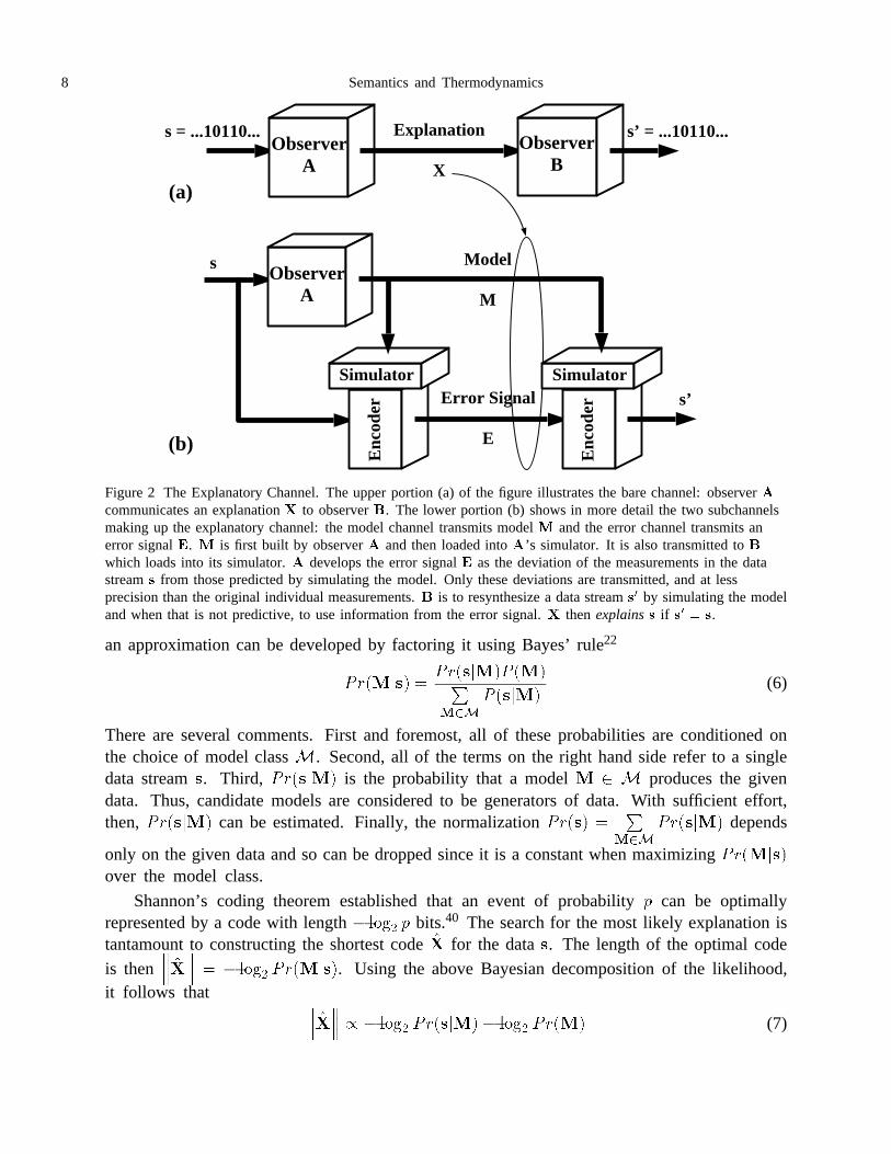
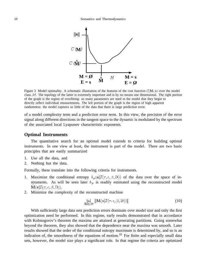
Figure 2 The Explanatory Channel. The upper portion (a) of the figure illustrates the bare channel: observer�
communicates an explanation� to observer�. The lower portion (b) shows in more detail the two subchannelsmaking up the explanatory channel: the model channel transmits model� and the error channel transmits anerror signal�. � is first built by observer� and then loaded into�’s simulator. It is also transmitted to�which loads into its simulator.� develops the error signal� as the deviation of the measurements in the datastream� from those predicted by simulating the model. Only these deviations are transmitted, and at lessprecision than the original individual measurements.� is to resynthesize a data stream�� by simulating the modeland when that is not predictive, to use information from the error signal.� thenexplains� if �� � �.
an approximation can be developed by factoring it using Bayes’ rule22
������� ��������� ����
���
� �����(6)
There are several comments. First and foremost, all of these probabilities are conditioned onthe choice of model class�. Second, all of the terms on the right hand side refer to a singledata stream�. Third, ������� is the probability that a model� � � produces the givendata. Thus, candidate models are considered to be generators of data. With sufficient effort,then,������� can be estimated. Finally, the normalization����� �
�
���
������� depends
only on the given data and so can be dropped since it is a constant when maximizing�������over the model class.
Shannon’s coding theorem established that an event of probability� can be optimallyrepresented by a code with length� ���
�� bits.40 The search for the most likely explanation is
tantamount to constructing the shortest code�� for the data�. The length of the optimal code
is then��� ����� � � ���
��������. Using the above Bayesian decomposition of the likelihood,
it follows that��� ����� � � ���� �������� ���� ����� (7)
J. P. Crutchfield 9
The resulting optimization procedure can be described in terms of the explanatory channel ofFigure 2. There are two observers� and� that communicate an explanation� via a channel.The input to this explanatory channel, what the modeler� sees, is the data stream�; the output,what� can resynthesize given the explanation� will be denoted��.
As shown in Figure 2(b)� is transmitted over two subchannels. The first is the modelingchannel along which a model� is communicated. The second is the error channel along whichan error signal� is transmitted.� is that portion of� unexplained by the model�.
There are two criteria for a good explanation:
1. � must explain�. That is,� must be able to resynthesize the original data:�� � �.
2. The explanation must be as short as possible. That is, the length��� � ��� � ��� inbits of � must be minimized.
The efficiency of an explanation or, equivalently, of the model is measured by the compressionratio
���� �� ����
�������� ���
���(8)
This quantifies the efficacy of an explanation employing model�. � is then a cost functionover the space� of possible models. The optimal model�� then minimizes this cost
����� �
�� ������
���� �� (9)
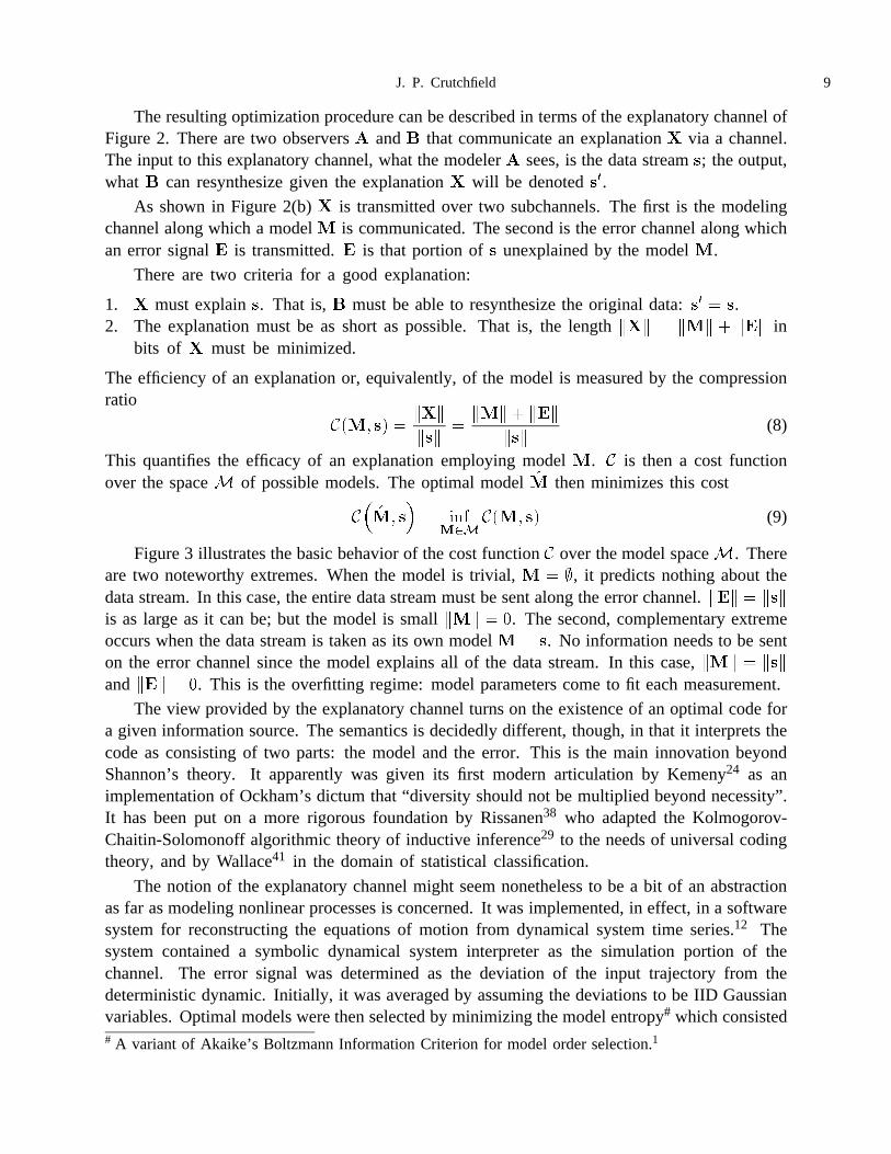
Figure 3 illustrates the basic behavior of the cost function� over the model space�. Thereare two noteworthy extremes. When the model is trivial,� � �, it predicts nothing about thedata stream. In this case, the entire data stream must be sent along the error channel.��� � ���is as large as it can be; but the model is small��� � . The second, complementary extremeoccurs when the data stream is taken as its own model� � �. No information needs to be senton the error channel since the model explains all of the data stream. In this case,��� � ���and��� � . This is the overfitting regime: model parameters come to fit each measurement.
The view provided by the explanatory channel turns on the existence of an optimal code fora given information source. The semantics is decidedly different, though, in that it interprets thecode as consisting of two parts: the model and the error. This is the main innovation beyondShannon’s theory. It apparently was given its first modern articulation by Kemeny24 as animplementation of Ockham’s dictum that “diversity should not be multiplied beyond necessity”.It has been put on a more rigorous foundation by Rissanen38 who adapted the Kolmogorov-Chaitin-Solomonoff algorithmic theory of inductive inference29 to the needs of universal codingtheory, and by Wallace41 in the domain of statistical classification.
The notion of the explanatory channel might seem nonetheless to be a bit of an abstractionas far as modeling nonlinear processes is concerned. It was implemented, in effect, in a softwaresystem for reconstructing the equations of motion from dynamical system time series.12 Thesystem contained a symbolic dynamical system interpreter as the simulation portion of thechannel. The error signal was determined as the deviation of the input trajectory from thedeterministic dynamic. Initially, it was averaged by assuming the deviations to be IID Gaussianvariables. Optimal models were then selected by minimizing the model entropy# which consisted# A variant of Akaike’s Boltzmann Information Criterion for model order selection.1
10 Semantics and Thermodynamics
||s||
M
MC( )
M = s E = O
M = OE = s M
MC( )
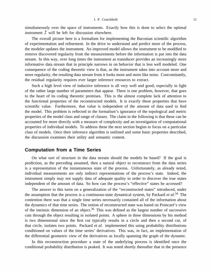
Figure 3 Model optimality. A schematic illustration of the features of the cost function���� �� over the modelclass�. The topology of the latter is extremely important and is by no means one dimensional. The right portionof the graph is the region of overfitting: so many parameters are used in the model that they begin todirectly reflect individual measurements. The left portion of the graph is the region of high apparentrandomness: the model captures so little of the data that there is large prediction error.
of a model complexity term and a prediction error term. In this view, the precision of the errorsignal along different directions in the tangent space to the dynamic is modulated by the spectrumof the associated local Lyapunov characteristic exponents.
Optimal InstrumentsThe quantitative search for an optimal model extends to criteria for building optimal
instruments. In one view at least, the instrument is part of the model. There are two basicprinciples that are easily summarized
1. Use all the data, and2. Nothing but the data.
Formally, these translate into the following criteria for instruments.
1. Maximize the conditional entropy��������� �� ����� of the data over the space of in-struments. As will be seen later�� is readily estimated using the reconstructed model��������� �� �����.
2. Minimize the complexity of the reconstructed machine
������
��������� �� ������ (10)
With sufficiently large data sets prediction errors dominate over model size and only the firstoptimization need be performed. In this regime, early results demonstrated that in accordancewith Kolmogorov’s theorem the maxima are attained at generating partitions. Going somewhatbeyond the theorem, they also showed that the dependence near the maxima was smooth. Laterresults showed that the order of the conditional entropy maximum is determined by, and so is anindication of, the smoothness of the equations of motion.10 For finite and especially small datasets, however, the model size plays a significant role. In that regime the criteria are optimized
J. P. Crutchfield 11
simultaneously over the space of instruments. Exactly how this is done to select the optimalinstrument�� will be left for discussion elsewhere.
The overall picture here is a formalism for implementing the Baconian scientific algorithmof experimentation and refinement. In the drive to understand and predict more of the process,the modeler updates the instrument. An improved model allows the instrument to be modified toremove discovered regularity from the measurements before the information is put into the datastream. In this way, over long times the instrument as transducer provides an increasingly moreinformative data stream that in principle narrows in on behavior that is less well modeled. Oneconsequence of the coding theoretic view is that, as the instrument takes into account more andmore regularity, the resulting data stream from it looks more and more like noise. Concomitantly,the residual regularity requires ever larger inference resources to extract.
Such a high level view of inductive inference is all very well and good; especially in lightof the rather large number of parameters that appear. There is one problem, however, that goesto the heart of its coding theoretic premises. This is the almost complete lack of attention tothe functional properties of the reconstructed models. It is exactly these properties that havescientific value. Furthermore, that value is independent of the amount of data used to findthe model. This problem is reflected in the formalism’s ignorance of the topological and metricproperties of the model class and range of classes. The claim in the following is that these can beaccounted for more directly with a measure of complexity and an investigation of computationalproperties of individual models. To address these the next section begins to focus on a particularclass of models. Once their inference algorithm is outlined and some basic properties described,the discussion examines their utility and semantic content.
Computation from a Time Series
On what sort of structure in the data stream should the models be based? If the goal isprediction, as the preceding assumed, then a natural object to reconstruct from the data seriesis a representation of the instantaneous state of the process. Unfortunately, as already noted,individual measurements are only indirect representations of the process’s state. Indeed, theinstrument simply may not supply data of adequate quality in order to discover the true statesindependent of the amount of data. So how can the process’s “effective” states be accessed?
The answer to this turns on a generalization of the “reconstructed states” introduced, underthe assumption that the process is a continuous-state dynamical system, by Packardet al.34 Thecontention there was that a single time series necessarily contained all of the information aboutthe dynamics of that time series. The notion of reconstructed state was based on Poincar´e’s viewof the intrinsic dimension of an object.36 This was defined as the largest number of successivecuts through the object resulting in isolated points. A sphere in three dimensions by his methodis two dimensional since the first cut typically results in a circle and then a second cut, ofthat circle, isolates two points. Packardet al. implemented this using probability distributionsconditioned on values of the time series’ derivatives. This was, in fact, an implementation ofthe differential geometric view of the derivatives as locally spanning the graph of the dynamic.
In this reconstruction procedure a state of the underlying process is identified once theconditional probability distribution is peaked. It was noted shortly thereafter that in the presence
12 Semantics and Thermodynamics
of extrinsic noise a number of conditions is reached beyond which the conditional distributionis no longer sharpened.13 And, as a result the process’s state cannot be further identified. Thewidth of the resulting distribution then gives an estimate of the effective extrinsic noise leveland the minimum number of conditions first leading to this situation, an estimate of the effectivedimension.
The method of time derivative reconstruction gives the key to discovering states in discretetimes series.* For discrete time series a state is defined to be the set of subsequences thatrender the future conditionally independent of the past.14† Thus, the observer identifies a stateat different times in the data stream as its being in identical conditions of ignorance about thefuture. The set of future subsequences following from a state is called itsmorph.
For this definition of state several reconstruction procedures have been developed. In brief,the simplest method consists of three steps. In the first all length� subsequences in the datastream are represented as paths in a depth� binary “parse” tree. In the second, the morphs arediscovered by associating them with the distinct depth� � ��� subtrees found in the parse treedown to depth���. The number of morphs is then the number of effective states. In the finalstep, the state to state transitions are found by looking at how each state’s associated subtreesmap into one another on the parse tree.11,14,15
This procedure reconstructs from a data stream a “topological” machine: the skeleton ofstates and allowed transitions. There are a number of issues concerning statistical estimation,including error analysis and probabilistic structure, that need to be addressed.16 But this outlinesuffices for the present purposes. The estimated models are referred to as�-machines in orderto indicate their dependence not only on measurement resolution, but also indirectly on all ofthe instrumental and inferential parameters discussed so far.
�-Machines
The product of machine reconstruction is a set of states that will be associatedwith a set � � ��� of vertices and a set of transitions associated with a set� ��� � � � ��
�
��� �� �� � �� � � ��
of labeled edges. Formally, the reconstruction proce-
dure puts no limit on the number of machine states inferred. Indeed, in some important casesthe number is infinite, such as at phase transitions.15 In the following� will be a finite setand the machines “finitary”. One depiction of the reconstructed machine is as a labeleddirected graph � �����. Examples will be seen shortly. The full probabilistic structure isdescribed by a set of transition matrices
� �
�� ���
�
�� ���
���
�
� ���
�
��� �� �� � �� � � �
�(11)
where ����
�� denotes the conditional probability to make a transition to state�
� from state�
on observing symbol�.
* The time delay method appears not to generalize.† This notion of state is widespread; appearing in various guises in early symbolic dynamics, ergodic,
and automata theories. It is the basic notion of state in Markov chain theory.
J. P. Crutchfield 13
A stochastic machine is a compact way of describing the probabilities of a possiblyinfinite number of measurement sequences. The probability of a given sequence�
� ������� � � � ����� �� � �� is recovered from the machine by the telescoping product of condi-tional transition probabilities
�����
� ���������
��������
�� � � � ����� �
����
�� (12)
Here�� is the unique start state. It is the state of total ignorance, so that at the first time stepwe take��� � �. The sequence��� ��� ��� � � � � ����� �� consists of those states through whichthe sequence drives the machine. To summarize, a machine is the set� � �������� � ���.
Several important statistical properties are captured by the stochastic connection matrix
� �����
� ��� (13)
where�� ���� � ����� is the state to state transition probability, unconditioned by the measure-ment symbols. By construction every state has an outgoing transition. This is reflected in thefact that� is a stochastic matrix:
�����
���� � �. It should be clear that by dropping the input
alphabet transition labels from the machine the detailed, call it “computational”, structure of theinput data stream has been lost. All that is retained in� is the state transition structure and thisis a Markov chain. The interesting fact is that Markov chains are a proper subset of stochasticfinitary machines. Examples later on will support this contention. It is at exactly this step ofunlabeling the machine that the “properness” appears.
The stationary state probabilities��� �
��� �
����
�� � �� � � �
�are given by the left
eigenvector of�
���� � ��� (14)
The entropy rate of the Markov chain is then
���� � � �����
�������
����� ��� ����� (15)
This measures the information production rate in bits per time step of the Markov chain. Althoughthe mapping from input strings to the chain’s transition sequences is not in general one-to-one,it is finite-to-one. And so, the Markov chain entropy rate is also the entropy rate of the originaldata source
����� � �����
�������
����
����
�� ��� ����
�� (16)
The complexity‡ quantifies the information in the state-alphabet sequences
���� � ����� � �����
�� ��� �� (17)
‡ Within the reconstruction hierarchy this is actually the finitary complexity, since the context of thediscussion implies that we are considering processes with a finite amount of memory. However, I havenot introduced this restriction in unnecessary places in the discussion. The finitary complexity has beenconsidered before in the context of generating partitions and known equations of motion.19,31,42
14 Semantics and Thermodynamics
It measures the amount of memory in the process. For completeness, note that there is anedge-complexity that is the information contained in the asymptotic edge distribution��� ���� � �����
�
�� � �� �� � �� � � �� � � �
�
��
��� � � �
����
�� ���� �� (18)
These quantities are not independent. Conservation of information at each state leads to therelation
��
�� �� � � (19)
And so, there are only two independent quantities when modeling a process as a stochasticfinitary machine. The entropy�, as a measure of the diversity of patterns, and the complexity��, as a measure of memory, have been taken as the two elementary coordinates with whichto analyze a range of sources.15
There is another set of quantities that derive from the skeletal structure of the machine.Dropping all of probabilistic structure, the growth rate of the number of sequences it producesis the topological entropy
� �������� (20)
where� is the principle eigenvalue of the connection matrix�� �����
����� . The latter is
formed from the labeled matrices��
���� �
��
����
����
�
� ���
�
�� �
��� ���� � � �
�(21)
The state and transition topological complexities are
� � ���� ���
�� � ���� ���(22)
In computation theory, an object’s complexity is generally taken to be the size in bitsof its representation. The quantities just defined measure the complexity of the reconstructedmachine. As will be seen in the penultimate section, when these entropies and complexities, bothtopological and metric, are integrated into a single parametrized framework, a thermodynamicsof machines emerges.
Complexity
It is useful at this stage to stop and reflect on some properties of the models that we have justdescribed how to reconstruct. Consider two extreme data sources. The first, highly predictable,produces a streams of 1s; the second, highly unpredictable, is an ideal random source of a binarysymbols. The parse tree of the predictable source is a single path of 1s. And there is a singlesubtree, at any depth. As a result the machine has a single state and a single transition on� � :a simple model of a simple source. For the ideal random source the parse tree, again to any
J. P. Crutchfield 15
depth, is the full binary tree. All paths appear in the parse tree since all binary subsequencesare produced by the source. There is a single subtree, of any morph depth at all parse treedepths: the full binary subtree. And the machine has a single state with two transitions; oneon � � � and one on� � �. A simple machine, even though the source produces the widestdiversity of binary sequences.
A simple gedanken experiment serves to illustrate how complexity is a measure of amachine’s memory capacity. Consider two observers� and�, each with the same model� of some process.� is allowed to start machine� in any state and uses it to generatebinary strings that are determined by the edge labels of the transitions taken. These stringsare passed to observer� which traces there effect through its own copy of�. On averagehow much information about�’s state can� communicate to� via the binary strings? Ifthe machine describes (say) a period three process, e.g. it outputs strings like��������� � � �,��������� � � �, and ��������� � � �, it has ��� � � states. Since� starts� in differentstates,� can learn only the information of the process’s phase in the period 3 cycle. Thisis ���
���� � ��� � � � bits of information about the process’s state, if� chooses the initial
states with equal probability. However, if the machine describes an idea random binary process,by definition� can communicate no information to�, since there is no structure in the sequencesto use for this purpose. This is reflected in the fact, as already noted above, that the correspondingmachine has a single state and its complexity is���
�� � �. In this way, a process’s complexity
is the amount of information that someone controlling its start state can communicate to another.
These examples serve to highlight one of the most basic properties of complexity, as I usethe term. Both predictable and random sources are simple in the sense that their models aresmall. Complex processes in this view have large models. In computational terms, complexprocesses have, as a minimum requirement, a large amount of memory as revealed by manyinternal states in the reconstructed machine. Most importantly, that memory is structured inparticular ways that support different types of computation. The sections below on knowledgeand meaning show several consequences of computational structure.
In the most general setting, I use the word “complexity” to refer to the amount of informationcontained in observer-resolvable equivalence classes. For finitary machines, the complexity ismeasured by the quantities labeled above by�. This notion has been referred to as the “statisticalcomplexity” in order to distinguish it from the Chaitin-Kolmogorov complexity,9,27 the Lempel-Ziv complexity,28 Rissanen’s stochastic complexity,38 and others45,44 which are all equivalent
in the limit of long data streams to the process’s Kolmogorov-Sinai entropy��
����
. If the
instrument is generating and�����
is absolutely continuous, these quantities are given by the
entropy rate of the reconstructed machine, Eq. (16).7 Accordingly, I use the word “entropy” torefer to such quantities. They measure the diversity of sequences a process produces. Implicitin their definitions is the restriction that the modeler must pay computationally for each randombit. Simply stated, the overarching goal is exact description of the data stream. In the modelingapproach advocated here the modeler is allowed to flip a coin or to sample the heat bath to whichit may be coupled. “Complexity” is reserved in my vocabulary to refer to a process’s structuralproperties, such as memory and other types of computational capacity.
16 Semantics and Thermodynamics
This is not the place to review the wide range of alternative notions of “complexity” thathave been discussed more recently in the physics and dynamics literature. The reader is referredto the comments and especially the citations elsewhere.14,15 It is important to point out, however,that the notion defined here does not require knowledge of the equations of motion, the priorexistence of exact conditional probabilities, Markov or even generating partitions of the statespace, continuity and differentiability of the state variables, nor the existence of periodic orbits.Furthermore, the approach taken here differs from those based on the construction of universalcodes in the emphasis on the model’s structure. That emphasis brings it into direct contact withthe disciplines of stochastic automata, formal language theory, and thermodynamics.
Finally, statistical complexity is a highly relative concept that depends directly on theassumed model class. In the larger setting of hierarchical reconstruction it becomes the finitarycomplexity since it measures the number of states in a finite state machine representation. Butthere are other versions appropriate, for example, when the finitary complexity diverges.11
Causality
There are a few points that must be brought out concerning what these reconstructed machinesrepresent. First, by the definition of future-equivalent states, the machines give the minimalinformation dependency between the morphs. In this respect, they represent the causality of themorphs considered as events. The machines capture the information flow within the given datastream. If state B follows state A then A is a cause of B and B is one effect of A. Second, machinereconstruction produces minimal models up to the given prediction error level. This minimalityguarantees that there are no other events (morphs) that intervene, at the given error level, torender A and B independent. In this case, we say that information flows from A to B. Theamount of information that flows is the negative logarithm of the connecting edge probability.Finally, time is the natural ordering captured by machines. An�-machine for a process is thenthe minimal causal representation reconstructed using the least powerful computational modelclass that yields a finite complexity.
KNOWLEDGE RELAXATION
The next two sections investigate how models can be used by an observer. An observer’sknowledge�� of a process� consists of the data stream, its current model, and how theinformation used to build the model was obtained.* Here the latter is given by the measuringinstrument� �
���� ���� �
�. To facilitate interpretation and calculations, the following will
assume a simple data acquisition discipline with uniform sampling interval� and a time-independent zero temperature measurement partition��. Further simplification comes fromignoring external factors, such as what the observer intends or needs to do with the model, byassuming that the observer’s goal is solely optimal prediction with respect to the model classof finitary machines.
* In principle, the observer’s knowledge also consists of the reconstruction method and its variousassumptions. But it is best to not elaborate this here. These and other unmentioned variables areassumed to be fixed.
J. P. Crutchfield 17
The totality of knowledge available to an observer is given by the development of its��
at each moment during its history. If we make the further assumption that by some agencythe observer has at each moment in its history optimally encoded the available current and pastmeasurements into its model, then the totality of knowledge consists of four parts: the timeseries of measurements, the instrument by which they were obtained, and the current modeland its current state. Stating these points so explicitly helps to make clear the upper bound onwhat the observer can know about its environment. Even if the observer is allowed arbitrarycomputational resources, given either finite information from a process or finite time, only afinite amount of structure can be inferred.
An �-machine is a representations of an observer’s model of a process. To see its role in thechange in�� consider the situation in which the model structure is kept fixed. Starting fromthe state�� of total ignorance about the process’s state, successive steps through the machinelead to a refinement of the observer’s knowledge as determined by a sequence of measurements.The average increase in�� is given by a diffusion of information throughout the model. Themachine transition probabilities, especially those connected with transient states, govern how theobserver gains more information about the process with longer measurement sequences.
A measure of information relaxation on finitary machines is given by the time-dependentfinitary complexity
����� � ��������� (23)
where��� � ��
����
�� ���� �� is the Shannon entropy of the distribution� � ���� and
������ �� � ������ (24)
is the probability distribution at time� beginning with the initial distribution���� � �� �
concentrated on the start state. This distribution represents the observer’s state of total ignoranceof the process’s state, i.e. before any measurements have been made, and correspondingly���� � . ����� is simply (the negative of) the Boltzmann�-function in the present setting.And we have the analogous result to the�-theorem for stochastic�-machines:����� convergesmonotonically when������ is sufficiently close to��� � ������: ����� �
�����. That is, the
time-dependent complexity limits on the finitary complexity. Furthermore, the observer has themaximal amount of information about the process, i.e. the observer’s knowledge is in equilibriumwith the process, when����� �� � ����� vanishes for all� � �����, where����� is some fixedtime characteristic of the process.
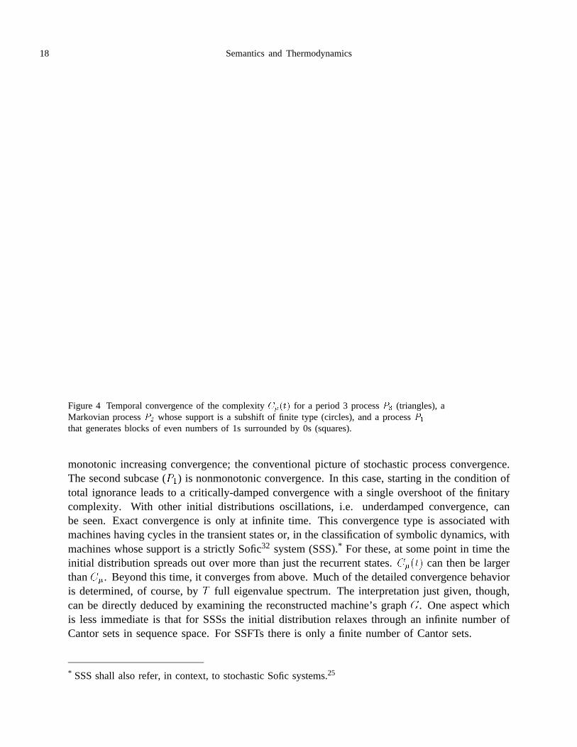
For finitary machines there are two convergence behaviors for�����. These are illustratedin figure 4 for three processes: one�� which is period 3 and generates�����, one�� in whichonly isolated zeros are allowed, and one�� that generates 1s in blocks of even length boundedby 0s. The first behavior type, illustrated by�� and��, is monotonic convergence from below.In fact, the asymptotic approach occurs in finite time. This is the case for periodic and recurrentMarkov chains, where the latter refers to finite state stochastic processes whose support is asubshift of finite type (SSFT). The convergence here is over-damped.
The second convergence type, illustrated by��, is only asymptotic; convergence to theasymptotic state distribution is only at infinite time. There are two subcases. The first is
18 Semantics and Thermodynamics
Figure 4 Temporal convergence of the complexity����� for a period 3 process�� (triangles), aMarkovian process�� whose support is a subshift of finite type (circles), and a process��
that generates blocks of even numbers of 1s surrounded by 0s (squares).
monotonic increasing convergence; the conventional picture of stochastic process convergence.The second subcase (��) is nonmonotonic convergence. In this case, starting in the condition oftotal ignorance leads to a critically-damped convergence with a single overshoot of the finitarycomplexity. With other initial distributions oscillations, i.e. underdamped convergence, canbe seen. Exact convergence is only at infinite time. This convergence type is associated withmachines having cycles in the transient states or, in the classification of symbolic dynamics, withmachines whose support is a strictly Sofic32 system (SSS).* For these, at some point in time theinitial distribution spreads out over more than just the recurrent states.����� can then be largerthan��. Beyond this time, it converges from above. Much of the detailed convergence behavioris determined, of course, by� full eigenvalue spectrum. The interpretation just given, though,can be directly deduced by examining the reconstructed machine’s graph�. One aspect whichis less immediate is that for SSSs the initial distribution relaxes through an infinite number ofCantor sets in sequence space. For SSFTs there is only a finite number of Cantor sets.
* SSS shall also refer, in context, to stochastic Sofic systems.25
J. P. Crutchfield 19
This structural analysis indicates that the ratio
������ ��� � �����
��(25)
is largely determined by the amount of information in the transient states. For SSSs this quantityonly asymptotically vanishes since there are transient cycles in which information persists for alltime, even though their probability decreases asymptotically. This leads to general definition of(chaotic or periodic) phase and phase locking. The phase of a machine at some point in time is itscurrent state. There are two types of phase of interest here. The first is the process’s phase and thesecond is the observer’s phase which refers to the state of the observer’s model having read thedata stream up to some time. The observer has�-locked onto the process when���������� � �.This occurs at the locking time����� which is the longest time� such that������ � �. Whenthe process is periodic, this notion of locking is the standard one from engineering. But it alsoapplies to chaotic processes and corresponds to the observer knowing what state the process isin, even if the next measurement cannot be predicted exactly.
These two classes of knowledge relaxation lead to quite different consequences for anobserver even though the processes considered above all have a small number of states (2or 3) and share the same single-symbol statistics:���� � �� � �
�and���� � �� � �
�. In the
over-damped case, the observer knows the state of the underlying process with certainty aftera finite time. In the critically-damped situation, however, the observer has only approximateknowledge for all times. For example, setting� � �� leads to locking times shown in table 1.Thus, the ability of an observer to infer the state depends crucially on the process’s computationalstructure, viz. whether its topological machine is a SSFT or a SSS. The presence of extrinsicnoise and observational noise modify these conclusions systematically.
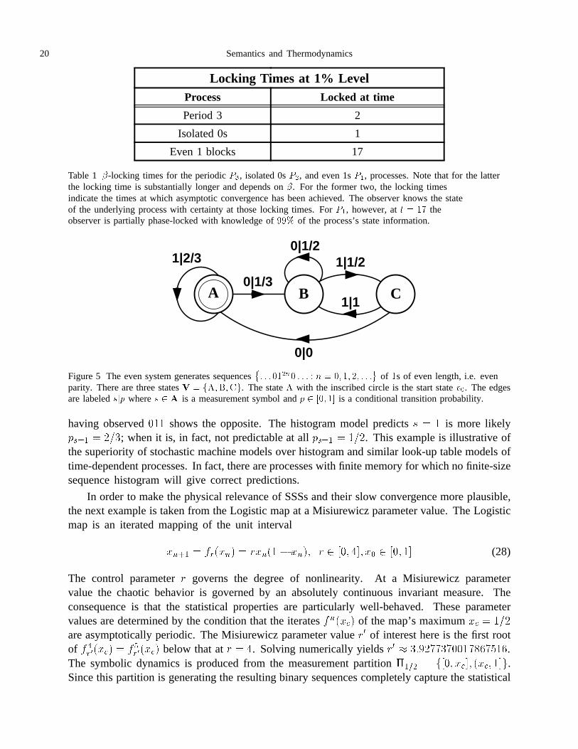
It is worthwhile to contrast the machine model of�� with a model based on histograms,or look-up tables, of the same process. Both models are given sufficient storage to exactlyrepresent the length 3 sequence probability distribution. They are then used for predictions onlength 4 sequences. The histogram model will store the probabilities for each length 3 sequence.This requires 8 bins each containing an 8 bit approximation of a rational number: 3 bits for thenumerator and 5 for the denominator. The total is 67 bits which includes an indicator for themost recent length 3 sequence. The machine model, see Figure 5, must store the current stateand five approximate rational numbers, the transition probabilities, using 3 bits each: one forthe numerator and two for the denominator. This gives a model size of 17 bits.
Two observers, each given one or the other model, are presented with the sequence���.What do they predict for the event that the fourth symbol is� � �? The histogram model predicts
��������� � �������� ��������
�������
���
��
�
�(26)
whereas the machine model predicts
��������� � ��� � � (27)
The histogram model gives the wrong prediction. It says that the fourth symbol is uncertainwhen it is completely predictable. A similar analysis for the prediction of measuring� � �
20 Semantics and Thermodynamics
Locking Times at 1% LevelProcess Locked at time
Period 3 2
Isolated 0s 1
Even 1 blocks 17
Table 1 �-locking times for the periodic��, isolated 0s��, and even 1s��, processes. Note that for the latterthe locking time is substantially longer and depends on�. For the former two, the locking timesindicate the times at which asymptotic convergence has been achieved. The observer knows the stateof the underlying process with certainty at those locking times. For��, however, at� � �� theobserver is partially phase-locked with knowledge of��� of the process’s state information.
B CA
1|2/3
0|1/31|1/2
0|1/2
1|1
0|0
Figure 5 The even system generates sequences�� � � ����� � � � � � � �� ��� � � �
�of �s of even length, i.e. even
parity. There are three states� � ������. The state with the inscribed circle is the start state��. The edgesare labeled��� where� � � is a measurement symbol and� � �� �� is a conditional transition probability.
having observed��� shows the opposite. The histogram model predicts� � � is more likely���� � ���; when it is, in fact, not predictable at all�
��� � ���. This example is illustrative ofthe superiority of stochastic machine models over histogram and similar look-up table models oftime-dependent processes. In fact, there are processes with finite memory for which no finite-sizesequence histogram will give correct predictions.
In order to make the physical relevance of SSSs and their slow convergence more plausible,the next example is taken from the Logistic map at a Misiurewicz parameter value. The Logisticmap is an iterated mapping of the unit interval
���� � �
���
�� � ��
���� �
��� � � ��� ��� � ��� �� (28)
The control parameter� governs the degree of nonlinearity. At a Misiurewicz parametervalue the chaotic behavior is governed by an absolutely continuous invariant measure. Theconsequence is that the statistical properties are particularly well-behaved. These parametervalues are determined by the condition that the iterates������ of the map’s maximum�� � ���are asymptotically periodic. The Misiurewicz parameter value�� of interest here is the first rootof � �
������ � ��
������ below that at� � . Solving numerically yields�� � ���������� �����.The symbolic dynamics is produced from the measurement partition���� � ���� ���� ���� ���.Since this partition is generating the resulting binary sequences completely capture the statistical
J. P. Crutchfield 21
0|0.2760|0.364
1|0.724
1|0.636
D
1|1.000
1|0.479BA
0|0.521
C
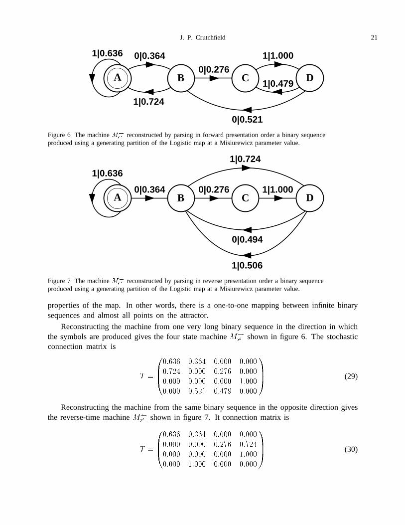
Figure 6 The machine���� reconstructed by parsing in forward presentation order a binary sequence
produced using a generating partition of the Logistic map at a Misiurewicz parameter value.
0|0.2760|0.364
1|0.636
D1|1.000
1|0.506
BA
0|0.494
C
1|0.724
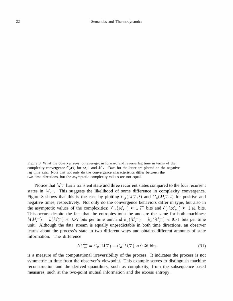
Figure 7 The machine���� reconstructed by parsing in reverse presentation order a binary sequence
produced using a generating partition of the Logistic map at a Misiurewicz parameter value.
properties of the map. In other words, there is a one-to-one mapping between infinite binarysequences and almost all points on the attractor.
Reconstructing the machine from one very long binary sequence in the direction in whichthe symbols are produced gives the four state machine�
�
�� shown in figure 6. The stochastic
connection matrix is
� �
��������� ����� ����� �����
����� ����� ����� �����
����� ����� ����� �����
����� ���� ���� �����
���� (29)
Reconstructing the machine from the same binary sequence in the opposite direction givesthe reverse-time machine��
�� shown in figure 7. It connection matrix is
� �
��������� ����� ����� �����
����� ����� ����� �����
����� ����� ����� �����
����� ����� ����� �����
���� (30)
22 Semantics and Thermodynamics
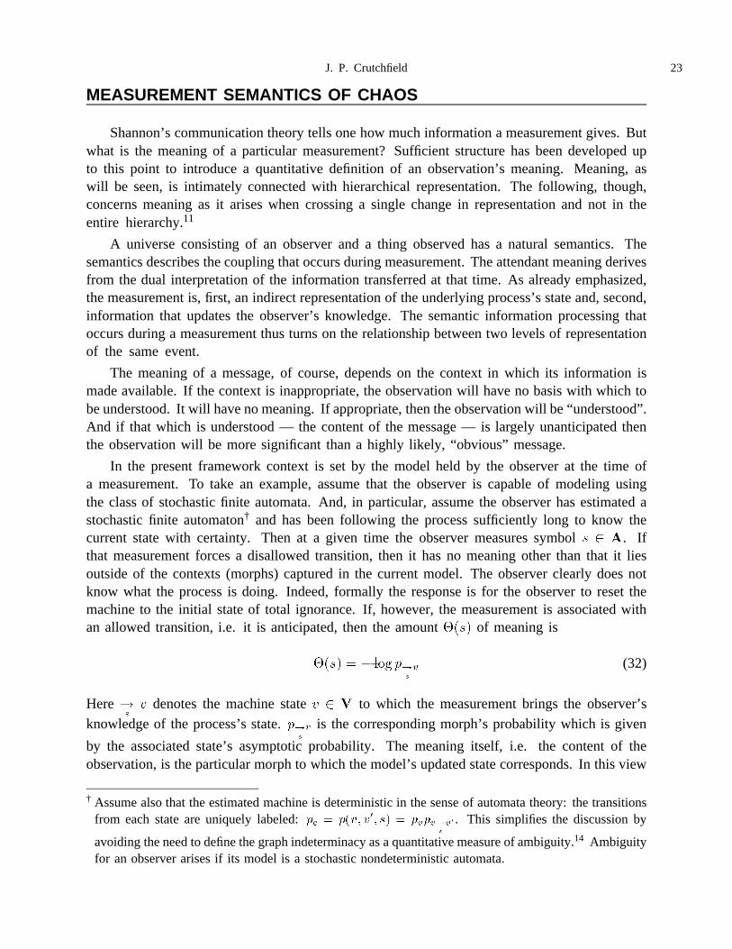
Figure 8 What the observer sees, on average, in forward and reverse lag time in terms of thecomplexity convergence����� for ��
�� and���� . Data for the latter are plotted on the negative
lag time axis. Note that not only do the convergence characteristics differ between thetwo time directions, but the asymptotic complexity values are not equal.
Notice that���
� has a transient state and three recurrent states compared to the four recurrentstates in��
�� . This suggests the likelihood of some difference in complexity convergence.
Figure 8 shows that this is the case by plotting�����
�� � �� and�����
�� � �� for positive andnegative times, respectively. Not only do the convergence behaviors differ in type, but also inthe asymptotic values of the complexities:����
�
�� � � ���� bits and�����
�� � � ���� bits.This occurs despite the fact that the entropies must be and are the same for both machines:����
�� � � ������ � � ��� bits per time unit and������� � � ����
�
�� � � ���� bits per timeunit. Although the data stream is equally unpredictable in both time directions, an observerlearns about the process’s state in two different ways and obtains different amounts of stateinformation. The difference
���
� �����
�� �� �����
�� � � ���� bits (31)
is a measure of the computational irreversibility of the process. It indicates the process is notsymmetric in time from the observer’s viewpoint. This example serves to distinguish machinereconstruction and the derived quantifiers, such as complexity, from the subsequence-basedmeasures, such at the two-point mutual information and the excess entropy.
J. P. Crutchfield 23
MEASUREMENT SEMANTICS OF CHAOS
Shannon’s communication theory tells one how much information a measurement gives. Butwhat is the meaning of a particular measurement? Sufficient structure has been developed upto this point to introduce a quantitative definition of an observation’s meaning. Meaning, aswill be seen, is intimately connected with hierarchical representation. The following, though,concerns meaning as it arises when crossing a single change in representation and not in theentire hierarchy.11
A universe consisting of an observer and a thing observed has a natural semantics. Thesemantics describes the coupling that occurs during measurement. The attendant meaning derivesfrom the dual interpretation of the information transferred at that time. As already emphasized,the measurement is, first, an indirect representation of the underlying process’s state and, second,information that updates the observer’s knowledge. The semantic information processing thatoccurs during a measurement thus turns on the relationship between two levels of representationof the same event.
The meaning of a message, of course, depends on the context in which its information ismade available. If the context is inappropriate, the observation will have no basis with which tobe understood. It will have no meaning. If appropriate, then the observation will be “understood”.And if that which is understood — the content of the message — is largely unanticipated thenthe observation will be more significant than a highly likely, “obvious” message.
In the present framework context is set by the model held by the observer at the time ofa measurement. To take an example, assume that the observer is capable of modeling usingthe class of stochastic finite automata. And, in particular, assume the observer has estimated astochastic finite automaton† and has been following the process sufficiently long to know thecurrent state with certainty. Then at a given time the observer measures symbol� � �. Ifthat measurement forces a disallowed transition, then it has no meaning other than that it liesoutside of the contexts (morphs) captured in the current model. The observer clearly does notknow what the process is doing. Indeed, formally the response is for the observer to reset themachine to the initial state of total ignorance. If, however, the measurement is associated withan allowed transition, i.e. it is anticipated, then the amount���� of meaning is
���� � � ��� ��
�
�(32)
Here��
� denotes the machine state� � � to which the measurement brings the observer’s
knowledge of the process’s state.��
�
� is the corresponding morph’s probability which is given
by the associated state’s asymptotic probability. The meaning itself, i.e. the content of theobservation, is the particular morph to which the model’s updated state corresponds. In this view
† Assume also that the estimated machine is deterministic in the sense of automata theory: the transitionsfrom each state are uniquely labeled:�� � ���� ��� �� � �����
�
�� . This simplifies the discussion by
avoiding the need to define the graph indeterminacy as a quantitative measure of ambiguity.14 Ambiguityfor an observer arises if its model is a stochastic nondeterministic automata.
24 Semantics and Thermodynamics
a measurement selects a particular pattern from a palette of morphs. The measurement’s meaningis the selected morph‡ and the amount of meaning is determined by the latter’s probability.
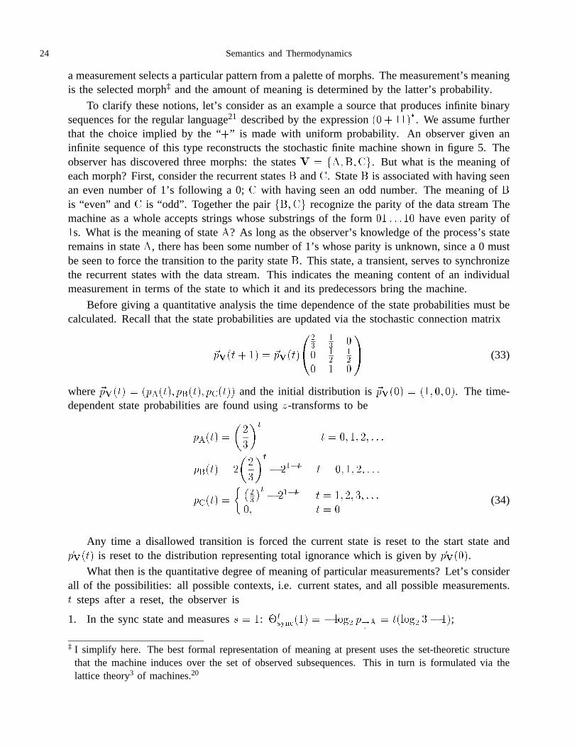
To clarify these notions, let’s consider as an example a source that produces infinite binarysequences for the regular language21 described by the expression�� � ����. We assume furtherthat the choice implied by the “�” is made with uniform probability. An observer given aninfinite sequence of this type reconstructs the stochastic finite machine shown in figure 5. Theobserver has discovered three morphs: the states� � ������. But what is the meaning ofeach morph? First, consider the recurrent states� and. State� is associated with having seenan even number of 1’s following a 0; with having seen an odd number. The meaning of�
is “even” and is “odd”. Together the pair���� recognize the parity of the data stream Themachine as a whole accepts strings whose substrings of the form�� �� have even parity of�s. What is the meaning of state�? As long as the observer’s knowledge of the process’s stateremains in state�, there has been some number of 1’s whose parity is unknown, since a 0 mustbe seen to force the transition to the parity state�. This state, a transient, serves to synchronizethe recurrent states with the data stream. This indicates the meaning content of an individualmeasurement in terms of the state to which it and its predecessors bring the machine.
Before giving a quantitative analysis the time dependence of the state probabilities must becalculated. Recall that the state probabilities are updated via the stochastic connection matrix
������ �� � ������
��
�
���
�� �
���
� � �
�� (33)
where������ � ������� ������ ������ and the initial distribution is������ � ��� �� ��. The time-dependent state probabilities are found using�-transforms to be
����� �
��
�
��
� � �� �� ��
����� � �
��
�
��
� ���� � � �� �� ��
����� �
� ���
�� ���� � � �� �� ��
�� � � �(34)
Any time a disallowed transition is forced the current state is reset to the start state and������ is reset to the distribution representing total ignorance which is given by������.
What then is the quantitative degree of meaning of particular measurements? Let’s considerall of the possibilities: all possible contexts, i.e. current states, and all possible measurements.� steps after a reset, the observer is
1. In the sync state and measures� � �: �
����� � � ���� ���
� � ������ �� ��;
‡ I simplify here. The best formal representation of meaning at present uses the set-theoretic structurethat the machine induces over the set of observed subsequences. This in turn is formulated via thelattice theory3 of machines.20
J. P. Crutchfield 25
Observer’s Semantic Analysis of Parity SourceObserverin State
MeasuresSymbol
Interprets Meaningas
Degree ofMeaning
(bits)
Amount ofInformation
(bits)
A 1 Unsynchronized Infinity 0.585
A 0 Synchronize 0.585 1.585
B 1 Odd number of 1s 1.585 1
B 0 Even number of 1s 0.585 1
C 1 Even number of 1s 0.585 0
C 0 Confusion: lose sync,reset to start state
0 Infinity
Table 2 The observer’s semantics for measuring the parity process of Figure 5.
2. In the sync state and measures� � �: ��
������� � � ���� ���
� � � ���� �����; e.g.
��������� � ���� � ��� bits;
3. In the even state and measures� � : ��
����� � � ���� ���
� � ���� ����� � � ; e.g.
������� � ���� � � ���� bits;
4. In the even state and measures� � �: ��
������ � � ���� ���
� � � ���� �����; e.g.
�������� � � � ���� � ���� � � ��� bits;
5. In the odd state and measures� � : ��
����� � � ���� ���
� � � ���� �����; e.g.
� ����� � � � ���� � ���� � � �� � bits;
6. In the odd state and measures� � �, a disallowed transition. The observer resets themachine:��
������ � � ���� ���
� � � ���� ����� � �.
In this scheme states� and� cannot be visited at time� � � nor state� at time � � .
Assuming no disallowed transitions have been observed, at infinite time��� ���� �
� �
�and
the degrees of meaning are, if the observer is
1. In the sync state and measures� � : ������� � � ���� ���
� � �;
2. In the sync state and measures� � �: �������� � � ���� ���
� � ���� � � ���� bits;
3. In the even state and measures� � : ������ � � ���� ���
� ���� � ��� bits;
4. In the even state and measures� � �: ������� � � ���� ���
� � ���� � � ���� bits;
5. In the odd state and measures� � : ������ � � ���� ���
� � ���� � � ���� bits;
6. In the odd state and measures� � �, a disallowed transition. The observer resets themachine:������� � � ���� ��
�
� � � ���� ����� � �.
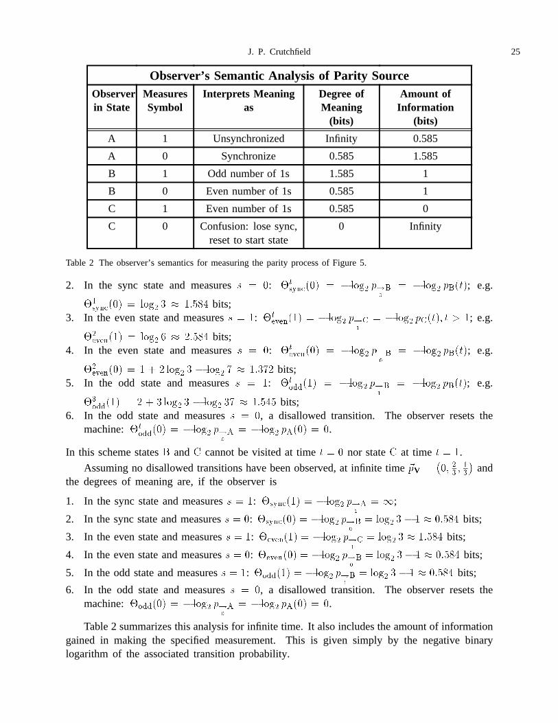
Table 2 summarizes this analysis for infinite time. It also includes the amount of informationgained in making the specified measurement. This is given simply by the negative binarylogarithm of the associated transition probability.
26 Semantics and Thermodynamics
Similar definitions of meaning can be developed between any two levels in a reconstructionhierarchy. The example just given concerns the semantics between the measurement symbollevel and the stochastic finite automaton level.11 Meaning appears whenever there is a changein representation of events. And if there is no change, e.g. a measurement in considered onlywith respect to the population of other measurements, an important special case arises.
In this view Shannon information concerns degenerate meaning: that obtained within thesame representation class. Consider the information of events in some set� of possibilities whoseoccurrence is governed by arbitrary probability distributions����� � � ��. Assume that no furtherstructural qualifications of this representation class are made. Then the Shannon self-information� ��� ��� �� � �� gives the degree of meaning� ���
���
�
� in the observed event� with respect
to total ignorance. Similarly, the information gain��� ��� ��
���
�� ��������
gives the average
degree of “meaning” between two distributions. The two representation levels are degenerate:both are the events themselves. Thus, Shannon information gives the degree of meaning of anevent with respect to the set� of events and not with respect to an observer’s internal model;unless, of course, that model is taken to be the collection of events as in a histogram or look-up table. Although this might seem like vacuous re-interpretation, it is essential that generalmeaning have this as a degenerate case.
The main components of meaning, as defined above should be emphasized. First, likeinformation it can be quantified. Second, conventional uses of Shannon information are anatural special case. And third, it derives fundamentally from the relationshipacross levelsof abstraction. A given message has different connotations depending on an observer’s modeland the most general constraint is the model’s level in a reconstruction hierarchy. When modelreconstruction is considered to be a time-dependent process that moves up a hierarchy, then thepresent discussion suggests a concrete approach to investigating adaptive meaning in evolutionarysystems: emergent semantics.
In the parity example above I explicitly said what a state and a measurement “meant”.Parity, as such, is a human linguistic and mathematical convention, which has a compellingnaturalness due largely to its simplicity. A low level organism, though, need not have such aliterary interpretation of its stimuli. Meaning of (say) its model’s states, when the state sequenceis seen as the output of a preprocessor,§ derives from the functionality given to the organism, asa whole and as a part of its environment and its evolutionary and developmental history. Saidthis way, absolute meaning in nature is quite a complicated and contingent concept. Absolutemeaning derives from the global structure developed over space and through time. Nonetheless,the analysis given above captures the representation level-to-level origin of “local” meaning.The tension between global and local entities is not the least bit new to nonlinear dynamics.Indeed, much of the latter’s subtlety is a consequence of their inequivalence. Analogous insightsare sure to follow from the semantic analysis of large hierarchical processes.
§ This preprocessor is a transducer version of the model that takes the input symbols and outputs stringsin the state alphabet�.
J. P. Crutchfield 27
Machine Thermodynamics
The atomistic view of nature, though professed since ancient times, was largely unsuccessfuluntil the raw combinatorial complication it entailed was connected to macroscopic phenomena.Founding thermodynamics on the principles of statistical mechanics was one of, if not the major,influence on its eventual acceptance. The laws of thermodynamics give the coarsest constraintson the microscopic diversity of large many-particle systems. This same view, moving frommicroscopic dynamics to macroscopic laws, can be applied to the task of statistical inferenceof nonlinear models. And so it is appropriate after discussing the “microscopic” data ofmeasurement sequences and the reconstruction of “mesoscopic” machines from them, to endwith a discussion at the largest scale of description: machine thermodynamics. This gives aconcise description of the structure of the infinite set of infinite sequences generated by a machineand also of their probabilities. It does this, in analogy with the conventional thermodynamictreatment of microstates, by focusing on different subsets of allowed sequences.
The first step is the most basic: identification of the microstates. Consistent with machinereconstruction’s goal to approximate a process’s internal states, microstates in modeling are theindividual measurement subsequences.|| Consider the set������� of all length� subsequencesoccurring in a length� data stream�. The probability of a subsequence� � ������� isestimated by�� � �����, where�� is the number of occurrences of� in the data stream.The connection with the physical interpretation of thermodynamics follows from identifying amicrostate’s energy with its self-information
�� � � ��� �� (35)
That is, improbable microstates have high energy. Energy macrostates are then given bygrouping subsequences of the same energy into subsets�� � �� � � � � ��������. At thispoint there are two distributions: the microstate distribution and an induced distribution overenergy macrostates. Their thermodynamic structure is captured by the parametrized microstatedistribution
����� ������
�����(36)
where� accentuates or attenuates a microstate’s weight solely according to its energy. This isthe same role (inverse) temperature plays in classical thermodynamics. The partition function
����� ��
���������
����� ��
���������
��� (37)
gives the total signal space volume of the distribution���� � ������ � � � ��������. In thisway statistical mechanics explains thermodynamic properties as constraints on how this volumechanges under various conditions.
|| Going from individual measurements in a data stream to subsequences is a change in representationfrom the raw data to the parse tree, a hierarchical data structure.
28 Semantics and Thermodynamics
From these definitions an extensive, system-size-dependent thermodynamics follows directly.For example, given an infinitely long data stream� the average total energy in all length�sequences is
���� ��
���������
������� � ����
�
���������
�������
���� � �����
�
���������
����� ���� �� (38)
And the thermodynamic entropy is given by
��� � �������
�� �
�
���������
����� ���� ����� (39)
where�������
�is the Shannon information of the microstate distribution.
These are definitions of the extensive,�-dependent thermodynamic parameters for a closedsystem thermally coupled to its environment. The total energy� exists in several forms. Themost important of which is the thermal energy, where is the thermodynamic entropy andis the temperature. The remaining “free” energy is that which is stored via a reversible processand is retrievable by one. For a closed and nonisolated system it is the Helmholtz free energy�. The fundamental equation expressing energy conservation is then
� � � � (40)
In modeling, an observer is put into contact with the process and attempts, by collectingmeasurements and estimating models, to come to “inferential” equilibrium by finding the optimalmodel. The above thermodynamics describes the situation where the information in the datastream exists in two forms. The first is that which is randomized and the second is that responsiblefor the deviation from equilibrium. The thermodynamic analog of the Helmholtz free energy is
���� � ���� ���� ����� (41)
It measures the amount of nonrandom information in the ensemble described by����� at thegiven temperature���.
There are three temperature limits of interest in which the preceding thermodynamics canbe simply described.
1. Equilibrium, � � : The original subsequence distribution is recovered:�� � ��� � and�� � . All of the information is “thermalized”�� � ���� and the Helmholtz free energyvanishes���� � �.
2. Infinite temperature,� � �: All microstates are “excited” and are equally probable:����� � ��� , where the partition function is equal to the total number of microstates:� � ���������. The effective signal space volume is largest in this limit. The averageenergy is just the sum of the microstate energies:�� � ���
���. The entropy simply
depends of the multiplicity of microstates� � ���� ���������. The free energy diverges.3. Zero temperature,� ��: The least energetic, or most probable, microstate�� dominates:
�� � ��� , the signal space volume is the smallest�� � �, �� � ��� , and the entropyvanishes� � �.
J. P. Crutchfield 29
The goal for an observer is to build a model that reproduces the observed data stream,including the probability structure of the latter. In thermodynamic terms, the model shouldminimize the Helmholtz free energy. This is what machine reconstruction produces: a stochasticautomaton that is in inferential equilibrium with the given data. How it does this is describedelsewhere.16 The following will cover the basic methods for this, using them to investigate thethermodynamic structure of a machine’s invariant subsequences and distributions.
Dividing each of the extensive quantities by the volume� yields thermodynamic densities.And upon taking the thermodynamic limit of the densities, the asymptotic growth rates of theextensive parameters are obtained. These growth rates are intensive. They can be directlycomputed from the reconstructed machine. In a sense the machine itself is an intensivethermodynamic object: the effective computational equations of motion.
To obtain the intensive thermodynamics from a given stochastic machine� with � ��� ��� � � � �
�, a new set
������
� � � ��
of parametrized transition matrices are defined by
������
����
� ����
��
�
��
(42)
where����
�� � � ���� ����
�� is the information obtained on making the transition from state�
to state�� on symbol�. Note that as the parameter is varied the transition probabilities inthe original machine are given different weights while the overall “shape” of the transitions ismaintained. This is the intensive analog of the effect has on the extensive distribution� above.
Most of the thermodynamic properties are determined by the parametrized connection matrix
�� �����
�����
(43)
There are two quantities required from this matrix. Its principal eigenvalue
�� � ����������������
��� � ������ � ������
�(44)
and the associated right eigenvector� �
��� � � ��� � (45)
Note, however, that�� is not a stochastic matrix. In fact,
�����
���
���
��� �
� �
� �
(46)
It does not directly describe, for example, the probabilities of the subset of sequences that areassociated with the relative transition weightings at the given; except, of course, at � .
There is, however, an “equilibrium” machine, whose stochastic connection matrix is denoted��, that produces the same sequences but with the relative weights given by��. Recall that thestate of macroscopic equilibrium is determined by one of the variational principles:
1. At given total entropy, the equilibrium state minimizes the energy;2. At given total energy, it maximizes the thermodynamic entropy.
30 Semantics and Thermodynamics
Using the latter entropy representation, the equilibrium machine is that with maximal thermo-dynamic entropy subject to the constraints imposed by��. That is, all of the nonzero edgeprobabilities are allowed to vary.�� describes the process over the allowed subsequences whichare in thermodynamic equilibrium at the given temperature. It is found using Shannon’s entropymaximization formula35,40
�� �����������������
��(47)
where����� is a diagonal matrix with the components of�� on the diagonal. Since this is astochastic matrix its principal eigenvalue is unity. However, the associated left eigenvector���
����� � ��� (48)
when normalized in probability gives the asymptotic state distribution.
The entropy rate, as seen in a previous section, is
�����
���
���
���
����
����� ���� ����� (49)
where����� ����
����
. The -complexities are given by
� � �
�
���
�� ���� ��
�� � �
�
���
�� ���� �� (50)
where��������� � ������� . The metric� � �� and topological� � �� quantities are directlyrecovered. That is,
� � �� and � �
�� � �� and� � � (51)
The relation
�� � � ��
���
�(52)
again constrains the entropy rate and the complexities.
Physically speaking����� � � ���� ����� plays the role of an interaction energy betweentwo states and is related to the inverse temperature. Although the same support, i.e. set ofsequences and topological machine, exists at all temperatures, varying accentuates the measureof the process�� over different paths in the machine or, equivalently, over different subsets ofsequences. One subset’s weight changes relative to others as dictated by��’s elements.
J. P. Crutchfield 31
In the limit of long sequences the partition function’s growth rate is governed by the maximaleigenvalue�� of the machine matrix��. That is,
����� ����
��� (53)
The machine Helmholtz free energy density becomes
� � � ������
�
���� ��� �����
� � ���� ��� �� (54)
and the thermodynamic entropy is
� ���������
�(55)
where�� is Boltzmann’s constant. Using the basic thermodynamic relation between these, thetotal energy density is then readily computed by noting
� � � �
� � ������
���
�� ��
���
�(56)
using the identification��� � ��� .
In the entropy representation, the function���, computed from Eq. (55) and Eq. (56),determines the thermodynamic “potential” along an arc�� in the model space� of consistentstochastic machines. Consistent machines are those having the same set of allowed sequences asthose observed in the data stream. At each fixed� the equilibrium machine is estimated via Eq.(47). Here equilibrium refers to a closed and isolated system specified by a fixed temperature andso a fixed average energy�. In contrast, the graph of��� concerns a closed, but nonisolatedsystem in contact with an energy reservoir at temperature��� � �. It gives the entropiesand energies for the family of machines��. The equilibrium machine occurs at� � � wherethe free energy vanishes and all of the unconstrained information is “thermal” or randomized.
This is the thermodynamic analog of a cost function like that over model space� as shownin Figure 3. It is not the same, however, since (i)��� is computed in the thermodynamic limitsof a long data stream and long sequence length and (ii) it represents two different optimizations,one at each temperature and the other over all temperatures. This is the view of statisticalestimation developed in large deviation theory.8,17 It suggests a rather different appreciationof the Sinai-Ruelle-Bowen thermodynamic formalism6,33,39for invariant measures of dynamicalsystems as a foundation for nonlinear modeling.
Independent of this modeling interpretation Eq. (55) and Eq. (56) give a direct way to studymacroscopic properties of the sequences produced by a stochastic machine. In particular, theshape of��� determines the variation in entropy and energy within subsets of sequences that
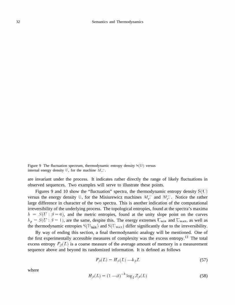
32 Semantics and Thermodynamics
Figure 9 The fluctuation spectrum, thermodynamic entropy density���� versusinternal energy density�, for the machine��
�� .
are invariant under the process. It indicates rather directly the range of likely fluctuations inobserved sequences. Two examples will serve to illustrate these points.
Figures 9 and 10 show the “fluctuation” spectra, the thermodynamic entropy density����versus the energy density�, for the Misiurewicz machines��
�� and��
�� . Notice the rather
large difference in character of the two spectra. This is another indication of the computationalirreversibility of the underlying process. The topological entropies, found at the spectra’s maxima� � ��� � � � ��, and the metric entropies, found at the unity slope point on the curves�� � ��� � � � ��, are the same, despite this. The energy extremes���� and����, as well asthe thermodynamic entropies������� and������� differ significantly due to the irreversibility.
By way of ending this section, a final thermodynamic analogy will be mentioned. One ofthe first experimentally accessible measures of complexity was the excess entropy.13 The totalexcess entropy����� is a coarse measure of the average amount of memory in a measurementsequence above and beyond its randomized information. It is defined as follows
����� � ������ ��� (57)
where����� � ��� ���� �� ���� (58)
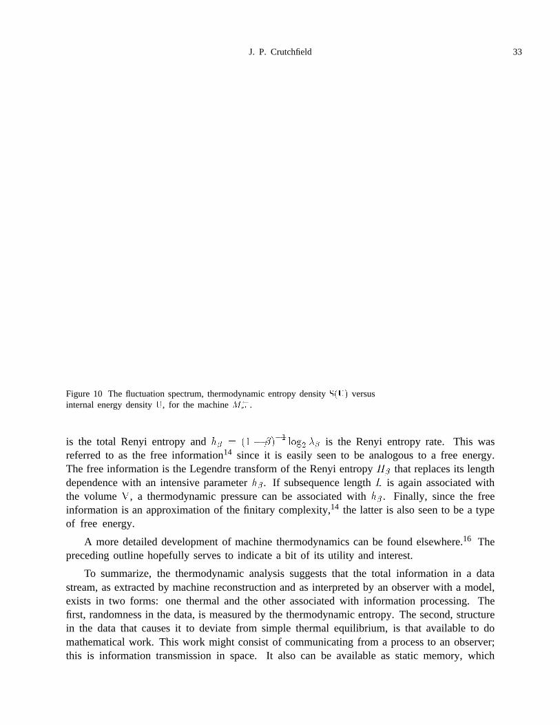
J. P. Crutchfield 33
Figure 10 The fluctuation spectrum, thermodynamic entropy density���� versusinternal energy density�, for the machine��
�� .
is the total Renyi entropy and�� � �� � ���� ������ is the Renyi entropy rate. This was
referred to as the free information14 since it is easily seen to be analogous to a free energy.The free information is the Legendre transform of the Renyi entropy�� that replaces its lengthdependence with an intensive parameter��. If subsequence length� is again associated withthe volume�, a thermodynamic pressure can be associated with��. Finally, since the freeinformation is an approximation of the finitary complexity,14 the latter is also seen to be a typeof free energy.
A more detailed development of machine thermodynamics can be found elsewhere.16 Thepreceding outline hopefully serves to indicate a bit of its utility and interest.
To summarize, the thermodynamic analysis suggests that the total information in a datastream, as extracted by machine reconstruction and as interpreted by an observer with a model,exists in two forms: one thermal and the other associated with information processing. Thefirst, randomness in the data, is measured by the thermodynamic entropy. The second, structurein the data that causes it to deviate from simple thermal equilibrium, is that available to domathematical work. This work might consist of communicating from a process to an observer;this is information transmission in space. It also can be available as static memory, which
34 Semantics and Thermodynamics
is information transmission across time. Most usefully, it can be available to do genuinecomputation and to support thereby semantic information processing.
SCIENCE AS DATA COMPRESSION?
Thinking back to the explanatory channel, these considerations lead me to disagree with thephilosophical premise implicit in the universal coding theory approach to nonlinear modeling.While I accept the mathematics and use the optimization criteria, its own semantics appearswanting. Science is not data compression. The structure of models is ultimately more importantthan their use in encoders and decoders for the efficient encapsulation of experience. In the limitof large data streams and positive entropy processes, i.e. the realm of universal coding theory,the model is essentially ignored and prediction error dominates. At the end of the day, though,good models are independent of the amount of data used to originally infer to them.# This pointwas emphasized in the preceding by the analysis of the effects their computational structurehad on knowledge relaxation and on their semantic structure. Even these naked, mathematicalobjects, with which one typically does not associate meaning, do imply a semantic structure forthe act of measurement. And it is this semantics that gives models their scientific value.
The preceding discussion, though only an outline, attempted to put these issues in asufficiently large arena so that they can stand on their own. At the beginning there are dynamicalsystems whose diverse and complicated phenomenology has rapidly become better understood.They enrich our view of natural phenomena; though they do not necessarily deepen it. Thecontrast between their often simple specification and their creation of apparent complexity leadsto computational mechanics. Computation theory in this development appears as the theoryparexcellenceof structure. During the 1960’s it gave the foundation for a theory of randomness. Butthat success should not blind us to the pressing need for constructive measures of complexity forphysical, chemical, biological, and economic systems that go beyond randomness. Descriptionsof complexity need not always pay for randomness. This is as true of statistical inference appliedto nonlinear modeling as it is of thermodynamic and evolutionary systems. Indeed, it is oneof the primary lessons of nonlinear dynamics that effective randomness is cheap and easilyregenerated. Concomitantly, it also shows that ideal randomness is just that: an ideal that isexpensive and, in principle, impossible to objectively obtain. Fortunately, nature does not seemto need it. Often only randomness effective for the task at hand is required.
This tension between randomness and order, the result of which is complexity, has alwaysbeen a part of the problem domain of thermodynamics. Indeed, phase transitions and, especially,critical phenomena are the primary evidence of nature’s delicate balance between them. Giventhis observation, the question now presents itself to nonlinear modeling, What types of com-putation are supported by physical systems at phase transitions, at the interface between orderand chaos?** Away from “critical” processes, classical thermodynamics forms a solid basis onwhich to build nonlinear modeling. To the extent Gibbsian statistical mechanics is successful,
# To describe the behavior of a thermodynamic system it suffices to communicate the equations ofstate, approximate macroscopic parameters, and possibly the force laws governing the microscopicconstituents. Exact description is not only undesirable, but well nigh impossible.
** A first, constructive answer can be found elsewhere.15
J. P. Crutchfield 35
so too will optimal modeling be. Though, as I just mentioned, there is much to question withinthis framework. Having described the analogy between thermodynamics and optimal modeling,another deeper problem suggests itself.
Classical thermodynamics foundered in its description of critical phenomena due to itsconfusion of the (observable) average value of the order parameter with its most likely value.So too the universal coding theoretic association of the optimal model with the most likely,Eq. (7), can fail for processes with either low entropy or near phase transitions. This will beespecially exaggerated for “critical” processes that exhibit fluctuations on all scales. In thesecases, fluctuations dominate behavior and averages need not be centered around the most likelyvalue of an observable. This occurs for high complexity processes, such as those described bystochastic context-free and context-sensitive grammars,15,30 since they have the requisite internalcomputational capacity to cause the convergence of observable statistics to deviate from the Lawof Large Numbers.
Having told this modeling story somewhat briefly, I hope it becomes at least a littleclearer how the view of microscopic processes offered by statistical mechanics needs to beaugmented. The examples analyzed demonstrate that the computational structure and semanticcontent of processes are almost entirely masked and cannot be articulated within the conventionalframework. But it is exactly these properties that form the functional substrate of learningand evolutionary systems. The claim here is that an investigation of the intrinsic computationperformed by dynamical systems is a prerequisite for understanding how physical systemsmight spontaneously take up the task of modeling their nonlinear environments. I believethe engineering by-products of this program for forecasting, design, and control, will follownaturally.
The greatest sorcerer [writes Novalis memorably] would be the one who bewitched himselfto the point of taking his own phantasmagorias for autonomous apparitions. Would not thisbe true of us?
J. L Borges, “Avatars of the Tortoise”, page 115.5
ACKNOWLEDGEMENTS
I would like to express my appreciation for discussions with Karl Young and Jim Hanson.Many thanks are due to the Santa Fe Institute, where the author was supported by a RobertMaxwell Foundation Visiting Professorship, for the warm hospitality during the writing ofthe present review. Funds from ONR contract N00014-90-J-1774, NASA-Ames UniversityInterchange NCA2-488, and the AFOSR, also contributed to this work.
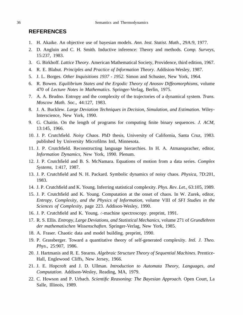
36 Semantics and Thermodynamics
REFERENCES
1. H. Akaike. An objective use of bayesian models.Ann. Inst. Statist. Math., 29A:9, 1977.
2. D. Angluin and C. H. Smith. Inductive inference: Theory and methods.Comp. Surveys,15:237, 1983.
3. G. Birkhoff.Lattice Theory. American Mathematical Society, Providence, third edition, 1967.
4. R. E. Blahut.Principles and Practice of Information Theory. Addision-Wesley, 1987.
5. J. L. Borges.Other Inquisitions 1937 - 1952. Simon and Schuster, New York, 1964.
6. R. Bowen.Equilibrium States and the Ergodic Theory of Anosov Diffeomorphisms, volume470 of Lecture Notes in Mathematics. Springer-Verlag, Berlin, 1975.
7. A. A. Brudno. Entropy and the complexity of the trajectories of a dynamical system.Trans.Moscow Math. Soc., 44:127, 1983.
8. J. A. Bucklew.Large Deviation Techniques in Decision, Simulation, and Estimation. Wiley-Interscience, New York, 1990.
9. G. Chaitin. On the length of programs for computing finite binary sequences.J. ACM,13:145, 1966.
10. J. P. Crutchfield.Noisy Chaos. PhD thesis, University of California, Santa Cruz, 1983.published by University Microfilms Intl, Minnesota.
11. J. P. Crutchfield. Reconstructing language hierarchies. In H. A. Atmanspracher, editor,Information Dynamics, New York, 1990. Plenum.
12. J. P. Crutchfield and B. S. McNamara. Equations of motion from a data series.ComplexSystems, 1:417, 1987.
13. J. P. Crutchfield and N. H. Packard. Symbolic dynamics of noisy chaos.Physica, 7D:201,1983.
14. J. P. Crutchfield and K. Young. Inferring statistical complexity.Phys. Rev. Let., 63:105, 1989.
15. J. P. Crutchfield and K. Young. Computation at the onset of chaos. In W. Zurek, editor,Entropy, Complexity, and the Physics of Information, volume VIII of SFI Studies in theSciences of Complexity, page 223. Addison-Wesley, 1990.
16. J. P. Crutchfield and K. Young.�-machine spectroscopy. preprint, 1991.
17. R. S. Ellis.Entropy, Large Deviations, and Statistical Mechanics, volume 271 ofGrundlehrender mathematischen Wissenschaften. Springer-Verlag, New York, 1985.
18. A. Fraser. Chaotic data and model building. preprint, 1990.
19. P. Grassberger. Toward a quantitative theory of self-generated complexity.Intl. J. Theo.Phys., 25:907, 1986.
20. J. Hartmanis and R. E. Stearns.Algebraic Structure Theory of Sequential Machines. Prentice-Hall, Englewood Cliffs, New Jersey, 1966.
21. J. E. Hopcroft and J. D. Ullman.Introduction to Automata Theory, Languages, andComputation. Addison-Wesley, Reading, MA, 1979.
22. C. Howson and P. Urbach.Scientific Reasoning: The Bayesian Approach. Open Court, LaSalle, Illinois, 1989.
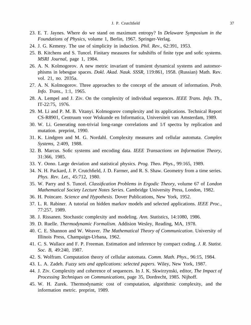
J. P. Crutchfield 37
23. E. T. Jaynes. Where do we stand on maximum entropy? InDelaware Symposium in theFoundations of Physics, volume 1, Berlin, 1967. Springer-Verlag.
24. J. G. Kemeny. The use of simplicity in induction.Phil. Rev., 62:391, 1953.
25. B. Kitchens and S. Tuncel. Finitary measures for subshifts of finite type and sofic systems.MSRI Journal, page 1, 1984.
26. A. N. Kolmogorov. A new metric invariant of transient dynamical systems and automor-phisms in lebesgue spaces.Dokl. Akad. Nauk. SSSR, 119:861, 1958. (Russian) Math. Rev.vol. 21, no. 2035a.
27. A. N. Kolmogorov. Three approaches to the concept of the amount of information.Prob.Info. Trans., 1:1, 1965.
28. A. Lempel and J. Ziv. On the complexity of individual sequences.IEEE Trans. Info. Th.,IT-22:75, 1976.
29. M. Li and P. M. B. Vitanyi. Kolmogorov complexity and its applications. Technical ReportCS-R8901, Centruum voor Wiskunde en Informatica, Universiteit van Amsterdam, 1989.
30. W. Li. Generating non-trivial long-range correlations and 1/f spectra by replication andmutation. preprint, 1990.
31. K. Lindgren and M. G. Nordahl. Complexity measures and cellular automata.ComplexSystems, 2:409, 1988.
32. B. Marcus. Sofic systems and encoding data.IEEE Transactions on Information Theory,31:366, 1985.
33. Y. Oono. Large deviation and statistical physics.Prog. Theo. Phys., 99:165, 1989.
34. N. H. Packard, J. P. Crutchfield, J. D. Farmer, and R. S. Shaw. Geometry from a time series.Phys. Rev. Let., 45:712, 1980.
35. W. Parry and S. Tuncel.Classification Problems in Ergodic Theory, volume 67 ofLondonMathematical Society Lecture Notes Series. Cambridge University Press, London, 1982.
36. H. Poincare.Science and Hypothesis. Dover Publications, New York, 1952.
37. L. R. Rabiner. A tutorial on hidden markov models and selected applications.IEEE Proc.,77:257, 1989.
38. J. Rissanen. Stochastic complexity and modeling.Ann. Statistics, 14:1080, 1986.
39. D. Ruelle.Thermodynamic Formalism. Addision Wesley, Reading, MA, 1978.
40. C. E. Shannon and W. Weaver.The Mathematical Theory of Communication. University ofIllinois Press, Champaign-Urbana, 1962.
41. C. S. Wallace and F. P. Freeman. Estimation and inference by compact coding.J. R. Statist.Soc. B, 49:240, 1987.
42. S. Wolfram. Computation theory of cellular automata.Comm. Math. Phys., 96:15, 1984.
43. L. A. Zadeh.Fuzzy sets and applications: selected papers. Wiley, New York, 1987.
44. J. Ziv. Complexity and coherence of sequences. In J. K. Skwirzynski, editor,The Impact ofProcessing Techniques on Communications, page 35, Dordrecht, 1985. Nijhoff.
45. W. H. Zurek. Thermodynamic cost of computation, algorithmic complexity, and theinformation metric. preprint, 1989.
Recommended