Space-Time Filtering, Sampling and Motion Uncertainty
Radu S. Jasinschi
CMU-RI-TR-88-9
The Robotics Institute Carnegie Mellon University
Pittsburgh, Pennsylvania 15213
June 1988
0 1988 Carnegie Mellon University
This research was supported by the Defense Advanced Research Projects Agency @OD), monitored by the U.S. Army Engineer Topographic Laboratories under Contract DACA 76-85-C-OOO2.
Address: Center for Automation Research, University of Mayland, College Park, MD 20742

Abstract
We analyse the structure of filters which are space-time oriented. Basically, this paper consists of two parts. In the first one, we present the cascade of space-time DOG as an energy filter, discuss its general properties and show how to compute its energy. In the second part, we discuss the consequences of applying the sampling theorem to uniformly translating patterns in the presence of motion uncertainty. It is shown that, for a given motion uncertainty, there exists a bound on the maximum sampling interval, such that for larger values aliasing will occur.


1 INT.RODUCl7ON
1 Introduction
1
The problem of the extraction of the optical flow has, in recent ytats, been treated from a new point
of view, that is, through the use of space-time filters [7,4,6,5]. The basic idea behind this method
is to extract the optical flow without having to perform any type of operation other than to use a
collection of filters which arc tuned to different orientations in space-time (or equivalently in the
frequency domain). Also, given that the outputs of these filters have been computed, it is necessary
to establish a method by which we can determine the value of the tstimatcd optical flow, because
the output of a filter tuned to a specific orientation (even if with maximal rtspanse) is not enough to
extract the optical flow and wc have to use a complete set of filters (in the scnsc that it takes into
account all possible orientations). In space-time filtering, we umvolve a squencc of images with a
(space-time) filter, such that the interval h w e m SuccSSive images is small. Thc minimum temporal
interval between sucessive images is basically dictated by practical considerations, because if it is too
small wc get little amount of information about the moving pattern from frame to frame. On the other
hand, we would like to know what the value of the maximum temporal interval between sucessive
images should be such that wc umtinue to be able to use a filtering approach to the extraction of
optical flow
The answer to this question comes by considering the sampling issues involved in this filtering
proctss. As I will show in section 3, if the= exists a certain degree of motion uncertainty, then
the maximum sampling interval. is fixed by this motion uncertainty. This means that the= exists a
(non-linear) relatiamhip between the motion uncertainty and the maximum sampling interval.
The procedure of using a collection of filters to extract optical flow corresponds, in a general
SCIISC, to a signal processing approach, which is mainly concerned with the extraction of information
about the original signal, in the p m c e of noise. It involves the construction of filters, if possible
optimal ones, parameter estimation and the analysis of sampling issues.
On the other hand, in the feature based approach to the extraction of optical flow [3] it is necessary
to, previously to the actual computation of of the optical flow, extract edges (zero crossings) which

2 SPACE-TIME FILTERING 2
have to be matched in suctssive fhmes. If the temporal intend between succesive images is large
and the number of edges to be matched between frames is not high, then a contour-based approach
can be sucessful in extracting the optical flow. But, on the other hand, if the number of edges is
large, the amount of mismatchings can lead to a high rate of error, and as a consequence of this to a
wrong estimation of the optical flow.
It is therefore important to be able to detect moving fcatuns and extract their optical flow in
the presence of noisy data and imprecise measurements. Depending on the spatial complexity of
information available at each image, in the temporal sequence of images, it can be more reliable to
use a filtering approach, especially for the casc in which the interval between these images is small
and them exits a high spatial content of infomation (which makes a featwe matching approach highly
unstable).
In this paper we discuss, in d o n 2, the issue of extracting the optical flow through feature
or intensity based approaches versus space-time filtering, and present the space-time DOG cascade
as an energy filter. In d o n 3 we analyst sampling issues which apply for uniformly translating
patterns in the presence of noise (motion uncertainty). Finally, we draw conclusions in d o n 4,
and make an analogy between the long and short-range processes of motion extraction in the human
visual systtm and the feature-based and space-time filtering methods in Computer Vision.
2 Space-time filtering
2.1 Extraction of the optical flow in intensity and feature-based approach
The extraction of the optical flow field fran the intensity variations in the image plane has been mated
until very recently, in Computer Vision, as a feature or intensity-based problem. In the feature-based
approach we have to detect relevant features, such as edges, from a pair of succssive images (in
a temporal sequence of images), and afterwards perform a matching of corresponding elements, so
2 SPACE-TIME FILTERING 3
that, as a d t of this proctdurt, we assign a specific value of the optical flow to the corresponding
elements.
This method has to overcome two major problems:
1. The correspondence problem
2. The apexture problem.
The correspondence problem [l] addresses the question of how to assign the same identity for
elements which appear in temporal rmccssioa of images. The contspondence, or matching, can be
computed in different ways. depending, in part, on the temporal interval between succtsive images.
If this interval is small, the wmspondence between features can be performed through a set of local
opemions over elements which are spatially close to each other. One of these operations [1,17]
consists in the minimiion of the distance a set of elements takes to travel fnnn one image to its
mrctssive me. On the other hand, if this temporal interval is large, it is more likely that a more
global type of operation for the matching of fcaturcs has to be implemented. In general, the matching
of corresponding elements in suctssive images c a ~ ~ be unstable, due to noise in the image, and also
computationally expensive if the number of features to be matched is large.
In respect to the ape- problem, which states that it is not possible to measwe both components
of the optical flow field given a small ape- in the image, we have to inmduce additional conmints
into the model describing the extraction of Optical flow, so as to make it possible to obtain the
full optical flow field. Actually, given a small apcrwt, we are only able to measwe the normal
component (to the gradient of the intensity) of optical flow field, while its tangential component
mains undetermined. As one example of the solution to the aperrurt problem, we can mention the
area-based [2] formulation which assumes the use of a smoothntss term, in addition to the intensity
continuity equation, represented by the sum of the squaxw of the spatial derivatives of the optical flow
field components. Another example is given by the contaur-bastd [3] approach, wheE the mntraint
is represented by the gradient in respect to the arc length along the intensity gradient of the optical

2 SPACE-TIME FILTERING 4
flow field, in addition to the difference between the normal component of the optical flow and its
measured value.
Both, the comspondence and the aperture problem, involve in practice a artain amount of
arbitrariness in t e r n of having to choose a set of coI1sv8ln ' ts which enable us to extract the full
optical flow. It is therefore desirable to be able to eliminate the necessity of having to cope with both
of these problems. The method of space-time filtering docs this, in part, by eliminating altogether the
necessity of the use of the comspondcnce problem. In respect to the aperture problem the solution
given by Hccger [SI consists in modeling thc image flow as (locally) purely translational, so that
the optical flow is extracted by fitting a plane to the energy of the filter. This is equivalent to the
computation of both components of the optical flow field, because for translational motion the support
in the frequency domain is given by a plane whose orientation is a function of the velocity vector.
2.2 Space-time oriented iilters
Space-time filtering ccmsists, basically, in the convolution of a temporal sequence of images (closely
displaced) with a (space-time) filter. The most important aspect of space-time filtering lies in the fact
that, if we consider an uniformly translating pattern, we arc able to select a specific velocity by using
(space-time) ori~nttd filttrs [a].
Let us take the example of onedimcnsional motion (in the x direction). If we analysc the picture
which is generated in space-time by an uniformly translating pattern (through a cross-scction parallel
the x-t plane), then we can conclude that the orientation of the individual elements (like lines or
Stripes) is intrinsically determined by the velocity of the pattern (the slopc of a line in the EPI plane
is equal to the velocity of the feature associated to it). A very htemting example of this kind of
relationship between (space-time) orientation and velocity is described by the cpipolar plane images
@PIS) mated by Bollts and Baker [8] for the case of a camera moving (perpcndicularly to the
dirtction of motion) in a static environment. There, at a given EPI, we are able to track the temporal
evolution of each image element (at a fixed height), and this is described by a seaight line.

2 SPACE-TIME FILTERING 5
Once we know that, for uuiform translation, the space-time evolution of image elements is given
by straight lines, in order to select a specific velocity (optical flow), we can use (space-time) oriented
filters [6,7]. A particularly impoxtaut aspect of this analysis comes from the fact that, for an uniformly
translating pattern, the support of the contrast fundon in the fnquency domain is given by a plane
(or a line for the cast of onedimensional motion) [7,10] passing through the origin of the coordinate
system. In t e r n of space-time filtering, this means that, in order to select a specific velocity of an
uniformly translating pattern, we have to tune the filter to the orientation in the fresuency domain
which gives the highest nsponse.
The use of directionally selective (space-time) filters posc a limitation in the sense that they are
phase sensitive (61. This means that, depending on the alignment between the space-time configuration
of moving pattern and the filter shape, wc cau get different results: the filtercd output may oscillate
or vary betweem positive and negative values. A solution to this problem is given by computing the
mergy (power sptcaum) of the filter output. The energy of a convolved signal is independent of any
phase problem, and for thc case of an uniformly translating pattcm its output is constant.
If, for example, we compute the energy associated to a space-time Gabor filter [5] convolved with an arbitrary function, them the final result will not oscilate or depend on any phase factor. This leads
to the concept of space-time oriented filters as energy filters, which, with the assumption of random
texturtd images and Parstval’s theorem made it possible for Httger [5] to, analytically, predict the
mergy assaciatexi to a particular space-time oriented pattern.
2.3 Space!-time Difference-of-Gaussian @OG) cascade as an energy filter
Space-time filtering, either through energy filters or cascades, is primarily concerned with the pro-
cessing of a temporal sequence of images, such that the interval between successive images is small.
On one hand, the wodt of Hecger 151 showed us that it is possible to obtain a dcnse image flow

2 SPACE-TIME FILTERING 6
map by using a collection of twelve space-time Gabor filters, each tuned to a different direction in
space-time. The space-time Gabor filter is parameaized by three (gaussian) filter sizes (ax, uy and
a,), in addition to the (three) sine or cosine space-time frequencies (whose relative ratios correspond
to different orientations in space-time). It would be desirable to have a broader space-time tuning
capability, as, for example, in the case of the cascaded filters proposed by Fleet and Jepxm [9]. They
proposed the construction of space-time oriented filters in terms of cascades of the CS filter. The CS
filter is dehed as the diffeEnce of spatial gaussians which arc each multiplied by a temporal expo-
nentially decaying function, comsponding to a temporal center (C)-surround (S) model, in analogy to
biological systems, plus, a temporal delay term emboddied in the S part. The space-time orientation
is obtained by canvolving the CS filter with a sum of (space-time) Dirac distxibutions, each centered
at a specific location in space-time so that the d t is a oriented pattern. The use of l a y e d cascades
of the CS filter improves the orientation specificity of the filters, as shown by Fleet and Jepson [9].
In respect to its tuning capabilities, these layered cascades of the CS filter, arc able, in addition to
their specific orientation, to select fcaturts moving at high or low speed by adjusting the ratio of the
spatial or temporal filter sizes to one, rtspectively.
We would like to use a filter which exibits a wide range of space-time tuning and can also be used
to extract the image flow as an energy filter. The simplest fusion of these two aspccts is exibited by
the space-time DOG filter, used in cascade. In fact, if we substitute the temporal exponential decay
term in the CS filter by a temporal gaussian, and eliminate the temporal delay, we get a space-time
DOG. The number of parameters of this filter is qual 9, where 4 c~mspond to the center and
rmrround filter sizes (the spatial filter sizes llft assumed to be qual), spatial and temporal offsets
make up 3 parameters, plus the center and surround multiplicative wnstauts. The only FeaSOn for
not using the CS cascade filter of Fleet and Jepson directly as an energy filter comes from the fact
that the energy expnssion nuns out to be more complex than that of the space-time DOG cascade
because it has a linear temporal exponential decay, whereas for the DOG filter the temporal decay is
gaussian, thus making it easier to perfom the temporal integral in ordcr to get the energy expression.
We should remind ourselves that the space-time DOG and Gabor filters an non-causal, as a
consequence of the Paley-Wiener thmrem [121 which states that, if a temporal filterf(t) has a square

2 SPACE-TIME FILTERING
integrable Fourier transform f (w) and satisfies the relation
7
thenf(z) is causal. The CS filter, on the contrary, due to its linear exponential temporal decay, is a
causal filter.
The space-time DOG filter is given by the following expression
where a, (0,) and p, (p,) arc the center (!nmmnd) spatial and temporal filter sizts respectively, while
A, and A, arc adjustable parameters (used in the discrete versim of the filter to tune the sum of all
elements of the mask to zero). Its Fourier transform is given by
where the spatial and temporal fnquencies arc rtsptctively given by k' ( E = (kz, k,)) and w.
A cascade of filters comsponds to applying, in sucession, a set of linear filters, to a collection of
signals [9], such that the intend bttwten their suctssive positions of highest magnitude is measured
by the offset. In the case of space-time filtering these offsets have a spatial as well as a temporal
part. Also, they can occur in a set of layers, where each layer comspoads to a different collection
of space-time offsets.
Lct us define, analogously to Fleet and Jepsan [9], the one-layer cascade by the expression

2 SPACE-TIME FILTERING 8
6(.) is the Dirac delta (distribution), D(x, y , 2) the space-time DOG as given by formula (2.2) and * the convolution operation. In the frequency domain this cascade is given by
e(& w) = &i, w ) &E, w) (2.6)
where
1 1 2 4 1 2
E(i,w) = - + - [ e x p ( i ( Z . f + M)) + c x p < - i ( i . f + M))]
= - [ 1 + w s ( i . f + w r ) ] ,
and &E, w) is given by (2.3).
(2.7)
By increasing (decreasing) the offset values of, for example, the me-layer cascade we get more
(less) specificity to velocity. 'Ihis can be observed by comparing Figurts 1 and 2, or their nspective
Fourier transform, Figures 3 and 4. We fix V, = 1.0, V, = 3.0, M, = 1.0, M, = 3.0, A, = 1.0 and
A, = 1.0.
For Figure 1 we have & = 0.77,6 = 0 and I = 2.89, whercas for Figure 2, & = 0.52, tY = 0
and I = 1.93, which CoilTtspond to a slope of 15 deg in the x-t plane (or 0.26 pixels per frame). If
we inspect Figures 3 and 4 it bccames clear that for larger offsets (F@e 3) we get more tuning to
velocity, although more ringing [9] (due to aliasing of adjacent patterns), for small velocities. A way
by which wc get less ringing and more velocity specificity, as described by Fleet and Jepson [9], is
to build cascades out of mort than m e layer. For example, a two layered cascade is constructed by
convolving two one-layer cascades, each with a different collection of offset values, that is

2 SPACE-TIME FILTERING 9
For this two-layer cascade, Figure 5, and its Fourier transform Figure 6, we can observe (we
use the same space-time scale as for the one-layer cascade Figures) that there occurs much less
ringing ( F i p 6) and its space-time shape exibits a broader (also narrower), support at the particular
orientation for which it is tuned.
In general, irrtspective of the set of parameters that we choose for the filter, there always exits a
specific amount of directional -certainty which is a consequence of the fact that the filter response is
not p e r f d y tuned to a particular orientation. This is a comqucna of the fact that, in addition to the
rtsponsc of the 6lter to the particular orientation for which is tuned, there exists a non-zero respense
to a rcstrictcd range of orientations in its neighborhood. For example, in the case of onedimensional
motion (parallel to the x axis) of a given image pattern, in order to filter the specific direction (in the
x-t plane or, cquivalentIy, in the frcqutncy domain) associated to its velocity, we should use a filter
which exibits its support at a given onentation and is zero otherwise. In practice, we will only be
able to select a given orientation inside a cone, such that its apcxture is proportional to the motion
uncertainty. This is a consequence of the fact that any (real) filter will not only select the particular
direction for which it was &signed, but also adjacent directions h i & a fixed apcxture. As a result
of this, there will always d t a motion uncertainty, and constqucntly, this will affect (space-time)
the sampling pmpcrtics of the filter. This issue will be discussed in detail in the next section.
The energy (power sptctnrm) associated to the one-layer cascade is given by
Since we assume only translational motion, in which case it holds that
- w = k - i ; (2.14)
where i; is the velocity field, we can rewrite the previous energy expression in the following form
10
(2.15)
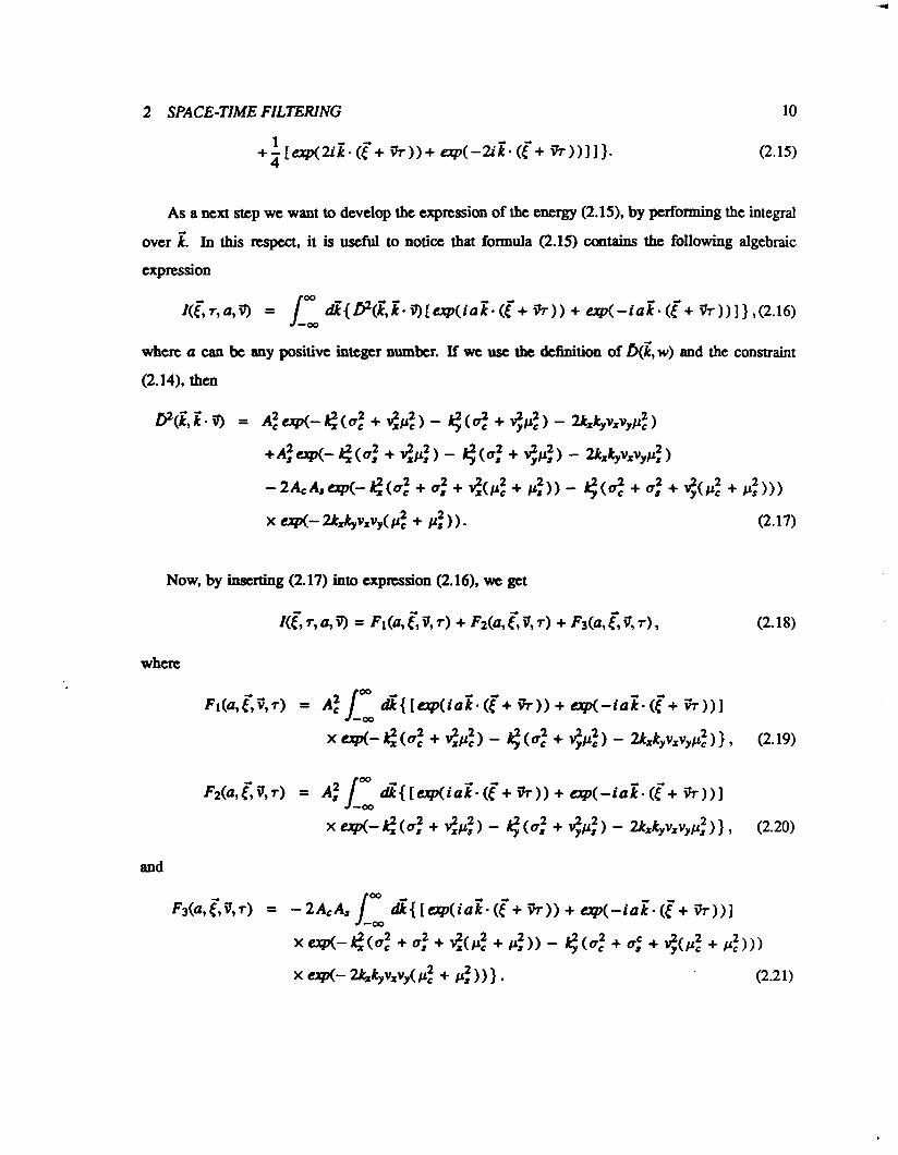
As a next step we want to develop the expression of the energy (2.15). by performing the integral
over E. In this respect, it is useful to notice that formula (2.15) Contains the following algebraic
expression W
1 ( c ~ , a , J ) = lw u%{bZ(E,r-J)[qp(iaZ.(f+ 37)) + qp(-iaZ-(<+ *))]},(2.16)
where a can be any positive integer number. If we usc the definition of 6(z ,w) and the constraint
(2.14), then
Now, by inserting (2.17) into expression (2.16), we get
where
(2.17)
(2.18)
(2.19)
(2.20)
and

2 SPACE-TIME FILTERING
Finally, if we use the (gaussian) integral formula
11
(2.22)
for an arbitrary (2 x 2) matrix A, then F1 will be given by

2 SPACE-TIME FILTERING 12
If we want to extract the optical flow field by using a set of energy filters, each tuned to a different
orientatian in space-time, then we are confronted with another sourct of motion uncertainty. This
comes from the fact that we have to determine the optical flow field, given the output of a number
of energy filters (with different orientations). For example, in Hecger’s approach the estimated field
( v ~ , v,,) minimha a cost function, which consists in the sum of the difference between the mtaSufed
(motion) energy and its predicted value, over all twelve filters. This mcaus that there will always
exist a non-zero contribution from filters which do not correspond to the right orientation, due to an
overlap in the shape of neighboring filters. If wc wish to reduce the uncertainty in the motion estimate
btcause of neighboring mteraction among filters, we have to enhance the orientation specificity of
each filter (thus leading to less lateral overlap). But this has the consequence that, for a fixed number
of filters, some orientation (mainly comsponding to the orientations between that of neighboring
filters) will not be able to be selected any more. So we are faced with a trade-off betwten being
able to select a specific orientation in s p a - h e , with a minimum of uncertainty, and the minimum

3 SPACE-TIME SAMPLING
numbers of filters necessary to span all orientations.
13
The method of optical flow extraction used by Heeger [Z], although it is able to determine the
optical flow for a co l ldon of differtnt types of moving patterns, contains some limitations which
should be mentioned, that is:
1. It assumes that all images can be modeled as (locally) random pattern
2. In order to be able to use ParseVal’s theorem, it is necessary to approximate the expression of
the energy
3. The optimization proctdurt, which has to be perfoxmed at each image pixel, is computationally
very expensive.
In particular, the issue of approximating the integral in parstval’s thtorcm, leads to errors in the
estimated value of the optical flow in regions when it is discontinuous, thus making it difficult to
use the estimated value as input for the operation of region segmentation. This and other questions
will be discussed in another paper [ 111.
3 Space-time sampling
In the previous section I discussed the qucstion of extracting the optical flow by using space-time
filters, considertd as energy filters. Also, I proposed the use of cascades of space-time filters like the
ones constructed by Flea and Jcpson as energy filters, which can be accomplished by substituting the
temporal exponential by a gaussian. A c~nsequence of adopting a filtering approach to the extraction
of the optical flow is the fact that it is necessary to sample the filter, or more specifically, to perform
a space-time sampling of the filter. The temporal sampling issue is very cleariy determined by the
fact that the temporal interval bttween sucessive images used in space-time filtering, although mall,

3 SPACE-TIME SAh4PLJNG 14
is finite. A question which is naturally raised in this context is in respect to how much can we
(temporally) undersample the filter, or in a more complete statement, the convolution of the image
sequence With the space-time filter, so that we arc still able to reconsvUct the original signal. For
uniformly translating patterns, the spatial and temporal sampling ratios are not independent, and, as
it is shown next, ifthere exists a certain amount of motion unceItainty, then there exists a maximum
sampling interval, in either space or time, such that aliasing does not occur. This maximum sampling
interval is shown to be a (non-linear) function of the motion uncertainty.
Initially, I will describe very succintly, for one-dimcnsional functions, the sampling theorem and
generalize it to thrtc-dimcnsions (two spatial and one temporal). Next, I show that for an uniformly
translating pattcm it is only xmxsaq to sample in either the spatial or temporal variables. Fiially,
I relate motion uncertainty with the maximum sampling interval such that there is no aliasing.
The sampling t h e o m [12] gives us a mathematical formulation for the nconstruction of a con-
tinuous function in terms of a collection of samples of this function, over a specific domain. If we
deal with real signals, on tbc other hand, them is always a certain amount of under or oversampling
depending on the specific archittctun of the filters being used. In particular, for the case of undersam-
pling (where the spatial or temporal sampling rate is larger than the one established by the sampling
theorem - the Nyquist rate), we have to dcal with the aliasing problem. The degree of aliasing which
is permitted (so that it still is possiMc to mxmmuct the original function, modulo small distortions)
depends not only on the filter charsctcristics but also on the type of data being filtered.
Let us start with onedimensional signals, rcprtscnttd by the functionf(x). We obtain a sample
off(x),&(x), by multiplying it by a (infinite) sum of (Dirac) delta distributions, such that the sample
points are equidistant (by px). 'Ihc sample funaionfs(x) is given by
where
3 SPACE-TIME SAMPLJNG
In the frequency domain, (3.1) is reprcsenttd by the convolution
5 (kx ) = P W * m x , P x ) 9
with
15
(3.3)
If we assume thatf(kx) is band-limited ( f (k , ) is zero for lkxl > ;), then it is easy to check
that, unless px 5 &, there will exist a region where the adjacent lobes overlap, which is a signal of
undersampling, and as a c<mstqucnce of this we have the aliasing phenomenon. In order to avoid this
from happening, we multiply formula (3.3) by a function If(&), as for example the ideal low-pass
filter (which is 1 for Ikxl 5 L, and 0 otherwise), as a d t of which (3.3) reduces tor(&). ' Ihis has
the consequcncc thatf(x) can be exactly recovered from its samples. We can synthesize this result,
by stating that, iff&) is band-limited and has no singularitits at its extremeties (kx = j&), then
where sin T X
sinc(x) = -, AX
which is a version of the sampling theom [131.
we can generalize thc sampling thtortm to thFtcdimensimal functions. so, given thatf(x,y, 2)
is a (space-he) function andf(k., A,, w) its Fourier transform (kx, A, and w arc the Fourier variables
associated to X, y and 0, f is zero for lkxl > Lz, 141 > 4 and Iwl > & and it does not have
singularitits at fkl = L 141 = & and IwI = 4, then, by the sampling theorem
The case of translational motion [14,15], in which case it holds that

3 SPACE-TIME SAMPLJNG 16
(which is equivalent to say that w is different from zero only on the plane determined by k'- 3), the
sampling theorem reads
This means that we only need to samplef(x,y), at the Nyquist rate, in terms of its spatial variables.
Another way to understand this issue is given in terms of a fourier analysis, which, as a matter of
simplicity, we apply for the two-dimensional case (x-t space.). We know that for pure translation,
because of formula (3.8). the sampled function$ (kx, w) (analogously to (3.3)) is given by
00 0 0 -
By using that
/&d(x - u ) b ( x - 6 ) = 6(u - 6 ) ,
(3.10)
(3.1 1)
(3.12)
(3.13)
We can conclude that, if we start by assuming thatf(x- vxt) is sampled independently in its spatial
and temporal variables, then, due to the constmint of uniform translation, we IVC led to conclude that

3 SFACE-TIME SAMPLJNG 17
we only need to sample in the spatial (temporal) variable. So, we can simplify equation (3.10) to the
following form 00
L(k,,w) = f ( k , ) w J - kxv,) * r c G N k , - 2 n x L ) l , (3.15) nx=-00
or, by expanding the convolution we get
L(kx,w) = E f ( k ~ - 2nXL)2L,6(w - v x ( k x - 2 n , L ) ) , (3.16)
which leads us to the two-dimensional version of equation (3.9). The expression (3.16) is identical to
the one &scribing the Burr’s exptximent [ 151 which consists in sampling in space, at a hed temporal
imwal, a pattern which moves at umstant rate.
&=-a0
For illustration, if we consider a (space-time) band-limited function which describes an uniformly
translational motion, then, by the constraint (3.8) its support (im frequency domain) is given by a line
segment, as it is shown in Figwe 7. Its sampled version, satisfying equation (3.16) with M, = &, consists of a collection of nplicas of the original line segment, which are unifomly sampled at
intewals of M, (see Figure 8).
From this we can deduce that, once the support of f (k , ) is defined by the straight lines whose
slope is given by v,, its sampling ratc is equal to the spatial sampling rate (or equivalently to the
temporal sampling). The fimctionf(x, t) (which is identical t o f ( x + vxz)) cau be reconstructed from
$ (k,, w) by applying a filter which has a support parallel to the lint w = kv,, and more than this,
as it is shown by Crick et d. [14], this support cau be dud to an infinitesimally n m w strip,
as long as there is no motion uncertainty. This means that, for the case of translational motion, we
can increase the sampling mte p, as much as we wish, given that we arc able to exactly measure
the velocity v,. On the other hand, if we deal with real images, there is always a certain degree of
unccxtainty in the motion mc8suTcmcnt, so that the previous considerations do not hold. This leads
us to the issue of considering the sampling theorem in the presence of noisy data (thus generating
motion uncertainty). As a consequence of this, we have to know in what way the sampling themrem (as
previously described) has to be modified in order be able to deal with motion uncertainty. Specifically,
in the presence of motion uncertainty, it is no longer possible to arbitrarily increase the sampling

3 SPACE-TIME SAiUPLJNG 18
interval, without getting aliasing. This establishes a relationship between the maximum sampling
internal (in space) (or minimal in the fresuency dmain) and motion uncertainty.
We know that under the umditians of translational motion (let consider only onedimensional
motion), the Fourier transform of a space-time function has support at the lines passing through the
origin, and whose slope is proportional to the velocity of the moving pattern. If we introduce a
specific d e p of uncertainty for the velocity, then this support will be given by a (onedimensional)
cone, whose aperture is proportional to the uncertainty in the velocity (See Figurts 9 and 10).
Considering the case of a band-limited function (with finite support in the frequency domain), we
can usc polar coordinatts to d d b e its (two-dimensional) variables.
For the angular variable 8 we have 8 = arctanv, and the radial variable r is the maximum
of $2 +e. me motion llDctRainty AV, is given by AV, = (-(e +A@) - tanel, where Ae
comspomls to the angular apeme of the cone, ccntertd at 8. For small v d ~ e s of Ad, 68, Av, can
be approximattd to 6v, = d e a e .
If we sample f ( x + v,t) dong the x direction in intends of p, (or M, in the fr-equency domain)
Figun lo), then it is easy to show that, for a fixed motion uncertainty, there exists a minimum value
of M,, e, such that the adjacent patterns do not overlap.
If we decrease MI beyond this thrcshold, aliasing occurs. This establishes a relationship between
e and Av,, as shown by the following theorem.
Theorem: If we have a bta&limitcd firnction f (x , t) describing M unjfonnly translating
pattern, given that its velocity v,, which is assumed to be &~erentfrom zero, is measured within
an uncertainty range of Av,, then &re &ts a minimMI value for the spatial frequency sampling
interval e such thm no a l h i n g occurs. e is related to Av, by
2 r s i n ( A 8 / 2 ) m e= tan8 + tan(A8/2) ’

3 SPACE-TIME W P L J N G 19
where
r = -4~2 + e , tane = vx .
proof:
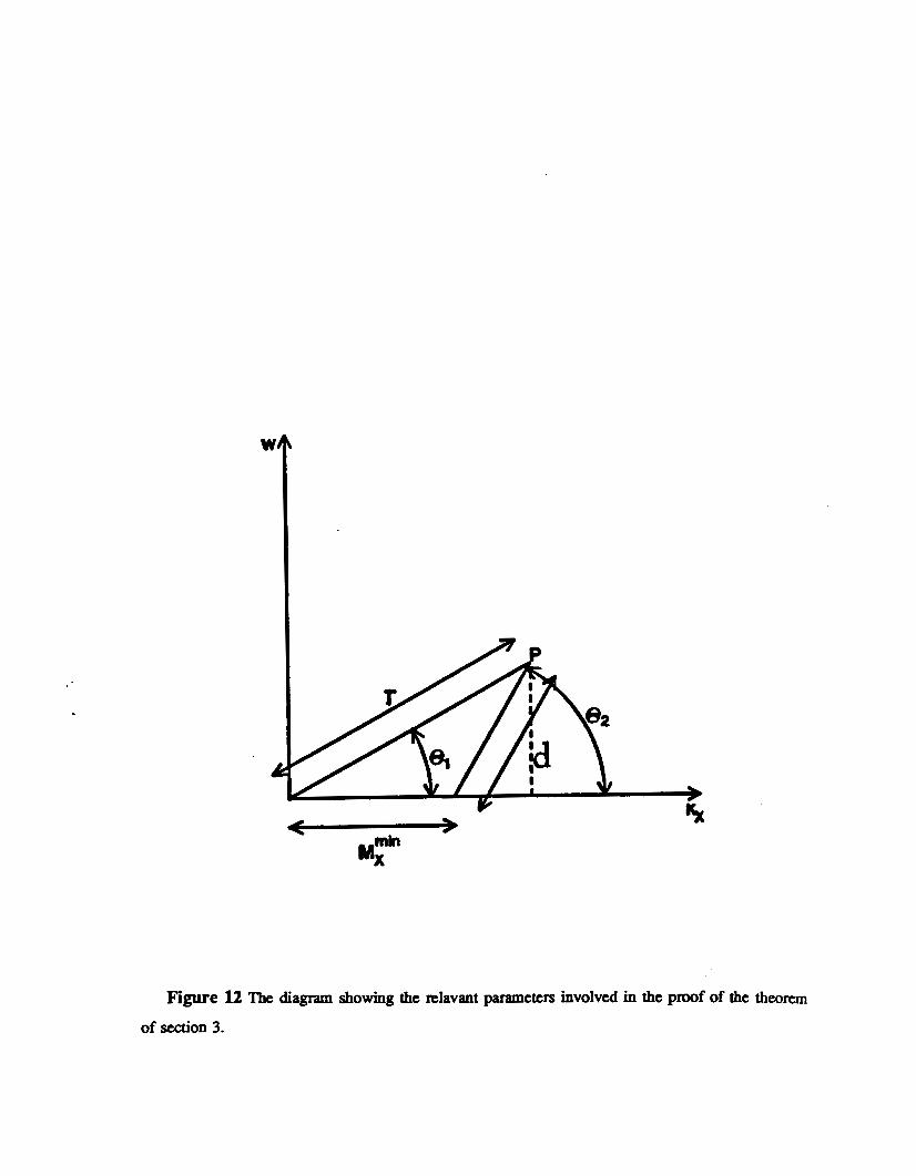
We can observe, from Figure 11 (or Figun 12), that there exists a point P, in the (r@) plane,
where the adjacent pattcms, cOrrtSpOnding to replicas of a (one-dimcnsional) cone, interstct without
overlapping. This point is the solution to the following equations
By substituting d, given by (3.19), into (3.18) we get
or
(3.18)
(3.19)
(3.20)
Expanding the sine and tangeat in (3.21) wc get the following expression
which, after some algebra leads to
2r sin(A4/2)- M y = tan8 + tan(A8/2) ’ (3.22)

20
This concludes the proof.
The thtorem shows us that the minimum interval, in the fiquency domain, between adjacent
sampling points (on the Ax axis) is bound, nonlinearly, by the de- of motion uncertainty. Conse-
quently, the spatial sampling rate px cannot be arbitrarily increased, but depends on the amount of
motion uncertainty. Since the spatial sampling rate px is the inverse of iUx (px = k), and Mz is bound, by motion uncertainty, to a minimum value e, px has a maximum value equal to c. If
px > p, we have aliasing of adjacent patterns (cones).
4 Conclusion
The extraction of optic flow, via space-time filming, is given in terms of a collection of filters which
are tuned to different orientations in space-time. The space-time Gabor and Cascades of the CS or
DOG filters ae specially suited for this task because they amstitutc (space-time) oriented filters. 1
show that it is possible, in particular, to use the cascaded filter approach of Fleet and Jepson [9] as an
energy filter, given that the exponential temporal part of the CS filter is substituted by a (temporal)
gaussian.
The space-time filtering approach to the extraction of optical flow is implemented on a sequence
of images which are closely displaced in time. The temporal interval bctwexm suctssive images in this
sequence corresponds to the (temporal) sampling rate, which as we saw before, is not independent of
the spatial sampling rate. In general, we want to use the sequence of images in such a way that we
are still able to extract the optical flow, but using the minimum number of images. This means that
we have to increase the temporal sampliig ratio as much as possible, without getting any aliasing
effect. As a collscqufncf of this, we have to ask ourselves what is the upper b i t for the temporal
4 CONCLUSION 21
(spatial) sampling rate such that:
1. We still are able to use a filtering approach to extract the optical flow
2. We do not get any aliasing effect.
As shown by the theorem of the previous Section, for Uniformly translating pattern, the maximum
spatial sampling interval is determined by the de- of motion uncertainty. The same can be shown
for the case of temporal sampling. If we sample at a lower rate than the minimum amount established
by the theorem of &on 3, we get aliasing. This answers the second part of the question.
The first part of the question is more difficult to be answered. Just as an illustration, we can
mention a problem which bcars similarities to the use of a filtering or feature matching approaches to
the extraction of optical flow. It is the hypothesis of the existence of two, distinct, proctssts to detect
or extract optic flow in humans [18,19], called short and long range processes. They arc studied, in
psychophysics, as a phtnommon of apparent motion, which is the capability of the human visual
systcm to be able to hterpolate the (spatial) position of moving objects between discrete presentations
of sucessive snapshots of the motion. We can establish a general nlationship bctwtcn short-range
and the filtering approach to optical flow, and between long-range and the ftaturt matching approach.
The short-range process opcratcs in short temporal mtervals (between sucessive m e s - also called
inter-stimulus interval S I , rauging fiwn 50 and 1oomS) and angular intervals of 15’ or less. The
long-range proctss, 011 the ather hand, can rake place even for IS1 as long as 400 ms [l J, and it works
mainly through the matching of features (edges, blobs, etc.), thus operating through the identification
of elements in sucessive frames.
If short and lang-range proccssts in humans ~IE really independent and operate through diffetent
mechanisms, it can point out to the possibility that if the filtering and ftaturt matching approaches
should bear some rcscmblanct with them, then there should exist a definite borderhe between both
approaches. In this sense we can say that (space-time) aliasing is one criteria by which we can decide
upon this problem.

4 CONCLUSION
Acknowledgment
22
I would like to thank A. Elfa, T. Kana&, L. Matthies and J. M o m for important discussions.
REFERENCES
References
23
[l] S. Ullman, The Interpretation of Visual Motion, 1979, M.I.T. Press, Cambridge, Massachusetts.
[2] B. K. P. Horn and B. G. Schunk, Dctennining Optical Flow, 1981, Artijiciclr InteUigence, 17,
185.
[3] E. C. Hitdreth, Computations Underlying the Measurement of V i a l Motion, 1984, Artificial
Intelligence, 23,309.
[4] B. E Buxton and H. Buxton, Computation of optic flow from the motion of edge features in
image squcnces, 1985, Image and Virion Computing. 2, No 2,59.
(51 D. J. Hecger, Optical Flow Using Spatiotemporal Filttrs, 1987, to appear in the International
Journal of Computtr Vision.
[6] E. H. Adelson and J. R Bergen, Spatiotemporal Energy Models for the Perception of Motion,
1985, Journal of the Optical Society of America A , 2 (22), 284.
[7] A. B. Watson and A. J. Ahumada, A Look at Motion in the Frequency Domain, 1983, Technical
Report 84352, NASA-Ames Research Center, and Model of Human Visual-Motion Sensing,
1985, Journal of the Optical Society of America A , 2 (22), 322.
[8] R C. Bolles and H.H. Baker, Epipolar-Plane Image Analysis: A Technique for Analysing
Motion Sequences, 1985, Proceedings: DARPA Image Understanding Worhhop, Miami Beach,
Florida 137.
(91 D. J. Fleet and A. D. Jepsan, On the Hierarchical Construction of Orientation and Velocity
Selective Wlters, 1985, University of Toronto Technical Repon RBCV-TR-85-8.
[lo] D. J. Fleet and A. D. Jepsm, Spatiotemporal Inseparability in Early Viion: centre-mund
Models and Velocity Selectivity, 1985, Compur. Intell. I , 89.
[ll] R S. Jasinschi, in preparation.
1121 W. McC. Siebert, Circuitr, Signals, and System, MIT Press.

REFERENCES 24
[13] C. E. Shannon, Communication in the Prtsence of Noise. January 1949. Proceedings of the
IR.E., IO.
[ 141 E H. C. Crick, D. C. M ~ I T and T. Poggio, An Information procesSing Approach to Understanding
the Visual Cortex, 1980, Artfcial Intelligence L&oratory of M.I.T. Memo No. 557.
[15] M. Fahle and T. Poggio, Visual Hyperacuity: Spatiotemporal Interpolation in Human Vision,
1981, Proc. R. SOC. London. B 213,451.
[la] L. H. Matthies, R S. Szcliski and T. Kanade, Kalman Filter-based Algorithms for Estimating
Depth from Image Sequences, 1987, Computer Science Department (CMU) technical report
CMU-CS-87- 185.
[17] N. M. Grzywacs and A. L. Yuille, Massively Parallel Implementations of Theories for Ap-
parent Motion, 1987, Artijicial Intelligence Laboratory and Center for Biological Information
Processing - MlT, A l . Memo No 888 and CBIP. Memo No 016
[ 181 0. J. Bmddick, Low-level and High-level Proctsses in Apparent Motion, 1980, Phil. Trans. R.
Soc. b n d . B 290,137.
[ 191 S. M. Anstis, The Perception of Apparent Motion Movement, 1980, Phyl. Tram. R. SOC. London
290,153.

Figure 1 One-layer cascade of space-time DOG filter with & = 0.77.(,, = 0, t = 2.83.


Figure 3 Fourier transform of the one-layer cascade of space-time DOG filter with & = 0.77,
= 0, T = 2.89.

..
Figure 4 Fourier transform of the one-layer cascade of space-time DOG filter with & = 0.52,
6 = 0, t = 1.93.

Figure 5 Twdayer cascade of space-time DOG filter with = 0.52, (’ = 0, r1 = 1.93,
.fi = 1.04, .f; = 0, 9 = 3.86.

Figure 6 Fourier tnrnsfom of the one-layer cascade of space-time DOG filter with 6: = 0.52,
,$ = 0, T~ = 1.93, = 1.04, i$ = 0, ;L = 3.86.
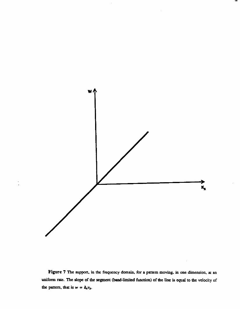
Figure 7 The support, in the frequency domain, for a pattern moving, in one dimension, at an
uniform rate. The slope of the segment (band-limited function) of the line is qual to the velocity of
thc pattern, that is w = &v,.

W
Figure 8 The sampled version of the support of an uniformly traaslating pattern, as rcprtsented
by Figure 7. The sampling interval is equal Mx.

Figure 9 The support, in the fmpency domain, of an uniformly translating pattern whose velocity
is measured with a certain uncertainty. The ape- of this cone is equal to this uncertainty.

Figure 10 Thc sampled version of the support xeprescmd in Figun 9. 'Ihc sampling interval
Mx is such that the adjacent cones don't overiap.

Figure ll The sampled version of Figure 9 in the case when the sampling rate is such that
is the the adjacent cants touch each other, but without overlapping. "he sampling rate Mx =
rntmlmal one such that then doesn't occur aliasing. . .
W
A
Figure 12 The diagram showing the relavant parameters involved in the p m f of the theorem
of d o n 3.
Recommended