Climate 2014, 2, 206-222; doi:10.3390/cli2030206
climate ISSN 2225-1154
www.mdpi.com/journal/climate
Article
Spatial-Temporal Variation and Prediction of Rainfall in Northeastern Nigeria
Umar M. Bibi 1,2,*, Jörg Kaduk 2,† and Heiko Balzter 2,†
1 Department of Geography, Adamawa State University Mubi, PMB 25 Mubi, Nigeria 2 Centre for Climate and Landscape Research, Department of Geography, University of Leicester,
Leicester LE1 7RH, UK; E-Mails: [email protected] (U.M.B); [email protected] (K.J.); [email protected] (H.B.)
† These authors contributed equally to this work.
* Author to whom correspondence should be addressed; E-Mail: [email protected] or
[email protected]; Tel.: +234-903-250-0833.
Received: 17 April 2014; in revised form: 1 September 2014 / Accepted: 3 September 2014 /
Published: 17 September 2014
Abstract: In Northeastern Nigeria seasonal rainfall is critical for the availability of water
for domestic use through surface and sub-surface recharge and agricultural production,
which is mostly rain fed. Variability in rainfall over the last 60 years is the main cause
for crop failure and water scarcity in the region, particularly, due to late onset of rainfall,
short dry spells and multi-annual droughts. In this study, we analyze 27 years (1980–2006)
of gridded daily rainfall data obtained from a merged dataset by the National Centre for
Environmental Prediction and Climate Research Unit reanalysis data (NCEP-CRU) for
spatial-temporal variability of monthly amounts and frequency in rainfall and rainfall
trends. Temporal variability was assessed using the percentage coefficient of variation
and temporal trends in rainfall were assessed using maps of linear regression slopes for
the months of May through October. These six months cover the period of the onset and
cessation of the wet season throughout the region. Monthly rainfall amount and frequency
were then predicted over a 24-month period using the Auto Regressive Integrated Moving
Average (ARIMA) Model. The predictions were evaluated using NCEP-CRU data for the
same period. Kolmogorov Smirnov test results suggest that despite there are some months
during the wet season (May–October) when there is no significant agreement (p < 0.05)
between the monthly distribution of the values of the model and the corresponding
24-month NCEP-CRU data, the model did better than simply replicating the long term
mean of the data used for the prediction. Overall, the model does well in areas and months
OPEN ACCESS
Climate 2014, 2 207
with lower temporal rainfall variability. Maps of the coefficient of variation and regression
slopes are presented to indicate areas of high rainfall variability and water deficit over the
period under study. The implications of these results for future policies on Agriculture and
Water Management in the region are highlighted.
Keywords: rainfall; spatial-temporal variability; ARIMA model; North-eastern Nigeria;
water scarcity
1. Introduction
In the semi-arid region of Northeastern Nigeria, seasonal rainfall patterns are very important
for continuous supply of water for domestic use, because rainfall leads to surface and sub-surface
recharge, and for rain-fed agricultural production [1–3]. Variability in rainfall over the last 60 years
has included repeatedly late onset of rainfall, short dry spells, and sometimes droughts lasting several
years. These events are the main factors determining crop failure and water scarcity in the region.
Large inter-annual variations in rainfall amounts and prolonged periods of droughts have been
recorded in 1967–1973 and 1983–1987 [4] with a negative impact on the region’s agricultural output
and severe consequences for the socio-economic situation of the people [5].
Rainfall in Northeastern Nigeria is controlled by the West African Monsoon (WAM) [6], and each
year, during the boreal summer, this air mass dominates the region in response to a low pressure belt
developing in North Africa with a parallel high pressure belt existing off the Gulf of Guinea. Once the
monsoon has commenced, rainfall events are mostly a product of instability and convection cells
developing in the lower atmosphere influenced by the nature and characteristics of the land surface [3].
The amount and frequency of rainfall in Nigeria generally increases from southwest to northeast
with some variations over short distances [7]. In the southernmost part of the region, the wet season
commences in late April, while the onset date of rains is delayed northwards with rainfall commencing
in July in the northernmost part.
A combination of different factors is believed to be responsible for recent climatic anomalies and
the seasonal and inter-annual variability of rainfall in the region. They include: regional and global sea
surface temperature (SST) changes [8,9], the depth and strength of the seasonal WAM winds [6], the
propagation of the African Easterly Jet (AEJ) [10,11] Saharan/Sahel aerosol dust concentrations [12,13],
and bio-geophysical feedback mechanisms [14–18]. Authors in [19] associated these changes to
global warming caused by anthropogenic emission of greenhouse gasses and the gradual expansion of
the tropics.
Several studies have analyzed rainfall trends and characteristics in Northeastern Nigeria.
Authors in [1,4] identified a negative trend in yearly rainfall totals in the region from 1961–1990 with
an increase in dry spells (dry episodes) during the wet season. They found a reduction of 8 mm·yr−1
over the period. Authors in [20] analyzed total annual rainfall, rainfall intensity, number of rain days,
onset and cessation of the wet season in six locations in the region over a 65 years period (1931–1996).
Their studies suggest a significant decrease in the annual rainfall from 1965 onwards mainly caused by
a reduction of high intensity rainfall of 25 mm or more per day at the peak of the wet season in the
Climate 2014, 2 208
months of August and September. There was a sign of a recovery [21] and a significant increase in
annual rainfalls in the 1990s compared to previous decades [22], but annual rainfall means were only
slightly above the long term mean [3].
There is a relationship between seasonal rainfall regimes and the availability of surface and ground
water resources in the region. Reference [2] pointed out that surface and ground water sources in the
semi-arid region of Northeastern Nigeria can be very depleted during the period, signaling the onset of
the wet season. Therefore, delays in the commencement of the wet season could cause serious
water shortages.
Several rainfall indices are used in planning for agricultural and water resources management [20];
of those monthly rainfall and number of rain days in a month are analyzed here because the two can
provide an insight in the variability of dry spells for each month during the wet season at inter-annual
and multi-decadal time scales.
In this paper, these variations are analyzed in a spatially distributed data set, i.e., for each grid
cell of a latitude/longitude grid. An understanding of the magnitude of the temporal scale of rainfall
anomalies will contribute to better planning for adaptation to water shortages, timing of planting crops,
and the nature and variety of crops to be cultivated. Short-term climate forecasting was used in this
study for the same reason. Reference [3] used spatially averaged time series data of the southern
sub-humid and northern semi-arid parts of the region to predict monthly rainfall and number of rain
days in a month. Similarly, in this study we used an ARIMA model to make the same predictions
spatially explicitly for each ½ degree pixel. The performance of the model in predicting monthly
rainfall and number of rain days (days with ≥1 mm rainfall) in a month is also presented and analyzed
in spatially distributed form.
The main objective of the study is to evaluate the temporal variation and trends in monthly rainfall
and number of rain days in a month for six months (May–October) over a 27-year period. Most of this
six-month period (May–October) is in the wet season in the region under the influence of the WAM.
The study also aimed to contribute to the study of ARIMA time series prediction models for
monthly rainfall prediction and evaluates the model performance in an area of transition between the
tropical sub-humid and semi-arid regions.
The data and methods used in the study are presented in the next section. Subsequently the results,
discussion and conclusions are presented in later sections.
2. Data and Methods
2.1. Data
The analysis presented here is based on the globally gridded 0.5° × 0.5° NCEP-CRU data version 3 [23]
for the period 1980–2006. These data are the six hourly National Centre for Environmental Prediction
(NCEP) reanalysis interpolated to 0.5° × 0.5° and scaled with the monthly precipitation, cloudiness,
relative humidity and temperature data from the Climate Research Unit (CRU) TS.3.1 0.5° × 0.5°
gridded monthly climatology. CRU TS3.1 only provides monthly means, but as we are here interested
in the number of rain days at least a daily product is required. We limited ourselves to the time period
1980–2006 because, before the 1980s, the original data sets are less reliable. Shortcomings of these data
Climate 2014, 2 209
sets and methods of interpolation were discussed by [24,25]. Data of Northeastern Nigeria were extracted
from the NCEP-CRU data set. The extracted data were aggregated to daily and subsequently monthly
rainfall considering only days with rainfall ≥ 1 mm [26,27]. A day with ≥1 mm rainfall was also
counted as a rain day and the monthly number of rain days was derived from this data set.
2.2. Analysis Methods
The two data sets of monthly rainfall and number of rain days of the study area were analyzed for
the magnitude of temporal variation using the percentage coefficient of variation (Equation (1)) and
linear regression slopes (Equation (2)) were used for evaluating temporal trends over the 27-year
period. These and other analyses were carried out at grid scale. Both analyses were carried out for the
months of May to October (i.e., May 1980, May 1981, …, May 2006) since these months cover the
wet season in the study area. Little or no rainfall is experienced in the rest of the months in most parts
of the study area. % = σμ × 100 (1)
where % is the coefficient of variation in percentage, σ is standard deviation, and μ is the mean.
Trends in monthly rainfall and the number of rain days for each month in the wet season
(May–October) over the 27-year (1980–2005) period was analyzed using slopes of linear regression
lines as given below: = + (2)
where is the regression line value at time or year n (n = 1, …, 27), is the intercept, and is the
slope of the regression line. Linear regression is a robust method of studying trends and has been used
previously for studying changes in vegetation over West Africa [28,29]. This was carried out monthly
at grid scale.
The ARIMA (auto-regressive integrated moving average) Model was used in this study for
predicting the years 2005 and 2006 (January 2005 to December 2006) from the 25 years 1980–2004
NCEP-CRU data.
The ARIMA model is a stochastic model used in time series prediction and has been used in the
fields of finance, hydrology, and climate forecasting. The ARIMA model is defined by [30]: ∅( )Φ( )( − ) = + θ( )Θ( ) (3)= (1 − ) (1 − ) (4)
where,
= white noise
= backward shift operator
= constant term
= order of the non-seasonal differencing operator
= order of the seasonal differencing operator
= seasonal length
= discrete time series value at time i
Climate 2014, 2 210
= stationary series formed by differencing the
= transformation of the series μ = mean level of the series ∅( ) = non-seasonal AR operator of order p θ( )= non-seasonal MA operator of order q Φ( ) = seasonal AR parameter of order P Θ( ) = seasonal MA parameter of order Q
= and either can be used depending on the non-stationarity of the time series
The ARIMA (p, d, q) model is made up of the Autoregressive (p), Integrated (d) and Moving
Average (q) components each represented by a non-negative integer. The autoregressive component
(p) predicts future values of a time series based on the weighted sum of the product of past values with
a regression coefficient and residual term. The moving average component (q) uses the mean of past
values to make prediction and then makes adjustments to the prediction based on previous forecast
errors. The p and q components produce a time dependent forecast even after removing non-stationarity.
The d component of the ARIMA model uses differencing to remove non-stationarity in the prediction.
The ARIMA process includes identifying the best p, d, q combination that fits a time series and
removes non-stationarity. This combination can be used to make forecasts. A diagnostic check can be
carried out to determine the performance of the model. In this study, the ARIMA (1, 2, 1) model was
identified as the best model that removes non-stationarity in the time series data used and was
therefore, adopted for making predictions.
Predictions using the suitable ARIMA model earlier identified were carried out using monthly data
in chronological order at grid level (i.e., ½° × ½° grid cell).
The Bland-Altman method was used to determine the degree of agreement [31,32] between
the values of the prediction (January 2005 to December 2006) and the corresponding 24-month
NCEP-CRU data set. This technique produces a scatter plot of the averages between two data sets
against their differences. This technique was carried at monthly level using spatially aggregated data
for the six wet months (May–October) by selecting corresponding months in each year (i.e., May 2005
and 2006). The approach is aimed at quantifying the agreement between two measurements (and in
this case observed and prediction) rather than testing for the association which is what happens in a
correlation test [31]. The difference (bias) is simply calculated by subtracting the values of the
reference data (or the independent variable x) from the values of the prediction (or the dependent variable y). The bias is plotted in the y-axis against the average of x and y (
) in the x-axis. The plot
has four horizontal lines. In the middle are the zero line and the mean difference line. The last two
horizontal lines mark the top and bottom limit of the agreement between x and y and it is expected
that 95% of all differences lie between these two lines. The lines are calculated as 2 × σ (standard
deviation) or more precisely 1.96 × σ. The limit of agreement show how spread apart the individual
differences from the mean bias. In the Bland-Altman plot, if the values of the bias are close to middle,
it signifies similarities in the values of the prediction and the further away the values of the bias the
larger the difference between x and y. Other than showing the limit of the agreement there is no cut off
point (or value) for the agreement and this is left for individual judgement. The Bland Altman plot is
widely used in various fields of clinical measurement and widely popularised by Bland and Altman [33].
Climate 2014, 2 211
In addition to the Bland-Altman method of studying the relationship between prediction and
actual data box plots were used to compare the percentiles and variability in the values of monthly
rainfall amounts and frequency for the prediction, corresponding NCEP-CRU data and the 25-year
NCEP-CRU data used in making the prediction. Spatially aggregated monthly data for the whole area
were used for both the Bland-Altman and box plots.
Whether the ARIMA prediction has some skill, i.e., whether it provides a better prediction than a
prediction based entirely on climatology – the simple repetition of the long term mean of the monthly
NCEP-CRU data – was explored with two approaches:
(1) The root mean square error ( ) was used to compare the prediction from the ARIMA
model and the long-term mean to the monthly NCEP-CRU data. It was calculated using the
following equation:
= ∑ ( − ) (5)
where, is the length of NCEP-CRU data, are the NCEP-CRU data for months and is the
rainfall prediction at month .
In any case when there is no significant goodness of fit (agreement) between the prediction and the
data used for the prediction a forecast skill was used to determine whether the model was better than
simply repeating the long term mean of the data. Forecast skill values greater than zero suggest a better
performance of the prediction than repeating the long term mean, values less than zero suggest an
under performance of the prediction and values of zero were regarded as the prediction repeating the
long term mean. The equation for the forecast skill is given below: ( ) = 1 − (6)
where is the mean square error of the prediction, and is the mean square error of
the reference NCEP-CRU data = ∑ ( − ) (7)
where is the mean square error, in this case is the 24-month prediction when calculating the or the long term mean when calculating , and is the 24-month (NCEP-CRU)
referral data.
The forecast skill was calculated using monthly data at grid scale.
(2) Furthermore, the 24-month prediction and the monthly means of the long term data
(1980–2004 NCEP-CRU data set) used in making the prediction doubled up to 24 months were
normalized using the mean standard deviates. The equation used in normalizing the data sets is
given below: = − μσ (8)
where, is the standard score of , is the data/prediction for month i, is the long term mean
for months i (e.g., August 2005, August 2006), and is the standard deviation for the months i.
Climate 2014, 2 212
The standard scores for each of the 24 months prediction and the standard scores of the long term
means were subjected to a Student’s t-test to determine whether they have the same mean. This was
carried for monthly data at grid level.
The R graphics (R studio 0.98.501) statistical and analytical software was used to calculate the
difference between the mean of the prediction and NCEP-CRU. The Kolmogorov Smirnov test was
used to test for the significance of the difference between the monthly distribution of the 24 months
(January 2005 to December 2006) prediction and the corresponding NCEP-CRU data. A null
hypothesis was set that there is no significant difference (or there is significant agreement) between the
prediction and the reference data. This hypothesis will be rejected if p < 0.05.
3. Results
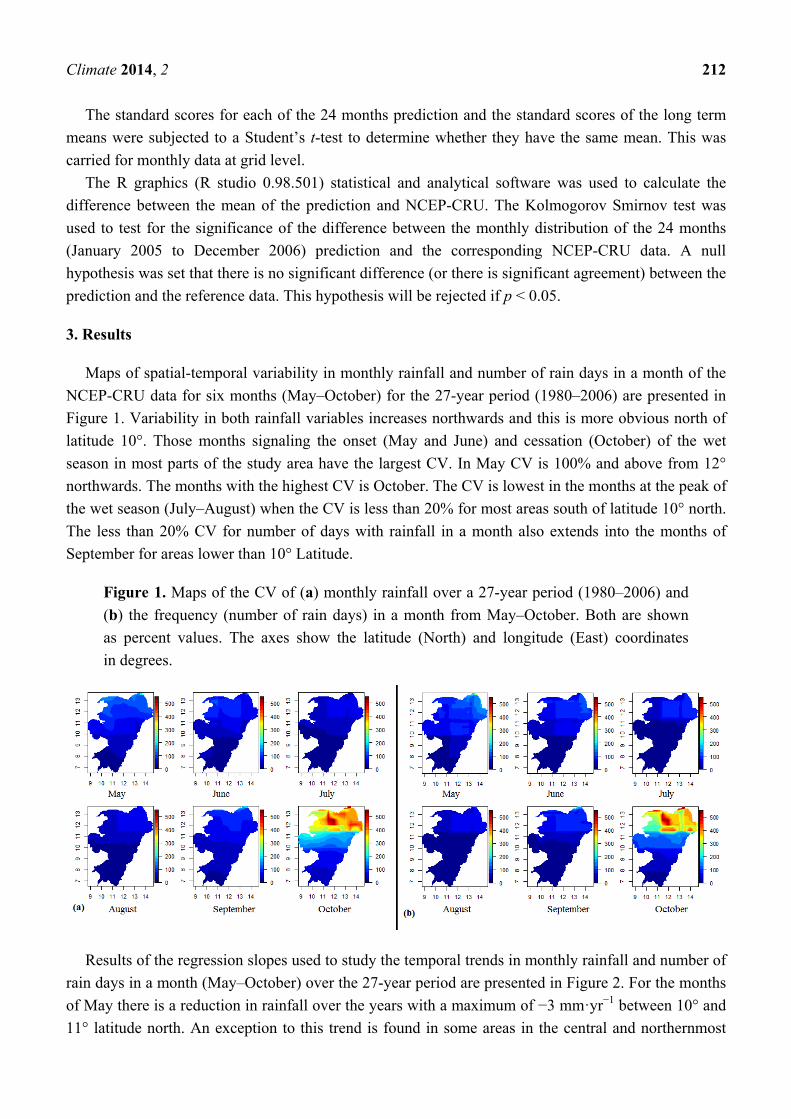
Maps of spatial-temporal variability in monthly rainfall and number of rain days in a month of the
NCEP-CRU data for six months (May–October) for the 27-year period (1980–2006) are presented in
Figure 1. Variability in both rainfall variables increases northwards and this is more obvious north of
latitude 10°. Those months signaling the onset (May and June) and cessation (October) of the wet
season in most parts of the study area have the largest CV. In May CV is 100% and above from 12°
northwards. The months with the highest CV is October. The CV is lowest in the months at the peak of
the wet season (July–August) when the CV is less than 20% for most areas south of latitude 10° north.
The less than 20% CV for number of days with rainfall in a month also extends into the months of
September for areas lower than 10° Latitude.
Figure 1. Maps of the CV of (a) monthly rainfall over a 27-year period (1980–2006) and
(b) the frequency (number of rain days) in a month from May–October. Both are shown
as percent values. The axes show the latitude (North) and longitude (East) coordinates
in degrees.
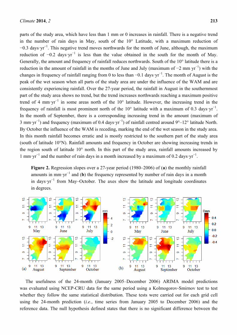
Results of the regression slopes used to study the temporal trends in monthly rainfall and number of
rain days in a month (May–October) over the 27-year period are presented in Figure 2. For the months
of May there is a reduction in rainfall over the years with a maximum of −3 mm·yr−1 between 10° and
11° latitude north. An exception to this trend is found in some areas in the central and northernmost
Climate 2014, 2 213
parts of the study area, which have less than 1 mm or 0 increases in rainfall. There is a negative trend
in the number of rain days in May, south of the 10° Latitude, with a maximum reduction of
−0.3 days·yr−1. This negative trend moves northwards for the month of June, although, the maximum
reduction of −0.2 days·yr−1 is less than the value obtained in the south for the month of May.
Generally, the amount and frequency of rainfall reduces northwards. South of the 10° latitude there is a
reduction in the amount of rainfall in the months of June and July (maximum of −2 mm yr−1) with the
changes in frequency of rainfall ranging from 0 to less than −0.1 days·yr−1. The month of August is the
peak of the wet season when all parts of the study area are under the influence of the WAM and are
consistently experiencing rainfall. Over the 27-year period, the rainfall in August in the southernmost
part of the study area shows no trend, but the trend increases northwards reaching a maximum positive
trend of 4 mm·yr−1 in some areas north of the 10° latitude. However, the increasing trend in the
frequency of rainfall is most prominent north of the 10° latitude with a maximum of 0.3 days·yr−1.
In the month of September, there is a corresponding increasing trend in the amount (maximum of
3 mm·yr−1) and frequency (maximum of 0.4 days·yr−1) of rainfall centred around 9°–12° latitude North.
By October the influence of the WAM is receding, marking the end of the wet season in the study area.
In this month rainfall becomes erratic and is mostly restricted to the southern part of the study area
(south of latitude 10°N). Rainfall amounts and frequency in October are showing increasing trends in
the region south of latitude 10° north. In this part of the study area, rainfall amounts increased by
1 mm·yr−1 and the number of rain days in a month increased by a maximum of 0.2 days·yr−1.
Figure 2. Regression slopes over a 27-year period (1980–2006) of (a) the monthly rainfall
amounts in mm·yr−1 and (b) the frequency represented by number of rain days in a month
in days·yr−1 from May–October. The axes show the latitude and longitude coordinates
in degrees.
The usefulness of the 24-month (January 2005–December 2006) ARIMA model predictions
was evaluated using NCEP-CRU data for the same period using a Kolmogorov-Smirnov test to test
whether they follow the same statistical distribution. These tests were carried out for each grid cell
using the 24-month prediction (i.e., time series from January 2005 to December 2006) and the
reference data. The null hypothesis defined states that there is no significant difference between the
Climate 2014, 2 214
prediction and the NCEP-CRU data. If p < 0.05 the null hypothesis is rejected. The results of the
Kolmogorov Smirnov test p > 0.05 (not presented in the paper) was obtained in areas south of 9°
northern latitude and Lake Chad in the north, therefore, the null hypothesis was accepted that there is
no significant difference between the distribution of the values between the 24-month predictions and
the reference data. However, most parts of the study area especially north of latitude 9°N have
p < 0.05, and therefore, the null hypothesis was rejected for those areas. A similar result was obtained
for rainfall frequency. Following the same procedure tests were carried for selected months in the wet
season (May–October) with the significance of the agreement increasing for each months from July
reaching a peak in September (September 2005 and September 2006) where p > 0.05 was obtained for
most areas.
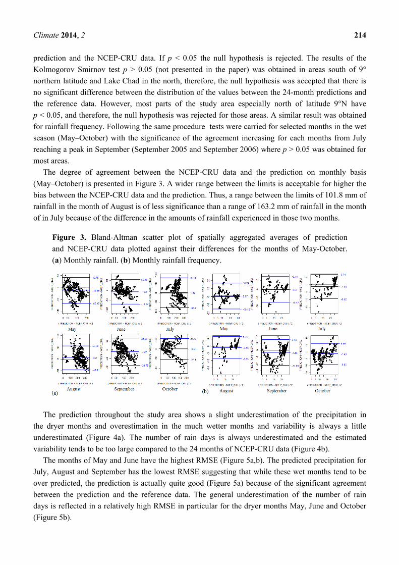
The degree of agreement between the NCEP-CRU data and the prediction on monthly basis
(May–October) is presented in Figure 3. A wider range between the limits is acceptable for higher the
bias between the NCEP-CRU data and the prediction. Thus, a range between the limits of 101.8 mm of
rainfall in the month of August is of less significance than a range of 163.2 mm of rainfall in the month
of in July because of the difference in the amounts of rainfall experienced in those two months.
Figure 3. Bland-Altman scatter plot of spatially aggregated averages of prediction
and NCEP-CRU data plotted against their differences for the months of May-October.
(a) Monthly rainfall. (b) Monthly rainfall frequency.
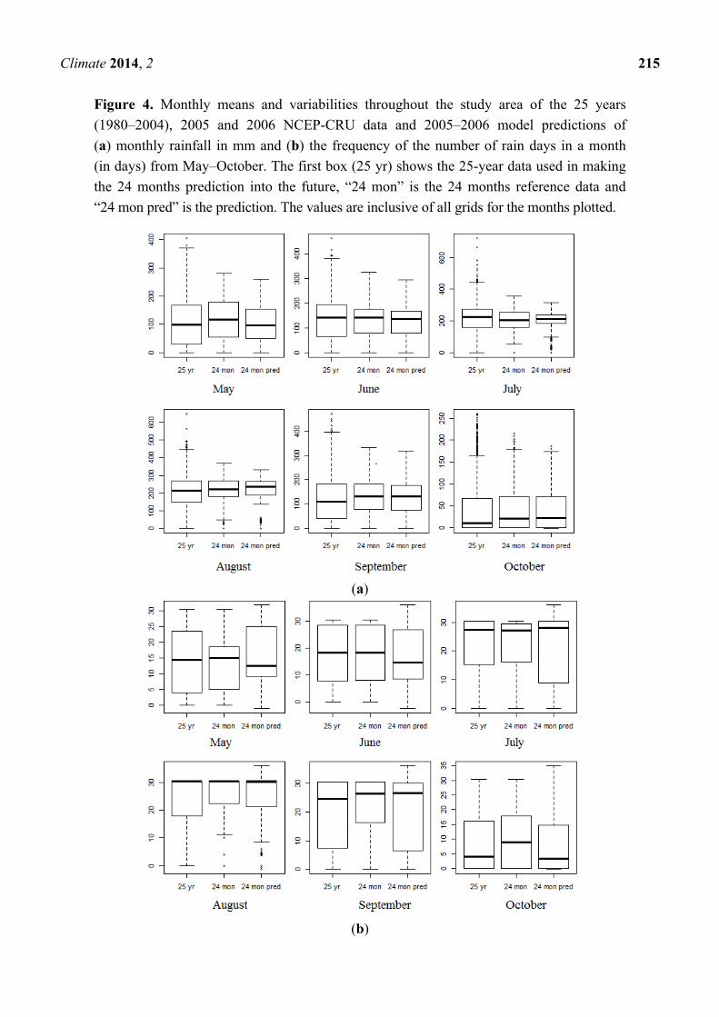
The prediction throughout the study area shows a slight underestimation of the precipitation in
the dryer months and overestimation in the much wetter months and variability is always a little
underestimated (Figure 4a). The number of rain days is always underestimated and the estimated
variability tends to be too large compared to the 24 months of NCEP-CRU data (Figure 4b).
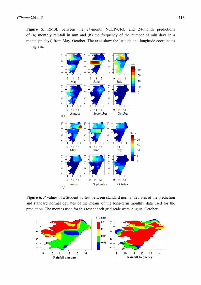
The months of May and June have the highest RMSE (Figure 5a,b). The predicted precipitation for
July, August and September has the lowest RMSE suggesting that while these wet months tend to be
over predicted, the prediction is actually quite good (Figure 5a) because of the significant agreement
between the prediction and the reference data. The general underestimation of the number of rain
days is reflected in a relatively high RMSE in particular for the dryer months May, June and October
(Figure 5b).
Climate 2014, 2 215
Figure 4. Monthly means and variabilities throughout the study area of the 25 years
(1980–2004), 2005 and 2006 NCEP-CRU data and 2005–2006 model predictions of
(a) monthly rainfall in mm and (b) the frequency of the number of rain days in a month
(in days) from May–October. The first box (25 yr) shows the 25-year data used in making
the 24 months prediction into the future, “24 mon” is the 24 months reference data and
“24 mon pred” is the prediction. The values are inclusive of all grids for the months plotted.
(a)
(b)
Climate 2014, 2 216
Figure 5. RMSE between the 24-month NCEP-CRU and 24-month predictions
of (a) monthly rainfall in mm and (b) the frequency of the number of rain days in a
month (in days) from May–October. The axes show the latitude and longitude coordinates
in degrees.
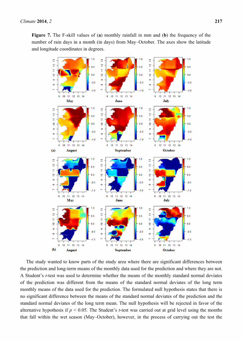
Figure 6. P-values of a Student’s t-test between standard normal deviates of the prediction
and standard normal deviates of the means of the long-term monthly data used for the
prediction. The months used for this test at each grid scale were August–October.
Climate 2014, 2 217
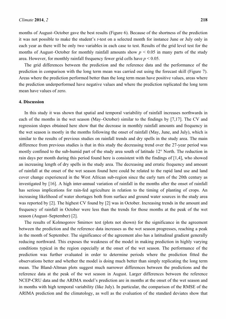
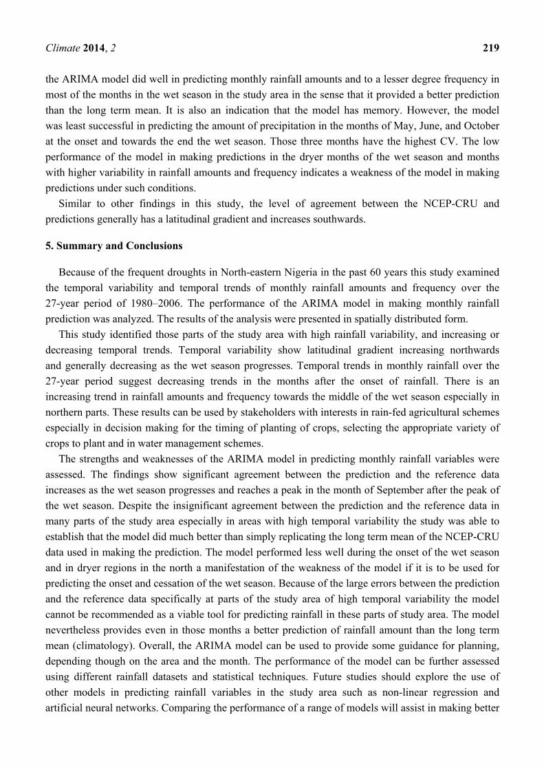
Figure 7. The F-skill values of (a) monthly rainfall in mm and (b) the frequency of the
number of rain days in a month (in days) from May–October. The axes show the latitude
and longitude coordinates in degrees.
The study wanted to know parts of the study area where there are significant differences between
the prediction and long-term means of the monthly data used for the prediction and where they are not.
A Student’s t-test was used to determine whether the means of the monthly standard normal deviates
of the prediction was different from the means of the standard normal deviates of the long term
monthly means of the data used for the prediction. The formulated null hypothesis states that there is
no significant difference between the means of the standard normal deviates of the prediction and the
standard normal deviates of the long term mean. The null hypothesis will be rejected in favor of the
alternative hypothesis if p < 0.05. The Student’s t-test was carried out at grid level using the months
that fall within the wet season (May–October), however, in the process of carrying out the test the
Climate 2014, 2 218
months of August–October gave the best results (Figure 6). Because of the shortness of the prediction
it was not possible to make the student’s t-test on a selected month for instance June or July only in
each year as there will be only two variables in each case to test. Results of the grid level test for the
months of August–October for monthly rainfall amounts show p < 0.05 in many parts of the study
area. However, for monthly rainfall frequency fewer grid cells have p < 0.05.
The grid differences between the prediction and the reference data and the performance of the
prediction in comparison with the long term mean was carried out using the forecast skill (Figure 7).
Areas where the prediction performed better than the long term mean have positive values, areas where
the prediction underperformed have negative values and where the prediction replicated the long term
mean have values of zero.
4. Discussion
In this study it was shown that spatial and temporal variability of rainfall increases northwards in
each of the months in the wet season (May–October) similar to the findings by [7,17]. The CV and
regression slopes obtained here show that the decrease in monthly rainfall amounts and frequency in
the wet season is mostly in the months following the onset of rainfall (May, June, and July), which is
similar to the results of previous studies on rainfall trends and dry spells in the study area. The main
difference from previous studies is that in this study the decreasing trend over the 27-year period was
mostly confined to the sub-humid part of the study area south of latitude 12° North. The reduction in
rain days per month during this period found here is consistent with the findings of [1,4], who showed
an increasing length of dry spells in the study area. The decreasing and erratic frequency and amount
of rainfall at the onset of the wet season found here could be related to the rapid land use and land
cover change experienced in the West African sub-region since the early turn of the 20th century as
investigated by [16]. A high inter-annual variation of rainfall in the months after the onset of rainfall
has serious implications for rain-fed agriculture in relation to the timing of planting of crops. An
increasing likelihood of water shortages both from surface and ground water sources in the study area
was reported by [2]. The highest CV found by [2] was in October. Increasing trends in the amount and
frequency of rainfall in October were less than the trends for those months at the peak of the wet
season (August–September) [2].
The results of Kolmogorov Smirnov test (plots not shown) for the significance in the agreement
between the prediction and the reference data increases as the wet season progresses, reaching a peak
in the month of September. The significance of the agreement also has a latitudinal gradient generally
reducing northward. This exposes the weakness of the model in making prediction in highly varying
conditions typical in the region especially at the onset of the wet season. The performance of the
prediction was further evaluated in order to determine periods where the prediction fitted the
observations better and whether the model is doing much better than simply replicating the long term
mean. The Bland-Altman plots suggest much narrower differences between the predictions and the
reference data at the peak of the wet season in August. Larger differences between the reference
NCEP-CRU data and the ARIMA model’s prediction are in months at the onset of the wet season and
in months with high temporal variability (like July). In particular, the comparison of the RMSE of the
ARIMA prediction and the climatology, as well as the evaluation of the standard deviates show that
Climate 2014, 2 219
the ARIMA model did well in predicting monthly rainfall amounts and to a lesser degree frequency in
most of the months in the wet season in the study area in the sense that it provided a better prediction
than the long term mean. It is also an indication that the model has memory. However, the model
was least successful in predicting the amount of precipitation in the months of May, June, and October
at the onset and towards the end the wet season. Those three months have the highest CV. The low
performance of the model in making predictions in the dryer months of the wet season and months
with higher variability in rainfall amounts and frequency indicates a weakness of the model in making
predictions under such conditions.
Similar to other findings in this study, the level of agreement between the NCEP-CRU and
predictions generally has a latitudinal gradient and increases southwards.
5. Summary and Conclusions
Because of the frequent droughts in North-eastern Nigeria in the past 60 years this study examined
the temporal variability and temporal trends of monthly rainfall amounts and frequency over the
27-year period of 1980–2006. The performance of the ARIMA model in making monthly rainfall
prediction was analyzed. The results of the analysis were presented in spatially distributed form.
This study identified those parts of the study area with high rainfall variability, and increasing or
decreasing temporal trends. Temporal variability show latitudinal gradient increasing northwards
and generally decreasing as the wet season progresses. Temporal trends in monthly rainfall over the
27-year period suggest decreasing trends in the months after the onset of rainfall. There is an
increasing trend in rainfall amounts and frequency towards the middle of the wet season especially in
northern parts. These results can be used by stakeholders with interests in rain-fed agricultural schemes
especially in decision making for the timing of planting of crops, selecting the appropriate variety of
crops to plant and in water management schemes.
The strengths and weaknesses of the ARIMA model in predicting monthly rainfall variables were
assessed. The findings show significant agreement between the prediction and the reference data
increases as the wet season progresses and reaches a peak in the month of September after the peak of
the wet season. Despite the insignificant agreement between the prediction and the reference data in
many parts of the study area especially in areas with high temporal variability the study was able to
establish that the model did much better than simply replicating the long term mean of the NCEP-CRU
data used in making the prediction. The model performed less well during the onset of the wet season
and in dryer regions in the north a manifestation of the weakness of the model if it is to be used for
predicting the onset and cessation of the wet season. Because of the large errors between the prediction
and the reference data specifically at parts of the study area of high temporal variability the model
cannot be recommended as a viable tool for predicting rainfall in these parts of study area. The model
nevertheless provides even in those months a better prediction of rainfall amount than the long term
mean (climatology). Overall, the ARIMA model can be used to provide some guidance for planning,
depending though on the area and the month. The performance of the model can be further assessed
using different rainfall datasets and statistical techniques. Future studies should explore the use of
other models in predicting rainfall variables in the study area such as non-linear regression and
artificial neural networks. Comparing the performance of a range of models will assist in making better
Climate 2014, 2 220
predictions to support decision-making and reducing losses in rain-fed agricultural production in the
study area.
Acknowledgments
The authors are grateful and wish to acknowledge the use of NCEP-CRU data received from
Nicolas Viovy. We are thankful to the two anonymous reviewers who made constructive comments on
how to improve on the paper.
Author Contributions
Umar M. Bibi conceived the research and processed all the data. Joerg Kaduk proposed and
provided the convenient climatological data for the analysis. Umar M. Bibi, Joerg Kaduk and
Heiko Balzter all contributed in designing the research, writing and editing the paper.
Conflicts of Interest
The authors declare no conflict of interest.
References
1. Hess, T.M.; Stephens, W.; Maryah, U.M. Rainfall trends in the North East Arid Zone of Nigeria
1961–1990. Agric. For. Meteorol. 1995, 74, 87–97.
2. Tarhule, A.; Woo, M.-K. Adaptations to the dynamics of rural water supply from natural sources:
A village example in semi-arid Nigeria. Mitig. Adapt. Strateg. Glob. Chang. 2002, 7, 215–237.
3. Bibi, U.M. The Impact of Climate Variability and Land Cover Change on Land Surface
Conditions in North-Eastern Nigeria. Ph.D. Thesis, University of Leicester, Leicester, UK, 2013.
4. Amissah-Arthur, A.; Jagtap, S.S. Geographic variation in growing season rainfall during three
decades in Nigeria using principal component and cluster analyses. Theor. Appl. Climatol. 1999,
63, 107–116.
5. Jalloh, A.; Roy-Macauley, H.; Sereme, P. Major agro-ecosystems of West and Central Africa:
Brief description, species richness, management, environmental limitations and concerns.
Agric. Ecosyst. Environ. 2012, 157, 5–16.
6. Lamb, P.J. West African water vapor variations between recent contrasting Subsaharan rainy
seasons. Tellus A 1983, 35A, 198–212.
7. Mortimore, M.; Adams, M.W. Working the Sahel: Environment and Society in Northern Nigeria;
Routledge Publishers: London, UK, 1999.
8. Lamb, P.J. Large-scale Tropical Atlantic surface circulation patterns associated with Subsaharan
weather anomalies. Tellus 1978, 30, 240–251.
9. Folland, C.K.; Palmer, T.N.; Parker, D.E. Sahel rainfall and worldwide sea temperatures, 1901–
85. Nature 1986, 320, 602–607.
10. Fontaine, B.; Janicot, S.; Moron, V. Rainfall anomaly patterns and wind field signals over West
Africa in August (1958–1989). J. Clim. 1995, 8, 1503–1510.
Climate 2014, 2 221
11. Cook, K.H. Generation of the African easterly jet and its role in determining West African
precipitation. J. Clim. 1999, 12, 1165–1184.
12. Carlson, T.N.; Prospero, J.M. The Large-Scale movement of Saharan air outbreaks over the
Northern Equatorial Atlantic. J. Appl. Meteorol. 1972, 11, 283–297.
13. Nicholson, S.E. The West African Sahel: A Review of recent studies on the rainfall regime and Its
interannual variability. ISRN Meteorol. 2013, 2013, doi:10.1155/2013/453521.
14. Charney, J.G. Dynamics of deserts and drought in the Sahel. Q. J. R. Meteorol. Soc. 1975, 101,
193–202.
15. Xue, Y.; Shukla, J. The influence of land surface properties on Sahel climate. Part 1:
Desertification. J. Clim. 1993, 6, 2232–2245.
16. Taylor, C.M.; Lambin, E.F.; Stephenne, N.; Harding, R.J.; Essery, R.L.H. The influence of land
use change on climate in the Sahel. J. Clim. 2002, 15, 3615–3629.
17. Oguntunde, P.G.; Abiodun, B.J.; Lischeid, G. Rainfall trends in Nigeria, 1901–2000. J. Hydrol.
2011, 411, 207–218.
18. Los, S.O.; Weedon, G.P.; North, P.R.J.; Kaduk, J.D.; Taylor, C.M.; Cox, P.M. An observation-based
estimate of the strength of rainfall-vegetation interactions in the Sahel. Geophys. Res. Lett. 2006,
33, L16402.
19. Lucas, C.; Timbal, B.; Nguyen, H. The expanding tropics: A critical assessment of the
observational and modeling studies. Wiley Interdiscip. Rev. Clim. Chang. 2014, 5, 89–112.
20. Tarhule, A.; Woo, M.-K. Changes in rainfall characteristics in northern Nigeria. Int. J. Climatol.
1998, 18, 1261–1271.
21. Nicholson, S.E.; Some, B.; Kone, B. An analysis of recent rainfall conditions in West Africa,
including the rainy seasons of the 1997 El Niño and the 1998 La Niña years. J. Clim. 2000, 13,
2628–2640.
22. Ati, O.F.; Stigter, C.J.; Iguisi, E.O.; Afolayan, J.O. Profile of rainfall change and variability in the
Northern Nigeria 1953–2002. Res. J. Environ. Earth Sci. 2009, 1, 58–63.
23. Viovy, N. Laboratoire des Sciences du Climat et de l’Environment, Gif-sur-Yvette, France,
Personal communication, 2011.
24. Mitchell, T.D.; Jones, P.D. An improved method of constructing a database of monthly climate
observations and associated high-resolution grids. Int. J. Climatol. 2005, 25, 693–712.
25. Mitchell, T.D.; Hulme, M. Predicting regional climate change: Living with uncertainty.
Prog. Phys. Geogr. 1999, 23, 57–78.
26. Odekunle, T.O. Determining rainy season onset and retreat over Nigeria from precipitation
amount and number of rainy days. Theor. Appl. Climatol. 2006, 83, 193–201.
27. Schmidli, J.; Frei, C. Trends of heavy precipitation and wet and dry spells in Switzerland during
the 20th century. Int. J. Climatol. 2005, 25, 753–771.
28. Eklundh, L.; Olsson, L. Vegetation index trends for the African Sahel 1982–1999. Geophys. Res.
Lett. 2003, 30, doi:10.1029/2002GL016772.
29. Anyamba, A.; Tucker, C.J.; Pak, E.W. Thirty-two years of Sahelian zone growing season
non-stationary NDVI3g patterns and trends. Remote Sens. 2014, 6, 3101–3122.
30. Yurekli, K.; Kurunc, A. Simulating agricultural drought periods based on daily rainfall and crop
water consumption. J. Arid Environ. 2006, 67, 629–640.

Climate 2014, 2 222
31. Bland, J.M.; Altman, D.G. Measuring agreement in method comparison studies. Stat. Methods
Med. Res. 1999, 8, 135–160.
32. Bland, J.M.; Altman, D.G. Applying the right statistics: Analyses of measurement studies.
Ultrasound Obstet. Gynecol. 2003, 22, 85–93.
33. Myles, P.S.; Cui, J.I. Using the Bland–Altman method to measure agreement with repeated
measures. Br. J. Anaesth. 2007, 99, 309–311.
© 2014 by the authors; licensee MDPI, Basel, Switzerland. This article is an open access article
distributed under the terms and conditions of the Creative Commons Attribution license
(http://creativecommons.org/licenses/by/3.0/).
Recommended