1
Speed Sensorless and MPPT Control of IPM
Synchronous Generator for Wind Energy
Conversion System
by
Nirav R. Patel
SUBMITTED IN PARTIAL FULFILLMENT OF THE
REQUIREMENTS FOR THE DEGREE OF
MASTER OF SCIENCE
AT
LAKEHEAD UNIVERSITY
THUNDER BAY, ONTARIO
May, 2013
©Copyright by Nirav R. Patel

II
Abstract
The popularity of renewable energy has experienced significant growth recently due to
the foreseeable exhaustion of conventional fossil fuel power generation methods and increasing
realization of the adverse effects that conventional fossil fuel power generation has on the
environment. Among the renewable energy sources, wind power generation is rapidly becoming
competitive with conventional fossil fuel sources. The wind turbines in the market have a variety
of innovative concepts, with proven technology for both generators and power electronics
interfaces. Recently, variable-speed permanent magnet synchronous generator (PMSG) based
wind energy conversion systems (WECS) is becoming more attractive in comparison to the
fixed-speed WECS. In the variable-speed generation system, the wind turbine can be operated at
maximum power operating points over a wide speed range by adjusting the shaft speed
optimally.
This thesis presents both wind and rotor speed sensorless control for the direct-drive interior
permanent magnet synchronous generator (IPMSG) with maximum power point tracking
(MPPT) algorithm. The proposed method, without requiring the knowledge of wind speed, air
density or turbine parameters, generates optimum speed command for speed control loop of
vector controlled machine side converter. The MPPT algorithm based on perturbation and
observation uses only estimated active power as its input to track peak output power points in
accordance with wind speed change and incorporates proposed sensorless control to transfer
maximum dc-link power from generator.

III
In this work for the IPMSG, the rotor position and speed are estimated based on model
reference adaptive system. Additionally, it incorporates flux weakening controller (FWC) for
wide operating speed range at various wind speed and other disturbances. Matlab/Simulink based
simulation model of the proposed sensorless MPPT control of IPMSG based WECS is built to
verify the effectiveness of the system. The MPPT controller has been tested for variable wind
speed conditions. The performance of the proposed WECS is also compared with the
conventional control of WECS system. The proposed IPMSG based WECS incorporating the
MPPT and sensorless algorithms is successfully implemented in real-time using the digital signal
processor (DSP) board DS1104 for a laboratory 5 hp machine. A 5 hp DC motor is used as wind
turbine to drive the IPMSG. The speed tracking performance and maximum power transfer
capability of the proposed WECS are verified by both simulation and experimental results at
different speed conditions.

IV
Acknowledgements
I would like to express my most sincere gratitude to God and those people who have
supported and helped me in the preparation of this thesis. Dr. M. N. Uddin, my thesis supervisor,
has been vital in the completion of this thesis and success of the project. It is due to his constant
inspiration and encouragement that I have gained a deeper understanding of engineering and
made progress toward solving problems and improving my skills as a researcher. This work
might not be possible without his guidance. I wish to thank my thesis committee members Dr.
Krishnamoorthy Natarajan and Dr. Dimiter Alexandrov. I acknowledge the support from
Lakehead University professors for their guidance to complete my thesis. I would like to give
many thanks to my fellow graduate students, especially Bhavin Patel for his guidance throughout
the last two years, and staff of Lakehead University.
Numerous people and innumerable instances, which I cannot enumerate in a single page,
have helped me to accomplish this project. Finally I’d like to express sincere appreciation to my
parents, Rukhiben and Rameshbhai Patel, and friends who have always been patient and
supportive to me. I would like to appreciate all the circumstances around me, which have been so
generous to this humble being.

V
Table of Contents
Table of Figures .................................................................................................................................... VII
List of Symbols ....................................................................................................................................... X
List of Acronyms .................................................................................................................................. XIII
Chapter 1 ................................................................................................................................................. 1
Introduction ......................................................................................................................................... 1
1.1 Research Motivation .................................................................................................................. 1
1.2 Literature Survey on WECS ....................................................................................................... 4
1.3 Objective of Thesis .................................................................................................................. 24
1.4 Thesis Organization ................................................................................................................. 25
Chapter 2 ............................................................................................................................................... 27
Modeling of Wind Energy Conversion System................................................................................... 27
2.1 General Overview of the Proposed WECS................................................................................ 27
2.2 Park's and Clarke's Transformations ......................................................................................... 28
2.3 Introduction to Permanent Magnet Synchronous Machines ....................................................... 33
2.4 Mathematical Model Development ........................................................................................... 36
2.5 Vector Control of IPMSM ........................................................................................................ 39
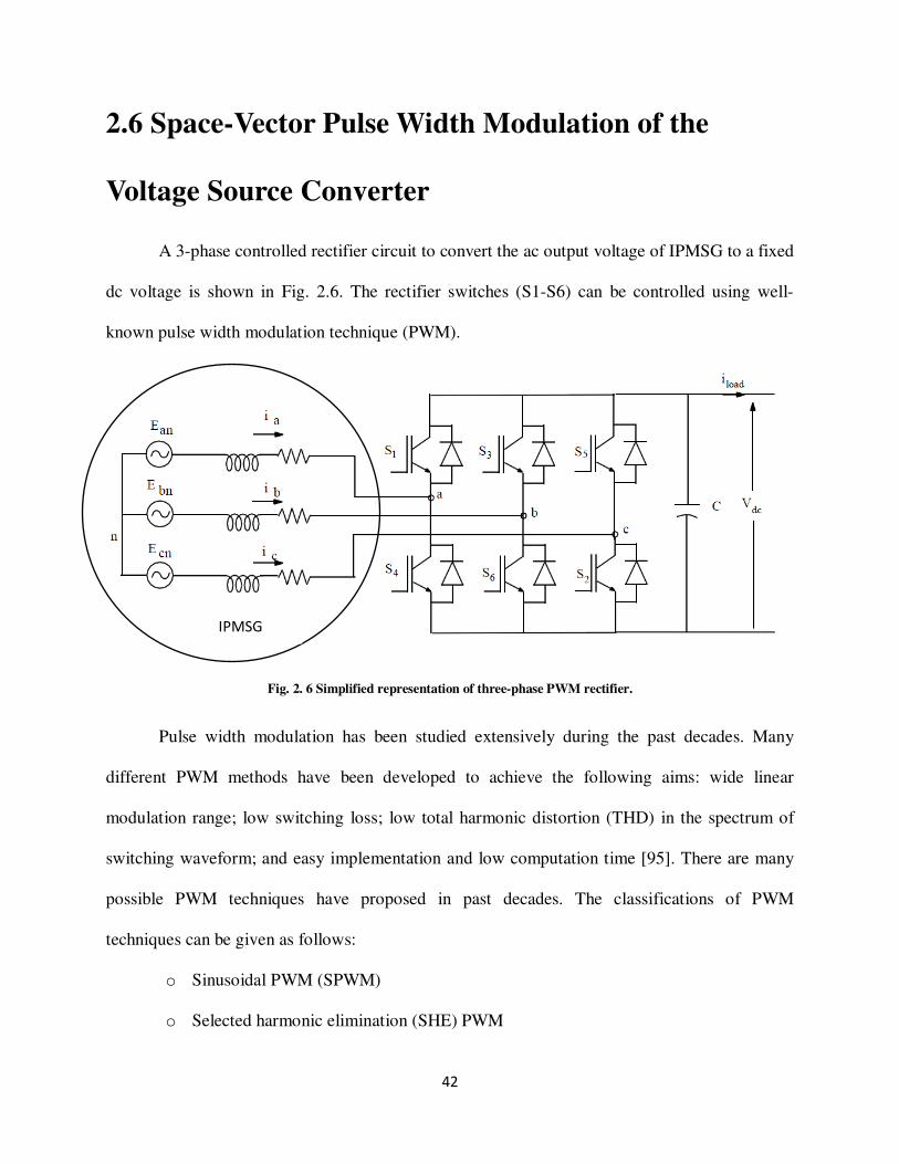
2.6 Space-Vector Pulse Width Modulation of the Voltage Source Converter .................................. 42
2.7 Concluding Remarks ................................................................................................................ 44
Chapter 3 ............................................................................................................................................... 45
Power Extraction Strategies and Control Techniques ......................................................................... 45
3.1 Conventional Control of WT .................................................................................................... 48
3.2 Proposed MPPT Algorithm ...................................................................................................... 50
3.3 Overall Control of the Proposed WECS System ....................................................................... 52
3.4 Flux Controller Design ............................................................................................................. 54
3.5 Simulation Results ................................................................................................................... 57
3.4 Concluding Remarks ................................................................................................................ 73
Chapter 4 ............................................................................................................................................... 74
Sensorless Control- Position and Speed Estimation ............................................................................ 74

VI
4.1 Introduction ............................................................................................................................. 74
4.2 Strategies for Position and Speed Estimation for IPMSM ......................................................... 75
4.2 Model Reference Adaptive System Based Speed Estimation .................................................... 77
4.3 Simulation Results ................................................................................................................... 80
4.4 Concluding Remarks ................................................................................................................ 84
Chapter 5 ............................................................................................................................................... 85
Real-time Implementation.................................................................................................................. 85
5.1 Introduction ............................................................................................................................. 85
5.2 Experimental Setup .................................................................................................................. 85
5.3 Experimental Results ............................................................................................................... 91
5.5 Concluding Remarks ................................................................................................................ 96
Chapter 6 ............................................................................................................................................... 97
Conclusions ....................................................................................................................................... 97
6.1 Concluding Remarks ................................................................................................................ 97
6.2 Future work ............................................................................................................................. 98
References............................................................................................................................................. 99
Appendix –A ....................................................................................................................................... 114
IPMSM Parameters ......................................................................................................................... 114
Appendix –B ....................................................................................................................................... 115
Simulink Blocks for Simulation ....................................................................................................... 116
Appendix C ......................................................................................................................................... 131
Drive and Interface Circuit ............................................................................................................... 131
Appendix D ......................................................................................................................................... 134
Real-Time Simulink Model ............................................................................................................. 134

VII
Table of Figures
Fig. 1. 1 Total installed wind power capacity (a) in 2010-2012 (MW) around the world (b) in 2010-2012
(MW) in different countries [9]. ............................................................................................................... 3
Fig. 1. 2 Power coefficient Cp as a function of the tip speed ratio λ and the pitch angle β. ....................... 7
Fig. 1. 3 Mechanical power (W) vs rotor speed (rpm). .............................................................................. 8
Fig. 1. 4 Wind speed vs variation of turbine power with wind speed. ....................................................... 8
Fig. 1. 5 WECS categories (a) fixed speed wind turbine with an asynchronous squirrel cage IG (b) variable
speed wind turbine with a DFIG (c) variable speed wind turbine using PMSG (d) brushless generator with
gear box. ............................................................................................................................................... 11
Fig. 1. 6 Wind turbine generator types. .................................................................................................. 11
Fig. 1. 7 Sketch of (a) a constant speed WT with gear box (b) direct drive WT [13]. ................................ 12
Fig. 1. 8 Wind turbine rotor types. ......................................................................................................... 14
Fig. 1. 9 Three bladed horizontal Axis wind turbine [9]. .......................................................................... 16
Fig. 1. 10 Darrieus wind turbine [8]. ....................................................................................................... 17
Fig. 1. 11 Savonius wind turbine [8]. ...................................................................................................... 18
Fig. 1. 12 A typical closed loop vector control scheme of IPMSG. ........................................................... 19
Fig. 1. 13 Model Reference Adaptive System for speed estimation. ....................................................... 22
Fig. 2. 1 Block diagram of the proposed WECS. ...................................................................................... 27
Fig. 2. 2 Relative position of stationary α-β axis to the synchronously rotating d-q axis. ......................... 32
Fig. 2.3 cross section of 4 pole of PMSM, (a) surface mounted, (b) inset and, (c) interior type. .............. 35
Fig. 2. 4 Equivalent circuits of IPMSM (a) d-axis equivalent circuit. (b) q-axis equivalent circuit. ............. 36
Fig. 2. 5 Vector diagrams of the IPMSM: (a) general vector diagram, (b) modified with id=0 diagram..... 41
Fig. 2. 6 Simplified representation of three-phase PWM rectifier. .......................................................... 42
Fig. 2. 7 Voltage space vector diagram. .................................................................................................. 43
Fig. 3. 1 Power coefficient CP as a function of the tip speed ratio λ and the pitch angle β at different wind
Velocities............................................................................................................................................... 47
Fig. 3. 2 Generator Power-Speed characteristics at various wind velocities. ........................................... 47
Fig. 3. 3 Hill climb search algorithm for MPPT. ....................................................................................... 48
Fig. 3. 4 Conventional MPPT control of IPMSG. ...................................................................................... 49
Fig. 3. 5 Proposed MPPT control of IPMSG. ............................................................................................ 51
Fig. 3. 6 Change of operating point for MPPT. ........................................................................................ 52
Fig. 3. 7 Proposed WECS configuration and control structure. ................................................................ 53
Fig. 3. 8 Typical torque-speed characteristic curve over wide range of speed. ........................................ 56

VIII
Fig. 3. 9 . Responses of the proposed IPMSG based WECS for step changes of wind speed: (a) wind
speed (m/s) and turbine torque (N.m) (b) rotor speed (rpm). ................................................................ 60
Fig. 3. 10 Responses with step changes in wind speed: (a) steady state three phase currents (a) zoom-in
view of the steady state 3 phase currents. ............................................................................................. 61
Fig. 3. 11 Responses with step changes in wind speed: (a) steady state three phase voltages (a) zoom-in
view of the steady state 3 phase voltages. ............................................................................................. 62
Fig. 3. 12 With changing wind speed response of tracked (a) dc-link voltage (Vdc) (b) dc-link current (Idc).
.............................................................................................................................................................. 63
Fig. 3. 13 With changing wind speed response of tracked powers mechanical and dc-link power (W). ... 64
Fig. 3. 14 Overall % efficiency with step changes in wind speed. ............................................................ 64
Fig. 3. 15 Turbine power coefficient Cp for proposed control of WECS with step changes in wind speed.
.............................................................................................................................................................. 65
Fig. 3. 16 Power coefficient Cp vs tip speed ratio λ. ................................................................................ 65
Fig. 3. 17 dc-link power (W) vs Rotor speed (rad/sec). ........................................................................... 66
Fig. 3. 18 Power extraction for proposed and conventional WECS with step changes in wind speed. ..... 66
Fig. 3. 19 Turbine power coefficient Cp for conventional control of WECS with step changes in wind
speed. ................................................................................................................................................... 67
Fig. 3. 20 Responses of the proposed IPMSG based WECS for real wind speed: (a) wind speed (m/s) and
Turbine torque (N.m) (b) rotor Speed (rpm)........................................................................................... 68
Fig. 3. 21 Responses of proposed WECS for real wind speed model: (a) three phase currents (b) zoom-in
view of the 3 phase currents.................................................................................................................. 69
Fig. 3. 22 With changing wind speed response mechanical and dc-link power (W). ................................ 70
Fig. 3. 23 Turbine power coefficient Cp for proposed control of WECS with real wind speed model. ...... 70
Fig. 3. 24 Power coefficient Cp vs tip speed ratio λ. ................................................................................ 71
Fig. 3. 25 Rotor speed (rad/sec) vs dc-link power (W). ........................................................................... 71
Fig. 3. 26 Responses of the proposed IPMSG based WECS for step change in high wind speed (m/s) and
Turbine torque. ..................................................................................................................................... 72
Fig. 3. 27 Response of speed, id and iq current for the proposed flux control. ......................................... 73
Fig. 4. 1 Estimated rotor position (electrical) and Phase 'a' current at (a) steady state and, (b) step
change of wind speed at t=25 sec. ......................................................................................................... 81
Fig. 4. 2 Comparison of estimated and the real rotor speed (rad/sec): (a) real wind profile and (b) step
change in wind speed. ........................................................................................................................... 82
Fig. 4.3 Rotor speed estimation percentage error (a) real wind profile (b) step change in wind speed. ... 83
Fig. 5. 1 : Experimental setup of the proposed IPMSG based WECS (DC motor replaces wind turbine). .. 86
Fig. 5. 2 Experimental setup of the proposed WECS controller (zoom-in view). ...................................... 86
Fig. 5. 3 Block diagram of hardware schematic of VSI fed IPMSM drive. ................................................. 88
Fig. 5. 4 Block diagram of DS1104 board. ............................................................................................... 91
Fig. 5. 5 Phase 'a' current and estimated rotor position angle. ............................................................... 92

IX
Fig. 5. 6 Real and estimated rotor speed tracking................................................................................... 93
Fig. 5. 7 During steady state (a) Vabc (V), (b) Iabc (amps). ...................................................................... 94
Fig. 5. 8 Rotor speed (rad/sec) vs Pout with and without MPPT algorithm. ............................................ 95
App. B. 1 Overall WT model. ................................................................................................................ 117
App. B. 2 WT generator1 block. ........................................................................................................... 118
App. B. 3 1/gamma block. .................................................................................................................... 119
App. B. 4 Cp block. ............................................................................................................................... 120
App. B. 5 Vs1 block (real wind profile). ................................................................................................ 121
App. B. 6 Wind speed step changes. .................................................................................................... 122
App. B. 7 IPMSG- Inverter-Load system................................................................................................ 123
App. B. 8 Control system. .................................................................................................................... 124
App. B. 9 MPPT algorithm. ................................................................................................................... 125
App. B. 10 Conventional controller. ..................................................................................................... 126
App. B. 11 Flux control. ........................................................................................................................ 126
App. B. 12 Overall MRAS system 1. ...................................................................................................... 127
App. B. 13 Overall MRAS system 2. ...................................................................................................... 128
App. B. 14 W_est block. ....................................................................................................................... 129
App. B. 15 Estimated current block. ..................................................................................................... 130
App. B. 16 Iron losses. ......................................................................................................................... 131
App. C. 1 Base drive circuit for the inverter. ......................................................................................... 132
App. C. 2 Interface circuit for the current sensor.................................................................................. 132
App. D. 1 Overall real time control system. .......................................................................................... 134

X
List of Symbols
A Swept area of the turbine blades
Bm Friction damping coefficient
Cp Wind turbine power coefficient
Ia Armature current
Ia, Ib, Ic a,b and c line currents
Id d-axis current
If Field current
Iq q-axis current
J Rotor inertia constant
l
Tip speed ratio (directly proportional to rotor speed and inversely proportional to
wind speed)
Ld d-axis inductance
Lq q-axis inductance
m Mass
Mab, Mbc, Mca Mutual inductances
Pn Number of pole pairs
PCu Iron loss

XI
Pdc Load power
PFe Copper loss
Pm Mechanical power available from wind
Pn Number of poles
Pw Kinetic energy per unit time
Rc Core loss resistance
Rs Stator resistance
S1-S6 IGBT switches
Te Developed electromagnetic torque
Tm Mechanical torque provided by wind turbine
Topt Optimum Torque
Va, Vb, Vc a,b and c line voltages
Vbase Base wind component
Vd d-axis voltage
Vdc DC link load voltage
Vg Gust wind component
Vm Maximum stator phase voltage
Vn Base noise wind component
Vq q-axis voltage
Vr Ramp wind component

XII
Vs Wind speed
β Pitch angle
θ Rotor position
ρ Air density (1.2kg/m³ @ sea level and 20° C)
Ψa, Ψb , Ψc Air gap flux linkage for the phase a, b, c, respectively
Ψam, Ψbm ,Ψcm Flux linkages in the three phase stator winding
ψd, ψq d-q axis flux linkages
Ψm Magnetic flux linkage
ω Electrical angular speed
ωr Rotor speed
ωref Reference rotor speed

XIII
List of Acronyms
AC Alternative Current
CS Constant Speed
DC Direct Current
DD Direct Drive
DFIG Doubly Fed Induction Generator
DSP Digital Signal Processor
EMF Electromotive Force
FOC Field Oriented Control
FWC Flux Weakening Control
HAWT Horizontal Axis Wind Turbine
IG Induction Generator
IPMSG Interior Permanent Magnet Synchronous Generator
IPMSM Interior Permanent Magnet Synchronous Machine
MPPT Maximum Power Point Tracking
MRAS Model Reference Adaptive System
MTPA Maximum Torque Per ampere
PE Power Electronics
PI Proportional Integral
PLL Phase Lock Loop
PM Permanent Magnet

XIV
PMSG Permanent Magnet Synchronous Generator
PMSM Permanent Magnet Synchronous Machine
PO Perturbation and Observation
PWM Pulse Width Modulation
RTI Real Time Interface
SHE Selected Harmonic Elimination
SMO Sliding Mode Observer
SPMSM Surface Mounted Permanent Magnet Synchronous Machine
SVM Space Vector Modulation
THD Total Harmonic Distortion
VAWT Vertical Axis Wind Turbine
VSC Voltage Source Converter
VSR Voltage Source Rectifier
WECS Wind Energy Conversion System
WT Wind Turbine
WTG Wind Turbine Generator

1
Chapter 1
Introduction
Recently, increasing concerns on energy crisis and environmental pollution caused by
finite energy sources have promoted significant utilization of renewable sources. Solar, wind,
hydro, bio-mass and geothermal are considered as renewable energy sources.
1.1 Research Motivation
Among various renewable energy sources, hydro energy has been used widely because it
provides low cost per watt hour and predictable energy supply. However, it is only usable in
limited areas. In addition, it has potentially large environmental impact; for example, flooding
and dams. Another popular renewable energy source, solar energy has very low maintenance,
simple installation and can be used everywhere. However, environmental impact of solar panel
production and after use waste is an issue. Moreover, it also requires good sun exposure, which
could be a concern during winter or rainy sessions. On the other hand, wind is an abundant
renewable energy source that is available everywhere. Among these renewable energy sources,
wind energy has received great attention as safe and clean renewable power source [1-7]. Wind
energy is an indirect form of solar energy in contrast to the direct solar energy. Solar irradiation
causes temperature differences on earth and which causes wind flow. Wind can reach much
2
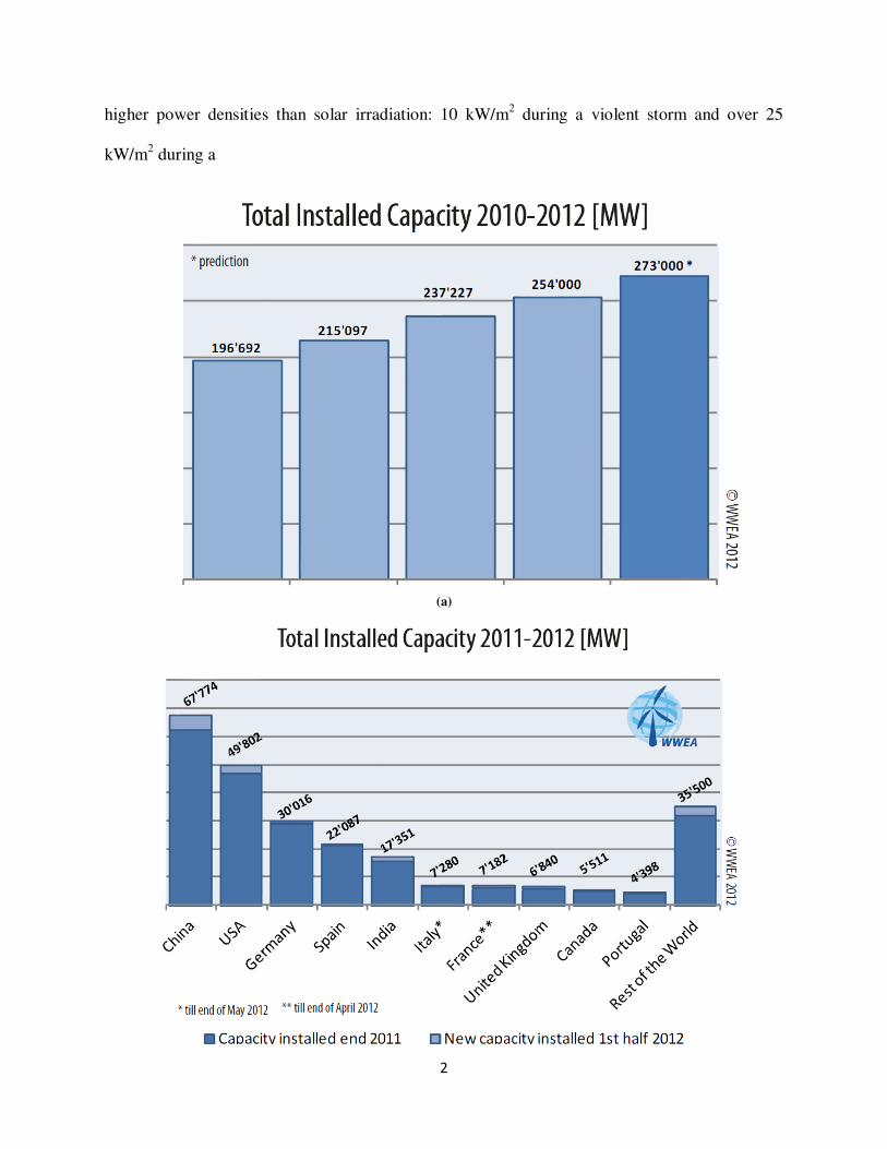
higher power densities than solar irradiation: 10 kW/m2 during a violent storm and over 25
kW/m2 during a
(a)

3
(b)
Fig. 1. 1 Total installed wind power capacity (a) in 2010-2012 (MW) around the world (b) in 2010-2012 (MW) in different countries [9].
hurricane, compared with the maximum terrestrial solar irradiance of about 1 kW/m2 [8].
However, a gentle breeze of 5 m/s has a power density only 0.075 kW/m2.
Wind energy is now achieving an exponential growth and has great potential in coming
decades. According to world wind energy association, there has been 16,5 GW of new
installations in the first half of 2012, after 18,4 GW in 2011. Worldwide wind capacity has
reached 254 GW by June 2012, and 273 GW expected by the end of 2012 [9].
The wind energy conversion systems (WECS) are complex, nonlinear and are subject to
parameters uncertainties and unknown disturbances [10]. For a fixed speed wind turbine
generators (WTG), rotor speed is constant at varying wind speed which reduces overall
efficiency considering power available in wind and extracted power. Using variable speed WTG
where rotor speed is controlled optimally, maximum power can be extracted from wind. Hence,
it is important to design a control technique which can track maximum power changing generator
speed optimally for wide speed range. Moreover, the controller has to be WT parameter
independent.
Control, monitoring, and protection of WTG usually require the information of wind
speed and generator rotor position. These can be measured by well-calibrated mechanical
sensors, such as anemometers and rotor position sensors. However, the use of these mechanical
sensors increases the cost and failure rate of the WTG systems. According to [11], sensor failures
contribute to more than 14% of failures in WTG systems and more than 40% of failures are
related to the failure of sensors and the consequent failures of the control or electrical systems.
Repairing the failed components requires additional cost and leads to a significant loss in electric

4
power production. It is important to design proper controller to track maximum power point of
wind turbine (WT) without relying on wind speed or rotor position sensors. In order to reduce
overall operating cost and expand rotor operating speed range, high efficiency power electronic
converters need to be implemented and sophisticated control algorithms should be developed to
extract optimal power at all atmospheric conditions.
1.2 Literature Survey on WECS
Wind energy harvesting has been a very long tradition. Some historians suggest that wind
mills were used over 3000 years ago. Until the early twentieth century wind power was used to
provide mechanical power to water pump, boats, ships and grinding mills. At the beginning of
the last century the first wind turbines appeared and technology was improved step by step from
the early 1970s. By the end of the 1990s, wind energy has come back as one of the most
important sustainable energy resources, partly because of the increasing price of the oil, security
concerns of nuclear power and its environmental issues [8].
1.2.1 Wind Energy Conversion
The sun heats up air masses in the atmosphere. The spherical shape of the Earth, the
Earth’s rotation and seasonal and regional fluctuations of the solar radiance cause spatial air
pressure differentials. These are the source of air movements. Wind resources are particularly
high in coastal areas because wind can move unhindered across the smooth surface of the sea.
Furthermore, temperature differences between water and land cause local compensating streams.
The sunlight heats the land more quickly than the water during the day. The results are pressure
differentials and compensating winds in the direction of the land.

5
Wind energy systems convert the kinetic energy of the wind into the electrical energy.
The kinetic energy produced by a moving object E is expressed by the following equation
[8]:
2
2
1skinetic mvE = (1.1)
Where, m and vs are mass and wind velocity of the object respectively.
The power (Pw) is this kinetic energy per unit time (joules /sec or watts).
2
2
1sw vmP
•
= (Assuming vs is constant) (1.2)
Here, •
m is the mass of air flowing per unit time, thus it can be defined as,
sAvm ρ=•
(1.3)
where, s - wind velocity; m - mass of air; A - swept area of the turbine blades; ρ- density of air
(1.225 kg/m3 @ sea level and 20° C)
So, mechanical power of due to wind flow can be written as,
3
2
1sw AvP ρ= (1.4)
When using wind rotors to extract wind power (i.e., wind turbine), it's not 100% efficient.
In 1919, a German physicist Albert Betz found limit of power conversion factor 16/27ths (i.e.,
59.3%) of the kinetic energy into mechanical power (Pm). This conversion factor is known as Cp
constant or Betz limit, and is a theoretical maximum coefficient of power for any wind turbine.

6
This constant is a measurement of how efficiently the wind turbine converts the energy in the
wind into electrical energy.
The power coefficient can be utilized in the form of a look-up tables or in form of a
function. The second approach is presented below, where the general function defining the
power coefficient as a function of the tip-speed ratio and the blade pitch angle is defined as [12],
)1(C
5x
431
2 1p
6
e ]CCCC[C),( µ
µβββλ
−
−−−=C 1.5)
31
035.0
08.0
11
ββλµ +−
+= , s
r
v
Rωλ =
, Pr
ωω =
(1.6)
where, C1= 0.5 , C2= 116 , C3= 0.4 , C4= 0 , C5= 5, C6= 21; β - pitch angle; ωr- shaft speed
[rad/s], ω- electrical angular velocity [rad/s], R - rotor radius [m]; vs - wind speed [m/s], l -tip
speed ratio, and P- pole pairs of the wind generator.
Wind speed model is given by the following equation:
(t)v(t)v(t)v(t)v(t)v ngrbs +++= (1.7)
where, vb-base wind component; vr- ramp wind component; vg- gust wind component; vn- base
noise wind component.
Therefore mechanical power available from wind turbine is given by,
),(³CAv½P psm βλρ= (1.8)
and mechanical torque is given by,
r
spm
vRCT
ωβλρ
π32
),(2
=
(1.9)
7
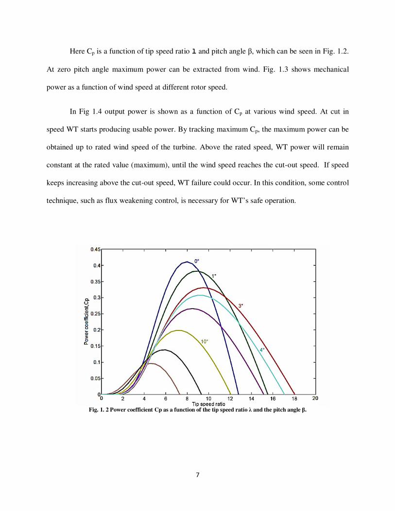
Here Cp is a function of tip speed ratio l and pitch angle β, which can be seen in Fig. 1.2.
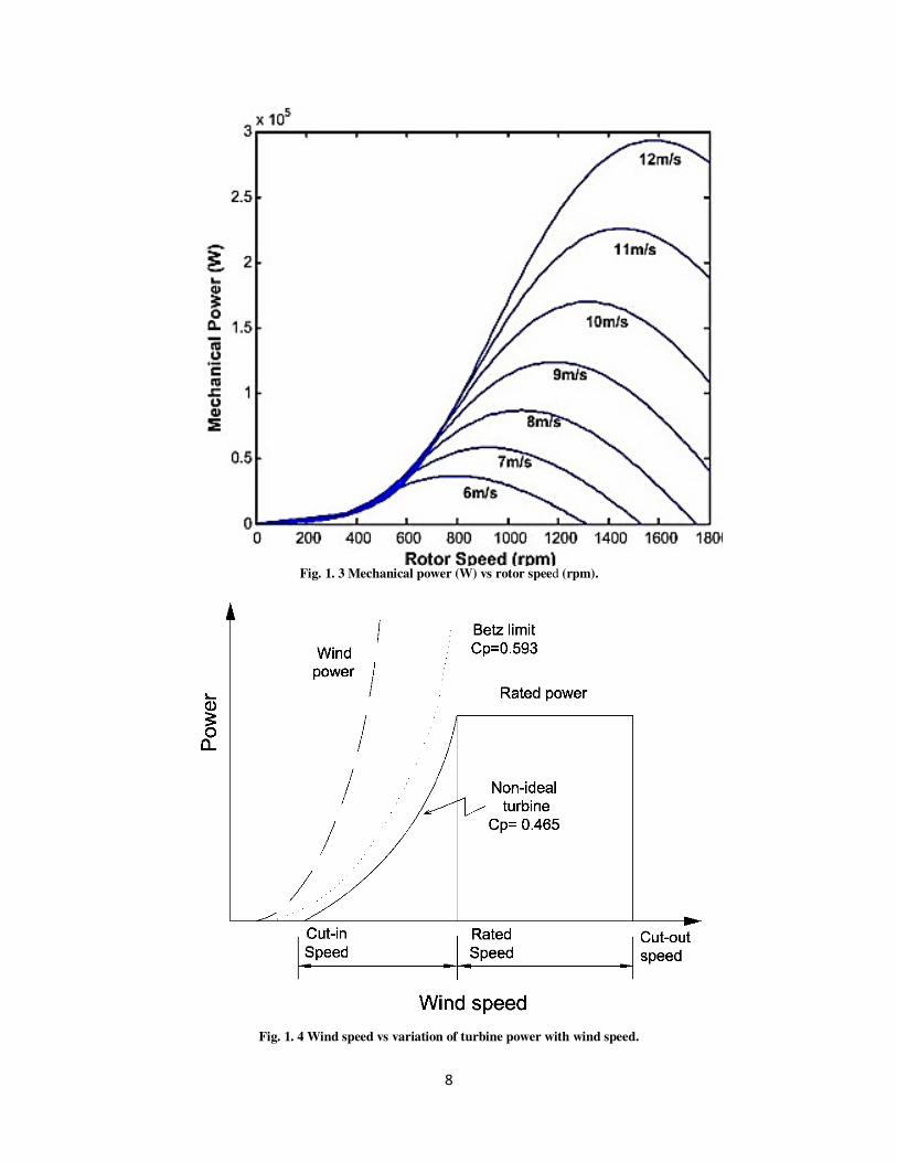
At zero pitch angle maximum power can be extracted from wind. Fig. 1.3 shows mechanical
power as a function of wind speed at different rotor speed.
In Fig 1.4 output power is shown as a function of Cp at various wind speed. At cut in
speed WT starts producing usable power. By tracking maximum Cp, the maximum power can be
obtained up to rated wind speed of the turbine. Above the rated speed, WT power will remain
constant at the rated value (maximum), until the wind speed reaches the cut-out speed. If speed
keeps increasing above the cut-out speed, WT failure could occur. In this condition, some control
technique, such as flux weakening control, is necessary for WT’s safe operation.
Fig. 1. 2 Power coefficient Cp as a function of the tip speed ratio λ and the pitch angle β.
8
Fig. 1. 3 Mechanical power (W) vs rotor speed (rpm).
Fig. 1. 4 Wind speed vs variation of turbine power with wind speed.
9
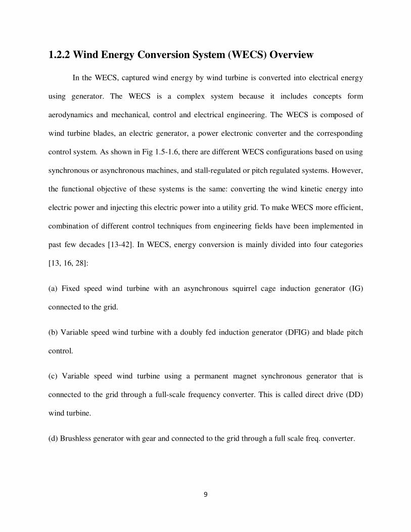
1.2.2 Wind Energy Conversion System (WECS) Overview
In the WECS, captured wind energy by wind turbine is converted into electrical energy
using generator. The WECS is a complex system because it includes concepts form
aerodynamics and mechanical, control and electrical engineering. The WECS is composed of
wind turbine blades, an electric generator, a power electronic converter and the corresponding
control system. As shown in Fig 1.5-1.6, there are different WECS configurations based on using
synchronous or asynchronous machines, and stall-regulated or pitch regulated systems. However,
the functional objective of these systems is the same: converting the wind kinetic energy into
electric power and injecting this electric power into a utility grid. To make WECS more efficient,
combination of different control techniques from engineering fields have been implemented in
past few decades [13-42]. In WECS, energy conversion is mainly divided into four categories
[13, 16, 28]:
(a) Fixed speed wind turbine with an asynchronous squirrel cage induction generator (IG)
connected to the grid.
(b) Variable speed wind turbine with a doubly fed induction generator (DFIG) and blade pitch
control.
(c) Variable speed wind turbine using a permanent magnet synchronous generator that is
connected to the grid through a full-scale frequency converter. This is called direct drive (DD)
wind turbine.
(d) Brushless generator with gear and connected to the grid through a full scale freq. converter.
10
(a)
(b)
(c)
11
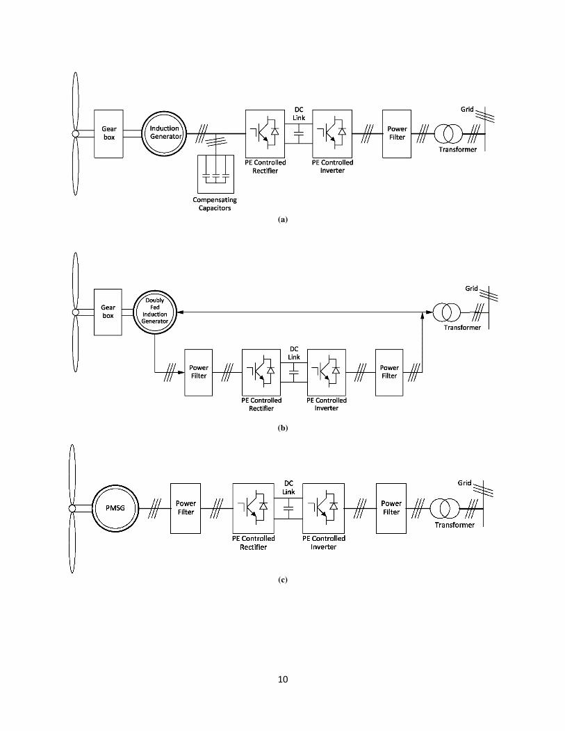
(d)
Fig. 1. 5 WECS categories (a) fixed speed wind turbine with an asynchronous squirrel cage IG (b) variable speed wind
turbine with a DFIG (c) variable speed wind turbine using PMSG (d) brushless generator with gear box.
Fig. 1. 6 Wind turbine generator types.
In fixed speed wind turbines, IGs are very commonly used. The wind turbine system in
Fig. 1.5(a) is using IG, which almost independent of torque variation operating at a fixed speed
with 2-3% slip condition. The power is limited aerodynamically either by stall, active stall or by
pitch control. All three systems are using a soft-starter in order to reduce the inrush current and
thereby limit flicker problems on the grid. They also need a reactive power compensator to
reduce the reactive power demand from the turbine generators to the grid. Those solutions are
12
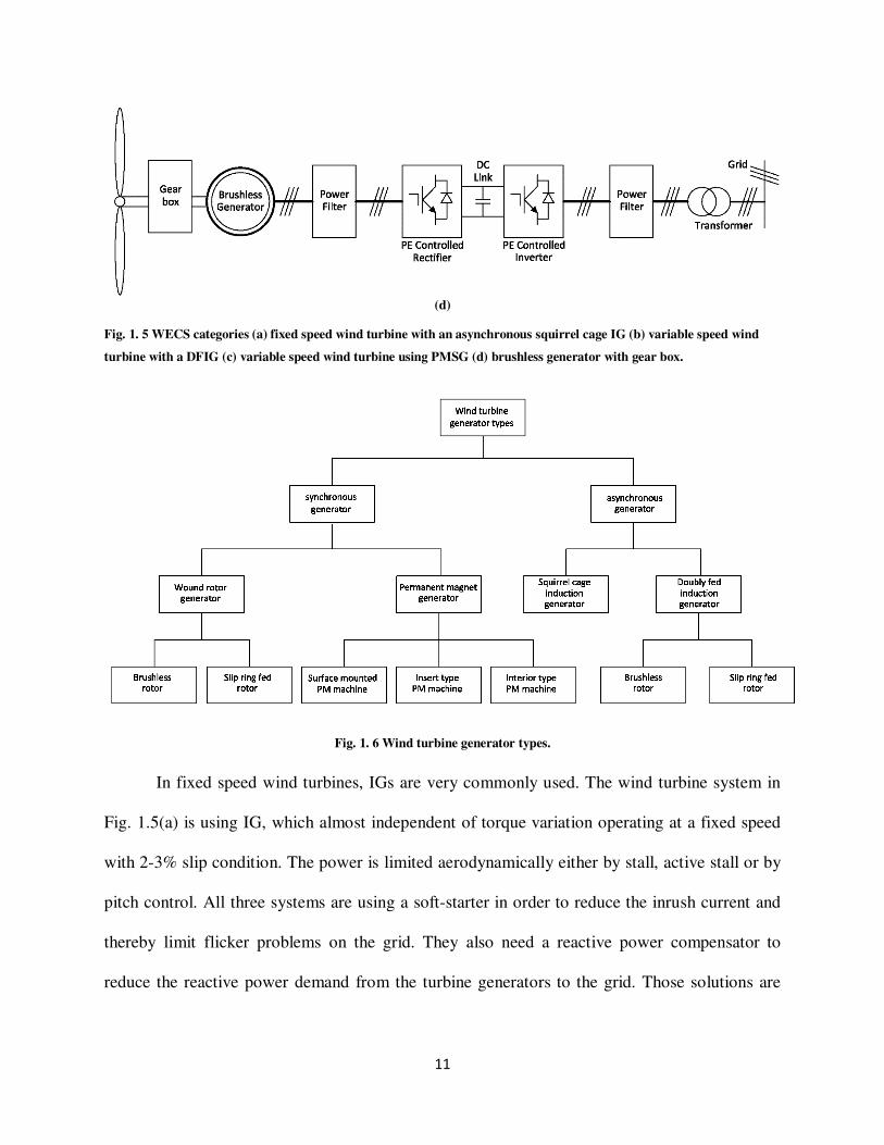
attractive due to low cost, but they are not able to control the active power very fast. Fig 1.7
shows the typical models of constant speed WT with gear box and direct drive WT.
(a) (b)
Fig. 1. 7 Sketch of (a) a constant speed WT with gear box (b) direct drive WT [13].
In contrast to direct grid connected IG, indirect grid connected wind turbines (including
wind turbines with DFIG - Fig 1.5(b)) are much more efficient because they could run at variable
speed condition. Additionally, these turbines can control reactive power to improve efficiency
for the electrical grid. The disadvantage for using the DFIG wind turbine is that the generator
uses slip rings. Since slip rings must be replaced periodically, and so the use of DFIGs need
frequent maintenance and require long term costs than other brushless generators [16]. The
PMSG connected to the grid by a full power back to back converter has become an attractive
alternative to the DFIG. This concept has several advantages such as the feasibility of direct
drive of the wind turbine with a PMSG of high number of poles, avoiding the use of a gearbox;
the high efficiency and high power density of PMSG; and the capability of the front end
converter to operate under network disturbances. Furthermore, the absence of a gearbox and the
lack of moving contacts on the PMSG increase the reliability and decreases the maintenance
13
requirements. With the advance of power electronics, PMSGs have drawn increased interest to
wind turbine manufacturers due to its advantages over other variable speed WTGs [29]. The
details about PMSG are discussed in the next chapter.
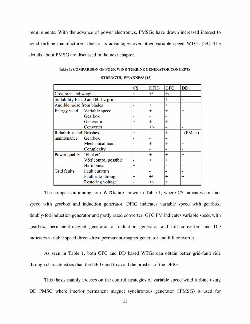
Table 1: COMPARISON OF FOUR WIND TURBINE GENERATOR CONCEPTS,
+ STRENGTH,-WEAKNESS [13].
The comparison among four WTGs are shown in Table-1, where CS indicates constant
speed with gearbox and induction generator, DFIG indicates variable speed with gearbox,
doubly-fed induction generator and partly rated converter, GFC PM indicates variable speed with
gearbox, permanent-magnet generator or induction generator and full converter, and DD
indicates variable speed direct-drive permanent-magnet generator and full converter.
As seen in Table 1, both GFC and DD based WTGs can obtain better grid-fault ride
through characteristics than the DFIG and to avoid the brushes of the DFIG.
This thesis mainly focuses on the control strategies of variable speed wind turbine using
DD PMSG where interior permanent magnet synchronous generator (IPMSG) is used for
14
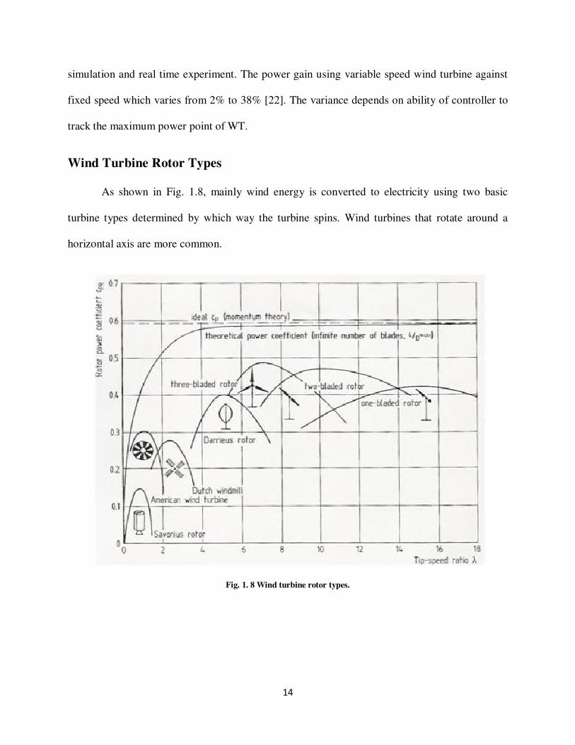
simulation and real time experiment. The power gain using variable speed wind turbine against
fixed speed which varies from 2% to 38% [22]. The variance depends on ability of controller to
track the maximum power point of WT.
Wind Turbine Rotor Types
As shown in Fig. 1.8, mainly wind energy is converted to electricity using two basic
turbine types determined by which way the turbine spins. Wind turbines that rotate around a
horizontal axis are more common.
Fig. 1. 8 Wind turbine rotor types.

15
(1) Horizontal Axis Wind Turbine (HAWT)
(a) 3 bladed Horizontal Axis Wind Turbine
Horizontal axis wind turbines are the more common style for commercial wind turbine.
The HAWT has blades that look like a propeller and spin on a horizontal axis. The most popular
turbine at the time is the 3 bladed HAWT as shown in Fig 1.9.
The HAWT has high efficiency, since the blades always move perpendicularly to the
wind, receiving power through the whole rotation; however, they require heavy construction to
support the heavy blades, gearbox, and generator housed in a nacelle on top of a large mast. The
HAWT have to be angled into the wind’s path, so that the wind’s direction is perpendicular to
the rotor plane. When the turbine is angled into the wind, the lift force from the aerodynamic
profiles will make the rotor turn. The advantages and disadvantages of HAWT as compared to
Vertical Axis Wind Turbine (VAWT) are summarized below.
Advantages of the HAWT:
• Higher efficiency
• Lower cost-to-power ratio
Disadvantages of the HAWT:
• More complex design required due to the need for yaw or tail drive
• Generator and gearbox should be mounted on a tower, which makes the maintenance
relatively more difficult
16
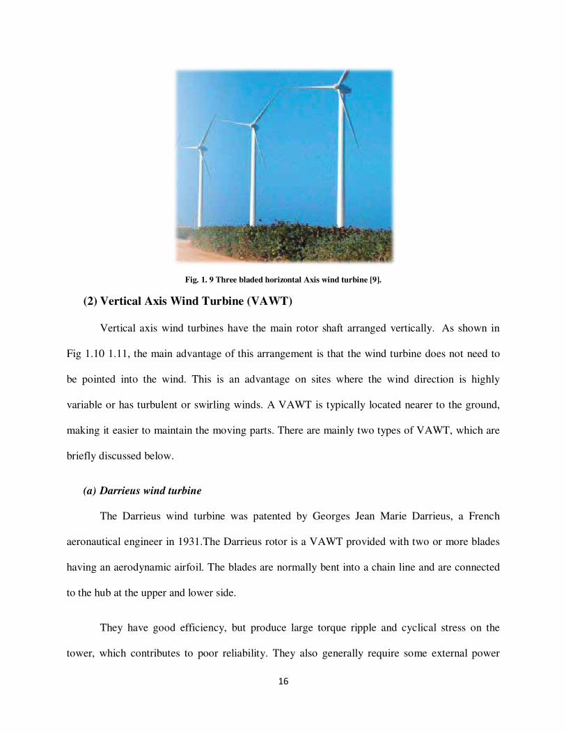
Fig. 1. 9 Three bladed horizontal Axis wind turbine [9].
(2) Vertical Axis Wind Turbine (VAWT)
Vertical axis wind turbines have the main rotor shaft arranged vertically. As shown in
Fig 1.10 1.11, the main advantage of this arrangement is that the wind turbine does not need to
be pointed into the wind. This is an advantage on sites where the wind direction is highly
variable or has turbulent or swirling winds. A VAWT is typically located nearer to the ground,
making it easier to maintain the moving parts. There are mainly two types of VAWT, which are
briefly discussed below.
(a) Darrieus wind turbine
The Darrieus wind turbine was patented by Georges Jean Marie Darrieus, a French
aeronautical engineer in 1931.The Darrieus rotor is a VAWT provided with two or more blades
having an aerodynamic airfoil. The blades are normally bent into a chain line and are connected
to the hub at the upper and lower side.
They have good efficiency, but produce large torque ripple and cyclical stress on the
tower, which contributes to poor reliability. They also generally require some external power

17
source, or an additional Savonius rotor to start turning, because the starting torque may be too
low to overcome the startup torque threshold of the generator.
Fig. 1. 10 Darrieus wind turbine [8].
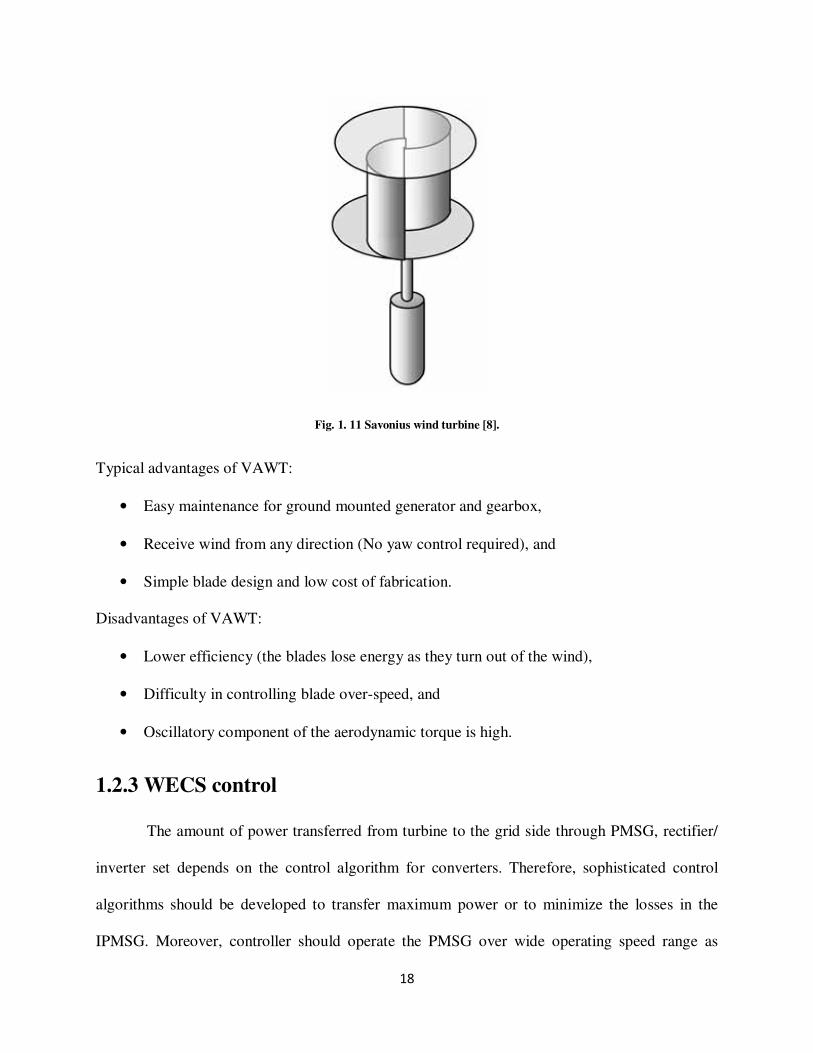
(b) Savonius wind turbine
Savonius wind turbine was invented by the Finnish engineer Sigurd J. Savonius in 1922. The
Savonius rotor consists of two hollow, half cylinders displaced from each other. Generally the
halves overlap by about one third of their diameter. The Savonius rotor can be constructed from
simple material using common tools. Savonius rotor concept never became popular, until
recently, probably because of its low efficiency. Its maximum power coefficient can reach up to
0.25 only [8].
18
Fig. 1. 11 Savonius wind turbine [8].
Typical advantages of VAWT:
• Easy maintenance for ground mounted generator and gearbox,
• Receive wind from any direction (No yaw control required), and
• Simple blade design and low cost of fabrication.
Disadvantages of VAWT:
• Lower efficiency (the blades lose energy as they turn out of the wind),
• Difficulty in controlling blade over-speed, and
• Oscillatory component of the aerodynamic torque is high.
1.2.3 WECS control
The amount of power transferred from turbine to the grid side through PMSG, rectifier/
inverter set depends on the control algorithm for converters. Therefore, sophisticated control
algorithms should be developed to transfer maximum power or to minimize the losses in the
IPMSG. Moreover, controller should operate the PMSG over wide operating speed range as
19
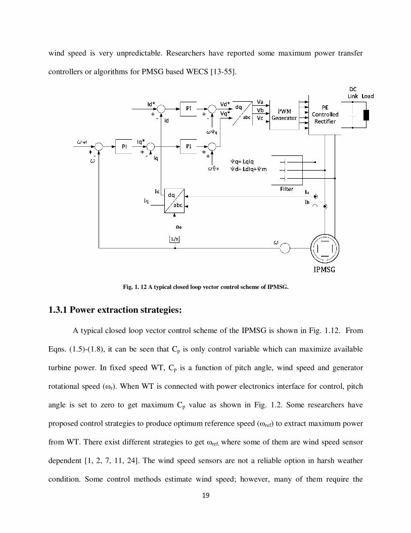
wind speed is very unpredictable. Researchers have reported some maximum power transfer
controllers or algorithms for PMSG based WECS [13-55].
Fig. 1. 12 A typical closed loop vector control scheme of IPMSG.
1.3.1 Power extraction strategies:
A typical closed loop vector control scheme of the IPMSG is shown in Fig. 1.12. From
Eqns. (1.5)-(1.8), it can be seen that Cp is only control variable which can maximize available
turbine power. In fixed speed WT, Cp is a function of pitch angle, wind speed and generator
rotational speed (ωr). When WT is connected with power electronics interface for control, pitch
angle is set to zero to get maximum Cp value as shown in Fig. 1.2. Some researchers have
proposed control strategies to produce optimum reference speed (ωref) to extract maximum power
from WT. There exist different strategies to get ωref, where some of them are wind speed sensor
dependent [1, 2, 7, 11, 24]. The wind speed sensors are not a reliable option in harsh weather
condition. Some control methods estimate wind speed; however, many of them require the

20
knowledge of air density and mechanical parameters of WECS [6, 12, 15, 21, 22, 29, 42-48].
With changing weather conditions, their controller output may vary. Moreover, rotating parts of
WECS may change their characteristics which could be an issue on performance over longer
period of time. Therefore, a lot of research efforts are focused on developing maximum power
point tracking (MPPT) controllers independent of wind speed senor and turbine parameters; for
example, hill-climb search type algorithm, optimum power search algorithm, etc. [19, 23, 30, 49-
55]. This algorithms can be very effective and can track optimum power online. Here, most of
the researchers who designed MPPT algorithms, did not show turbine power coefficient Cp graph
in their simulation results which explains maximum power tracking at different wind speed. In
[5], Cp graph is shown to explain MPPT, however, system operation is only shown for very
narrow wind speed operation. Some of them show the efficiency of generator for the maximum
power tracking operation of the system; however, their control doesn’t use any loss minimization
algorithm [55]. In [5, 11, 56, 57], intelligent control such as fuzzy logic and neural network
logic based power tracking have been presented. This controllers could provide good
performance in WECS as they don’t need exact parameters of the system. However, these
control techniques may increase complexity of the system, and add an extra calculation burden
on hardware side. Sometimes it could lead to run time errors and hence, prevent the system use
for real world applications.
1.3.2 Position and speed estimation:
Traditionally the rotor position is obtained from a shaft-mounted optical encoder or Hall
sensors. However, it is desirable to eliminate such sensors in PMSM drives to reduce system
costs and total hardware complexity, to increase the mechanical robustness and reliability, to
reduce the maintenance requirements, [59-83].

21
Authors reported different position and speed sensorless strategies in [59, 61, 80]. The
rotor position and angular speed of the IPMSM can be estimated by various methods. Position
estimation can be mainly divided into two categories. Non-adaptive methods and adaptive
methods. Non- adaptive methods use measured currents and voltages as well as fundamental
machine equations for estimation. On the other hand, adaptive estimation methods compare the
error between the measured output of the real system and the calculated estimated output of
machine model, and adapts the parameters of the model with the aim to minimize the error
between the real system and the model. The process of the adaptation is desired to be stable and
robust.
The simplest fundamental model methods are based on rotor flux position estimation, by
integrating the back-EMF [81]. It’s very simple but fails to estimate the rotor position at low and
zero rotor frequency. Low speed operation is critical in practical applications, since the estimated
rotor flux can be very sensitive to stator resistance variations, and inaccuracies. Among the
existing sensorless approaches, sliding mode has been recognized as a potential control approach
for electric machines. Previous studies show that sliding mode observers (SMO) have attractive
advantages of robustness to disturbances and low sensitivity to parameter variations [10, 66-68,
71, 72]. In [72] authors used sliding mode controller to estimate the induced back-EMF, rotor
position and speed. A sliding mode observer was built based on the electrical dynamic equations.
The back EMF information was obtained from the filtered switching signals relative to current
estimation error. To design the switching gain over a wide speed range based on this observer
model would be a challenging job.
The sensorless control methods presented in [73-75] based on Phase Locked Loop (PLL)
is simple, and easy to implement. In [64, 76-77], sensorless schemes that are based on the
22
application of flux observers (such as Kalman filter) have poor performance at low speed and
can be too complex and expensive to be used in practical systems. Signal injection schemes [63,
69, 79] can be more efficient, at low and zero speed, than any other sensorless estimation
scheme. In [69] authors investigated a high frequency signal injection method in such a way that
carrier-frequency voltages were applied to the stator windings of PMSM, producing high-
frequency currents whose magnitude varies with rotor position. The sensed currents were then
processed with a heterodyning technique that produced a signal approximately proportional to
the difference between the actual and the estimated rotor position. However, all these techniques
require high bandwidth and high precision measurement, and fast signal processing capability,
which may increase the complexity and cost of control system. The injected high-frequency
voltages may also cause more torque ripple, shaft vibration and audible noise.
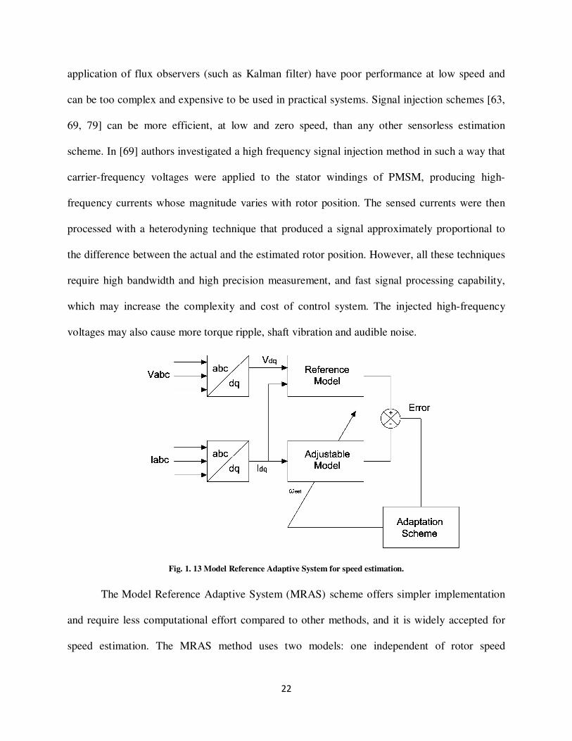
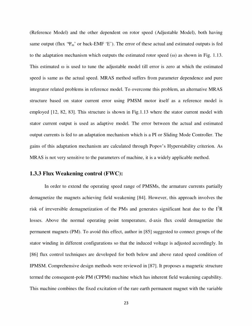
Fig. 1. 13 Model Reference Adaptive System for speed estimation.
The Model Reference Adaptive System (MRAS) scheme offers simpler implementation
and require less computational effort compared to other methods, and it is widely accepted for
speed estimation. The MRAS method uses two models: one independent of rotor speed
23
(Reference Model) and the other dependent on rotor speed (Adjustable Model), both having
same output (flux ‘Ψm’ or back-EMF ‘Ε’). The error of these actual and estimated outputs is fed
to the adaptation mechanism which outputs the estimated rotor speed (ω) as shown in Fig. 1.13.
This estimated ω is used to tune the adjustable model till error is zero at which the estimated
speed is same as the actual speed. MRAS method suffers from parameter dependence and pure
integrator related problems in reference model. To overcome this problem, an alternative MRAS
structure based on stator current error using PMSM motor itself as a reference model is
employed [12, 82, 83]. This structure is shown in Fig.1.13 where the stator current model with
stator current output is used as adaptive model. The error between the actual and estimated
output currents is fed to an adaptation mechanism which is a PI or Sliding Mode Controller. The
gains of this adaptation mechanism are calculated through Popov’s Hyperstability criterion. As
MRAS is not very sensitive to the parameters of machine, it is a widely applicable method.
1.3.3 Flux Weakening control (FWC):
In order to extend the operating speed range of PMSMs, the armature currents partially
demagnetize the magnets achieving field weakening [84]. However, this approach involves the
risk of irreversible demagnetization of the PMs and generates significant heat due to the I2R
losses. Above the normal operating point temperature, d-axis flux could demagnetize the
permanent magnets (PM). To avoid this effect, author in [85] suggested to connect groups of the
stator winding in different configurations so that the induced voltage is adjusted accordingly. In
[86] flux control techniques are developed for both below and above rated speed condition of
IPMSM. Comprehensive design methods were reviewed in [87]. It proposes a magnetic structure
termed the consequent-pole PM (CPPM) machine which has inherent field weakening capability.
This machine combines the fixed excitation of the rare earth permanent magnet with the variable

24
flux given by a field winding located on the stator. So, air-gap flux can be controlled over a wide
range with a minimum of conduction losses and without demagnetization risk for the PM pieces.
The efforts discussed above were made on the different types of PM machine design,
which has increased manufacturing cost due to the additional windings and/or complicated rotor
structure. On the other hand, many control strategies and algorithms have been developed for
flux-weakening operation of PMSM and published during the last decade [88-91]. In [88],
authors investigated a current-regulated flux-weakening method by introducing a negative
current component to create direct-axis flux in opposition to that of the magnetic flux, resulting
in a reduced air-gap flux. This armature reaction effect was used to extend the operating speed
range of PMSM and relieve the current regulator from saturation that can occur at high speeds.
In [89], author proposed FWC for surface-mounted permanent Magnet (SPM) machines which
did not require a knowledge of the machine or system parameters and was relatively simple
design. In [90], the flux-weakening is achieved by look-up table. The method is accurate and
easy to plan, but it needs a lot of test data, and the portability is poor. In [91] a review on the
state-of-the-art on flux-weakening control strategies for PMSMs are provided.
1.3 Objective of Thesis
The objectives of this thesis are to design, simulate and implement the control strategies
for variable speed WECS incorporating the MPPT algorithm for direct driven IPMSG. The
MPPT algorithm is designed based on a perturbation and observation algorithm. It is derived
based on active input power only and independent of wind speed. Thus, it makes the system
wind speed sensorless. In particular, the proposed objectives are as follows:

25
• To develop a new adaptive MPPT technique to transfer the maximum mechanical power
from WT to the dc-link.
• To incorporate wind speed sensorless approach with the proposed WECS.
• To incorporate the rotor position sensorless technique based on MRAS approach.
• To incorporate the field weakening technique to operate the machine over wide speed
range
• To simulate the overall IPMSG based WECS incorporating the proposed algorithms.
• To implement the proposed IPMSG based WECS in real-time using DSP board DS1104.
1.4 Thesis Organization
The present report consists of 6 chapters. Chapter 1 covers an overview of WECS. It
starts with an introduction to the subject. The advantages and disadvantages of the different types
of wind turbines and the two main kinds of wind energy systems are discussed. The literature
review, and objectives are also presented in this Chapter.
Chapter 2 provides general overview of the proposed WECS. The system components are
also described briefly. The modeling of Interior permanent magnet machine is presented. A brief
description of Space Vector Modulation (SVM) strategy to control the rectifier switches is also
provided.
In Chapter 3, a conventional control strategy for WECS has been discussed with
simulation results. The proposed novel adaptive MPPT algorithm with flux control is presented
in this Chapter. The performance of the proposed MPPT and FWC based WECS is investigated
in simulations.

26
Chapter 4 presents the developed rotor speed sensorless technique based MRAS
approach. The performance of the proposed MRAS based WECS is investigated in simulations.
Chapter 5 describes the real-time implementation of the 5 HP IPMSG drive system in
laboratory using dSPACE DS1104 DSP board. The experimental results of the MPPT based
rotor position sensorless control of IPMSG are shown in this Chapter. The detailed real-time
implementation procedures for both hardware and software are also discussed.
Finally, Chapter 6 presents summary/conclusions of this work and suggestions for future
work. The thesis concludes with references and appendices.
27
Chapter 2
Modeling of Wind Energy Conversion
System
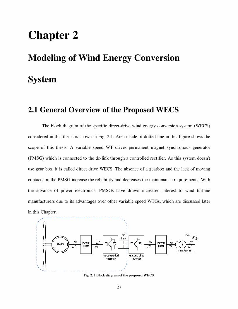
2.1 General Overview of the Proposed WECS
The block diagram of the specific direct-drive wind energy conversion system (WECS)
considered in this thesis is shown in Fig. 2.1. Area inside of dotted line in this figure shows the
scope of this thesis. A variable speed WT drives permanent magnet synchronous generator
(PMSG) which is connected to the dc-link through a controlled rectifier. As this system doesn't
use gear box, it is called direct drive WECS. The absence of a gearbox and the lack of moving
contacts on the PMSG increase the reliability and decreases the maintenance requirements. With
the advance of power electronics, PMSGs have drawn increased interest to wind turbine
manufacturers due to its advantages over other variable speed WTGs, which are discussed later
in this Chapter.
Fig. 2. 1 Block diagram of the proposed WECS.
28
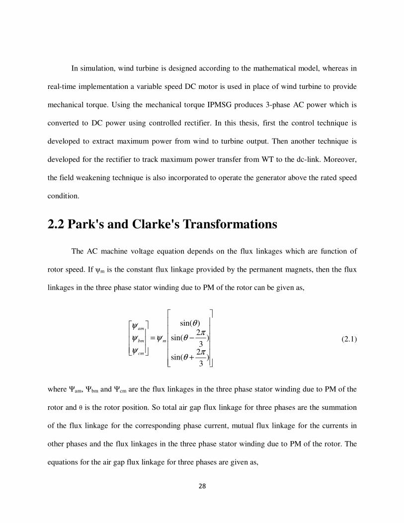
In simulation, wind turbine is designed according to the mathematical model, whereas in
real-time implementation a variable speed DC motor is used in place of wind turbine to provide
mechanical torque. Using the mechanical torque IPMSG produces 3-phase AC power which is
converted to DC power using controlled rectifier. In this thesis, first the control technique is
developed to extract maximum power from wind to turbine output. Then another technique is
developed for the rectifier to track maximum power transfer from WT to the dc-link. Moreover,
the field weakening technique is also incorporated to operate the generator above the rated speed
condition.
2.2 Park's and Clarke's Transformations
The AC machine voltage equation depends on the flux linkages which are function of
rotor speed. If ψm is the constant flux linkage provided by the permanent magnets, then the flux
linkages in the three phase stator winding due to PM of the rotor can be given as,
+
−=
)3
2sin(
)3
2sin(
)sin(
πθ
πθ
θ
ψ
ψ
ψ
ψ
m
cm
bm
am
(2.1)
where Ψam, Ψbm and Ψcm are the flux linkages in the three phase stator winding due to PM of the
rotor and θ is the rotor position. So total air gap flux linkage for three phases are the summation
of the flux linkage for the corresponding phase current, mutual flux linkage for the currents in
other phases and the flux linkages in the three phase stator winding due to PM of the rotor. The
equations for the air gap flux linkage for three phases are given as,

29
+
−+
=
)3
2sin(
)3
2sin(
)sin(
πθ
πθ
θ
ψ
ψ
ψ
ψ
m
c
b
a
cccbca
bcbbba
acabab
c
b
a
i
i
i
LMM
MLM
MML
(2.2)
where Ψa, Ψb and Ψc are the air gap flux linkage for the phase a, b, c, respectively; Laa,
Lbb, Lcc are the self-inductances and Mab, Mbc, Mca are the mutual inductances, respectively and θ
is rotor position. The phase voltage is the voltage drop in each phase plus the voltage drop due to
the rate of change of flux linkage. The voltage equations of the three phases of the IPMSM can
be defined as:
aa
a a
dv r i
dt
ψ= +
(2.3)
bb
b b
dv r i
dt
ψ= +
(2.4)
cc
c c
dv r i
dt
ψ= +
(2.5)
where va, vb, vc are the three phase voltages, ia, ib, ic are the three phase currents and ra, rb, rc are
the three phase stator resistances. These equations can be written in matrix form as,
a av 0 0
0 0
0 0
a a
b b b b
c cc c
ird
v r idt
rv i
ψ
ψ
ψ
= + (2.6)
va, vb and vc depends on the flux linkage components which are functions of rotor position θ and
hence functions of rotor speed ω. Therefore, the coefficients of the voltage equations are time

30
varying except when the machine is motionless. In order to keep away from the difficulty of
calculations, all the equations have to be changed to the synchronously rotating rotor reference
frame where the machine equations are no longer dependent on the rotor position. These
transformations can be achieved in two steps using Clarke’s and Park’s transformation equations
[92]. In the first step, va, vb and vc will be transformed from the three phase stationary a-b-c
frame into two phase stationary α-β frame and in the second step, from the stationary α-β frame
to the synchronously rotating d-q frame. The transformed phase variables in the stationary d-q-0
axis can be written in matrix form as:
+
+
−
−=
0
13
2sin
3
2cos
13
2sin
3
2cos
1)sin()(cos
x
x
x
x
x
x
c
b
a
α
β
πθ
πθ
πθ
πθ
θθ
(2.7)
The corresponding inverse relation can be written as:
+−
+−
=
c
b
a
x
x
x
s
x
x
x
2
1
2
1
2
1
)3
2sin()
3
2sin()in(
)3
2cos()
3
2cos()(cos
3
2
0
πθ
πθθ
πθ
πθθ
α
β
(2.8)
where, xa, xb and xc are the a, b and c phase quantities, respectively, xα, xβ and x0 are the α -axis,
β -axis and zero sequence components, respectively. The matrix element x may represent either
voltage or current.
The rotor location or rotor position angle θ is defined as:

31
)0()()(0
θδδωθ += ∫t
d (2.9)
where, δ is a dummy variable.
For balanced three phase, zero sequence component (x0) does not exist, and it is
convenient to set initial rotor position θ(0) = 0 so that the q-axis coincides with a-phase. Under
these conditions Eqns. (2.7) and (2.8) can be written, respectively, as:
−
−−=
α
β
x
x
x
x
x
c
b
a
2
3
2
1
2
3
2
1
01
(2.10)
and
−−
−−
=
c
b
a
x
x
x
x
x
3
1
3
10
3
1
3
1
3
2
α
β (2.11)
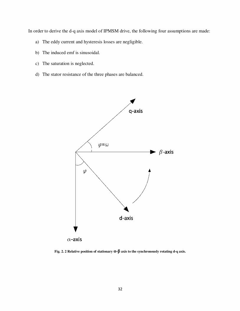
The relative position of the stationary α-β frame and the synchronously rotating d-q frame is
shown in Fig. 2.2. With the help of Fig. 2.2 the stationary α-β frame can be converted to the
synchronously rotating d-q frame as:
−=
α
β
θθ
θθ
x
x
x
x
d
q
cossin
sincos (2.12)
The inverse relation can be written as:
−=
d
q
x
x
x
x
θθ
θθ
α
β
cossin
sincos (2.13)
32
In order to derive the d-q axis model of IPMSM drive, the following four assumptions are made:
a) The eddy current and hysteresis losses are negligible.
b) The induced emf is sinusoidal.
c) The saturation is neglected.
d) The stator resistance of the three phases are balanced.
Fig. 2. 2 Relative position of stationary α-β axis to the synchronously rotating d-q axis.

33
2.3 Introduction to Permanent Magnet Synchronous
Machines
Recently, the PMSG has received much attention in wind energy application because of
its several advantages such as high efficiency, high power density, less maintenance robustness
over the conventional ac machines utilized for WECS [17]. Furthermore, the PMSGs do not need
additional power for rotor excitation as the flux is supplied by the permanent magnets.
Current improvement of PMSG is directly associated to the recent achievement in high
energy permanent magnet materials. Ferrite and rare earth/cobalt alloys such as neodymium-
boron-iron (Nd-B-Fe), samarium-cobalt (Sm-Co) are widely used as magnetic materials. Rare
earth/cobalt alloys have a high residual induction and coercive force than the ferrite materials.
But the cost is also relatively high. So rare earth magnets are usually used for high performance
variable speed drive as high torque to inertia ratio is desirable
The classification for PMSM can be done based on some different principle such as
design of the machine, driving power circuit configuration, position of magnet in the rotor,
current regulation and the principal machine control method. The performance of a PMSM drive
varies with the magnet material, placement of the magnet in the rotor, configuration of the rotor,
the number of poles, EMF waveform and the presence of dampers on the rotor [93, 94].
Depending on magnet configuration, it can be categorized into three divisions.

34
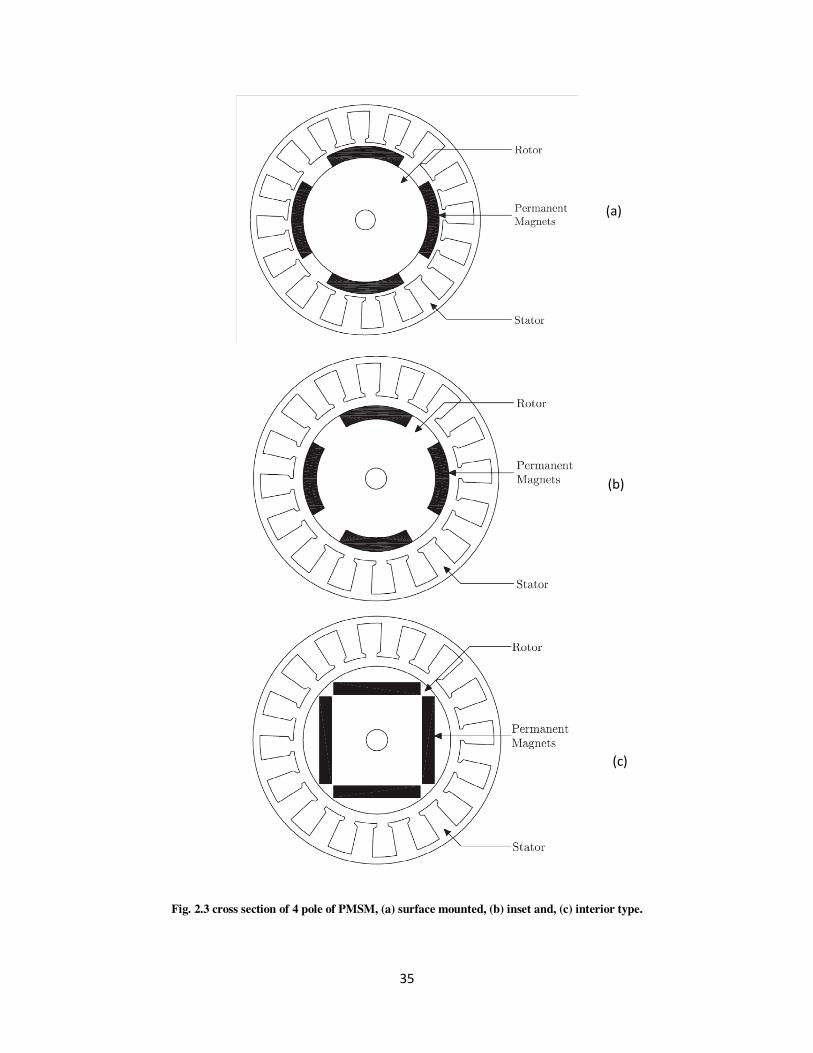
(a) Surface mounted PM machine:
In this type of PM machine, the PMs are typically glued or banded with a non-conducting
material to the surface of the rotor core as shown in Fig.2.4 (a). This type of machine is not
suitable for high speed.
(b) Inset type PM machine:
In this type of PM machine, the PMs are typically glued directly or banded with a non-
conducting material inside the rotor core as shown in Fig.2.4 (b). This type of machine is not
suitable for high speed.
(c) Interior type PM machine:
In this type of PM machine, the PMs are imbedded in the interior of the rotor core as
shown in Fig.2.4 (c). Interior magnet designs offer q-axis inductance larger than the d-axis
inductance. The saliency makes possible a degree of flux weakening, enabling operation above
nominal speed at constant voltage and should also help to reduce the harmonic losses in the
machine. This kind of PM machine has the same advantages of inset machine as well as the
advantages of mechanical robustness and a smaller magnetic air gap. Therefore, the interior type
PM synchronous machine (IPMSM) is more suitable for high speed operations.
35
Fig. 2.3 cross section of 4 pole of PMSM, (a) surface mounted, (b) inset and, (c) interior type.
(a)
(b)
(c)

36
An interior permanent magnet (IPM) synchronous generator can produce more energy
compared to surface PMSG which is used in this thesis to make the system more efficient.
IPMSG can offer high efficiency and high-controllability generation by utilizing the reluctance
torque as well as magnetic torque as both d- and q- axis components of stator current contribute
to the torque development process. Therefore, in this thesis the IPMSG is considered for WECS.
2.4 Mathematical Model Development
These voltage equations depend on the flux linkage components which are function of
rotor position θ and the coefficients of the voltage equations are time varying except when the
machine is motionless. In order to keep away from the difficulty of calculations, all the equations
have to be changed to the synchronously revolving rotor reference frame where the machine
equations are no longer dependent on the rotor position. These transformations can be
accomplished in two steps using Park’s transformation equations.
Fig. 2. 4 Equivalent circuits of IPMSM (a) d-axis equivalent circuit. (b) q-axis equivalent circuit.

37
d
q
sqqdt
dRiv ωψ
ψ++= (2.14)
q
d
sdddt
dRiv ωψ
ψ−+= (2.15)
where vd, vq are d-q axis voltages and id, iq
are d-q axis currents, ψd, ψq are d-q axis flux linkages
and R is the stator resistance per phase and ω is the electrical angular velocity. ψd and ψq can be
written as,
ψq = Lqiq (2.16)
ψd= Ldid + ψm (2.17)
where, Ld and Lq are d- q-axis self-inductances.
so eq. 2.14 and 2.15 becomes
d
dsdd iLdt
diLRiv ω−+= (2.18)
mdd
q
qsqq iLdt
diLRiv ωψω +++= (2.19)
When using lumped mass model as given in equation below for WT generator shaft system, the
motion equation of IPMSG can be expressed as:
rmemr BTT
dt
dJ ω
ω−−= (2.20)
where, J - total moment of inertia of the wind turbine (Kg.m2), Bm- Viscous damping coefficient
(Kg.m2/s), Tm- input mechanical torque (Nm) given by,

38
Tm=Pm/ωr (2.21)
ωr= 2ω/Pn (2.22)
where, ωr is rotor speed (rad/sec), Pn - Number of poles of IPMSG
Electrical torque (Te) equation is given by:
)(22
3oqodqdoqm
n
e iiLLiP
T −+= ψ (2.23)
Considering core loss resistance (Rc), the IPMSM’s dynamic model can be represented
mathematically in d-q synchronous rotating frame as [38].
−
++=
oqqod
d
c
sodsd
ILdt
diL
R
RiRv ω1 (2.24)
+−
++= )(1
modd
oq
q
c
s
oqsqIL
dt
diL
R
RiRv ψω (2.25)
Where iod and ioq are d-axis demagnetizing and q-axis torque generating currents
respectively, icd and icq are d-q axis core loss currents respectively.
Copper and core losses are the two losses in IPMSM. Eddy current losses are caused by
the flow of induced currents inside the stator core and hysteresis losses are caused by the
continuous variation of flux linkages and frequency of the flux variation in the core. On the other
hand copper loss, Pis due to current flow through the stator windings. Based on Fig. 2.4 the
copper lossP and iron loss P in steady state are expressed as follows:
22
22 )(
2
3)(
2
3
+++
−=+=
c
oddmoqs
c
oqd
odsqdscuR
iLiR
R
iLiRiiRP
ψωωσ (2.26)

39
22
2
22 )(
2
3
2
3)(
2
3
++
=+=
c
oddm
c
c
oqd
ccqcdcFeR
iLR
R
iLRiiRP
ψωωσ (2.27)
where, σ is Lq/Ld. The efficiency of WECS is defined as,
%100m
o
P
P=η (2.28)
dcdco IVP = (2.29)
where, Pm is the output power of WT, Po is DC-link power, and Vdc and Idc are DC-link
voltage and current respectively.
2.5 Vector Control of IPMSM
Vector control is the most popular control technique of AC machine. In d-q reference
frames, the expression for the electromagnetic torque of the smooth-air-gap machine is similar to
the expression for the torque of the separately excited DC machine. In the case of PM machine,
the control is usually performed in the reference frame (d-q) attached to the rotor flux space
vector. In case of dc motor, the developed torque is given by,
afe IKIT = (2.30)
where Ia is the armature current, If is the field current and K is a constant. Both Ia and If are
orthogonal and decoupled vectors. So the control becomes easier for separately excited dc motor.
In case of PM machine the first term of torque Eqn. (2.30) represents the magnet torque
produced by the permanent magnet flux and q axis current and the second term represents the
reluctance torque produced by the interaction of q and d axis inductances and the d-q axis

40
currents. Most of the researchers consider the command d-axis current, id=0. So that the torque
equation becomes linear with iq and control task becomes easier.
With id = 0, Te becomes,
3
2e q t q
PT i K iψ= =
(2.31)
However with the assumption of id=0, as per Eqn. (2.31), the flux cannot be controlled in an
IPMSM. Without a proper flux control, machine cannot be operated above the rated speed while
maintaining voltage and current within the rated capacity of the machine/converter. In the
proposed work, the flux will be properly controlled so that the machine can be controlled
efficiently below and above the rated speed. Thus, the IPMSM can be controlled like a separately
excited DC motor where iq controls the torque and id controls the flux.
Using phasor notation and taking the d axis as the reference phasor, the steady state phase
voltage Va can be derived from steady state d-q axis voltage using equation (2.14) and (2.15) as,
qda jVVV +=
mrddrqqras jiLjiLIR ψωωω ++−= (2.32)
where, the phase current is:
qda jiiI +−= (2.33)
In the case of IPM machine, the d axis current is negative and it demagnetizes the main
flux provided by the permanent magnets. Thus in order to take the absolute value of id we can
rewrite the equation as,
41
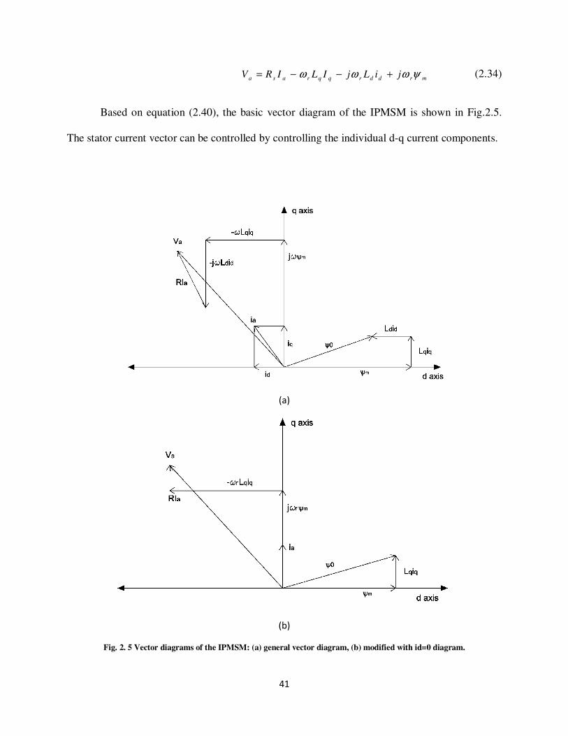
mrddrqqrasa jiLjILIRV ψωωω +−−= (2.34)
Based on equation (2.40), the basic vector diagram of the IPMSM is shown in Fig.2.5.
The stator current vector can be controlled by controlling the individual d-q current components.
(a)
(b)
Fig. 2. 5 Vector diagrams of the IPMSM: (a) general vector diagram, (b) modified with id=0 diagram.
42
2.6 Space-Vector Pulse Width Modulation of the
Voltage Source Converter
A 3-phase controlled rectifier circuit to convert the ac output voltage of IPMSG to a fixed
dc voltage is shown in Fig. 2.6. The rectifier switches (S1-S6) can be controlled using well-
known pulse width modulation technique (PWM).
Fig. 2. 6 Simplified representation of three-phase PWM rectifier.
Pulse width modulation has been studied extensively during the past decades. Many
different PWM methods have been developed to achieve the following aims: wide linear
modulation range; low switching loss; low total harmonic distortion (THD) in the spectrum of
switching waveform; and easy implementation and low computation time [95]. There are many
possible PWM techniques have proposed in past decades. The classifications of PWM
techniques can be given as follows:
o Sinusoidal PWM (SPWM)
o Selected harmonic elimination (SHE) PWM
IPMSG

43
o Minimum ripple current PWM
o Space vector PWM (SVM)
o Random PWM
o Hysteresis band current control PWM
o Sinusoidal PWM with instantaneous current control
o Delta modulation
o Sigma-delta modulation
The space-vector PWM method is an advanced, low computation PWM method and is
possibly the best among all PWM techniques for variable frequency drive applications [96]. It
uses the space-vector concept to compute the duty cycle of the switches.
Fig. 2.7 shows the topology of the typical three-phase PWM rectifier circuit. There are
six switching regions, which are determined by the angle of phase input voltages. The upper and
lower switches in each phase are always operated complementary. Switches of two phases are
driven by PWM mode while ones of another phase are always turned on or off during each
region. Table 2.1 summarizes the switching schemes and the available voltage vectors in each
region. The voltage space vector diagram and the switching logics of upper switches (S1, S3, and
S5) for each voltage vector can be seen in Table 2.1.
Fig. 2. 7 Voltage space vector diagram.

44
Table 2.1: SWITCHING SCHEME AND AVAILABLE VOLTAGE VECTORS IN EACH
REGION [97]
Region S1 S2 S3 S4 S5 S6 Available Voltage Vectors
1 PWM PWM OFF ON PWM PWM V5,V6,V1,V8
2 ON OFF PWM PWM PWM PWM V6,V1,V2,V7
3 PWM PWM PWM PWM OFF ON V1,V2,V3,V8
4 PWM PWM ON OFF PWM PWM V2,V3,V4,V7
5 OFF ON PWM PWM PWM PWM V3,V4,V5,V8
6 PWM PWM PWM PWM ON OFF V4,V5.V6,V7
2.7 Concluding Remarks
This Chapter has provided a general overview of proposed WECS system. The detail
mathematical model of IPMSM has been derived. The vector control technique for IPMSM has
also been introduced in this Chapter. An overview of space-vector pulse width modulation
technique to control the rectifier switches has also been provided.

45
Chapter 3
Power Extraction Strategies and Control
Techniques
Electricity is an integral part in the development of modern society and life without
electricity is unimaginable in developed countries. In many countries, with increased population
and necessities, demand of electricity has been increasing rapidly and at the same time
conventional power sources are limited. Renewable energy sources are becoming a good
solution to these issues. Among the renewable energy sources, wind energy is one of the fastest
growing, cost effective and environmental friendly way of electricity generation. However, it is
important to extract the maximum power available from variable wind conditions.
In wind energy conversion system output power is maximum at particular rotor speed for
a given wind speed. Fig. 3.1 shows the power coefficient CP vs tip speed ratio (λ). It is seen that
the maximum Cp can be obtained at the specific TSR value. To further explain this concept, Fig.
3.2 shows the typical WT and generator power curve at different rotor speed for different wind
velocities. Maximum turbine power (Pm max) and generator power (Pe max) are the maximum
power points at different rotor speed with changing wind. It is desired that the maximum power
controller follows that generator power curve at variable wind speed. As shown in Eqns. (1.6 and

46
1.7), mechanical output power is a function of TSR, so maximum power is extracted at optimum
TSR. Rotor speed is a controllable variable in TSR equation. The rotor speed can be controlled
mechanically or electrically. It can be achieved by changing pitch angle of the turbine rotor
(mechanically) or changing load on the generator (electrically). With unpredictable wind speed
change, mechanical control is not feasible. Mechanical elements suffers from considerable faults
and increasing maintenance expenses [5]. To make the control efficient and robust, generator
terminal voltage needs to be controlled using some power converter such a way that rotor speed
corresponds to optimum TSR with changing wind speed. The load at the generator can be
changed by controlled rectifier converter as discussed in Chapter 2.
Several types of control schemes such as duty cycle control, look up table for optimum
rotor speed and optimum TSR have been proposed to improve the performance of wind power
extraction [1, 2, 7, 6, 12, 15, 19-26]. However, these schemes depend on wind turbine
characteristics (torque, power and power coefficient curves) or wind speed either before or
during execution. Wind turbine components tend to change their characteristics over the time;
moreover, some of these strategies are customized for a particular turbine. In addition, they don’t
take atmospheric change in air density into consideration which plays significant part in the
aerodynamics of the turbine.
Control strategy independent of WT characteristics, such as perturbation and observation
(PO) method is very flexible and accurate [23]. Optimum power search algorithm proposed in
this work tracks peak power points in P-ω (power-speed) curve corresponds to dP/dω = 0. In [5]
neural network based MPPT algorithm and in [11] back propagation neural network based
MPPT algorithm are proposed.
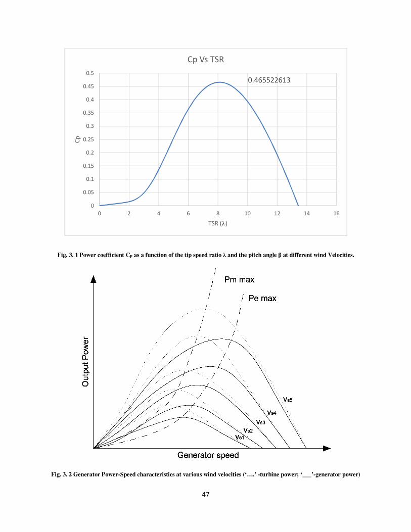
47
Fig. 3. 1 Power coefficient CP as a function of the tip speed ratio λ and the pitch angle β at different wind Velocities.
Fig. 3. 2 Generator Power-Speed characteristics at various wind velocities (‘….’ -turbine power; ‘___’-generator power)
0.465522613
0
0.05
0.1
0.15
0.2
0.25
0.3
0.35
0.4
0.45
0.5
0 2 4 6 8 10 12 14 16
Cp
TSR (λ)
Cp Vs TSR
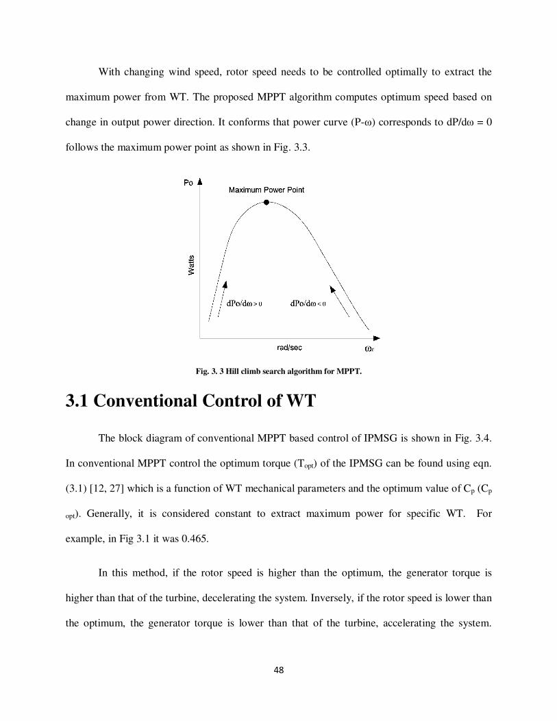
48
With changing wind speed, rotor speed needs to be controlled optimally to extract the
maximum power from WT. The proposed MPPT algorithm computes optimum speed based on
change in output power direction. It conforms that power curve (P-ω) corresponds to dP/dω = 0
follows the maximum power point as shown in Fig. 3.3.
Fig. 3. 3 Hill climb search algorithm for MPPT.
3.1 Conventional Control of WT
The block diagram of conventional MPPT based control of IPMSG is shown in Fig. 3.4.
In conventional MPPT control the optimum torque (Topt) of the IPMSG can be found using eqn.
(3.1) [12, 27] which is a function of WT mechanical parameters and the optimum value of Cp (Cp
opt). Generally, it is considered constant to extract maximum power for specific WT. For
example, in Fig 3.1 it was 0.465.
In this method, if the rotor speed is higher than the optimum, the generator torque is
higher than that of the turbine, decelerating the system. Inversely, if the rotor speed is lower than
the optimum, the generator torque is lower than that of the turbine, accelerating the system.
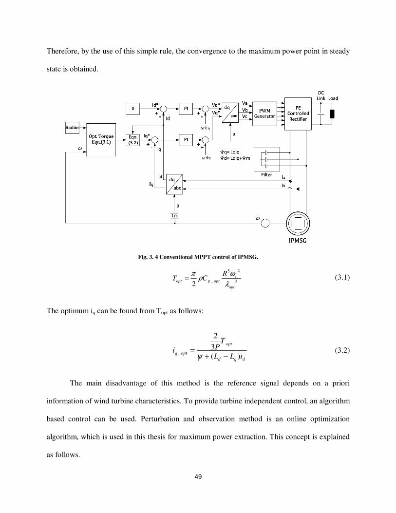
49
Therefore, by the use of this simple rule, the convergence to the maximum power point in steady
state is obtained.
Fig. 3. 4 Conventional MPPT control of IPMSG.
3
25
_2
opt
roptpopt
RCT
λ
ωρ
π= (3.1)
The optimum iq can be found from Topt as follows:
dqd
opt
optqiLL
TPi
)(
3
2
_−+
=ψ
(3.2)
The main disadvantage of this method is the reference signal depends on a priori
information of wind turbine characteristics. To provide turbine independent control, an algorithm
based control can be used. Perturbation and observation method is an online optimization
algorithm, which is used in this thesis for maximum power extraction. This concept is explained
as follows.

50
3.2 Proposed MPPT Algorithm
The proposed adaptive MPPT controller uses perturbation and observation (PO) based
algorithm. Estimated power output Pe is calculated based on sensed currents and voltages. This
power is sampled to check the changes in direction and difference between previous and current
value (∆Pe). ∆Pe is checked if it's within the adequate range, then the optimum speed reference
value remains same.
The flow chart for the proposed MPPT algorithm based PO method is shown in Fig 3.5.
X is the control variable, which is considered as rotor speed for this thesis. According to the
direction of ∆Pe and ∆X, sign is assigned for optimum step change in speed which is shown in
Table 4.1.
Table 4.1: Sign deciding table for control variable step:
∆Pe ∆X Sign ∆Xstep
+ + +
+ - -
- + -
- - +
The sign is multiplied with ∆Pe and variable 'K' to find optimum ∆X. Here, K is a
function of X which is designed in such a way that it gives larger value of ∆X at low and high
value of X. The following function is developed to adapt the coefficient K with the value of X
based on trial and error in simulation so that the MPPT algorithm converges faster.
2.01e*2- K ))300)-*(x(-0.00022
+= (3.3)
Optimum speed reference is found by adding ∆X to previous value of X. As shown in
Fig. 3.6 optimum speed is tracked to extract maximum power at different wind speeds. The curve
connecting to A-B-C shows the path of maximum power points.
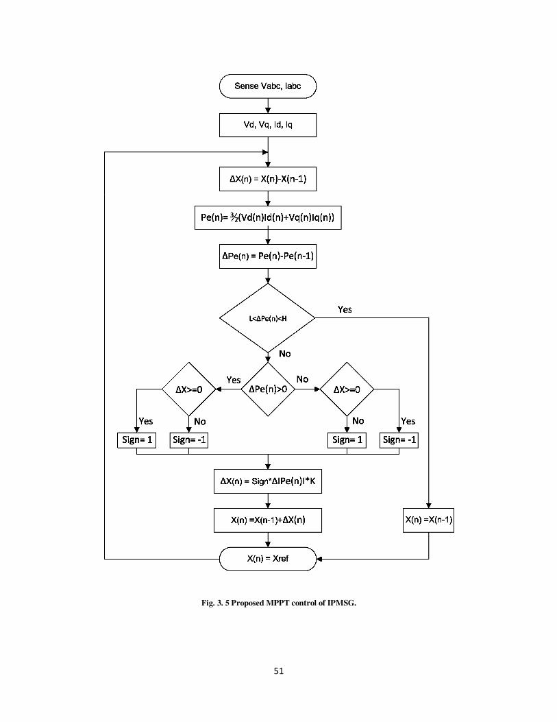
51
Fig. 3. 5 Proposed MPPT control of IPMSG.

52
Fig. 3. 6 Change of operating point for MPPT.
3.3 Overall Control of the Proposed WECS System
The block diagram of the control structure for the proposed WECS with MPPT algorithm
and flux weakening control (FWC) algorithm is shown in Fig. 3.7. The phase currents and
voltages are converted into d-q axis quantities to control torque and the flux of IPMSG
respectively. The reference speed ω* is generated based on newly developed MPPT algorithm,
which is compared with actual speed of IPMSG. The speed error is processed through speed
controller which gives the q-axis command current iq* as output. To control generator flux, d-
axis command current id* is controlled by maximum torque per ampere if the speed is below
rated speed, and FWC if it is above rated. Obtained d-q axis command voltages from id* and iq*
generates PWM signals for generator side controlled rectifier. On dc-link resistive load is
connected across low pass filter. Capacitive bank is connected between IPMSG and controlled
rectifier to filter out voltage spikes generated by rectifier.
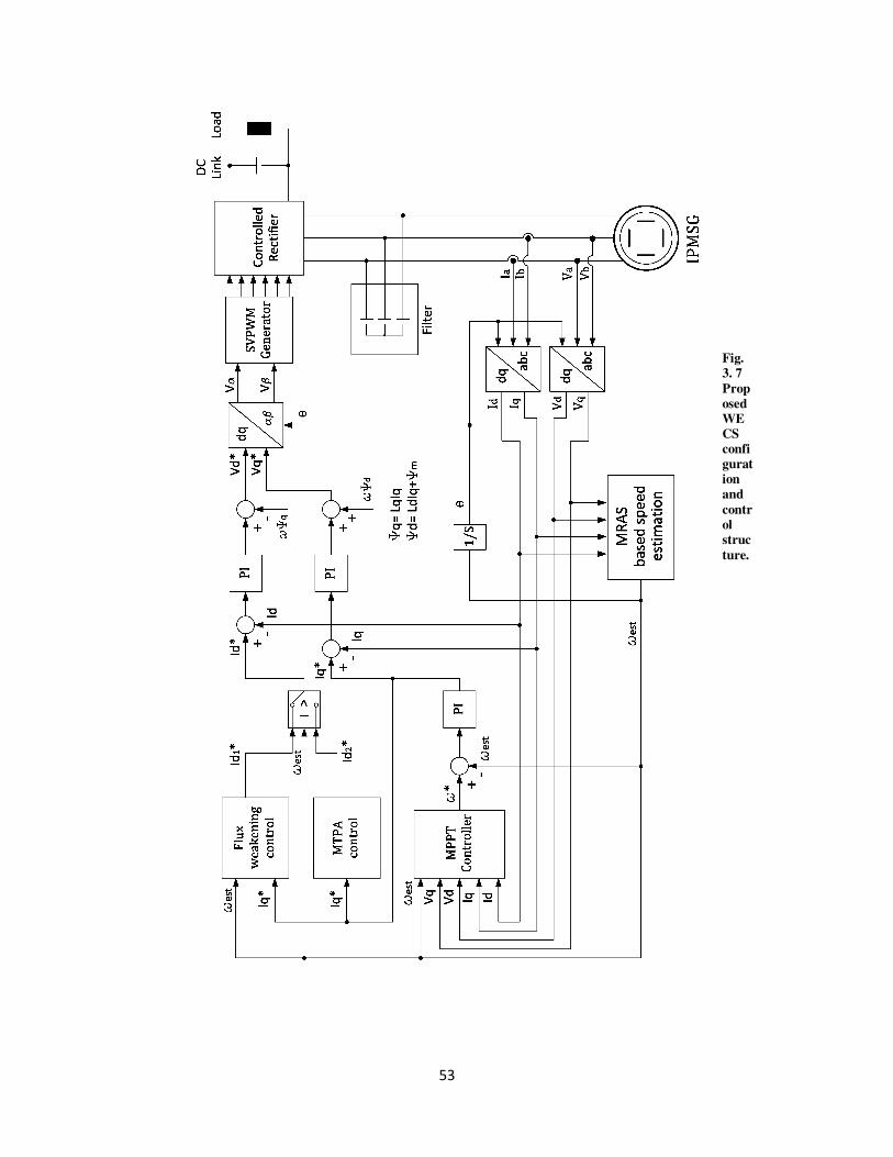
53
Fig.
3. 7
Prop
osed
WE
CS
confi
gurat
ion
and
contr
ol
struc
ture.

54
3.4 Flux Controller Design
Precise control of the high performance IPMSG over a wide speed range is an
engineering challenge. Traditionally in the design of the controller, id = 0 is taken to make the
control task easier with this assumption the flux supplied by the permanent magnet remains
constant. Moreover, the assumption of id = 0 leads to a non-optimum efficiency and sometimes
instability of the IPMSM even below the base rotor speed. The speed is inversely proportional to
the flux due to permanent magnet and proportional to the back EMF. In order to operate the
machine above the base speed within the rated voltage capacity of the generator and the rectifier,
the field flux must be weakened. In the case of the IPMSG, direct control of the field flux is not
possible. However, the field flux can be weakened by the demagnetizing effect of the d-axis
stator current id. Above the base speed as the voltage and the current remain fixed to their
maximum value, the power remains constant. The operation above the base speed is called the
constant power mode. Recently, researchers [84-91] have reported some work in the flux
weakening control technique of the IPMSM. The proposed flux control scheme incorporates the
maximum torque per ampere (MTPA) operation in the constant torque region i.e., below the base
speed and the flux-weakening operation in the constant power region i.e., above the base speed.
The power capacities of the machine and the converter are also considered. The efficiency of the
above mentioned control techniques of IPMSM drive system is evaluated by simulation results.
The first term of developed torque Eqn. (2.23) represents the magnet torque component
due to the rotor permanent magnet flux ψm and the second term represents the reluctance torque
due to the complex interaction of d-q axis currents and inductances of the IPMSM. In the case of
the IPMSM, id is negative and the q-axis inductance Lq is greater than the d-axis inductance Ld,

55
so the reluctance torque component is an additional advantage for the IPMSM in terms of
performance and cost. To make the torque equation linear and the control task easier, usually id is
set to zero. However, in an actual IPMSM nonlinear drive, the assumption of id =0 leads to
erroneous results due to the saturation of the current regulator particularly at high speeds. In the
proposed technique id is not considered zero. The value of id is calculated from iq maintaining the
armature voltage and current within the capacity of the generator and the converter.
The stator phase voltage and current can be related to the d-q axis voltages and
currents as per Eqns. (2.32 and 2.33). The maximum value of the stator phase voltage and current
are Vm and Im, respectively. Below the base speed, with the assumption of keeping the absolute
value of stator current Ia constant at its maximum value Im, id can be calculated in terms of iq for
MTPA. This is obtained by differentiating Eqn. (2.23) with respect to iq and setting the
differentiating result to zero as [86],
( )2
2
2
)(4)(2
q
dq
m
dq
md i
LLLLi +
−−
−=
ψψ (3.4)
Above the base speed, the steady-state current id can be calculated in terms of iq in order
to maintain the absolute value of stator voltage Va constant at its maximum value of Vm. This is
obtained from Eqns. (2.14, 2.15 and 2.32) by neglecting the voltage drop across the stator
resistance as [86],
22
22
2
)()(1
m
dd
m
diL
P
V
LLi −
′+−=
ω
ψ (3.5)
where Vm′ is the corresponding maximum stator phase voltage.
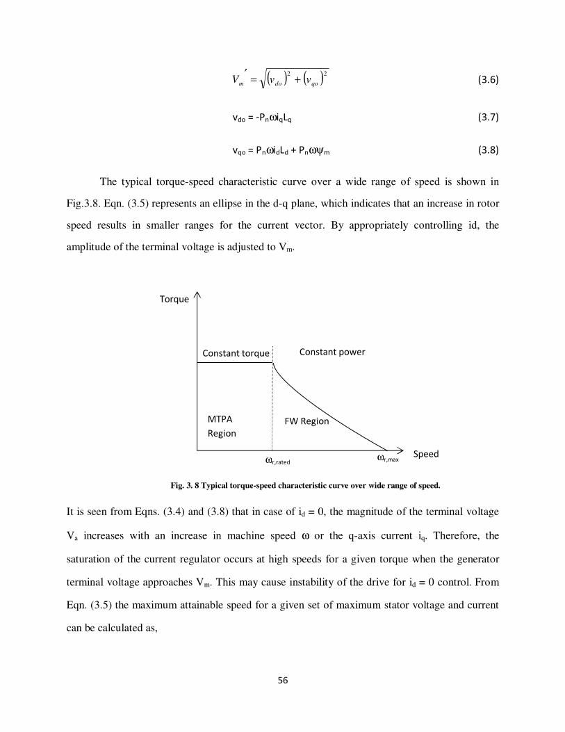
56
( ) ( )22
qodom vvV +=′
(3.6)
vdo = -PnωiqLq (3.7)
vqo = PnωidLd + Pnωψm (3.8)
The typical torque-speed characteristic curve over a wide range of speed is shown in
Fig.3.8. Eqn. (3.5) represents an ellipse in the d-q plane, which indicates that an increase in rotor
speed results in smaller ranges for the current vector. By appropriately controlling id, the
amplitude of the terminal voltage is adjusted to Vm.
It is seen from Eqns. (3.4) and (3.8) that in case of id = 0, the magnitude of the terminal voltage
Va increases with an increase in machine speed ω or the q-axis current iq. Therefore, the
saturation of the current regulator occurs at high speeds for a given torque when the generator
terminal voltage approaches Vm. This may cause instability of the drive for id = 0 control. From
Eqn. (3.5) the maximum attainable speed for a given set of maximum stator voltage and current
can be calculated as,
Speed
Torque
ωr,rated ωr,max
MTPA
Region
FW Region
Constant torque Constant power
Fig. 3. 8 Typical torque-speed characteristic curve over wide range of speed.
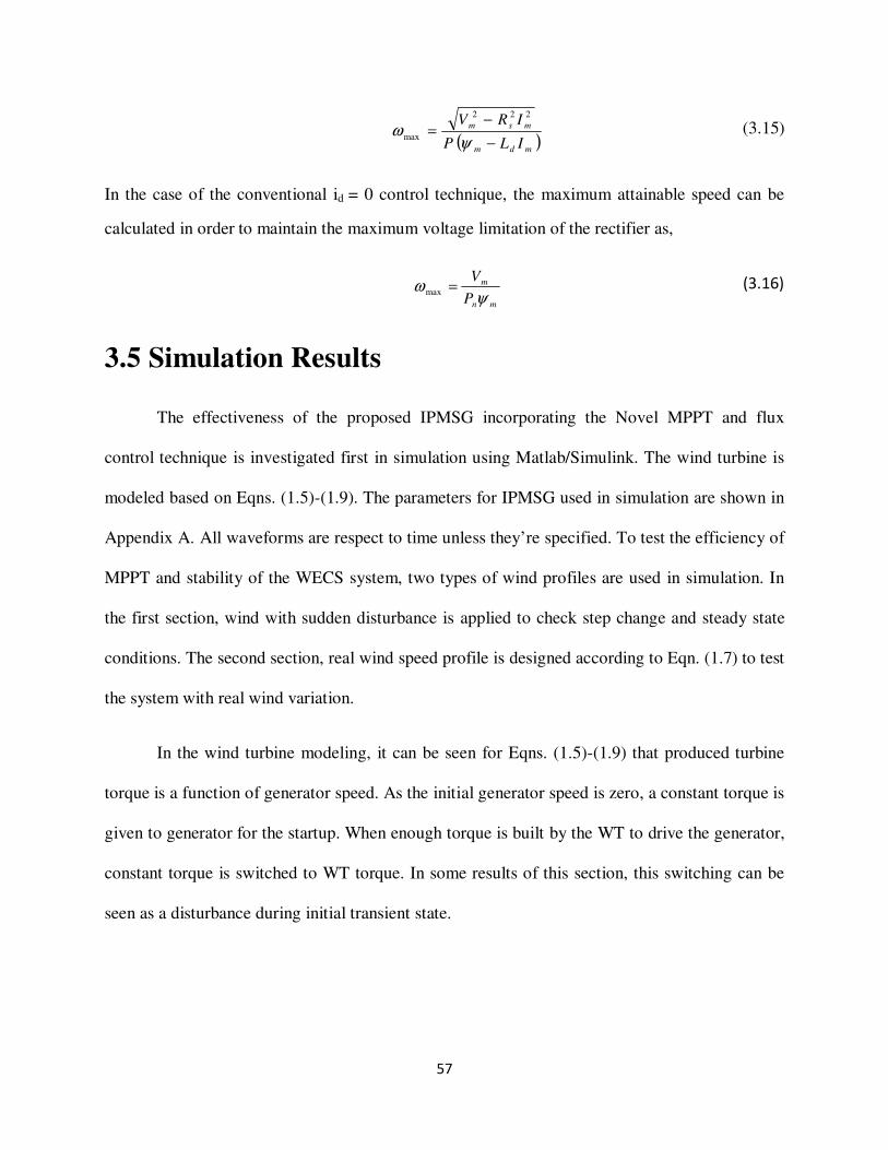
57
( )mdm
msm
ILP
IRV
−
−=
ψω
222
max (3.15)
In the case of the conventional id = 0 control technique, the maximum attainable speed can be
calculated in order to maintain the maximum voltage limitation of the rectifier as,
mn
m
P
V
ψω =max
(3.16)
3.5 Simulation Results
The effectiveness of the proposed IPMSG incorporating the Novel MPPT and flux
control technique is investigated first in simulation using Matlab/Simulink. The wind turbine is
modeled based on Eqns. (1.5)-(1.9). The parameters for IPMSG used in simulation are shown in
Appendix A. All waveforms are respect to time unless they’re specified. To test the efficiency of
MPPT and stability of the WECS system, two types of wind profiles are used in simulation. In
the first section, wind with sudden disturbance is applied to check step change and steady state
conditions. The second section, real wind speed profile is designed according to Eqn. (1.7) to test
the system with real wind variation.
In the wind turbine modeling, it can be seen for Eqns. (1.5)-(1.9) that produced turbine
torque is a function of generator speed. As the initial generator speed is zero, a constant torque is
given to generator for the startup. When enough torque is built by the WT to drive the generator,
constant torque is switched to WT torque. In some results of this section, this switching can be
seen as a disturbance during initial transient state.
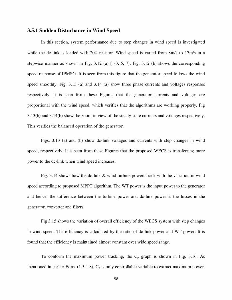
58
3.5.1 Sudden Disturbance in Wind Speed
In this section, system performance due to step changes in wind speed is investigated
while the dc-link is loaded with 20 resistor. Wind speed is varied from 8m/s to 17m/s in a
stepwise manner as shown in Fig. 3.12 (a) [1-3, 5, 7]. Fig. 3.12 (b) shows the corresponding
speed response of IPMSG. It is seen from this figure that the generator speed follows the wind
speed smoothly. Fig. 3.13 (a) and 3.14 (a) show three phase currents and voltages responses
respectively. It is seen from these Figures that the generator currents and voltages are
proportional with the wind speed, which verifies that the algorithms are working properly. Fig
3.13(b) and 3.14(b) show the zoom-in view of the steady-state currents and voltages respectively.
This verifies the balanced operation of the generator.
Figs. 3.13 (a) and (b) show dc-link voltages and currents with step changes in wind
speed, respectively. It is seen from these Figures that the proposed WECS is transferring more
power to the dc-link when wind speed increases.
Fig. 3.14 shows how the dc-link & wind turbine powers track with the variation in wind
speed according to proposed MPPT algorithm. The WT power is the input power to the generator
and hence, the difference between the turbine power and dc-link power is the losses in the
generator, converter and filters.
Fig 3.15 shows the variation of overall efficiency of the WECS system with step changes
in wind speed. The efficiency is calculated by the ratio of dc-link power and WT power. It is
found that the efficiency is maintained almost constant over wide speed range.
To conform the maximum power tracking, the Cp graph is shown in Fig. 3.16. As
mentioned in earlier Eqns. (1.5-1.8), Cp is only controllable variable to extract maximum power.

59
The maximum Cp that can be achieved by proposed system is 0.465. The simulation results
verify the analytical results shown in Fig. 3.1. Thus, the proposed WECS ensures the extraction
maximum power from wind to the turbine output.
Fig. 3.17 shows the tracking of the power coefficient (Cp) with variation in TSR
corresponding to changes in wind speed. It is clearly seen that the controller is tracking the Cp so
that it can extract maximum power with step changes in wind speed. Thus, the Cp value was
maintained constant. At different speed which was shown in Fig. 3.16.
Fig. 3.18 shows the tracking of dc-link power at different rotor speeds according to
MPPT algorithm. It is clearly seen that the algorithm can track the maximum power condition
almost smoothly. Thus, the algorithm ensures the stability of the overall WECS while tacking the
maximum power transfer from turbine to dc-link. Furthermore, it verifies the analytical results
shown in Fig. 3.2.
It can be seen from Fig. 3.19 that both the turbine power and dc-link power for the
proposed control system is higher than those of the conventional controller based WECS. Thus,
it verifies the effectiveness of transfer more power to the dc-link and power from wind
especially, at high wind speed condition.
Fig 3.20 shows the variation in Cp for conventional control scheme. It is found that the
conventional control cannot maintain Cp constant at different wind speeds, whereas the proposed
control can maintain constant Cp corresponding maximum power extraction as shown in Fig 3.16
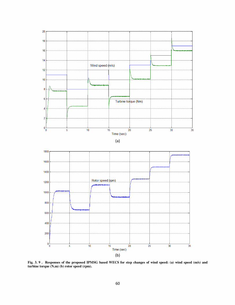
60
(a)
(b)
Fig. 3. 9 . Responses of the proposed IPMSG based WECS for step changes of wind speed: (a) wind speed (m/s) and turbine torque (N.m) (b) rotor speed (rpm).
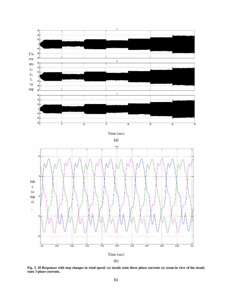
61
(a)
(b)
Fig. 3. 10 Responses with step changes in wind speed: (a) steady state three phase currents (a) zoom-in view of the steady state 3 phase currents.
Time (sec)
Time (sec)
Cu
rre
nts
ia,
ib,
ic
(a
mp
s)
Iab
c
(a
mp
s)
(a
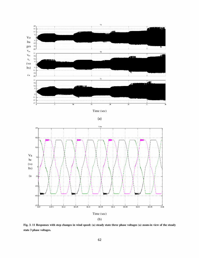
62
(a)
(b)
Fig. 3. 11 Responses with step changes in wind speed: (a) steady state three phase voltages (a) zoom-in view of the steady
state 3 phase voltages.
Time (sec)
Time (sec)
Vo
lta
ges
va,
vb,
vc
(vo
lts)
(a
Va
bc
(vo
lts)
(a
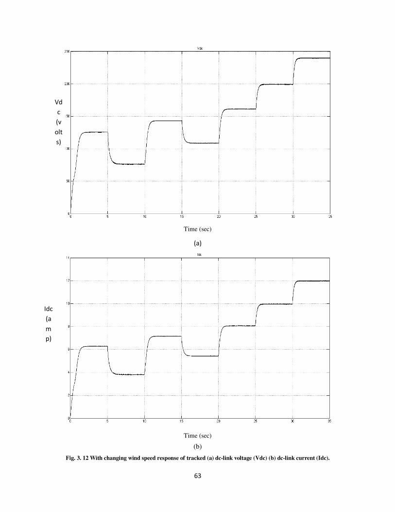
63
(a)
(b)
Fig. 3. 12 With changing wind speed response of tracked (a) dc-link voltage (Vdc) (b) dc-link current (Idc).
Time (sec)
Time (sec)
Vd
c
(v
olt
s)
Idc
(a
m
p)
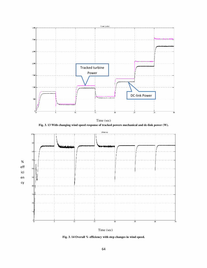
64
Fig. 3. 13 With changing wind speed response of tracked powers mechanical and dc-link power (W).
Fig. 3. 14 Overall % efficiency with step changes in wind speed.
Tracked turbine
Power
DC-link Power
Time (sec)
Time (sec)
%
eff
ici
en
cy
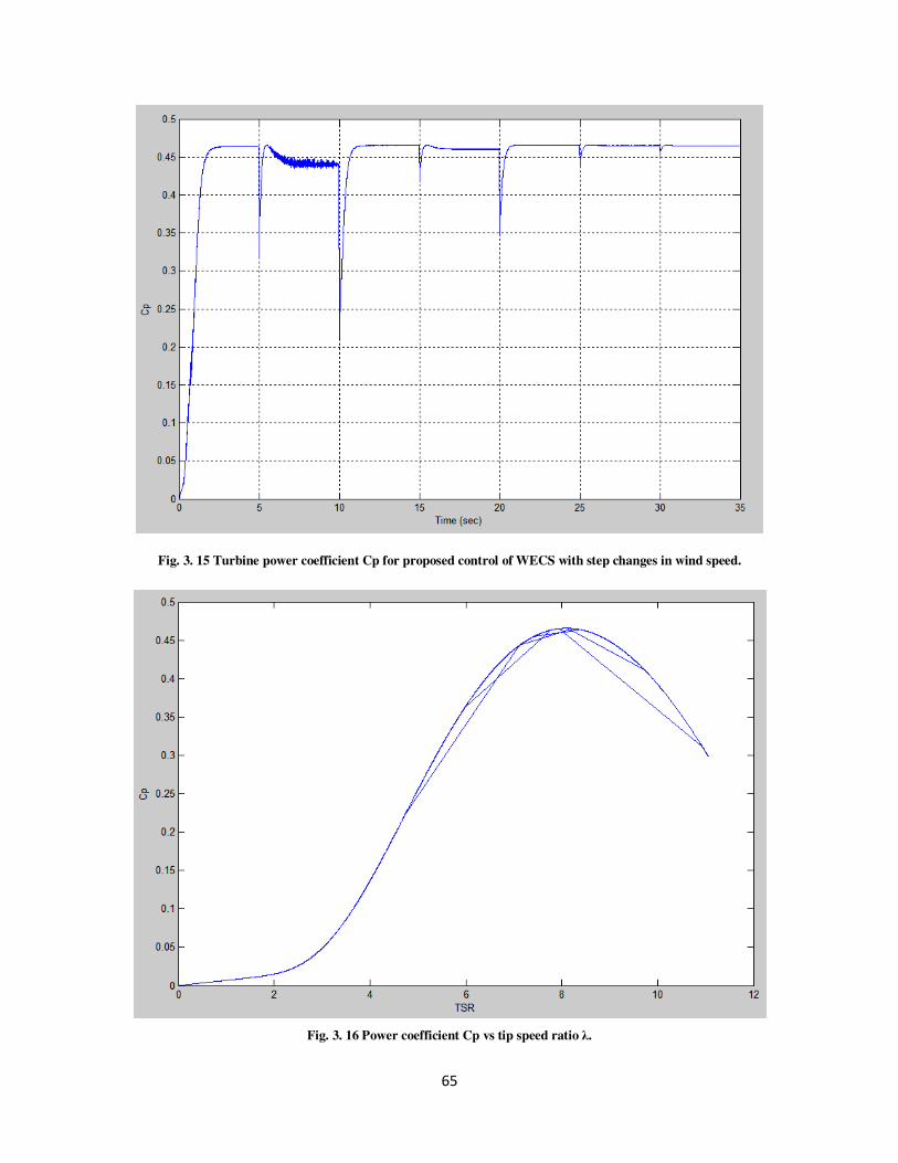
65
Fig. 3. 15 Turbine power coefficient Cp for proposed control of WECS with step changes in wind speed.
Fig. 3. 16 Power coefficient Cp vs tip speed ratio λ.
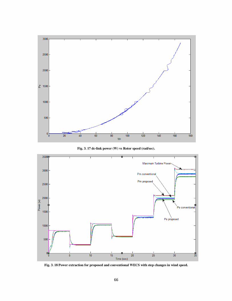
66
Fig. 3. 17 dc-link power (W) vs Rotor speed (rad/sec).
Fig. 3. 18 Power extraction for proposed and conventional WECS with step changes in wind speed.
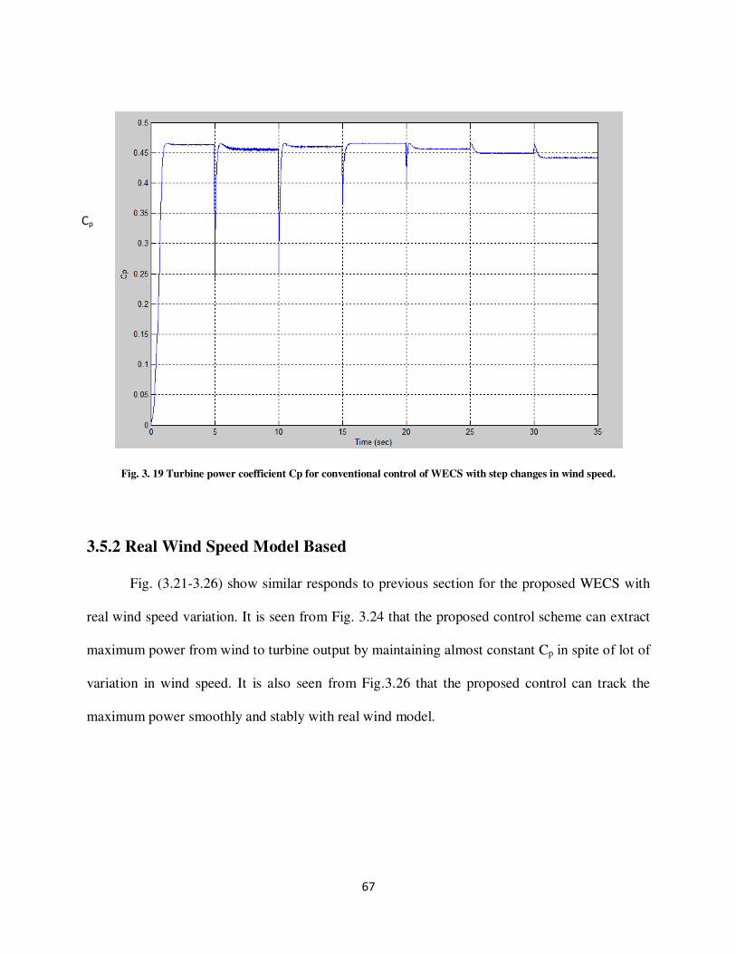
67
Fig. 3. 19 Turbine power coefficient Cp for conventional control of WECS with step changes in wind speed.
3.5.2 Real Wind Speed Model Based
Fig. (3.21-3.26) show similar responds to previous section for the proposed WECS with
real wind speed variation. It is seen from Fig. 3.24 that the proposed control scheme can extract
maximum power from wind to turbine output by maintaining almost constant Cp in spite of lot of
variation in wind speed. It is also seen from Fig.3.26 that the proposed control can track the
maximum power smoothly and stably with real wind model.
Cp
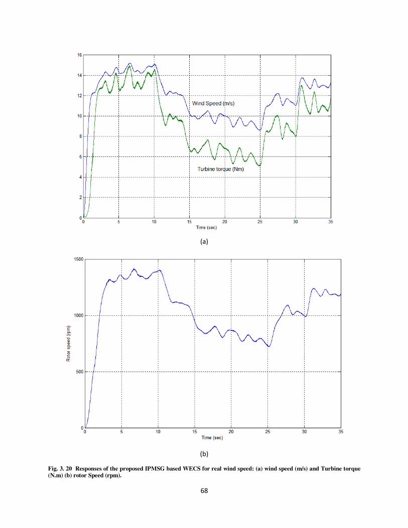
68
(a)
(b)
Fig. 3. 20 Responses of the proposed IPMSG based WECS for real wind speed: (a) wind speed (m/s) and Turbine torque (N.m) (b) rotor Speed (rpm).
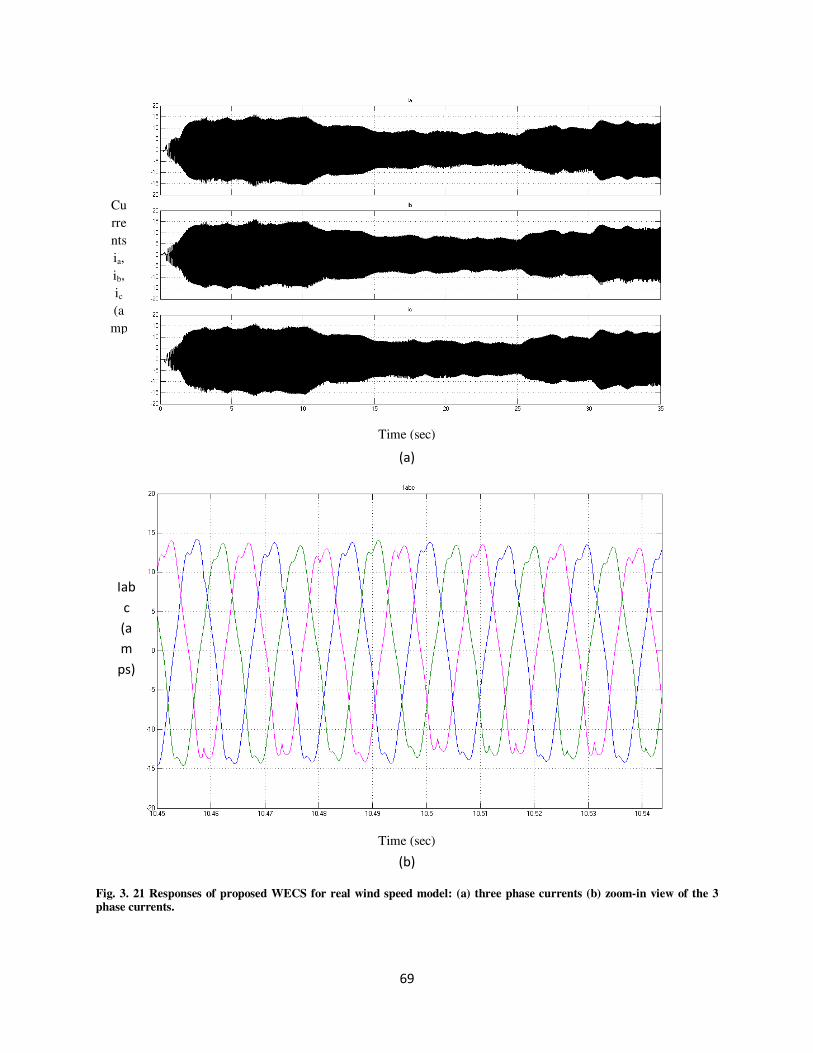
69
(a)
(b)
Fig. 3. 21 Responses of proposed WECS for real wind speed model: (a) three phase currents (b) zoom-in view of the 3 phase currents.
Time (sec)
Time (sec)
Cu
rre
nts
ia,
ib,
ic
(a
mp
Iab
c
(a
m
ps)
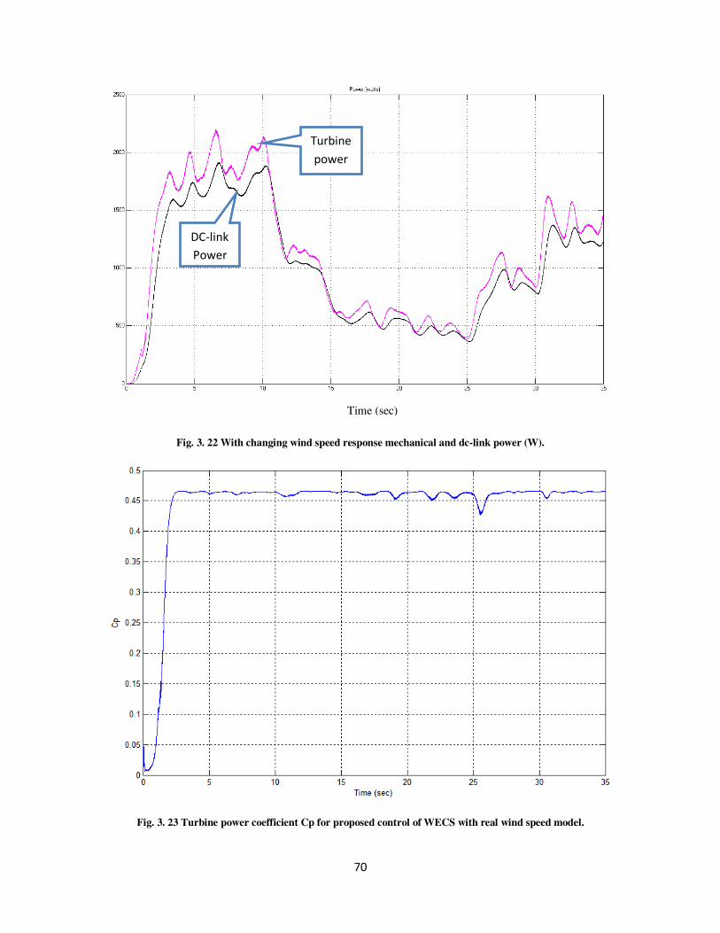
70
Fig. 3. 22 With changing wind speed response mechanical and dc-link power (W).
Fig. 3. 23 Turbine power coefficient Cp for proposed control of WECS with real wind speed model.
Turbine
power
DC-link
Power
Time (sec)
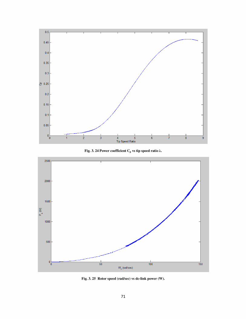
71
Fig. 3. 24 Power coefficient Cp vs tip speed ratio λ.
Fig. 3. 25 Rotor speed (rad/sec) vs dc-link power (W).
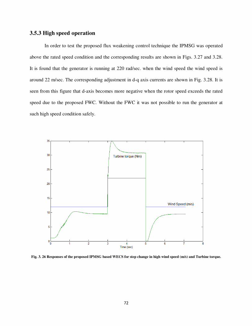
72
3.5.3 High speed operation
In order to test the proposed flux weakening control technique the IPMSG was operated
above the rated speed condition and the corresponding results are shown in Figs. 3.27 and 3.28.
It is found that the generator is running at 220 rad/sec. when the wind speed the wind speed is
around 22 m/sec. The corresponding adjustment in d-q axis currents are shown in Fig. 3.28. It is
seen from this figure that d-axis becomes more negative when the rotor speed exceeds the rated
speed due to the proposed FWC. Without the FWC it was not possible to run the generator at
such high speed condition safely.
Fig. 3. 26 Responses of the proposed IPMSG based WECS for step change in high wind speed (m/s) and Turbine torque.
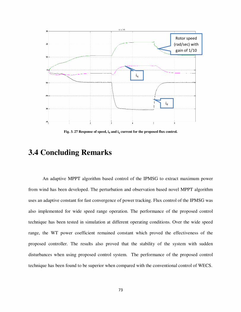
73
Fig. 3. 27 Response of speed, id and iq current for the proposed flux control.
3.4 Concluding Remarks
An adaptive MPPT algorithm based control of the IPMSG to extract maximum power
from wind has been developed. The perturbation and observation based novel MPPT algorithm
uses an adaptive constant for fast convergence of power tracking. Flux control of the IPMSG was
also implemented for wide speed range operation. The performance of the proposed control
technique has been tested in simulation at different operating conditions. Over the wide speed
range, the WT power coefficient remained constant which proved the effectiveness of the
proposed controller. The results also proved that the stability of the system with sudden
disturbances when using proposed control system. The performance of the proposed control
technique has been found to be superior when compared with the conventional control of WECS.
id
Rotor speed
(rad/sec) with
gain of 1/10
iq

74
Chapter 4
Sensorless Control- Position and Speed
Estimation
4.1 Introduction
Speed sensorless control means that the rotor position is not measured by encoder, but
estimated online using some algorithms. However, their control still uses some basic sensors, e.g.
current sensors, voltage sensors. In recent decade, much research has been done in the area of
speed and/ or shaft position sensorless controlled drives [59-83].
The main drawback of a PM-machine is the position sensor, which is vulnerable for
electromagnetic noise in hostile environments and has a limited temperature range. For PM
machines rated up to 10kW the cost of an encoder is below 10% of the machine manufacturing
cost. However, for applications in the automotive industry with the elimination of the position
sensor is preferable due to space limitation and cost. Thus, the elimination of the
electromechanical sensors reduces the hardware costs, reduces the installation complexity of the
system (because of associated wiring), decreases the system inertia, increases the robustness and
the reliability and reduces obviously the noise sensitivity of the electrical drive [2],[3].

75
4.2 Strategies for Position and Speed Estimation for
IPMSM
In general there are three strategies for position estimation of IPMSM [60], [61]:
1. Model based estimators,
2. Saliency and Signal Injection,
3. Artificial Intelligence.
1. Model based estimators:
The method uses the model of the PM machine and measured electrical quantities
to determine the rotor position and speed. The measured electrical quantity is usually the stator
current of the PM machine. This method is further classified into two types such as, (a) non-
adaptive and (b) adaptive methods.
a) Non-adaptive Methods are divided in the following three categories:
i. Techniques using the measured dc-link current assuming constant dc-link voltage,
ii. Estimators using monitored stator voltages, or currents,
iii. Flux based position estimators,
iv. Position estimators based on back-EMF.
b) Adaptive Methods are divided into the following four categories:
i. Estimator based on Model Reference Adaptive System (MRAS).
ii. Observer-based estimators.
iii. Kalman filter based estimator.

76
iv. Estimator which use the minimum error square.
2. Saliency and Signal Injection:
In PM machines, the position dependence is a feature of the rotor. In the case of the
interior PMSM there is a measurably spatial variation of inductances or resistances (saliencies)
in the d-q direction due to geometrical and saturation effects, which can be used for the
estimation of rotor position . In this method, an additional signal (voltage or current) is injected
into the machine and the position angle and speed are determined by processing the returning
currents or voltages. Based on the signal injection, this method is further divided into the
following two groups.
(a) High Frequency Method:
In this estimation of the rotor position, high frequency stator voltage (current) component
is added to machine and the effects of the machine saliency (anisotropy) is evaluated on the
amplitude of the correspondent stator voltage (current) component. In the literature the
frequency of the injection signal is from a few hundred Hz to KHz region.
(b) Low Frequency Method:
This estimators are based on the mechanical vibration of the rotor. The injected frequency
is usually from few Hz to few hundred Hz.
3. Artificial Intelligence:
Artificial intelligence methods use neural network, fuzzy logic based systems or neuro –
fuzzy systems to estimate the rotor position. These kind of methods do not require a
mathematical model of the drive, exhibit good noise rejection properties, can easily be extended
and modified, can be robust to parameter variations and are computationally less intensive.

77
Fuzzy logic estimators are based on linguistic rules determined by experts. Neural
network estimators learn the properties of the particular machine using predetermined training
data. The inputs of the neural network are currents and voltages. Neuro-fuzzy technique has an
advantage of fuzzy logic and neural network which has self-learning, self-organizing and self-
tuning capabilities.
These techniques require high bandwidth and high precision measurement, and fast signal
processing capability, which may increase the complexity and cost of control system. The
injected high-frequency voltages may also cause more torque ripple, shaft vibration and audible
noises. On the other hand, MRAS scheme offer simpler implementation and require less
computational effort compared to other methods, and it is widely accepted for speed estimation.
Mathematical model of MRAS is discussed in following section.
4.2 Model Reference Adaptive System Based Speed
Estimation
The model reference adaptive system includes two models: the reference model and the
adaptive model. The external excitation for the two models is the same, and the difference state
vector between the outputs of the two models is used as the input of adaptive unit. Based on this
input the parameters of the adaptive model should be modified so that the output state vector of
the adaptive model approaches toward the reference model fast and stably. For the current of
PMSG can be directly measured, current model of PMSG is usually used as adjustable model. In

78
d-q reference frame, the mathematical model of IPMSM Eqns. (2.18-2.19) can be rewritten in
current model form as:
−+
−−
−
=
q
mq
d
d
q
d
q
s
q
d
d
q
d
s
q
d
L
v
L
v
i
i
L
R
L
L
L
L
L
R
i
ip ωψ
ω
ω
(4.1)
Where p is derivative operator. Eqn. (4.1) can be rewritten as [12],
+
+
+
−
−−
=
+
q
q
d
msdd
q
d
m
d
q
s
q
d
d
q
d
s
q
d
m
d
L
v
L
RLv
i
Li
L
R
L
L
L
L
L
R
i
Li
p
2
ψψ
ω
ωψ
(4.2)
Let’s assume,
+
=
=
q
d
m
d
i
Li
x
xx
ψ
2
1
−
−−
=
q
s
q
d
d
q
d
s
L
R
L
L
L
L
L
R
A
ω
ω
+
=
q
q
d
msdd
L
v
L
RLv
u
2
ψ
The state Eqn. (4.2) would be
uAxpx += (4.3)

79
So the adaptive model can be written as,
uxAxp +=^^^
4.4)
Where,
−
−−
=
q
s
q
d
d
q
d
s
L
R
L
L
L
L
L
R
A^
^
^
ω
ω
Now suppose error vector is given by,
+
=
−
−=−=
q
d
m
d
i
Li
xx
xxxxe
ψ
^
22
^
11^
(4.5)
From Eqns. (4.3)(4.4), there would be,
HAepe −= (4.6)
And in Eqn. (4.6),
^^
0
0
)( x
L
L
L
L
H
q
d
d
q
−
=−= ωω
According to Popov’s hyperstability criterion [100], the adaptive law could be obtained as:
)0()()(^
21
^
ωτω ++= ∫ dNCNC (4.8)
∫= τωθ d)(^^
(4.9)
80
Where,
−−+
−
+−= ddq
d
qqq
d
md
q
d iiiL
Lii
Li
L
LN
^^^^ ψ, )0(
^
ω is initial speed and C1,C2 are
proportional and integral gains respectively.
Eqn (4.8) represents a PI controller. Thus, the error between reference and adaptive
model is processed through the PI controller, which gives the estimated speed as output.
The estimating performance of rotor speed is designed only by the PI coefficients. The
proposed SVPWM using MRAS-based speed estimation for sensorless MPPT control of IPMSG
drive was shown in Fig. 3.7.
4.3 Simulation Results
The complete simulation model for the proposed sensorless MPPT and flux controller
based WECS is built in Matlab/simulink. The generator parameters are given in appendix A.
Simulation blocks are shown in Appendix B. Estimation of rotor speed and position is achieved
for IPMSG with 3 pole pairs. Fig 4.1(a) shows the rotor position estimation and phase ‘a’ current
during steady state, whereas Fig. 4.1(b) shows the rotor position estimation and phase ‘a’ current
during step change in wind speed. The angle in both these figures corresponds to electrical
frequency of generator and has maximum amplitude of 2π rad for each cycle which confirms the
accuracy and stability of the rotor position estimation.
Fig 4.2(a) and 4.2 (b) shows the comparative measured and estimated rotor speed for real
wind profile and step changes in wind, respectively. It is clearly seen that the estimated speed is
same as the measured rotor speed for both wind speed disturbances. The corresponding speed
estimation errors are shown in Fig. 4.3 (a) and 4.2(a) for both wind speed profiles. As the wind
speed was changed from very low to high as shown in Fig. 3.11(a), the high accuracy has been
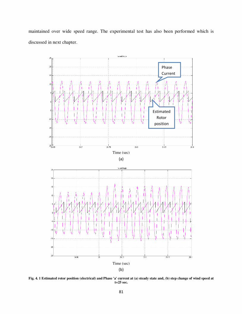
81
maintained over wide speed range. The experimental test has also been performed which is
discussed in next chapter.
(a)
(b)
Fig. 4. 1 Estimated rotor position (electrical) and Phase 'a' current at (a) steady state and, (b) step change of wind speed at t=25 sec.
Phase
Current
Estimated
Rotor
position
Time (sec)
Time (sec)
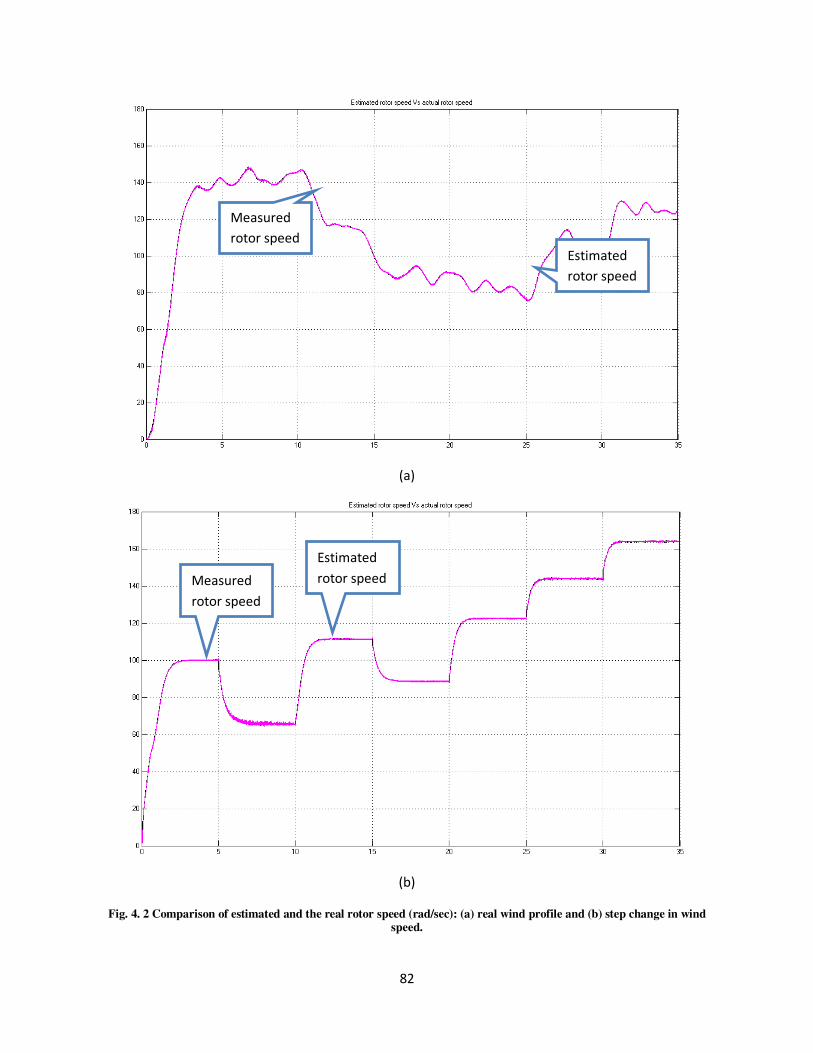
82
(a)
(b)
Fig. 4. 2 Comparison of estimated and the real rotor speed (rad/sec): (a) real wind profile and (b) step change in wind speed.
Measured
rotor speed
Estimated
rotor speed
Estimated
rotor speed
Measured
rotor speed
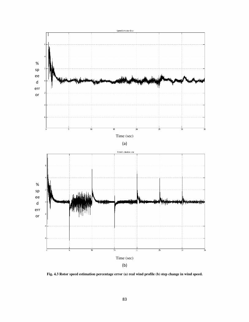
83
(a)
(b)
Fig. 4.3 Rotor speed estimation percentage error (a) real wind profile (b) step change in wind speed.
Time (sec)
Time (sec)
%
sp
ee
d
err
or
%
sp
ee
d
err
or

84
4.4 Concluding Remarks
The MRAS based speed and position estimations have been proposed in this Chapter. As
compared to the others, the proposed MRAS technique is relatively simple and therefore, has low
computational burden. The results proved the effectiveness of position estimation in both steady-
state and transient conditions. It has also been found from results that the proposed MRAS tracks
the rotor speed without significant error at variable wind speed conditions. The simulation results
showed that the speed estimation error was maintained below +2% at different rotor speeds. The
real-time implementation of the proposed MPPT and MRAS based speed and position estimation
techniques for IPMSG based WECS is shown in Chapter 5.

85
Chapter 5
Real-time Implementation
5.1 Introduction
The performance of the proposed drive was tested in real-time after getting some
promising results in simulation. The complete sensorless vector control scheme of IPMSG
incorporating the proposed MPPT based algorithm is successfully implemented in real-time
using DSP board controller board DS 1104. The dSPACE DS1104 board is a very flexible and
powerful system both for high computational capability and comprehensive I/O periphery. The
detailed real-time implementation is described in this chapter.
5.2 Experimental Setup
The experimental setup for the prototype 5 HP IPMSG based WECS is shown in Fig. 5.1
and 5.2. The test IPMSG is labelled as 'G'. The rotor speed of the test machine is measured by an
optical incremental encoder which is labelled as 'E'. The measured speed is only used for
comparison purpose with the estimated rotor speed. The encoder is directly connected to the
rotor shaft. The IPMSG is coupled with a PM-DC machine (M), which works as a separately
excited motor to drive the generator. Thus, the DC motor replaces the wind turbine in a
laboratory environment. The actual motor currents are measured by Hall-effect current
transducers.
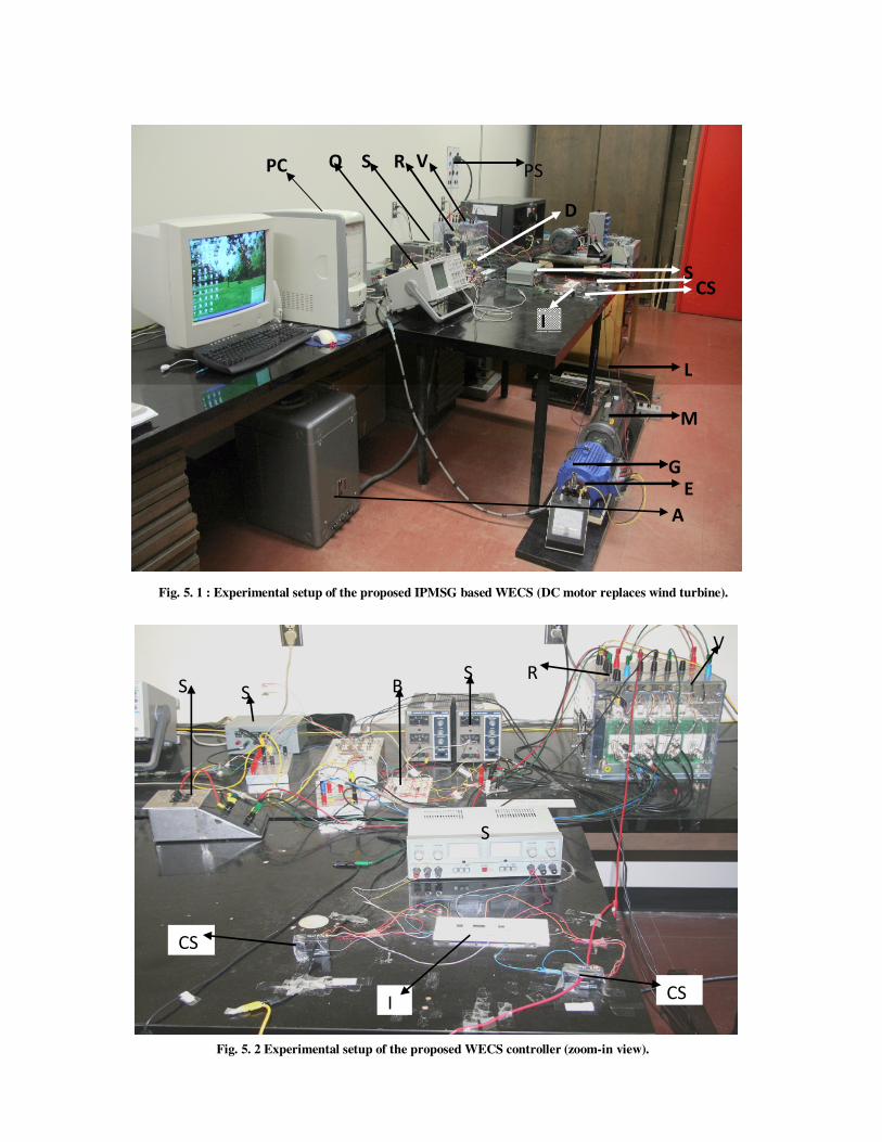
86
G
E
M
L
CS S
A
V O S R PC
D
I
PS
S
S S
CS
CS
R
V
B S
I
Fig. 5. 1 : Experimental setup of the proposed IPMSG based WECS (DC motor replaces wind turbine).
Fig. 5. 2 Experimental setup of the proposed WECS controller (zoom-in view).

87
The interface circuit (I) is located between the Hall-effect sensor and the A/D channel of
DSP board. These transducers are labelled as 'CS'. These current sensors (CS) have a linear
response over wide range of frequencies (up to 250 kHz). Another gate drive circuit is used to
increase the power level of the firing pulses so that these are sufficient to drive the converter
insulated gate bipolar transistor (IGBT) switches. The gate drive circuit also provides isolation
between low power control and the high power supply circuits. The gate drive circuit is labelled
as 'D'. The power circuits consist of a 3-phase variable ac autotransformer (A), power supply
(PS), rectifier (R) and IGBT converter (V). The ac voltage is supplied by the power supply
through autotransformer which is rectified by uncontrolled rectifier to supply DC motor. The
speed of the motor is changed by varying the input ac voltage to the rectifier. Thus, it simulates
the variable wind speed conditions. The rectifier enclosed within 3-phase (6 pulses) IGBT
converter is labelled as 'V'. This converter has active security feature against short circuit, under
voltage of power
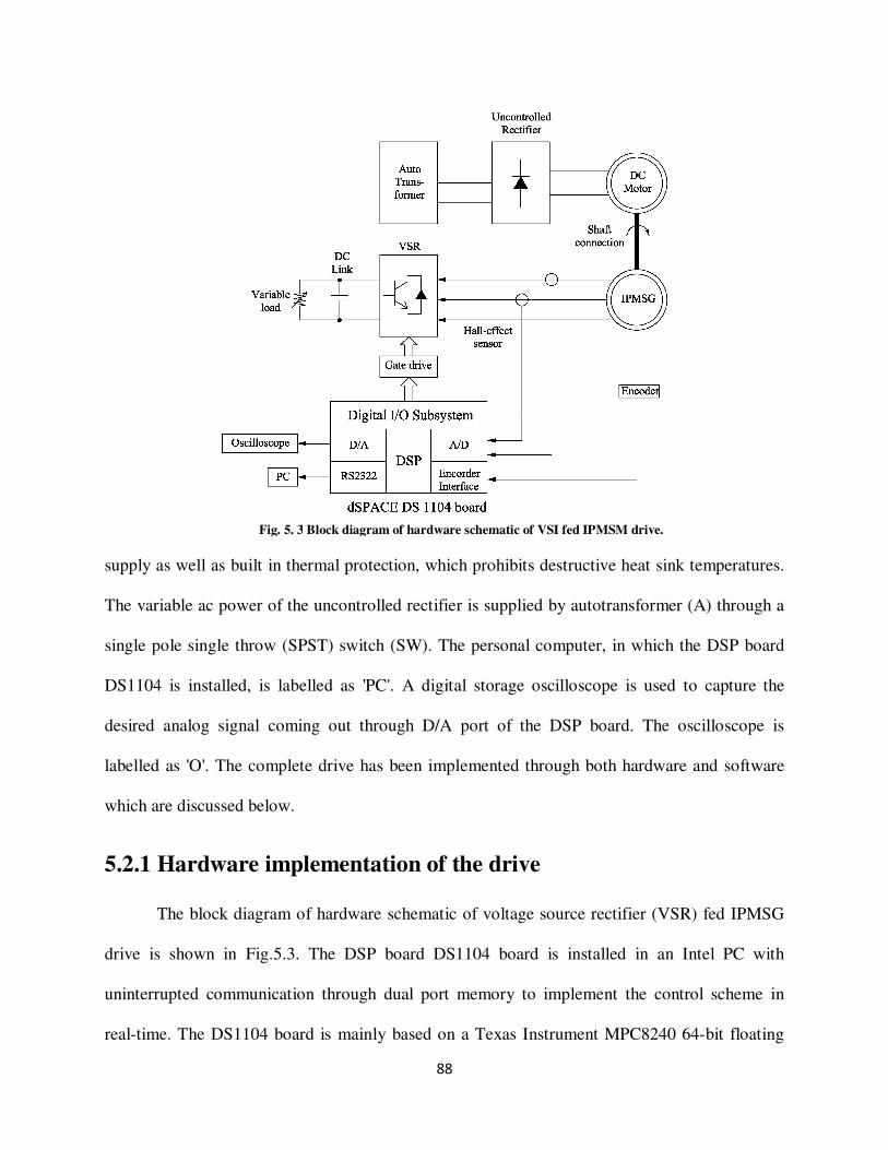
88
supply as well as built in thermal protection, which prohibits destructive heat sink temperatures.
The variable ac power of the uncontrolled rectifier is supplied by autotransformer (A) through a
single pole single throw (SPST) switch (SW). The personal computer, in which the DSP board
DS1104 is installed, is labelled as 'PC'. A digital storage oscilloscope is used to capture the
desired analog signal coming out through D/A port of the DSP board. The oscilloscope is
labelled as 'O'. The complete drive has been implemented through both hardware and software
which are discussed below.
5.2.1 Hardware implementation of the drive
The block diagram of hardware schematic of voltage source rectifier (VSR) fed IPMSG
drive is shown in Fig.5.3. The DSP board DS1104 board is installed in an Intel PC with
uninterrupted communication through dual port memory to implement the control scheme in
real-time. The DS1104 board is mainly based on a Texas Instrument MPC8240 64-bit floating
Fig. 5. 3 Block diagram of hardware schematic of VSI fed IPMSM drive.

89
point digital signal processor. The block diagram of the DSP board is shown in Fig.5.4. The
DS1104 board uses a PowerPC type PPC603e processor which operates at the clock of 250 MHz
with 32 KB cache. This board has a 32 MB of SDRAM global memory and 8 MB of flash
memory. The DSP is supplemented by a set of on-board peripherals used in digital control
systems including analog to digital (A/D), digital to analog (D/A) converters and digital
incremental encoder interfaces. This board is also equipped with a TI TMS320F240 16-bit micro
controller DSP that acts as a slave processor and provides the necessary digital I/O ports
configuration and powerful timer functions such as input capture, output capture and PWM
generation. In this work, the slave processor is used for only digital I/O subsystem configuration.
The block diagram of the hardware schematic is shown in Fig. 5.3. Rotor position is sensed by an
optical incremental encoder mounted at the rotor shaft and is fed back to the DSP board through
the encoder interface. The encoder used in this work generates 1024 pulses per revolution. By
using a built-in 4-fold pulse multiplication the output of the encoder is increased to 4x1024
pulses per revolution in order to get a better resolution. So the resolution of the encoder is
0.087890625°. These pulses are fed to the one of two digital incremental encoder interface
channels of the board. A 24-bit position counter is used to count the encoder pulses and is read
by a calling function in the software. The counter is reset in each revolution by the index pulse
generated from the encoder. The generator speed is computed from the measured rotor position
angles using discrete difference equation. The measured speed is used to compare estimated
speed. The actual generator currents are measured by the Hall-effect sensors, which have current
range of 0 ~ ±200A and a frequency range of 0~250 KHz. The current signals are fed back to
DSP board through A/D channels. The output current signal of these sensors is converted to a
voltage across the resistor connected between the output terminal of the sensor and ground. One
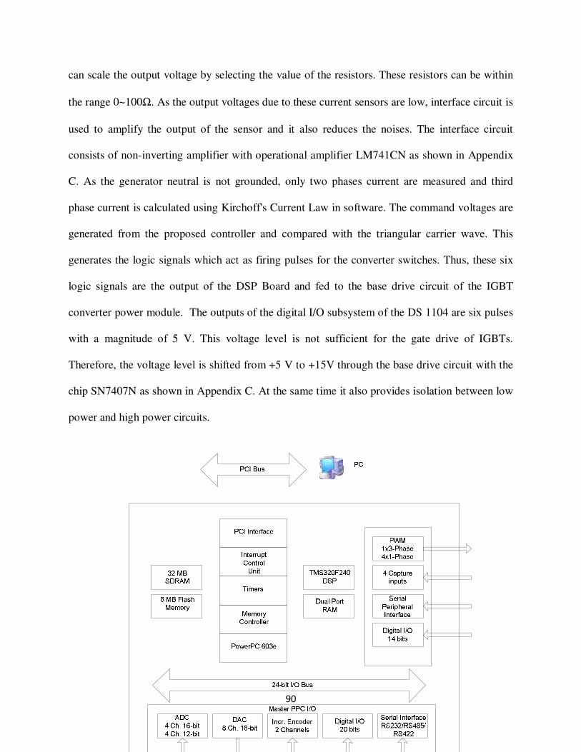
90
can scale the output voltage by selecting the value of the resistors. These resistors can be within
the range 0~100Ω. As the output voltages due to these current sensors are low, interface circuit is
used to amplify the output of the sensor and it also reduces the noises. The interface circuit
consists of non-inverting amplifier with operational amplifier LM741CN as shown in Appendix
C. As the generator neutral is not grounded, only two phases current are measured and third
phase current is calculated using Kirchoff's Current Law in software. The command voltages are
generated from the proposed controller and compared with the triangular carrier wave. This
generates the logic signals which act as firing pulses for the converter switches. Thus, these six
logic signals are the output of the DSP Board and fed to the base drive circuit of the IGBT
converter power module. The outputs of the digital I/O subsystem of the DS 1104 are six pulses
with a magnitude of 5 V. This voltage level is not sufficient for the gate drive of IGBTs.
Therefore, the voltage level is shifted from +5 V to +15V through the base drive circuit with the
chip SN7407N as shown in Appendix C. At the same time it also provides isolation between low
power and high power circuits.

91
Fig. 5. 4 Block diagram of DS1104 board.
5.3.2 Software implementation of the drive
The dSPACE DS1104 board is a self-contained system, not an embedded system. This
means the board installed in the lab computer through a PCI slot is its own entity and the host PC
does none of the processing for a system implemented on the board. As a result, the board
requires that software to be created and downloaded to the board for the system to function.
The ControlDesk software is used to download software to the DSP board, start and stop
the function of the DS1104 as well as create a layout for interfacing with global variables in
dSPACE programs. The sampling frequency used in this work is found to be 5 kHz. If the
sampling frequency that is higher than 5 kHz is chosen, the 'overrun error' occurs, which
indicates too much computational burden for the processor. The simulink blocks used for real-
time implementations is shown in Appendix D.
5.3 Experimental Results
In order to verify the effectiveness and the dynamic performances of the proposed
sensorless MPPT control of IPMSG based WECS, experimental tests have been carried out.
Sample results are presented below. Fig. 5.5 illustrates the rotor position estimation using MRAS

92
model. As the IPMSG is 3 pole pair machine, one cycle of rotor position angle corresponds to
three cycle of phase ‘a’ current. Fig. 5.6 shows the performance of the MRAS observer tracking
the rotational speed under various speed conditions. It can be observed that the estimated speed
tracks the actual rotor speed very well and the estimation error is very small during the transient
state. Thus, the effectiveness of the proposed speed sensorless scheme is verified. Fig. 5.7 shows
three phase output voltages and currents of IPMSG under fixed speed condition. The voltage and
current waveform validate the balanced operation of the system.
To conform the maximum power point tracking control, couple of experimental tests
have been carried out. As the IPMSG is driven by 5 HP DC machine, the WT parameter is
unavailable for conventional controller. For this reason, the testing using conventional control is
not available. This is also the main drawback of conventional controller that it requires WT
information.
Fig. 5. 5 Phase 'a' current and estimated rotor position angle.
Phase current
(amp)
Estimated rotor
angle (rad)
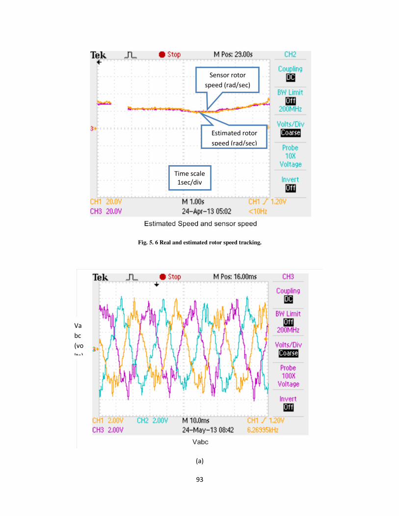
93
Fig. 5. 6 Real and estimated rotor speed tracking.
(a)
Sensor rotor
speed (rad/sec)
Estimated rotor
speed (rad/sec)
Time scale
1sec/div
Va
bc
(vo
lts)
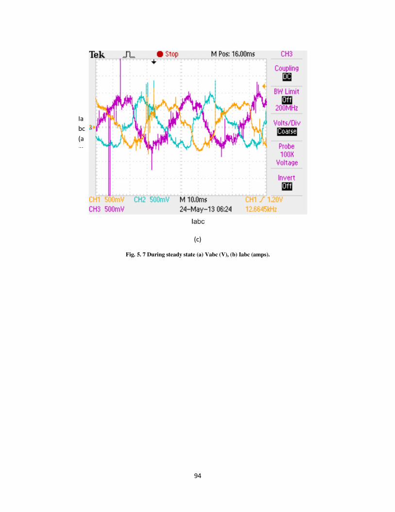
94
(c)
Fig. 5. 7 During steady state (a) Vabc (V), (b) Iabc (amps).
Ia
bc
(a
m
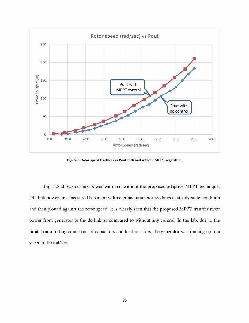
95
Fig. 5. 8 Rotor speed (rad/sec) vs Pout with and without MPPT algorithm.
Fig. 5.8 shows dc-link power with and without the proposed adaptive MPPT technique.
DC-link power first measured based on voltmeter and ammeter readings at steady-state condition
and then plotted against the rotor speed. It is clearly seen that the proposed MPPT transfer more
power from generator to the dc-link as compared to without any control. In the lab, due to the
limitation of rating conditions of capacitors and load resistors, the generator was running up to a
speed of 80 rad/sec.
0
50
100
150
200
250
0.0 10.0 20.0 30.0 40.0 50.0 60.0 70.0 80.0 90.0
Po
we
r o
utp
ut
(w)
Rotor Speed (rad/sec)
Rotor speed (rad/sec) vs Pout
Pout with
MPPT control
Pout with
no control

96
5.5 Concluding Remarks
The detailed experimental implementation of the proposed sensorless control of IPMSG
based in MPPT technique using dSPACE DSP board DS1104 has been presented in this Chapter.
The performance of the proposed drive has been tested in real-time at different operating rotor
speed. In order to prove the superiority, the performance of the proposed MPPT based technique
has been compared with a no controller tracking condition. Due to MPPT algorithm extracted
power has been increased. Due to simplicity of MRAS sensorless technique, it was possible to
implement it in real-time. Position estimation comparison with phase current showed the
effectiveness of MRAS technique. Speed estimation has been also tested at various speed
conditions. It was noticed that speed was tracked with minimum speed error.
97
Chapter 6
Conclusions
6.1 Concluding Remarks
An improved control technique for variable-speed WECS using an IPMSG to extract
maximum power over wide operating speed range has been proposed in this thesis. A novel
adaptive MPPT with sensorless scheme have been proposed to maximize generated output
power. Additionally, flux weakening control technique has been also implemented to extend the
operating speed range. The MPPT algorithm generates optimum speed reference to track
maximum power without the knowledge of wind speed, turbine parameter or generator
parameters. The proposed control system incorporated flux weakening controller above rated
speed. In Matlab/Simulink control system was tested with sudden disturbance in wind speed
varying from 8m/s to 17m/s, and maximum power coefficient Cp was maintained almost constant
during wide speed operating range. The proposed controller has also been tested with real wind
speed model which conformed maximum power transfer maintaining high stability and high
controllability of the IPMSG.
A sensorless MPPT control of IPMSG and the SVPWM rectifier has been implemented
in real time using DSP board DS1104. The speed sensorless technique has been developed based
on model reference adaptive system (MRAS) algorithm. In real time, a 5 HP variable speed DC

98
motor has been used to replace the WT. The experimental results verified the effectiveness of
sensorless and MPPT technique for the proposed IPMSG based WECS.
6.2 Future work
During continuous operation of IPMSG, it may increase internal temperature, so online
parameter adaptation technique could be incorporated in the system.
The effect of magnetic saturation, which causes highly non-linear characteristic of the
IPMSG, needs to be considered in control scheme design.
Fuzzy logic controller can be implemented in sensorless MRAS scheme to replace the PI
controller.
Loss minimization technique can be implemented in order to improve the efficiency of
the system
99
References
[1] S. Morimoto, H. Kato, M. Sanada and Y. Takeda, "Output Maximization Control for
Wind Generation System with Interior Permanent Magnet Synchronous Generator", in
41st IAS Annual Meeting IEEE Industry Applications Conference, Tampa, FL, 2006.
[2] S. Morimoto, M. Sanada and Y. Takeda, "Optimum control of IPMSG for wind
generation system", in PCC Osaka Power Conversion Conference, Osaka, 07 August
2002.
[3] J. S. Thongam, P. Bouchard, H. Ezzaidi and M. Ouhrouche, "Wind Speed Sensorless
Maximum Power Point Tracking Control of Variable Speed Wind Energy Conversion
Systems", in IEEE IEMDC, Miami, FL, 3-6 May 2009.
[4] N. Srighakollapu and P. Sensarma, "Sensorless maximum power point tracking control
in wind energy generation using permanent magnet synchronous generator", in 34th
Annual Conference of IEEE Industrial Electronics, Orlando, FL, 10-13 Nov. 2008.
[5] J. S. Thongam, P. Bouchard, R. Beguenane and I. Fofana, "Neural network based wind
speed sensorless MPPT controller for variable speed wind energy conversion systems",
in IEEE Electric Power and Energy Conference, Halifax, NS, Aug 25-27, 2010.
[6] J. S. Thongam, P. Bouchard, R. Beguenane, I. Fofana, and M. Ouhrouche, "Sensorless
Control of PMSG in Variable Speed Wind Energy Conversion Systems", in IPEC 2010,
pp. 2254 - 2259, Sapporo, 21-24 June 2010.
[7] A. M. O. Haruni, M. E. Haque, A. Gargoom and M. Negnevitsky, "Control of a Direct
100
Drive IPM Synchronous Generator Based Variable Speed Wind Turbine with Energy
Storage", IECON 2010 - 36th Annual Conference on IEEE Industrial Electronics
Society, Glendale, AZ, Nov 2010.
[8] V. Quaschning, “Understanding Renewable Energy Systems, London”, UK & Sterling,
VA: Earthscan, 2005.
[9] "2012 Half year report", The World Wind Energy Association, Bonn, Germany,
October, 2012.
[10] A. Merabet, R. Beguenane, J. S. Thongam and I. Hussein, "Adaptive Sliding Mode
Speed Control for Wind Turbine Systems", in 37th Annual Conference on IEEE
Industrial Electronics Society, Melbourne, VIC, 2011.
[11] X. Yang, X. Gong and W. Qiao, "Mechanical sensorless maximum power tracking
control for direct-drive PMSG wind turbines", in IEEE Energy Conversion Congress
and Exposition (ECCE), Atlanta, GA, 2010.
[12] W. Liu, L. Chen, J. Ou and S. Cheng, "Simulation of PMSG wind turbine system with
sensor-less control technology based on model reference adaptive system", in
International Conference on Electrical Machines and Systems, Beijing, 2011
[13] H. Polinder , “Overview of and trends in wind turbine generator systems”, IEEE Power
and Energy Society General Meeting, pp. 1-8, San Diego, CA, July 2011
[14] F. Blaabjerg, Chen, Z., Teodorescu, R. E., & Iov, F. “Power Electronics in Wind
Turbine Systems”. IEEE 5th International IPEMC 2006 CES, pp. 1-11. Shanghai, Aug
101
2006.
[15] S. Diaz, C. A. Silva, J. Juliet, & J. J. Miranda, “Indirect sensorless speed control of a
PMSG for wind application. IEEE International Electric Machines and Drives
Conference”, 2009, pp. 1844-1850, Miami, FL, May 2009.
[16] J. Marques, H. Pinheiro, H. Grundling, J. Pinheiro, and H. Hey, “A survey on variable-
speed wind turbine system,” Proceedings of Brazilian conference of electronics of
power, vol. 1, pp. 732 -738, 2003.
[17]
A. M. O. Haruni, M. E. Haque, A. Gargoom and M. Negnevitsky, "Control of a Direct
Drive IPM Synchronous Generator Based Variable Speed Wind Turbine with Energy
Storage," in 36th Annual Conference on IEEE Industrial Electronics Society, Glendale,
AZ, 7-10 Nov. 2010.
[19] A.M. De Broe, S. Drouilhet, and V. Gevorgian, “A peak power tracker for small wind
turbines in battery charging applications,” IEEE Trans. Energy Convers., vol. 14, no. 4,
pp. 1630-1635, Dec. 1999.
[20] M. Chinchilla, S. Arnaltes, and J.C. Burgos, “Control of Permanent Magnet Generators
Applied to Variable-Speed Wind-Energy Systems Connected to the Grid”, IEEE Trans.
Energy Convers., vol. 21, no. 1, Mar. 2006, pp. 130-135.
[21] S. Morimoto, H. Nakayama, M. Sanada, and Y. Takeda, "Sensorless output
maximization control for variable-speed wind generation system using
IPMSG," Industry Applications Conference, 2003. 38th IAS Annual Meeting.
102
Conference Record of the , pp.1464-1471, vol.3, 12-16 Oct. 2003
[22] J. Thongam, P. Bouchard, R. Beguenane, A. Okou, and A. Merabet, “Control of
variable speed wind energy conversion system using a wind speed sensorless optimum
speed MPPT control method. 37th Annual Conference on IEEE Industrial Electronics
Society”, pp. 855-860. Melbourne, VIC, Nov. 2011.
[23] R. Datta and V.-T. Ranganathan, “A method of tracking the peak power points for a
variable speed wind energy conversion system”, IEEE Transactions on Energy
Conversion, vol. 18, pp. 163-168, March 2003.
[24] W. Qiao, L. Qu and R. G. Harley, "Control of IPM Synchronous Generator for
Maximum Wind Power Generation Considering Magnetic Saturation," IEEE Industry
Applications Society, vol. 45, pp. 1095-1105, May- June 2009.
[25] A. Miller, E. Muljadi, D.S. Zinger, “A variable speed wind turbine power control”
Energy Conversion, IEEE Transaction on power electronics, Volume: 12 Issue: 2, pp:
181 -186, June 1997.
[26] N. Horiuchi, T. Kawahito, “Torque and power limitations of variable speed wind
turbines using pitch control and generator power control”. Power Engineering Society
Summer Meeting, Vol. 1, pp: 638 –643, 2001.
[27] H. Camblog, I. Mart´ınez de Alegr´ıa, M. Rodr´ıguez, and G. Abab, “Experimental
evaluation of wind turbines maximum power point tracking controllers” Energy
Conversion Management, vol. 47, no 18-19, pp.2846-2858, 2006.
103
[28] Y. Zhang and S. Ula, "Comparison and Evaluation of Three Main Types of Wind
Turbines", in IEEE/PES Transmission and Distribution Conference and Exposition,
Chicago, IL, pp. 21-24, April 2008.
[29] Y. Errami, M. Benchagra, M. Hilal, M. Maaroufi, and M. Ouassaid, “Control strategy
for PMSG wind farm based on MPPT and direct power control”, pp. 1125- 1130,
Tangier, May 2012.
[30] A. Hamadi, S. Rahmani, A. Ndtoungou, K. Al-Haddad, and H. Kanaan, “A new
Maximum Power Point Tracking with indirect current control for a three-phase grid-
connected inverter used in PMSG-based wind power generation systems”, 38th Annual
Conference on IEEE Industrial Electronics Society- IECON, pp. 916- 923. Montreal,
QC, Oct. 2012.
[31] T. Isobe, T. Kawaguchi, T. Sakazaki, and R. Shimada, “A simple and reliable rectifier
for PMSG wind turbines by using series reactive compensator named MERS”, 15th
International Conference on Electrical Machines and Systems (ICEMS), 2012.
[32] F. Kendouli, K. Abed, K. Nabti, H. Benalla, and B. Azoui, “High performance PWM
converter control based PMSG for variable speed wind turbine”, First International
Conference on Renewable Energies and Vehicular Technology (REVET), pp. 502- 507.
Hammamet, 2012.
[33] S. Li, T. Haskew, R. Swatloski, and W. Gathings, “Optimal and Direct-Current Vector
Control of Direct-Driven PMSG Wind Turbines”, IEEE Transactions on Power
Electronics, pp. 2325- 2337, May 2012.
104
[34] K. Qu, Q. Niu, and J. Li, “A MPPT vector control method for wind power PMSG
system”, 7th International Power Electronics and Motion Control Conference (IPEMC),
2012 , (pp. 1264- 1267 ). Harbin, China, June, 2012.
[35] M. Rosyadi, S. Muyeen, R. Takahashi, & J. Tamura, “New controller design for PMSG
based wind generator with LCL-filter considered”, XXth International Conference on
Electrical Machines (ICEM), pp. 2112- 2118. Marseille, Sept. 2012.
[36] S. Yang, & L. Zhang, “Modeling and Control of the PMSG Wind Generation System
with a Novel Controller”, Third International Conference on Intelligent System Design
and Engineering Applications (ISDEA), (pp. 946- 949). Hong Kong, 2013.
[37] Z. Zhang, Y. Zhao, W. Qiao, & L. Qu , “A space-vector modulated sensorless direct-
torque control for direct-drive PMSG wind turbines”, IEEE IAS . Las Vegas, NV, Oct,
2012.
[38] S. Vaez-Zadeh, M. Zamanifar and J. Soltani, "Nonlinear Efficiency Optimization
Control of IPM Synchronous Motor Drives with Online Parameter Estimation," in IEEE
Power Electronics Specialists Conference, Jeju, June 2006.
[39] K. Tan and S. Islam, “Optimum control strategies in energy conversion of PMSG wind
turbine system without mechanical sensors", IEEE Trans. Energy Convers., vol. 19,
no. 2, pp.392 -399 2004.
[40] D. Xu, Z Luo, "A Novel AC-DC Converter for PMSG Variable Speed Wind Energy
Conversion Systems," Power Electronics and Motion Control Conference, IPEMC '09,
105
IEEE 6th International, pp. 1117-1122, 2009.
[41] A.O. Di Tommaso, R. Miceli, G.R. Galluzzo, M. Trapanese, "Optimum performance of
permanent magnet synchronous generators coupled to wind turbines," Power
Engineering Society General Meeting, IEEE, pp. 1-7, 2007.
[42] Z. Xinyin, H. Minqiang, C. Xiaohu, W. Zaijun, "The research on grid-connected wind-
power generation system of variable speed permanent magnet synchronous wind
generator," Electric Utility Deregulation and Restructuring and Power Technologies,.
DRPT 2008, Third International Conference on , pp. 2640-2646.
[43] S. Bhowmik, R. Spee, and J. H. R. Enslin, "Performance optimization for doubly fed
wind power generation systems”, IEEE Trans. Ind. Appl., Vol. 35, No. 4, pp. 949-958,
July/Aug. 1999.
[44] H. Li, K. L. Shi and P. G. McLaren, "Neural-network-based sensorless maximum wind
energy capture with compensated power coefficient," IEEE Trans. Ind. Appl., vol. 41,
no. 6, pp. 1548-1556, Nov./Dec. 2005.
[45] B. Boukhezzar and H. Siguerdidjane, "Nonlinear control of variable speed wind
turbines without wind speed measurement," Proc. of 44th Conf. on Decision and
Control, and the European Control Conference, Serville, Spain, pp. 3456-3461, 12-15
Dec. 2005.
[46] T. Senjyu, S. Tamaki, E. Muhando, N. Urasaki, H. Kinjo, T. Funabashi, H. Fujita, and
H. Sekine, "Wind velocity and rotor position sensorless maximum power point tracking
106
control for wind generation system," Renewable Energy, Vol. 31, pp. 1764-1775, 2006.
[47] M. Ermis, H. B. Ertan, E. Akpinar, and F. Ulgut, "Autonomous wind energy conversion
systems with a simple controller for maximum-power transfer," Proc. Inst. Elect. Eng.
B, vol. 139, pp. 421-428, Sept. 1992.
[48] X. Gong, X. Yang and W. Qiao, "Wind Speed and Rotor Position Sensorless Control
for Direct Drive PMG Wind Turbines," IEEE Industry Applications Society, vol. 48,
no. 1, pp. 3- 11 , Jan.-Feb. 2012.
[49] J. H. R. Enslin and J. D. Van Wyk, "A study of a wind power converter with micro-
computer based maximal power control utilizing an oversynchronous electronic
Scherbius cascade," Renewable Energy, vol. 2, no. 6, pp. 551-562, 1992.
[50] A. G. Abo-Khalil, D. C. Lee, and J. K. Seok, "Variable speed wind power generation
system based on fuzzy logic control for maximum power output tracking”, in Proc. 35th
Annual IEEE-PESC'04, vol. 3, pp. 2039-2043, 2004.
[51] T. Tanaka and T. Toumiya, "Output control by hill-climbing method for a small scale
wind power generating system”, Renewable Energy, vol. 12, no. 4, pp. 387-400, 1997.
[52] Q. Wang and L. Chang, "An intelligent maximum power extraction algorithm for
inverter-based variable speed wind turbine systems," IEEE Trans. Power Electron., vol.
19, no. 5, pp. 1242-1249, Sept. 2004.
[53] K. Tan and S. Islam, "Optimum control strategies in energy conversion of PMSG wind
turbine system without mechanical sensors," IEEE Trans. Energy Conv., vol. 19, no. 2,
107
pp. 392-399, June 2004
[54] M. G. Simoes, B. K. Bose, and R. J. Spiegal, "Fuzzy logic-based intelligent control of a
variable speed cage machine wind generation system”, IEEE Trans. Power Electron.,
vol. 12, no.1, pp. 87-95, Jan. 1997.
[55] E. Koutroulis, K. Kalaitzkis, "Design of a maximum power tracking system for wind-
energy-conversion applications", IEEE Trans. on Ind. Electronics, Vol.53, No.2,
pp.486-494, April 2006.
[56] Y. Jia, Z. Yang, B. Cao, "A new maximum power point tracking control scheme for
wind generation", POWERCON 2002, Proceedings of International Conference on
Power System Technology, Vol.1, 1 pp. 144 - 148, Oct. 13-17, 2002, Kunming, China.
[57] M. G. Simoes, B. K. Bose, and R. J. Spiegal, "Fuzzy logic-based intelligent control of a
variable speed cage machine wind generation system”, IEEE Trans. Power Electron.,
vol. 12, no.1, pp. 87-95, Jan. 1997.
[58] A. G. Abo-Khalil, D. C. Lee, and J. K. Seok, "Variable speed wind power generation
system based on fuzzy logic control for maximum power output tracking", in Proc.
35th Annual IEEE-PESC'04, vol. 3, pp. 2039-2043, 2004.
[59] K. Rajashekara, & A. Kawamura, “Sensorless control of permanent magnet AC motors.
20th International Conference on Industrial Electronics, Control and Instrumentation”,
1994. IECON '94., (pp. 1589- 1594 vol.3). Bologna.
[60] O. Benjak and D. Gerling, "Review of position estimation methods for IPMSM drives

108
without a position sensor part II: Adaptive methods”, in Electrical Machines (ICEM),
XIX International Conference on, Rome, 6-8 Sept, 2010.
[61] O. Benjak and D. Gerling, "Review of position estimation methods for IPMSM drives
without a position sensor part I: Nonadaptive methods”, in Electrical Machines (ICEM)
XIX International Conference on, Rome, 6-8 Sept 2010.
[62] M. Tursini, R. Petrella and F. Parasiliti, “Initial rotor position estimation method for PM
motors”, IEEE Trans. Ind. Applicat., vol. 39, pp. 1630-1640, Nov./Dec., 2003.
[63] J. Jang, J. Ha and A. Testa, “Analysis of permanent-magnet machine for sensorless
control based on high-frequency signal injection”, IEEE Trans. Ind. Applicat., vol. 40,
pp. 1595-1603, Nov./Dec., 2004.
[64] A. Qiu and B. Wu, “Sensorless control of permanent magnet synchronous motor using
extended Kalman filter”, in Proc. Conf. Of CCECE 2004, Niagara Falls, pp.1557-1562.
[65] Y. Yamamoto, Y. Yoshida and T. Ashikaga, “Sensorless control of PM motor using full
order flux observer”, IEEJ Trans. Ind. Applt., vol. 124, pp. 743-749, Aug. 2004.
[66] M. Elbuluk and C. Li, “Sliding mode observer for wide-speed sensorless control of
PMSM drives”, in Conf. Rec. IEEE-IAS Annu. Meeting, vol. 1, 2003, pp. 480–485.
[67] Z. Yan and V. Utkin, “Sliding mode observers for electric machines-an overview,” in
Conf. Rec. IEEE-IES 28th Annu. Meeting IECON02, vol. 3, 2002, pp. 1842–1847.
[68] R. G. Berstecher, R. palm and H. D. Unbehauen, “An adaptive fuzzy sliding mode
controller”, IEEE Trans. Power Electron., vol. 48, pp. 18-31, 2001
109
[69] M. J. Corley, and R. D. Lorenz, “Rotor position and velocity estimation for permanent
magnet synchronous machine at standstill and high speed”, in Conf. Rec. IEEE-IAS
Annu. Meeting, vol. 1, 1996, pp. 36-41.
[70] A. Consoli, G. Scarcella and A. Testa, “Industry application of zero-speed sensorless
control techniques for PM synchronous motors”, IEEE Trans. Ind. Applicat., vol. 37,
pp. 513-521, March/April, 2001.
[71] Y. S. Han, J. S. Choi and Y.S. Kim, “Sensorless PMSM drive with a sliding mode
control based adaptive speed and stator resistance estimator”, IEEE Trans. Magnetics,
vol. 36, pp. 3588-3591, Sept. 2000.
[72] Z. M. Peixoto, et al., “Speed control of permanent magnet motors using sliding mode
observers for induced emf, position and speed estimation”, in Conf. Rec. IEEE-IAS
Annu. Meeting, vol. 2, 1995, pp. 1023–1028.
[73] G. el Murr, D. Giaouris, and J.W. Finch, “Universal PLL strategy for sensorless speed
and position estimation of PMSM”, IEEE Region 10 Colloquium and the Third
International Conference on Industrial and Information Systems, pp.1-6, 2008
[74] R. P. Burgos, P. Kshirsagar, A. Lidozzi, J. Jang, “Design and Evaluation of a PLL-
Based Position Controller for Sensorless Vector Control of Permanent-Magnet
Synchronous Machine”, IEEE Industrial Electronics, pp.5081-5086, 2006.
[75] M. Preindl and E. Schaltz, “Sensorless Model Predictive Direct Current Control Using
Novel Second Order PLL-Observer for PMSM Drive Systems”, IEEE Transactions on
110
Industrial Electronics, vol.99 ,2010.
[76] Z. Zhang and J. Feng, “Sensorless Control of Salient PMSM with EKF of Speed and
Rotor Position”, International Conference on Electrical Machines and Systems,
pp.1625-1628, 2008.
[77] A. Wang, Q. Wang and C. Hu,” An EKF for PMSM Sensorless Control Based on Noise
Model Identification Using Ant Colony Algorithm,” International Conference on
Electrical Machines and Systems, pp.1-4, 2009.
[78] X. Xiang and Y. He,” Sensorless Vector Control Operation of a PMSM by Rotating
High-Frequency Voltage Injection Approach,” International Conference on Electrical
Machines and Systems, pp.752-756.
[79] T. Halkosaari, “Speed Sensorless Vector Control of a Redundant Permanent Magnet
Wind Power Generator,” Industrial Electronics, pp.2595-2600, 2007.
[80] Y. Li and H. Zhu, “Sensorless control of permanent magnet synchronous motor–a
survey,” in Proc. of IEEE Vehicle Power and Propulsion Conf., Harbin, China, Sept.
2008, pp. 1-8.
[81] C. Nitayotan and S. Sangwongwanich," A Filtered Back EMF Based Speed-Sensorless
Induction Motor Drive," Industry Applications Conference, vol.2, pp.1224-1231, 2001.
[82] Y. Liang and Y. Li, “Sensorless control of PM synchronous motors based on MRAS
method and initial position estimation,” in Proc. of IEEE International Conf. on
Electrical Machines and Systems, Beijing, China, Nov. 2003, vol. 1, pp. 96-99.
111
[83] Y. S. Kim, S. K. Kim, and Y. A. Kwon, “MRAS based sensorless control of permanent
magnet synchronous motor,” in Proc. of IEEE Annual Conf. of the Society of
Instrument and Control Engineers of Japan, Fukui, Japan, Aug. 2003, vol. 2, pp. 1632-
1637.
[84] Y. Sozer and D. A. Torrey, “Adaptive flux weakening control of permanent magnet
synchronous motor,” in Conf. Rec. IEEE-IAS Annu. Meeting, vol. 1, St. Louis, MO,
1998, pp. 475–482
[85] E. Nipp, “Alternative to field-weakening of surface-mounted permanent-magnet motors
for variables-speed drives,” in Conf. Rec. IEEE-IAS Annu. Meeting, vol. 1, 1995, pp.
191–198.
[86] Uddin, M.N.; Azizur Rahman, M., "High-Speed Control of IPMSM Drives Using
Improved Fuzzy Logic Algorithms," Industrial Electronics, IEEE Transactions on ,
vol.54, no.1, pp.190,199, Feb. 2007
[87] J. A. Tapia, F. Leonardi, and T. A. Lipo, “Consequent-pole permanent-magnet machine
with extended field-weakening capability,” IEEE Trans. Ind. Applicat., vol. 39, pp.
1704-1709, Nov./Dec., 2003.
[88] R. Dhaouadi and N. Mohan, “Analysis of current-regulated voltage-source inverters for
permanent magnet synchronous motor drives in normal and extended speed ranges,”
IEEE Trans. Energy Conv., vol. 5, pp. 137-144, Mar. 1990.
[89] S. D. Sudhoff, K. A. Corzine and H. J. Hegner, “A flux-weakening strategy for current-
regulated surface-mounted permanent-magnet machine drives,” IEEE Trans. Energy
112
Conv., vol. 10, pp. 431-437, Sept. 1995.
[90] B. Bae, N. Patel, S. Schulz, and S. Sul, “New Flux Weakening Technique for High
Saliency Interior Permanent Magnet Motor”, industry application conference, 2003.38th
IAS Annual Meeting. Conference Record of the, Vol.2, Oct 12-16, 2003, pp. 898-905.
[91] L. Dongyun, N.C. Kar, "A review of flux-weakening control in permanent magnet
synchronous machines", Vehicle Power and Propulsion Conference (VPPC), 2010
IEEE, pp: 1 - 6
[92] S. Campbell and H. A. Toliyat, “DSP-Based Electromechanical Motion Control”, CRC
Press, 2003
[93] T.A. Lipo, “Comparative Analysis of Permanent Magnet AC Machines in Variable
Speed Applications.” University of Wisconsin-Madison, ECE Dept., WEMPEC
Research Report No. 82-12, Sept. 1982.
[94] R.S. Colby, "Classification of Inverter Driven Permanent Magnet Synchronous
Motors." Conference Record of IEEE Industry Applications Society Annual Meeting,
Vol.1, pp.1– 6, 2-7 Oct. 1988.
[95] K. Zhou and Danwei Wang, "Relationship Between Space-Vector Modulation and
Three-Phase Carrier-Based PWM: A Comprehensive Analysis," IEEE trans. on IE, vol.
49, no. 1, pp. 186-196, FEB, 2002.
[96] B. K. Bose, "Pulse Width Modulation Techniques," in Modern Power Electronics and
AC Drives, Prentice Hall, pp. 210-239.
113
[97] M. Konghirun, “A three-phase space vector based PWM rectifier with power factor
control”, Proc. Power Conversion conference 2-5 April, Nagoya, Japan, pp. 57-61, 2007
[98] W. Ke-xin, & W. Shui-ming, “Modeling and Simulation of Three-Phase Voltage Source
PWM Rectifier”, International Conference on Advanced Computer Theory and
Engineering, (pp. 982- 986). Phuket, 2008.
[99] V. Blasko, V. Kaura, “A new mathematical model and control of a three-phase AC-DC
voltage source converter”, IEEE Trans. on Power Electronics, vol. 12, no. 1, pp. 116-
122, January 1997.
[100] H. M. Kojabadi, and M. Ghribi, “MRAS-based adaptive speed estimator in PMSM
drives,” Proceedings of Advanced Motion Control Conference, pp. 569–572, Istanbul,
Turkey, 27–29 March 2006.
[101] Md. M. I. Chy, “Development and Implementation of Various Speed Controllers for
Wide Speed Range Operation of IPMSM Drive”, MSc. Thesis, Lakehead Univeristy,
Thunder Bay, July 2007

114
Appendix –A
IPMSM Parameters
Number of phases = 3
Number of poles = 6
Rated Frequency = 87.5 Hz
Rated power = 5 HP
Rated input line-to-line voltage = 183 V
q-axis inductance, Lq = 6.42 mH
d-axis inductance, Ld = 5.06 mH
Stator resistance per phase R = 0.242 ohm
Inertia constant J =0.013 kg.m2
Rotor damping constant Bm = 0.001 Nm/rad/sec
Permanent magnet flux linkage =0.24 volts/rad/sec

115
Appendix –B
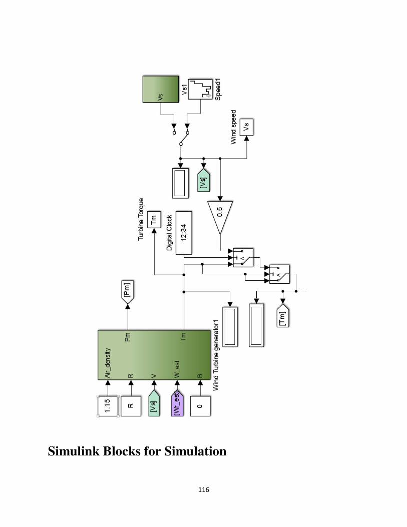
116
Simulink Blocks for Simulation

117
Ap
p.
B. 1
Ov
eral
l
WT
mo
del.
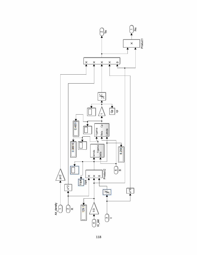
118
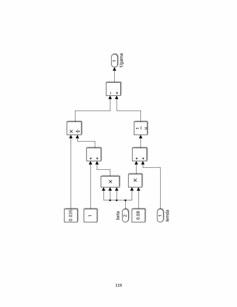
119
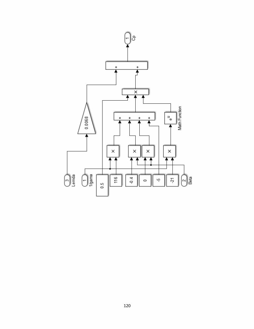
120
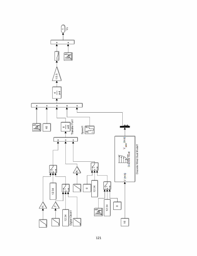
121

122
App. B. 6 Wind speed step changes.
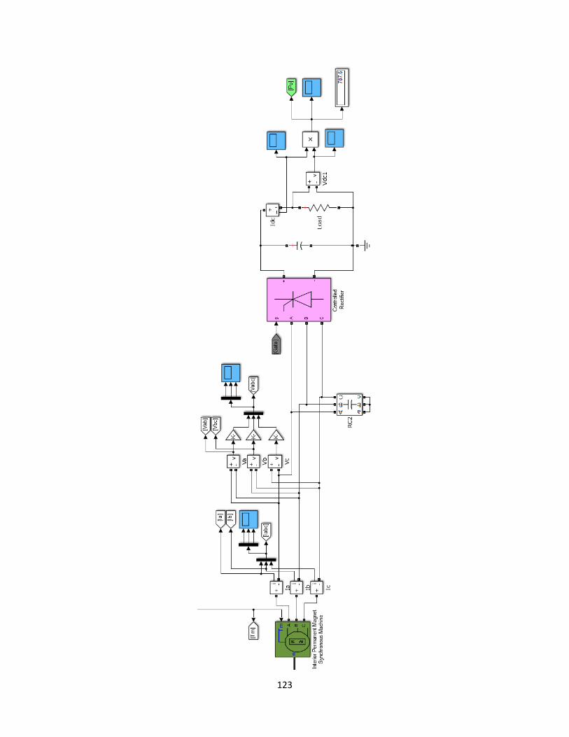
123
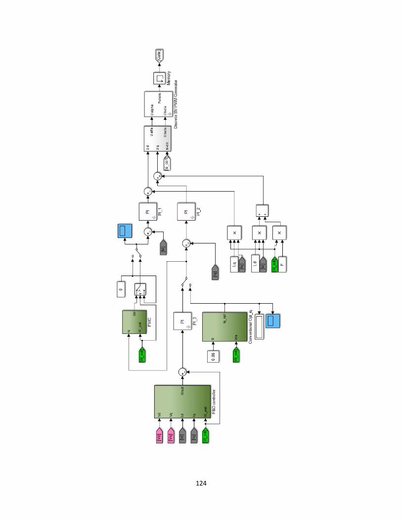
124
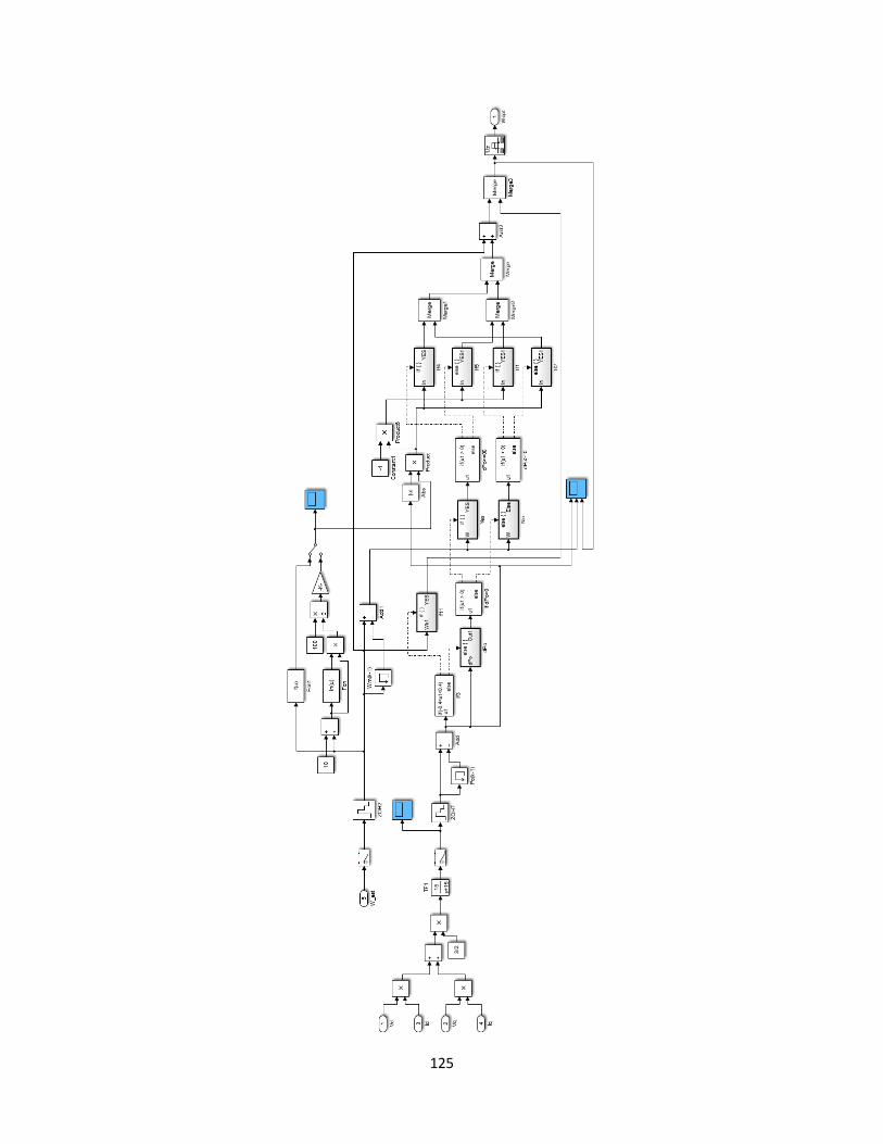
125
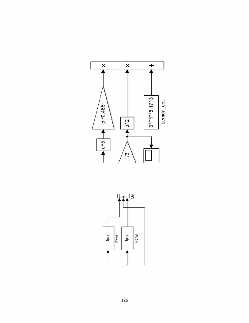
126
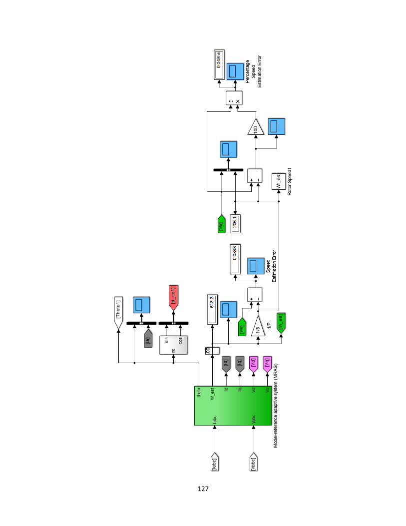
127
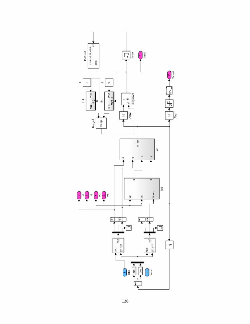
128
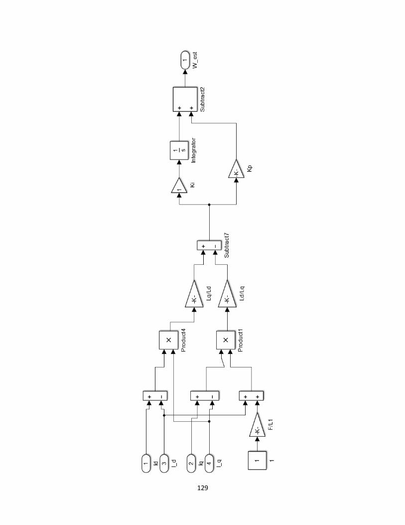
129
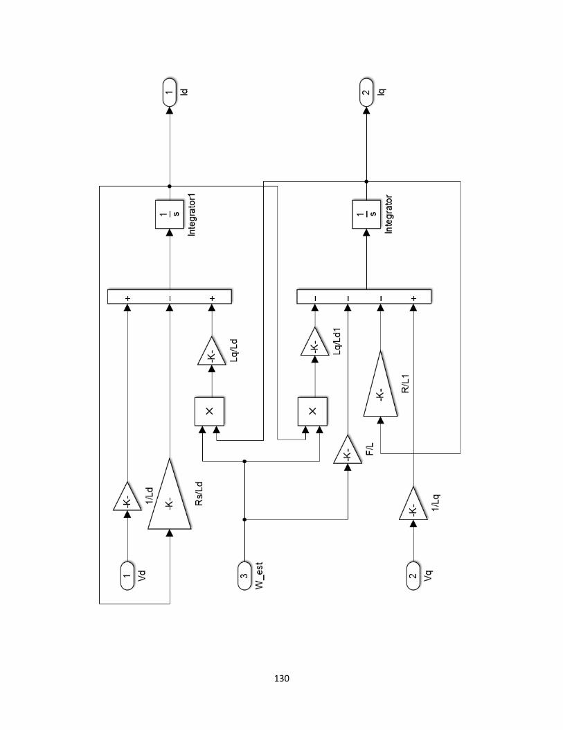
130

131
Appendix C
Drive and Interface Circuit
Base drive circuit for the inverter and interface circuit for the current sensor
R1= R2 = R3 = R4 = R5 = R6 = 1.5k
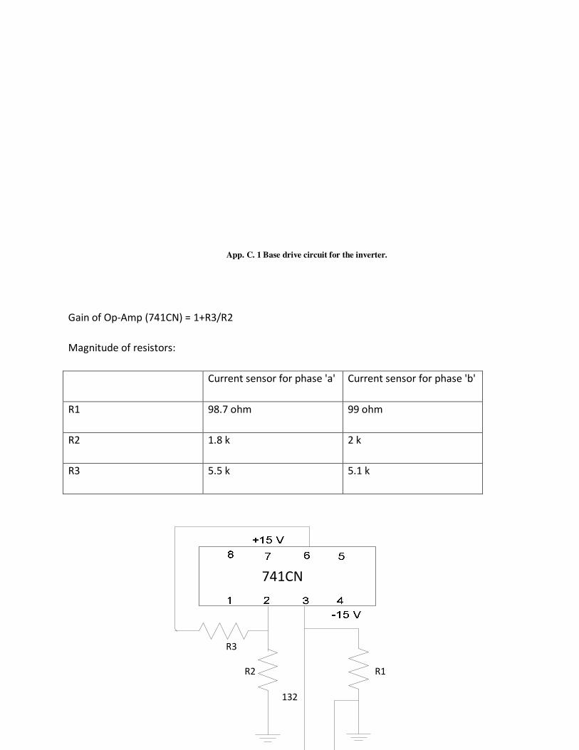
132
App. C. 1 Base drive circuit for the inverter.
Gain of Op-Amp (741CN) = 1+R3/R2
Magnitude of resistors:
Current sensor for phase 'a' Current sensor for phase 'b'
R1 98.7 ohm 99 ohm
R2 1.8 k 2 k
R3 5.5 k 5.1 k
R1 R2
R3
741CN

133
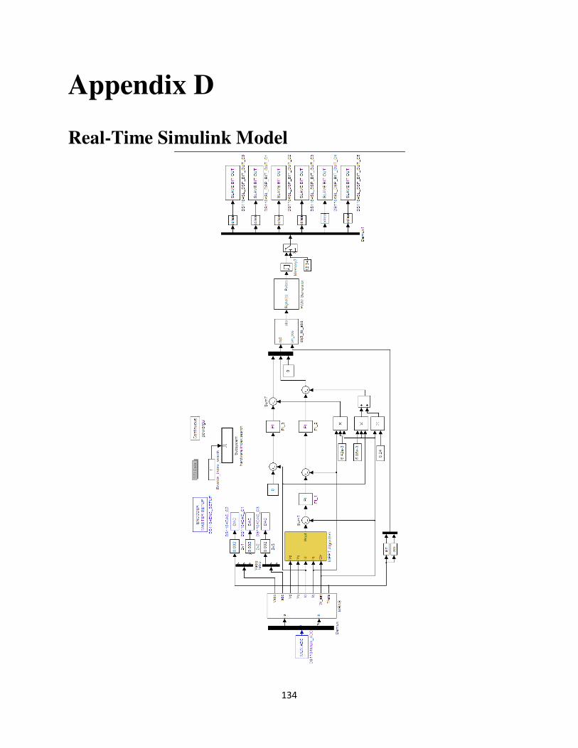
134
Appendix D
Real-Time Simulink Model
Recommended


![MRAS-based Sensorless Speed Estimation of High Speed ... 2019...Network Controller for Speed Sensorless Control of PMSM [C]. 2017 7th IEEE International Conference on Control System,](https://img.pdfslide.net/doc/110x75/6149784c080bfa626014a182/mras-based-sensorless-speed-estimation-of-high-speed-2019-network-controller.jpg)