Spike timing dependent plasticity - STDP
Markram et. al. 1997
+10 ms
-10 ms
Pre before Post: LTP
Post before Pre: LTD

Pre follows Post:Long-term Depression
Pre
tPre
Post
tPost
Synaptic
change %
Spike Timing Dependent Plasticity: Temporal Hebbian Learning
Weight-change curve (Bi&Poo, 2001)
Pre
tPre
Post
tPost
Pre precedes Post:Long-term Potentiation
Aca
usal
Causal
(possibly)
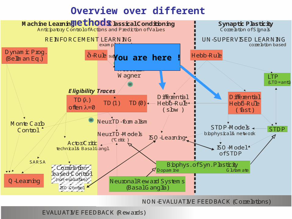
Machine Learning Classical Conditioning Synaptic Plasticity
Dynamic Prog.(Bellman Eq.)
REINFORCEMENT LEARNING UN-SUPERVISED LEARNINGexample based correlation based
d-Rule
Monte CarloControl
Q-Learning
TD( )often =0
ll
TD(1) TD(0)
Rescorla/Wagner
Neur.TD-Models(“Critic”)
Neur.TD-formalism
DifferentialHebb-Rule
(”fast”)
STDP-Modelsbiophysical & network
EVALUATIVE FEEDBACK (Rewards)
NON-EVALUATIVE FEEDBACK (Correlations)
SARSA
Correlationbased Control
(non-evaluative)
ISO-Learning
ISO-Modelof STDP
Actor/Critictechnical & Basal Gangl.
Eligibility Traces
Hebb-Rule
DifferentialHebb-Rule
(”slow”)
supervised L.
Anticipatory Control of Actions and Prediction of Values Correlation of Signals
=
=
=
Neuronal Reward Systems(Basal Ganglia)
Biophys. of Syn. PlasticityDopamine Glutamate
STDP
LTP(LTD=anti)
ISO-Control
Overview over different methods
You are here !

I. Pawlow
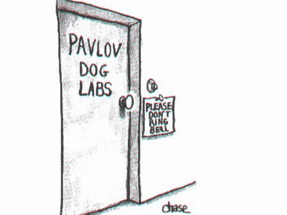
History of the Concept of TemporallyAsymmetrical Learning: Classical Conditioning

I. Pawlow
History of the Concept of TemporallyAsymmetrical Learning: Classical Conditioning
Correlating two stimuli which are shifted with respect to each other in time.
Pavlov’s Dog: “Bell comes earlier than Food”
This requires to remember the stimuli in the system.
Eligibility Trace: A synapse remains “eligible” for modification for some time after it was active (Hull 1938, then a still abstract concept).
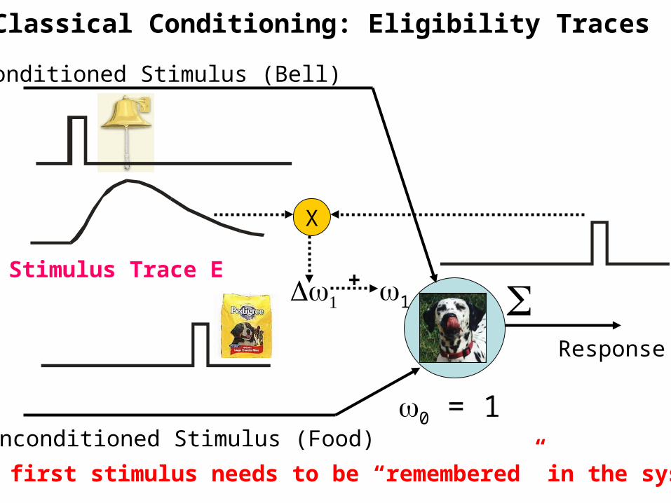
0 = 1
1
Unconditioned Stimulus (Food)
Conditioned Stimulus (Bell)
Response
X
+Stimulus Trace E
The first stimulus needs to be “remembered” in the system
Classical Conditioning: Eligibility Traces

I. Pawlow
History of the Concept of TemporallyAsymmetrical Learning: Classical Conditioning
Eligibility Traces
Note: There are vastly different time-scales for (Pavlov’s) behavioural experiments:
Typically up to 4 seconds
as compared to STDP at neurons:
Typically 40-60 milliseconds (max.)

Machine Learning Classical Conditioning Synaptic Plasticity
Dynamic Prog.(Bellman Eq.)
REINFORCEMENT LEARNING UN-SUPERVISED LEARNINGexample based correlation based
d-Rule
Monte CarloControl
Q-Learning
TD( )often =0
ll
TD(1) TD(0)
Rescorla/Wagner
Neur.TD-Models(“Critic”)
Neur.TD-formalism
DifferentialHebb-Rule
(”fast”)
STDP-Modelsbiophysical & network
EVALUATIVE FEEDBACK (Rewards)
NON-EVALUATIVE FEEDBACK (Correlations)
SARSA
Correlationbased Control
(non-evaluative)
ISO-Learning
ISO-Modelof STDP
Actor/Critictechnical & Basal Gangl.
Eligibility Traces
Hebb-Rule
DifferentialHebb-Rule
(”slow”)
supervised L.
Anticipatory Control of Actions and Prediction of Values Correlation of Signals
=
=
=
Neuronal Reward Systems(Basal Ganglia)
Biophys. of Syn. PlasticityDopamine Glutamate
STDP
LTP(LTD=anti)
ISO-Control
Overview over different methods
Mathematical formulation of learning rules is
similar but time-scales are much different.

Early: “Bell”
Late: “Food”
x
)( )( )( tytutdt
dii
Differential Hebb Learning Rule
Xi
X0
Simpler Notationx = Inputu = Traced Input
V
V’(t)
ui
u0

Defining the TraceIn general there are many ways to do this, but usually one chooses a trace that looks biologically realistic and allows for some analytical calculations, too.
EPSP-like functions:-function:
Double exp.:
This one is most easy to handle analytically and, thus, often used.
DampenedSine wave:
Shows an oscillation.
h(t) =n
0 t<0hk(t) tõ 0
h(t) = teà atk
h(t) = b1sin(bt) eà at
k
h(t) = î1(eà at à eà bt)
k
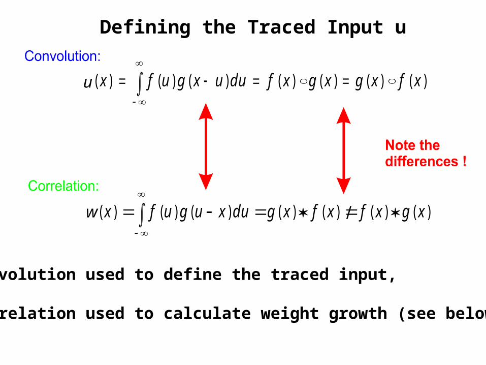
Defining the Traced Input u
Convolution used to define the traced input,
Correlation used to calculate weight growth (see below).
)()()()()()()( xfxgxgxfduuxgufxh
u
)()()()()()()( xgxfxfxgduxugufxh
w

Defining the Traced Input u
)()()()()()()( xfxgxgxfduuxgufxh
u
Specifically (we are dealing with causal functions!):
u(t) = s0
1x(ü)h(t à ü)dü
If x is a spike train(using the d-function):
Then:
For example:
u(t) =P
j=0
Mh(t à tj)
u(t) = h(t à T)
u(t) = h(t)x(t) = î (0)
x(t) = î (T)
x(t) =P
j=0
Mî (tj)

Differential Hebb Rules – The Basic Rule
General:
Two inputs only. Thuswe get for the output:
v = w0u0+ w1u1
w0=1=const.
One weight unchanging:
Same h for all inputs.
ISO rule
Isotropic Sequence Order Lng.
(as we can also allow w0 to change!)
dtdw1 = ö u1 v0
1
0
X
v
v’
ISO-Learning
h
h
x
x0
1
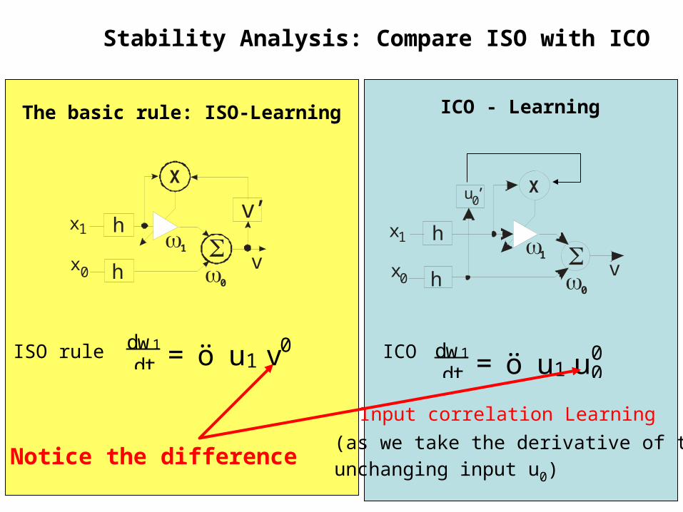
The basic rule: ISO-Learning
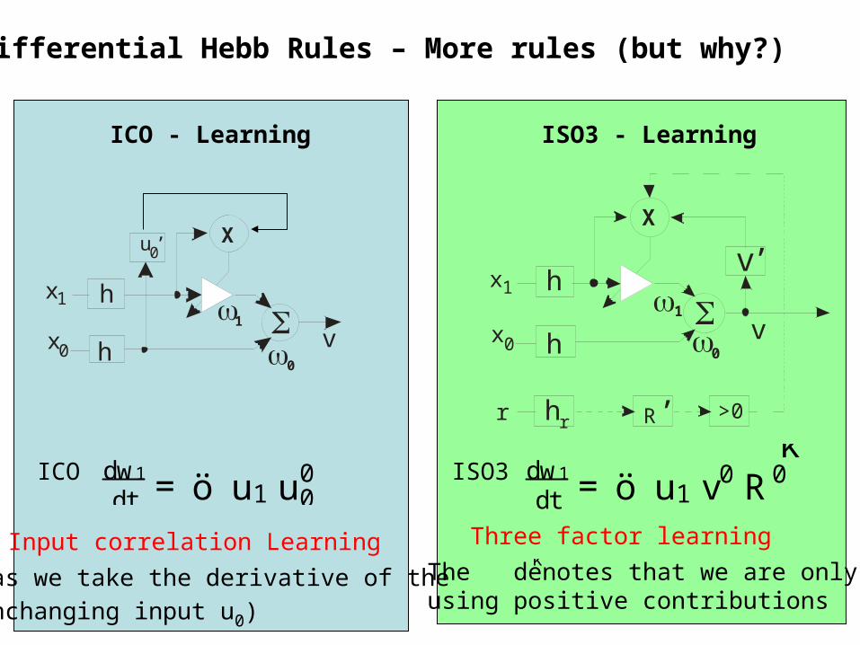
Differential Hebb Rules – More rules (but why?)
ISO3dt
dw1 = ö u1 v0 R0k
Three factor learningk
The denotes that we are onlyusing positive contributions
1
X
v
v’
ISO3-Learning
h
h
hr
x
x
r >0R’
0
1
0
ISO3 - Learning
ICO
Input correlation Learning
(as we take the derivative of the
unchanging input u0)
dtdw1 = ö u1 u0
0
1
X
v
ICO-Learning
h
h
x
x
u ’
0
0
1
0
ICO - Learning
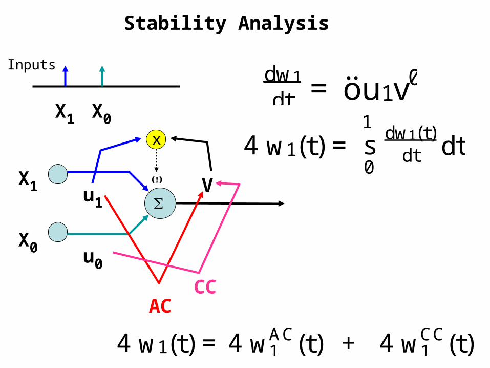
Stability Analysis
x
X1
X0
Vu1
u0
ACCC
dtdw1 = öu1v0
4 w1(t) = s0
1
dtdw1(t) dt
4 w1(t) = 4 wAC1 (t) + 4 wCC
1 (t)
X0X1
Inputs
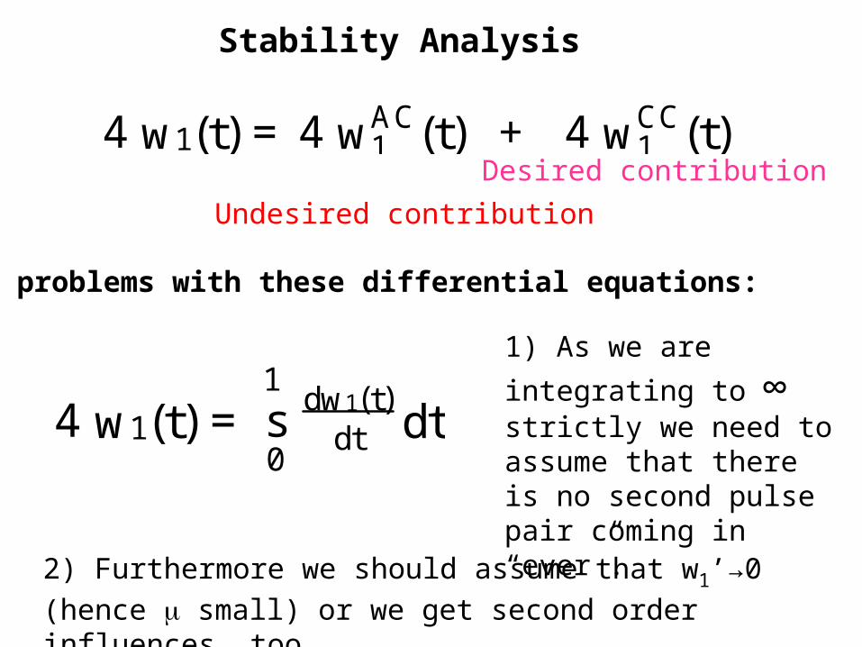
Stability Analysis
4 w1(t) = 4 wAC1 (t) + 4 wCC
1 (t)Desired contribution
Undesired contribution
Some problems with these differential equations:
4 w1(t) = s0
1
dtdw1(t) dt
1) As we are
integrating to ∞ strictly we need to assume that there is no second pulse pair coming in “ever”.
2) Furthermore we should assume that w1’→0 (hence small) or we get second order influences, too.

Stability Analysis (ISO)Under these assumptions we can calculate wAC and wCC to find out whether the rules are stable or not.
In general we assume two inputs:
x1(t) = î (t) and x0(t) = î (t à T)
dtdw1 = öu1v0and get for ISO:
4 wCC1 = w0sh(t)h0(t à T)dt = w02û
1a+baà bh(t)
4 wAC1 = w1
àesh(t)h0(tà T)dt à 1
á= w1
àe2
1h2(1 ) à 1á
= 0
ISO is (only) asymptotically stable for t→∞
X0X1
InputsT
Magn. of one step
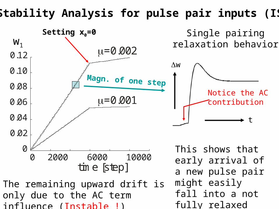
Stability Analysis for pulse pair inputs (ISO)
=0.001
=0.002
time [step]0 2000 6000 10000
0
0.02
0.04
0.06
0.08
0.10
0.12
w1
Setting x0=0
The remaining upward drift is only due to the AC term influence (Instable !)
Single pairingrelaxation behavior
This shows that early arrival of a new pulse pair might easily fall into a not fully relaxed system. (Instable !)
t
w
Notice the ACcontribution
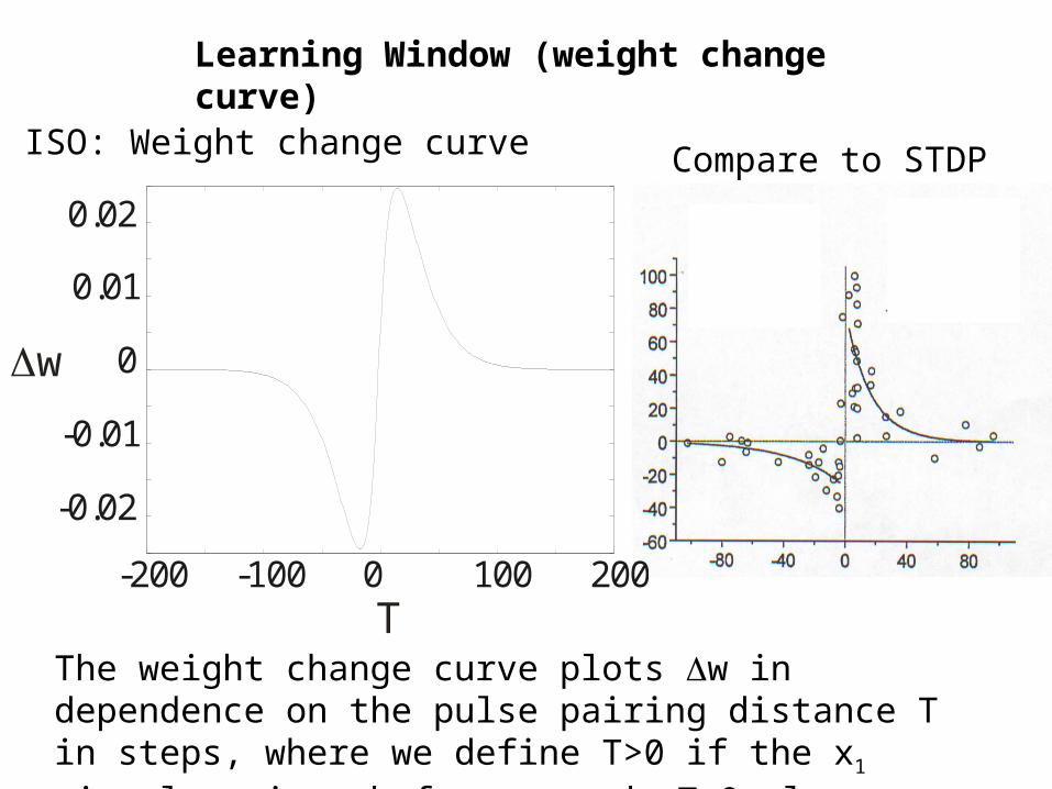
Compare to STDP
w
T-200 -100 0 100 200
-0.02
-0.01
0
0.01
0.02
ISO: Weight change curve
Learning Window (weight change curve)
The weight change curve plots w in dependence on the pulse pairing distance T in steps, where we define T>0 if the x1 signal arrives before x0 and T<0 else.
ISO ruledt
dw1 = ö u1 v0
1
0
X
v
v’
ISO-Learning
h
h
x
x0
1
The basic rule: ISO-Learning
ICO
Input correlation Learning
(as we take the derivative of the
unchanging input u0)
dtdw1 = ö u1 u0
0
1
X
v
ICO-Learning
h
h
x
x
u ’
0
0
1
0
ICO - Learning
Stability Analysis: Compare ISO with ICO
Notice the difference
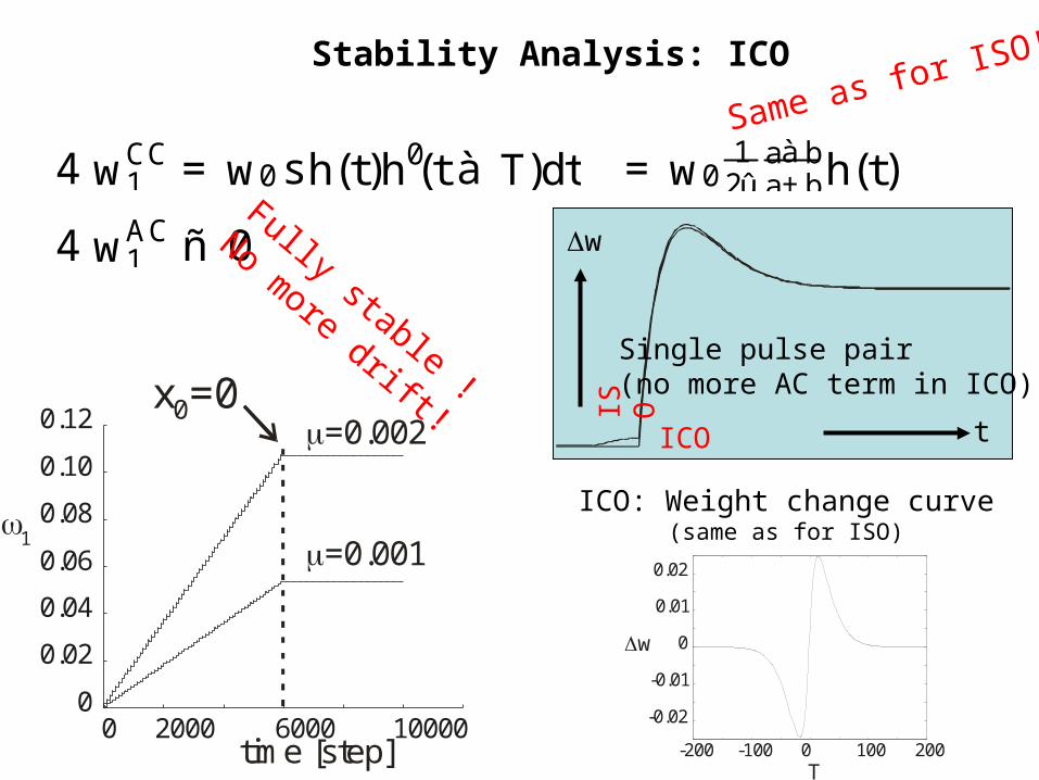
Stability Analysis: ICO
4 wAC1 ñ 0
4 wCC1 = w0sh(t)h0(t à T)dt = w02û
1a+baà bh(t)Same as for ISO!
Fully stable !
No more drift!
=0.001
=0.002
time [step]
1
0 2000 6000 100000
0.02
0.04
0.06
0.08
0.10
0.12x =00
w
T-200 -100 0 100 200
-0.02
-0.01
0
0.01
0.02
ICO: Weight change curve(same as for ISO)
Single pulse pair(no more AC term in ICO).
IS O
ICO t
w

ISO ruledt
dw1 = ö u1 v0
1
0
X
v
v’
ISO-Learning
h
h
x
x0
1
The basic rule: ISO-Learning
ICOdt
dw1 = ö u1 u00
1
X
v
ICO-Learning
h
h
x
x
u ’
0
0
1
0
ICO - Learning
Stability Analysis: More comparisons
Conjoint learning-control-signal (same for all inputs !)
Single input as designated learning-control-signal.
Makes ICO a heterosynaptic rule of questionable biological realism.

Stability Analysis: More comparisonsThis difference is especially visible when wanting to symmetrize the rules (both weights can change!).
X
X
v
v’h
h
x
x0
1i
ISO-Sym One control signal !
T=18
1
0
-3.5-3
-2.5-2
-1.5-1
-0.5 0
0.5 1
1.5 2
0 2 4 6 8 10time [steps]
x106
X
X
v
h
h
x
x0
1 1
0
d/dt
ICO-SymTwocontrolsignals !
time [steps]
-0.2
-0.1
0
0.1
0.2
0 2000 4000 6000 8000 10000
T=15

time [steps]
-0.2
-0.1
0
0.1
0.2
0 2000 4000 6000 8000 10000
T=15
ICO-sym is truly symmetrical, but needs two control signals.
ISO-sym behaves in a difficult and unstable oscillatory way.
X0X1
InputsT
Synapse w1 grows because x1 is before x0.
The Effects of Symmetry
Synapse w0 shrinks because x0 is after x1.

ISO3: uses – like ISO – a single learning-control-signal
ISO3dt
dw1 = ö u1 v0 R0k
1
X
v
v’
ISO3-Learning
h
h
hr
x
x
r >0R’
0
1
0
ISO3 - LearningIdea: The system should learn ONLY at that moment in time when there was a “relevant” event r !
We use a shorter trace for r, as it should remain rather restricted in time.
Same filter function h but parameters ar and br.
We also define Tr as the
interval between x1 and r. Many times Tr=T, hence r occurs together with x0.
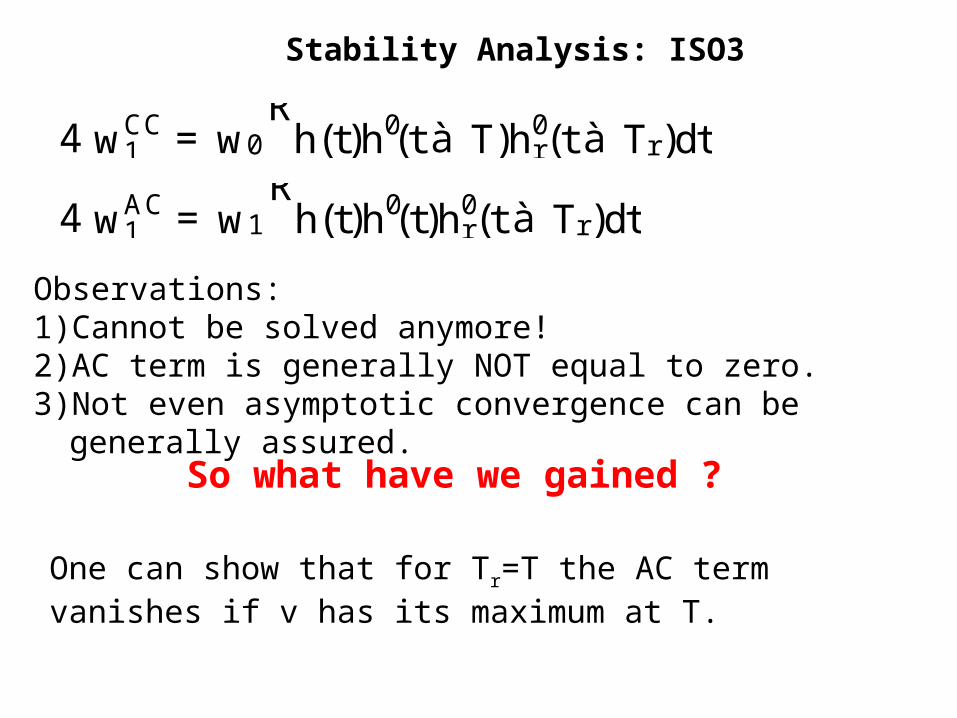
Stability Analysis: ISO3
4 wAC1 = w1
Rh(t)h0(t)h0
r(t à Tr)dt
4 wCC1 = w0
Rh(t)h0(t à T)h0
r(t à Tr)dt
Observations:1) Cannot be solved anymore!2) AC term is generally NOT equal to zero.3) Not even asymptotic convergence can be generally assured.
So what have we gained ?
One can show that for Tr=T the AC term vanishes if v has its maximum at T.

u1'
Stability Analysis: ISO3, graphical proof
x0x1
u0
r
Maximum at T
T
AC
CCContributions of AC and CCgraphically depicted
u1
v0(t) = u01(t); t < T
as x0 has not yet happened
limt! Tà
v0(t) = 0
If we restrict learning to the moment when x0 occurs then we do not have any AC contribution.
!! A questionable assumption: argmax(u1) = T !!
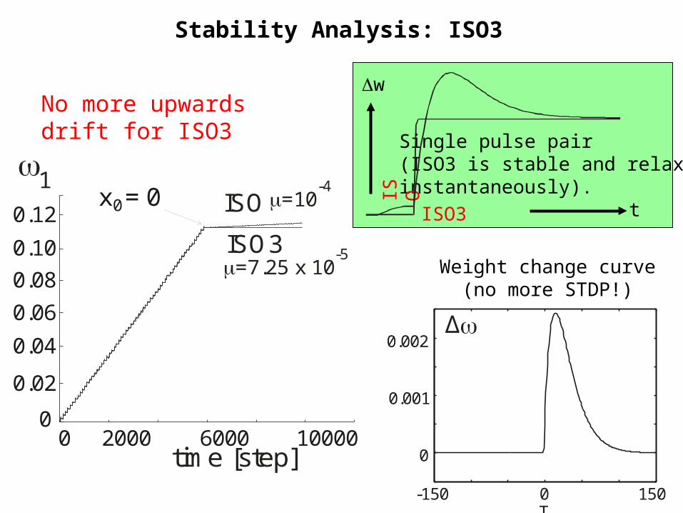
Stability Analysis: ISO3
=7.25 x 10-5
=10-4
time [step]0 2000 6000 10000
0x = 01
0
0.02
0.04
0.06
0.08
0.10
0.12 ISO
ISO3
Single pulse pair(ISO3 is stable and relaxesinstantaneously).IS O
ISO3 t
w
∆
-150 0T
150
0
0.001
0.002
Weight change curve(no more STDP!)
No more upwards drift for ISO3

A General Problem: T is usually unknown and variable
Introducing a filter bank: (example ISO)
0
1
11
N
1
N
X
X
xu
u
xu
00
11
1
v
v’
1
1
1
N
0
h
h
h
N1 uu 11
Spreading out the earlier input over time!
Remember: “A questionable assumption: argmax(u1) = T”
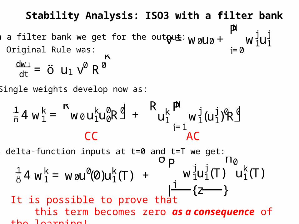
Stability Analysis: ISO3 with a filter bank
With a filter bank we get for the output: v = w0u0+P
j=0
Nwj
1uj1
ö14 wk
1 =R
w0uk1u
00R
0 +
Single weights develop now as:
Ruk
1
P
j=1
Nwj
1(uj1)
0R0
dtdw1 = ö u1 v0 R0
kOriginal Rule was:
CC ACWith delta-function inputs at t=0 and t=T we get:
ö14 wk
1 = w0u0(0)uk1(T) +
ð P
jwj
1uj1(T)
ñ0uk
1(T)
It is possible to prove that this term becomes zero as a consequence of the learning!
| {z }
Recommended