1
Stability of End Notched Flexure Specimen
Master’s (one year) Degree Thesis in Applied Mechanics Level 30 ECTS Spring term, 2010 Arun Gojuri Supervisor: Ulf Stigh Examiner: Thomas Carlberger
School of Technology & Society Skövde University
BOX 408 SE-541 28 Skövde
Sweden
MA
STE
R’S
DE
GR
EE
TH
ESI
S

2
Preface
This work has been carried out during the spring semester year 2010 at the Department of
Mechanical Engineering at the University of Skövde, Sweden.
First and foremost, I would like say thanks to my supervisor Prof. Ulf Stigh not only for
his help and support, but also for sharing the knowledge and for always being able to help.
Moreover, for the opportunity to perform this thesis work and also for his way of making
the topic exciting and interesting.
In a deep thanks to Dr. Kent Salomonsson, Dr. Tobias Andersson and Dr. Anders Biel for
their great supports during my theoretical lectures works and commitment concerning
various software related issues.
Also thanks to my friends Tomas Walander, Daniel Svensson, and Saidul Gundeboina for
help and sharing knowledge with me during this work.
Finally yet importantly, wide thanks are dedicated to the examiner, Dr. Thomas Carlberger
for giving an opportunity to present my thesis work here.
Skövde. December 2010
Arun Gojuri
3
Abstract
This paper deals with two-dimensional Finite Element Analysis of the End Notched
Flexure (ENF) specimen. The specimen is known to be unstable if the crack length is
shorter than some critical crack length acr. A geometric linear two-dimensional Finite
Element (FE) analysis of the ENF specimen is performed to evaluate acr for isotropic and
orthotropic elastic materials, respectively. Moreover, the Mode II Energy Release Rate
(ERR) JII and the compliance of the specimen are calculated. The influence of anisotropy
is studied. Comparisons are made with the results from beam theory. This work is an
extension of previous work.
Keywords: Energy release rate, Finite element method, ENF-specimen, Delamination,
Composite materials isotropic & orthotropic, Controlled displacement.
4
Table of Contents
Preface ................................................................................................................. 2
Abstract ............................................................................................................... 3
1. Introduction ................................................................................................. 5
1.1 ENF specimen .......................................................................................................................... 5
1.2 Contour integral J .................................................................................................................... 7
1.3 Isotropic material .................................................................................................................. 8
1.4 Orthotropic material ............................................................................................................ 9
2. Materials and method ............................................................................. 10
2.1 Geometry of specimen ..................................................................................................... 10
2.2 Material properties ............................................................................................................ 10
2.3 Finite element method simulations ............................................................................ 11
2.4 Evaluation of J ....................................................................................................................... 12
3. Numerical studies ................................................................................... 13
4. Discussion and Conclusion .................................................................. 16
5. References .................................................................................................. 17
5
1. Introduction
Much work has recently been devoted to the failure mechanism of composites.
Consequently, many new fracture tests have been devised for measuring the fracture
properties. Most such tests and standard test procedures are limited to studies of
delamination where a crack propagates between the plies. Fracture mechanics are
commonly employed to accommodate crack tip singularities, and the energy release rate
(ERR) is a physically well-defined quantity that is experimentally measurable using the
compliance technique (Russell & Street, 1982 and Broek, 1984).
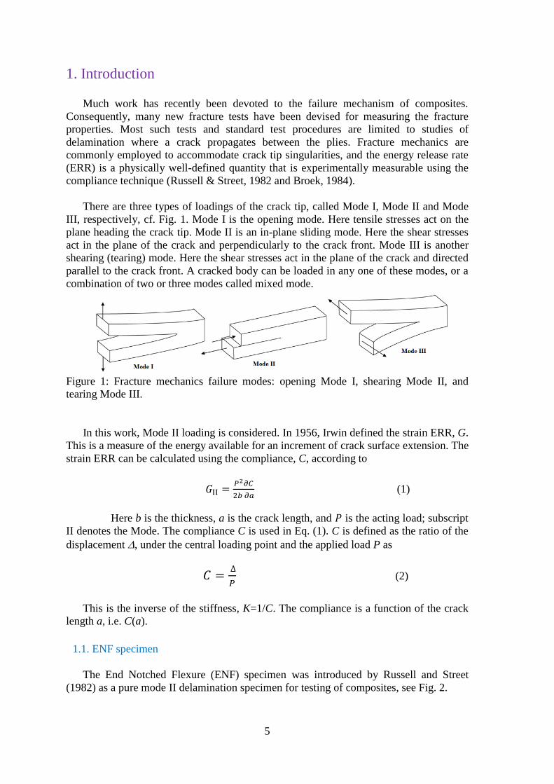
There are three types of loadings of the crack tip, called Mode I, Mode II and Mode
III, respectively, cf. Fig. 1. Mode I is the opening mode. Here tensile stresses act on the
plane heading the crack tip. Mode II is an in-plane sliding mode. Here the shear stresses
act in the plane of the crack and perpendicularly to the crack front. Mode III is another
shearing (tearing) mode. Here the shear stresses act in the plane of the crack and directed
parallel to the crack front. A cracked body can be loaded in any one of these modes, or a
combination of two or three modes called mixed mode.
Figure 1: Fracture mechanics failure modes: opening Mode I, shearing Mode II, and
tearing Mode III.
In this work, Mode II loading is considered. In 1956, Irwin defined the strain ERR, G.
This is a measure of the energy available for an increment of crack surface extension. The
strain ERR can be calculated using the compliance, C, according to
(1)
Here b is the thickness, a is the crack length, and is the acting load; subscript
II denotes the Mode. The compliance C is used in Eq. (1). C is defined as the ratio of the
displacement , under the central loading point and the applied load P as
(2)
This is the inverse of the stiffness, K=1/C. The compliance is a function of the crack
length a, i.e. C(a).
1.1. ENF specimen
The End Notched Flexure (ENF) specimen was introduced by Russell and Street
(1982) as a pure mode II delamination specimen for testing of composites, see Fig. 2.
6
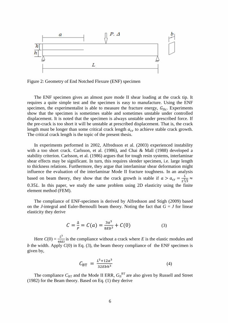
Figure 2: Geometry of End Notched Flexure (ENF) specimen
The ENF specimen gives an almost pure mode II shear loading at the crack tip. It
requires a quite simple test and the specimen is easy to manufacture. Using the ENF
specimen, the experimentalist is able to measure the fracture energy, . Experiments
show that the specimen is sometimes stable and sometimes unstable under controlled
displacement. It is noted that the specimen is always unstable under prescribed force. If
the pre-crack is too short it will be unstable at prescribed displacement. That is, the crack
length must be longer than some critical crack length to achieve stable crack growth.
The critical crack length is the topic of the present thesis.
In experiments performed in 2002, Alfredsson et al. (2003) experienced instability
with a too short crack. Carlsson, et al. (1986), and Chai & Mall (1988) developed a
stability criterion. Carlsson, et al. (1986) argues that for tough resin systems, interlaminar
shear effects may be significant. In turn, this requires slender specimen, i.e. large length
to thickness relations. Furthermore, they argue that interlaminar shear deformation might
influence the evaluation of the interlaminar Mode II fracture toughness. In an analysis
based on beam theory, they show that the crack growth is stable if
. In this paper, we study the same problem using 2D elasticity using the finite
element method (FEM).
The compliance of ENF-specimen is derived by Alfredsson and Stigh (2009) based
on the J-integral and Euler-Bernoulli beam theory. Noting the fact that G = J for linear
elasticity they derive
(3)
Here C(0) =
is the compliance without a crack where E is the elastic modules and
b the width. Apply C(0) in Eq. (3), the beam theory compliance of the ENF specimen is
given by,
(4)
The compliance CBT and the Mode II ERR, GIIBT
are also given by Russell and Street
(1982) for the Beam theory. Based on Eq. (1) they derive
7
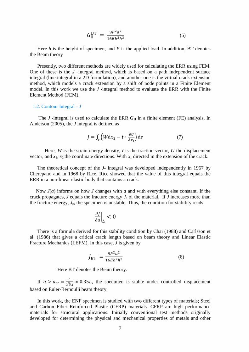
(5)
Here h is the height of specimen, and P is the applied load. In addition, BT denotes
the Beam theory
Presently, two different methods are widely used for calculating the ERR using FEM.
One of these is the J -integral method, which is based on a path independent surface
integral (line integral in a 2D formulation), and another one is the virtual crack extension
method, which models a crack extension by a shift of node points in a Finite Element
model. In this work we use the J -integral method to evaluate the ERR with the Finite
Element Method (FEM).
1.2. Contour Integral - J
The J -integral is used to calculate the ERR GII in a finite element (FE) analysis. In
Anderson (2005), the J integral is defined as
(7)
Here, W is the strain energy density, t is the traction vector, U the displacement
vector, and x1, x2 the coordinate directions. With x1 directed in the extension of the crack.
The theoretical concept of the J- integral was developed independently in 1967 by
Cherepano and in 1968 by Rice. Rice showed that the value of this integral equals the
ERR in a non-linear elastic body that contains a crack.
Now J(a) informs on how J changes with a and with everything else constant. If the
crack propagates, J equals the fracture energy Jc of the material. If J increases more than
the fracture energy, Jc, the specimen is unstable. Thus, the condition for stability reads
There is a formula derived for this stability condition by Chai (1988) and Carlsson et
al. (1986) that gives a critical crack length based on beam theory and Linear Elastic
Fracture Mechanics (LEFM). In this case, J is given by
(8)
Here BT denotes the Beam theory.
If
, the specimen is stable under controlled displacement
based on Euler-Bernoulli beam theory.
In this work, the ENF specimen is studied with two different types of materials; Steel
and Carbon Fiber Reinforced Plastic (CFRP) materials. CFRP are high performance
materials for structural applications. Initially conventional test methods originally
developed for determining the physical and mechanical properties of metals and other
8
homogeneous and isotropic engineering materials were used with CFRP. It was soon
recognized that these new anisotropic (orthotropic) materials require special
consideration for determining their physical and mechanical properties.
Carbon fiber reinforced polymer is a polymer matrix composite material reinforced
by carbon fibers. Carbon fibers are very expensive and are used for reinforcing polymer
matrix due to the following properties. They have very high specific modulus of
elasticity, exceeding that of steel, high tensile strength, and low density, Daniel and Ishai
(1994).
1.3. Isotropic material
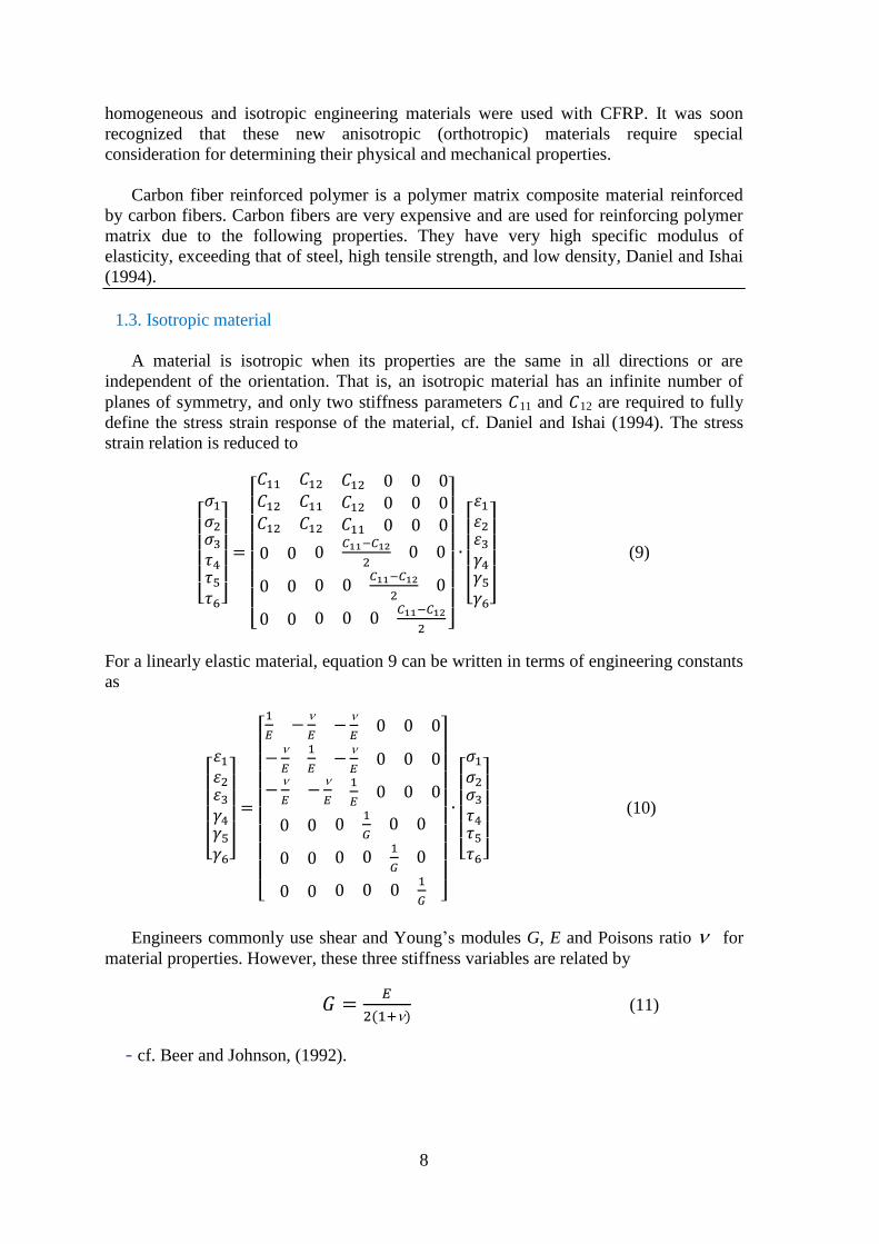
A material is isotropic when its properties are the same in all directions or are
independent of the orientation. That is, an isotropic material has an infinite number of
planes of symmetry, and only two stiffness parameters 11 and 12 are required to fully
define the stress strain response of the material, cf. Daniel and Ishai (1994). The stress
strain relation is reduced to
(9)
For a linearly elastic material, equation 9 can be written in terms of engineering constants
as
(10)
Engineers commonly use shear and Young’s modules G, E and Poisons ratio for
material properties. However, these three stiffness variables are related by
(11)
- cf. Beer and Johnson, (1992).
9
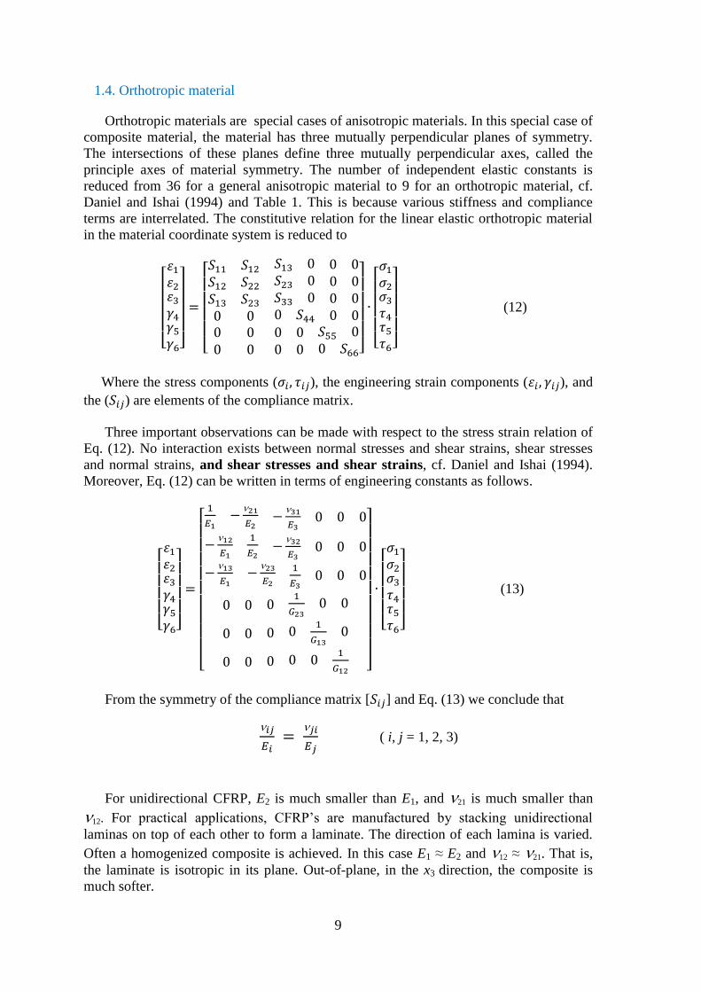
1.4. Orthotropic material
Orthotropic materials are special cases of anisotropic materials. In this special case of
composite material, the material has three mutually perpendicular planes of symmetry.
The intersections of these planes define three mutually perpendicular axes, called the
principle axes of material symmetry. The number of independent elastic constants is
reduced from 36 for a general anisotropic material to 9 for an orthotropic material, cf.
Daniel and Ishai (1994) and Table 1. This is because various stiffness and compliance
terms are interrelated. The constitutive relation for the linear elastic orthotropic material
in the material coordinate system is reduced to
(12)
Where the stress components ( ), the engineering strain components ( ), and
the ( ) are elements of the compliance matrix.
Three important observations can be made with respect to the stress strain relation of
Eq. (12). No interaction exists between normal stresses and shear strains, shear stresses
and normal strains, and shear stresses and shear strains, cf. Daniel and Ishai (1994).
Moreover, Eq. (12) can be written in terms of engineering constants as follows.
(13)
From the symmetry of the compliance matrix [ ] and Eq. (13) we conclude that
( i, j = 1, 2, 3)
For unidirectional CFRP, E2 is much smaller than E1, and 21 is much smaller than
12. For practical applications, CFRP’s are manufactured by stacking unidirectional
laminas on top of each other to form a laminate. The direction of each lamina is varied.
Often a homogenized composite is achieved. In this case E1 ≈ E2 and 12 ≈ 21. That is,
the laminate is isotropic in its plane. Out-of-plane, in the x3 direction, the composite is
much softer.
10
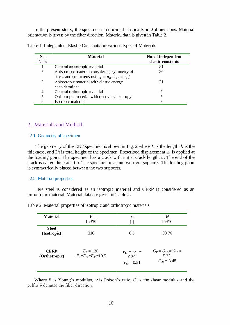
In the present study, the specimen is deformed elastically in 2 dimensions. Material
orientation is given by the fiber direction. Material data is given in Table 2.
Table 1: Independent Elastic Constants for various types of Materials
Sl.
No’s Material No. of independent
elastic constants
1 General anisotropic material 81
2 Anisotropic material considering symmetry of
stress and strain tensors( ) 36
3 Anisotropic material with elastic energy
considerations
21
4 General orthotropic material 9
5
6
Orthotropic material with transverse isotropy
Isotropic material
5
2
2. Materials and Method
2.1. Geometry of specimen
The geometry of the ENF specimen is shown in Fig. 2 where L is the length, b is the
thickness, and 2h is total height of the specimen. Prescribed displacement , is applied at
the loading point. The specimen has a crack with initial crack length, a. The end of the
crack is called the crack tip. The specimen rests on two rigid supports. The loading point
is symmetrically placed between the two supports.
2.2. Material properties
Here steel is considered as an isotropic material and CFRP is considered as an
orthotropic material. Material data are given in Table 2.
Table 2: Material properties of isotropic and orthotropic materials
Material E
[GPa] [-]
G
[GPa]
Steel
(Isotropic)
210
0.3
80.76
CFRP
(Orthotropic)
EF = 120,
ET=E22=E33=10.5 12 = 13 =
0.30
23 = 0.51
GT = G12 = G13 =
5.25,
G23 = 3.48
Where E is Young’s modulus, is Poison’s ratio, G is the shear modulus and the
suffix F denotes the fiber direction.
11
2.3. Finite Element Method simulations
In the present study, FE simulation of the ENF specimen is performed using
ABAQUS solver version 6.92 to evaluate the ERR using the J -integral. The results
obtained from FEM are compared with results from Beam theory.
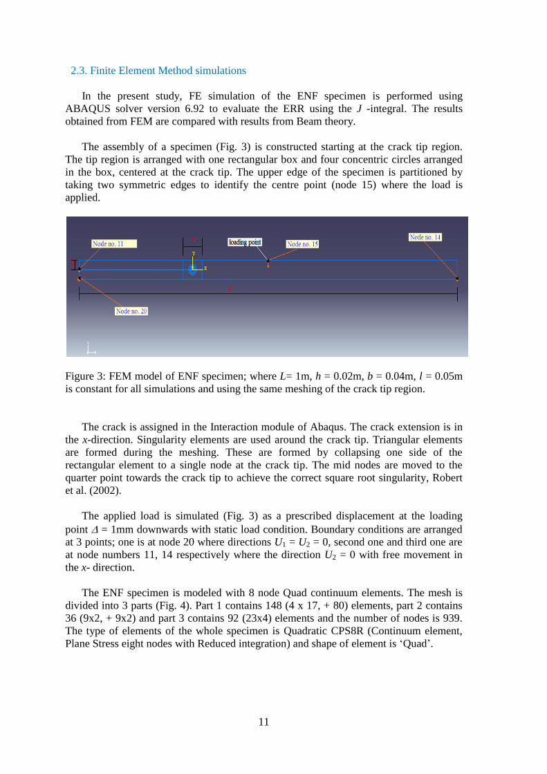
The assembly of a specimen (Fig. 3) is constructed starting at the crack tip region.
The tip region is arranged with one rectangular box and four concentric circles arranged
in the box, centered at the crack tip. The upper edge of the specimen is partitioned by
taking two symmetric edges to identify the centre point (node 15) where the load is
applied.
Figure 3: FEM model of ENF specimen; where L= 1m, h = 0.02m, b = 0.04m, l = 0.05m
is constant for all simulations and using the same meshing of the crack tip region.
The crack is assigned in the Interaction module of Abaqus. The crack extension is in
the x-direction. Singularity elements are used around the crack tip. Triangular elements
are formed during the meshing. These are formed by collapsing one side of the
rectangular element to a single node at the crack tip. The mid nodes are moved to the
quarter point towards the crack tip to achieve the correct square root singularity, Robert
et al. (2002).
The applied load is simulated (Fig. 3) as a prescribed displacement at the loading
point = 1mm downwards with static load condition. Boundary conditions are arranged
at 3 points; one is at node 20 where directions U1 = U2 = 0, second one and third one are
at node numbers 11, 14 respectively where the direction U2 = 0 with free movement in
the x- direction.
The ENF specimen is modeled with 8 node Quad continuum elements. The mesh is
divided into 3 parts (Fig. 4). Part 1 contains 148 (4 x 17, + 80) elements, part 2 contains
36 (9x2, + 9x2) and part 3 contains 92 (23x4) elements and the number of nodes is 939.
The type of elements of the whole specimen is Quadratic CPS8R (Continuum element,
Plane Stress eight nodes with Reduced integration) and shape of element is ‘Quad’.
12
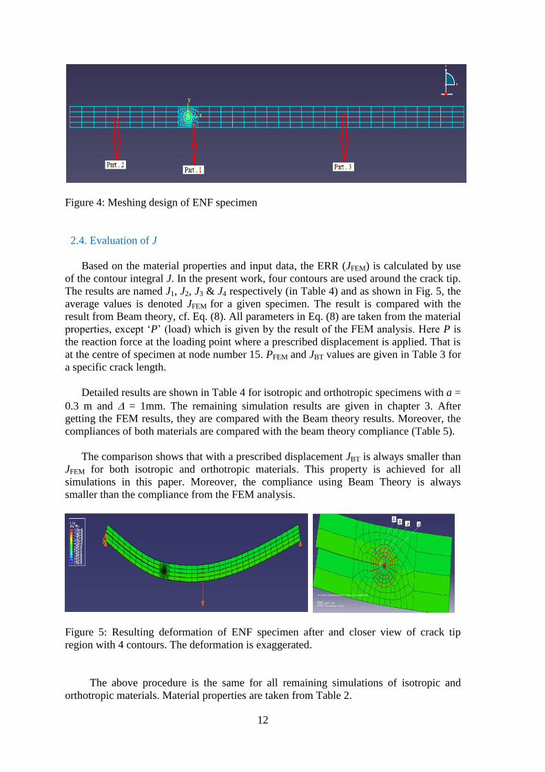
Figure 4: Meshing design of ENF specimen
2.4. Evaluation of J
Based on the material properties and input data, the ERR (JFEM) is calculated by use
of the contour integral J. In the present work, four contours are used around the crack tip.
The results are named J1, J2, J3 & J4 respectively (in Table 4) and as shown in Fig. 5, the
average values is denoted JFEM for a given specimen. The result is compared with the
result from Beam theory, cf. Eq. (8). All parameters in Eq. (8) are taken from the material
properties, except ‘P’ (load) which is given by the result of the FEM analysis. Here P is
the reaction force at the loading point where a prescribed displacement is applied. That is
at the centre of specimen at node number 15. PFEM and JBT values are given in Table 3 for
a specific crack length.
Detailed results are shown in Table 4 for isotropic and orthotropic specimens with a =
0.3 m and = 1mm. The remaining simulation results are given in chapter 3. After
getting the FEM results, they are compared with the Beam theory results. Moreover, the
compliances of both materials are compared with the beam theory compliance (Table 5).
The comparison shows that with a prescribed displacement JBT is always smaller than
JFEM for both isotropic and orthotropic materials. This property is achieved for all
simulations in this paper. Moreover, the compliance using Beam Theory is always
smaller than the compliance from the FEM analysis.
Figure 5: Resulting deformation of ENF specimen after and closer view of crack tip
region with 4 contours. The deformation is exaggerated.
The above procedure is the same for all remaining simulations of isotropic and
orthotropic materials. Material properties are taken from Table 2.
13
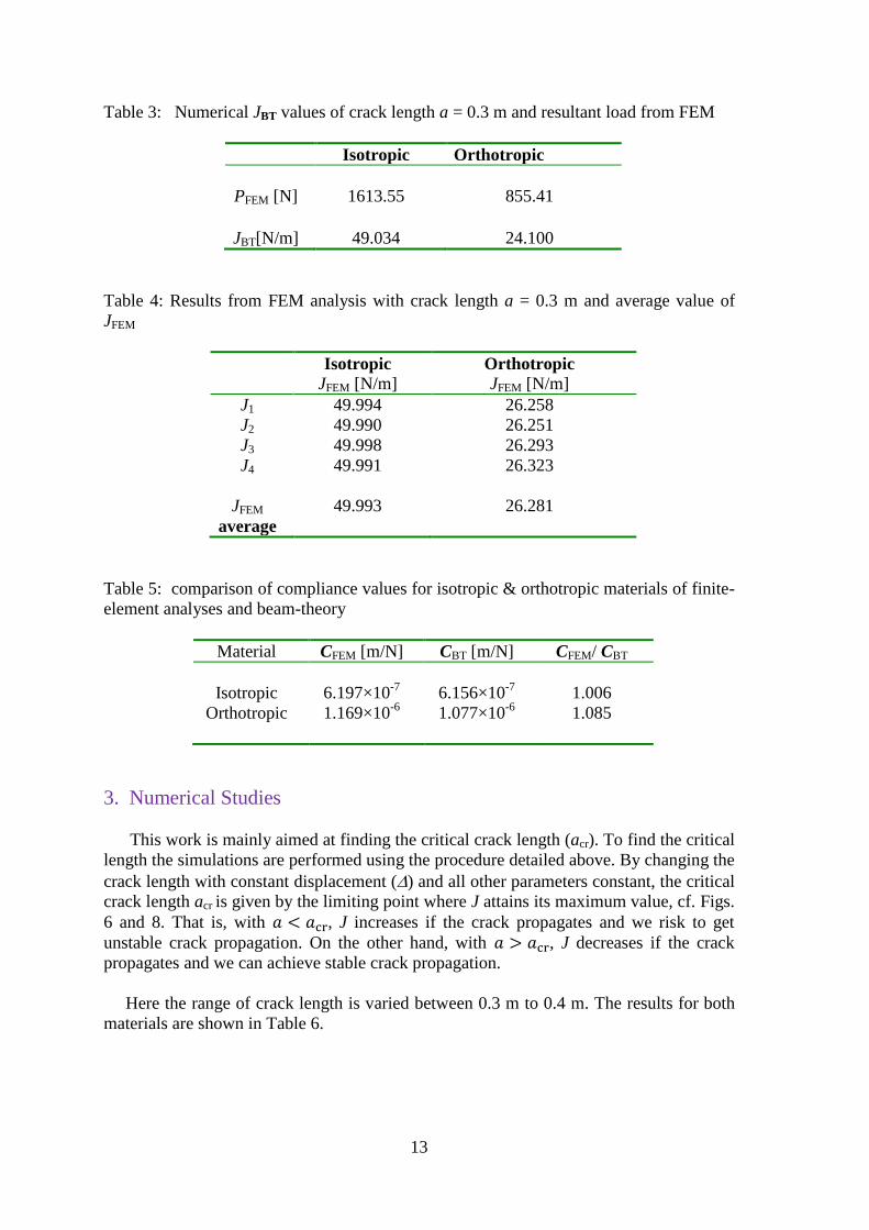
Table 3: Numerical JBT values of crack length a = 0.3 m and resultant load from FEM
Isotropic Orthotropic
PFEM [N] 1613.55 855.41
JBT[N/m]
49.034
24.100
Table 4: Results from FEM analysis with crack length a = 0.3 m and average value of
JFEM
Isotropic
JFEM [N/m] Orthotropic
JFEM [N/m]
J1 49.994 26.258
J2 49.990 26.251
J3 49.998 26.293
J4 49.991 26.323
JFEM
average
49.993
26.281
Table 5: comparison of compliance values for isotropic & orthotropic materials of finite-
element analyses and beam-theory
Material CFEM [m/N] CBT [m/N] CFEM/ CBT
Isotropic
Orthotropic
6.197×10⁻⁷
1.169×10⁻⁶
6.156×10⁻⁷
1.077×10⁻⁶
1.006
1.085
3. Numerical Studies
This work is mainly aimed at finding the critical crack length (acr). To find the critical
length the simulations are performed using the procedure detailed above. By changing the
crack length with constant displacement () and all other parameters constant, the critical
crack length acr is given by the limiting point where J attains its maximum value, cf. Figs.
6 and 8. That is, with , J increases if the crack propagates and we risk to get
unstable crack propagation. On the other hand, with , J decreases if the crack
propagates and we can achieve stable crack propagation.
Here the range of crack length is varied between 0.3 m to 0.4 m. The results for both
materials are shown in Table 6.
14
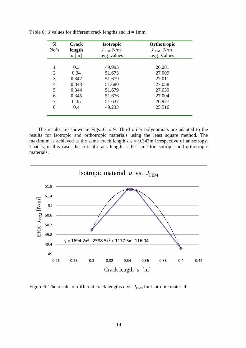
Table 6: J values for different crack lengths and = 1mm.
Sl
No’s Crack
length
a [m]
Isotropic
JFEM[N/m]
avg. values
Orthotropic
JFEM [N/m]
avg. Values
1
2
3
4
5
6
7
8
0.3
0.34
0.342
0.343
0.344
0.345
0.35
0.4
49.993
51.673
51.679
51.680
51.679
51.676
51.637
49.233
26.281
27.009
27.011
27.058
27.039
27.004
26.977
25.516
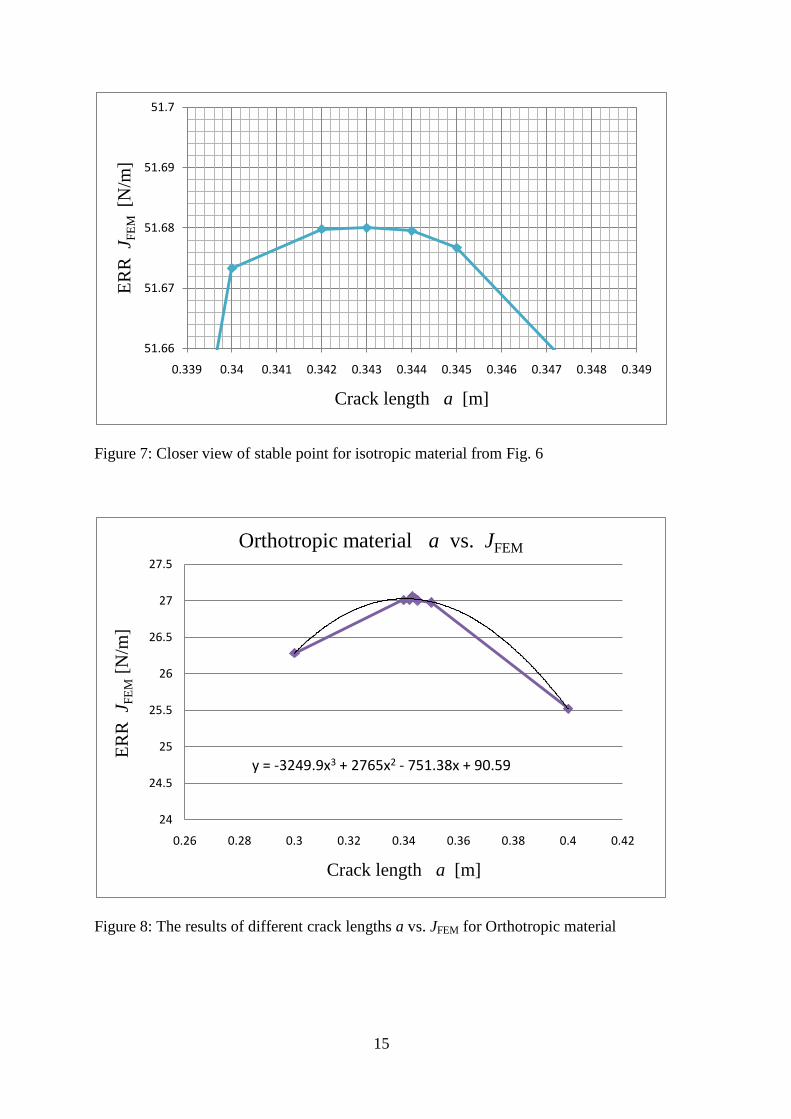
The results are shown in Figs. 6 to 9. Third order polynomials are adapted to the
results for isotropic and orthotropic materials using the least square method. The
maximum is achieved at the same crack length acr = 0.343m irrespective of anisotropy.
That is, in this case, the critical crack length is the same for isotropic and orthotropic
materials.
Figure 6: The results of different crack lengths a vs. JFEM for Isotropic material.
y = 1694.2x3 - 2588.5x2 + 1177.5x - 116.04
49
49.4
49.8
50.2
50.6
51
51.4
51.8
0.26 0.28 0.3 0.32 0.34 0.36 0.38 0.4 0.42
ER
R
J FE
M[N
/m]
Crack length a [m]
Isotropic material a vs. JFEM
15
Figure 7: Closer view of stable point for isotropic material from Fig. 6
Figure 8: The results of different crack lengths a vs. JFEM for Orthotropic material
51.66
51.67
51.68
51.69
51.7
0.339 0.34 0.341 0.342 0.343 0.344 0.345 0.346 0.347 0.348 0.349
ER
R J F
EM
[N
/m]
Crack length a [m]
y = -3249.9x3 + 2765x2 - 751.38x + 90.59
24
24.5
25
25.5
26
26.5
27
27.5
0.26 0.28 0.3 0.32 0.34 0.36 0.38 0.4 0.42
ER
R
J FE
M[N
/m]
Crack length a [m]
Orthotropic material a vs. JFEM
16
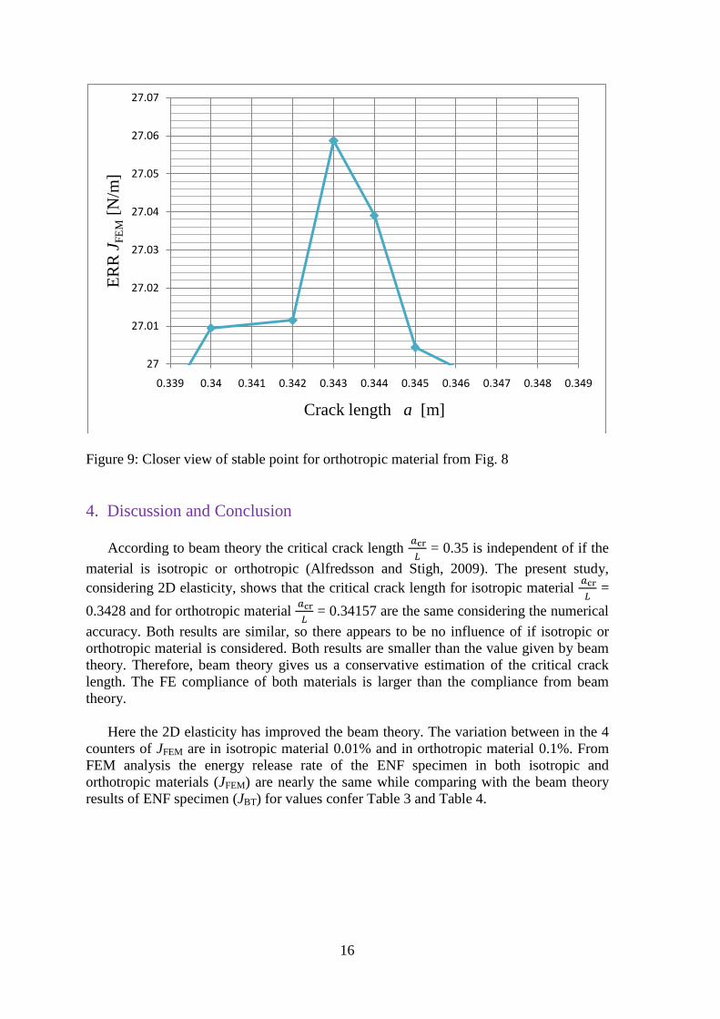
Figure 9: Closer view of stable point for orthotropic material from Fig. 8
4. Discussion and Conclusion
According to beam theory the critical crack length
= 0.35 is independent of if the
material is isotropic or orthotropic (Alfredsson and Stigh, 2009). The present study,
considering 2D elasticity, shows that the critical crack length for isotropic material
=
0.3428 and for orthotropic material
= 0.34157 are the same considering the numerical
accuracy. Both results are similar, so there appears to be no influence of if isotropic or
orthotropic material is considered. Both results are smaller than the value given by beam
theory. Therefore, beam theory gives us a conservative estimation of the critical crack
length. The FE compliance of both materials is larger than the compliance from beam
theory.
Here the 2D elasticity has improved the beam theory. The variation between in the 4
counters of JFEM are in isotropic material 0.01% and in orthotropic material 0.1%. From
FEM analysis the energy release rate of the ENF specimen in both isotropic and
orthotropic materials (JFEM) are nearly the same while comparing with the beam theory
results of ENF specimen (JBT) for values confer Table 3 and Table 4.
27
27.01
27.02
27.03
27.04
27.05
27.06
27.07
0.339 0.34 0.341 0.342 0.343 0.344 0.345 0.346 0.347 0.348 0.349
ER
R J
FE
M[N
/m]
Crack length a [m]
17
5. References
1) Alfredsson K.S. and Ulf Stigh. (2009). On the stability of beam like fracture
mechanics specimens. Manuscript in preparation.
2) Alfredsson K.S., Biel A. and Leffler K. (2003) An experimental method to determine
the complete stress-deformation relation for a structural adhesive layer loaded in
shear, In 9th International Conference on The Mechanical Behavior of Materials,
Geneva, Switzerland 2002
3) Anderson T.L. (2005) Fracture Mechanics Fundamentals And Applications. (3rd
ed.).
CRC press, NW.
4) Beer F.P. and Johnson E.R. (1992). Journal of Mechanics of Materials. (2nd
ed.).
McGraw-Hill, New York.
5) Broek D.(1984). Elementary engineering fracture mechanics: (3rd
ed.). The Hague:
Martinus Nijhoff Publishers
6) Carlsson L.A., Gillespie J.W. and Pipes R.B. (1986). On the analysis and design of the
end-notched flexure (ENF) specimens for mode II testing. Journal of Composites.
Mater.20, 594–605.
7) Chai H. (1988). Shear fracture. International Journal of Fracture. 37, 137-157.
8) Chai H. and Mall S. (1988). Design aspects of the end notch adhesive joint specimen.
International Journal of Fracture. 36, R3-R8.
9) Daniel I.M. and Ishai O. (1994). Engineering Mechanics of Composite Materials,
Oxford University Press, New York.
10) Irwin G.R. (1956). Onset of fast crack propagation in high strength steel and
aluminum alloys. Sagamore research conference proceedings. 2, 289 – 305.
11) Rice J. R. (1968) A path independent integral and the approximate analysis of strain
concentration by notches and cracks. Journal of applied mechanics. 35, 145 -153.
12) Robert D.C., David S.M., Michael E.P., Robert J.W. (2002) Concept And Applications
Of Finite Element Analysis (4th ed.). John Wiley & Sons. Inc. USA.
13) Russell A.J., Street K.N. (1982) A factor affecting the interlaminar fracture energy of
graphite/epoxy laminates. In: Hayashi T, Kawata K, Umekawa S, editors. Progress in
Science and Engineering of Composites, ICCM-IV, Tokyo, Japan 279–86
14) Wikipedia.org,(2010). J–Integral. Retrieved form internet.
http://en.wikipedia.org/wiki/J_integral.
Recommended