Statistical Statistical considerations for considerations for
grantsgrants
Brian HealyBrian Healy
Comments from previous Comments from previous classclass
Change time of courseChange time of course Available on-line power calculatorsAvailable on-line power calculators
– http://http://www.cs.uiowa.edu/~rlenth/Powerwww.cs.uiowa.edu/~rlenth/Power// Two-sided vs. one-sidedTwo-sided vs. one-sided Comparison of statistical packagesComparison of statistical packages
ReviewReview
Type I errorType I error Type II errorType II error Ways to increase powerWays to increase power Power/sample size calculation with Power/sample size calculation with
continuous outcomecontinuous outcome
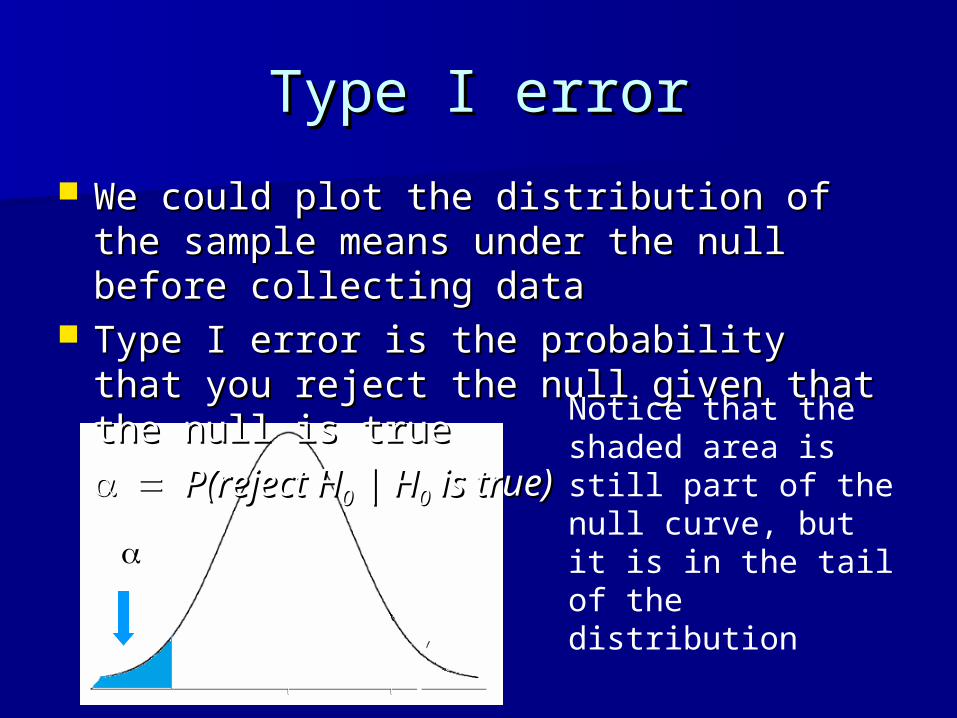
Type I errorType I error
We could plot the distribution of the We could plot the distribution of the sample means under the null before sample means under the null before collecting datacollecting data
Type I error is the probability that you Type I error is the probability that you reject the null given that the null is truereject the null given that the null is true
P(reject HP(reject H00 | H | H00 is true) is true)
Notice that the shaded area is still part of the null curve, but it is in the tail of the distribution
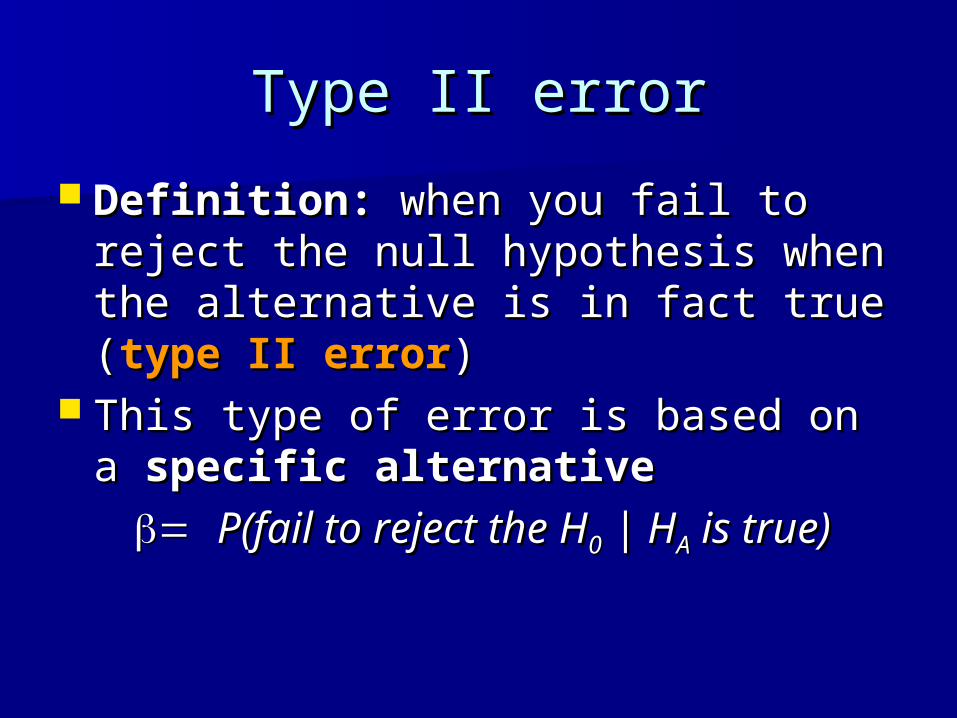
Type II errorType II error
Definition:Definition: when you fail to reject when you fail to reject the null hypothesis when the the null hypothesis when the alternative is in fact true (alternative is in fact true (type II type II errorerror))
This type of error is based on a This type of error is based on a specific alternativespecific alternative
P(fail to reject the HP(fail to reject the H00 | H | HAA is true) is true)
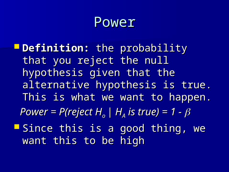
PowerPower
Definition:Definition: the probability that you the probability that you reject the null hypothesis given that reject the null hypothesis given that the alternative hypothesis is true. the alternative hypothesis is true. This is what we want to happen.This is what we want to happen.
Power = P(reject HPower = P(reject Ho o | H| HAA is true) = 1 - is true) = 1 - Since this is a good thing, we want Since this is a good thing, we want
this to be highthis to be high
OutlineOutline
Aspects of statistical considerations Aspects of statistical considerations section of a grantsection of a grant
Example statistical analysis sectionExample statistical analysis section Worked example from dataset from Worked example from dataset from
students in classstudents in class Management of data collection/ Management of data collection/
spreadsheetspreadsheet
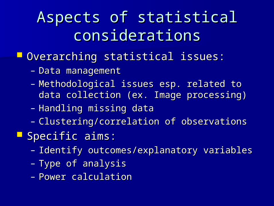
Aspects of statistical Aspects of statistical considerationsconsiderations
Overarching statistical issues:Overarching statistical issues:– Data managementData management– Methodological issues esp. related to data Methodological issues esp. related to data
collection (ex. Image processing)collection (ex. Image processing)– Handling missing dataHandling missing data– Clustering/correlation of observationsClustering/correlation of observations
Specific aims:Specific aims:– Identify outcomes/explanatory variablesIdentify outcomes/explanatory variables– Type of analysisType of analysis– Power calculationPower calculation
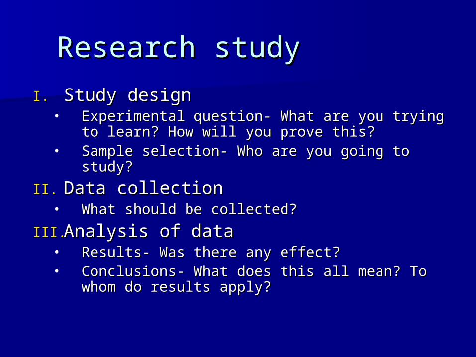
Research studyResearch study
I.I. Study designStudy design• Experimental question- What are you trying to Experimental question- What are you trying to
learn? How will you prove this?learn? How will you prove this?• Sample selection- Who are you going to study?Sample selection- Who are you going to study?
II.II. Data collectionData collection• What should be collected?What should be collected?
III.III. Analysis of dataAnalysis of data• Results- Was there any effect?Results- Was there any effect?• Conclusions- What does this all mean? To Conclusions- What does this all mean? To
whom do results apply?whom do results apply?
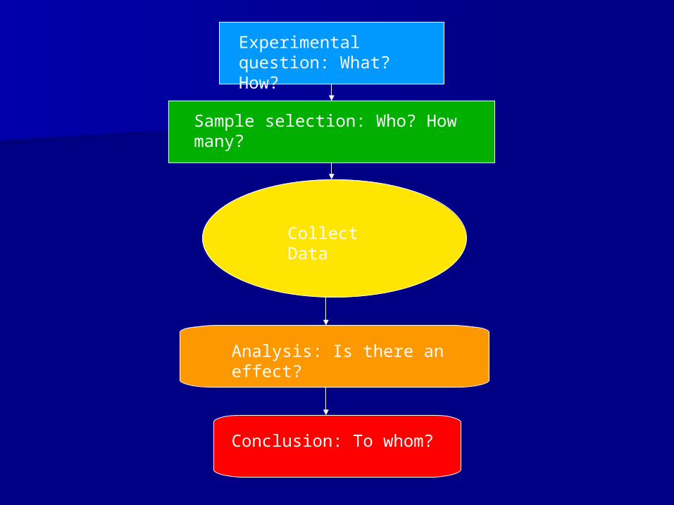
Experimental question: What? How?
Sample selection: Who? How many?
Collect Data
Analysis: Is there an effect?
Conclusion: To whom?
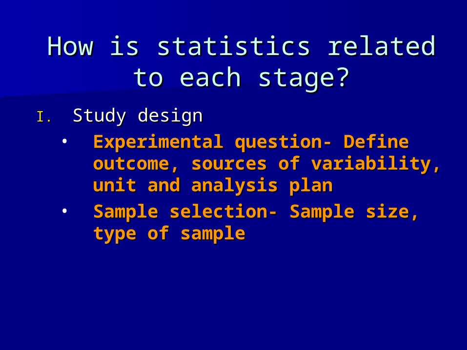
How is statistics related to each How is statistics related to each stage?stage?
I.I. Study designStudy design• Experimental question- Define Experimental question- Define
outcome, sources of variability, outcome, sources of variability, unit and analysis planunit and analysis plan
• Sample selection- Sample size, Sample selection- Sample size, type of sampletype of sample
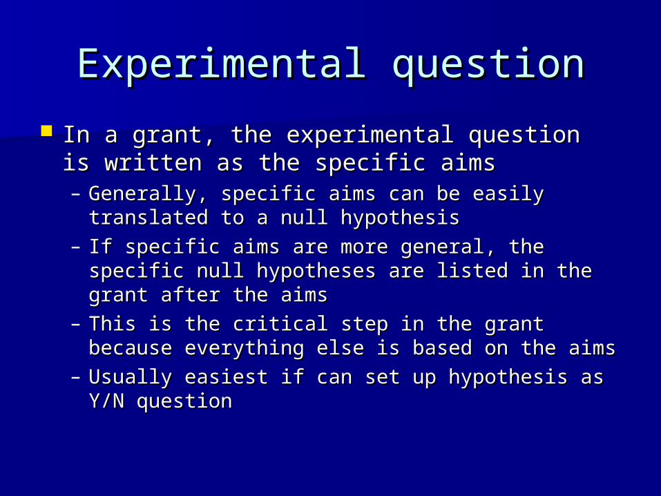
Experimental questionExperimental question
In a grant, the experimental question is In a grant, the experimental question is written as the specific aimswritten as the specific aims– Generally, specific aims can be easily Generally, specific aims can be easily
translated to a null hypothesistranslated to a null hypothesis– If specific aims are more general, the specific If specific aims are more general, the specific
null hypotheses are listed in the grant after the null hypotheses are listed in the grant after the aimsaims
– This is the critical step in the grant because This is the critical step in the grant because everything else is based on the aimseverything else is based on the aims
– Usually easiest if can set up hypothesis as Y/N Usually easiest if can set up hypothesis as Y/N questionquestion
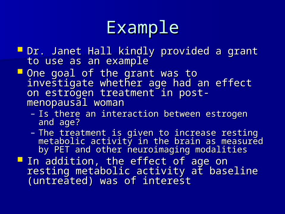
ExampleExample Dr. Janet Hall kindly provided a grant to Dr. Janet Hall kindly provided a grant to
use as an exampleuse as an example One goal of the grant was to investigate One goal of the grant was to investigate
whether age had an effect on estrogen whether age had an effect on estrogen treatment in post-menopausal womantreatment in post-menopausal woman– Is there an interaction between estrogen and Is there an interaction between estrogen and
age?age?– The treatment is given to increase resting The treatment is given to increase resting
metabolic activity in the brain as measured by metabolic activity in the brain as measured by PET and other neuroimaging modalitiesPET and other neuroimaging modalities
In addition, the effect of age on resting In addition, the effect of age on resting metabolic activity at baseline (untreated) metabolic activity at baseline (untreated) was of interestwas of interest
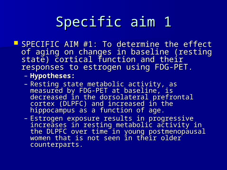
Specific aim 1Specific aim 1 SPECIFIC AIM #1: To determine the effect of SPECIFIC AIM #1: To determine the effect of
aging on changes in baseline (resting state) aging on changes in baseline (resting state) cortical function and their responses to cortical function and their responses to estrogen using FDG-PET.estrogen using FDG-PET.– Hypotheses: Hypotheses: – Resting state metabolic activity, as measured by Resting state metabolic activity, as measured by
FDG-PET at baseline, is decreased in the FDG-PET at baseline, is decreased in the dorsolateral prefrontal cortex (DLPFC) and dorsolateral prefrontal cortex (DLPFC) and increased in the hippocampus as a function of increased in the hippocampus as a function of age. age.
– Estrogen exposure results in progressive Estrogen exposure results in progressive increases in resting metabolic activity in the increases in resting metabolic activity in the DLPFC over time in young postmenopausal DLPFC over time in young postmenopausal women that is not seen in their older women that is not seen in their older counterparts. counterparts.
Hypothesis 1Hypothesis 1
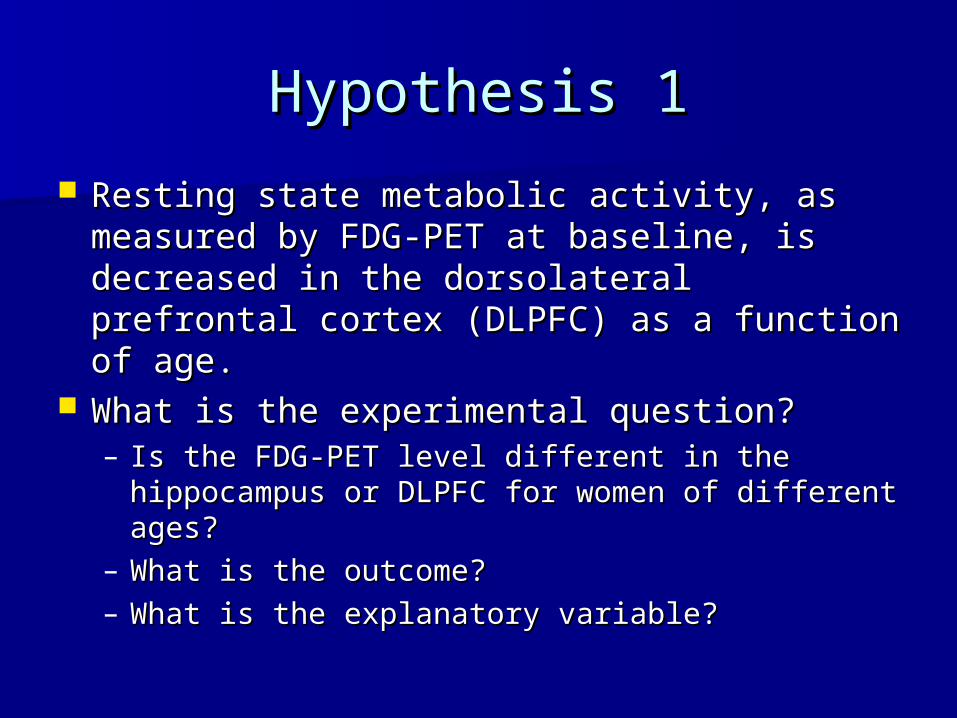
Resting state metabolic activity, as Resting state metabolic activity, as measured by FDG-PET at baseline, is measured by FDG-PET at baseline, is decreased in the dorsolateral prefrontal decreased in the dorsolateral prefrontal cortex (DLPFC) as a function of age.cortex (DLPFC) as a function of age.
What is the experimental question?What is the experimental question?– Is the FDG-PET level different in the Is the FDG-PET level different in the
hippocampus or DLPFC for women of different hippocampus or DLPFC for women of different ages?ages?
– What is the outcome?What is the outcome?– What is the explanatory variable?What is the explanatory variable?
Types of variablesTypes of variables
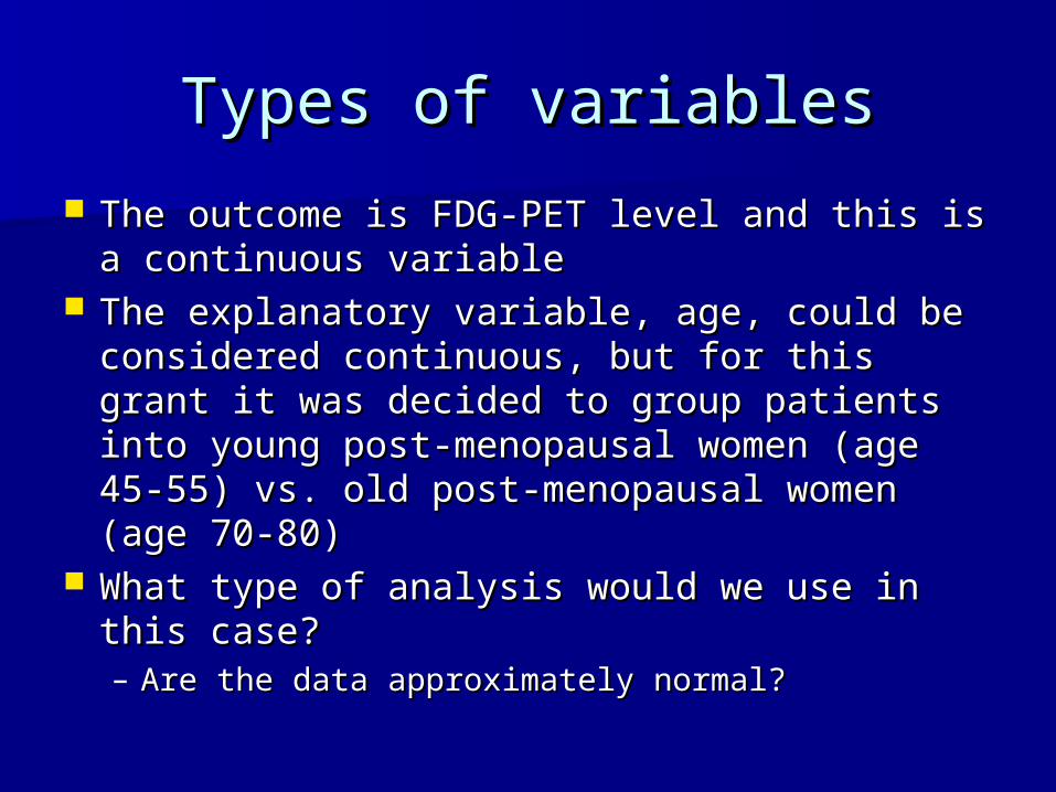
The outcome is FDG-PET level and this is a The outcome is FDG-PET level and this is a continuous variablecontinuous variable
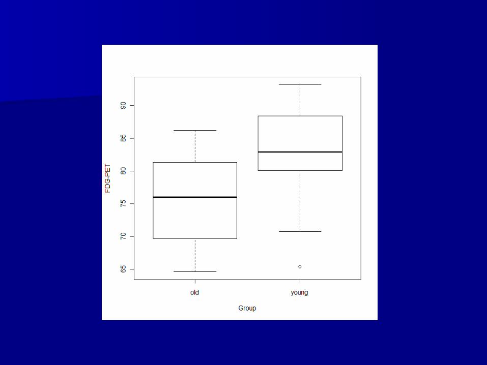
The explanatory variable, age, could be The explanatory variable, age, could be considered continuous, but for this grant it considered continuous, but for this grant it was decided to group patients into young was decided to group patients into young post-menopausal women (age 45-55) vs. post-menopausal women (age 45-55) vs. old post-menopausal women (age 70-80) old post-menopausal women (age 70-80)
What type of analysis would we use in this What type of analysis would we use in this case?case?– Are the data approximately normal?Are the data approximately normal?
Sample selectionSample selection
Our sample selection is based on the Our sample selection is based on the definition of the groupsdefinition of the groups– What is the effect of this definition? Does What is the effect of this definition? Does
it affect the generalizability of the it affect the generalizability of the findings?findings?
For this study, we plan to sample For this study, we plan to sample small groups from a single sitesmall groups from a single site– Could another approach have been used?Could another approach have been used?– What is the advantage of a single site? What is the advantage of a single site?
Disadvantage?Disadvantage?
Sample size calculationSample size calculation We have defined our null hypothesis, We have defined our null hypothesis,
outcome and sample selectionoutcome and sample selection What sample size do we need?What sample size do we need? In this case, previous data showed mean (SD) In this case, previous data showed mean (SD)
FDG-PET at DLPFC in the young group of 83.0 FDG-PET at DLPFC in the young group of 83.0 (7.3) and in the old group of 76.2 (7.3)(7.3) and in the old group of 76.2 (7.3)– What else do we need for our sample size What else do we need for our sample size
calculation?calculation?– Power=0.8, Power=0.8, =0.05=0.05
Assuming equal groups, we need 20 patients Assuming equal groups, we need 20 patients per groupper group
Additional considerationsAdditional considerations
Multiple comparisonsMultiple comparisons– We have two outcomes so should we We have two outcomes so should we
adjust the significance level for the two adjust the significance level for the two comparisons?comparisons?
– Bonferroni correction for significance Bonferroni correction for significance levellevel
Do any specifics regarding the Do any specifics regarding the measurement need to be discussed?measurement need to be discussed?
Confounders/adjustmentConfounders/adjustment
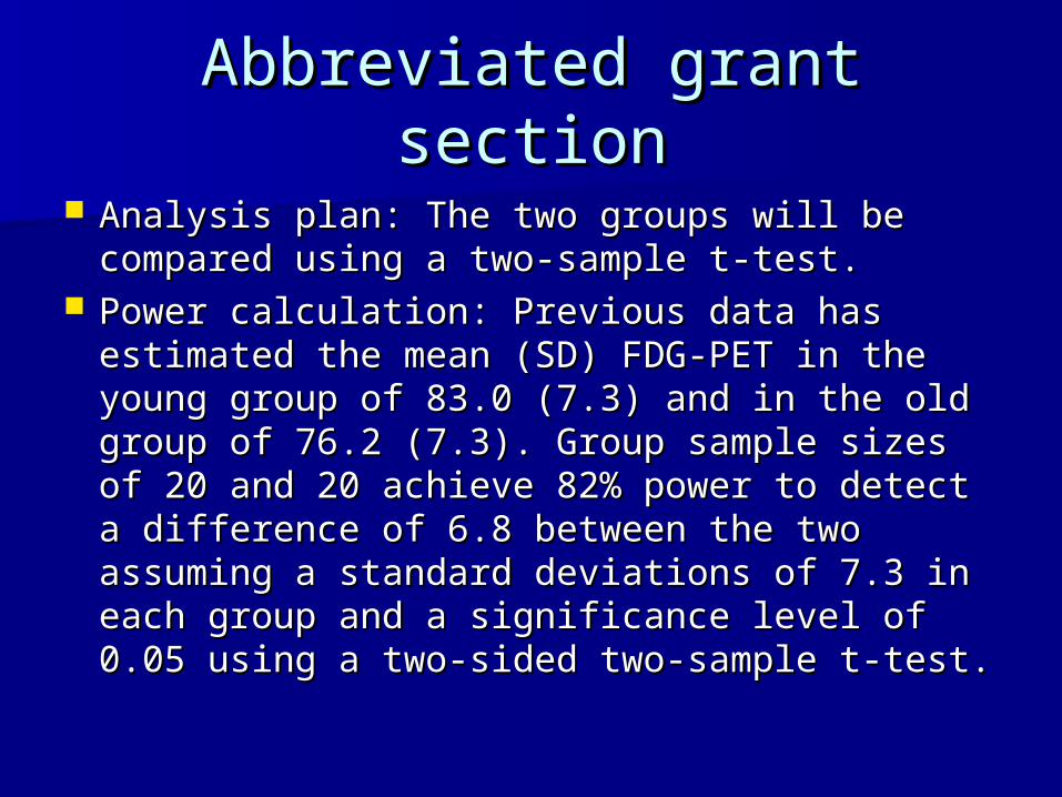
Abbreviated grant sectionAbbreviated grant section
Analysis plan: The two groups will be Analysis plan: The two groups will be compared using a two-sample t-test. compared using a two-sample t-test.
Power calculation: Previous data has Power calculation: Previous data has estimated the mean (SD) FDG-PET in the estimated the mean (SD) FDG-PET in the young group of 83.0 (7.3) and in the old young group of 83.0 (7.3) and in the old group of 76.2 (7.3). Group sample sizes of group of 76.2 (7.3). Group sample sizes of 20 and 20 achieve 82% power to detect a 20 and 20 achieve 82% power to detect a difference of 6.8 between the two assuming difference of 6.8 between the two assuming a standard deviations of 7.3 in each group a standard deviations of 7.3 in each group and a significance level of 0.05 using a two-and a significance level of 0.05 using a two-sided two-sample t-test.sided two-sample t-test.
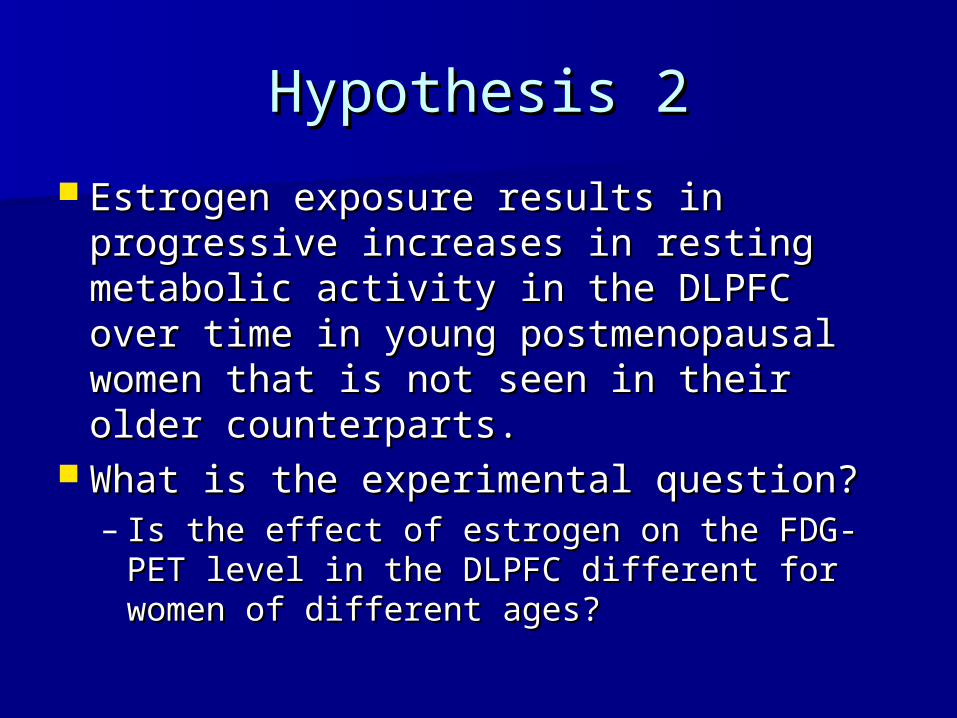
Hypothesis 2Hypothesis 2
Estrogen exposure results in Estrogen exposure results in progressive increases in resting progressive increases in resting metabolic activity in the DLPFC over metabolic activity in the DLPFC over time in young postmenopausal women time in young postmenopausal women that is not seen in their older that is not seen in their older counterparts. counterparts.
What is the experimental question?What is the experimental question?– Is the effect of estrogen on the FDG-PET Is the effect of estrogen on the FDG-PET
level in the DLPFC different for women of level in the DLPFC different for women of different ages?different ages?
Types of variablesTypes of variables
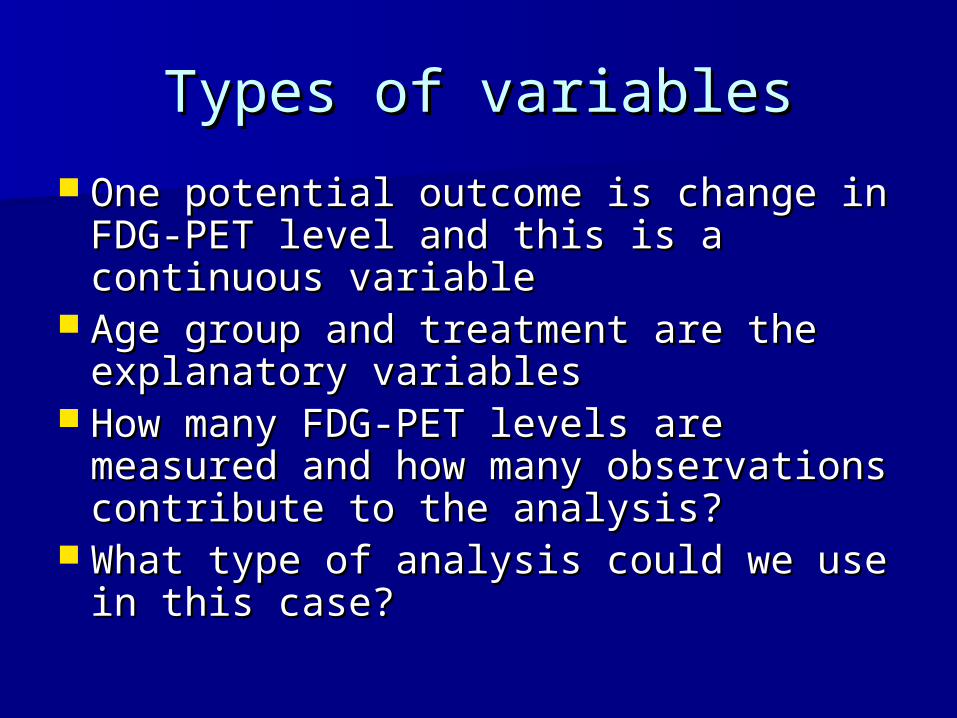
One potential outcome is change in One potential outcome is change in FDG-PET level and this is a continuous FDG-PET level and this is a continuous variablevariable
Age group and treatment are the Age group and treatment are the explanatory variablesexplanatory variables
How many FDG-PET levels are How many FDG-PET levels are measured and how many observations measured and how many observations contribute to the analysis?contribute to the analysis?
What type of analysis could we use in What type of analysis could we use in this case?this case?
Data set-upData set-up
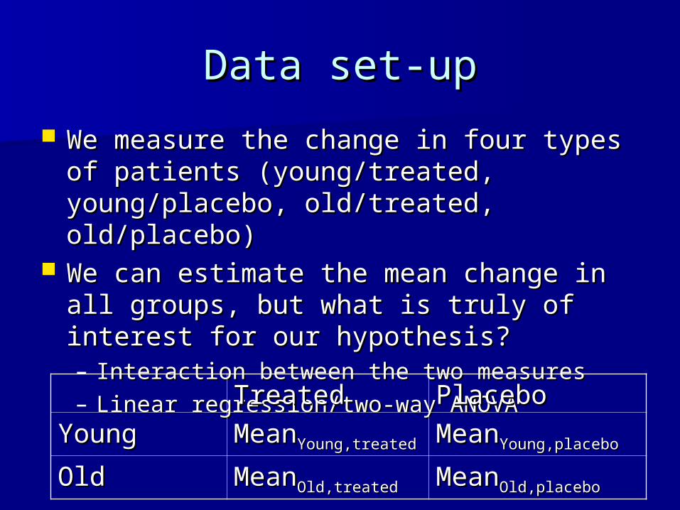
We measure the change in four types of We measure the change in four types of patients (young/treated, young/placebo, patients (young/treated, young/placebo, old/treated, old/placebo)old/treated, old/placebo)
We can estimate the mean change in all We can estimate the mean change in all groups, but what is truly of interest for our groups, but what is truly of interest for our hypothesis?hypothesis?– Interaction between the two measuresInteraction between the two measures– Linear regression/two-way ANOVALinear regression/two-way ANOVA
TreatedTreated PlaceboPlacebo
YoungYoung MeanMeanYoung,treatedYoung,treated MeanMeanYoung,placeboYoung,placebo
OldOld MeanMeanOld,treatedOld,treated MeanMeanOld,placeboOld,placebo
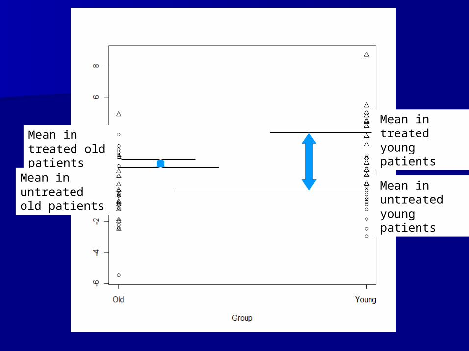
Mean in treated old patients
Mean in untreated old patients
Mean in untreated young patients
Mean in treated young patients
Sample selectionSample selection
Now that our outcome and Now that our outcome and explanatory variable are clearly explanatory variable are clearly defineddefined
Our sample selection in this case is a Our sample selection in this case is a little more complexlittle more complex– Age group is defined by enrollmentAge group is defined by enrollment– Patients in each group were randomized Patients in each group were randomized
to treatment or placeboto treatment or placebo– What does the randomization get for us?What does the randomization get for us?
Sample size calculationSample size calculation
We have defined our null hypothesis, We have defined our null hypothesis, outcome and sample selectionoutcome and sample selection
What sample size do we need?What sample size do we need?– What preliminary data would we need or What preliminary data would we need or
what would we need to hypothesize to what would we need to hypothesize to calculate the sample size?calculate the sample size?
Some resources for this complex Some resources for this complex design on-line, but likely you should design on-line, but likely you should consider speaking to a statistician for consider speaking to a statistician for thisthis
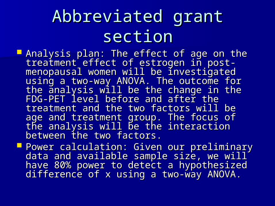
Abbreviated grant sectionAbbreviated grant section Analysis plan: The effect of age on the Analysis plan: The effect of age on the
treatment effect of estrogen in post-treatment effect of estrogen in post-menopausal women will be investigated menopausal women will be investigated using a two-way ANOVA. The outcome for using a two-way ANOVA. The outcome for the analysis will be the change in the FDG-the analysis will be the change in the FDG-PET level before and after the treatment and PET level before and after the treatment and the two factors will be age and treatment the two factors will be age and treatment group. The focus of the analysis will be the group. The focus of the analysis will be the interaction between the two factors. interaction between the two factors.
Power calculation: Given our preliminary Power calculation: Given our preliminary data and available sample size, we will have data and available sample size, we will have 80% power to detect a hypothesized 80% power to detect a hypothesized difference of x using a two-way ANOVA.difference of x using a two-way ANOVA.
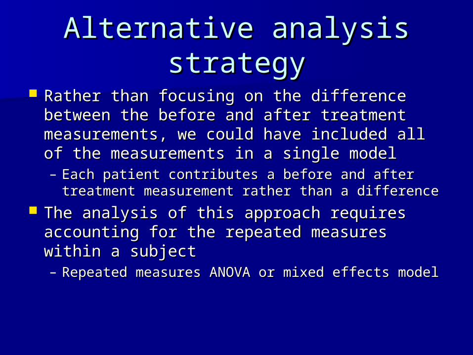
Alternative analysis strategyAlternative analysis strategy
Rather than focusing on the difference Rather than focusing on the difference between the before and after treatment between the before and after treatment measurements, we could have included all of measurements, we could have included all of the measurements in a single modelthe measurements in a single model– Each patient contributes a before and after Each patient contributes a before and after
treatment measurement rather than a differencetreatment measurement rather than a difference The analysis of this approach requires The analysis of this approach requires
accounting for the repeated measures within accounting for the repeated measures within a subjecta subject– Repeated measures ANOVA or mixed effects Repeated measures ANOVA or mixed effects
modelmodel
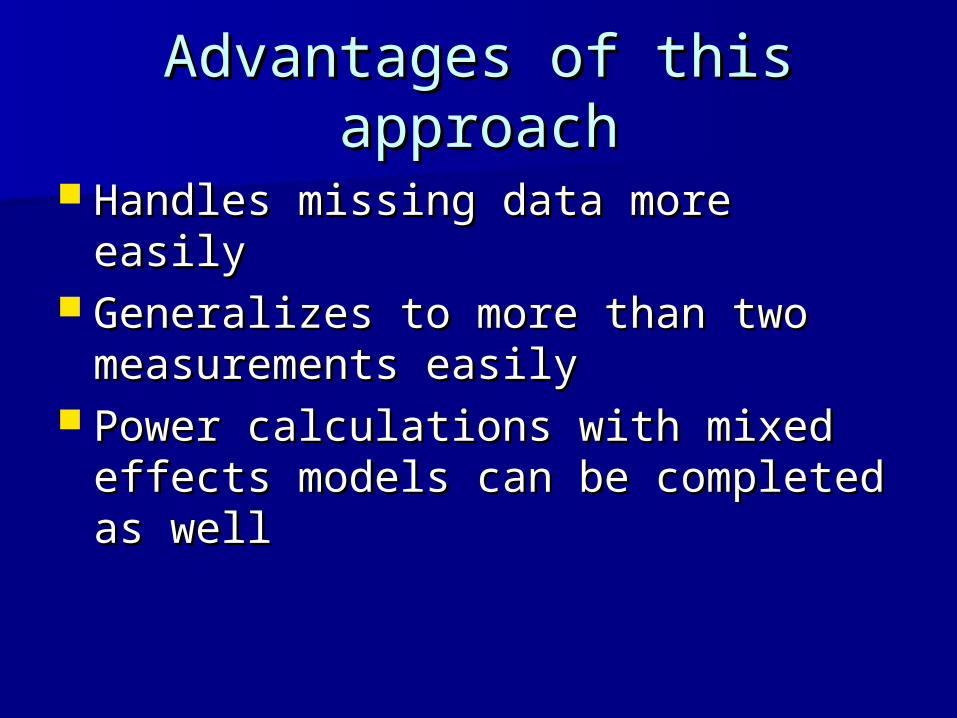
Advantages of this approachAdvantages of this approach
Handles missing data more easilyHandles missing data more easily Generalizes to more than two Generalizes to more than two
measurements easilymeasurements easily Power calculations with mixed effects Power calculations with mixed effects
models can be completed as wellmodels can be completed as well

ConclusionsConclusions
Each hypothesis needs an analysis Each hypothesis needs an analysis plan that describes the type of data plan that describes the type of data and statistical approach used to and statistical approach used to analyze the dataanalyze the data
Each hypothesis also requires a Each hypothesis also requires a sample size or power calculationsample size or power calculation
Additional issues (missing data, Additional issues (missing data, confounding) must be included in the confounding) must be included in the statistical analysis sectionstatistical analysis section
Worked exampleWorked example
Kidney transplant researchKidney transplant research
Students in the class are investigating the Students in the class are investigating the effect of genetics of the donor/recipient effect of genetics of the donor/recipient pair on various outcomespair on various outcomes– Creatinine level measured at time of Creatinine level measured at time of
transplant, 3 month, 6 month, 12 month and transplant, 3 month, 6 month, 12 month and 36 months after transplant36 months after transplant
– Time to rejection of the transplantTime to rejection of the transplant– Type of rejection (acute/chronic)Type of rejection (acute/chronic)
Genetic factor of interest is large deletion Genetic factor of interest is large deletion polymorphisms at 20 sitespolymorphisms at 20 sites
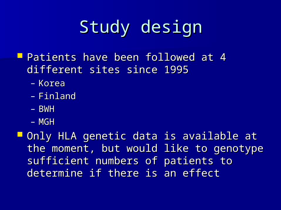
Study designStudy design
Patients have been followed at 4 different Patients have been followed at 4 different sites since 1995sites since 1995– KoreaKorea– FinlandFinland– BWHBWH– MGHMGH
Only HLA genetic data is available at the Only HLA genetic data is available at the moment, but would like to genotype moment, but would like to genotype sufficient numbers of patients to sufficient numbers of patients to determine if there is an effectdetermine if there is an effect
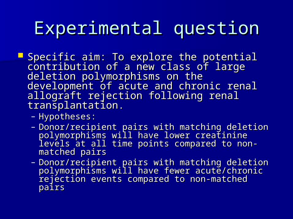
Experimental questionExperimental question Specific aim: To explore the potential Specific aim: To explore the potential
contribution of a new class of large deletion contribution of a new class of large deletion polymorphisms on the development of acute polymorphisms on the development of acute and chronic renal allograft rejection following and chronic renal allograft rejection following renal transplantation. renal transplantation. – Hypotheses:Hypotheses:– Donor/recipient pairs with matching deletion Donor/recipient pairs with matching deletion
polymorphisms will have lower creatinine levels at polymorphisms will have lower creatinine levels at all time points compared to non-matched pairs all time points compared to non-matched pairs
– Donor/recipient pairs with matching deletion Donor/recipient pairs with matching deletion polymorphisms will have fewer acute/chronic polymorphisms will have fewer acute/chronic rejection events compared to non-matched pairs rejection events compared to non-matched pairs
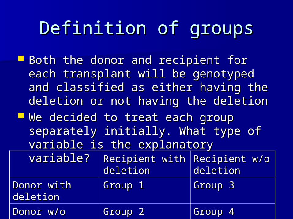
Definition of groupsDefinition of groups
Both the donor and recipient for each Both the donor and recipient for each transplant will be genotyped and classified transplant will be genotyped and classified as either having the deletion or not having as either having the deletion or not having the deletionthe deletion
We decided to treat each group separately We decided to treat each group separately initially. What type of variable is the initially. What type of variable is the explanatory variable?explanatory variable?
Recipient with Recipient with deletiondeletion
Recipient w/o Recipient w/o deletiondeletion
Donor with Donor with deletiondeletion
Group 1Group 1 Group 3Group 3
Donor w/o Donor w/o deletiondeletion
Group 2Group 2 Group 4Group 4
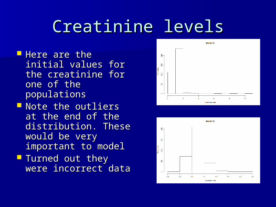
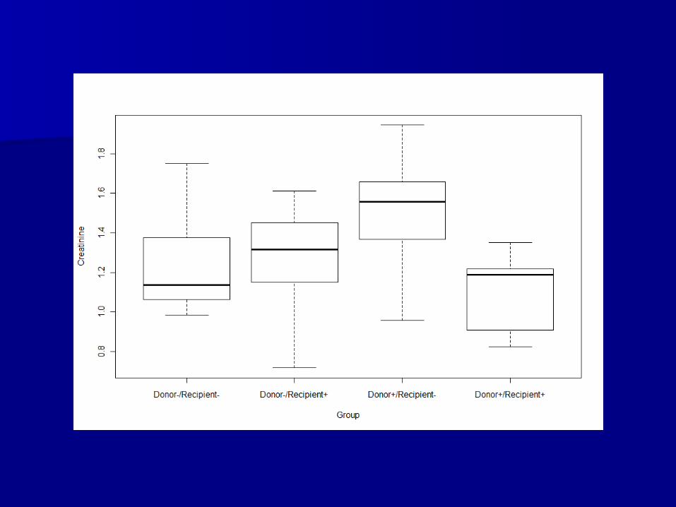
Creatinine levelsCreatinine levels Here are the initial Here are the initial
values for the values for the creatinine for one creatinine for one of the populationsof the populations
Note the outliers at Note the outliers at the end of the the end of the distribution. These distribution. These would be very would be very important to modelimportant to model
Turned out they Turned out they were incorrect data were incorrect data
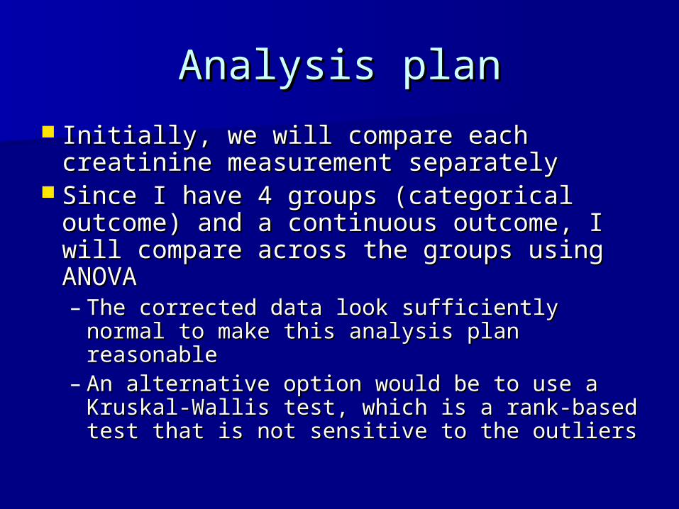
Analysis planAnalysis plan
Initially, we will compare each Initially, we will compare each creatinine measurement separatelycreatinine measurement separately
Since I have 4 groups (categorical Since I have 4 groups (categorical outcome) and a continuous outcome, I outcome) and a continuous outcome, I will compare across the groups using will compare across the groups using ANOVAANOVA– The corrected data look sufficiently normal The corrected data look sufficiently normal
to make this analysis plan reasonableto make this analysis plan reasonable– An alternative option would be to use a An alternative option would be to use a
Kruskal-Wallis test, which is a rank-based Kruskal-Wallis test, which is a rank-based test that is not sensitive to the outlierstest that is not sensitive to the outliers
Abbreviated analysis planAbbreviated analysis plan Analysis plan: The four groups of Analysis plan: The four groups of
donor/recipient pairs will be compared donor/recipient pairs will be compared using ANOVA. If a significant difference using ANOVA. If a significant difference between the groups is observed, the between the groups is observed, the pairwise comparisons will be completed pairwise comparisons will be completed with the appropriate correction for multiple with the appropriate correction for multiple comparisons. Although we could investigate comparisons. Although we could investigate the main effect of the donor’s and the main effect of the donor’s and recipient’s deletion status in a two-way recipient’s deletion status in a two-way ANOVA model, our interest is in the four ANOVA model, our interest is in the four group comparison given the relationships group comparison given the relationships seen in previous work. seen in previous work.
Additional considerationsAdditional considerations
Rather than modeling each creatinine Rather than modeling each creatinine separately, should we model them separately, should we model them together?together?– Trend with time?Trend with time?– Multiple comparisons if treat separately?Multiple comparisons if treat separately?
Confounders:Confounders:– AgeAge– GenderGender– HLA statusHLA status
Should we treat all 20 deletion separately?Should we treat all 20 deletion separately?
Power calculationPower calculation
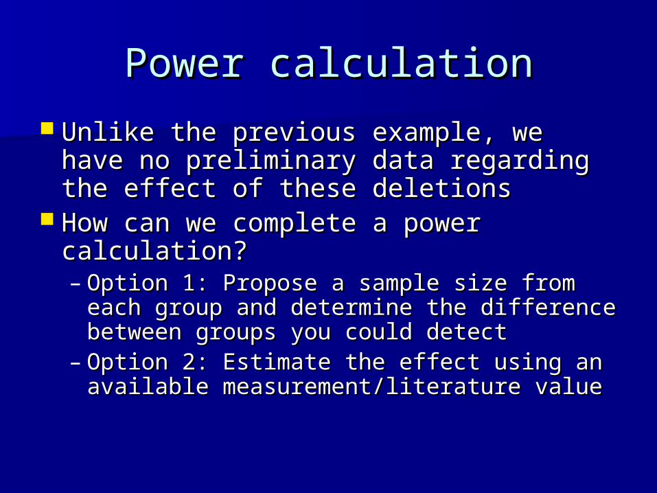
Unlike the previous example, we Unlike the previous example, we have no preliminary data regarding have no preliminary data regarding the effect of these deletionsthe effect of these deletions
How can we complete a power How can we complete a power calculation?calculation?– Option 1: Propose a sample size from Option 1: Propose a sample size from
each group and determine the difference each group and determine the difference between groups you could detectbetween groups you could detect
– Option 2: Estimate the effect using an Option 2: Estimate the effect using an available measurement/literature valueavailable measurement/literature value
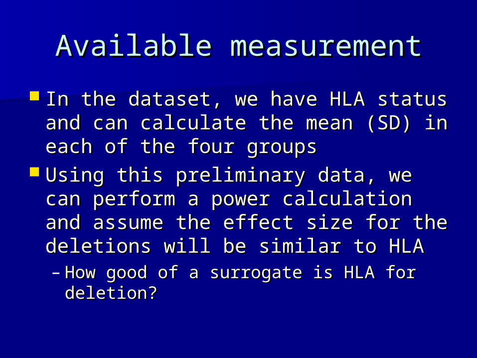
Available measurementAvailable measurement
In the dataset, we have HLA status In the dataset, we have HLA status and can calculate the mean (SD) in and can calculate the mean (SD) in each of the four groupseach of the four groups
Using this preliminary data, we can Using this preliminary data, we can perform a power calculation and perform a power calculation and assume the effect size for the assume the effect size for the deletions will be similar to HLAdeletions will be similar to HLA– How good of a surrogate is HLA for How good of a surrogate is HLA for
deletion?deletion?
Abbreviated power Abbreviated power calculationcalculation
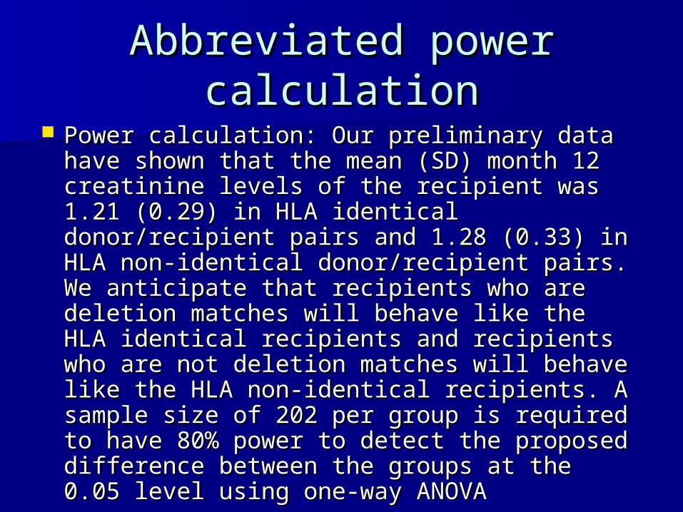
Power calculation: Our preliminary data Power calculation: Our preliminary data have shown that the mean (SD) month 12 have shown that the mean (SD) month 12 creatinine levels of the recipient was 1.21 creatinine levels of the recipient was 1.21 (0.29) in HLA identical donor/recipient pairs (0.29) in HLA identical donor/recipient pairs and 1.28 (0.33) in HLA non-identical and 1.28 (0.33) in HLA non-identical donor/recipient pairs. We anticipate that donor/recipient pairs. We anticipate that recipients who are deletion matches will recipients who are deletion matches will behave like the HLA identical recipients and behave like the HLA identical recipients and recipients who are not deletion matches will recipients who are not deletion matches will behave like the HLA non-identical recipients. behave like the HLA non-identical recipients. A sample size of 202 per group is required to A sample size of 202 per group is required to have 80% power to detect the proposed have 80% power to detect the proposed difference between the groups at the 0.05 difference between the groups at the 0.05 level using one-way ANOVAlevel using one-way ANOVA
Additional considerationsAdditional considerations
Pairwise testsPairwise tests Is there a better approximation for Is there a better approximation for
the group means?the group means? Clustering by countryClustering by country
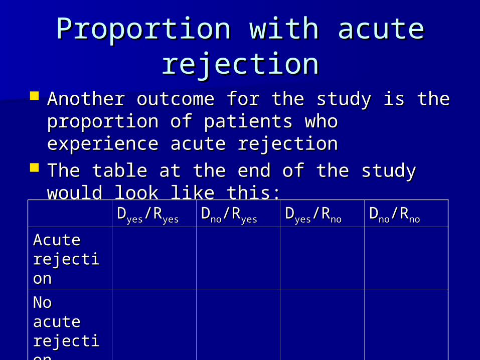
Proportion with acute Proportion with acute rejectionrejection
Another outcome for the study is the Another outcome for the study is the proportion of patients who experience proportion of patients who experience acute rejectionacute rejection
The table at the end of the study would The table at the end of the study would look like this:look like this:
DDyesyes/R/Ryesyes DDnono/R/Ryesyes DDyesyes/R/Rnono DDnono/R/Rnono
Acute Acute rejectionrejection
No acute No acute rejectionrejection
Abbreviated analysis planAbbreviated analysis plan
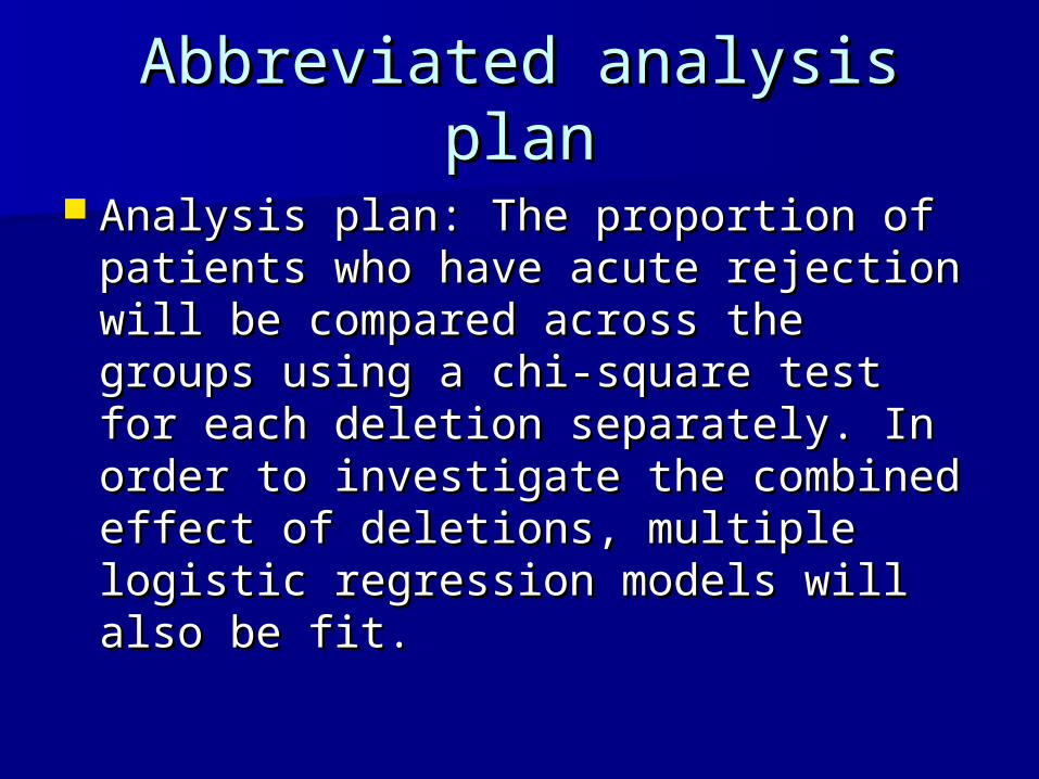
Analysis plan: The proportion of Analysis plan: The proportion of patients who have acute rejection patients who have acute rejection will be compared across the groups will be compared across the groups using a chi-square test for each using a chi-square test for each deletion separately. In order to deletion separately. In order to investigate the combined effect of investigate the combined effect of deletions, multiple logistic regression deletions, multiple logistic regression models will also be fit.models will also be fit.
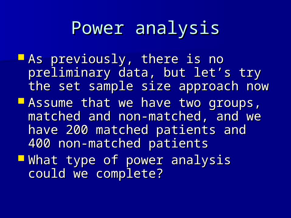
Power analysisPower analysis
As previously, there is no preliminary As previously, there is no preliminary data, but let’s try the set sample size data, but let’s try the set sample size approach nowapproach now
Assume that we have two groups, Assume that we have two groups, matched and non-matched, and we matched and non-matched, and we have 200 matched patients and 400 have 200 matched patients and 400 non-matched patientsnon-matched patients
What type of power analysis could What type of power analysis could we complete?we complete?
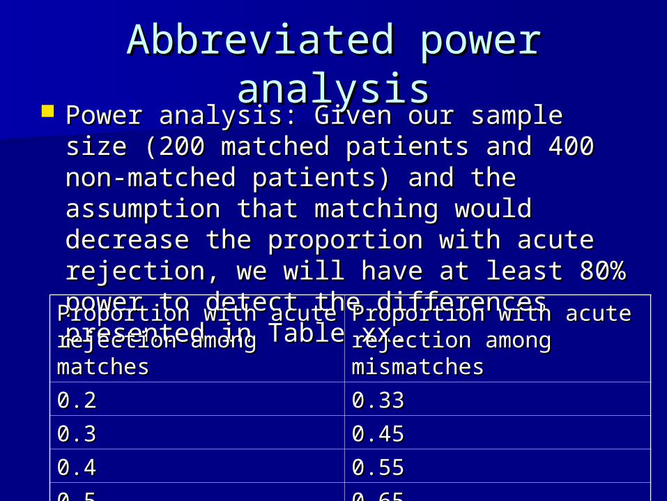
Abbreviated power analysisAbbreviated power analysis Power analysis: Given our sample size Power analysis: Given our sample size
(200 matched patients and 400 non-(200 matched patients and 400 non-matched patients) and the assumption matched patients) and the assumption that matching would decrease the that matching would decrease the proportion with acute rejection, we will proportion with acute rejection, we will have at least 80% power to detect the have at least 80% power to detect the differences presented in Table xx.differences presented in Table xx.Proportion with acute Proportion with acute
rejection among rejection among matchesmatches
Proportion with acute Proportion with acute rejection among rejection among mismatchesmismatches
0.20.2 0.330.33
0.30.3 0.450.45
0.40.4 0.550.55
0.50.5 0.650.65
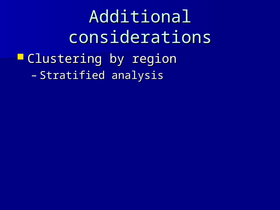
Additional considerationsAdditional considerations
Clustering by regionClustering by region– Stratified analysisStratified analysis
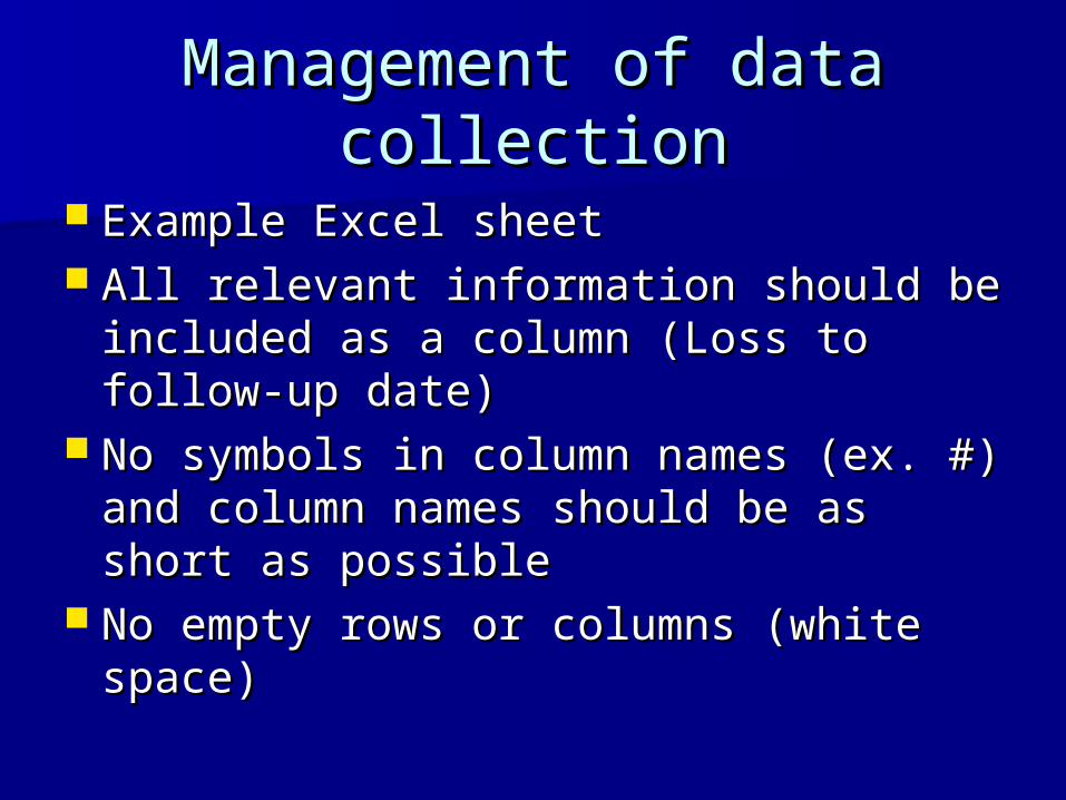
Management of data Management of data collectioncollection
Example Excel sheetExample Excel sheet All relevant information should be All relevant information should be
included as a column (Loss to follow-included as a column (Loss to follow-up date)up date)
No symbols in column names (ex. #) No symbols in column names (ex. #) and column names should be as short and column names should be as short as possibleas possible
No empty rows or columns (white No empty rows or columns (white space)space)
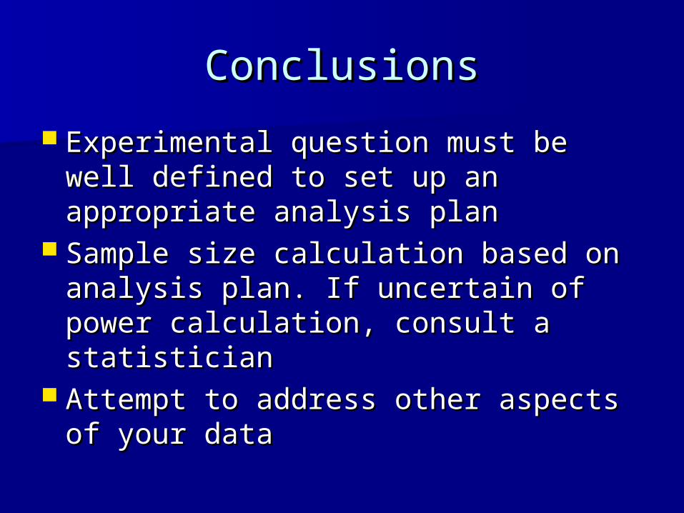
ConclusionsConclusions
Experimental question must be well Experimental question must be well defined to set up an appropriate defined to set up an appropriate analysis plananalysis plan
Sample size calculation based on Sample size calculation based on analysis plan. If uncertain of power analysis plan. If uncertain of power calculation, consult a statisticiancalculation, consult a statistician
Attempt to address other aspects of Attempt to address other aspects of your datayour data

THANK YOU!!!THANK YOU!!!
Recommended