D.P. Lovell May 2013 1
Draft report on Statistical issues related to OECD in vitro genotoxicity Test
Guidelines
Note:
This document has been used to support the revision of draft Test Guidelines 473 and
487. Thus the new versions of TGs 473 and 487 (dated September 2013, for review by
the WNT from 20 September until 4 November 2013) are not the versions of the TGs
the consultant for the Secretariat in charge of the development of the report worked
from. The report might thus refer to some text of the TGs that is not included anymore
in the current versions. Wording will be adapted, where necessary, to fix this in the
final version of the report.
Summary
1. This report explores a number of statistical issues related to OECD guidelines for
genotoxicity. Firstly, a review of previous work investigating the optimal number
of cells and animals needed for the in vivo micronucleus test (TG 474). Secondly,
analyses related to statistical issues associated with TG 473 (in vitro chromosomal
aberration test) and TG 487 (in vitro micronucleus test).
2. The results of two investigations by Kissling et al and Health Canada (HC) were
reviewed and together with various further simulations it was concluded that the
methods were in broad agreement, that studies with sample sizes of 5 and scoring
4000 cells per animal had approximately 80% power to detect about 2-3 fold
increases when the negative control incidence was high but that the power was
smaller for lower background levels.
3. A number of laboratories provided historical negative control data for the in vitro
cytogenetics (21 laboratories) and micronuclei (15 laboratories) tests. The
distributions of the aberrations and micronuclei were derived for these samples.
4. There was no clear distinction between the mean scores for the different cell
types. The range of variability in the chromosomal aberrations was relatively
narrow but wider for the in vitro micronucleus tests. While there was variability
between laboratories, there was little evidence for differences in incidence
depending upon the presence or absence of S9 mix or different treatment times.
5. Combining data from replicate negative control cultures would provide an
increase in power. Scoring more cells from the concurrent negative control would
also provide slightly more power and more consistent results. Using more
concentration levels would provide a more accurate description of the
concentration-response relationship. A trend test is more powerful than pair-wise
comparisons especially if multiple comparison procedures are applied.
6. Similar power calculations were done for the two tests. These showed that the in
vitro chromosomal aberration test had low power to detect a 2-fold increase. The
power curves that were derived provide indications of the number of cells that
would be needed to identify a fold increase or, alternatively, the power associated
with various designs.

D.P. Lovell May 2013 2
7. There was no evidence in the datasets provided that there was heterogeneity
between replicate cultures but a number of laboratories showed appreciable
between experiment variability.
8. In the absence of inter-replicate variability the in vitro micronucleus test has
power comparable with the in vivo micronucleus test but in the presence of inter-
replicate variability it may be vulnerable to artifactual results. The use of more
replicate cultures may provide some protection against possible artifactual results
if the number of cell counted per concentration levels were to be greatly increased.
9. Although it was concluded that the datasets were adequate for carrying out the
investigations it was noted that some improvements could be made to the
development of databases of negative control data.
10. In response to further questions, the numbers of cells needed to be scored in some
of the tests to avoid zero counts was explored. Based upon a Poisson distribution,
samples where sufficient cells were measured such that the mean culture counts
were approximately 5 would result in only a few cultures having scores of zero
and the data would be approximately normally distributed. This would provide
data that would be convenient for statistical analysis but this is not a prerequisite
to achieving an adequate statistical analysis.
11. Eight scenarios for the use of historical negative control data to help determine a
positive result and in the assessment of the biological importance of the results
were explored. Most methods have some limitations. The GEF (Global
Equivalence Factor) approach used in the Mouse Lymphoma Assay (MLA) test
may have some potential. Another approach that might warrant further
investigation is to use C-charts, developed for quality control purposes. These
together with control limits based upon the Poisson distribution could provide an
indication of results that would not be considered unusual as well as those which
would indicate an effect had occurred.
Introduction
12. The purpose of this work was to perform statistical analyses to support the
determination of the optimal number of cells to be scored in Test Guideline (TG)
473 (in vitro chromosomal aberration test), TG 476 and TG 476 bis (in vitro gene
mutation tests) and TG 487 (in vitro micronucleus test), after reviewing and taking
into consideration approaches already developed for determining the statistical
power of the Erythrocyte Micronucleus Assay (TG 474) and in vivo chromosomal
aberration assay (TG 475).
13. This report reviews analyses previously carried out with respect to the in vivo
micronucleus test (TG 474) and then discusses statistical issues associated with
Test Guidelines (TGs 473 and 487).

D.P. Lovell May 2013 3
Some general points related to in vitro study designs and their statistical analysis
Hierarchical / nested designs
14. Many genotoxicity designs such as the in vivo and in vitro cytogenetics or
micronucleus assays are hierarchical or nested designs in that there are cultures or
animals 'nested' within treatment groups and a number of cells from each animal
or culture are scored. The different levels in the design have differing degrees of
variation which ideally should be taken into account in any statistical analysis.
15. A key concept in the statistical analysis of a hierarchical design is the
identification of the experimental unit. This is defined as the "smallest amount of
experimental material that can be randomly assigned to a treatment”. In principle,
this should be the culture or the animal as it is impractical in the test to assign cells
randomly from the same animal or culture to different treatment groups.
16. There may be differences between cultures within a concentration level and
between cells within a culture. The cells within a culture, however, are not
independent and correlations between cells can lead to biases. In general,
statistical analyses should take into account these different levels of variability
otherwise ‘hidden’ levels of variability may distort estimates of variability and
lead to errors in interpretation.
17. Statistical tests which appear more powerful may be carried out by analyzing the
data at the cell level rather than the culture level. This apparent increase in sample
size is an example of pseudo-replication where there are no true replications of the
observations because repeated measurements of the same sample are wrongly
treated as independent. This is a violation of an important assumption underlying
statistical analyses such as the Chi-square and Fisher's exact tests of 2 x 2 tables
which assumes that the individual data points to be analysed are independent of
one another. In effect, measuring more and more cells from the same animal or
culture can result in a more precise description of that unit and the apparent
identification of increasingly significant differences between animals or cultures
as the number of cells is increased, leading to an overestimation of the statistical
significance of comparisons
18. Clearly, in many in vitro tests the experimental unit would be the culture and the
test could, therefore, be severely underpowered. However, the genotoxicity
'community' is aware of these potential limitations as well as the degree of inter-
culture variability in their tests. It uses its considerable experience and
understanding of the test systems to take a pragmatic approach to the analysis and
interpretation of the assay results.
Limitations of Power calculations
19. The power of a study is the probability of detecting a true effect of a specific size
or larger using a particular statistical test at a specific probability level. The power
is (1-β) where β is the Type II error associated with a hypothesis test. (The Type II
error is the probability of wrongly accepting the null hypothesis as true when it is

D.P. Lovell May 2013 4
actually false while the Type I error is the probability of rejecting the null
hypothesis when it is actually true.)
20. Power and sample size calculations are an important part of the design of
experiments and have an important role in identifying the feasibility of a design
and identifying the resources needed to ensure a successful outcome.
21. These calculations depend upon the formulation of a null and alternative
hypothesis and can be easy to carry out when there are just one or two treatment
groups using closed form equations which are now available in many software
packages. More sophisticated designs require simulations involving the use of
pseudo-random numbers to mimic experimental results.
22. It is, though, important to appreciate the limitations of these methods which are
dependent upon the assumptions and inputs into the equations and simulations.
They are based around the use of P-values for statistical inference and the
identification of 'statistically significant' results, an approach which is under
considerable criticism in the statistical literature and the increasing appreciation
that statistical significance does not equate to biological importance.
23. Power calculations are also very dependent upon the estimate of the standard
deviations included in the calculations. Estimates of the measure of variability
have their own variability and the variance of an estimate of the variance/standard
deviation can be large so that estimates of sample sizes are vulnerable to these
assumptions.
24. Table 1 shows the 95% confidence intervals for the estimates of variability in the
Kissling et al's (2007) paper. This shows that when the sample sizes are smallish
(i.e. less than 30) that the upper confidence limit can be twice as big as the lower
one. The implication here is that this variability can affect the sample sizes needed
to equate the binomial counting error to the inter-animal variability.
25. An experimental result is a sample of one from the population of all the possible
experiments of the same design that could have been done. This single result is,
therefore, somewhere on the hypothetical distribution of possible results and gives
the ‘best’ estimate of the true state. In practice, it could be very close to the true or
expected value, but it could also be near the upper extreme of the distribution of a
low effect or the lower end of a high difference. It is not possible to distinguish
from this single result which is correct.
26. One consequence of a design with 80% power is that it will also be able to detect
effects smaller than the specified effect but with lower power. The design will
then be capable of detecting real but small effects, which while being statistically
significant are considered biologically unimportant (i.e. a negative ‘call’). A study
which is designed to have 80% power to detect a specified effect will also have,
for instance, 50% power to detect a smaller effect. This particular effect is also the
effect that will be just statistically significant at the chosen critical value say
P=0.05.

D.P. Lovell May 2013 5
1) Consideration of approaches developed for determining statistical power of
the Erythrocyte Micronucleus Assay (TG 474)
27. The objective of the section is to review and comment on the analyses that have
been done by Kissling et al (2007) and Health Canada (HC) (2012) in the context
of the revision of in vivo genotoxicity Test Guidelines.
28. In the in vivo micronucleus assay (TG 474) some discussions has centred on
recommendations to design studies with two specific characteristics. Firstly, to
have sufficient power to be able to detect a fold increase (or doubling) of the
endpoint. Secondly, to identify the number of cells that needs to be scored to
reduce the binomial error to that of the inter-animal variability.
29. An objective of Kissling et al's (2007) work was to equate the “counting error” to
the “inter-animal variability”. They combined the binomial counting error
expressed as a coefficient of variation (CV) with the inter-animal CV to obtain an
expression giving n, the sample sizes of cells needed to equate the two measures.
These two terms, respectively, are equated to the %CVs in their Table 2 and the %
CVs in their Table 1.
Kissling et al's (Table 1) of mean and SD of various groups
% n SD CV%
Rat 0.11 15 0.05 41
Rat 0.23 190 0.06 26
Mouse 0.20 79 0.20 35
Dog 0.31 22 0.31 30
30. Kissling et al (2007) equate the "binomial counting error" to the standard error
(also called the standard deviation) of the binomial distribution of a proportion
assuming such a distribution.
31. Kissling et al (2007) also carried out a Monte Carlo simulation to investigate the
properties of the design in terms of statistical power. One-tailed non-parametric
Mann-Whitney tests were carried out to make comparisons between the 'control'
and 'treated' groups.
32. They introduced inter-animal variability by simulating inter-animal differences
from a distribution with a defined mean and SD based upon 4 combinations of
representative values of percentages and SD (from their Table 1) and identified
fold increases that could be identified. Individual micronuclei frequencies for
each of the 10 animals were derived based upon the binomial distribution for
2000, 4000 and 20000 cells. 3000 runs were carried out with increasing levels of
fold increase (f) until the 'power' exceeded either 90 or 95%. (Similar results were
obtained using an alternative formulation based upon the beta distribution.)
33. A small set of simulations were also carried out at St George's using the R
software with a similar set of assumptions and generally confirmed the results
obtained in the simulation.

D.P. Lovell May 2013 6
34. The HC discussion paper reproduces some of the tables included in Kissing et al
(2007) paper and came to broadly similar conclusions that, say, 8,000 cells per
animal are needed to have a reasonably power for detecting a 2-fold (or doubling)
increase in micronuclei counts when the incidence level is low.
35. HC's simulation used the R software/language. The simulation used different
numbers of cells (2000, 4000, 8000 & 20000) and negative control frequencies of
0.05, 0.1, 0.2 and 0.3%. Significance (alpha) levels of 0.05 and 0.01 were applied
and the fold changes associated with power of 0.8, 0.9 and 0.95 were identified
using the 'bisection method'. HC used Generalized Estimating Equations (GEE) to
test the difference between the control and treated groups.
36. Running the R code kindly provided by HC gave similar results to those in the HC
paper on the performance of the simulations.
37. Although broadly similar, there were some differences between the power
associated with the different approaches (Kissling et al and HC). This is illustrated
in Table 2 which shows the differences between the fold changes identified by the
two methods at the two power levels (90 and 95%) that were common to the two
studies. In general, the HC simulations showed more power (smaller sample sizes
needed to detect a given fold change) than those in the Kissling et al paper.
38. These differences may arise from the different statistical tests used with the non-
parametric Mann-Whitney tests having lower power but may also relate to how
the inter-animal variability is included in the simulations. Kissling et al (2007)
explicitly introduce an inter-individual component into their simulation. It is not
clear whether the HC approach incorporates an inter-individual component in the
simulation. Initial review of the R code suggests that there is no extra added
variation.
39. Kissling et al (2007) also derived an equation for identifying the number of cells
that need to be scored for the counting error to equal the within animal variability.
HC appear to have used this equation to carry out a similar analysis for their
historical control data but only 5 of the 10 estimates matched those obtained using
the Kissling et al formula. The other estimates are similar but are sufficiently
different to suggest that either some estimates had been rounded before carrying
out the calculation or a modified equation has been used.
40. Power can be increased by increasing the number of cells and/or cultures/animals.
The R code from HC was run with sample sizes of 4, 5 and 6 to get some
indication of the power associated with differences in sample size (Table 3). This
shows, as expected, that increasing the sample size to 6 raised the power of the
design while decreasing it to 4 lowered the power. Tables such as this can provide
help in deciding on the relative benefit of altering the number of animals in the
group and the number of cells scored per animal. If the costs of including an extra
animal or scoring extra cells are available then an analysis could be carried out to
find an optimum design in terms of cost for a specific level of variability in the
estimates of the means.

D.P. Lovell May 2013 7
41. A further analysis was carried out (Table 4) using the nQuery Advisor package to
identify the fold changes that would be detectable using a one-sided pair-wise
comparison at a power of 0.80 with very large sample sizes of cells (equivalent to
n =∞ used by Kissling et al in their Table 3).
42. In general, the results of these earlier studies are robust and broadly confirm the
conclusions drawn previously. They confirm that large numbers of cells are
needed to have a high power (80% or higher) to detect a fold increase or a
doubling when the negative control incidence is low (0.05% or 0.5/1000) and that
the power increases as more cells are scored as well as when the background
incidence is higher.
43. They are also in broad agreement with the estimates produced by Hayes et al
(2009). Hayes et al estimated that, using their stock of rat, there would be 74%
power to detect a doubling based upon a background incidence of about 0.1%
(1/1000) using a design with 2000 cells scored in each of 7 rats in each group.
They estimated the power would be 97% when scoring 6000 cells from each of 7
rats. They concluded that "no meaningful increase in power is gained by scoring
>6000" cells.
44. Galloway et al (2012) in a poster to the 2012 GTA meeting reported various
simulations based upon in vivo micronucleus data collected in their laboratory.
They concluded that with an incidence of 0.18% in rats that the power was good
for detecting 2-fold increases, probably based upon the use of a trend test, when
either 10 rats and 2000 cells were scored or 5 rats and 4000 cells/ animal were
scored. There was also good power to detect 2.5-fold increases with 4 groups of 5
mice with an incidence of 0.14%. These results broadly agree with the findings
here.
A note on relative or absolute differences
45. An important question for any power calculation aimed at identifying an
appropriate experimental design and sample size is what size of effect should be
considered biologically important.
46. Differences between group means for an endpoint can be either absolute or
relative. An absolute difference might, for instance, be an increase in the incidence
of chromosomal aberrations by 2% from, say, 2% to 4%. A relative difference
might be a 2- or 3-fold change. In one case an increase from 1% to 3% would be
the same as from 2% to 4% but as a fold change the first would be 3-fold, the
second 2-fold. If proportional changes are relevant then fold changes may be
appropriate but if specific changes from the underlying background control
incidence (noise) are of interest then an absolute difference may be more relevant.
This is a discussion about the biological relevance or importance of the changes
rather than about statistical significance. It is important to stress that attaining
statistical significance should not be the primary objective of a statistical analysis
and that statistical significance does not equate with biological importance.

D.P. Lovell May 2013 8
2) Historical Negative Control data
47. A call was made in September 2012 from the OECD Secretariat for negative
historical control data with a further call made in December 2012. The call
allowed laboratories to restrict their return to recent data from upto their last 20
experiments.
48. A number of laboratories responded with data from their in vitro chromosomal
aberration and in vitro micronuclei negative control cultures. Although individual
culture data were requested not all laboratories provided their data in this form. In
practice, the reporting of this information varied from laboratory to laboratory.
49. The objective of the data collection process was to obtain a manageable set of data
from over 12 and no more than 20 laboratories for each test with a geographical
spread and representation of the users of the tests. Some laboratories provided
their most recent data from, say, their last 20 experiments; others provided their
full historic control database. Laboratories were asked to provide some limited
information on the conditions that the tests were carried out on. The amount of
extra information provided was somewhat limited. For instance, in the case of the
micronucleus assay only two laboratories specified that bi-nucleated cells were
scored in the documentation provided and only three laboratories specified
whether or not cytochalasin B was used.
50. As some laboratories requested their data should remain anonymous the
laboratories have been given codes to designate them.
51. In the case of both tests (micronuclei and chromosomal aberration) the basic data
is whether a cell has chromosomal aberrations or a micronucleus. The number of
cells 'scored' from the culture (the denominator) is also required. A number of
issues described below for each test complicated the analysis of these data.
52. The datasets provided were broadly suitable for investigation of the degree of
variability across the negative control samples. Consideration should, however, be
given to whether the laboratories who volunteered their data are representative of
all the users of the tests and whether the call for data may result in an editing of
datasets to exclude data which was problematic. Anecdotally, assessors of
regulatory submissions have pointed out that some of the data seen by them have
values appreciably outside the values reported here. The appreciation that
compiling data for submission might be onerous and therefore allowing flexibility
in the amount and time-span of data that could be submitted may create some
differences in the quantity of data supplied by different laboratories. The reporting
of results was somewhat variable between laboratories with not all laboratories
providing data from individual cultures. If a more extensive database was to be
created some standardization of the endpoints and the reporting format should be
considered as well as whether an expert panel should be convened to provide
guidance on whether to include or exclude datasets. A more detailed questionnaire
covering more of the detailed experimental conditions might also provide useful
extra information.

D.P. Lovell May 2013 9
2.1) The in vitro cytogenetics test
53. This section discusses experimental design and statistical analysis issues
associated with the in vitro chromosomal aberration test guidelines (TG 473) such
as numbers of cells to score, single or duplicate cultures, numbers of concentration
levels and the power of the designs.
54. The in vitro chromosomal aberration test is a 'mature' test having been in use for at
least 30 years; the first OECD guidelines having been produced in 1983. The basic
design consists of negative control cultures (sometimes referred to as flasks) and a
number of treated cultures. Separate experiments are conducted with and without
an S9 fraction to mimic metabolism. (Negative controls can be both vehicle and
solvent controls.) Laboratories score 100 or 200 (sometimes 50) cells for
aberrations. Some laboratories set up replicate cultures at each concentration
levels and score 100 cells per replicates. Others set up a single culture and score
200 cells per culture.
55. Statistical analysis is usually by Fisher's exact test (usually one-sided) between the
concentration levels and the negative control. Various Chi-square tests may also
be used to show heterogeneity between the treatment results or to test for linear
trends using the Cochran-Armitage trend test. It has long been recognized that the
in vitro chromosomal aberration test has low power, meaning that is difficult to
detect quite large real effects when they are present.
Summary of Results provided
56. Data were obtained from 21 laboratories. Some laboratories provided data from
more than one cell type.
57. The variables in the data set included: different cell types - Human peripheral
blood lymphocytes (HPBL), CHU/IL, and Chinese Hamster Ovary (CHO) WBL
cells - and different combinations of the presence and absence of S9 fractions and
experimental exposure times: - 3hr, 24hr, 48hr as well as different recovery times
and multiple vehicles (which were not always defined). Experimental conditions,
where stated, differed between laboratories. Some laboratories, for instance,
included extra cultures with different concentrations of S9 fraction in their design.
Data from these laboratories were separated where possible into 65 combinations
made up of different S9 fractions and exposure time combinations.
58. Table 5 summarizes the results obtained from the laboratories.
59. All the results collated here are for chromosomal aberrations excluding gaps. The
presentation of results varied between laboratories. Some results were from
individual cultures, other were the results expressed based on two cultures. Data
were provided as counts of the numbers of aberration in the culture, as aberrant
cells as a % of cells scored or as aberrations /100 cells.
60. Lab CA and CB counts were based upon 200 cells combined over replicate
cultures by multiplying % aberrations by 2

D.P. Lovell May 2013 10
61. For Labs CC, CD, CG, CH CI, CJ, CK, CO, CQ, CR and CS counts were based
upon 100 cells from individual cultures. For Labs CL and CP counts were based
up 100 cells from individual cultures (including a number with just 50 cells,
mainly 0s)
62. Labs CE and CF counts were based up 100 cells from individual cultures n= 100-
102 and 100-106 with a few cases where just over 100 cells were scored (i.e. 102
etc). The reported counts were included as counts/100 based upon a 'standard' 100
to ease statistical analysis and because the level of inaccuracy was small.
63. Lab CU count was based upon 2 x % assumed combined from replicate cultures.
Lab CM and CN counts were based up 200 cells combined over replicate cultures.
64. Lab CT counts were summary data of the number of colonies with 0, 1, 2 etc in
100 cells
65. Five other laboratories provided data. One laboratory (CX) contributed data from
2155 cultures (over a third of the total) with a mean of 1.41%. Another laboratory
(CW) provided means and standard deviations from 238 cultures with different S9
conditions and times. One (CV) provided data expressed as %Cabs. The number
of cells scored for the presence of structural aberrations per culture and 100 cells
per culture was based upon between 2-6 cultures. Data included many non-integer
numbers. Data from CW were not included in the analyses but are included in the
footnotes to Table 5. Two other laboratories (CY and CZ) provided minimal
information and were not included in the analyses.
66. No laboratory gave information on whether any negative control cultures had been
'rejected' because the chromosomal aberration levels were too high or too variable
or for other Quality Control (QC) issues. Exact protocols were not provided. At
least one laboratory only used single cultures of 200 cells.
67. In all, data were provided from 6287 cultures (mainly from samples of 50, 100,
200 cells scored per culture). The mean of the mean aberration % for the 65
combinations was 0.73% with an SD of 0.50%. The maximum mean was 2.5%
and the minimum mean was 0.11% aberrant cells. The lowest value for an
individual culture was 0%, of which there were many examples and the highest
value was 6%.
68. Table 5 provides a summary of the descriptive statistics of data from laboratories
for the in vitro cytogenetics tests. This lists the mean counts combined over
different conditions (presence or absence of S9 and times), maximum and
minimum culture counts and the number of cultures with zero aberrations based
upon either the 100 or 200 cells scored. The mean % chromosome aberrations
(aberrations/ 100 cells) are also provided. The table also provides the P-values
associated with a chi-square goodness of fit test of the aberration counts to a
Poisson distribution. A significant deviation (P<0.05) from goodness of fit is an
indication of significant between experiment variability in culture counts for the
laboratory.

D.P. Lovell May 2013 11
69. As would be expected for data with small mean counts there were a large number
of cultures with zero values. Variability within and between cultures and between
labs could be assessed to some extent. While there was appreciable between
laboratory variability there was no evidence for appreciable variability between
replicate cultures within the same study. No heterogeneity or over-dispersion was
detected between the replicate cultures in this dataset. In no case did the difference
between the replicate cultures reach statistical significance in a two-sided Fisher's
exact test.
70. These findings agree both with Soper & Galloway's (1994) results and with
Margolin et al's (1986) earlier findings that the 'true' Type 1 error rate of the
Fisher's exact test is appreciably lower than the nominal 0.05 level when the
incidence is low. No evidence of appreciable differences in aberration counts were
apparent between replicates from male and female donors, vehicles or between the
presence of absence of S9 fraction or different exposure times (3 or 24hr).
71. There was no marked evidence of differences in the incidence of aberrations
between the different cells lines while inter-laboratory variability was pronounced.
In some of the datasets where an analysis was possible there was evidence of
heterogeneity between experiments with the variability between experiments
being more than might be expected if all the data were from the same Poisson
distribution.
72. Figure 1 shows a histogram of the distribution of the means of the 65
combinations and Figure 2 the means and with the associated 95% confidence
intervals with the different cell types shown by different colours. Figure 3 show
the same means but this time with the associated standard deviations. In this case
the different S9 fraction characteristics are shown. In a few cases it was either
difficult to separate the datasets into sub-categories or the numbers were small so
the combined values are included. Figure 2 shows there is appreciable difference
in incidences between laboratories but no clear differences are obvious between
the different cell types.
73. Figures 4-8 show the distribution of the counts for each of the different cell lines.
The footnotes indicate how the counts were derived and whether they represent
counts based upon 100 or 200 cells. The figures illustrate the appreciable inter-
experimental variability associated with some laboratories and the high number of
zero counts associated with those laboratories that have a low incidence of
aberrations. The range of mean values (% aberrations) combined over all
conditions for each of the cell lines was 0.20 to 1.07 for HPBL cells, 0.53 to 0.81
for CHO cells and 0.09 to 1.06 (with an outlying laboratory with a mean of
2.16%) for CHL/IU cells. The laboratory providing the largest sample, but of just
summary data, reported 1.73% for HPBL and 1.41% for CHO cells.
Limitations of the Fisher's exact test
74. As noted above the nominal alpha level of the Fisher's exact test is less than the
nominal value of 0.05 when the incidence of chromosomal aberrations is small.
This is illustrated by a simulation using R where 100 cells are simulated for two
replicate cultures with the same proportion of aberrations (i.e. no difference

D.P. Lovell May 2013 12
between the two groups). The expectation is that the Type 1 error (false positive
rate should be 5%. (A two-sided Fisher's exact test is appropriate for these
comparisons.)
75. In fact, the number of significant results based upon the P<0.05 criterion is:
% Aberrations No. sig. out of 100,000 'pairs' P-value
1% 126 0.0013
2% 769 0.0077
3% 1403 0.0140
5% 2079 0.0208
76. This means that when there are low proportions of aberrations in the cultures there
will be few significant differences detected between replicate negative control
cultures (i.e. false positives). This is seen both with the data set available here and
in Soper & Galloway's (1994) analysis of their data where few replicates cultures
are statistically significantly different from one another.
77. A significant result with a two-sided Fisher's exact test at P <0.05 with sample
sizes of 100 cells would have been 0 v. 6, 1 v. 8 and 2 v.10 for 100 cells per
culture. (With 200 cells per culture the comparable results would also have been 0
v. 6, 1 v. 8 and 2 v.10). There were no examples of these or more extreme results
in the data provided. (It is not known, though, whether experiments with
significant differences between replicate cultures were excluded from the
database.)
Power of the designs
78. Alternative designs have slightly different statistical properties such as the power
to detect effects of a specific size as significant.
i) Power for detecting doubling: n=100 and n =200 with negative control frequencies
of 0.5%, 1.0% and 2.0%
79. The three graphs (Figures 9-11) show the power associated with a pair-wise
comparisons between a control and treated group using a one-sided Fisher's exact
test at P=0.05.
80. The graphs illustrate the increased power obtained with an increase in sample size
from 50 to 500 cells per treatment group and that the power to detect a doubling is
increased with an increased background/control levels. A similar pattern of results
could be obtained by running a simulation study.
ii) Duplicate vehicle control cultures
81. The draft test guidance states that “Because of the importance of the negative
controls, duplicate vehicle control cultures should be used.” In the absence of
appreciable inter-culture variability 200 cells from one culture are approximately
equivalent to 100 cells from two cultures.

D.P. Lovell May 2013 13
82. There have been suggestions for scoring 400 cells (2 x 200 cells or 4 x 100 cells)
for the negative control. This has the advantage of providing more accurate
estimates of the negative control value for comparing treatment groups and
increases the power of the test somewhat. Some laboratories have achieved 400
cells by pooling the negative and solvent control cultures.
83. It could be argued that replicate cultures provide some protection against the
effect of 'rogue cultures' and give some protection against false significant results.
Soper & Galloway (1994) point out, though, that the "Use of replicate flasks has a
theoretical advantage for controlling over-dispersion compared with experiments
using a single flask per treatment. When real data are examined, however, there is
little practical improvement."
84. The table below (from nQuery Advisor) shows low power for sample sizes of 200
cell at the concentration levels to detect a doubling with background incidences as
a proportion (p1) from 0.005 (0.5%) to 0.03 (3%). The table illustrates the low
power of the design with only about 33% power to detect a doubling from 3% to
6% in the incidence of aberrations.
1 2 3 4 5 6
Test significance level,
a1 or 2 sided test?
0.050 0.050 0.050 0.050 0.050 0.050
Group 1 1 1 1 1 1 1
proportion, p1 0.005 0.010 0.015 0.020 0.025 0.030
Group 2 2 2 2 2 2 2
proportion, p2 0.010 0.020 0.030 0.040 0.050 0.060
Power ( % ) 2 8 14 21 27 33
n1 200 200 200 200 200 200
n2 200 200 200 200 200 200

D.P. Lovell May 2013 14
85. The table below show the power if the control group is made up of 400 cells from,
for instance, two replicate cultures. The power is slightly higher if the negative
control group has twice as many cells (e.g. 400 cells) as the concentration levels
(e.g. 200 cells).
1 2 3 4 5 6
Test significance level,
a1 or 2 sided test?
0.050 0.050 0.050 0.050 0.050 0.050
Group 1 1 1 1 1 1 1
proportion, p1 0.005 0.010 0.015 0.020 0.025 0.030
Group 2 2 2 2 2 2 2
proportion, p2 0.010 0.020 0.030 0.040 0.050 0.060
Power ( % ) 9 18 24 31 38 44
n1 400 400 400 400 400 400
n2 200 200 200 200 200 200
86. Duplicate negative controls (200 v 400) cells gives slightly more power and a
better estimate of the negative control incidence. This provides more robust
comparisons when multiple concentrations are tested but increases the complexity
of the study.
iii) Number of concentration levels: 3 or 6 concentrations
87. Different types of designs are possible such as a control and 3 concentration levels
(200 cells per concentration level) or more concentrations such as a control and 6
concentrations (100 cells per concentration level). The more
experimental/concentration groups the more precise will be the description of the
concentration-response relationship especially when there are multiple
concentration levels in the region of interest.
88. Margolin et al (1986), however, recommended the former design. "For in vitro
chromosome aberrations, however, three concentrations and a control with 100
cells/concentration point appears to produce too insensitive an assay; an increase
to 200 cells/concentration point in the Galloway et al protocol seems worthy of
serious consideration." (Margolin et al, 1986).
89. More concentration levels should be used when there is specific interest in the
concentration-response.
iv) Trend tests v. pair-wise tests
90. Multiple concentration levels provide the opportunity for different type of
comparisons between the concentration levels: a test for a linear trend or pair-wise
comparisons.
91. Tests of a linear trend in a concentration-response in a design are statistically more
powerful than pair-wise comparisons because of the natural or inherent ordering
imposed on it by the experimenter but need a more specific null hypothesis. The
greater power of tests of these specific hypotheses can result in a shallow but real,
concentration- response relationship being detected by the linear trend test

D.P. Lovell May 2013 15
although none of the pair-wise tests with the negative control are significant. On
the other hand, if the concentration response is curvi-linear rather than linear the
Cochran-Armitage trend test may fail to detect it, although an extension of the
Cochran-Armitage test to test for curvature of the response could.
92. It should be recognised, though, that it is possible to obtain reproducible and
statistically significant concentration-related responses but that these
concentration responses have a shallow slope. The response might be considered a
weak positive but biologically unimportant. Defining the criteria for
dichotomizing a result as either positive or negative requires expert judgement. It
should be appreciated, though, that some misclassification will occur and that this
is a consequence in part of the statistical issues around the 'power' of a design.
93. Complexity may arise over the use of multiple comparison methods. Multiple
comparison approaches address concerns that there is a risk of Type 1 errors
(declaring results significant when they are not) when a large number of
comparisons (e.g. between pairs of treatments) are made. A multiple comparison
procedure in effect, ‘dampens’ down the number of significant results reported.
94. For example, one commonly used method, the Bonferroni correction, could reduce
the power of the design appreciably. A Bonferroni adjustment would, in effect, be
testing for significance at P=0.0167 for a 3 concentration design and at P=0.0083
for a 6 concentration design.
95. The use of multiple comparison methods remains a controversial topic with
considerable debate amongst statisticians over their use. A criticism of the
multiple comparison approaches is that they ignore the structure of a carefully
designed experiment where the concentrations and groups sizes have been chosen
to have a high probability of identifying an effect of a certain size which is
biologically important or which explicitly includes a concentration-response
component.
96. The Cochran-Arbitrage test for linear trend is 'powerful' while Fisher's exact test
pair-wise tests with a multiple comparison correction are 'conservative'. It is
important that the specific test used to produce a P-value and declare a result as
statistically significant or not is explicitly stated.
v) Power associated with the Cochran Armitage trend test.
97. The power associated with various experimental designs can be based upon a
method and equation developed by Nam (1987).
For example for the scenario:
Conc.on 0, 1, 2, 3, 4, 5, 6
% abs 1, 2, 3, 4, 5, 6, 7
with 200 cells in the negative control (nc) and 100 cells at 6 concentration levels
would have 80% power to detect a linear trend (1% increase/unit concentration) at
P<0.05.

D.P. Lovell May 2013 16
The power would be 55% if the control incidence is 2% (and 1% increase/unit
concentration) and 35% if the control incidence is 3% (and 1% increase/unit
concentration)
A design with 200 nc cells and 200 cells at 3 concentration levels
Conc 0, 2, 4, 6
% abs 1, 3, 5, 7
Would have 95% power to detect a linear trend (P<0.05)
A design with 100 nc cells and 100 cells at 6 concentration levels
Conc 0, 1, 2, 3, 4, 5, 6
% abs 1, 2, 3, 4, 5, 6, 7
Would have 85% power to detect a linear trend (P<0.05)
A design with 200 nc cells and 200 cells at 3 concentration levels
Conc 0, 2, 4, 6
% abs 2, 4, 6, 8
Would have 90% power to detect a linear trend (P<0.05)
A design with 100 nc cells and 100 cells at 6 concentration levels
Conc 0, 1, 2, 3, 4, 5, 6
% abs 2, 3, 4, 5, 6, 7, 8
Would have 78% power to detect a linear trend (P<0.05)
98. Trend tests with a smaller number of concentration levels have slightly higher
power based upon the Nam equation approach than those with more levels. Power
is quite high for detecting linear trends but will be reduced and the interpretation
more complex if the response is not linear.

D.P. Lovell May 2013 17
2.2) The in vitro micronucleus test
99. This section discusses experimental design and statistical analysis issues
associated with the in vitro micronucleus test guidelines (TG 473) such as
numbers of cells to score, single or duplicate culture, numbers of does levels and
the power of the designs.
100. The basic design is similar to the in vitro chromosomal aberrations test in that
there are negative control cultures and a number of treated cultures. Separate
experiments are conducted with and without an S9 fraction to mimic metabolism.
Some laboratories set up replicate cultures at each concentration levels and scored
1000 cells per replicates. Others set up a single culture and scored 2000 cells per
culture. The potential exists through the use of flow cytometry to score
appreciably more cells per culture. Statistical analysis is usually by Fisher's exact
test and/or various Chi-square tests.
Summary of results provided
101. Data were obtained from 15 laboratories. Data from three laboratories (MN,
MO and MP) were not used in the analyses. Some laboratories provided data from
more than one cell type.
102. The variables in the data set included: different cell type - Human peripheral
blood lymphocytes (HPBL), CHL/IU, L5178Y and TK6 cells - and different
combinations of presence and absence of S9 mix and experimental times: - 3hr,
24hr, 48hr and different exposure times and multiple vehicles (which were not
always defined). Some laboratories provided data from more than one cell type.
Experimental conditions, where stated, varied from laboratory to laboratory. Data
for these laboratories were separated into 53 combinations based upon different
cell types, presence or absence of S9 fractions and length of exposures.
103. Table 6 summarizes the results obtained from the laboratories
104. Only two laboratories (MA and ME) specified that bi-nucleated cells were
scored in the documentation provided. Only a few laboratories specified whether
or not cytochalasin B was used. Laboratories ME and MF stated that it was;
Laboratory MB stated that it was not.
105. There was variable presentation of results. Data were supplied as counts of the
numbers of micronuclei in the culture, others as cell counts reported as %
micronucleated cells and micronucleated cells /1000 cells. Some results were from
individual cultures, others were the results expressed based on two or more
cultures. Replicate culture data were available from some laboratories which
allowed an exploration of the degree of between and within laboratory variability.
106. Some laboratories (MA, MK) provided the counts of the number of cells with
micronuclei from individual cultures clearly stating how many cells (usually 1000
or 2000 cells) were scored per culture. In these laboratories it was easy to identify
the individual culture scores.
D.P. Lovell May 2013 18
107. A number of other laboratories (MB, MC, ME, MI, MJ) reported their data as
% micronuclei. These data points could be clearly linked to individual cultures
where n=1000: in these cases integer counts could be obtained by multiplying by
10.
108. Counts were used for both the TK6 and L5178Y samples from MD based
upon 1000 cells (with 2000 cells from three experiment where, for simplicity,
numbers were halved to provide counts equivalent to those scored based upon
1000 cells). The data were presented as counts and as %MN. These two measures
did not quite agree but were close to those expected if the number of cells scored
were not exactly 1000.
109. MF presented the data as %MN based on scoring 1000 cells in a culture but
multiplying by 10 did not always produced integer counts.
110. MG & MH presented the data as %MN based on scoring 2000 cells in a
culture but multiplying by 20 did not always produced integer counts.
111. ML1 & ML2 provided data as %MN but no details were provided of how
many cells these was based upon (or how many replicate cultures). Data were not
easy to translate into integers and the number of cells scored per culture could not
be estimated.
112. MM2 provided individual culture %MN for 2-6 cultures and were based upon
2000 cells/culture but the results reported were not integers (because counts could
not be created). The MM1 provided data from duplicate samples with the %MN
apparently based upon 2000 cells/culture but again values were not integers (and
counts could not be created).
113. MK provided HPBL culture data as %MNs based upon both 1000 (expt 3) and
500 (expt 1& 2) cells/cultures. Converting the data back to counts for the 500 cell
cultures gave non-integer counts. The data are included in the result table as if
there were all based upon 1000 cells (which gave integer counts) (For example,
0.7% is 3.5 micronucleated cells if 500 cells are scored.)
114. One laboratory (MP) provided %MN based upon sample n's of between 1245-
3383 cells. These data have not been included in these analyses. These data looked
odd as the counts do not seem to be integers. For example, data were presented as
in the table below:
No. of culture per experiment: 1
Incidence of
micronucleated cell in the
negative control group (%)
No. of cells per
culture
0.457 2000
0.411 2296
115. One laboratory (MN) provided the mean and SD for an unknown number of
CHL/IU cultures. These data were not included in the analysis.

D.P. Lovell May 2013 19
116. Another laboratory (MO) provided summary data of the mean and SD from 2
cultures (500 binucleated cells / culture) from a small number of studies. These
data were not included in the analysis.
117. No laboratory gave information on whether any negative control cultures had
been 'rejected' because the micronuclei values were too high or too variable or for
other Quality Control issues. Exact protocols were not provided.
118. In all, data were provided for 3316 cultures (mainly from samples of 1000 or
2000 cells). The mean of the mean micronuclei counts for the 53 combinations
was 0.52% with an SD 0.28%. The maximum mean was 1.49% and the minimum
mean was 0.14%. The lowest value for an individual culture was 0%, of which
there were many examples and the highest value was 2.8% (28/1000).
119. Table 6 provides a summary of the descriptive statistics of data from
laboratories for the micronucleus tests. This lists the mean counts combined over
different conditions (presence or absence of S9 and times), maximum and
minimum culture counts and the number of cultures with zero aberrations based
upon either the 1000 or 2000 cells scored. The mean % micronuclei (micronuclei/
100 cells) are also provided. The table also provides the P-value associated with a
chi-square goodness of fit test of the aberration counts to a Poisson distribution. A
significant deviation (P<0.05) from goodness of fit is an indication of significant
between experiment variability in culture counts for the laboratory.
120. Figure 12 shows a histogram of the distribution of the means of the 53
combinations and Figure 13 the means with the 95% confidence intervals with the
different cell types shown by different colours. Figure 14 shows the same means
but in this case with the standard deviations. In this figure the different S9 fraction
conditions are shown. In a few cases it was either difficult to separate the datasets
into sub-categories or the numbers were small so the combined values are
included.
121. Figures 15-17 show the distribution of the counts for each of the different cell
lines. The footnotes indicate how the counts were derived and whether they
represent counts based upon 1000 or 2000 cells. The figures illustrate the
appreciable inter-experimental variability associated with some laboratories and
the high number of zero counts associated with those laboratories that have a low
incidence of micronuclei. The range of mean values (% micronuclei) combined
over all conditions for each of the cell lines was 0.45 to 1.39 for HPBL cells, 0.21
to 0.59 for L5178Y cells and 0.42 to 1.13 for TK6 cells.
122. There was appreciable between laboratory variability as can be seen from
Figure 13 but no clear differences are obvious in incidence of micronuclei
between the different cell lines or conditions. Inter-laboratory variability was
much more pronounced than the effect of the other variables. There was little
evidence for appreciable variability between replicate cultures within the same
study.

D.P. Lovell May 2013 20
Power of the test
i) Power for doubling n=1000 and n =2000 and negative control frequency 0.5%
1.0% 2%
123. The in vitro micronucleus test is carried out with either single or duplicate
cultures at each concentration level. In this sense it is similar to the in vitro
cytogenetics study. In theory, the culture would be the experimental unit and
analysing the results as if the cell were the experimental unit could lead to
problems of pseudo-replication. In practice, there appears to be little evidence of
appreciable between culture variability within studies in the negative control
cultures. A pragmatic approach has been to analyse the data using Fisher's exact
tests but to appreciate that this may lead to an increase in the false positive rate as
a consequence of inter-culture variability.
124. Power calculations have been carried out for the in vitro micronucleus test
based upon various negative control incidences (0.05%, 0.1%, 0.2% and 0.5%)
and different sample sizes (1000, 2000, 4000, 5000, & 10000) cells from a single
culture. Table 7 shows the fold change that would be detected for different control
incidences and sample sizes. Table 8 shows the power associated with the design
for detecting a fold increase or doubling over the negative control incidence.
125. Figures 18-21 shows the corresponding power curves associated with pair-
wise comparisons between a control and treated group using a one-sided Fisher's
exact test at P=0.05 with various negative control incidences (0.05%, 0.1%,
0.2%,.0.5%) and different sample sizes (1000, 2000, 4000, 5000, & 10000)
126. These graphs illustrate that the power associated with the in vitro
micronucleus with a control incidence of 0.1% (1.0 per thousand cells) and
sampling 1000 cells is very similar to that for the in vitro cytogenetic sassy with a
negative control incidence of 1% and sampling 100 cells. Similar results are
obtained with other incidences and cell numbers. The power curves of the two
tests are nearly (but not quite) super- imposable. As before the power to detect a
doubling or fold increase over the control incidence is increased with higher
background/control incidences.
127. Tables 7 and 8 can be adapted to provide approximate fold-changes and power
for different control incidences and numbers of cells for in vitro cytogenetics
studies by multiplying the background incidence percentage by 10 and dividing
the sample sizes n by 10.) The values in these tables can also be read directly off
Figures 9 - 12 and 18 -21.
128. The incidence of micronuclei in negative control cultures is likely to be
distributed as a Poisson distribution. With a low incidence (0.1%) and a relatively
small number of cells (1000 cells /culture) a sizable proportion of zero counts
would be expected. In this example it would be expected that about 37% of colony
counts would be zeros and a further 37% would be expected to be 1. When the
background incidence is higher (5/1000) and more cells are scored the distribution
becomes more like a normal distribution (see later).

D.P. Lovell May 2013 21
129. The analysis of the in vivo micronucleus test differs from the in vitro
micronucleus test because, in the former, the animal is the experimental unit while
the culture would take this role in the in vitro design. If the number of cultures
within concentrations were increased then the simulations carried out by Kissling
et al and HC could be adapted to assess the power associated with various levels
of inter-culture variability. Note that it was not possible to run the R program of
HC successfully with sample sizes of 2 (or 3 replicates). A small simulation was
carried out using the same general approach that Kissling et al had used for n=2
and n=3 and, again, difficulties were experienced possibly because the methods
were unable to handle cases where there was no within group variability.
ii) Single or duplicate vehicle control cultures
130. Similar arguments can be made for the choice of single or duplicate control
cultures as in the case of the in vitro cytogenetics test. Duplicate cultures could be
useful while the test is being developed so that a larger database is created to
provide a more accurate estimate of the inter-culture variability to include in
power calculations or simulations.
iii) Number of concentration levels: 3 or 6 concentrations
131. Similar arguments to those used with the in vitro cytogenetics apply to the
choice of either 3 or 6 concentrations levels. Between culture variability could
increase the potential for significant, but artifactual, non-concentration related
responses to arise.
132. Using the Nam (1987) method the power associated with the Cochran-
Armitage trend test with various scenarios is as follow (nc = negative control):
A design with 2000 nc cells and 2000 cells at 3 concentration levels
Conc 0, 2, 4, 6
% 0.1, 0.3, 0.5, 0.7
Would have 94% power to detect a linear trend (P<0.05)
A design with 1000 nc cells and 1000 cells at 6 concentration levels
Conc 0, 1, 2, 3, 4, 5, 6
% 0.1, 0.2, 0.3, 0.4, 0.5, 0.6, 0.7
Would have 84% power to detect a linear trend (P<0.05)
A design with 2000 nc cells and 2000 cells at 3 concentration levels
Conc 0, 2, 4, 6
% 0.2, 0.4, 0.6, 0.8
Would have 89% power to detect a linear trend (P<0.05)
A design with 1000 nc cells and 1000 cells at 6 concentration levels
Conc 0, 1, 2, 3, 4, 5, 6
% 0.2, 0.3, 0.4, 0.5, 0.6, 0.7, 0.8
Would have 77% power to detect a linear trend (P<0.05)

D.P. Lovell May 2013 22
Again the power is very similar, but not quite identical, to that for the in vitro
chromosomal aberrations test when the incidence is 10 times higher but the number of
cells counted is 10 times lower.
133. In the absence of inter-culture variability the in vitro micronucleus test has
power comparable with the in vivo micronuclei test but in the presence of inter-
culture variability it may be vulnerable to artifactual results. The use of more
replicate cultures may provide some protection against possible artifactual result if
the number of cell counted per concentration levels were to be greatly increased.

D.P. Lovell May 2013 23
3) Some other points within and arising from the Guidelines
i) Some comments on paragraph 38 in the section on the evaluation and
interpretation of results.
38. Providing that all acceptability criteria are fulfilled, the following criteria are
considered for the evaluation of results:
(1) the increase is dose-related,
Q. Definition of 'dose-related‘ needed? Monotonic?
(2) at least one of the test concentrations exhibits a statistically significant increase
compared to the concurrent negative control,
Q .At least one or more? Definition of significant result? P<0.05 in Fisher's exact test
without multiple correction? Depends upon sample size and number of
concentrations.
(3) the statistically significant result is reproducible (e.g. between duplicates or
between experiments),
Q. Reproducibility and replication
The statement “…but results between duplicate cultures can be useful for evaluation
of reproducibility” is potentially misleading. It is important to distinguish between
reproducibility and replication. Replication is not reproducibility but rather provides
evidence of internal validity while reproducibility is a repeat study which provides
evidence of external validity.
Soper & Galloway (1994) argue that the advantages of replication in practice may be
less pronounced than might be expected. "Replicate flasks provide some reassurance
that an experiment will not be completely lost if an individual flask is lost due to
microbial contamination or processing error, for example. From a "quality control"
point of view, replicates do not increase confidence in the integrity of the data because
many technical problems affect the whole assay. Far better reassurance is obtained by
replicating the experiment on a different day."
(4) the statistically significant result is outside the distribution of the historical
negative control data (e.g. 95% confidence interval) (see paragraph 37).
This is discussed later.
ii) Reduced scoring when high numbers of aberrations are observed
134. Paragraph 30} states: "At least 200 well-spread metaphases should be scored
per concentration and control equally divided amongst the duplicates, if
applicable. In case of single culture per concentration (see paragraph 20 and 27),
at least 200 well spread metaphases should be scored in this single culture. This
number can be reduced when high numbers of aberrations are observed. “

D.P. Lovell May 2013 24
135. This is not an approach to be recommended as it potentially leads to biased
estimates.
iii) Positive Control data
136. Positive control data should not be used as part of the formal statistical
analysis of the study. They should though be compared with the laboratory's
historical positive control data base as part of the assessment of the adequacy of
the study.
iv) Replicates are from different cultures not the same culture
137. There is a contradiction in the in vitro micronucleus guideline is that in para
44 there is a reference to two replicates of the same culture but later (para 48, 49)
the references are to duplicate cultures (two cultures per concentration).
138. The advantage of replicates is that they come from different cultures and
provide some internal validity. Cultures should be replicates not two samples from
the same culture.
v) A comment on Poisson distributed data and number of cells to count to avoid zero
counts
139. Data follow a Poisson distribution when an event is rare (the probability of the
event, p, is small) and the events are independent of one another but the sample
size, n is large. In the case of the Poisson distribution where the sample size, n, is
large only the number of events (or counts) needs to be considered.
140. The data produced in both the in vitro chromosomal aberration and the in vitro
micronucleus tests have an underlying Poisson component. Table 9 gives the
values for the 90%, 95% and 99% confidence intervals assuming a Poisson
distribution for different values of an observed count. In the case of a count of 1 in
a 1000 (micronuclei) or 1 in a 100 (chromosomal aberrations) the 95% confidence
interval of the population mean that the individual came from would be between
0.03 and 5.57. The comparable figures for an observation of a count of 5 would be
1.62 and 11.67. Note that versions of these tables and figures can be found in
various statistical texts and web sites.
http://www.ucl.ac.uk/english-usage/staff/sean/resources/binomialpoisson.pdf
http://corplingstats.wordpress.com/
141. A small mean and a large n will produce many zero counts. If the mean count
is one then, for Poisson distributed data, 37% of the counts will be zero and a
further 37% will be zeros. If the mean is 0.5 than more than 60% of counts will be
zero and 30% will be one. Table 10 lists the proportions of counts for different
means. Figure 22 shows the percentage of zero scores for Poisson distributed data
with increasing population mean. As the mean increases the percentage of zero
counts falls. Figure 23 and 24 illustrates the Poisson distributions of mean counts
from 1 to 10 and 1 to 25.When the population mean is 5 the expected proportion

D.P. Lovell May 2013 25
of zero counts is 0.7%. Sample sizes that will produce mean counts of 5 will also
provide data which approximates to a normal distribution.
142. The Binomial and Poisson distributions have the property that they
approximate to the normal distribution when np >5 (for example, when n=5000
and p =0.001). To avoid zero counts, enough cells (n) should be scored from
cultures with mean proportions of cells with aberrations or micronuclei (p) such
that np ≥5. To obtain np = 5 from cultures with a mean of 1% chromosomal
aberrations, 500 cells need to be scored; for cultures with 0.1% micronucleated
cells 5000 cells would need to be scored' (Table 11) .
143. The micronuclei counts for individual samples in the micronucleus test are a
good example of how Poisson distributed data approximates to a binomial
distribution and subsequently approximates to a normal distribution as the number
of cells scored increases. Simulations can shows this very clearly. This property is
one of the advantages of flow cytometry methods as large counts become
approximately normally distributed and tractable for conventional statistical
analyses.
144. A property of Poisson distributed data is that the mean is equal to the variance.
This relationship between the mean and variance can be 'handled' by a square root
transformation of the data (usually by sqrt(X+0.5) to avoid problems with zeros).

D.P. Lovell May 2013 26
4) Scenarios for the use of historical negative control data in helping the
interpretation of results from in vitro micronucleus and in vitro cytogenetic test.
145. Criterion (4) for the evaluation of and interpretation of results (see paragraph
38).was that "the statistically significant result is outside the distribution of the
historical negative control data (e.g. 95% confidence interval)"
146. In any discussion about historical control data, it should be stressed that the
concurrent control group is always the most important consideration in the testing
for genotoxicity. The historical control data can, though, be useful provided that
the data chosen are from studies that are comparable with the study being
investigated. They can also provide useful information on differences between
vehicle and no vehicle control data.
147. The historical control data have two main uses. Firstly, to check whether the
concurrent control data are consistent with the historical control data as a check on
whether the experiment can be considered acceptable and, secondly, for use in
considering the biological relevance or importance of any increases found in the
treated groups.
148. The historical control database can be used as a reference to ensure that the
concurrent control is consistent with previous studies.
149. The distribution of the historical negative control data consists of two
components. Firstly, the range of historical control frequencies across the set of
laboratories carrying out the tests. Secondly, the distribution of data generated
within individual laboratories.
S1) Use of the range
150. Values within a specified range might be considered sufficiently 'small' to be
considered to be compatible with negative control data. The range might be a
generic one associated with the test as a whole or empirically determined based
upon data derived previously by the laboratory carrying out the test.
151. Guidance could be given on what is considered an acceptable range of results
based upon the range that a set of experienced laboratories have achieved in the
past and reported in the published literature. In the data set here the range of
laboratory means extend from 0.11% to 2.5% for the in vitro chromosomal
aberrations test and from 0.14% to 1.49% for the in vitro micronucleus test. It was
suggested, though, that in vitro chromosomal aberration tests submitted to
regulators may have a range between 2% and 5%.
152. The disadvantage is that the range will get wider over time the more data are
generated especially if there is appreciable between laboratory and between
experiment variability. This makes it more difficult to identify treatment-related
effects by them being outside the range. A similar comment has been made with
respect to tumour data in long-term rodent carcinogenicity bioassays by Haseman
et al (1984).

D.P. Lovell May 2013 27
153. An implication of defining values within a range as 'normal' could be that few
studies would be classified as positive. A wide range of negative control
incidences would also mean that the interpretation of a fold change would be
dependent upon the background incidence in the laboratories where, for example,
the responses might range from an increase from 1% to 2% upto from 5% to 10%.
The power of the design to detect such fold-changes would also differ between
laboratories based upon their negative control incidence.
154. In the case of data from this set of laboratory the largest number of cells with
micronuclei out of 1000 cells scored in the micronucleus test was 28 and the
range for this laboratory was from 1 to 28 (Lab MF) . The smallest range was for
laboratory MJ which was from 0 to 5 micronuclei in samples of 1000 cells. This
compares with range suggested in TG 487 which states "Solvent/vehicle control
and untreated cultures should give reproducibly low and consistent micronuclei
frequencies (typically 5-25 micronuclei/1000 cells for the cell types identified in
paragraph 11)".
155. In the case of the chromosomal aberrations the largest number of cells with
chromosomal aberrations out of 100 cells scored in the cytogenetics test was 6
and the range for this laboratory was from 0 to 6 (Lab CC). The smallest range
was from Laboratories CS and CQ where the range was from 0 to 1.
156. In general, "the use of the range of the historical data (i.e., minimum and
maximum value observed during the data accumulation period) is not considered
appropriate" Hayashi et al (2011).
S2) A defined value
157. A value could be defined above which a result could be considered
biologically important and below not. The choice of such a value would be
somewhat arbitrary but would be based upon considerable experience with data
sets from the test. An example here for the chromosomal aberration might be to
choose a value of 5 cells with aberrations in a culture of 100 cells as being
biologically important given that very few cultures in this data set exceed 5
aberrations / 100 cells for any of the laboratories.
158. The data produced in both the in vitro chromosomal aberration and the in vitro
micronucleus tests have an underlying Poisson component. Based upon Poisson
distributed data only a small proportion of cultures would be expected to have
counts of 5 or more by chance for 100 cells with background incidences of 0.5 to
2.5/100 cells. (See Figure 25). Note that an increase from 1 to 7 is just statistically
significant in a one-sided Fisher's exact test. Even though not statistically
significant a value of 5 in a culture when the background incidence is 1 could
represent a 5-fold increase as a consequence of the treatment. This is, again, an
indication of the low statistical power of the test. If a laboratory had a higher
background incidence a higher value might need to be derived.
159. The maximum values between the laboratories for the micronucleus tests are
much more variable, from 5 to 28, so that identifying a value common for all of
the laboratories represented here does not seem feasible.

D.P. Lovell May 2013 28
160. It is possible that data that falls below the defined value might show
statistically significant results. For instance, some consideration should be paid to
a result such as 0, 1, 2 and 3 aberrations (or 1, 2, 3 and 4) in a study with 3
increasing concentrations but below an upper limit of the normal range of , say, 5.
) A set of increasing effects with increasing concentration levels would only be
expected to arise about 1 time in 24 times (or P=0.042). (Note that using a
Cochran-Armitage trend test for n=100 such a result would have a P-value of 0.15
and if based upon n=200 a P-value of 0.043.)
S3) Choice of 'cut-offs' based upon expert judgement
161. This approach involves the identification of values which classify results into
two or a small number of categories. The choice of cut-offs is a set of criteria
based upon expert but nevertheless subjective judgement. An example is the cut-
off values identified within Soper & Galloway (1994).
These are that:
An ABR (aberration rate) >7.5% is 'reasonably convincing'
An ABR <3.0% is 'clearly negative'
An ABR between 3.0 to 7.5% is 'marginal' and may require repeat testing.
162. Elsewhere, Hayashi et al (2011) noted that a level of 5% for chromosomal
aberrations has been used.
163. Such cut-offs derive from experience of the test system and an appreciable
amount of experimental data. The use of these cut-offs in the interpretation of data
from other laboratories may not be suitable unless there has been careful
consideration of the data from that specific laboratory.
S4) A fold change.
164. A fold change might be considered a change between a control and treated
group sufficient to warrant further investigation. The choice of what level of fold
to consider important is again a decision that needs to be taken based upon
experience of the tests.
165. The importance of the effect may depend upon the background incidence.
Would it, for instance, be appropriate to consider the doublings of 1 to 2%, 2 to
4% and, say, 5 to 10% to be biologically similar; or for a 3-fold increase, would 1
to 3%, 2 to 6% and, say, 5 to 15% to be considered biologically equivalent? As
shown elsewhere the power of a design to detect a fold increase depends, in part,
on the negative control incidence.

D.P. Lovell May 2013 29
S5) An absolute change
166. An alternative to a fold increase would be an absolute increase. The question
here is , for instance, whether a 2 unit increase is biologically equivalent when it is
from a negative control level of 1 to 2/100 cells as from 5 to 6/100 cells.
Similarly, a change from 1 to 6/100 in comparison with 5 to 10/100?
167. Identification of either a fold-change or an absolute change as being
biologically important needs to be based upon an understanding of the test system
rather than just an arithmetical convention.
S6) Global Equivalence Factor (GEF) approach
168. The GEF approach used for the Mouse Lymphoma Assay (MLA) test is, in
effect, an absolute change. Based upon Moore et al (2003) paper, the GEF is
defined as the mean plus one standard deviation based upon the distribution of the
historical negative control data collected across laboratories. Provided the
concurrent negative control falls within a predefined range, again based upon the
historic negative control data, then an induced mutation frequency (IMF) value
obtained from a treated group which equals or exceeds the GEF triggers a
statistical analysis and a significant trend test signals a positive result.
169. It is not clear that there is sufficient data at present to derive similar results for
the two tests here. As an illustration (Figure 26), using the same approach as
carried out for the MLA test, for the chromosomal aberration test for the HPBL
and CHL/IU cell lines, based upon the combined means and standard deviations of
chromosomal aberration counts across laboratories, the GEF equivalent would be
approximately 1.3/100 cells for the CHL/IU and 1.62/100 cells for the HPBL.
170. In the case of the micronucleus the inter-laboratory variability is quite large.
For the three cell types L5178Y, HPBL and TK6 the GEF would be 7.53/1000,
8.09/1000 and 12.06/1000.
171. These analyses are carried out on the counts/1000 cells. The distributions are
quite skewed and it may be necessary to transform the data to get appropriate
estimates of the means and standard deviations for the calculation of GEFs.
S7) Laboratory control limit
172. The negative control data from a single laboratory should have an important
role in providing evidence of the technical capability of the laboratory. Quality
Control (QC) methods can be applied to investigate variability in the negative
control data. A range of methods such as the development of control charts with
action levels provide criteria for checking on the performance of a method.
Experienced laboratories working to OECD guidelines could be expected to
provide such information to show that the test is performing appropriately.
173. Quality Control (QC) methods provide graphs of the overall mean of all the
cultures from a laboratory and upper (UCL) and lower control limits (LCL) based
upon the between culture standard deviations derived from the data from the

D.P. Lovell May 2013 30
laboratory. In QC charts various rules are used to see whether the results from a
laboratory are 'in control' and that the variability over time is effectively random
and not the consequence of systematic changes in the conditions a laboratory is
working under.
174. A 'breach' of the rules is supposed to generate action to bring the process back
into 'control'. A 'simple' rule is that a value that falls outside the 3SD Upper
Control Limit indicates the need to take immediate action because such a result is
expected to occur less that 0.3% times by chance. Results that fall between the
2SD and 3SD limits can be considered as warnings that a system may be in the
process of going out of control. Such event have about a 5% chance of occurring
by chance, two successive 'warnings' would be a trigger for action (the probability
of two such events occurring in succession is 0.0025 ) There are other rules such
as an unusually large number of values on one or other side of the mean or a run
of successively increasing results.
175. The control limits provide one possible range of values that can be considered
as representing the normal range such that values which fall within the limits can
be considered within the range of normal data. The 2SD confidence limits have
been suggested previously as possible bounds outside which effects are considered
biologically important.
176. The main limitation with the use of such bounds is that variability between
experiments within the same laboratory (over-dispersion) will widen the control
limits. This has the disadvantage of introducing a bias into the assessment in that
those laboratories that have greater inter-experimental variability will be
'rewarded' by having wider control limits and more results from treated cultures
that could be considered within the normal range while a laboratory with minimal
inter-experimental variability would be 'penalized' by having more of their
experimental results considered outside the normal range.
177. An example could be a scenario where there is a positive trend and/or a
statistical significant increase in at least one concentration but in a laboratory with
appreciable over-dispersion so that all the treated values are below the upper limit
of the negative control range. However, in a laboratory with less over-dispersion
some of the values might be above the upper limit.
178. Margolin et al (1986) addressed the issue of whether this over-dispersion
could be removed based upon their analysis of cytogenetic studies. They argued
that it could be removed and stated: "Achievement of Poisson sampling
variability for replicate control flask is an achievable goal" and that
"homogeneous binomial sampling is an achievable goal, even across
experiments."
179. They further argued that this also has the advantage of improving the test by
reducing the false-positive and false-negative rates and that "Laboratories that
employ this protocol, but consistently exhibit variability between replicate flasks
that is substantially in excess of the Poisson model, can infer that there is a
controllable yet undetected source of random variability in the way in which they
execute the protocol".
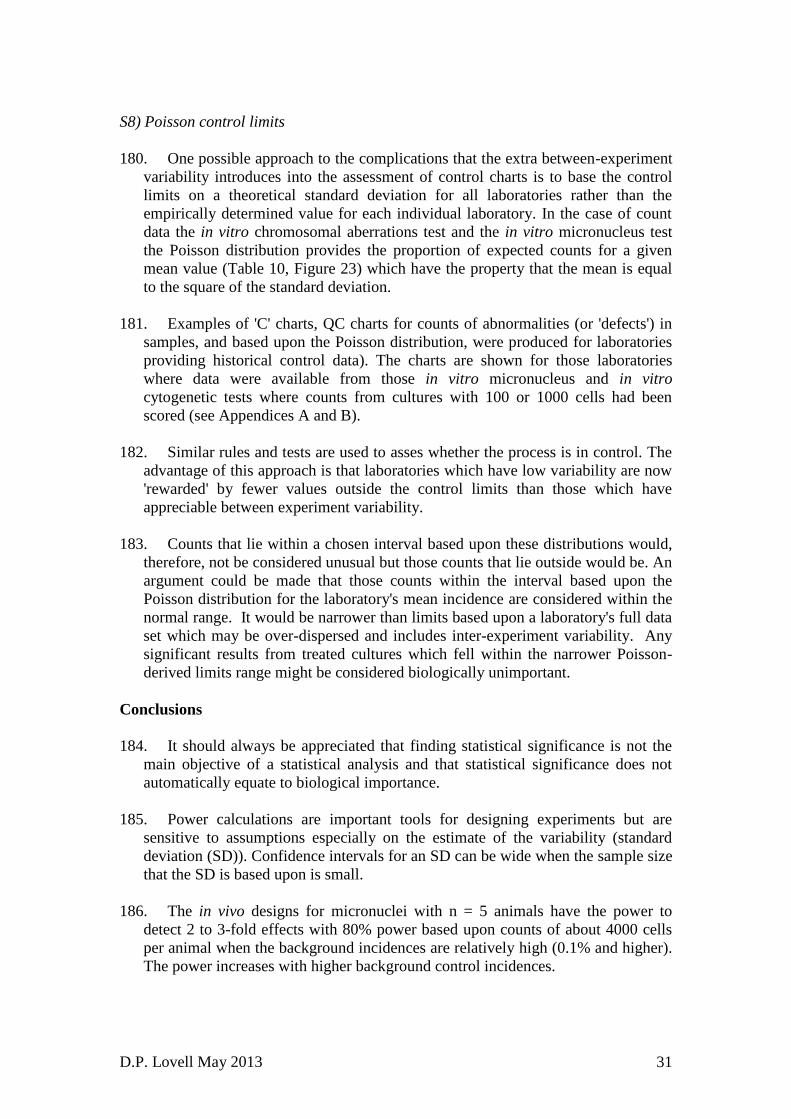
D.P. Lovell May 2013 31
S8) Poisson control limits
180. One possible approach to the complications that the extra between-experiment
variability introduces into the assessment of control charts is to base the control
limits on a theoretical standard deviation for all laboratories rather than the
empirically determined value for each individual laboratory. In the case of count
data the in vitro chromosomal aberrations test and the in vitro micronucleus test
the Poisson distribution provides the proportion of expected counts for a given
mean value (Table 10, Figure 23) which have the property that the mean is equal
to the square of the standard deviation.
181. Examples of 'C' charts, QC charts for counts of abnormalities (or 'defects') in
samples, and based upon the Poisson distribution, were produced for laboratories
providing historical control data). The charts are shown for those laboratories
where data were available from those in vitro micronucleus and in vitro
cytogenetic tests where counts from cultures with 100 or 1000 cells had been
scored (see Appendices A and B).
182. Similar rules and tests are used to asses whether the process is in control. The
advantage of this approach is that laboratories which have low variability are now
'rewarded' by fewer values outside the control limits than those which have
appreciable between experiment variability.
183. Counts that lie within a chosen interval based upon these distributions would,
therefore, not be considered unusual but those counts that lie outside would be. An
argument could be made that those counts within the interval based upon the
Poisson distribution for the laboratory's mean incidence are considered within the
normal range. It would be narrower than limits based upon a laboratory's full data
set which may be over-dispersed and includes inter-experiment variability. Any
significant results from treated cultures which fell within the narrower Poisson-
derived limits range might be considered biologically unimportant.
Conclusions
184. It should always be appreciated that finding statistical significance is not the
main objective of a statistical analysis and that statistical significance does not
automatically equate to biological importance.
185. Power calculations are important tools for designing experiments but are
sensitive to assumptions especially on the estimate of the variability (standard
deviation (SD)). Confidence intervals for an SD can be wide when the sample size
that the SD is based upon is small.
186. The in vivo designs for micronuclei with n = 5 animals have the power to
detect 2 to 3-fold effects with 80% power based upon counts of about 4000 cells
per animal when the background incidences are relatively high (0.1% and higher).
The power increases with higher background control incidences.

D.P. Lovell May 2013 32
187. Larger sample sizes, either as more animals and/or many more cells, would be
needed to have sufficient power to detect a 2-3 fold incidence when the
background incidence is lower (i.e. <0.05%).
188. Power calculations derived by Kissling et al and Health Canada are broadly in
agreement. Differences between them may derive from the use of different
statistical tests and methods for incorporating inter-individual variability in the
simulations. (They also broadly agree with those derived by other workers in the
field.)
189. In the case of the in vitro tests, power calculations and simulations provide
similar conclusions that sample sizes (cells or cultures/animals) would need to be
increased appreciably to detect doubling. The power to detect doubling/fold
increase is low especially when the background level is low (i.e. 0.5% for
chromosomal aberrations or 0.05% for micronuclei.
190. The power of the in vitro chromosome aberration test to detect a fold increase
is particularly low. The number of cells needed to detect a fold increase would
need to be increased appreciably to detect doubling. The actual numbers depend
upon the background incidence.
191. Replicate (duplicate) negative control samples are advisable on theoretical
grounds (at least until it can be shown that there is evidence of no appreciable
replicate variability). Increasing the number of replicate cultures increases the
statistical 'credibility' of the result but needs to be weighted against any increased
complexity in the conduct of the study introducing extra variability.
192. Increasing the number of cells in the negative control cultures (from say 200 to
400) provides a small increase in power and a better estimate of the negative
control incidence. This provides more robust comparisons when multiple
concentrations are tested but increases the complexity of the study.
193. If duplicate negative control cultures are homogeneous then the data can be
pooled across cultures. This is a pragmatic approach to increasing the power a
little but it is important to appreciate that this may affect (slightly) the error rates
associated with the analysis. If duplicate cultures are significantly different from
one another this probably introduces quality control issues and raises the question
as to whether the experiment meets acceptance criteria.
194. Trend tests with a smaller number of concentration levels have slightly higher
power based upon the Nam equation approach than those with more levels. Power
is quite high for detecting linear trends but will be reduced and the interpretation
more complex if the response is not linear. The use of 6 concentration levels
instead of 3 concentration levels may reduce the power of the linear trend test
slightly but may give more information on the shape of the concentration-response
relationship. More concentration levels should be used when there is specific
interest in the concentration-response.

D.P. Lovell May 2013 33
195. Trends tests are statistically more powerful for detecting linear concentration-
response relationships than pair-wise comparisons. Statistical tests are available
for identifying concentration-response relationships which differ from linear.
196. Use of multiple comparison methods is controversial especially when the
number of concentration groups differs. The Cochran-Arbitrage test for linear
trend is a 'powerful' test while Fisher's exact tests with a multiple comparison
correction for pairs of results are 'conservative'. It is important that the specific test
used to produce a P-value and declare a result as statistically significant or not is
explicitly stated.
197. The in vitro chromosomal aberration data showed no obvious differences
between the different cell lines or different S9 mix conditions. The range of mean
values (% aberrations) combined over all conditions for each of the cell lines was
0.20 to 1.07 for HPBL cells, 0.53 to 0.81 for CHO cells and 0.09 to 1.06 (with an
outlying laboratory with a mean of 2.16%). The lowest value for an individual
culture was 0%, of which there were many examples and the highest value was
6%.
198. The micronucleus data showed appreciable intra- and inter-laboratory
variability making it difficult identify a range that could be considered a 'normal
range' across all laboratories. The range of mean values (% micronuclei)
combined over all conditions for each of the cell lines was 0.45 to 1.39 for HPBL
cells, 0.21 to 0.59 for L5178Y cells and 0.42 to 1.13 for TK6 cells. The lowest
value for an individual culture was 0%, of which there were many examples and
the highest value was 2.8% (28/1000).
199. In the chromosome aberration dataset values ≥5 or aberrant cells rarely
occurred in a 100 cell sample and, based upon the Poisson distribution, when the
laboratory negative control mean is between 0.5% and 2.5% values ≥4 aberrant
cells have low probability and so values between 0 and 4 could be considered to
fall into the normal range.
200. Poisson distributed data have the property that the mean is equal to the
variance. A square root transformation (or a logarithmic transformation) can be
used to allow the data to be analysed by standard statistical methods. More
sophisticated modelling methods are also suitable methods for analysis of the data.
201. The Poisson distribution approximates to a normal distribution when np ≥5
where n is the number of cells and the mean proportions of cells with aberrations
or micronuclei is p. Scoring sufficient cells from a culture to produce mean counts
of 5 should provide data which approximates to a normal distribution.
202. Zero counts can be avoided by counting enough cells which are Poisson
distributed to obtain a mean number of counts/culture of 5. If this is achieved on
average only 0.7% of cultures would have zero counts. To obtain np = 5 from
cultures with a mean of 1% chromosomal aberrations, 500 cells need to be scored;
for cultures with 0.1% micronucleated cells 5000 cells would need to be scored.

D.P. Lovell May 2013 34
203. While counting sufficient cells to produce means of approximately 5 is
convenient for avoiding zero counts and for obtaining approximately normally
distributed data this is not a prerequisite for statistical analysis as statistical
method are available for handling such situations.
204. Analyses using the concurrent control should be the primary analysis of the
experimental data to test for treatment-related effects. Historical control data may
help with the interpretation of the biological importance of the results. (Data to be
included in the formal analysis should be within acceptance criteria. These criteria
may need to be defined.)
205. Laboratories should provide historic negative control data using quality
control methods such as control charts to identify how variable their data are and
to show that the methodology is 'under control' in their laboratory. A process in
'control' "exhibits only random variation within the control limits”
206. It is important to ensure that experiments that 'fail' (i.e. do not meet acceptance
criteria) are also included in the historical control dataset.
207. Most methods for using the historical control data to help determine a positive
result and in the assessment of the biological importance of the results have some
limitations. The GEF (Global Equivalence Factor) approach used in the Mouse
Lymphoma Assay (MLA) test may have some potential.
208. Control limits based upon the between cultures (or between study) standard
deviations can be used to specify upper and lower control limits. Use of these
when there is appreciable between-laboratory variability can 'reward' laboratories
that have high variability.
209. The use of C-charts, developed for quality control purposes with control limits
based upon the Poisson distribution to set the UCL could provide an indication of
results that would not be considered unusual as a way of identifying 'a normal
range' for the historical control range as well as those which would indicate an
effect had occurred.

D.P. Lovell May 2013 35
References
Galloway, S., Holder, D.J. & Armstrong, M. J. (2012) Sensitivity and power of the
bone marrow micronucleus (MN) test related to background level and sample sizes.
Poster presented at the GTA meeting 2012
Haseman, J.K., Huff, J. & Boorman, G.A (1984) Use of historical control data in
carcinogenicity studies in rodents Toxicologic Pathology. 12 126-135.
Hayes, J., Doherty, A.T., Adkins, D.J., Oldman, K. & O’Donovan, M.R. (2009) The
rat bone marrow micronucleus test—study design and statistical power. Mutagenesis
24 419-424.
Hayashi, M., Dearfield, K., Kasper P., Lovell D. & Thybaud, V. (2011) Compilation
and use of genetic toxicity historical control data. Mutation Research 723 87-90.
Health Canada (2012) Discussion Document on Assay Sensitivity, Sample Size and
Statistical Power for the Erythrocyte Micronucleus Assay (TG 474) produced for the
OECD expert group meeting.
Kissling, G.E., Dertinger, S.D., Hayashi, M. & MacGregor, J.T. (2007) Sensitivity of
the erythrocyte micronucleus assay: dependence on number of cells scored and inter-
animal variability. Mutation Research 634 235–240.
Margolin B.H., Resnick, M.A., Rimpo, J.Y., Archer, P., Galloway, S.M., Bloom, A.D.
& Zeiger, E. (1986) Statistical analyses for in vitro cytogenetic assays using Chinese
hamster ovary cells. Environ Mutagen. 8 183-204.
Moore, M.M., Honma, M., Clements, J., Bolcsfoldi, G., Burlinson, B., Cifone, M.,
Clarke, J., Delongchamp, R., Durward, R., Fellows, M., Gollapudi, B., Hou, S.,
Jenkinson, P., Lloyd, M., Majeska, J., Myhr, B., O’Donovan, M., Omori, T., Riach,
C., San, R., Stankowski, L.F. Jr., Thakur, A.K., Van Goethem, F., Wakuri, S. &
Yoshimura, I. (2006). Mouse lymphoma thymidine kinase gene mutation assay:
follow-up meeting of the international workshop on genotoxicity testing, Aberdeen,
Scotland, 2003, assay acceptance criteria, positive controls, and data evaluation,
Environmental and Molecular Mutagenesis 47 1-5.
Nam JM. (1987) A simple approximation for calculating sample sizes for detecting
linear trend in proportions. Biometrics 43 701-705
Soper, K.A. & Galloway S.M. (1994). Replicate flasks are not necessary for in vitro
chromosome aberration assays in CHO cells. Mutation Research 312 139-149.
D.P. Lovell May 2013 36
Table 1 95% upper and lower confidence limits of estimates of Kissling et al's
(2007) (Table 3) standard deviations
Table 2 Fold changes detectable at 90% and 95% power for various negative
control incidence and numbers of cells counted as derived by Kissling et al and
Health Canada (group size =5)
Table 3 Results of simulations using Health Canada's R program to investigate
the effect of varying numbers of animals and cells. Results are the fold increases
detectable for 80% power at P=0.05 (for group sizes, n, = 4, 5 and 6)
% n 4 5 6
0.05 2000 3.8 3.5 3.3
4000 2.8 2.6 2.4
8000 2.2 2.0 1.9
20000 1.7 1.6 1.5
0.10 2000 2.7 2.6 2.4
4000 2.2 2.0 1.9
8000 1.8 1.7 1.6
20000 1.4 1.4 1.4
0.20 2000 2.2 2.0 1.9
4000 1.8 1.7 1.6
8000 1.5 1.5 1.4
20000 1.3 1.3 1.3
0.30 2000 1.9 1.8 1.7
4000 1.6 1.6 1.5
8000 1.4 1.4 1.3
20000 1.2 1.2 1.2

D.P. Lovell May 2013 37
Table 4 Power calculation using nQuery Advisor to identify fold changes
detected with 80% power using the means and SDs from Kissling et al paper
(and assuming number of cells per animal =∞ as in their Table 3 for sample sizes
of 4, 5 and 6)
Mean SD 4 5 6
0.10 & 0.045 1.90 1.78 1.69
0.05 & 0.02 1.80 1.69 1.62
0.20 & 0.70 1.70 1.60 1.54
0.20 & 0.59 1.59 1.51 1.46
0.30 & 0.92 1.62 1.53 1.48

D.P. Lovell May 2013 38
Table 5 Table of descriptive statistics of data from laboratories for in vitro cytogenetics tests
Lab ID Cell type Type
% abs Zeros Celle N Mean* St Dev Min Max P-value
CB HPBL Count 0.24 315 200 466 0.49 0.85 0 5 <0.001
CC HPBL Count 1.07 63 100 146 1.07 1.25 0 6 0.01
CD HPBL Count 0.78 107 100 208 0.78 0.99 0 5 0.003
CE HPBL Count 0.74 83 100 164 0.74 0.90 0 4 0.39
CN HPBL Count 1.02 7 200 41 2.05 1.41 0 5 0.69
CP HPBL Count 0.20 105 100 128 0.20 0.44 0 2 0.89
CS HPBL Count 0.21 60 100 76 0.21 0.41 0 1 ND
CU HPBL Count 0.60 36 200 120 1.21 1.11 0 5 0.97
CA CHO Count 0.53 116 200 255 1.07 1.35 0 6 <0.001
CF CHO Count 0.81 80 100 180 0.81 0.94 0 5 0.61
CG CHL/IU Count 0.13 134 100 150 0.13 0.39 0 2 0.043
CH CHL/IU Count 0.09 280 100 300 0.09 0.36 0 3 0.001
CI CHL/IU Count 0.40 131 100 200 0.40 0.59 0 2 0.45
CJ CHL/IU Count 0.78 163 100 424 0.78 0.74 0 3 <0.001
CK CHL/IU Count 0.27 37 100 48 0.27 0.54 0 2 0.59
CL CHL/IU Count 0.50 653 100 911 0.50 0.98 0 4 <0.001
CM CHL/IU Count 2.16 52 200 85 4.32 2.62 0 10 <0.001
CO CHL/IU Count 1.06 52 100 144 1.06 1.05 0 4 0.91
CQ CHL/IU Count 0.22 14 100 18 0.22 0.43 0 1 ND
CR CHL/IU Count 0.44 32 100 54 0.44 0.57 0 2 0.11
CT CHL/IU Count 0.22 190 100 236 0.22 0.48 0 2 0.33
N Number of independent cultures Note three other laboratories reported data that could be summarized
P- value P-value of goodness of fit test for fit to Poisson distribution CX CHO 2115 cultures with a mean of 1.41% with an SD of 0.91% * Mean of counts from 100 or 200 cells CX HPBL 68 cultures with a mean of 1.73% with an SD of 0.60%
CV HPBL 73 cultures with a mean of 1.12% with an SD of 1.07%
CW CHL/IU 238 cultures with a mean of 0.38% with an SD of 0.70%

D.P. Lovell May 2013 39
Table 6 Table of descriptive statistics of data from laboratories for in vitro micronucleus tests
Lab ID Cell type BC Cyto Type
%mnt Zeros Cells N Mean
* St Dev Min Max P value
MA HPBL Y NI Count 0.58 1 1000 171 5.81 3.13 0 21 0.003
MC HPBL N NI Count 0.45 2 1000 204 4.46 2.93 0 15 <0.001
MH HPBL N NI Count 1.39 0 2000 36 27.81 17.30 6 68 N/D
MJ HPBL N NI Count 0.17 10 1000 54 1.67 1.24 0 5 0.85
MK HPBL N NI Count 0.64 0 1000 68 6.38 3.12 1 14 0.017
MM2 HPBL N NI Non-integer 0.70 2000 28 13.96 4.84 7 26.4 N/D
MB L5178Y N N Count 0.21 21 1000 138 2.11 1.51 0 7 0.66
MD1 L5178Y N NI Count 0.54 2 1000 518 5.44 2.61 0 19 <0.001
ML2 L5178Y N NI Non-integer 0.28 ?1000 767 2.80 1.21 0 8 N/D
MM1 L5178Y N NI Non-integer 0.59 2000 126 11.79 4.24 4 21.8 N/D
MI CHL/IU N NI Count 0.35 0 1000 154 3.51 1.01 1 6 <0.001
MD2 TK6 N NI Count 1.13 1 1000 98 11.31 3.42 2 21 0.26
ME TK6 Y Y Count 0.42 0 1000 59 4.15 2.14 1 11 0.44
MF TK6 N Y Non-integer 0.71 1000 198 7.06 3.95 1 28 N/D
MG TK6 N NI Count 0.82 0 2000 36 16.47 3.61 9 26 N/D
ML1 TK6 N NI Non-integer 0.42 ?1000 166 4.25 1.64 0 8.3 N/D
N Number of independent cultures BC Specific comment about binucleated cells being scored (Y/N)
NI No information Cyto Specific comment on use of cytochalasin-B (Y/N/NI)
N/D Not done because data not suitable for test
?1000 Number of cells that summary statistic based on is not clear, presumed 1000 *
Mean count based upon 1000 or 2000 cells
P value P value of goodness of fit test for fit to Poisson distribution
D.P. Lovell May 2013 40
Table 7 Fold change that would be detected in a pair-wise test for different
control incidences and sample sizes in the in vitro micronucleus test
%
Cells 0.05 0.1 0.15 0.2 0.3 0.4 0.5
1000 15.1 8.7 6.6 5.4 4.3 3.7 3.3
2000 8.8 5.5 4.3 3.7 3.0 2.7 2.5
4000 5.5 3.7 3.0 2.7 2.3 2.1 2.0
5000 4.8 3.3 2.8 2.5 2.1 2.0 1.8
10000 3.3 2.5 2.1 2.0 1.8 1.6 1.6
Table 8 Power associated with the design for detecting a fold increase or
doubling over the negative control incidence in a pair-wise test for the in vitro
micronucleus test.
%
Cells 0.05 0.1 0.15 0.2 0.3 0.4 0.5
1000 0.11 0.14 0.17 0.20 0.26 0.31 0.36
2000 0.14 0.20 0.26 0.31 0.41 0.50 0.57
4000 0.20 0.31 0.41 0.50 0.64 0.75 0.83
5000 0.23 0.36 0.48 0.57 0.72 0.83 0.89
10000 0.36 0.57 0.72 0.83 0.94 0.98 0.99
Table 9 Confidence intervals for the expected value (parameter) of a Poisson
random variable.
(from: http://faculty.washington.edu/heagerty/Books/Biostatistics/TABLES/Poisson/index.html)

D.P. Lovell May 2013 41
Table 10 Proportions of counts of 0, 1, 2, 3 etc when each column here represents
the underlying mean of the population (i.e. 1, 2, 3), For example 37% of cultures
will have zero micronuclei and a further 37% will have one micronucleus when
the mean level is 1 per culture.
Mean N 1 2 3 4 5 6 7 8 9 10
0 0.37 0.14 0.05 0.02 0.01 0.00 0.00 0.00 0.00 0.00
1 0.37 0.27 0.15 0.07 0.03 0.01 0.01 0.00 0.00 0.00
2 0.18 0.27 0.22 0.15 0.08 0.04 0.02 0.01 0.00 0.00
3 0.06 0.18 0.22 0.20 0.14 0.09 0.05 0.03 0.01 0.01
4 0.02 0.09 0.17 0.20 0.18 0.13 0.09 0.06 0.03 0.02
5 0.00 0.04 0.10 0.16 0.18 0.16 0.13 0.09 0.06 0.04
6 0.00 0.01 0.05 0.10 0.15 0.16 0.15 0.12 0.09 0.06
7 0.00 0.00 0.02 0.06 0.10 0.14 0.15 0.14 0.12 0.09
8 0.00 0.00 0.01 0.03 0.07 0.10 0.13 0.14 0.13 0.11
9 0.00 0.00 0.00 0.01 0.04 0.07 0.10 0.12 0.13 0.13
10 0.00 0.00 0.00 0.01 0.02 0.04 0.07 0.10 0.12 0.13

D.P. Lovell May 2013 42
Table 11 The percentage of cultures with from 0 to 15 aberrant or micronucleated cells in samples of size n cells when the 'true' mean
number in cultures range from 0.5 to 5.
Number of cells with an aberration or a micronucleus in culture
Mean 0 1 2 3 4 5 6 7 8 9 10 11 12 13 14 15
0.5 60.7 30.3 7.6 1.3 0.2 0.0 0.0 0.0 0.0 0.0 0.0 0.0 0.0 0.0 0.0 0.0
1.0 36.8 36.8 18.4 6.1 1.5 0.3 0.1 0.0 0.0 0.0 0.0 0.0 0.0 0.0 0.0 0.0
1.5 22.3 33.5 25.1 12.6 4.7 1.4 0.4 0.1 0.0 0.0 0.0 0.0 0.0 0.0 0.0 0.0
2.0 13.5 27.1 27.1 18.0 9.0 3.6 1.2 0.3 0.1 0.0 0.0 0.0 0.0 0.0 0.0 0.0
2.5 8.2 20.5 25.7 21.4 13.4 6.7 2.8 1.0 0.3 0.1 0.0 0.0 0.0 0.0 0.0 0.0
3.0 5.0 14.9 22.4 22.4 16.8 10.1 5.0 2.2 0.8 0.3 0.1 0.0 0.0 0.0 0.0 0.0
3.5 3.0 10.6 18.5 21.6 18.9 13.2 7.7 3.9 1.7 0.7 0.2 0.1 0.0 0.0 0.0 0.0
4.0 1.8 7.3 14.7 19.5 19.5 15.6 10.4 6.0 3.0 1.3 0.5 0.2 0.1 0.0 0.0 0.0
4.5 1.1 5.0 11.3 16.9 19.0 17.1 12.8 8.2 4.6 2.3 1.0 0.4 0.2 0.1 0.0 0.0
5.0 0.7 3.4 8.4 14.0 17.6 17.6 14.6 10.4 6.5 3.6 1.8 0.8 0.3 0.1 0.1 0.0
Mean is count per culture. Mean of 5 is an incidence of 1% if 500 cells are scored or 5% if 100 cells are scored. (Assumes Poisson distributions. If an individual laboratory
scores are 'over-dispersed' then the number of zeros may be increased for a given mean.)
Poisson distribution approximates to a normal distribution when np >5
Table can be used to identify the number of cells to score to have a low probability of encountering a zero count. For instance, to have <1% of cultures having zero scores
when the mean is 2.5/100 cells then 200 cells/culture would need to be scored.
For chromosomal aberrations
% p np equivalent to:
1 0.01 1 2/50 1/100 0.5/200 0.2/500
5 0.05 5 10/50 5/100 2.5/200 1/500
For micronuclei
% p np equivalent to:
0.1 0.001 1 2/500 1/1000 0.5/2000 0.2/5000
0.5 0.005 5 10/500 5/1000 2.5/2000 1/5000

D.P. Lovell May 2013 43
Figure 1 Histogram of mean % incidence of chromosomal aberration in 65
combinations of cell types, S9 fractions and treatment times
2.52.01.51.00.50.0
20
15
10
5
0
Mean
Fre
qu
en
cy
Histogram of Mean

D.P. Lovell May 2013 44
Figure 2. Means and 95% confidence intervals for the incidence of
chromosomal aberrations in 65 sets of samples from 19 laboratories. Colour
codes: Black, HPBL; Red, CHO; Green, CHL/IU. (Means are % cells with
chromosomal aberrations) (The size of the confidence interval depends in part
on the sample size: very narrow intervals are based upon large samples; wide
intervals on small sample sizes)

D.P. Lovell May 2013 45
Figure 3. Means and standard deviations for the incidence of chromosomal
aberrations in 65 sets of samples from 19 laboratories. Colour codes: Black, –S9
fraction; Red, +S9 fraction; Green, samples combined over S9 conditions
(Means are % cells with chromosomal aberrations)

D.P. Lovell May 2013 46
Figure 4 In vitro chromosome aberration test: Distribution of individual counts
of numbers of chromosomal aberrations from (where possible) individual
cultures for each laboratory, HPBL cells (n=100)
6543210
6543210
100
75
50
25
0
6543210
100
75
50
25
0
CC
Fre
qu
en
cy
CD CE
CP CS
Histogram of HPBL (100 cells)
CC Counts from % Cabs based upon 100 cells
CD Counts based upon 100 cells
CE Counts based upon approx 100 cells
CP Counts based upon 100 cells except some on 50 and 200 which were mainly
negative
CS Counts based upon 100 cells for single culture

D.P. Lovell May 2013 47
Figure 5 In vitro chromosome aberration test: Distribution of individual counts
of numbers of chromosomal aberrations from (where possible) individual
cultures for each laboratory, HPBL cells (n=100) and HPBL cell (n=200)
543210
300
200
100
0
543210
300
200
100
0
CB
Fre
qu
en
cy
CN
CU
Histogram of HPBL (200 cells)
CB % abs based upon 200 cells x2 to create counts
CN % abs based upon 200 cells x2 to create counts
CU % abs based upon 200 cells x2 to create counts

D.P. Lovell May 2013 48
Figure 6 In vitro chromosome aberration test: Distribution of individual counts
of numbers of chromosomal aberrations from (where possible) individual
cultures for each laboratory, CHO cells
6543210
120
100
80
60
40
20
0
6543210
CA
Fre
qu
en
cy
CF
Histogram of CHO (CA 200 cells, CF 100 cells)
CA % abs based upon 200 cells x 2 to create counts
CF Counts based upon approx 100 cells

D.P. Lovell May 2013 49
Figure 7 In vitro chromosome aberration test: Distribution of individual counts
of numbers of chromosomal aberrations from (where possible) individual
cultures for each laboratory, CHL/IU cells
43210
600
450
300
150
0
43210
600
450
300
150
043210
CG
Fre
qu
en
cy
CH CI
CJ CK CL
Histogram of CHL/IU (100 cells)
CG Counts based upon approx 100 cells
CH Counts based upon approx 100 cells
CI Counts based upon approx 100 cells
CJ Counts based upon approx 100 cells
CK Counts based upon approx 100 cells
CL Counts based upon 100 cells except some on 50 which were mainly zero

D.P. Lovell May 2013 50
Figure 8 In vitro chromosome aberration test: Distribution of individual counts
of numbers of chromosomal aberrations from (where possible) individual
cultures for each laboratory, CHL/IU cells
1086420
1086420
200
150
100
50
0
1086420
200
150
100
50
0
CO
Fre
qu
en
cy
CQ CR
CT CM
Histogram of CHL/IU (100 cells, except CM 200 cells)
CO Counts based upon 100 cells
CQ Counts based upon 100 cells
CR Counts based upon 100 cells for single culture
CT Counts based upon 100 cells for single culture
CM Counts based upon 200 cells summed over 2 cultures

D.P. Lovell May 2013 51
Figure 9 Power curves for pair-wise test for different number of cell (50 to 500)
with an incidence of 0.5% (proportion p of 0.005) chromosome aberrations in the
negative control culture
0.250.200.150.100.05
1.0
0.8
0.6
0.4
0.2
0.0
Comparison p
Po
we
r
A lpha 0.05
Baseline p 0.005
A lternativ e >
A ssumptions
50
100
200
500
Size
Sample
Power Curve for Two Proportions
Figure 10 Power curves for pair-wise test for different number of cell (50 to 500)
with an incidence of 1.0% (proportion p of 0.01) chromosome aberrations in the
negative control culture
0.250.200.150.100.05
1.0
0.8
0.6
0.4
0.2
0.0
Comparison p
Po
we
r
A lpha 0.05
Baseline p 0.01
A lternativ e >
A ssumptions
50
100
200
500
Size
Sample
Power Curve for Two Proportions
D.P. Lovell May 2013 52
Figure 11 Power curves for pair-wise test for different number of cell (50 to 500)
with an incidence of 2.0% (proportion p of 0.02) chromosome aberrations in the
negative control culture
0.250.200.150.100.05
1.0
0.8
0.6
0.4
0.2
0.0
Comparison p
Po
we
r
A lpha 0.05
Baseline p 0.02
A lternativ e >
A ssumptions
50
100
200
500
Size
Sample
Power Curve for Two Proportions

D.P. Lovell May 2013 53
Figure 12 Histogram of mean % incidence of micronucleated cells in 53
combinations of cell types, S9 fractions and treatment times from 13 laboratories
1.51.20.90.60.3
18
16
14
12
10
8
6
4
2
0
Mean
Fre
qu
en
cy
Histogram of Mean

D.P. Lovell May 2013 54
Figure 13 Means and 95% confidence intervals for the incidence of micronuclei
in 53 sets of samples from 13 laboratories. Colour codes: Black, L5178Y; Red,
HPBL; Green, TK6; Blue, CHL/IU (Means are cells with micronuclei/1000 cells)
(The size of the confidence interval depends in part on the sample size: very
narrow intervals are based upon large samples; wide intervals on small sample
sizes)

D.P. Lovell May 2013 55
Figure 14 Means and standard deviations for the incidence of micronuclei in 53
sets of samples from 13 laboratories. Colour codes: Black, –S9 fraction; Red, +S9
fraction; Green, samples combined over S9 conditions (Means are cells with
micronuclei/1000 cells)

D.P. Lovell May 2013 56
Figure 15 In vitro micronucleus test: Distribution of individual counts of
numbers of micronuclei from (where possible) individual cultures for each
laboratory: HPBL cells
706050403020100
120
90
60
30
0
706050403020100
120
90
60
30
0706050403020100
MA
Fre
qu
en
cy
MC MH
MJ MK MM2
Histogram of in vitromicornuclei: HPBL
MA count from 1000 cells
MC count from 1000 cells
MH count based upon 2000 cells (data converted from %MN to count based upon
2000 cells)
MJ count from 1000 cells
MK count from 1000 and some 500 cells
MM2 count based upon 2000 cells (data converted from %MN to count based upon
2000 cells)

D.P. Lovell May 2013 57
Figure 16 In vitro micronucleus test: Distribution of individual counts of
numbers of micronuclei from (where possible) individual cultures for each
laboratory: L5178Y cells
211815129630
240
180
120
60
0
211815129630
240
180
120
60
0
MB
Fre
qu
en
cy
MD1
ML2 MM1
Histogram of in vitro micronuclei: L5178Y cells
.
MB count from 1000 cells
MD1 count from 1000 cells (slight adjustments)
ML2 %MN x 10 (not possible to recreate counts)
MM1 count based upon 2000 cells (data converted from %MN to count based upon
2000 cells)

D.P. Lovell May 2013 58
Figure 17 In vitro micronucleus test: Distribution of individual counts of
numbers of micronuclei from (where possible) individual cultures for each
laboratory: CHL/IU and TK6 cells
2824201612840
100
75
50
25
0
2824201612840
100
75
50
25
02824201612840
MI
Fre
qu
en
cy
MD2 ME
MF MG ML1
Histogram of in vitro micronuclei: CHL/IU and TK cells
CHL/IU cells
MI %MN x 10 from 1000 cells
TK6 cells
MD2 count from 1000 cells (slight adjustments)
ME count from 1000 cells
MF 'approximate' counts from 1000 cells
MG based upon 2000 cells (data converted from %MN to count based upon 2000
cells)
ML1 %MN x10 (not possible to recreate counts)

D.P. Lovell May 2013 59
Figure 18 Power curves for pair-wise test for different numbers of cells (1000 to
10000) with an incidence of 0.05% (proportion p of 0.0005 or 0.5/1000)
micronuclei in the negative control culture
0.0160.0140.0120.0100.0080.0060.0040.002
1.0
0.8
0.6
0.4
0.2
0.0
Comparison p
Po
we
r
A lpha 0.05
Baseline p 0.0005
A lternativ e >
A ssumptions
1000
2000
4000
5000
10000
Size
Sample
Power Curve for Two Proportions
Figure 19 Power curves for pair-wise test for different numbers of cells (1000 to
10000) with an incidence of 0.1% (proportion p of 0.001 or 1/1000) micronuclei
in the negative control culture
0.0180.0160.0140.0120.0100.0080.0060.0040.002
1.0
0.8
0.6
0.4
0.2
0.0
Comparison p
Po
we
r
A lpha 0.05
Baseline p 0.001
A lternativ e >
A ssumptions
1000
2000
4000
5000
10000
Size
Sample
Power Curve for Two Proportions

D.P. Lovell May 2013 60
Figure 20 Power curves for pair-wise test for different numbers of cells (1000 to
10000) with an incidence of 0.2% (proportion p of 0.002 or 2/1000) micronuclei
in the negative control culture
0.0200.0150.0100.005
1.0
0.8
0.6
0.4
0.2
0.0
Comparison p
Po
we
r
A lpha 0.05
Baseline p 0.002
A lternativ e >
A ssumptions
1000
2000
4000
5000
10000
Size
Sample
Power Curve for Two Proportions
Figure 21 Power curves for pair-wise test for different numbers of cells (1000 to
10000) with an incidence of 0.5% (proportion p of 0.005 or 5/1000) micronuclei
in the negative control culture
0.0250.0200.0150.0100.005
1.0
0.8
0.6
0.4
0.2
0.0
Comparison p
Po
we
r
A lpha 0.05
Baseline p 0.005
A lternativ e >
A ssumptions
1000
2000
4000
5000
10000
Size
Sample
Power Curve for Two Proportions

D.P. Lovell May 2013 61
Figure 22 Plot of the percentage of zero counts for Poisson distributed data with
increasing population means
876543210
60
50
40
30
20
10
0
Mean
% z
ero
s
Plot of % zeros vs Mean for Poisson distributed data

D.P. Lovell May 2013 62
Figure 23 Poisson distribution for mean counts (N) from 1 to 10. Figure shows a
graphical representation of the data in Table 10.

D.P. Lovell May 2013 63
Figure 24 An illustration of how the Poisson distributions approximates to a
normal distribution as the mean count (N) increases from 1 to 25.

D.P. Lovell May 2013 64
Figure 25 Counts beyond the upper 5% (0.05) of the distribution (in red) for
different means based upon Poisson distributions with population means from
0.5 to 5.0
0.60
0.45
0.30
0.15
0.00
X
Pro
ba
bil
ity
3
0.01439
0
0.4
0.3
0.2
0.1
0.0
X
Pro
ba
bil
ity
4
0.01899
0
0.3
0.2
0.1
0.0
X
Pro
ba
bil
ity
5
0.01858
0
0.3
0.2
0.1
0.0
X
Pro
ba
bil
ity
6
0.01656
0
Distribution Plot
Poisson, Mean=0.5
Distribution Plot
Poisson, Mean=1
Distribution Plot
Poisson, Mean=1.5
Distribution Plot
Poisson, Mean=2
0.24
0.18
0.12
0.06
0.00
X
Pro
ba
bil
ity
6
0.04202
0
0.20
0.15
0.10
0.05
0.00
X
Pro
ba
bil
ity
7
0.03351
0
0.20
0.15
0.10
0.05
0.00
X
Pro
ba
bil
ity
9
0.02136
0
0.20
0.15
0.10
0.05
0.00
X
Pro
ba
bil
ity
10
0.03183
0
Distribution Plot
Poisson, Mean=2.5
Distribution Plot
Poisson, Mean=3
Distribution Plot
Poisson, Mean=4
Distribution Plot
Poisson, Mean=5

D.P. Lovell May 2013 65
Figure 26 In vitro chromosomal aberration test: combining counts of HPBL and
CHL/IU across laboratories (100 cells)
6543210
1600
1400
1200
1000
800
600
400
200
0
Data
Fre
qu
en
cy
CHL/IU comb
HPBL comb
Variable
Histogram of CHL/IU comb, HPBL comb
6543210
1600
1400
1200
1000
800
600
400
200
0
6543210
CHL/IU comb
Fre
qu
en
cy
HPBL comb
Histogram of CHL/IU comb, HPBL comb
Poisson mean for CHL/IU comb = 0.485 Chi-sq (3df) 440.9 P<0.001
Poisson mean for HPBL comb = 0.665 Chi-Sq(3df) 44.4 P<0.001
(Mean and Standard deviation can be used to calculate GEF)
Variable N Mean StDev Min Max GEF
CHL/IU comb 2373 0.48 0.83 0 4 1.31
HPBL comb 722 0.66 0.96 0 6 1.62

D.P. Lovell May 2013 66
Appendix 1: Quality control C charts of chromosomal aberration counts across
all cultures from laboratories where data can be expressed as counts.
The upper and lower control limits are based upon 2 and 3 SD based upon the Poisson
distribution.
The red points on graphs represent cases 'flagged' as outside controls based upon rules
1-4 defined as:
1) 1 point more than 3 standard deviations from the centre line
2) 9 points in a row on same side of centre line
3) 6 points in a row, all increasing or all decreasing
4) 14 points in a row, alternating up and down

D.P. Lovell May 2013 67
2512262011761511261017651261
6
5
4
3
2
1
0
Sample
Sam
ple
Co
un
t
_C=1.067
+3SL=4.165
-3SL=0
+2SL=3.132
-2SL=0
11
1
1
22
2
22
2
22
1
2
22
1
22
1
11
C Chart of CA
42437733028323618914295481
5
4
3
2
1
0
Sample
Sam
ple
Co
un
t
_C=0.485
+3SL=2.574
-3SL=0
+2SL=1.878
-2SL=0
1111
2
1111
22
11
222222
1
1
1
1
1
22222222
1
111
2
11
1
1
C Chart of CB

D.P. Lovell May 2013 68
1361211069176614631161
6
5
4
3
2
1
0
Sample
Sam
ple
Co
un
t
_C=1.068
+3SL=4.170
-3SL=0
+2SL=3.136
-2SL=0
1
1
1
2
2
22
C Chart of CC
190169148127106856443221
5
4
3
2
1
0
Sample
Sam
ple
Co
un
t
_C=0.779
+3SL=3.426
-3SL=0
+2SL=2.544
-2SL=0
1
C Chart of CD

D.P. Lovell May 2013 69
1611451291139781654933171
4
3
2
1
0
Sample
Sam
ple
Co
un
t
_C=0.738
+3SL=3.315
-3SL=0
+2SL=2.456
-2SL=0
1
2
C Chart of CE
16314512710991735537191
5
4
3
2
1
0
Sample
Sam
ple
Co
un
t
_C=0.811
+3SL=3.513
-3SL=0
+2SL=2.612
-2SL=0
11
C Chart of CF

D.P. Lovell May 2013 70
1361211069176614631161
2.0
1.5
1.0
0.5
0.0
Sample
Sam
ple
Co
un
t
_C=0.127
+3SL=1.194
-3SL=0
+2SL=0.838
-2SL=0222222222222
1
2222222222222222222222
11
222222222222
C Chart of CG
2712412111811511219161311
3.0
2.5
2.0
1.5
1.0
0.5
0.0
Sample
Sam
ple
Co
un
t
_C=0.087
+3SL=0.970
-3SL=0
+2SL=0.675
-2SL=02222222
1
2
11
22222222
1
1
222222
1
22
1
22222
1
1
2222222222222222222222222
1
2222
111
22
1
2222222222222222
11
22222222222
11
222222222222222222222222222222222222222222222
1
2222222
1
C Chart of CH

D.P. Lovell May 2013 71
181161141121101816141211
2.5
2.0
1.5
1.0
0.5
0.0
Sample
Sam
ple
Co
un
t
_C=0.4
+3SL=2.297
-3SL=0
+2SL=1.665
-2SL=02222222
C Chart of CI
42137933729525321116912785431
3.5
3.0
2.5
2.0
1.5
1.0
0.5
0.0
Sample
Sam
ple
Co
un
t
_C=0.783
+3SL=3.438
-3SL=0
+2SL=2.553
-2SL=0
2222
2
C Chart of CJ

D.P. Lovell May 2013 72
464136312621161161
2.0
1.5
1.0
0.5
0.0
Sample
Sam
ple
Co
un
t
_C=0.271
+3SL=1.832
-3SL=0
+2SL=1.312
-2SL=02
11
C Chart of CK
911820729638547456365274183921
4
3
2
1
0
Sample
Sam
ple
Co
un
t
_C=0.497
+3SL=2.613
-3SL=0
+2SL=1.908
-2SL=0
111111
22
2
222
2
2
2
22
2
1
111111
22
1
1
1
2222
11111
222
11
11
22222222222222222222222222222222
1
22222222
1
2222
1
222222222222222222222222222222222222222222222222222
1
2
1
222222
1
22222
111
111
111
1
22222222
1
1
111
11
1
2
1
1111
11
C Chart of CL

D.P. Lovell May 2013 73
81736557494133251791
12
10
8
6
4
2
0
Sample
Sam
ple
Co
un
t
_C=4.32
+3SL=10.55
-3SL=0
+2SL=8.47
-2SL=0.16
C Chart of CM
4137332925211713951
7
6
5
4
3
2
1
0
Sample
Sam
ple
Co
un
t
_C=2.049
+3SL=6.343
-3SL=0
+2SL=4.911
-2SL=0
C Chart of CN

D.P. Lovell May 2013 74
141127113998571574329151
4
3
2
1
0
Sample
Sam
ple
Co
un
t
_C=1.063
+3SL=4.155
-3SL=0
+2SL=3.124
-2SL=022222
2222
2
2222
22
2
C Chart of CO
118105927966534027141
2.0
1.5
1.0
0.5
0.0
Sample
Sam
ple
Co
un
t
_C=0.195
+3SL=1.521
-3SL=0
+2SL=1.079
-2SL=0
11
222222222222222222
C Chart of CP

D.P. Lovell May 2013 75
1715131197531
1.8
1.6
1.4
1.2
1.0
0.8
0.6
0.4
0.2
0.0
Sample
Sam
ple
Co
un
t
_C=0.222
+3SL=1.636
-3SL=0
+2SL=1.165
-2SL=02
C Chart of CQ
51464136312621161161
2.5
2.0
1.5
1.0
0.5
0.0
Sample
Sam
ple
Co
un
t
_C=0.444
+3SL=2.444
-3SL=0
+2SL=1.778
-2SL=0
C Chart of CR

D.P. Lovell May 2013 76
736557494133251791
1.6
1.4
1.2
1.0
0.8
0.6
0.4
0.2
0.0
Sample
Sam
ple
Co
un
t
_C=0.211
+3SL=1.587
-3SL=0
+2SL=1.128
-2SL=022222
C Chart of CS
10997857361493725131
5
4
3
2
1
0
Sample
Sam
ple
Co
un
t
_C=1.208
UCL=4.506
LCL=0
1
C Chart of CU

D.P. Lovell May 2013 77
Appendix 2: Quality control 'C' charts of micronuclei counts across all cultures
from laboratories where data can be expressed as counts.
The upper and lower control limits are based upon 2 and 3 SD based upon the Poisson
distribution.
The red points on graphs represent cases 'flagged' as outside control based upon rules
1-4 defined as:
1) 1 point more than 3 standard deviations from the centre line
2) 9 points in a row on same side of centre line
3) 6 points in a row, all increasing or all decreasing
4) 14 points in a row, alternating up and down

D.P. Lovell May 2013 78
17115413712010386695235181
20
15
10
5
0
Sample
Sam
ple
Co
un
t
_C=5.81
+3SL=13.04
-3SL=0
+2SL=10.63
-2SL=0.99
1
2
22
1
1
C Chart of MA
127113998571574329151
7
6
5
4
3
2
1
0
Sample
Sam
ple
Co
un
t
_C=2.109
+3SL=6.465
-3SL=0
+2SL=5.013
-2SL=0
2
2
2
1
2
2
2
C Chart of MB

D.P. Lovell May 2013 79
201181161141121101816141211
16
14
12
10
8
6
4
2
0
Sample
Sam
ple
Co
un
t
_C=4.46
+3SL=10.80
-3SL=0
+2SL=8.68
-2SL=0.24
1
1
2
222
1
1
22222
2
1
1
1
1
1
2
22
2
1
1
C Chart of MC
469417365313261209157105531
20
15
10
5
0
Sample
Sam
ple
Co
un
t
_C=5.44
+3SL=12.44
-3SL=0
+2SL=10.11
-2SL=0.782
1
1
1
1
2
2
1
1
1
1
1
1
C Chart of MD1

D.P. Lovell May 2013 80
9181716151413121111
20
15
10
5
0
Sample
Sam
ple
Co
un
t
_C=11.31
+3SL=21.39
-3SL=1.22
+2SL=18.03
-2SL=4.58
2
C Chart of MD2
554943373125191371
12
10
8
6
4
2
0
Sample
Sam
ple
Co
un
t
_C=4.15
+3SL=10.27
-3SL=0
+2SL=8.23
-2SL=0.08
1
C Chart of ME

D.P. Lovell May 2013 81
332925211713951
30
25
20
15
10
5
Sample
Sam
ple
Co
un
t
_C=16.47
+3SL=28.65
-3SL=4.30
+2SL=24.59
-2SL=8.36
C Chart of MG
1511361211069176614631161
9
8
7
6
5
4
3
2
1
0
Sample
Sam
ple
Co
un
t
_C=3.51
+3SL=9.14
-3SL=0
+2SL=7.26
-2SL=0
C Chart of MI

D.P. Lovell May 2013 82
51464136312621161161
6
5
4
3
2
1
0
Sample
Sam
ple
Co
un
t
_C=1.667
+3SL=5.540
-3SL=0
+2SL=4.249
-2SL=0
C Chart of MJ
645750433629221581
14
12
10
8
6
4
2
0
Sample
Sam
ple
Co
un
t
_C=6.38
+3SL=13.96
-3SL=0
+2SL=11.44
-2SL=1.33
2
2
1
2
2
222
2
22
C Chart of MK
Recommended