Statistics for Business and Economics
Random Variables & Probability Distributions
Learning Objectives
1. Distinguish Between the Two Types of Random Variables
2. Describe Discrete Probability Distributions
3. Describe the Binomial and Poisson Distributions
4. Describe the Uniform and Normal Distributions
Learning Objectives (continued)
5. Approximate the Binomial Distribution Using the Normal Distribution
6. Explain Sampling Distributions
7. Solve Probability Problems Involving Sampling Distributions
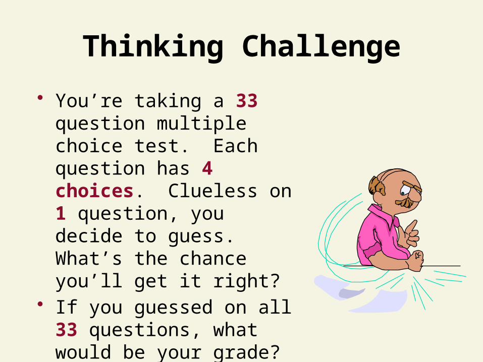
Thinking Challenge
• You’re taking a 33 question multiple choice test. Each question has 4 choices. Clueless on 1 question, you decide to guess. What’s the chance you’ll get it right?
• If you guessed on all 33 questions, what would be your grade? Would you pass?
Types of Random Variables
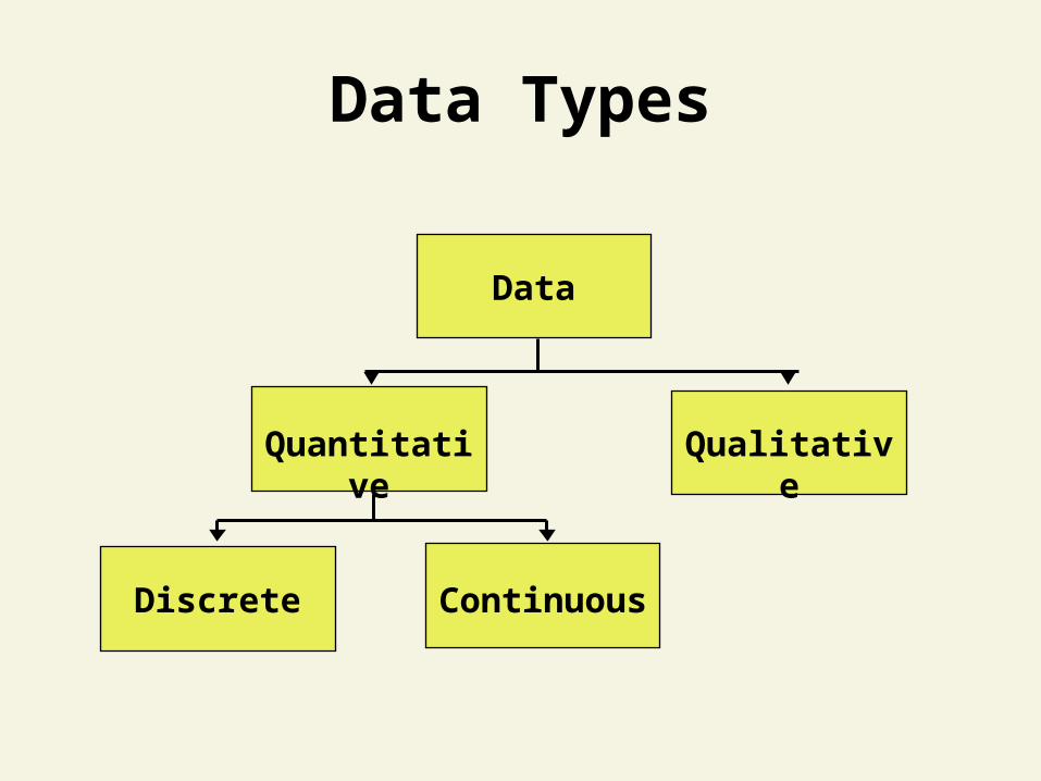
Data Types
Data
Quantitative Qualitative
ContinuousDiscrete
Discrete Random Variables
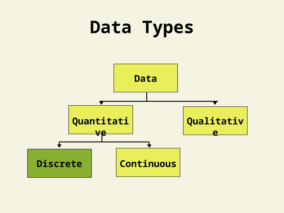
Data Types
Data
Quantitative Qualitative
ContinuousDiscrete
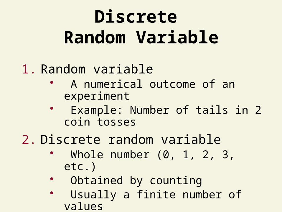
Discrete Random Variable
1. Random variable• A numerical outcome of an experiment• Example: Number of tails in 2 coin tosses
2. Discrete random variable • Whole number (0, 1, 2, 3, etc.)• Obtained by counting• Usually a finite number of values
— Poisson random variable is exception ()

Discrete Random Variable Examples
Experiment RandomVariable
PossibleValues
Count Cars at TollBetween 11:00 & 1:00
# CarsArriving
0, 1, 2, ..., ∞
Make 100 Sales Calls # Sales 0, 1, 2, ..., 100
Inspect 70 Radios # Defective 0, 1, 2, ..., 70
Answer 33 Questions # Correct 0, 1, 2, ..., 33
Continuous Random Variables

Data Types
Data
Quantitative Qualitative
ContinuousDiscrete
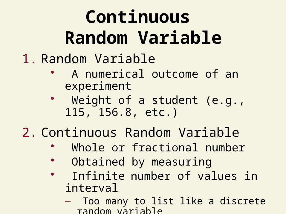
Continuous Random Variable
1. Random Variable• A numerical outcome of an experiment• Weight of a student (e.g., 115, 156.8, etc.)
2. Continuous Random Variable • Whole or fractional number• Obtained by measuring• Infinite number of values in interval
— Too many to list like a discrete random variable
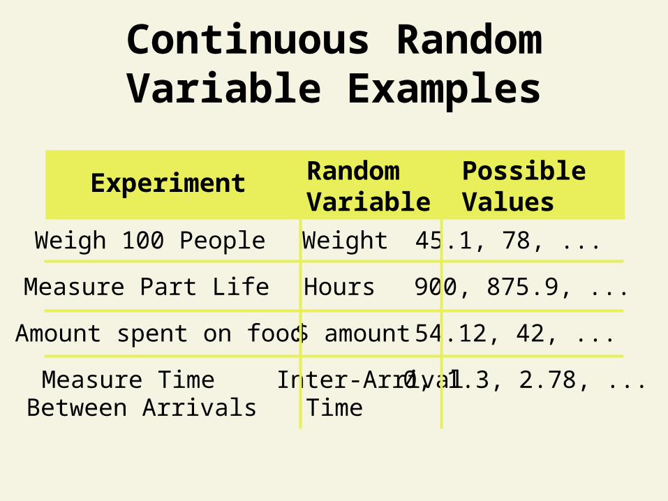
Continuous Random Variable Examples
Measure TimeBetween Arrivals
Inter-ArrivalTime
0, 1.3, 2.78, ...
Experiment RandomVariable
PossibleValues
Weigh 100 People Weight 45.1, 78, ...
Measure Part Life Hours 900, 875.9, ...
Amount spent on food $ amount 54.12, 42, ...
Probability Distributions for Discrete Random Variables
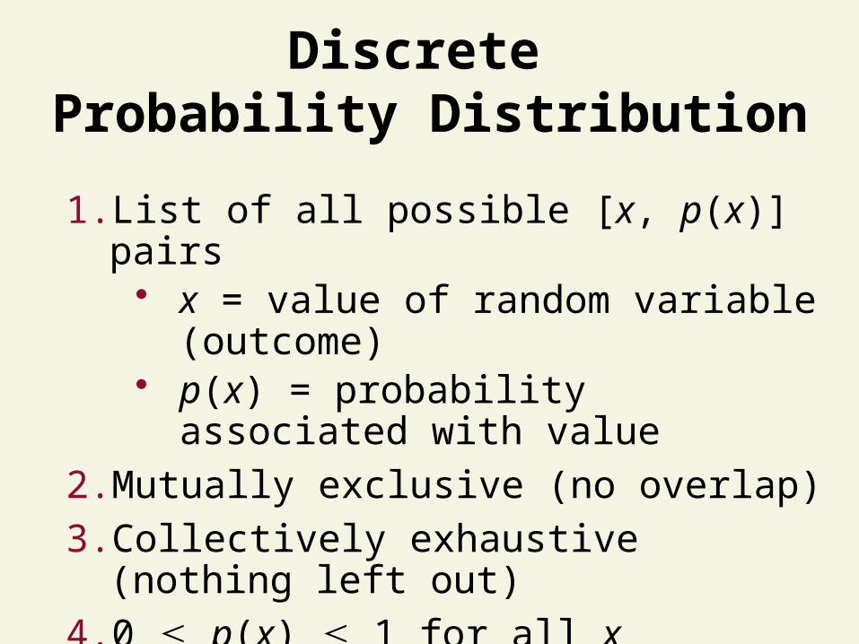
Discrete Probability Distribution
1. List of all possible [x, p(x)] pairs• x = value of random variable (outcome)• p(x) = probability associated with value
2. Mutually exclusive (no overlap)
3. Collectively exhaustive (nothing left out)
4. 0 p(x) 1 for all x
5. p(x) = 1
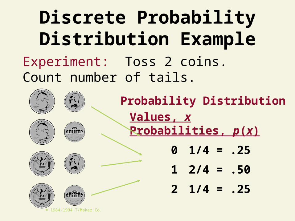
Discrete Probability Distribution Example
Probability Distribution
Values, x Probabilities, p(x)
0 1/4 = .25
1 2/4 = .50
2 1/4 = .25
Experiment: Toss 2 coins. Count number of tails.
© 1984-1994 T/Maker Co.
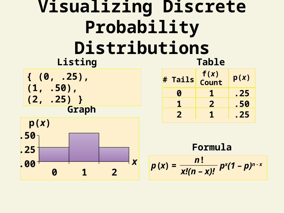
Visualizing Discrete Probability Distributions
Listing Table
Formula
# Tailsf(x)
Countp(x)
0 1 .251 2 .502 1 .25
p xn
x!(n – x)!( )
!= px(1 – p)n - x
Graph
.00
.25
.50
0 1 2x
p(x)
{ (0, .25), (1, .50), (2, .25) }
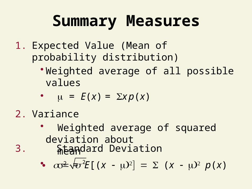
Summary Measures
1. Expected Value (Mean of probability distribution)•Weighted average of all possible values• = E(x) = x p(x)
2. Variance• Weighted average of squared deviation about
mean • 2 = E[(x (x p(x)
3. Standard Deviation2 ●
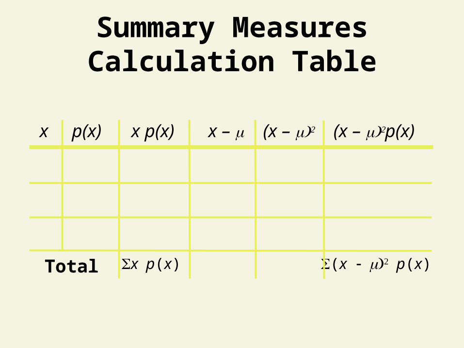
Summary Measures Calculation Table
x p(x) x p(x) x –
Total (x p(x)
(x – )2 (x – )2p(x)
xp(x)
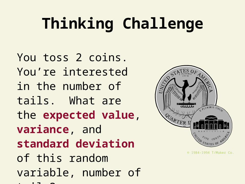
Thinking Challenge
You toss 2 coins. You’re interested in the number of tails. What are the expected value, variance, and standard deviation of this random variable, number of tails?
© 1984-1994 T/Maker Co.
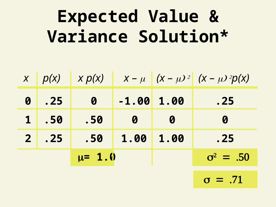
Expected Value & Variance Solution*
0 .25 -1.00 1.00
1 .50 0 0
2 .25 1.00 1.00
0
.50
.50
= 1.0
x p(x) x p(x) x – (x – ) 2 (x – ) 2p(x)
.25
0
.25
2 = .50
= .71
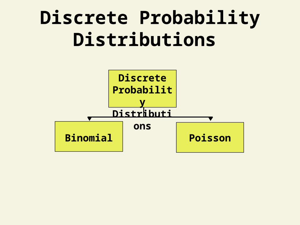
Discrete Probability Distributions
Discrete Probability
Distributions
Binomial Poisson
Binomial Distribution
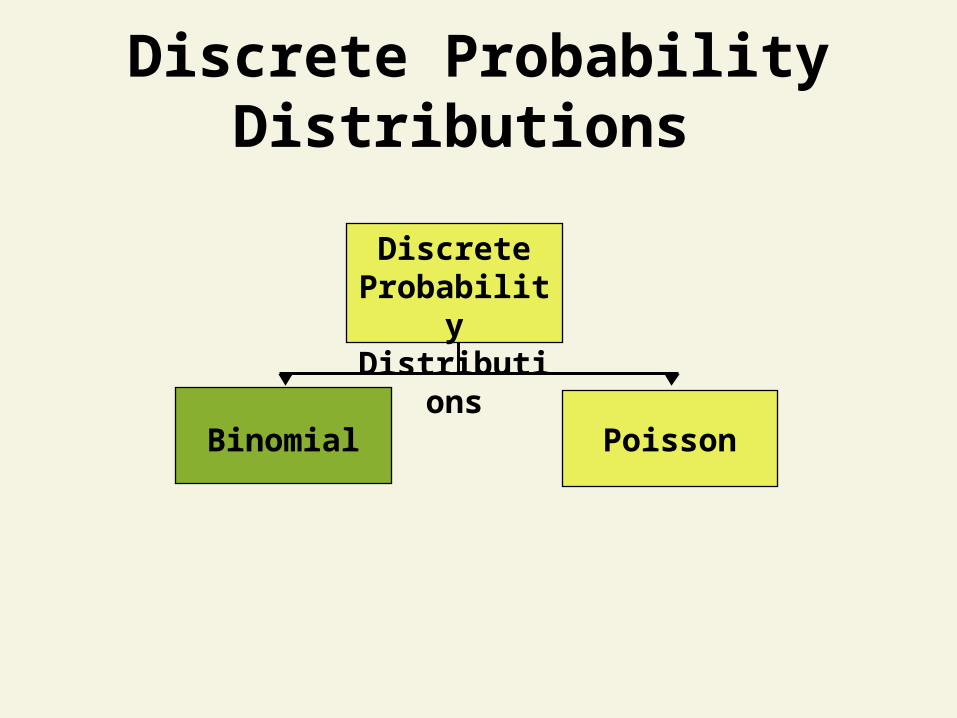
Discrete Probability Distributions
Discrete Probability
Distributions
Binomial Poisson
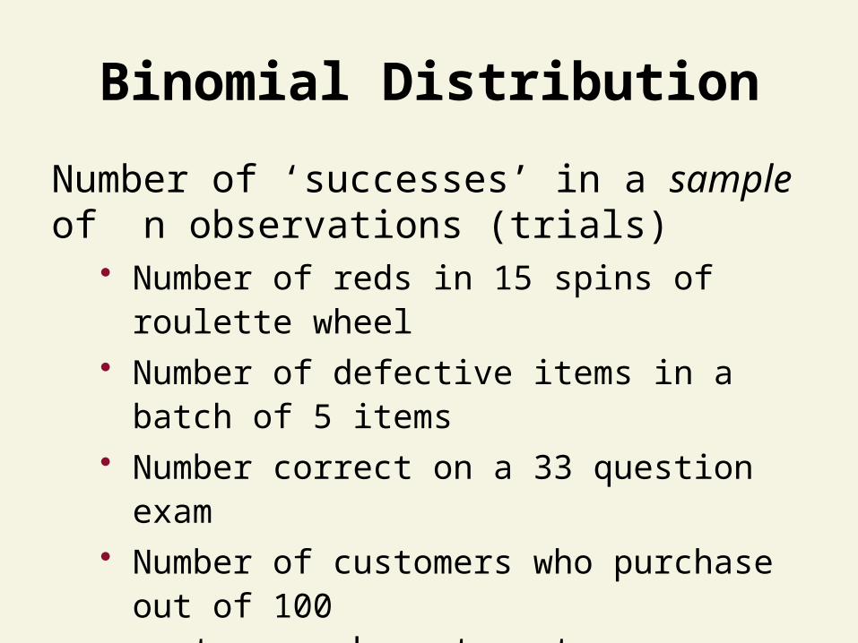
Binomial Distribution
Number of ‘successes’ in a sample of n observations (trials)
• Number of reds in 15 spins of roulette wheel• Number of defective items in a batch of 5 items• Number correct on a 33 question exam• Number of customers who purchase out of 100
customers who enter store
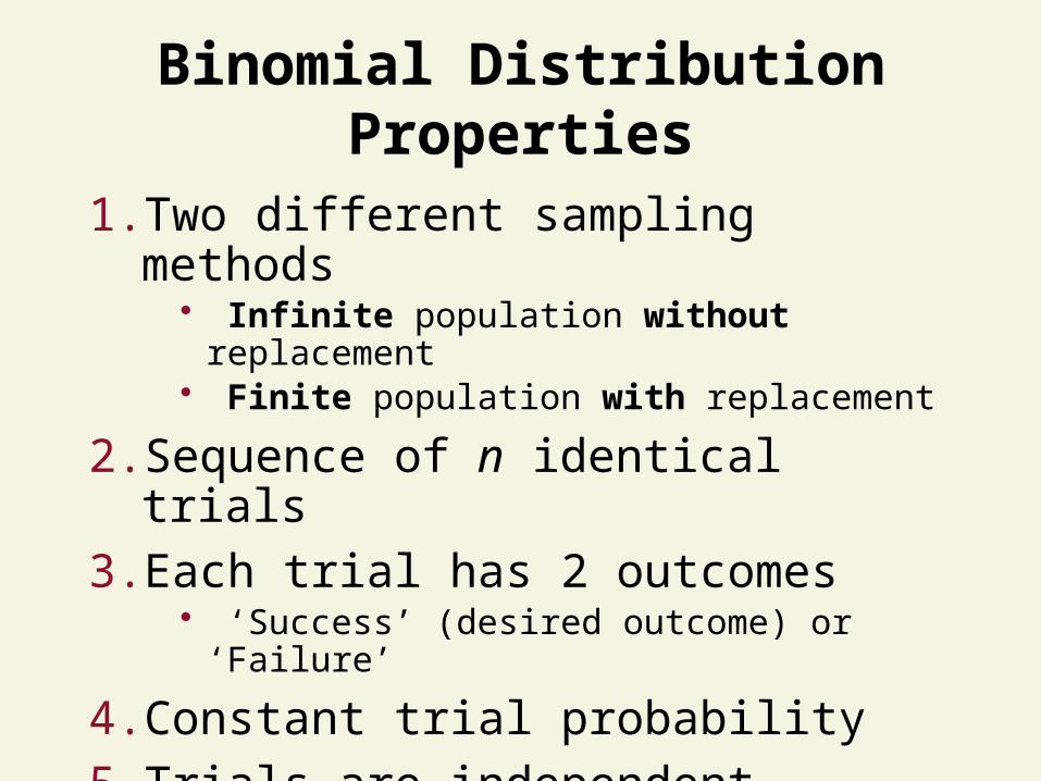
Binomial Distribution Properties
1. Two different sampling methods• Infinite population without replacement• Finite population with replacement
2. Sequence of n identical trials
3. Each trial has 2 outcomes• ‘Success’ (desired outcome) or ‘Failure’
4. Constant trial probability
5. Trials are independent
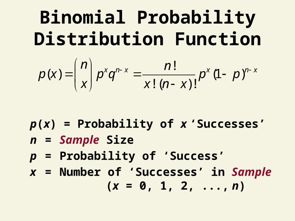
Binomial Probability Distribution Function
!( ) (1 )
! ( )!x n x x n xn n
p x p q p px x n x
p(x) = Probability of x ‘Successes’
n = Sample Size
p = Probability of ‘Success’
x = Number of ‘Successes’ in Sample (x = 0, 1, 2, ..., n)
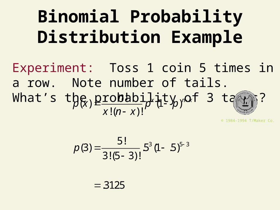
Binomial Probability Distribution Example
3 5 3
!( ) (1 )
!( )!
5!(3) .5 (1 .5)
3!(5 3)!
.3125
x n xnp x p p
x n x
p
Experiment: Toss 1 coin 5 times in a row. Note number of tails. What’s the probability of 3 tails?
© 1984-1994 T/Maker Co.
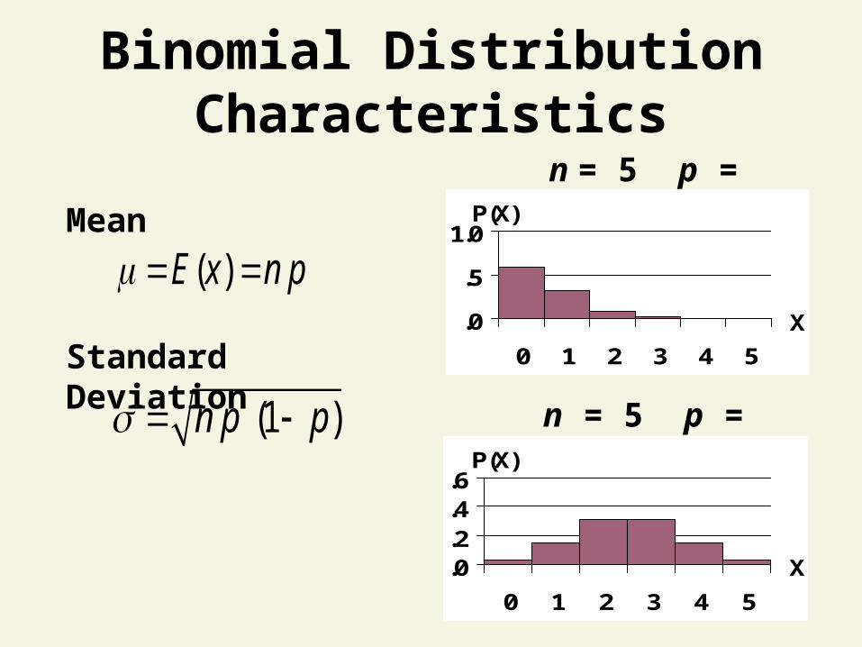
Binomial Distribution Characteristics
.0
.5
1.0
0 1 2 3 4 5
X
P(X)
.0
.2
.4
.6
0 1 2 3 4 5
X
P(X)
n = 5 p = 0.1
n = 5 p = 0.5
( )E x n p Mean
Standard Deviation
(1 )n p p
Binomial Distribution Thinking Challenge
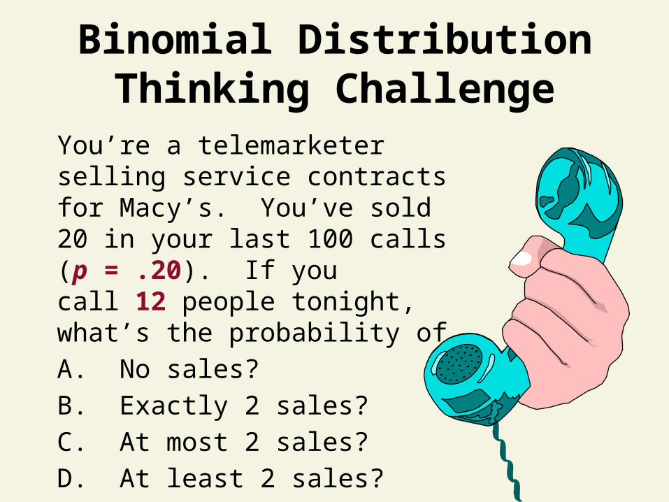
You’re a telemarketer selling service contracts for Macy’s. You’ve sold 20 in your last 100 calls (p = .20). If you call 12 people tonight, what’s the probability of
A. No sales?
B. Exactly 2 sales?
C. At most 2 sales?
D. At least 2 sales?
Binomial Distribution Solution*
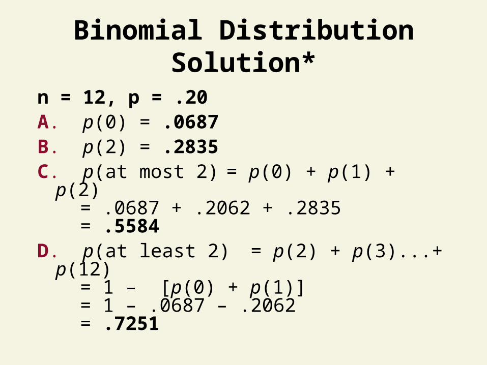
n = 12, p = .20A. p(0) = .0687 B. p(2) = .2835C. p(at most 2) = p(0) + p(1) + p(2)
= .0687 + .2062 + .2835= .5584
D. p(at least 2) = p(2) + p(3)...+ p(12)= 1 – [p(0) + p(1)] = 1 – .0687 – .2062= .7251
Poisson Distribution
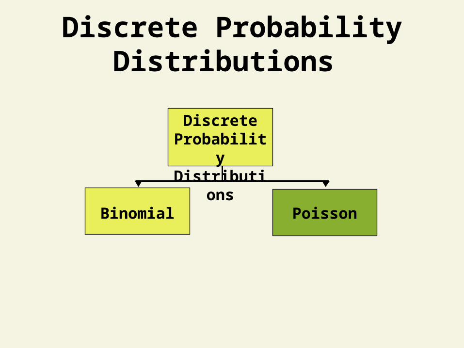
Discrete Probability Distributions
Discrete Probability
Distributions
Binomial Poisson
Poisson Distribution
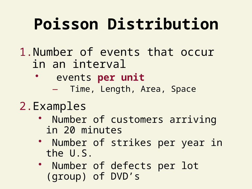
1. Number of events that occur in an interval • events per unit
— Time, Length, Area, Space
2. Examples• Number of customers arriving in 20 minutes• Number of strikes per year in the U.S.• Number of defects per lot (group) of DVD’s
Poisson Process
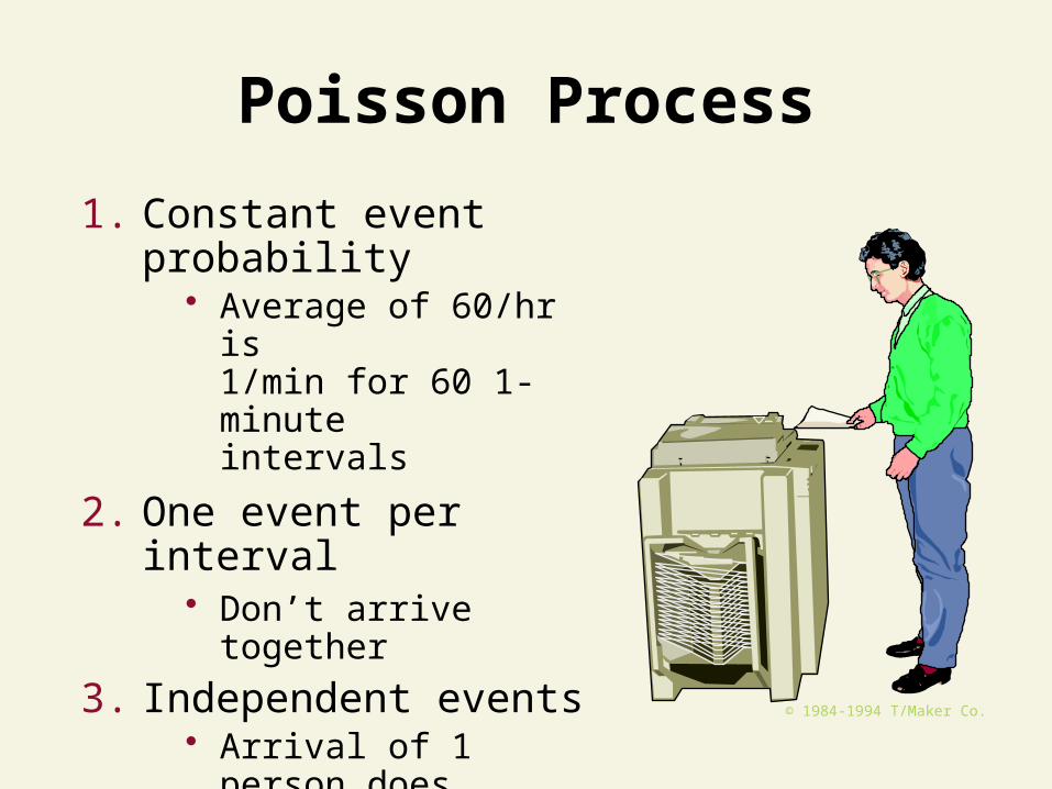
1. Constant event probability
• Average of 60/hr is1/min for 60 1-minuteintervals
2. One event per interval• Don’t arrive together
3. Independent events• Arrival of 1 person does
not affect another’sarrival
© 1984-1994 T/Maker Co.
Poisson Probability Distribution Function
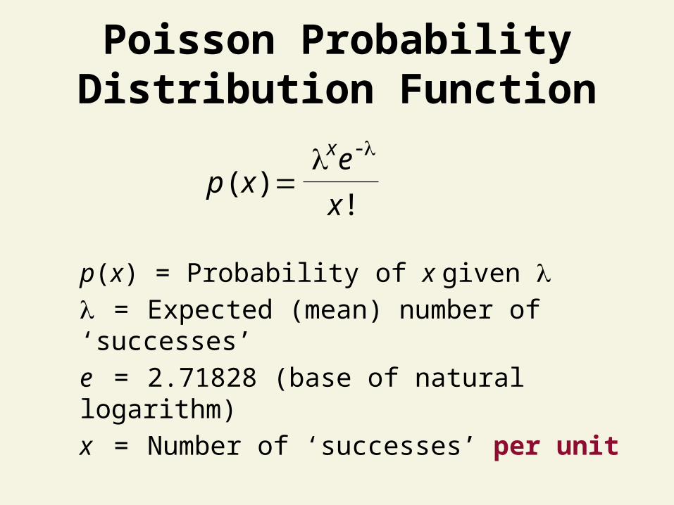
p(x) = Probability of x given = Expected (mean) number of ‘successes’
e = 2.71828 (base of natural logarithm)
x = Number of ‘successes’ per unit
p xx
( )!
x e -
Poisson Distribution Characteristics
.0
.2
.4
.6
.8
0 1 2 3 4 5
X
P(X)
.0
.1
.2
.3
X
P(X)
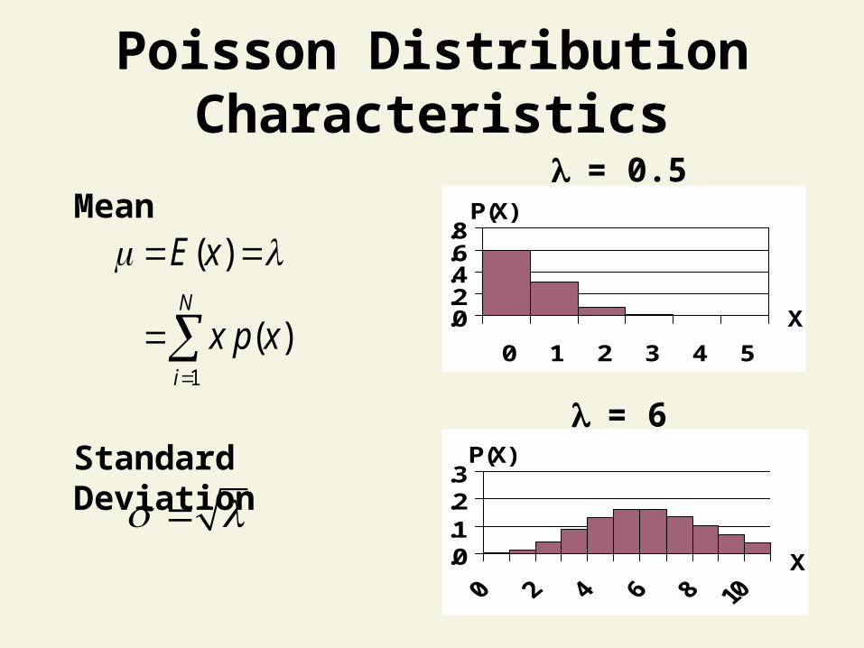
= 0.5
= 6
Mean
Standard Deviation
1
( )
( )N
i
E x
x p x
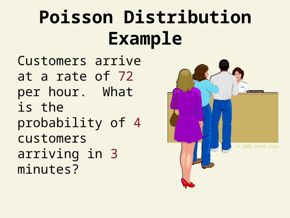
Poisson Distribution Example
Customers arrive at a rate of 72 per hour. What is the probability of 4 customers arriving in 3 minutes?
© 1995 Corel Corp.
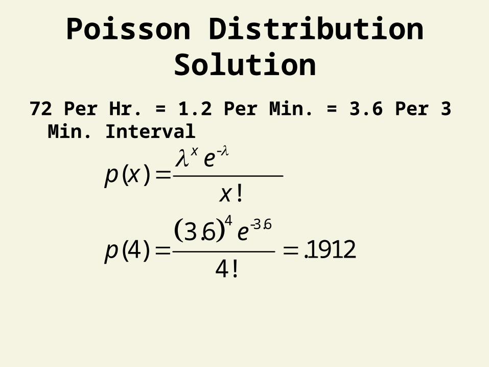
Poisson Distribution Solution
72 Per Hr. = 1.2 Per Min. = 3.6 Per 3 Min. Interval
-
4 -3.6
( )!
3.6(4) .1912
4!
x ep x
x
ep

Thinking Challenge
You work in Quality Assurance for an investment firm. A clerk enters 75 words per minute with 6 errors per hour. What is the probability of 0 errors in a 255-word bond transaction?
© 1984-1994 T/Maker Co.
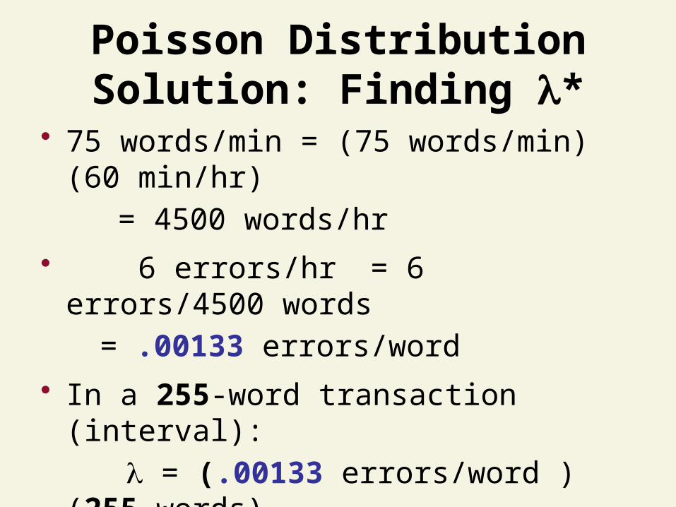
Poisson Distribution Solution: Finding *
• 75 words/min = (75 words/min)(60 min/hr)
= 4500 words/hr
• 6 errors/hr = 6 errors/4500 words
= .00133 errors/word
• In a 255-word transaction (interval):
= (.00133 errors/word )(255 words)
= .34 errors/255-word transaction
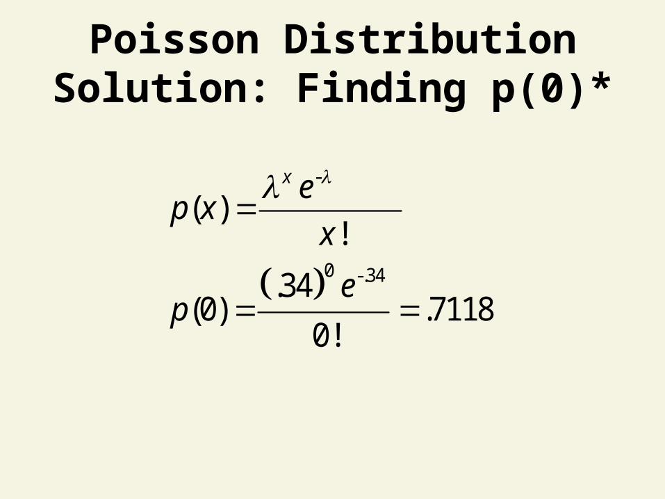
Poisson Distribution Solution: Finding p(0)*
-
0 -.34
( )!
.34(0) .7118
0!
x ep x
x
ep
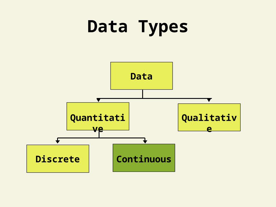
Data Types
Data
Quantitative Qualitative
ContinuousDiscrete
Probability Distributions for Continuous Random
Variables
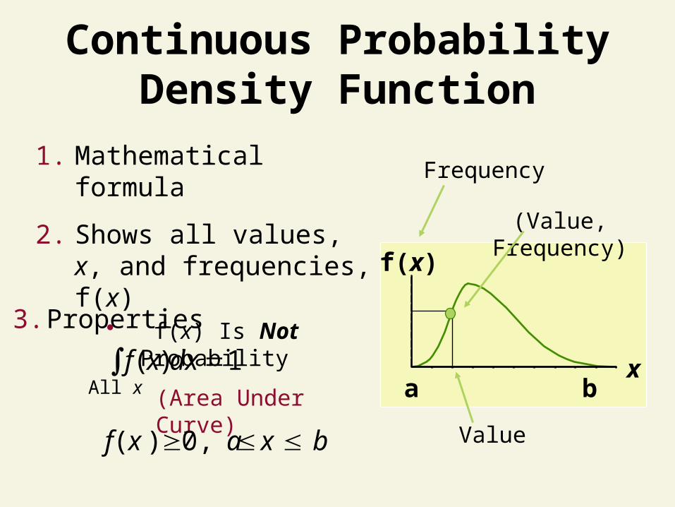
Continuous Probability Density Function
1. Mathematical formula
2. Shows all values, x, and frequencies, f(x)
• f(x) Is Not Probability
Value
(Value, Frequency)
Frequency
f(x)
a bx
(Area Under Curve)
f x dx
f x
( )
( )
All x
a x b
1
0,
3. Properties
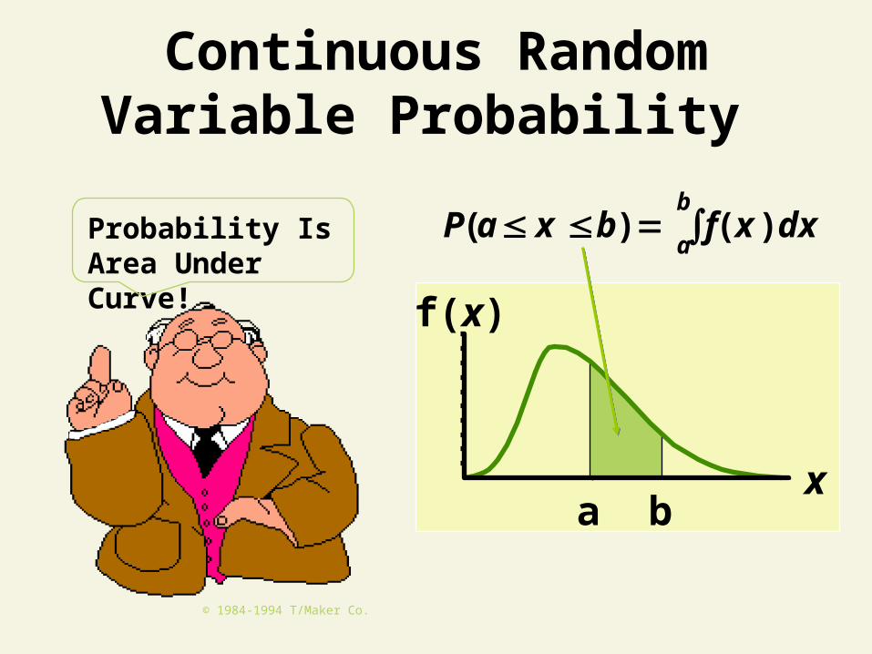
Continuous Random Variable Probability
Probability Is Area Under Curve!
© 1984-1994 T/Maker Co.
P a x b f x dxa
b( ) ( )
f(x)
xa b
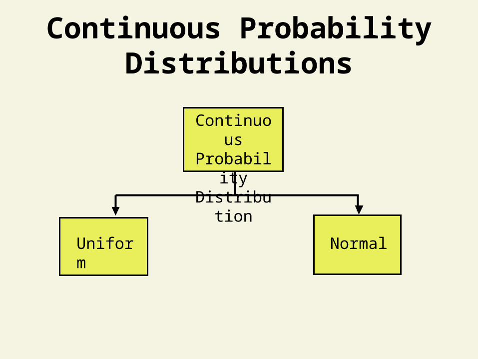
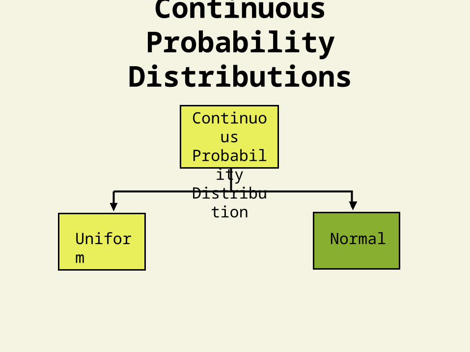
Continuous Probability Distributions
ContinuousProbabilityDistribution
Uniform Normal
Uniform Distribution
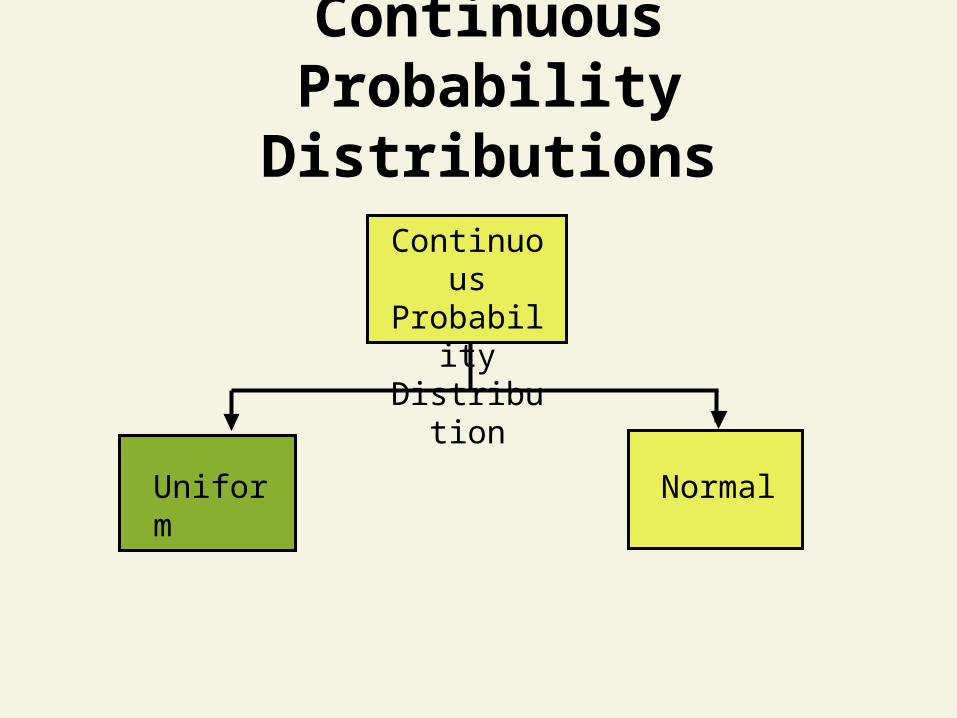
Continuous Probability Distributions
ContinuousProbabilityDistribution
Uniform Normal
1d c
x
f(x)
dc a b
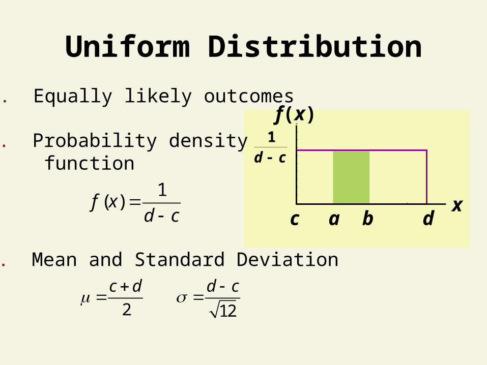
Uniform Distribution
2 12
c d d c
3. Mean and Standard Deviation
1( )f x
d c
2. Probability density function
1. Equally likely outcomes
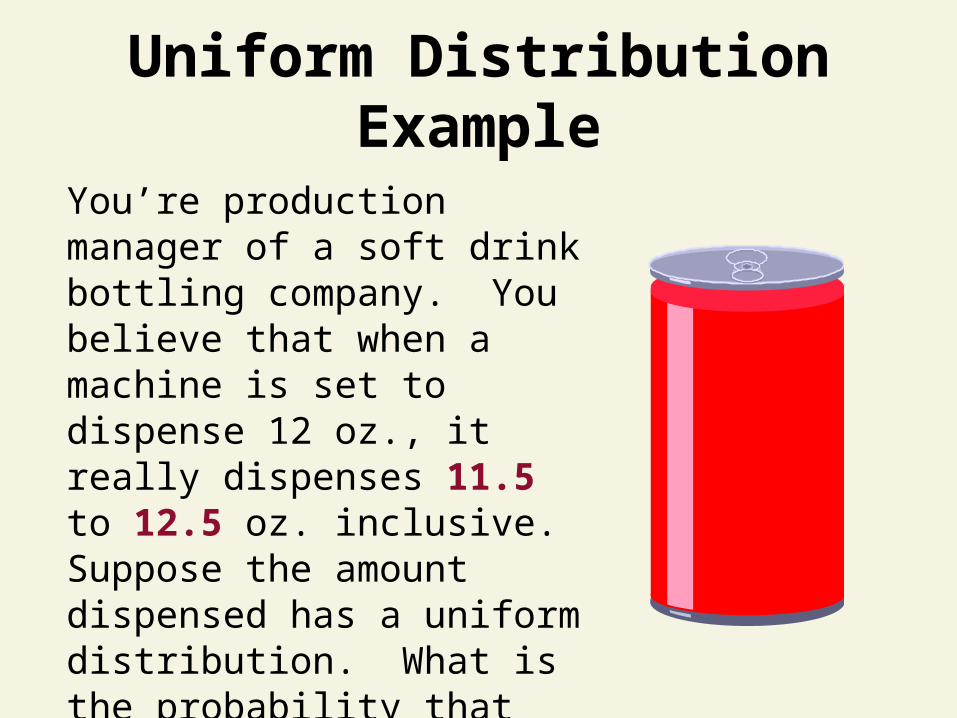
Uniform Distribution Example
You’re production manager of a soft drink bottling company. You believe that when a machine is set to dispense 12 oz., it really dispenses 11.5 to 12.5 oz. inclusive. Suppose the amount dispensed has a uniform distribution. What is the probability that less than 11.8 oz. is dispensed?
SODA
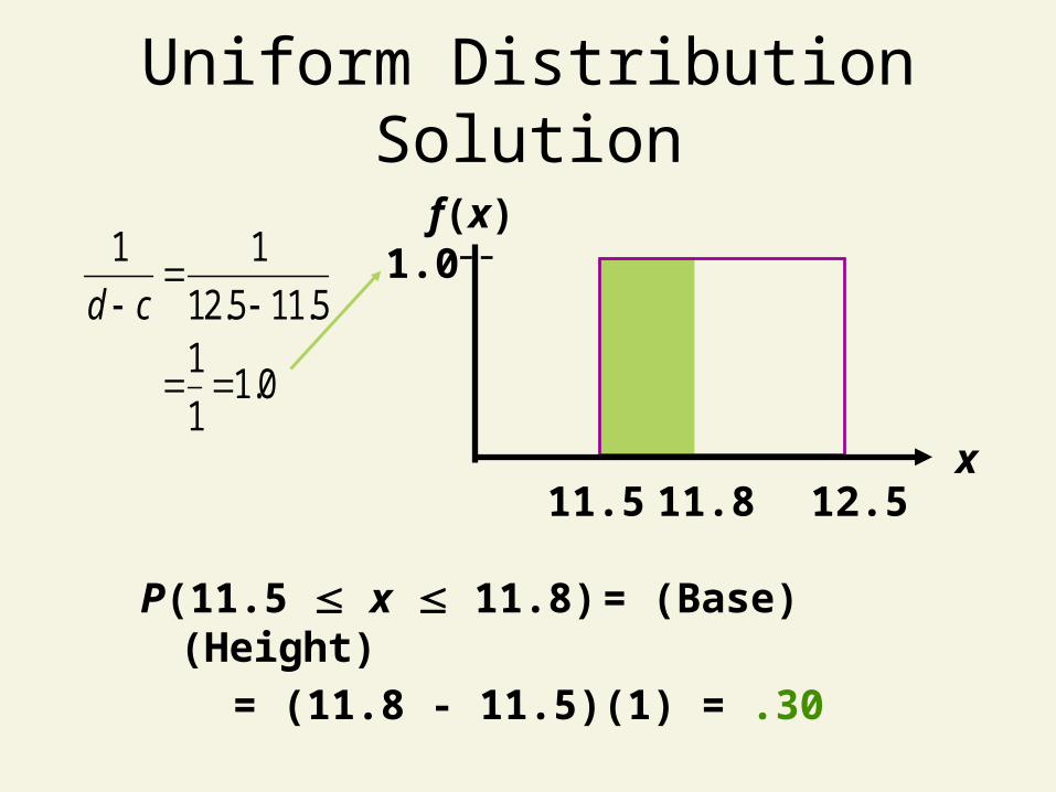
Uniform Distribution Solution
P(11.5 x 11.8) = (Base)(Height)
= (11.8 - 11.5)(1) = .30
11.5 12.5
f(x)
x11.8
1 1
12.5 11.51
1.01
d c
1.0

Normal Distribution
Continuous Probability Distributions
ContinuousProbabilityDistribution
Uniform Normal
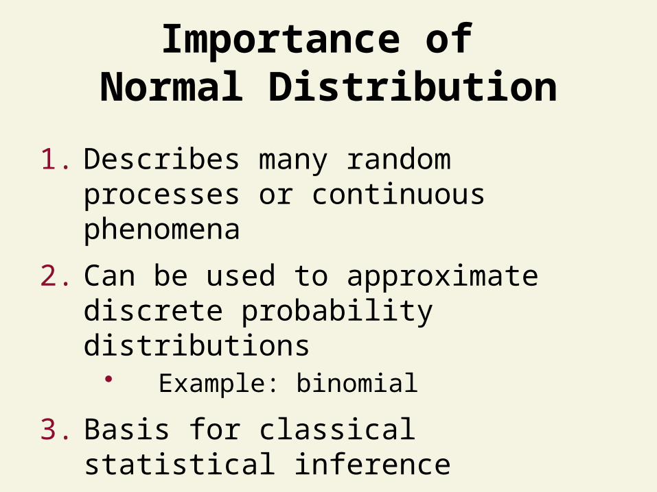
Importance of Normal Distribution
1. Describes many random processes or continuous phenomena
2. Can be used to approximate discrete probability distributions• Example: binomial
3. Basis for classical statistical inference
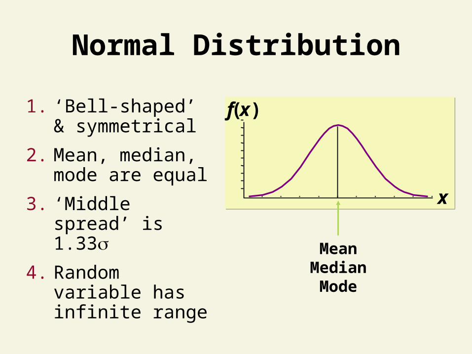
Normal Distribution
1. ‘Bell-shaped’ & symmetrical
2. Mean, median, mode are equal
3. ‘Middle spread’ is 1.33
4. Random variable has infinite range
x
f(x )
Mean Median Mode
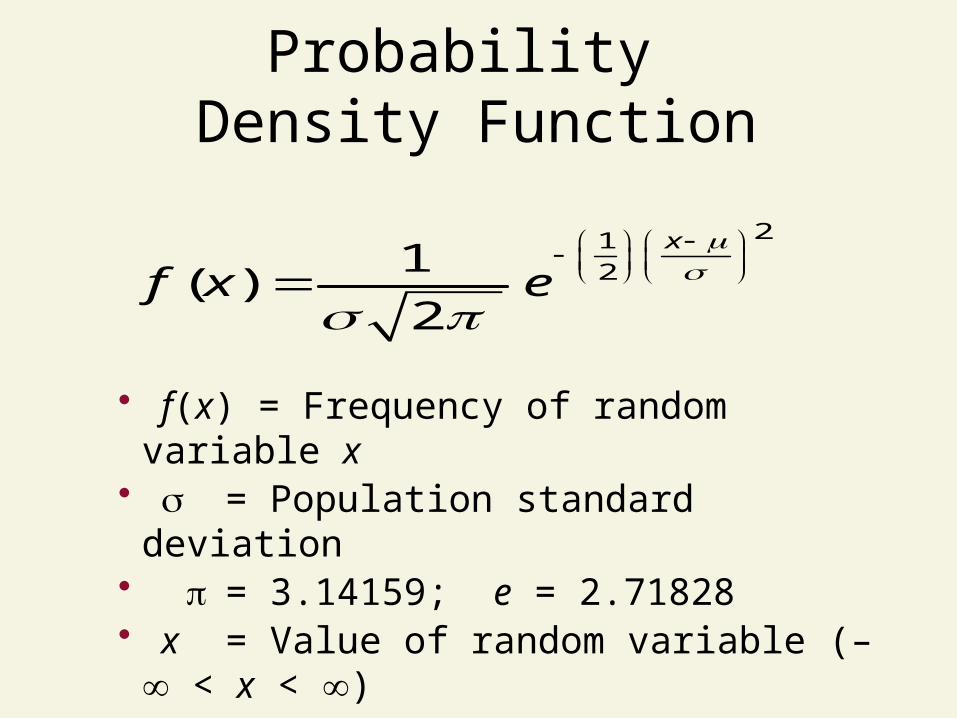
Probability Density Function
21
21( )
2
x
f x e
• f(x) = Frequency of random variable x• = Population standard deviation • = 3.14159; e = 2.71828• x = Value of random variable (– < x < )• = Population mean
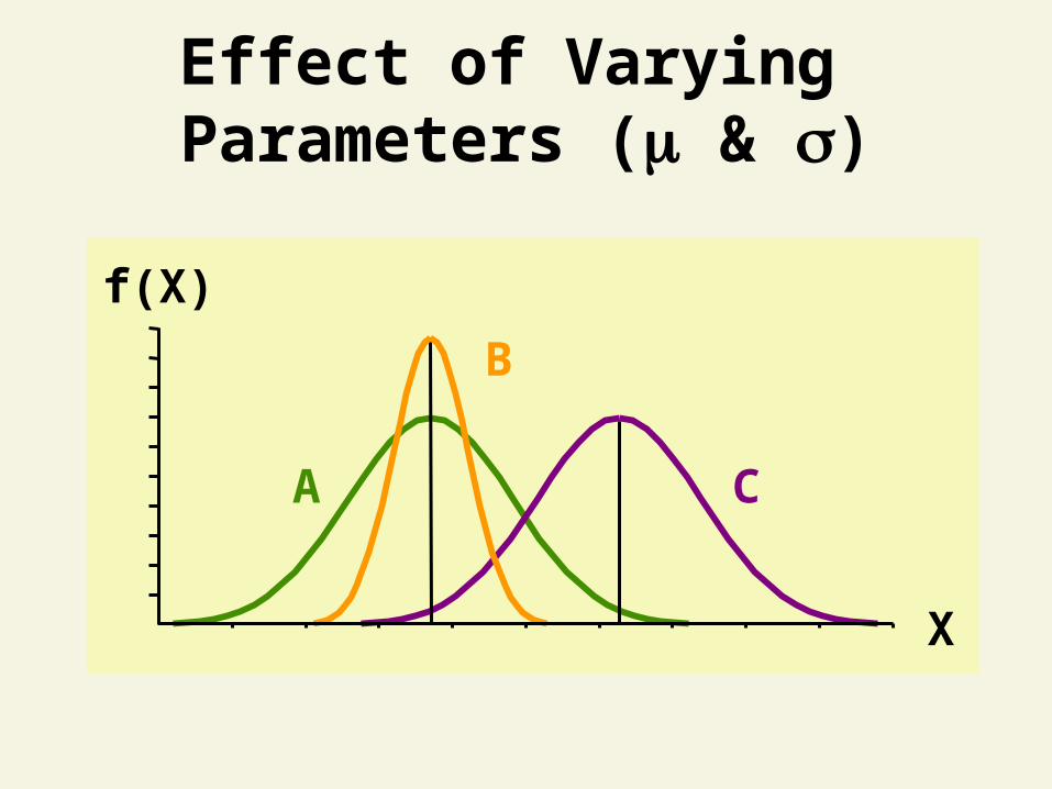
Effect of Varying Parameters ( & )
X
f(X)
CA
B
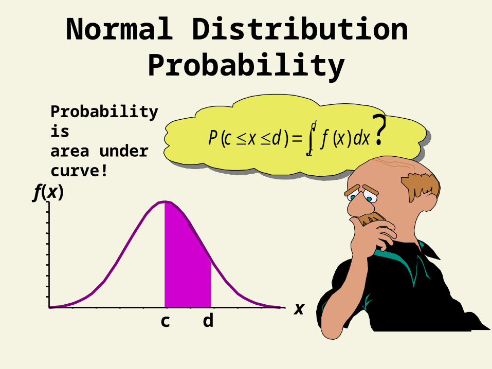
Normal Distribution Probability
?)()( dxxfdxcPd
c
c dx
f(x)
Probability is area under curve!
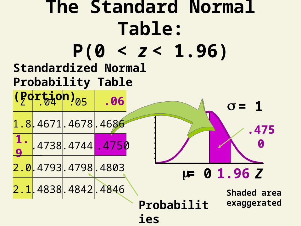
Zm= 0
s = 1
1.96
Z .04 .05
1.8 .4671 .4678 .4686
.4738 .4744
2.0 .4793 .4798 .4803
2.1 .4838 .4842 .4846
The Standard Normal Table:P(0 < z < 1.96)
.06
1.9 .4750
Standardized Normal Probability Table (Portion)
Probabilities
.4750
Shaded area exaggerated
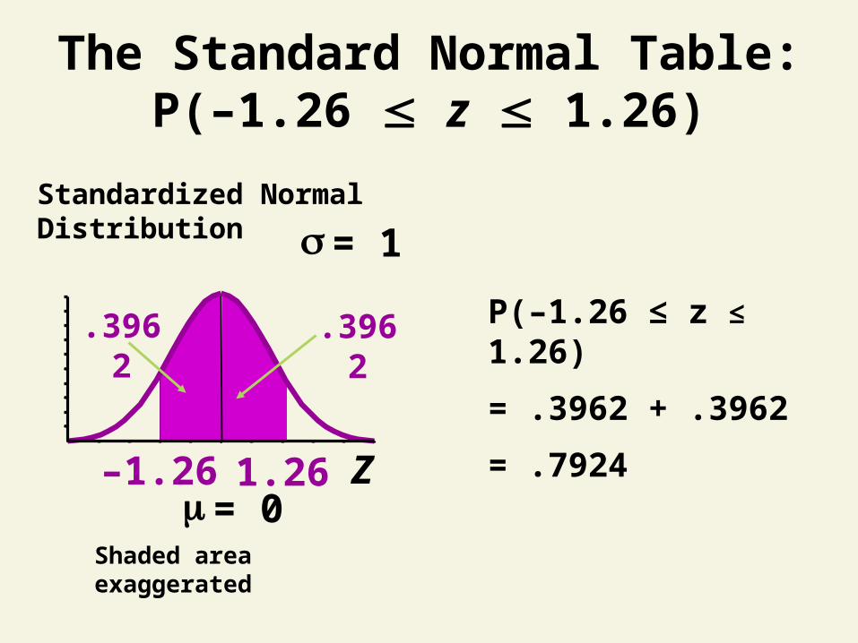
The Standard Normal Table:P(–1.26 z 1.26)
Zm = 0
s = 1
–1.26
Standardized Normal Distribution
Shaded area exaggerated
.3962
1.26
.3962 P(–1.26 ≤ z ≤ 1.26)
= .3962 + .3962
= .7924
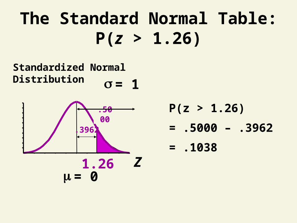
The Standard Normal Table:P(z > 1.26)
Zm = 0
s = 1Standardized Normal Distribution
1.26
P(z > 1.26)
= .5000 – .3962
= .1038
.3962
.5000
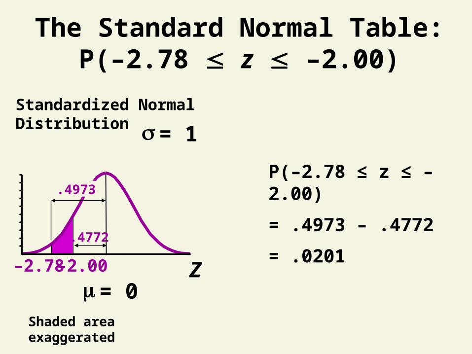
The Standard Normal Table:P(–2.78 z –2.00)
s = 1
m = 0–2.78 Z–2.00
.4973
.4772
Standardized Normal Distribution
Shaded area exaggerated
P(–2.78 ≤ z ≤ –2.00)
= .4973 – .4772
= .0201
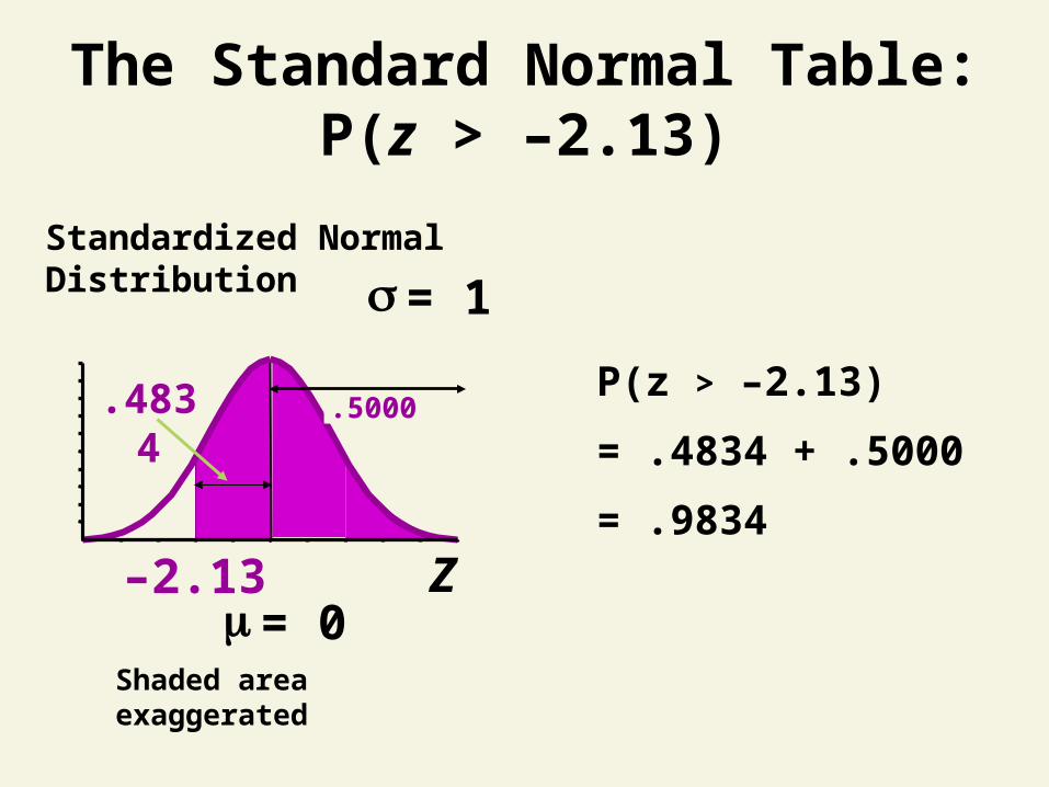
The Standard Normal Table:P(z > –2.13)
Zm = 0
s = 1
–2.13
Standardized Normal Distribution
Shaded area exaggerated
P(z > –2.13)
= .4834 + .5000
= .9834
.5000.4834
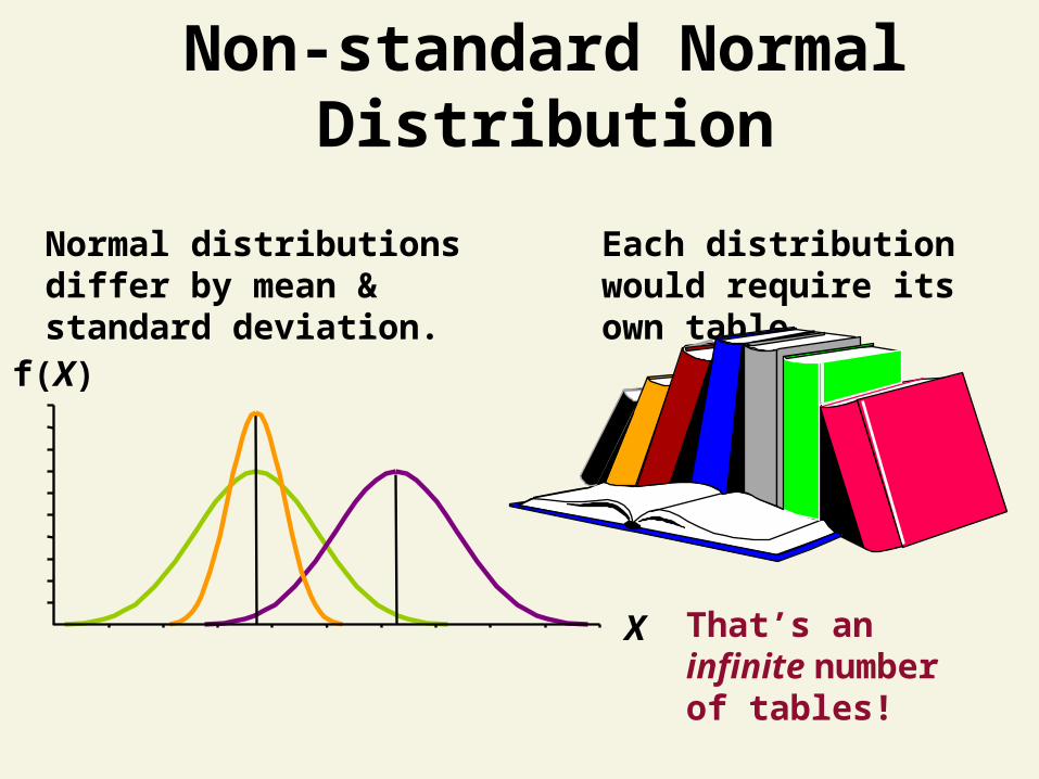
X
f(X)
Non-standard Normal Distribution
Normal distributions differ by mean & standard deviation.
Each distribution would require its own table.
That’s an infinite number of tables!
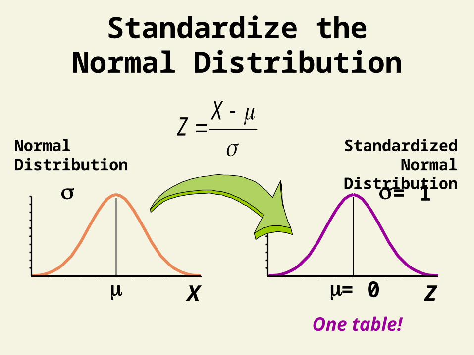
Standardize theNormal Distribution
Normal Distribution
Xm
s
One table!
m = 0
s = 1
Z
Standardized Normal Distribution
XZ
Zm= 0
s = 1
.12
Standardized Normal Distribution
Shaded area exaggerated
.0478
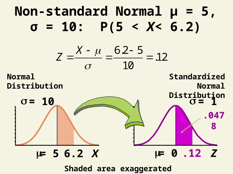
Non-standard Normal μ = 5, σ = 10: P(5 < X< 6.2)
Normal Distribution
Xm= 5
s = 10
6.2
6.2 5.12
10
XZ
Zm = 0
s = 1
-.12
Standardized Normal Distribution
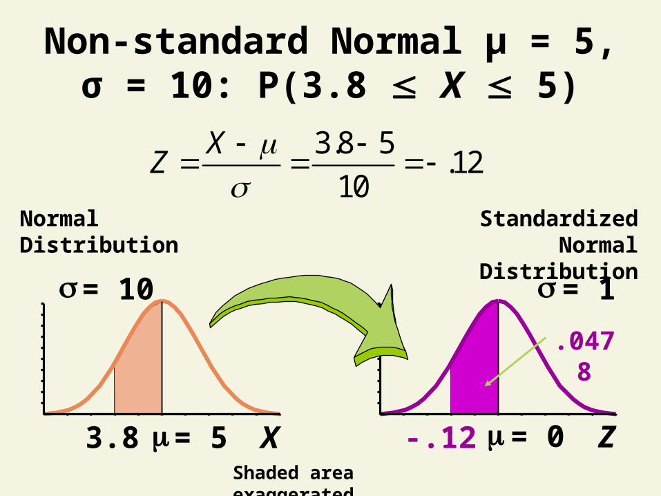
Non-standard Normal μ = 5, σ = 10: P(3.8 X 5)
Normal Distribution
X m = 5
s = 10
3.8
.0478
Shaded area exaggerated
3.8 5.12
10
XZ
0
s = 1
-.21 Z.21
Standardized Normal Distribution
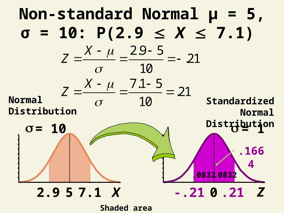
Non-standard Normal μ = 5, σ = 10: P(2.9 X 7.1)
5
s = 10
2.9 7.1 X
Normal Distribution
.1664
.0832.0832
Shaded area exaggerated
2.9 5.21
10
XZ
7.1 5.21
10
XZ
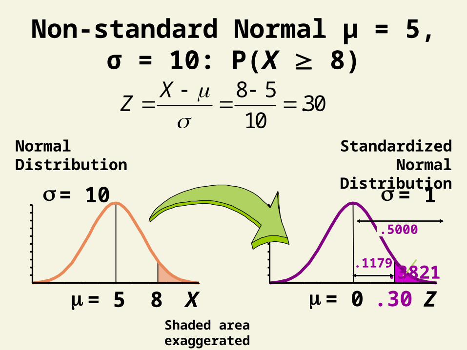
Non-standard Normal μ = 5, σ = 10: P(X 8)
Xm = 5
s = 10
8
Normal Distribution
Z = 0 .30
Standardized Normal Distribution
m
s = 1
.3821.5000
.1179
Shaded area exaggerated
8 5.30
10
XZ
m = 0
s = 1
.30 Z.21
Standardized Normal Distribution
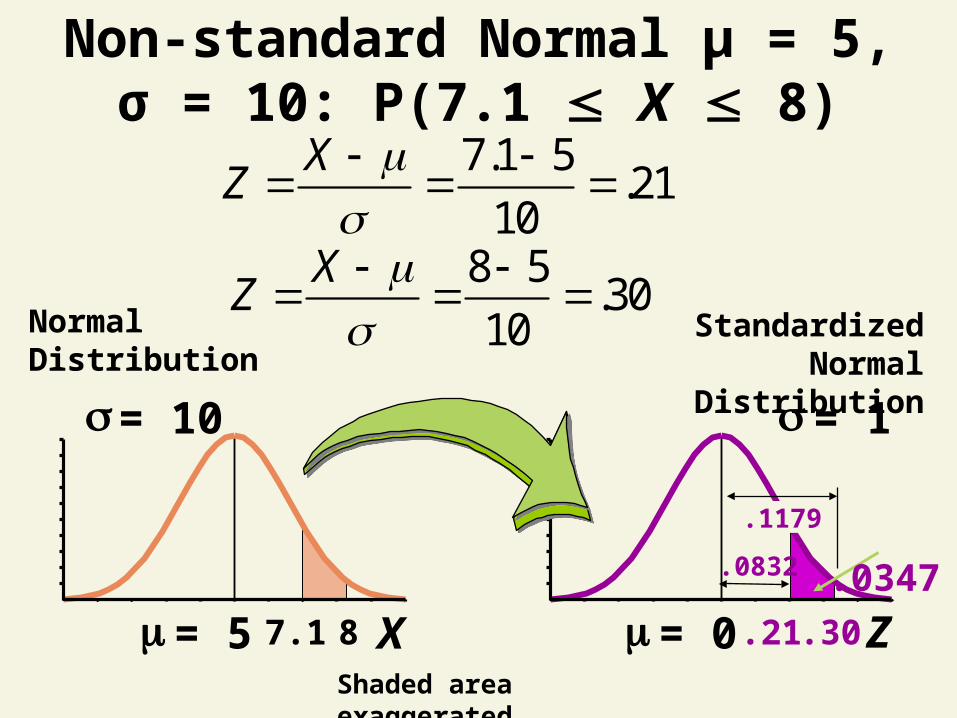
Non-standard Normal μ = 5, σ = 10: P(7.1 X 8)
m = 5
s = 10
87.1 X
Normal Distribution
.1179 .0347.0832
Shaded area exaggerated
7.1 5.21
10
XZ
8 5.30
10
XZ
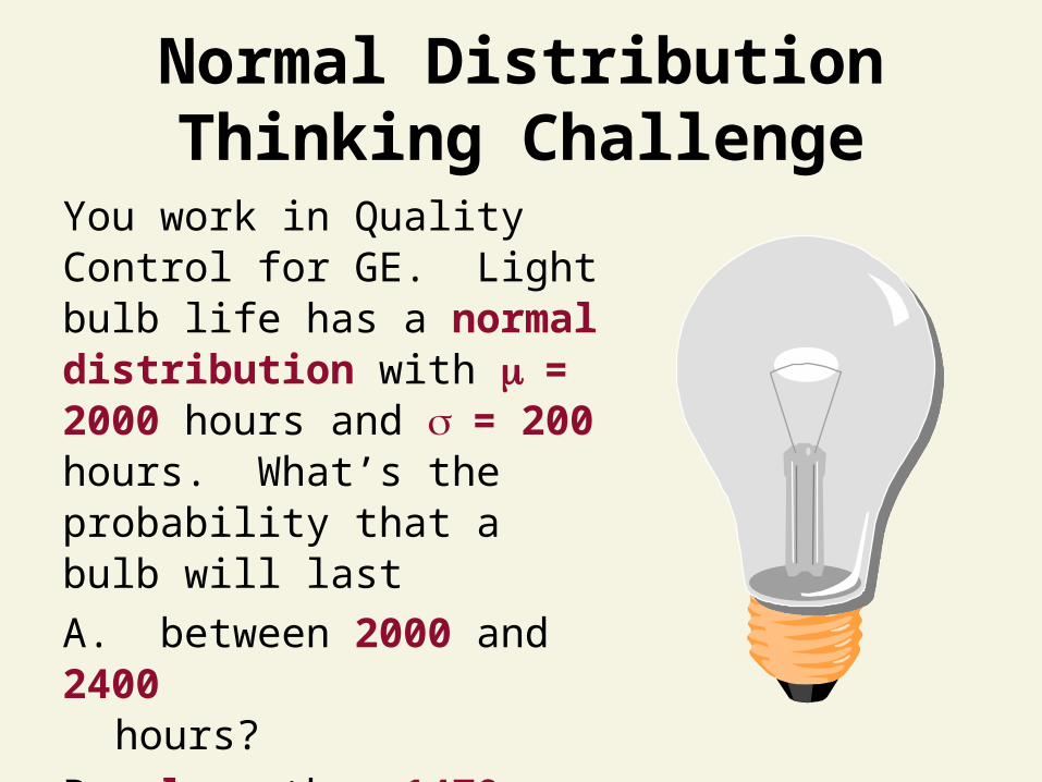
Normal Distribution Thinking Challenge
You work in Quality Control for GE. Light bulb life has a normal distribution with = 2000 hours and = 200 hours. What’s the probability that a bulb will last
A. between 2000 and 2400 hours?
B. less than 1470 hours?
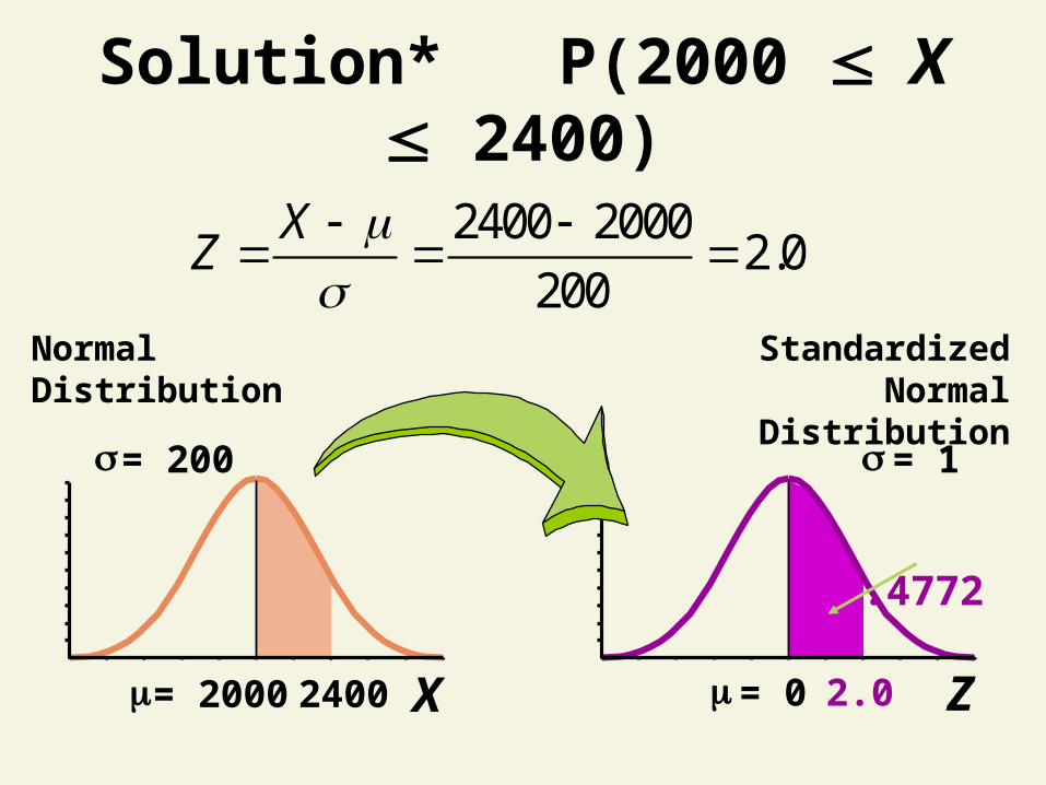
Standardized Normal Distribution
Zm = 0
s = 1
2.0
Solution* P(2000 X 2400)
Normal Distribution
Xm = 2000
s = 200
2400
.4772
2400 20002.0
200
XZ
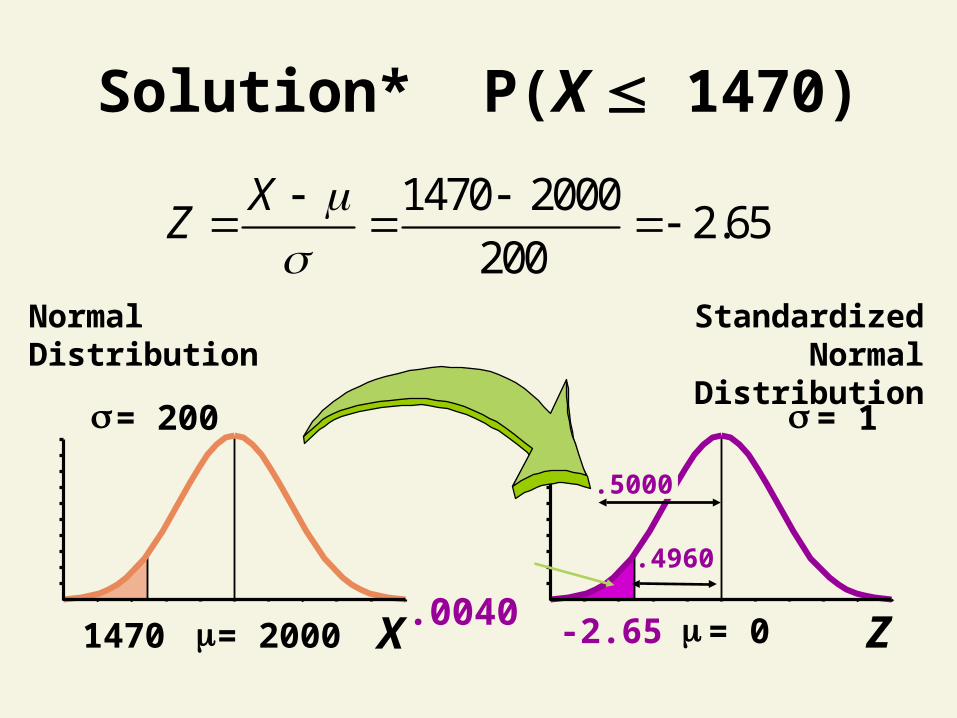
Zm = 0
s = 1
-2.65
Standardized Normal Distribution
Solution* P(X 1470)
Xm = 2000
s = 200
1470
Normal Distribution
.0040 .4960
.5000
1470 20002.65
200
XZ
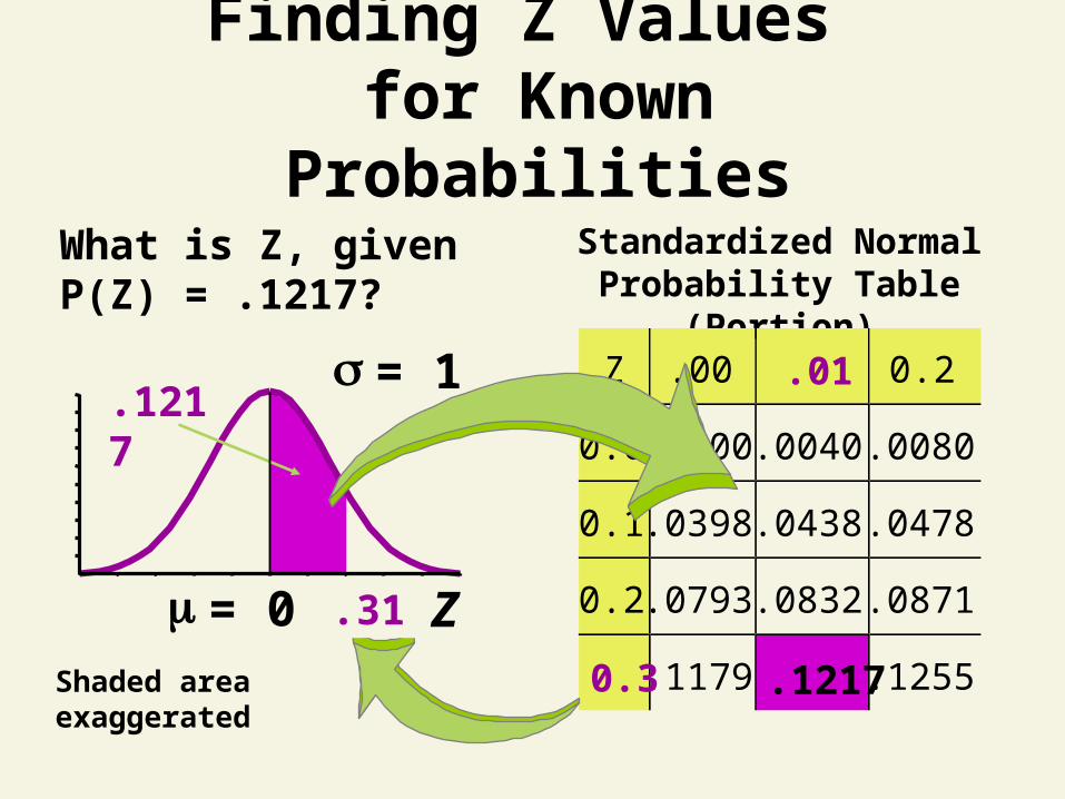
Finding Z Values for Known Probabilities
What is Z, given P(Z) = .1217?
Shaded area exaggerated
Zm = 0
s = 1
?
.1217
Standardized Normal Probability Table (Portion)
Z .00 0.2
0.0 .0000 .0040 .0080
0.1 .0398 .0438 .0478
0.2 .0793 .0832 .0871
.1179 .1255
.01
0.3 .1217
.31
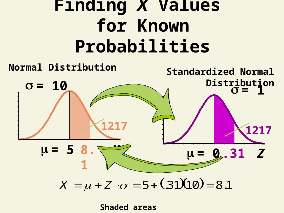
Finding X Values for Known Probabilities
Normal Distribution
X m = 5
s = 10
?
.1217
Standardized Normal Distribution
Shaded areas exaggerated
Zm = 0
s = 1
.31
.1217
1.81031.5 ZX
8.1
Assessing Normality
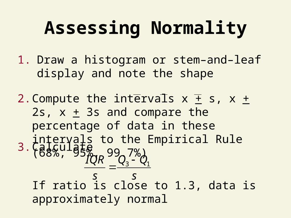
Assessing Normality
1. Draw a histogram or stem–and–leaf display and note the shape
3. Calculate
If ratio is close to 1.3, data is approximately normal
3 1Q QIQR
s s
2. Compute the intervals x + s, x + 2s, x + 3s and compare the percentage of data in these intervals to the Empirical Rule (68%, 95%, 99.7%)
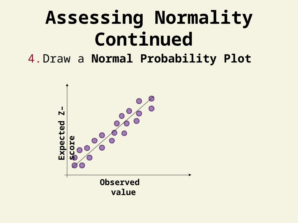
Assessing Normality Continued
Observed value
Exp
ecte
d Z
–sco
re4. Draw a Normal Probability Plot
Normal Approximation of Binomial Distribution
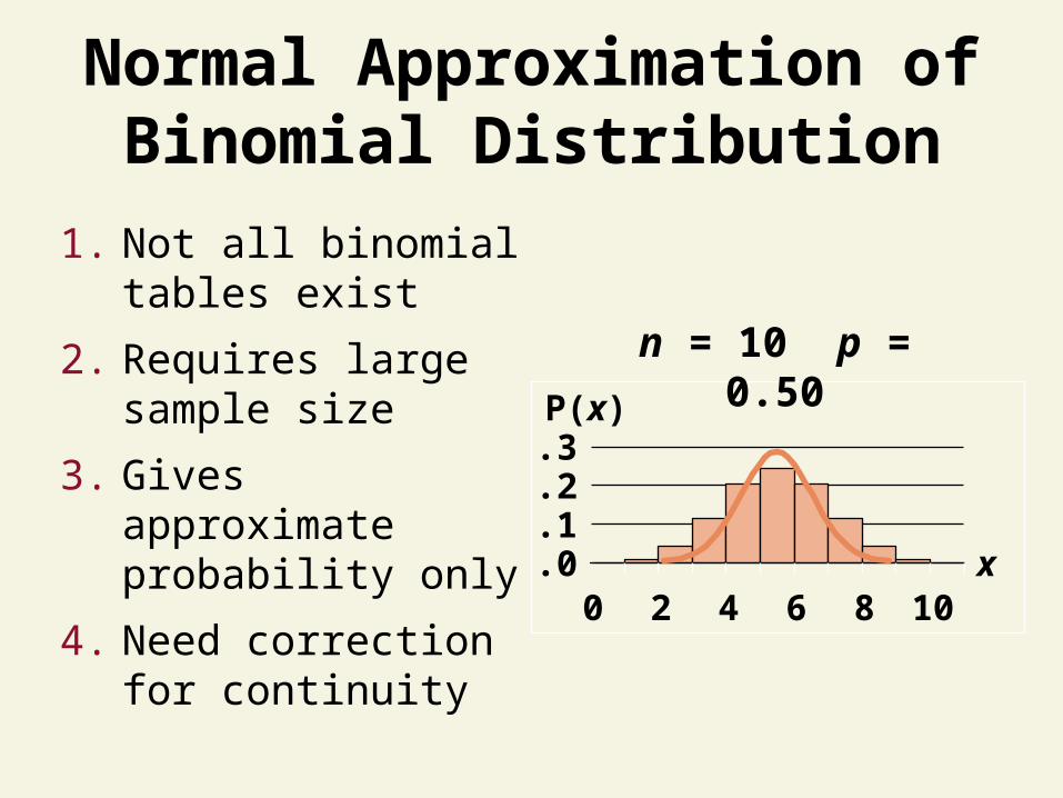
Normal Approximation of Binomial Distribution
1. Not all binomial tables exist
2. Requires large sample size
3. Gives approximate probability only
4. Need correction for continuity
n = 10 p = 0.50
.0
.1
.2
.3
0 2 4 6 8 10x
P(x)
.0
.1
.2
.3
0 2 4 6 8 10
x
P(x)
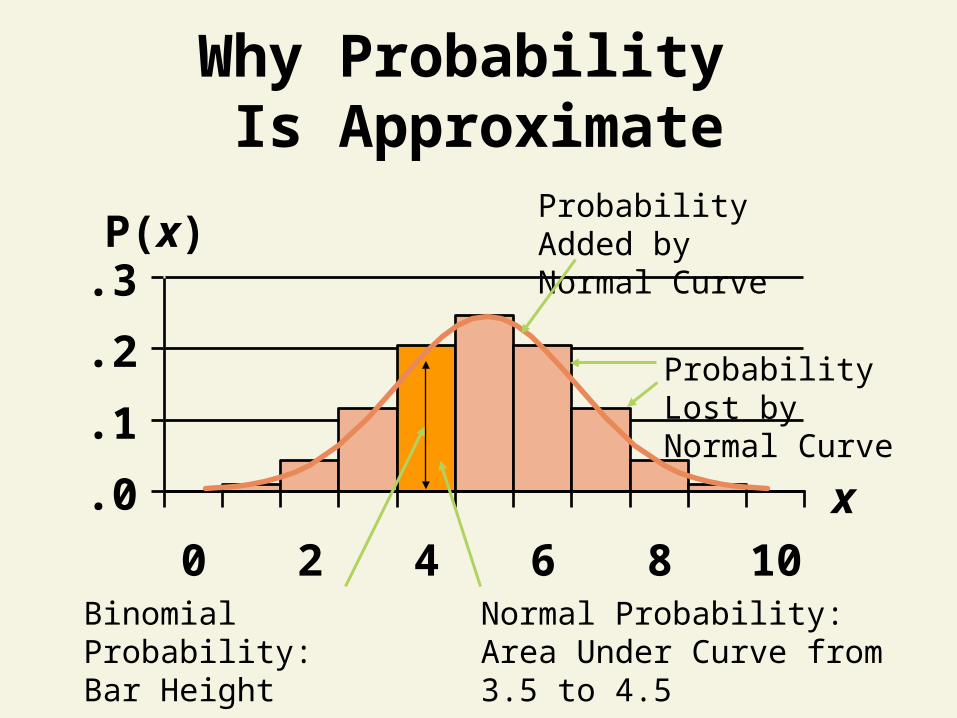
Why Probability Is Approximate
Binomial Probability: Bar Height
Normal Probability: Area Under Curve from 3.5 to 4.5
Probability Added by Normal Curve
Probability Lost by Normal Curve
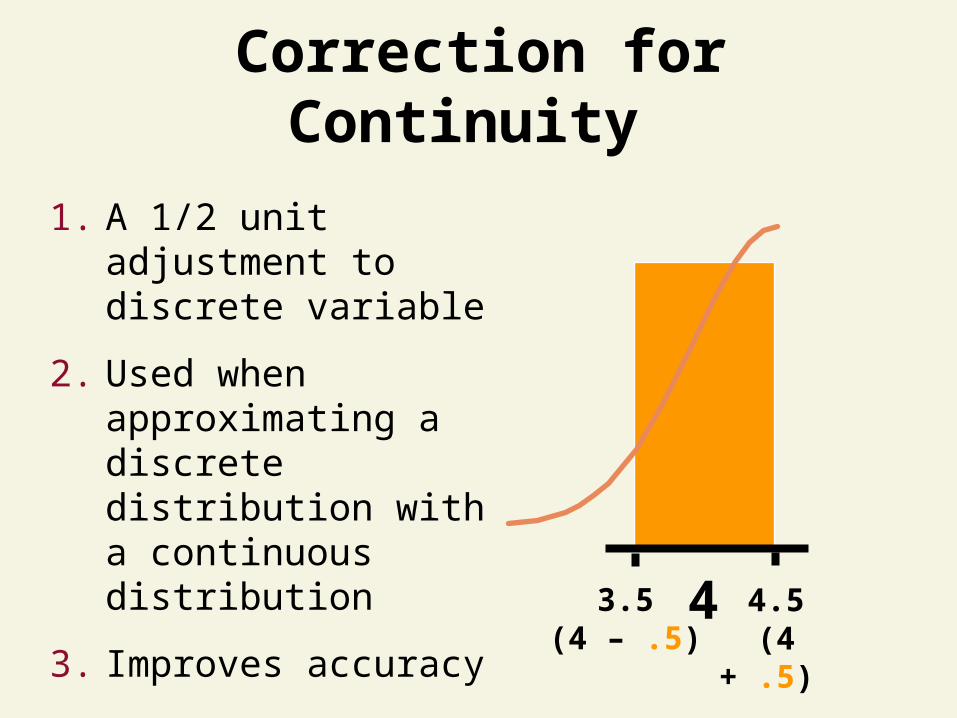
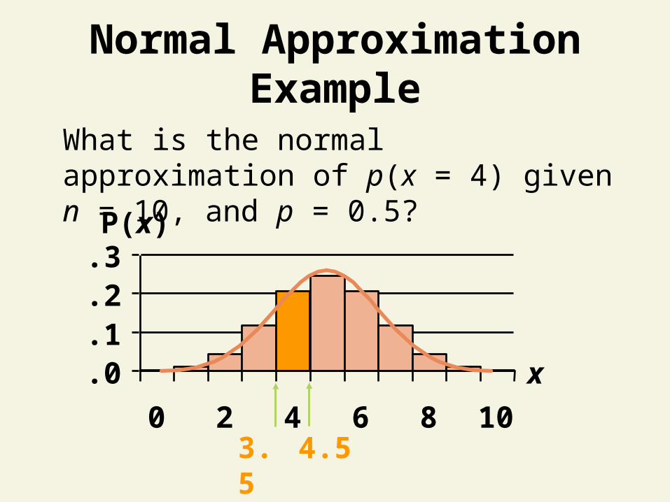
Correction for Continuity
1. A 1/2 unit adjustment to discrete variable
2. Used when approximating a discrete distribution with a continuous distribution
3. Improves accuracy
4.5(4 + .5)
3.5 (4 – .5)
4
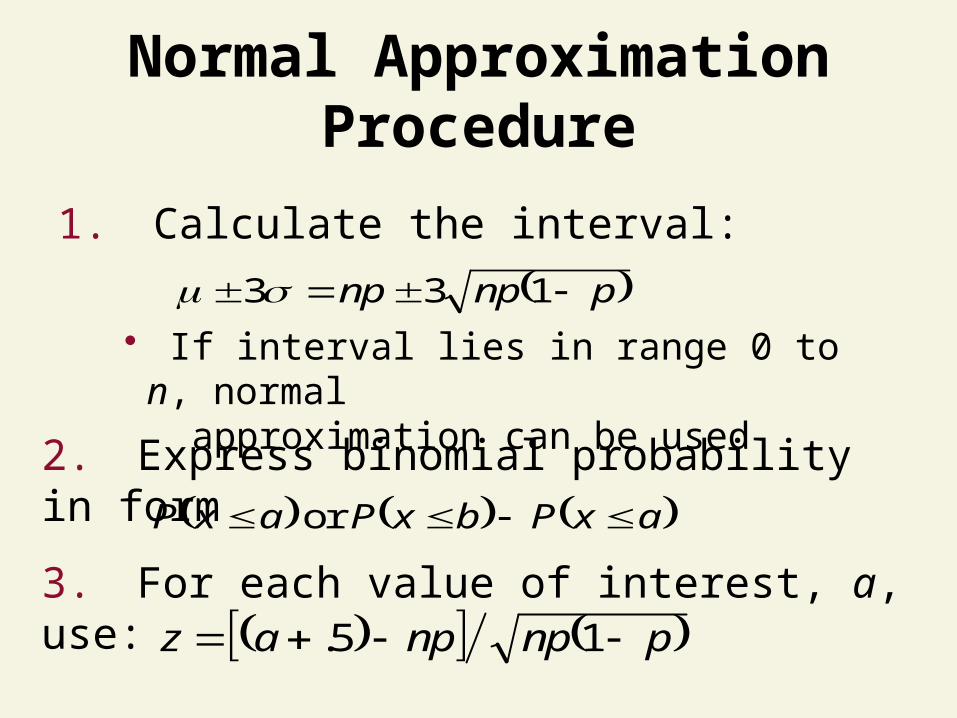
Normal Approximation Procedure
axPbxPaxP or
2. Express binomial probability in form
pnpnpaz 15.
3. For each value of interest, a, use:
133 pnpnp
1. Calculate the interval:
• If interval lies in range 0 to n, normal approximation can be used
.0
.1
.2
.3
0 2 4 6 8 10
x
P(x)
Normal Approximation Example
3.5 4.5
What is the normal approximation of p(x = 4) given n = 10, and p = 0.5?
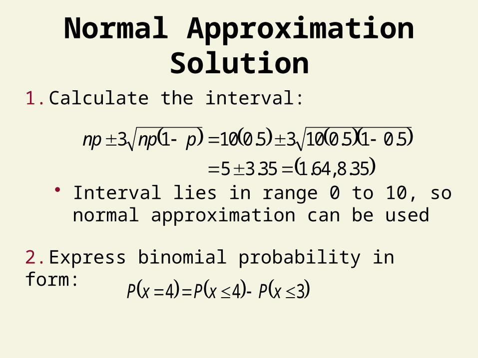
Normal Approximation Solution
1. Calculate the interval:
• Interval lies in range 0 to 10, so normal approximation can be used
35.8 ,64.135.35
5.015.01035.01013
pnpnp
2. Express binomial probability in form:
344 xPxPxP
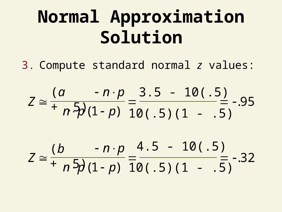
Normal Approximation Solution
Z(a + .5) n p
n p p
( )
.1
3.5 - 10(.5)
10(.5)(1 - .5)95
Zn p
n p p
( )
.1
4.5 - 10(.5)
10(.5)(1 - .5)32
(b + .5)
3. Compute standard normal z values:
= 0 = 1
-.32 Z-.95
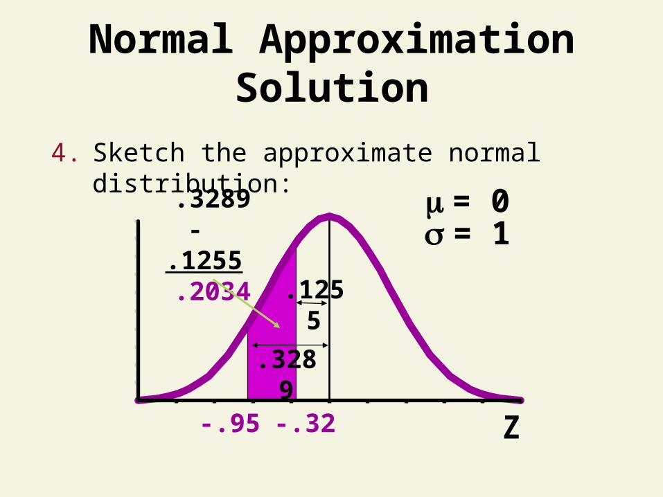
Normal Approximation Solution
.1255
.3289- .1255
.2034
.3289
4. Sketch the approximate normal distribution:
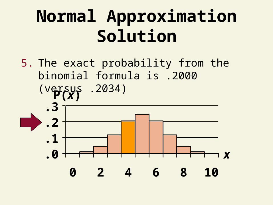
Normal Approximation Solution
.0
.1
.2
.3
0 2 4 6 8 10
x
P(x)
5. The exact probability from the binomial formula is .2000 (versus .2034)
91
Sampling Distributions

Parameter & Statistic
Parameter• Summary measure about
population
Sample Statistic• Summary measure about
sample
• P in Population & Parameter
• S in Sample & Statistic
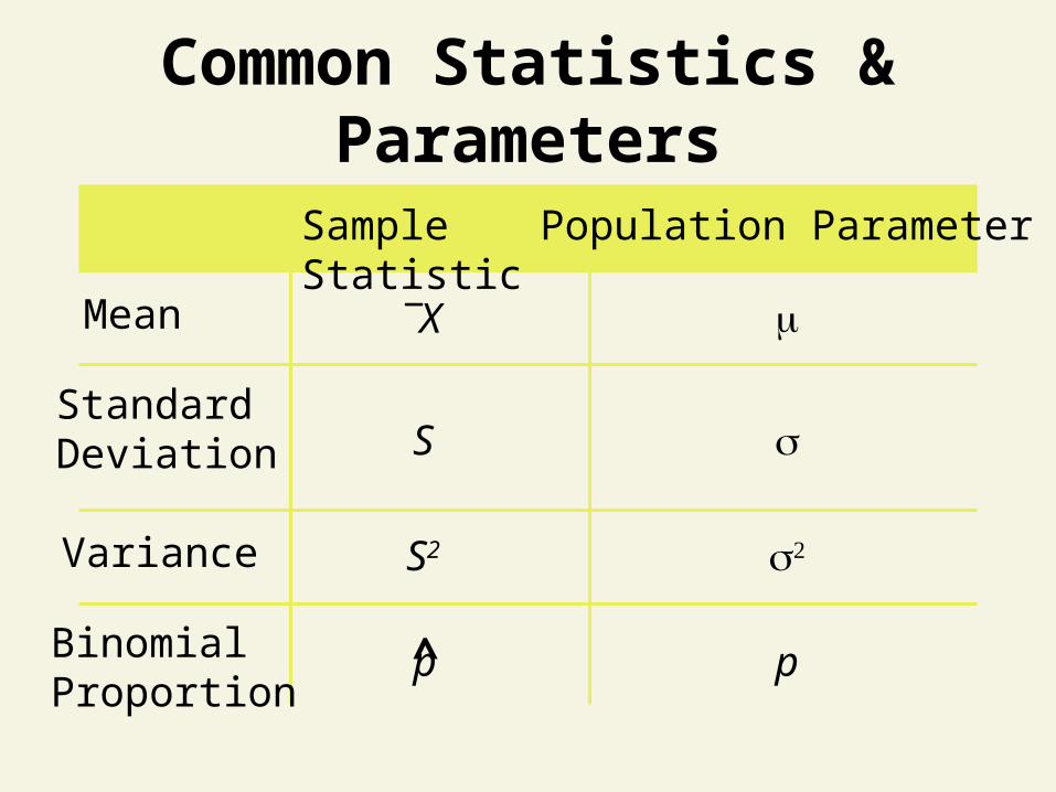
Common Statistics & Parameters
Sample Statistic Population Parameter
Variance S2 2
StandardDeviation S
Mean X
Binomial Proportion
pp̂
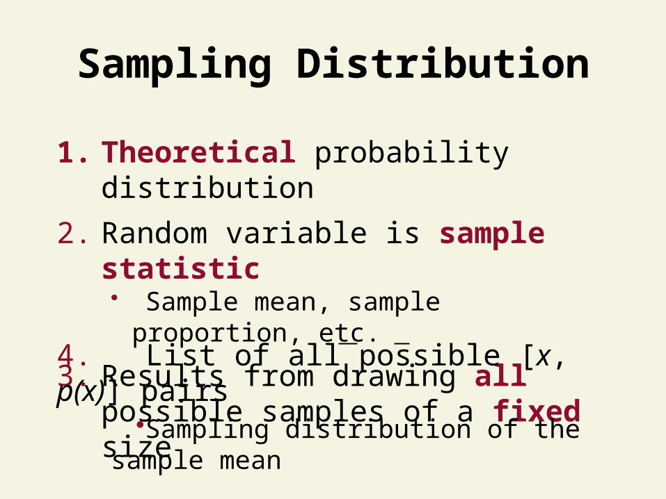
1. Theoretical probability distribution
2. Random variable is sample statistic• Sample mean, sample proportion, etc.
3. Results from drawing all possible samples of a fixed size
Sampling Distribution
4. List of all possible [x, p(x)] pairs•Sampling distribution of the sample mean
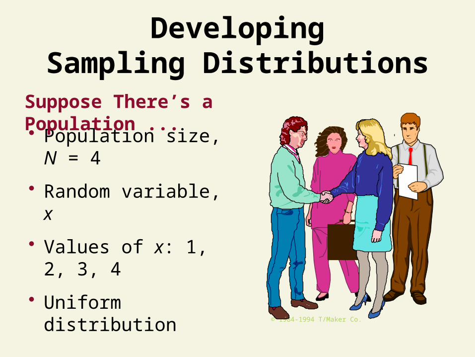
DevelopingSampling Distributions
• Population size, N = 4
• Random variable, x
• Values of x: 1, 2, 3, 4
• Uniform distribution
© 1984-1994 T/Maker Co.
Suppose There’s a Population ...
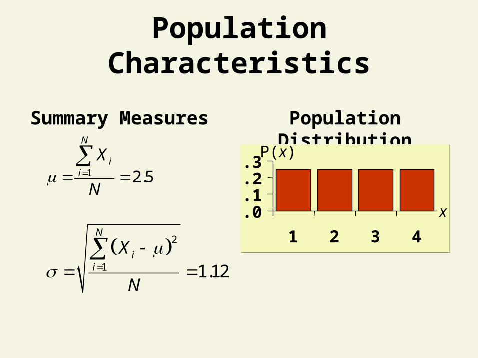
Population Characteristics
1 2.5
N
ii
X
N
Population DistributionSummary Measures
.0
.1
.2
.3
1 2 3 4 2
1 1.12
N
ii
X
N
P(x)
x
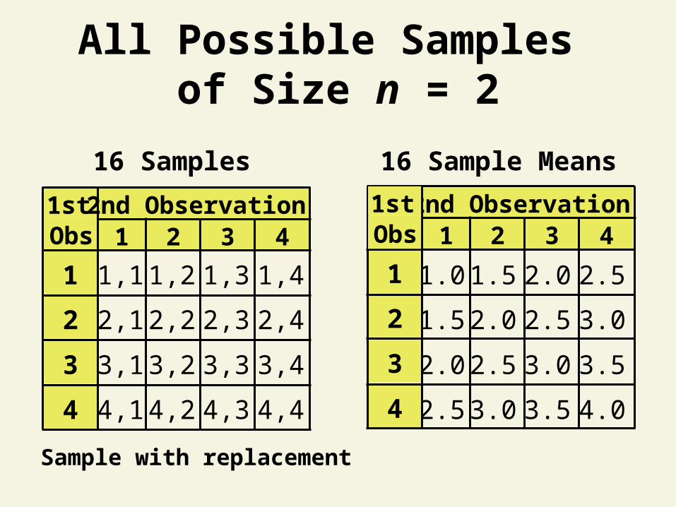
All Possible Samples of Size n = 2
Sample with replacement
1.0 1.5 2.0 2.5
1.5 2.0 2.5 3.0
2.0 2.5 3.0 3.5
2.5 3.0 3.5 4.0
16 Samples
1stObs
1,1 1,2 1,3 1,4
2,1 2,2 2,3 2,4
3,1 3,2 3,3 3,4
4,1 4,2 4,3 4,4
2nd Observation1 2 3 4
1
2
3
4
2nd Observation1 2 3 4
1
2
3
4
1stObs
16 Sample Means
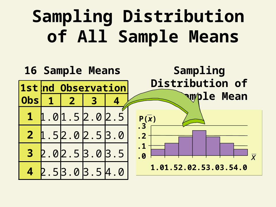
Sampling Distribution of All Sample Means
1.0 1.5 2.0 2.5
1.5 2.0 2.5 3.0
2.0 2.5 3.0 3.5
2.5 3.0 3.5 4.0
2nd Observation1 2 3 4
1
2
3
4
1stObs
16 Sample Means Sampling Distribution of the Sample Mean
.0
.1
.2
.3
1.0 1.5 2.0 2.5 3.0 3.5 4.0
P(x)
x
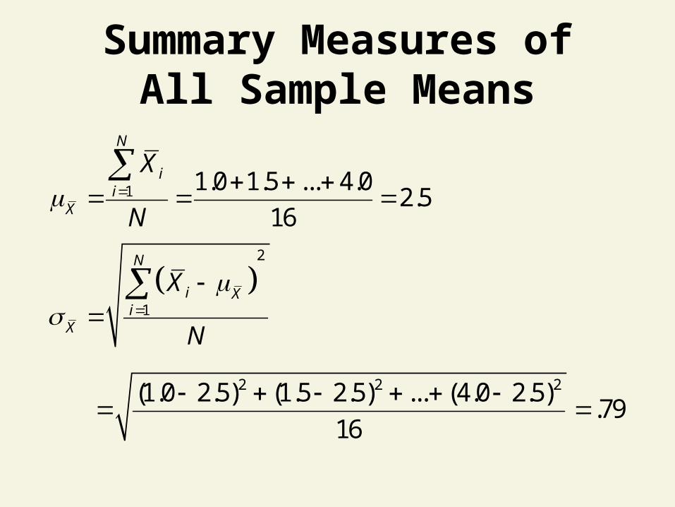
Summary Measures ofAll Sample Means
1 1.0 1.5 ... 4.02.5
16
N
ii
X
X
N
2
1
N
i Xi
X
X
N
2 2 2(1.0 2.5) (1.5 2.5) ... (4.0 2.5).79
16
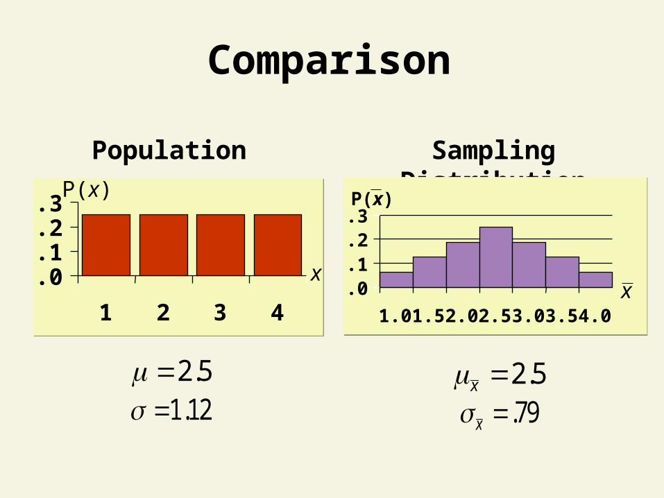
Comparison
Population Sampling Distribution
2.5x .79x
.0
.1
.2
.3
1 2 3 4
2.5 1.12
.0
.1
.2
.3
1.0 1.5 2.0 2.5 3.0 3.5 4.0
P(x)
x
P(x)
x

Standard Error of the Mean
xn
3. Formula (sampling with replacement)
2. Less than population standard deviation
1. Standard deviation of all possible sample means, x
● Measures scatter in all sample means, x
Properties of the Sampling Distribution of x
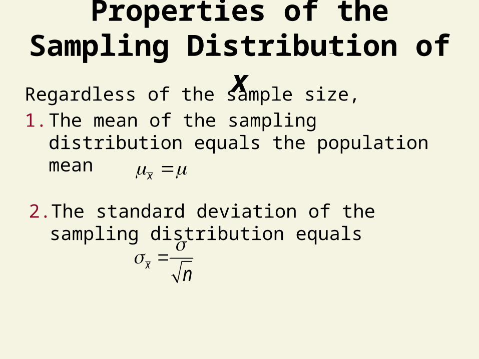
Properties of the Sampling Distribution of x
xn
2. The standard deviation of the sampling distribution equals
Regardless of the sample size,
1. The mean of the sampling distribution equals the population mean
x
Sampling from Normal Populations
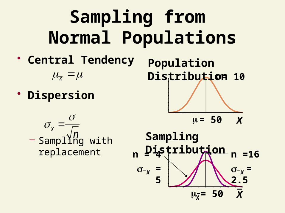
Sampling from Normal Populations
• Central Tendency
• Dispersion
– Sampling with replacement
m = 50
s = 10
X
n =16
X = 2.5
n = 4
X = 5
mX = 50- X
Sampling Distribution
Population Distributionx
xn
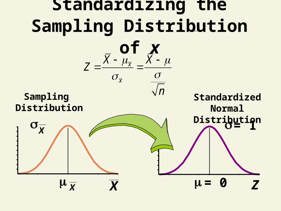
Standardizing the Sampling Distribution of x
Standardized Normal Distribution
m = 0
s = 1
Z
x
x
X XZ
n
Sampling Distribution
XmX
sX
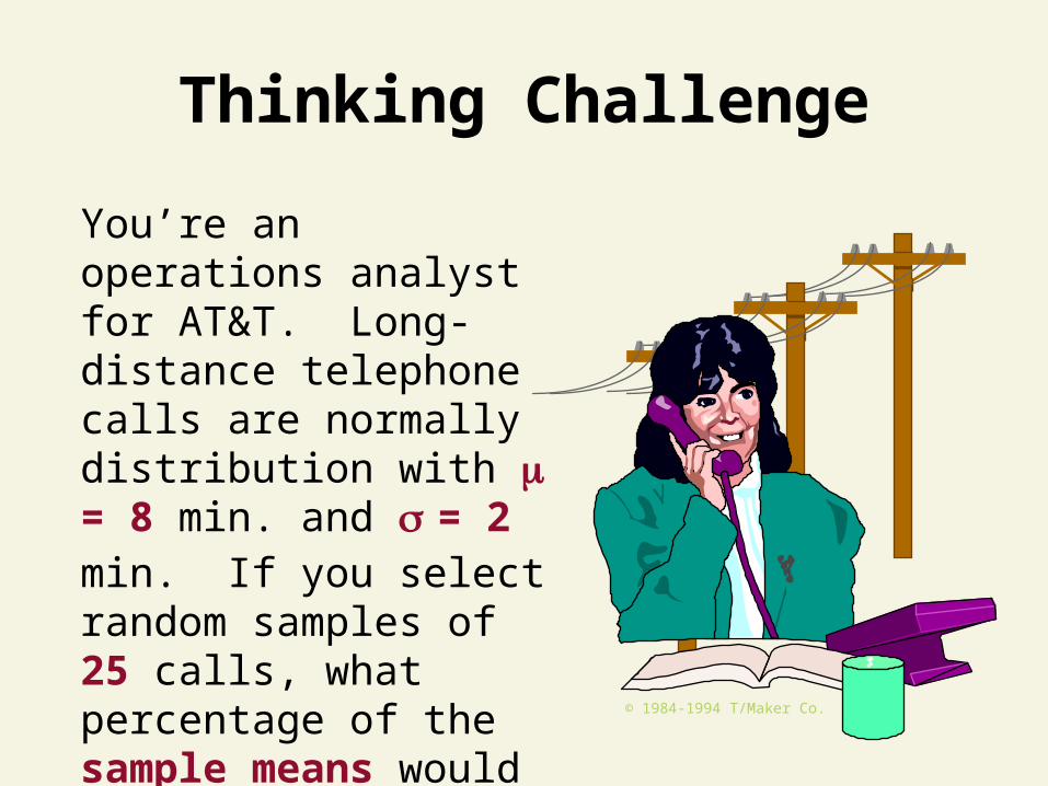
Thinking Challenge
You’re an operations analyst for AT&T. Long-distance telephone calls are normally distribution with = 8 min. and = 2 min. If you select random samples of 25 calls, what percentage of the sample means would be between 7.8 & 8.2 minutes?
© 1984-1994 T/Maker Co.
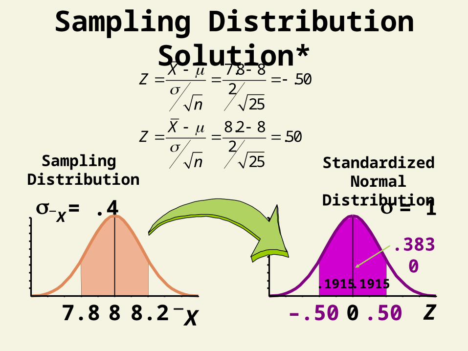
Sampling Distribution Solution*
Sampling Distribution
8
s `X = .4
7.8 8.2 `X 0
s = 1
–.50 Z.50
.3830
Standardized Normal Distribution
.1915.1915
7.8 8.50
225
8.2 8.50
225
XZ
n
XZ
n
Sampling from Non-Normal Populations
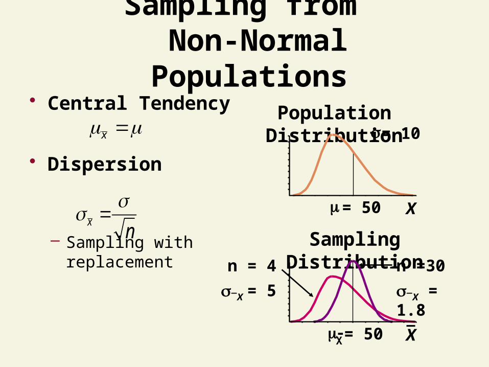
Sampling from Non-Normal Populations
• Central Tendency
• Dispersion
– Sampling with replacement
Population Distribution
Sampling Distributionn =30
X = 1.8
n = 4
X = 5
m = 50
s = 10
X
mX = 50- X
x
xn

Central Limit Theorem
X
As sample size gets large enough (n 30) ...
sampling distribution becomes almost normal.
x
xn
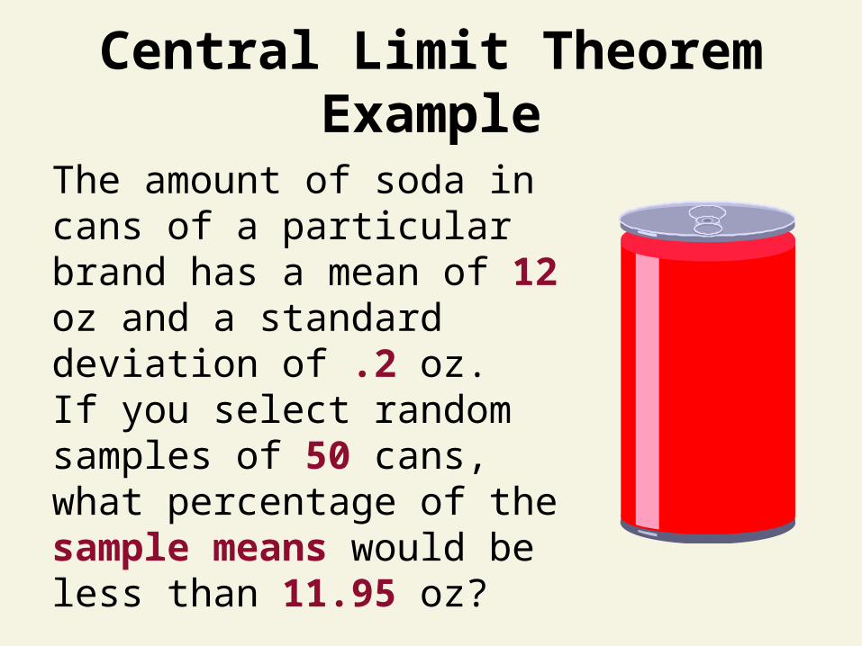
Central Limit Theorem Example
SODA
The amount of soda in cans of a particular brand has a mean of 12 oz and a standard deviation of .2 oz. If you select random samples of 50 cans, what percentage of the sample means would be less than 11.95 oz?
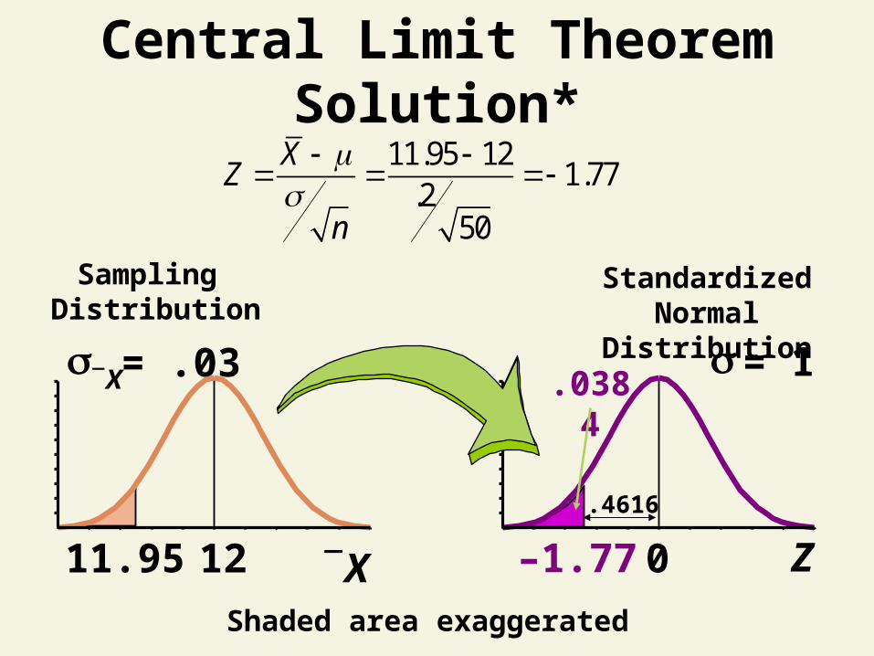
Central Limit Theorem Solution*
Sampling Distribution
12
s `X = .03
11.95 `X 0
s = 1
–1.77 Z
.0384
Standardized Normal Distribution
.4616
11.95 121.77
.250
XZ
n
Shaded area exaggerated
Conclusion
1. Distinguished Between the Two Types of Random Variables
2. Described Discrete Probability Distributions
3. Described the Binomial and Poisson Distributions
4. Described the Uniform and Normal Distributions
5. Approximated the Binomial Distribution Using the Normal Distribution
Conclusion (continued)
6. Explained Sampling Distributions
7. Solved Probability Problems Involving Sampling Distributions
Recommended