Stochastic Inventory Theory
Professor Stephen R. LawrenceLeeds School of BusinessUniversity of ColoradoBoulder, CO 80309-0419

Stochastic Inventory Theory
Single Period Stochastic Inventory Model “Newsvendor” model
Multi-Period Stochastic Inventory Models Safety Stock Calculations Expected Demand & Std Dev Calculations Continuous Review (CR) models Periodic Review (PR) models
Single Period Stochastic Inventory
“Newsvendor” Model

Single-Period Independent Demand “Newsvendor Model:” One-time buys of
seasonal goods, style goods, or perishable items
Examples: Newspapers, Christmas trees; Supermarket produce; Fad toys, novelties; Fashion garments; Blood bank stocks.

Newsvendor Assumptions
Relatively short selling season; Well defined beginning and end; Commit to purchase before season starts; Distribution of demand known or estimated; Significant lost sales costs (e.g. profit); Significant excess inventory costs.

Single-Period Inventory Example
A T-shirt silk-screening firm is planning to produce a number of custom T-shirts for the next Bolder Boulder running event. The cost of producing a T-shirt is $6.00, with a selling price of $12.00. After BB concludes, demand for T-shirts falls off, and the manufacturer can only sell remaining shirts for $3.00 each. Based on historical data, the expected demand distribution for BB T-shirts is:
How many T-shirts should the firm produce to maximize profits?
Quantity Probability Cumulative
1000 0.00 0.00
2000 0.05 0.05
3000 0.15 0.20
4000 0.40 0.60
5000 0.30 0.90
6000 0.10 1.00

Opportunity Cost of Unmet Demand
Define:
U = opportunity cost of unmet demand (underproduce - understock)
Example:
U = sales price - cost of production
= 12 - 6
= $6 lost profit / unit

Cost of Excess Inventory
Define:
O = cost of excess inventory
(overproduce - overstock)
Example:
O = cost of production - salvage price
= 6 - 3
= $3 loss/unit

Solving Single-Period Problems
Where Pr(x≤Q*) is the “critical fractile” of the demand distribution.
ExampleU = cost of unmet demand (understock) U = 12 - 6 = 6 profitO = cost of excess inventory (overstock) O = 6 - 3 = 3 loss
Produce/purchase quantity Q* that satisfies the ratio
Optimal Solution:
OU
UQx
)Pr( *

Translation to Textbook Notation
Lawrence Textbook
Understock cost U Cus
Overstock cost O Cos
Probability of understocking
Pr(xQ) Pus
Critical fractile Pr(xQ)Critical fillrate (cfr)

Alternate Solution
Where Pr(x>Q*) is the “critical fractile” that represents the probability of a stockout when starting with an inventory of Q* units.
Produce/purchase quantity Q* that satisfies the ratio
OU
O
OU
UQxQx
1)Pr(1)Pr( **
Some textbooks use an alternative representation of the critical fractile:
NOTE: to use a standard normal Z-table, you will need Pr(x≤Q*), NOT Pr(x>Q*)

Solving Single-Period Problems
ExampleU = cost of unmet demand (underage) U = 12 - 6 = 6 profitO = cost of excess inventory (overage) O = 6 - 3 = 3 loss
Example:
Pr(x ≤ Q) = 6 / ( 3 + 6 ) = 0.667

Solving Single-Period Problems
D
0.00
0.20
0.40
0.60
0.80
1.00
1000 2000 3000 4000 5000 6000
Quantity (Q)
Pro
bab
ility
P(x
<Q)
0.667
4,222

Inventory Spreadsheet
Multi-Period Stochastic Inventory Models Continuous Review (CR) models
Periodic Review (PR) models

Key Assumptions
Demand is probabilistic Average demand changes slowly Forecast errors are normally distributed with
no bias Lead times are deterministic
Key Questions
How often should inventory status be determined?
When should a replenishment order be placed?
How large should the replenishment be?

Types of Multi-Period Models
(CR) continuous review Reorder when inventory falls to R (fixed) Order quantity Q (fixed) Interval between orders is variable
(PR) periodic review Order periodically every T periods (fixed) Order quantity q (variable) Inventory position I at time of reorder is variable
Many others…

Notation B = stockout cost per item TAC = total annual cost of inv. L = order leadtime D = annual demand d(L) = demand during leadtime h = holding cost percentage H = holding cost per item I = current inventory position
Q = order quantity (fixed) Q* = optimal order quantity q = order quantity (variable) T = time between orders R = reorder point (ROP) S = setup or order cost SS = safety stock C = per item cost or value.

Demand Calculations

Demand over Leadtime
Multiply known demand rate D by leadtime L Be sure that both are in the same units!
Example Mean demand is D = 20 per day Leadtime is L= 40 days d(L) = D x L = 20 x 40 = 800 units

Demand Std Deviation over Leadtime Multiply demand variance 2 by leadtime L Example
Standard deviation of demand = 4 units per day Calculate variance of demand 2 = 16 Variance of demand over leadtime L=40 days is
L2 = L 2 = 40×16=640
Standard deviation of demand over leadtime L is L = [L 2]½ = 640½ = 25.3 units
Remember Variances add, standard deviations don’t!

Safety Stock Calculations

Safety Stock Analysis
The world is uncertain, not deterministic demand rates and levels have a random component delivery times from vendors/production can vary quality problems can affect delivery quantities Murphy lives
safety stock
RL
time
Inventory Level
Q
0stockout!
SS

Inventory / Stockout Trade-offs
InventoryLevel
R
SS
0time
R
SS
SS
R
Large safety stocks Few stockouts
High inventory costs
Small safety stocks Frequent stockoutsLow inventory costs
Balanced safety stock, stockout frequency,
inventory costs

Safety Stock Example Service policies are often set by management
judgment (e.g., 95% or 99% service level) Monthly demand is 100 units with a standard deviation
of 25 units. If inventory is replenished every month, how much safety stock is need to provide a 95% service level? Assume that demand is normally distributed.
4225.412565.195.0 LzSS
Alternatively, optimal service level can be calculated using “Newsvendor” analysis

Continuous Review (CR) Stochastic Inventory Models

Always order the same quantity Q Replenish inventory whenever inventory level falls below
reorder quantity R Time between orders varies Replenish level R depends on order lead-time L Requires continuous review of inventory levels
RQ Q
Q
Q
L
time
Inventory Level
(CR) Continuous Review System
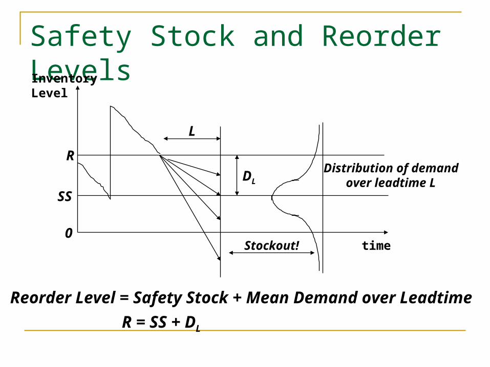
Safety Stock and Reorder Levels
Reorder Level = Safety Stock + Mean Demand over Leadtime
R = SS + DL
L
Distribution of demand over leadtime L
Stockout!
InventoryLevel
time
R
SS
0
DL

(CR) Order-Point, Order-Quantity
Continuous review system Useful for class A, B, and C inventories Replenish when inventory falls to R; Reorder quantity Q. Easy to understand, implement “Two-bin” variation

(CR) Implementation
Implementation Determine Q using EOQ-type model Determine R using appropriate safety-stock model
Practice Reserve quantity R in second “bin” (i.e. a baggy) Put order card with second bin Submit card to purchasing when second bin is
opened Restock second bin to R upon order arrival

(CR) Example
Consider a the following product D = 2,400 units per year C = $100 cost per unit h = 0.24 holding fraction per year (H = hC = $24/yr) L = 1 month leadtime S = $ 200 cost per setup B = $ 500 cost for each backorder/stockout L = 125 units per month variation
Management desires to maintain a 95% in-stock service level.

(CR) Example
20012/400,2 LD
200)100)(24.0(
2400)(200(22* hC
SDQ
406206200)125(65.1200
200 95.0
R
zSSDR LL
Whenever inventory falls below 406, place another order for 200 units

Total Inventory Costs for CR Policies TAC = Total Annual Costs TAC = Ordering + Holding + Expected Stockout Costs
1004430073442400
)05.0(200
2400500
2
20020624
200
2400200
)Pr(2
TAC
TAC
QdQ
DB
QSSH
Q
DSTAC
TAC = $10,044 per year (CR policy)
Periodic Review (PR) Stochastic Inventory Models

Multi-Period Fixed-Interval Systems
Requires periodic review of inventory levels Replenish inventories every T time units Order quantity q (q varies with each order)
T TT
L L L
I
II
Inve
nto
ry L
evel
time
q
q
q

Periodic Review Details Order quantity q must be large enough to cover
expected demand over lead time L plus reorder period T (less current inventory position I )
Exposed to demand variation over T+L periods
T TT
L L L
I
II
Inve
nto
ry L
evel
time
q
q
q

(PR) Periodic-Review System
Periodic review (often Class B,C inventories) Review inventory level every T time units Determine current inventory level I Order variable quantity q every T periods Allows coordinated replenishment of items Higher inventory levels than continuous
review policies

(PR) Implementation
Implementation Determine Q using EOQ-type model; Set T=Q/D (if possible --T often not in our control) Calculate q as sum of required safety stock,
demand over leadtime and reorder interval, less current inventory level
Practice Interval T is often set by outside constraints E.g., truck delivery schedules, inventory cycles, …

(PR) Policy Example Consider a product with the following
parameters: D = 2,400 units per year C = $100 h = 0.24 per year (H = hC = $24/yr) T = 2 months between replenishments L = 1 month S = $200 B = $500 cost for each backorders/stockouts I = 100 units currently in inventory L= 125 units per month variation
Management desires to maintain a 95% in-stock service level.

(PR) Policy ExamplemonthsT 2
900857100357600
100)51.216(65.1600
)()( 95.0
q
q
IzLTdISSLTdq LT
mosmomosLT 312
600200400)()()( LdTdLTd
unitsLT 51.216)125(3 2
Suppose that this is given by circumstances…

Total Inventory Costs for PR Policies TAC = Total Annual Costs TAC = Ordering + Holding + Expected Stockout Costs
14718150133681200
)05.0)(6(5002
40035724)6(200
)Pr(2
TAC
TAC
QdQ
DB
QSSH
Q
DSTAC
TAC = $14,718 per year (PR policy)

Further Information
American Production and Inventory Control Society (APICS) www.APICS.org
Professional organization of production, inventory, and resource managers
Offers professional certifications in production, inventory, and resource management

Further Information
Institute for Supply Management (www.ISM.ws) Previously the National Association of Purchasing
Managers (NAPM) Professional organization of supply chain
managers Offers certifications in supply chain
management
Recommended